Embed Size (px)
Citation preview
LOAD RESISTANCE FACTOR DESIGN (LRFD) FOR DRIVEN PILES BASED ONDYNAMIC METHODS WITH ASSESSMENT OF SKIN AND TIP RESISTANCE
FROM PDA SIGNALS
By
ARIEL PEREZ PEREZ
A THESIS PRESENTED TO THE GRADUATE SCHOOLOF THE UNIVERSITY OF FLORIDA IN PARTIAL FULFILLMENT
OF THE REQUIREMENTS FOR THE DEGREE OFMASTER OF ENGINEERING
UNIVERSITY OF FLORIDA
1998

Copyright 1998
by
Ariel Perez

To my parents

iv
ACKNOWLEDGMENTS
Above all, I would like to thank all the geotechnical engineering staff. With their
knowledge, teaching skills, experience, and professionalism, they have provided me with
an excellent level of education. I wish to express my sincere appreciation and gratitude to
the chairman of my supervisory committee, Dr. Michael C. McVay, for providing me
with the opportunity to conduct this research and for his generous assistance and guidance
throughout the course of this study. Grateful acknowledgment is also made to Dr. Frank
C. Townsend for serving as committee member and sharing with me his extensive
experience in the geotechnical field. Special thanks are given to Dr. Fernando E.
Fagundo. Besides being a committee member, Dr. Fagundo has offered me his support
and friendship from our first meeting before arriving to Gainesville. Lastly, I would like
to acknowledge Dr. Limin Zhang, for his continuing guidance and encouragement in the
preparation of this manuscript. Without his work, this project would not have been
accomplished.
I wish to thank all my friends here in Gainesville, especially Alvin Gutierrez,
Beatriz Camacho, Elzys Boscan, Nereida Padrón and Gabriel Alcaraz. Their friendship
has provided me with life experiences I could not have gained elsewhere.
I am deeply grateful to Paul Bullock and Tanel Esin from Schmertmann &
Crapps, Inc. for their assistance in providing useful load test data appearing in this thesis.
The help from Dr. Ching L. Kuo from PSI, Inc. is also gratefully appreciated. Dr. Ching

v
Kuo was always willing to help by providing any requested information or by sharing his
vast experience in the deep foundation field. The funding of this research by the Florida
Department of Transportation is also acknowledged and appreciated.

vi
TABLE OF CONTENTS
page
ACKNOWLEDGMENTS.................................................................................................. iv
ABSTRACT....................................................................................................................... ix
CHAPTERS
1 INTRODUCTION......................................................................................................... 1
2 REVIEW OF FLORIDA PILE DRIVING PRACTICE................................................ 4Current Florida Practice................................................................................................ 4
Bearing Requirements............................................................................................. 4Blow count criteria............................................................................................ 5Practical refusal ................................................................................................. 5Set-checks and pile redrive................................................................................ 5Pile heave.......................................................................................................... 6Piles with insufficient bearing........................................................................... 6
Methods to Determine Pile Capacity....................................................................... 6Wave equation................................................................................................... 7Bearing formulas............................................................................................... 9Dynamic load tests............................................................................................ 9Static load tests.................................................................................................. 9
Evaluation of Florida Practice Changes...................................................................... 10Bearing Requirements........................................................................................... 10Methods to Determine Pile Capacity..................................................................... 11
3 PILE CAPACITY ASSESSMENT USING STATIC AND DYNAMICMETHODS.................................................................................................................. 14Davisson’s Capacity.................................................................................................... 14Dynamic Methods Review .......................................................................................... 16
Momentum Conservation...................................................................................... 16ENR................................................................................................................. 16Modified Engineering News Record formula................................................. 17FDOT .............................................................................................................. 18Gates method................................................................................................... 19
Combined Wave Mechanics and Energy Conservation........................................ 19Sakai et al. Japanese energy method ............................................................... 19Paikowsky’s method........................................................................................ 20
Wave Mechanics................................................................................................... 21
vii
PDA method.................................................................................................... 21CAPWAP program.......................................................................................... 25
4 UNIVERSITY OF FLORIDA PILE DATABASE..................................................... 27General Information and History................................................................................. 27PILEUF Information ................................................................................................... 29
General .................................................................................................................. 29Soil Classification ................................................................................................. 29Driving Information .............................................................................................. 30Dynamic Data (CAPWAP and PDA).................................................................... 31Load Test Results.................................................................................................. 31SPT94 Capacity..................................................................................................... 32
Gathering New Information ........................................................................................ 32Additional Required Information.......................................................................... 33Criteria for New Entries........................................................................................ 33
5 ASD AND LRFD CONCEPTS................................................................................... 34Allowable Stress Design (ASD) Method .................................................................... 34Load Resistance Factor Design (LRFD) Method........................................................ 35
Advantages of LRFD Over ASD........................................................................... 36Limitation of LRFD............................................................................................... 36
Calibration of LRFD ................................................................................................... 37Engineering Judgement ......................................................................................... 37Fitting ASD to LRFD............................................................................................ 37Reliability Calibration........................................................................................... 39
Statistical data................................................................................................. 39Probability density function ............................................................................ 41LRFD components.......................................................................................... 42
6 LRFD DATA PRESENTATION AND ANALYSIS.................................................. 51Data Reduction............................................................................................................ 51LRFD Analysis of Results........................................................................................... 56
Effect of Bridge Span Length and Probability of Failure...................................... 57Level of Conservatism and Accuracy Indicators................................................... 60φ/λR Ratio.............................................................................................................. 63
Methods comparison....................................................................................... 64EOD versus BOR............................................................................................ 64Evaluation of cases with capacity smaller or larger than 1779 kN ................. 64
Recommended Safety Factors............................................................................... 65ASD Design Evaluation ........................................................................................ 68
7 SKIN AND TIP STATIC CAPACITY ASSESSMENT OF DRIVEN PILES........... 69Method 1 ..................................................................................................................... 70Method 2 (Suggested) ................................................................................................. 72
Description and Main Assumptions...................................................................... 72Case Damping Coefficient, Jc , versus Tip to Skin Ratio....................................... 75Sensitivity Analysis of Case Damping Coefficient, Jc .......................................... 77
viii
Static and Dynamic Load Test Data...................................................................... 78Automating the Suggested Method....................................................................... 79
Results and Analysis ................................................................................................... 81Presentation of Results.......................................................................................... 81Analysis of Total Capacity Predictions................................................................. 86Analysis of Skin and Tip Capacity Predictions..................................................... 87Sensitivity of Jc and Pile Resistance...................................................................... 91
8 CONCLUSIONS AND RECOMMENDATIONS...................................................... 94LRFD Calibration for Eight Dynamic Methods.......................................................... 94
Conclusions........................................................................................................... 94Recommendations................................................................................................. 95
Suggested Method to Determine Pile Capacity........................................................... 96Conclusions........................................................................................................... 96Recommendations................................................................................................. 98
APPENDICES
A LRFD ANALYSIS RESULTS - CAPWAP PROCEDURE....................................... 99
B LRFD ANALYSIS RESULTS – PDA METHOD.................................................... 104
C LRFD ANALYSIS RESULTS – PAIKOWSKY’S ENERGY METHOD............... 109
D LRFD ANALYSIS RESULTS – SAKAI ET AL (JAPANESE) METHOD ............ 114
E LRFD ANALYSIS RESULTS – FDOT METHOD ................................................. 119
F LRFD ANALYSIS RESULTS – ENGINEERING NEWS RECORD (ENR).......... 128
G LRFD ANALYSIS RESULTS – MODIFIED ENR.................................................. 137
H LRFD ANALYSIS RESULTS – GATES FORMULA............................................. 146
I FORCE AND VELOCITY TRACES FROM PDA SIGNAL .................................. 155
J OUTPUT FILE FOR SUGGESTED METHOD & GRL PROCEDURE(FORTRAN).............................................................................................................. 179
LIST OF REFERENCES................................................................................................ 185
BIOGRAPHICAL SKETCH........................................................................................... 187
ix
Abstract of Thesis Presented to the Graduate Schoolof the University of Florida in Partial Fulfillment of theRequirements for the Degree of Master of Engineering
LOAD RESISTANCE FACTOR DESIGN (LRFD) FOR DRIVEN PILES BASED ONDYNAMIC METHODS WITH ASSESSMENT OF SKIN AND TIP RESISTANCE
FROM PDA SIGNALS
By
Ariel Perez Perez
December, 1998
Chairman: Dr. Michael C. McVayMajor Department: Civil Engineering
Eight dynamic methods to estimate the static capacity of driven piles were
evaluated based on a Florida database and Load Resistance Factor Design (LRFD). The
dynamic methods investigated were four stress wave approaches (CAPWAP, PDA,
Paikowsky Energy, and Sakai Energy) and four driving formulas (ENR, modified ENR,
FDOT, and Gates). In the case of the older driving formulas, the database was broken
into both small (i.e. Davisson capacity less than 1779 kN) and large (Davisson capacity
larger than 1779 kN) capacity piles. It was demonstrated that the modern methods based
on wave mechanics, such as CAPWAP, PDA, and Paikowsky’s energy method, are more
accurate than the old driving formulas. The utilizable measured Davisson capacity,
defined as φ/λR (ratio of resistance / mean capacity), shows that the new dynamic
methods are more cost effective to meet a reliability index in comparison with the old
x
methods based on momentum conservation. In addition, the Gates formula, when used
separately for Davisson capacity larger than 1779 kN or less than 1779 kN, may have
comparable accuracy with the modern methods.
A suggested empirical method is presented to calculate the total, skin, and tip
static resistance of driven piles. This method has proved to be equally or more accurate
than the most widely used method (i.e. PDA, and CAPWAP). Additional features of the
suggested method include determining the total, skin, and tip static capacities as the piles
are being driven, saving construction time, therefore, saving construction costs.
1
CHAPTER 1
INTRODUCTION
Dynamic testing has been a tool for estimating pile capacities and hammer
suitability since 1888 when the first driving formula, i.e. the Engineering News formula,
was published. From then to the early seventies, many driving formulas were proposed
and adopted into codes, all derived on the principles of impulse-momentum conservation.
In the sixties, pioneer research investigated predicting both stresses and pile capacities
based on wave mechanics. The results were the creation of programs such as, WEAP
(GRL, 1993), PDA (Pile Dynamics Inc., 1992), and CAPWAP (GRL, 1996). Recently,
energy approaches based on both wave mechanics and energy conservation have been
developed to determine the pile capacity.
Since the implementation of the PDA and CAPWAP about fifteen years ago, it is
unknown the accuracy of these methods in comparison with the older driving formulas.
Moreover, it is unknown how the newer energy equations compare to the past and present
methods for Florida soil conditions.
Recently, the American Association of State Highway and Transportation
Officials (AASHTO) has moved from the Allowable Stress Design (ASD) to the Load
Resistance Factor Design (LRFD) analysis. The latter method employs resistance factor,
φ, based on reliability indexes. However, in order to determine the accurate resistance
2
factors, the LRFD requires a database to assess the probability of failure of a given
method.
Based on the University of Florida pile database and AASHTO’s recommended
reliability index, and live to dead load ratios, the resistance factors (LRFD) and
equivalent safety factors (ASD) were developed for a number of dynamic pile capacity
methods. These parameters served as a tool to evaluate the accuracy and level of
prediction of the dynamic methods studied. The dynamic methods investigated were four
stress wave approaches (CAPWAP, PDA, Paikowsky Energy, and Sakai Energy) and four
driving formulas (ENR, modified ENR, FDOT, and Gates). In the case of the older
driving formulas, the database was broken into both small (i.e. Davisson capacity less
than 1779 kN) and large (Davisson capacity larger than 1779 kN) capacity piles.
Since 1994, the Florida Department of Transportation specifications recommend
the use of Wave Equations to determine the suitability of the driving system and to
estimate the pile capacity. It is also recommended the use of dynamic and/or static load
tests to verify the estimated capacity. For the dynamic procedures, FDOT recommends
the use of PDA or CAPWAP only. The capability of CAPWAP to estimate the skin and
tip capacity in addition to the distribution of damping through the pile have created a
level of confidence in the pile industry over the PDA whose result consists only of the
total static capacity. However, the CAPWAP program needs highly trained people to run
it, and involves a series of iterations. The latter creates delays in the pile driving
operations and increase in foundation costs.
A suggested empirical method is presented to calculate the total, skin, and tip
static resistance of driven piles using the PDA Case solution. This method has proved to

3
be equally or more accurate than the most widely used methods (i.e. PDA, CAPWAP). In
addition, the suggested method allows the users to determine the pile capacities instantly
as the piles are driven, saving construction time. Because all the calculations for the
suggested method are performed automatically, a technician with a high level of expertise
is not required.
4
CHAPTER 2
REVIEW OF FLORIDA PILE DRIVING PRACTICE
In this chapter, the pile driving practice in Florida will be presented. Because the
Florida Department of Transportation (FDOT) uses a large percentage of driven piles
versus the private industry, the information presented herein is based on their
recommendations. It is the author’s intention to present the current driving practice
together with a discussion of the most relevant changes throughout the years. This
discussion is focussed on aspects such as bearing requirements, and methods to determine
pile capacity.
Current Florida Practice
The information presented is in relation to the current Florida practice, which was
obtained from the FDOT Standard Specifications for Road and Bridge Construction of
1999. For more details, the reader is referred to the latest FDOT specifications.
Bearing Requirements
As a general criterion the engineer in charge of the driving process may accept a
driven pile if it has achieved the minimum penetration, the blow count has a tendency to
increase and the minimum bearing capacity is obtained for 600 mm of consecutive
driving. The engineer may also accept a driven pile if the minimum penetration was
reached and the driving has achieved practical refusal in firm strata. Aspects such as
5
practical refusal and others driving criteria will be discussed in detail in the following
sections.
Blow count criteria
Using the Wave Equation Analysis for Piles (WEAP) the engineer can determine
the number of blows per specific penetration to reach a design pile capacity. The blow
count has to be averaged for every 250 mm of pile penetration or through the last 10 to 20
blows of the hammer. It should be noted that the driving equipment must be selected in
order to provide the required resistance at a blow count ranging from 30 blows per 250
mm to 98 blows per 250 mm.
Practical refusal
Practical refusal is defined as a blow count of 20 blows per 25 mm for 50 mm of
driving. The FDOT specifications recommend that driving ceases after driving to
practical refusal conditions for 250 mm. If the required penetration can not be achieved
by driving without exceeding practical refusal, other alternates should be considered such
as jetting or Preformed Pile Holes.
Set-checks and pile redrive
Set-checks. Set checks are performed in the event that the Contractor has driven
the pile up to the point that the pile top elevation is within 250 mm of the cut-off
elevation and the pile has not reached the required resistance. Prior to a set check, the
driving process is interrupted for 15 minutes. Then, the engineer is provided with a level
or other suitable equipment to determine elevation in such a way that the pile penetration
during the set-checks could be determine in a very accurate manner. If the initial set-
6
check results are not satisfactory, additional set-checks could be performed. The pile is
then accepted if the pile has achieved the minimum required pile bearing.
Pile redrive. Pile redrive consists of redriving the pile after 72 hours from
original driving. The pile redrive is considered when time effect is important in the pile
capacity. Other considerations include the pile heave.
Pile heave
Pile heave is defined as the upward movement of a pile from its originally driven
elevation. In occasions, driving a pile can cause excessive heave and/or lateral
displacement of the ground. The previously driven pile should be monitored, and in the
event of pile heave (6 mm or more), all piles must be redriven unless the engineer has
determined that the heave is not detrimental to the pile capacity.
Piles with insufficient bearing
In the event that the pile top has reached the cut-off elevation without achieving
the required bearing resistance, the FDOT specifications recommends:
1. Splice the pile and continue driving.
2. Extract the pile and drive a pile of greater length.
3. Drive additional piles until reducing the adjusted required bearing per pile to
the bearing capacity of the piles already driven.
Methods to Determine Pile Capacity
The FDOT Specifications recommend the use of Wave Equation to determine pile
capacity for all structures or projects. The use of static load tests or dynamic load tests, or
both, is recommended to verify the capacity estimated from Wave Equation predictions.
7
Nevertheless, the prediction by the Wave Equation (blow count criteria) could be adjusted
to match the resistance determined from the static or dynamic load tests, or both.
Wave equation
The FDOT Specifications recommends to use the WEAP program to predict the
pile capacity. This program allows the engineer to evaluate other aspects of the driving
process. In the following paragraphs, a description of these aspects will be presented.
Evaluation of driving system. Evaluate the suitability of the driving system
(including hammer, follower, capblock and pile cushions. The driving system must be
capable of driving the pile to a resistance of 3.0 times the design load, plus the scour and
down drag resistance or the ultimate resistance, whichever is higher.
Determine pile driving resistance. The pile driving resistance, in blows per 250
mm or blows per 25 mm could be determined. The required driving resistance is defined
as the design load multiplied by the appropriate factor of safety plus the scour and down
drag resistance or the ultimate bearing capacity, whichever is higher.
Evaluate pile driving stresses. The engineer must evaluate the driving system to
avoid overstressing the pile at any moment during the driving. If the Wave Equation
analyses show that the hammer will overstress the pile, the driving system has to be
rejected. The FDOT Specifications 455-5.11.2 presents the allowable stresses for piles
made out of concrete, steel and timber. Equation 2-1, 2-2, and 2-3 give the maximum
allowable tensile and compression stresses for prestressed concrete piles.
The allowable compressive stress is,
pccapc ffs 75.07.0 1 −= (2-1)
8
For piles length less than 15 meters the allowable tensile stress is given by
( ) pccapt ffs 05.154.05.01 += (2-2)
And for piles length greater than 15 meters
( ) pccapt ffs 05.127.05.01 += (2-3)
where sapc Maximum Allowable Pile Compressive Stress, MPa
Sapt Maximum Allowable Pile Tensile Stress, MPa
fc1 Specified Minimum Compressive Strength of
Concrete, MPa.
fpc Effective Prestresses at Time of Driving.
For steel piles the maximum allowable compression and tensile stresses are equal
to ninety percent (90 %) of the yield strength (0.9 fy) of the steel. While for timber piles
the maximum allowable pile compression and tensile stresses are 25 MPa for Southern
Pine and Pacific Coast Douglas Fir and 0.9 of the ultimate parallel to the grain strength
for piles of other wood.
9
Bearing formulas
The FDOT under specification 455-5.11.3 recommends the following bearing
formula for temporary timber piles driven with power hammers:
54.2
167
+=
s
ER (2-4)
where R Safe Bearing Value, in Kilonewtons.
s The Average Penetration per Blow, in Millimeters.
E Energy per Blow of Hammer, in Kilojoules.
The latter specification also clearly states that this formula should not be used to
determine pile capacity of any other pile type. No other bearing formula is suggested in
the specifications for concrete or steel piles.
Dynamic load tests
Dynamic load testing consists of predicting pile capacity from blows of the
hammers during drive and/or redrive of an instrumented pile. Chapter 3 includes more
details of how the dynamic load test is performed (see PDA and CAPWAP sections).
Static load tests
Static load testing consists of applying a static load to the pile to determine its
capacity. The FDOT recommends the Modified Quick Test. For more details about the
static load test, the reader is referred to the FDOT specification 455-2.2.1. Some general

10
information about this test, and the procedure to obtain the pile capacity are explained in
Chapter 3.
Evaluation of Florida Practice Changes
In the following sections the most relevant changes in the Florida practice (i.e.
bearing requirements and proposed methods to determine pile capacity) for approximately
the last 10 years are discussed. For this purpose, the actual practice will serve as a
reference for any comparison. To facilitate the comparison process, only the changed
criteria will be discussed. The latter does not mean that the aspects not mentioned within
this document did not vary (i.e. only the topics related to this thesis will be investigated).
Because the largest change in FDOT specifications related to pile foundation were found
in the 1994 version versus 1991 version specifications, the discussion will be based on
these two references. To simplify the comparison, the FDOT specifications of 1991 and
prior to 1991 will be called “old specifications” and any other specification after 1991
will be called the “new specifications.”
Bearing Requirements
In general, there was a great change in the FDOT specifications of 1994 in
comparison to the older FDOT specifications. In the old specifications the piles were
allowed to be driven to grade. Even if the practical resistance had not been reached at
that point, the engineer was able to drive the pile below grade and build up. After driving
12 inches (0.305 m) below grade, a set-check could be performed after 12 hour of initial
driving. The latter criterion differs from the new practice in the elevation at which the

11
set-check is recommended. The new practice recommends the set-check to be performed
at approximately 10 inches above the cut-off elevation.
Another important difference is related to the bearing formulas. In the old
specifications, the FDOT recommend the use of bearing formulas to determine the pile
bearing capacity for piles made out of timber, concrete, composite concrete-steel and
steel. Then, from 1994 to date the specifications limited the use of bearing formulas to
timber piles driven with power hammers only.
Methods to Determine Pile Capacity
It was noted that in the old specifications there was not any requirement for using
Wave Equation programs to determine the pile capacity. The same observation applies to
the use of dynamic testing as a method to determine the pile capacity. Prior to 1994, the
FDOT recommended the use of static load test to determine the pile capacity of any pile
that did not reach the required resistance at the end of drive or as directed by the engineer.
The new specifications recommend the use of Pile Driving Analyzer (PDA), the Wave
Equation Analysis for Pile (WEAP), and the static load test separately or in a combination
of each, as recommended by the engineer (the safety factor for design depends upon the
number and kind of test performed).
The other difference is in the criterion for determining the pile capacity from the
static load test. In the old specifications, the failure criterion is given by either or both
conditions shown below:
1. One and one-half times the yield load settlement develops. The yield load is
defined as that load beyond which the total additional settlement exceeds 0.03
inch per ton, for the last increment applied.
12
2. The total permanent settlement of the top of the pile is greater than ¼ of an
inch.
The new specifications present two criteria to determine the static pile capacity.
Those criteria are as follows:
1. Davisson – for shafts with diameter up to 600 mm, the load that causes a shaft
top deflection equal to the calculated elastic compression, plus 4 mm, plus
1/120 of the shaft diameter in millimeters.
2. FHWA – for shafts with diameter larger than 600 mm, the load that causes a
shaft top deflection equal to the calculated elastic compression, plus 1/30 of the
shaft diameter.
The changes in criteria for selecting the failure load reflect, first, an increase in the
use of larger piles in the construction field, and second, the FDOT recognizes that for
larger piles (diameter larger than 600 mm) the capacity according to Davisson’s criterion
is conservative.
As a general observation, the FDOT has abandoned the old methods to determine
the bearing capacity of piles (i.e. bearing formulas, based on momentum conservation).
At the same time, the FDOT has adopted other prediction methods such as Wave
Equation, PDA, and CAPWAP, which are based on piles dynamic and wave propagation
through the pile, to estimate the static pile capacity. Other old methods such as Gates,
ENR, and Modified ENR are not considered as alternates in estimating the pile capacity,
neither are the relatively new methods such as Paikowsky’s method and Sakai et. al.
method.

13
It was proposed by the FDOT to investigate the new FDOT specifications in
relation to the old methods based on momentum conservation (i.e. FDOT, Gates, ENR,
Modified ENR). Another important consideration was to evaluate the old methods for
large capacity piles, which are used today, separately from small capacity piles (i.e. piles
with capacity up to 2000 kN approximately). The latter reflects the magnitude of design
loads for which piles were designed in the past in comparison to the present practice.
14
CHAPTER 3
PILE CAPACITY ASSESSMENT USING STATIC AND DYNAMIC METHODS
The Florida Department of Transportation (FDOT) under contract No. BB-349
required UF to evaluate the older empirical methods for determining pile capacity and
compare them to the modern instrumented methods. In addition, it was required to obtain
the resistance factor for each method (Load Resistance Factor Design - LRFD). In order
to perform the latter, the Davisson’s capacity served as the measured capacity for each
pile. In the following sections, a brief description of the Davisson criterion together with
the description of the empirical methods investigated will be presented.
Davisson’s Capacity
The Davisson method (Davisson, 1972) is one of many methods developed to
determine the pile capacity based on a static load test results. Davisson defined the pile
capacity as the load corresponding to the movement which exceeds the elastic
compression of the pile by a value of 4-mm (0.15 inches) plus a factor equal to the
diameter of the pile in millimeter divided by 120. Figure 3-1 presents the load-
displacement curve resulting from a static load test. From this curve, the Davisson’s pile
capacity can be obtained. The steps to obtain the Davisson’s capacity are as follow:
15
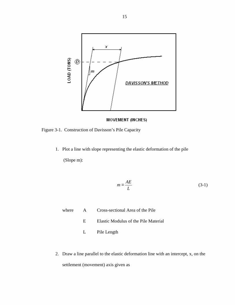
Figure 3-1. Construction of Davisson’s Pile Capacity
1. Plot a line with slope representing the elastic deformation of the pile
(Slope m):
L
AEm= (3-1)
where A Cross-sectional Area of the Pile
E Elastic Modulus of the Pile Material
L Pile Length
2. Draw a line parallel to the elastic deformation line with an intercept, x, on the
settlement (movement) axis given as
16
1200.4
Dx += (3-2)
where D Diameter of Pile in millimeters
x horizontal displacement of elastic deformation line
in millimeters
3. The Davisson’s capacity (point D on Figure 3-1) is defined as the intersection
point between the load-settlement curve and the elastic deformation line.
Dynamic Methods Review
Eight methods were considered in this study, which are subdivided in three
categories: momentum conservation, combined wave mechanics with energy
conservation, and wave mechanics alone. The methods are the Engineering News Record
(ENR), Modified ENR, FDOT, Gates, Paikowsky, Sakai (Japanese), Pile Driving
Analyzer (PDA) and the Case Pile Wave Analysis Program (CAPWAP). In the following
sections, a brief description of each method is presented.
Momentum Conservation
ENR
One of the older formulas developed to estimate the driven pile capacity was the
formula published in the Engineering News Record (ENR) (Coduto after Wellington,
1994). It has since become known as the Engineering News Record formula:
17
)1.0( +=
sF
hWP r
a (3-3)
where Pa Allowable Pile Load
Wr Hammer Ram Weight
h Hammer Stroke (the distance the hammer falls)
F Factor of Safety
s Pile Set (penetration) per Blow in Inches
Wellington (1888) recommended using a Safety Factor of 6.0.
Modified Engineering News Record formula
In 1961, the Michigan Highway Department (Housel, 1966) performed a series of
pile driving tests with the objective of evaluating the accuracy of the ENR formula. After
evaluating 88 piles, the investigators found that the ENR formula overpredicted the pile
capacities by a factor of 2 to 6. The findings mean that piles designed with a SF of 6 will
have a real factor of safety of 1 and 3. Based on their results, the Michigan Highway
Department developed the Modified Engineering News Formula:
))(1.0(
)(0025.0 2
Pr
Pra WWs
WeWEP
+++= (3-4)
where Pa Allowable Pile Load (kips)
18
E Rated Hammer Energy Per Blow (ft-lb)
WP Weight of Pile plus Driving Appurtenances (lb)
Wr Weight of Hammer Ram (lb)
s Pile Set (in/blow)
e Coefficient of Restitution
FDOT
The Florida Department of Transportation under specification 455-3.3 (1991)
recommends the following bearing formula (FDOT, 1991).
PS
ER
01.01.0
2
++= (3-5)
where R Safe Bearing Value in Tons
P Weight of Pile as Driven, in Tons
S Average Penetration per Blow, in Inches
E Energy per Blow of Hammer, in Foot-Tons
The last formula was used for concrete piles, composite concrete-steel piles and
steel piles. The bearing capacity obtained using the latter FDOT approach either
coincided or exceed the design capacity (suggested FS = 1.0).
19
Gates method
The method was the results of a research performed by Marvin Gates, J.M (1957).
The basic assumption is that the resistance is directly proportional to the squared root of
the net hammer energy. This relationship is presented by
( )sbEeaP hhu log−= (3-6)
where Pu Static Pile Resistance
eh Hammer Efficiency (0.85 used for all Cases)
Eh Hammer Energy
a, b 27 and 1.0 Respectively (English units)
s Point Permanent Penetration per Blow - Set
A suggested safety factor equal 3.0 is recommended.
Combined Wave Mechanics and Energy Conservation
Sakai et al. Japanese energy method
Sakai’s pile driving formula was developed based on stress-wave theory.
According to Sakai, this consideration introduced two advantages, it is theoretically
accurate as well as easy to use (Sakai et al., 1996). For a blow by an elastic hammer
Sakai et al. recommend
( )sDM
M
L
AER
H
P
Pu −
= max2
(3-7)
20
where A Pile Cross Sectional Area
E Young’s Modulus of Pile Material
LP Length of the Pile
MP Mass of the Pile
Dmax Maximum Penetration of Pile per Blow
s Permanent Set
Paikowsky’s method
The Paikowsky method or “Energy Approach” is a simplified energy approach
formulation for the prediction of pile resistance based on the dynamic measurements
recorded during driving. The basic assumption of the method is an elasto-plastic load
displacement pile-soil reaction. The Paikowsky method uses as input parameters the
maximum calculated transferred energy and maximum pile displacement from the
measured data together with the field blow count. Equation 3-8 presents the solution for
the dynamic pile capacity Ru (Paikowsky, 1994).
( )2
max SetDSet
ER m
u −+= (3-8)
where Ru Dynamic Pile Capacity
Em Maximum Energy Entering the Pile
Dmax Maximum Pile Top Pile Movement
Set Point permanent penetration per blow
The static pile resistance Pu can be obtained by
21
uspu RKP = (3-9)
where Ksp ‘Static Pile’ Correlation Factor Accounting for all Dynamic
Energy Looses.
For easy driving of piles with small area ratios, Paikowsky recommends a value of
Ksp smaller than 1.0, while for hard driving cases with large area ratios, the recommended
Ksp value must be larger than 1.0. A value of Ksp equals 1 was used in our calculations.
Wave Mechanics
PDA method
In the 1960’s a new method to determine the pile capacity was developed at the
Case Institute of Technology in Cleveland, Ohio. This new method called Pile Driving
Analyzer (PDA) is based on electronic measurements of the stress waves occurring in the
pile while driving. Some advantages of dynamic pile testing are (GRL, 1996):
1. Bearing Capacity - The bearing capacity can be found at the time of testing.
For the prediction of a pile’s long term bearing capacity, measurements can be
taken during restriking (Beginning of Restrike – BOR)
2. Dynamic Pile Stresses – While the pile is driving the stresses within the pile
can be monitored. This avoids any possibility of pile damage due to
22
compression or tension stresses. Bending stresses caused by asymmetry of the
hammer impact can be also monitored.
3. Pile Integrity – To detect any existing damage within the pile
4. Hammer Performance – The performance of the hammer is monitored for
productivity and construction control purpose.
The PDA is considered as field equipment for measuring the forces and
accelerations in a pile during driving. The methodology is standardized and is described
in ASTM standard D4945.
The equipment includes three components (Coduto, 1994):
1. A pair of strain transducers mounted near the top of the pile on each side.
2. A pair of accelerometers mounted near the top of the pile.
3. A pile driving analyzer (PDA)
The main purpose of the PDA is to compute the static resistance of the pile using
the Case method as it is driven. To perform the latter, the dynamic capacity has to be
separated from the static capacity by mean of a damping value Jc, or Case damping value.
In the following paragraph a summary of the basic equations used by PDA is presented.
The pile wave speed, c, can be determined prior to pile installation while the pile
is still on the ground. The accelerometers are installed and the pile is hit with a hammer.
Knowing the pile length and the wave travel time, the wave speed can be calculated using
Equation 3-10.
23
t
Lc
2= (3-10)
where L Length of the Pile
t Time Required for the Pulse to Travel Twice the Pile
Length
The dynamic modulus of the pile material, E, is presented in Equation 3-11. The
mass density of the pile material is represented by ρ and the wave speed c.
2cE ρ= (3-11)
Equation 3-12 presents the impedance, Z, of a pile as a function of the dynamic
modulus, E, the wave speed, c, and the pile cross-sectional area, A.
c
EAZ = (3-12)
The force within the pile can be obtained from the strain transducers and knowing
the elastic modulus of the pile material and cross-sectional area, according to Equation 3-
13.
EAP ε= (3-13)
24
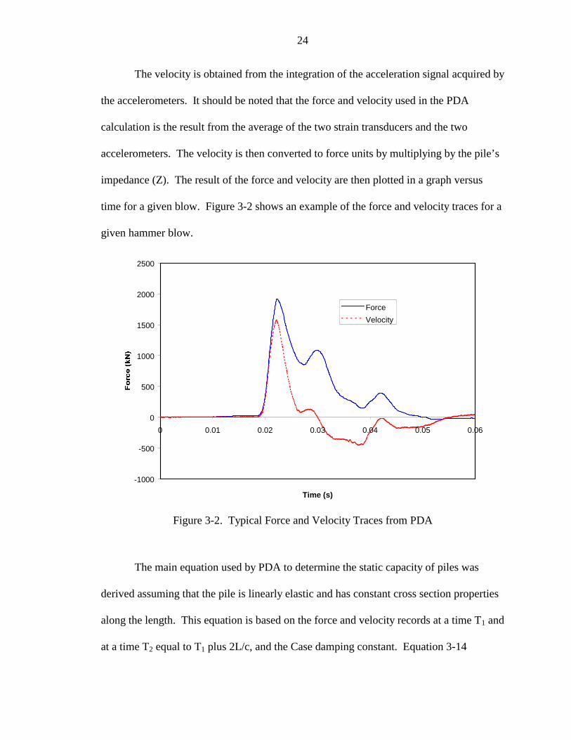
The velocity is obtained from the integration of the acceleration signal acquired by
the accelerometers. It should be noted that the force and velocity used in the PDA
calculation is the result from the average of the two strain transducers and the two
accelerometers. The velocity is then converted to force units by multiplying by the pile’s
impedance (Z). The result of the force and velocity are then plotted in a graph versus
time for a given blow. Figure 3-2 shows an example of the force and velocity traces for a
given hammer blow.
-1000
-500
0
500
1000
1500
2000
2500
0 0.01 0.02 0.03 0.04 0.05 0.06
Time (s)
Force
Velocity
Figure 3-2. Typical Force and Velocity Traces from PDA
The main equation used by PDA to determine the static capacity of piles was
derived assuming that the pile is linearly elastic and has constant cross section properties
along the length. This equation is based on the force and velocity records at a time T1 and
at a time T2 equal to T1 plus 2L/c, and the Case damping constant. Equation 3-14
25
presents the PDA equation for determining the static pile capacity. The reader is referred
to the PDA manual for detailed information and more thorough derivation.
( )[ ] ( )[ ]2
12
1 2211 ZVPJ
ZVPJRSP cc
−++−−= (3-14)
where RSP Total Static Capacity
Jc Case Damping Constant
P1,P2 Force at Time T1 and T2 Respectively
V1,V2 Velocities at Time T1 and T2 Respectively
Z Impedance
CAPWAP program
The Case Pile Wave Analysis Program (CAPWAP) is a computer program that
combines the wave equation’s pile and soil model with the Case method of forces and
velocities from PDA. The CAPWAP solution includes the static total resistance, skin
friction and toe bearing of the pile, in addition to the soil resistance distribution, damping
factors, and soil stiffness. The program calculates acceleration, velocities, displacements,
waves up, waves down and forces at all points along the pile.
The procedure used by CAPWAP includes inputting the force trace obtained from
PDA and adjust the soils parameters until the velocity trace obtained from PDA can be
recreated. It should be noticed that the opposite procedure (i.e. input velocity trace and
generate the force trace) can also be performed. When the match obtained is

26
unsatisfactory, it is necessary to modify the soil parameters, until reaching a satisfactory
match results. The process of running CAPWAP is considered an iterative one.
27
CHAPTER 4
UNIVERSITY OF FLORIDA PILE DATABASE
General Information and History
The University of Florida in conjunction with the Florida Department of
Transportation (FDOT) has developed a database on driven piles inside and outside the
state of Florida. This database, called PILEUF, is the result of many years of research to
predict pile capacity from static and dynamic means.
Originally, the database was on a Lotus 123 spreadsheet format. However, the
database information was transferred to a Microsoft Excel format for this research. By
doing the latter, the automatic tasks (macros) or links from Lotus 123 were eliminated.
Also, new pile information was obtained from the original geotechnical reports, as well as
new cases studied.
Currently, there are 242 piles in the database. Out of these 242 piles, 198 are
concrete piles (both square and round), 21 are steel pipe piles, and 9 are H-Piles. Table 4-
1 summarizes the number of piles, classification and diameter for the Florida cases while
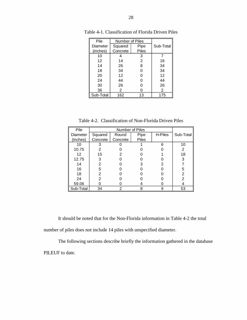
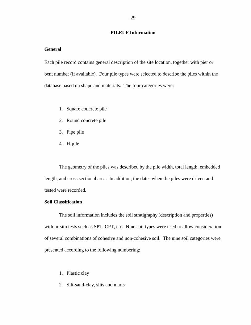
Table 4-2 summarizes the same information for the Non Florida cases.
The Florida State total includes 175 piles obtained from 60 sites and represents
218 cases. The difference between the number of piles and cases is due to the multiple
attempts to determine the same pile’s capacity. The Non-Florida total from Table 4-2
represents 22 sites. In this occasion the number of cases are equal to the number of piles.
28
Table 4-1. Classification of Florida Driven Piles
Pile Number of PilesDiameter Squared Pipe Sub-Total(inches) Concrete Piles
10 4 3 712 14 2 1614 26 8 3418 34 0 3420 12 0 1224 44 0 4430 26 0 2636 2 0 2
Sub-Total 162 13 175
Table 4-2. Classification of Non-Florida Driven Piles
Pile Number of PilesDiameter Squared Round Pipe H-Piles Sub-Total(inches) Concrete Concrete Piles
10 3 0 1 6 1010.75 2 0 0 0 2
12 15 2 0 1 1812.75 3 0 0 0 3
14 2 0 3 2 716 5 0 0 0 518 2 0 0 0 224 2 0 0 0 2
59.06 0 0 4 0 4Sub-Total 34 2 8 9 53
It should be noted that for the Non-Florida information in Table 4-2 the total
number of piles does not include 14 piles with unspecified diameter.
The following sections describe briefly the information gathered in the database
PILEUF to date.
29
PILEUF Information
General
Each pile record contains general description of the site location, together with pier or
bent number (if available). Four pile types were selected to describe the piles within the
database based on shape and materials. The four categories were:
1. Square concrete pile
2. Round concrete pile
3. Pipe pile
4. H-pile
The geometry of the piles was described by the pile width, total length, embedded
length, and cross sectional area. In addition, the dates when the piles were driven and
tested were recorded.
Soil Classification
The soil information includes the soil stratigraphy (description and properties)
with in-situ tests such as SPT, CPT, etc. Nine soil types were used to allow consideration
of several combinations of cohesive and non-cohesive soil. The nine soil categories were
presented according to the following numbering:
1. Plastic clay
2. Silt-sand-clay, silts and marls

30
3. Clean sand
4. Limestone, very shelly sands
5. Clayey sand
6. Sandy Clay
7. Silty clay
8. Rocks
9. Sandy gravel, tills
The original database combined the side and tip soil number to form a two-digit
code, in which the first digit is the side soil type and the second digit is the tip soil type.
Driving Information
The driving information includes the driving system type, hammer and pile weight
and manufacturer’s rated energy together with the efficiency of the hammer. Additional
information includes the dynamic modulus, wave speed and the pile impedance. If the
impedance was not available from CAPWAP or other results, it was calculated as EA/c.
The average set for EOD and BOR was taken as the inverse of the blow counts as near as
possible to the blow used in PDA or CAPWAP analysis, although it may represent an
average of the last foot of driving in some cases, if inch-by-inch information was not
available. A record of the depth of penetration and blows per foot (calculated for
penetration intervals less than one foot) facilitated the determination of set, knowing the
tip depth at the time of the blow.

31
Dynamic Data (CAPWAP and PDA)
The CAPWAP and PDA results were sometimes available only for EOD or BOR.
Furthermore, not all CAPWAP analyses have complete PDA results available or vice
versa. Having both results was not a requirement during the construction of the database.
The PDA results include date, RMX (maximum Case Static Resistance calculated
during the blow analysis) or other PDA calculated capacity as listed in the source report.
The database also presents the PDA Case damping used for calculating the Total Static
Resistance.
CAPWAP results include date, tip and friction capacities, total capacity, and Case
and Smith damping factors for side and tip, where the Case damping factors were
calculated from the Smith damping factors. The latter was performed by dividing the
Smith damping value by the impedance and multiplying the result by the side or tip
resistance.
Load Test Results
PILEUF contains load test information, measured at the top of the piles. It
includes the load in tons and settlements in inches at failure for a given criterion. The
failure criteria presented in the database are:
1. Davisson
2. Fuller-Hoy
3. DeBeer
4. FDOT
32
The database also includes the maximum load in tons from the static load test, in
addition to the date at which the load test was performed.
SPT94 Capacity
SPT94 (most recent version - SPT97) is a pile capacity prediction program. It is
based on the Research Bulletin 121 (RB-121), “Guidelines for use in the Soils
Investigation and Design of Foundations for Bridge Structures in the State of Florida”,
prepared by Schmertmann in 1967, and the research report “Design of Steel Pipe and H-
piles” prepared by Dr. Michael McVay et al in 1994. The method calculates pile capacity
based on N values obtained from the Standard Penetration Test. SPT94 is capable of
evaluating round and square concrete piles, H-piles, and steel pipe piles (open or close
end). It calculates an Estimated Davisson capacity by summing the Ultimate Side
Friction and 1/3 of the Ultimate End Bearing (Mobilized End Bearing) capacity of the
pile.
SPT94 predictions presented in PILEUF include the Ultimate Side Friction,
Ultimate Tip Capacity, Mobilized Tip Capacity, Ultimate Total Capacity, and Davisson’s
Capacity.
Other related information presented in the database is the input data for SPT94
program. It includes the layering and the soil properties (i.e. unit weight and SPT blow
count).
Gathering New Information
During the course of evaluating the eight dynamic method (See Chapter 3), some
extra information was necessary. In order to acquire it, it was required to restudy the
33
geotechnical reports from which the original information was obtained. Some of these
parameters are presented in the next sections.
Additional Required Information
Two parameters that were not found in the PILEUF database were the maximum
displacement and the maximum energy transfer to the pile. They were essential to obtain
the Paikowsky and Sakai capacities (See Chapter 3). Both, the maximum energy transfer
to the pile and the maximum displacement were obtained from the CAPWAP output
printout in the geotechnical reports.
Criteria for New Entries
As a general criterion, new entries in the database should be within the State of
Florida. Pile cases from outside the State of Florida were not considered in this study.
Because the evaluation of the dynamic methods was performed in correlation to the
Davisson capacity, new entries in the database should have the load test carried to the
point in which Davisson capacity could be determined. Other information required will
depend of the methods to be evaluated. The more information obtained for a particular
record, the more dynamic methods there are to be evaluated in relation to the Davisson
capacity.
34
CHAPTER 5
ASD AND LRFD CONCEPTS
Over the years, multiple design procedures have been developed which provide
satisfactory margins of safety. Safety in design is obtained when the material properties
exceed the demand put on them by any load or loads combination. Another way to
describe the same principle is that the resistance of the structure must exceed the effect of
the loads, i.e.:
Loads ofEffect Resistance≥ (5-1)
When a specific loading condition reaches its limit, failure occurs. Two general
states of interest to engineers are Strength and Service Limit. Strength Limit State
involves the total or partial collapse of the structure (i.e. bearing capacity failure, sliding,
and overall instability). On the other hand, Service Limit State only affects the function
of the structure under regular service loading conditions (i.e. excessive settlement and/or
lateral deflection, structural deterioration, etc).
Allowable Stress Design (ASD) Method
In geotechnical engineering, the ASD has been the primary method used in U.S.A.
ASD procedures are different for Service Limit and Strength Limit States. For the
Strength Limit State, safety is obtained in the foundation elements by restricting the
35
ultimate loads to values less than the ultimate resistance divided by a factor of safety,
(FS):
∑≥ in Q
FS
R(5-2)
where Rn Nominal Resistance
ΣQi Load Effect (Dead, Live and Environmental Loads)
FS Factor of Safety
For the Service Limit State, the deformations (i.e. settlements) are calculated
using the unfactored loads, and the values obtained are compared to the allowable
deformation for that structure.
Load Resistance Factor Design (LRFD) Method
The LRFD specifications as approved by AASHTO in 1994 recommend the use of
load(s) factors to account for uncertainty in the load(s) and a resistance(s) factor to
account for the uncertainty in the material resistance(s). This safety criterion can be
written as
∑= iin QR γηφ (5-3)
where φ Statistically Based Resistance Factor

36
Rn Nominal Resistance
η Load Modifier to Account for Effects of Ductility,
Redundancy and Operational Importance
γi Statistically Based Load Factor
Qi Load effect
Even though the LRFD method differs from the accustomed ASD procedure, it
has been widely approved by the geotechnical engineers. Some of the advantages and
disadvantages of the LRFD method over the ASD method are presented next (Withiam et
al., 1997).
Advantages of LRFD Over ASD
1. Account for variability in both resistance and load.
2. Achieves relatively uniform levels of safety based on the strength of soil and
rock for different limit states, foundation types, and design methods.
3. Provide more consistent levels of safety in the superstructure and substructure
when the same probabilities of failure are employed.
4. Using load and resistance factors provided in the code, no complex
probability and statistical analysis is required.
Limitation of LRFD
1. Implementation requires a change in design procedures for engineers
accustomed to ASD.
2. Resistance factors vary with design methods and are not constants.

37
3. The most rigorous method for developing and adjusting resistance factors to
meet individual situations requires availability of statistical data and
probabilistic design algorithms.
Calibration of LRFD
Calibration is defined as the process of assigning values to resistance factors and
load factors, which are indispensable for the LRFD approach. This process can be
performed by use of engineering judgement, fitting to other codes (e.g. ASD method), use
of reliability theory, or a combination of them. In the following sections these approaches
will be discussed.
Engineering Judgement
The calibration of a code using engineering judgement requires experience. Such
experience is usually obtained through years of engineering practice. Sometimes, using
such an approach results in certain level of conservatism with little validation. Also
under varying conditions where no experience exists both excessive conservatism or ever
unconservatism may develop.
Fitting ASD to LRFD
Fitting ASD to LRFD includes using parameters from LRFD (i.e. resistance
factor) that result in equivalent physical dimensions of a substructure or superstructure as
by ASD. It does not provide a better or more uniform margin of safety. In order to
calibrate the ASD method, the first step is to rewrite equations 5-2 and 5-3 as
38
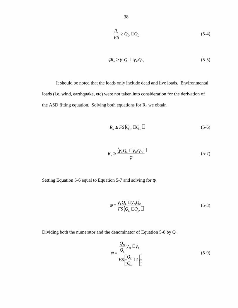
LDn QQ
FS
R +≥ (5-4)
DDLLn QQR γγφ +≥ (5-5)
It should be noted that the loads only include dead and live loads. Environmental
loads (i.e. wind, earthquake, etc) were not taken into consideration for the derivation of
the ASD fitting equation. Solving both equations for Rn we obtain
( )LDn QQFSR +≥ (5-6)
( )φ
γγ DDLLn
QQR
+≥ (5-7)
Setting Equation 5-6 equal to Equation 5-7 and solving for φ
( )DL
DDLL
QQFS
++= γγφ (5-8)
Dividing both the numerator and the denominator of Equation 5-8 by QL
+
+=
1L
D
LDL
D
Q
QFS
Q
Q γγφ (5-9)
39
Equation 5-9 is the resulting calibration equation for ASD fitting to the LRFD or
vice versa. For deep foundation design, the values of γD and γL recommended by LRFD
Highway Bridges Design Specifications (AASHTO, 1994) are 1.25 and 1.75 respectively.
The QD/QL definition and values will be presented in more detail in latter sections.
Calibration by fitting is recommended when there is insufficient statistical data to
perform a more sophisticated calibration by optimization. When statistical data is
available it is recommended to make use of reliability theory.
Reliability Calibration
Statistical data
In order to perform a reliability calibration for deep foundations (obtain resistance
factor, φ), such as piles and drilled shafts, the designer must have available statistical data
for the method of interest. This statistical data must include real or measured capacities
and the estimated or nominal capacities of the shafts. Next, the bias is defined as
n
mRi R
R=λ (5-10)
where λRi Bias Factor
Rm Measured Resistance
Rn Predicted (nominal) Resistance
The biases for all history cases using the same design procedure are subsequently
determined for the database and the values of mean, standard deviation and coefficient of
40
variance are then found. Equations 5-11, 5-12 and 5-13 are used for this purpose
(Withiam et al., 1997).
NRi
R∑=
λλ (5-11)
( )1
2
−−
= ∑N
TRiR
λλσ (5-12)
R
RRCOV
λσ= (5-13)
where λR Average Resistance Bias Factor
N Number of Cases
σR Resistance Standard Deviation
COVR Resistance Coefficient of Variance
For calibrations of the methods that predict driven pile capacity, the values of the
measured resistance (Rm) were obtained from in-situ load test employing the Davisson’s
capacity. The nominal resistances (Rn) were obtained from the various dynamic
equations under study (Chapter 3).
41
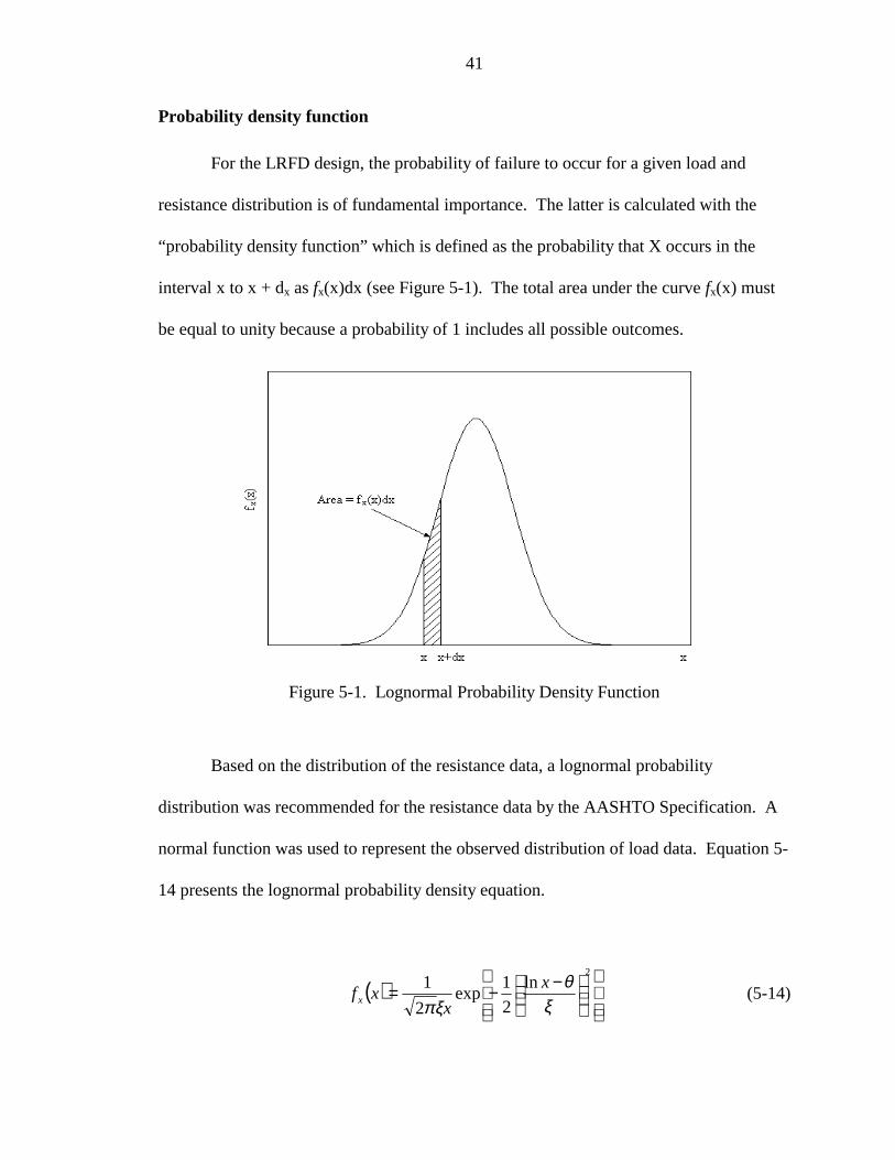
Probability density function
For the LRFD design, the probability of failure to occur for a given load and
resistance distribution is of fundamental importance. The latter is calculated with the
“probability density function” which is defined as the probability that X occurs in the
interval x to x + dx as fx(x)dx (see Figure 5-1). The total area under the curve fx(x) must
be equal to unity because a probability of 1 includes all possible outcomes.
Figure 5-1. Lognormal Probability Density Function
Based on the distribution of the resistance data, a lognormal probability
distribution was recommended for the resistance data by the AASHTO Specification. A
normal function was used to represent the observed distribution of load data. Equation 5-
14 presents the lognormal probability density equation.
( )
−−=2
ln
2
1exp
2
1
ξθ
ξπx
xxfx (5-14)
42
In Equation 5-14 the values of θ and ζ are the lognormal mean and lognormal
standard deviation respectively,
+= 2
22 1ln
R
R
λσξ (5-15)
2
2
1ln ξλθ −= R (5-16)
Where σR and λR are the standard deviation and the mean of the resistance as
defined in prior sections.
LRFD components
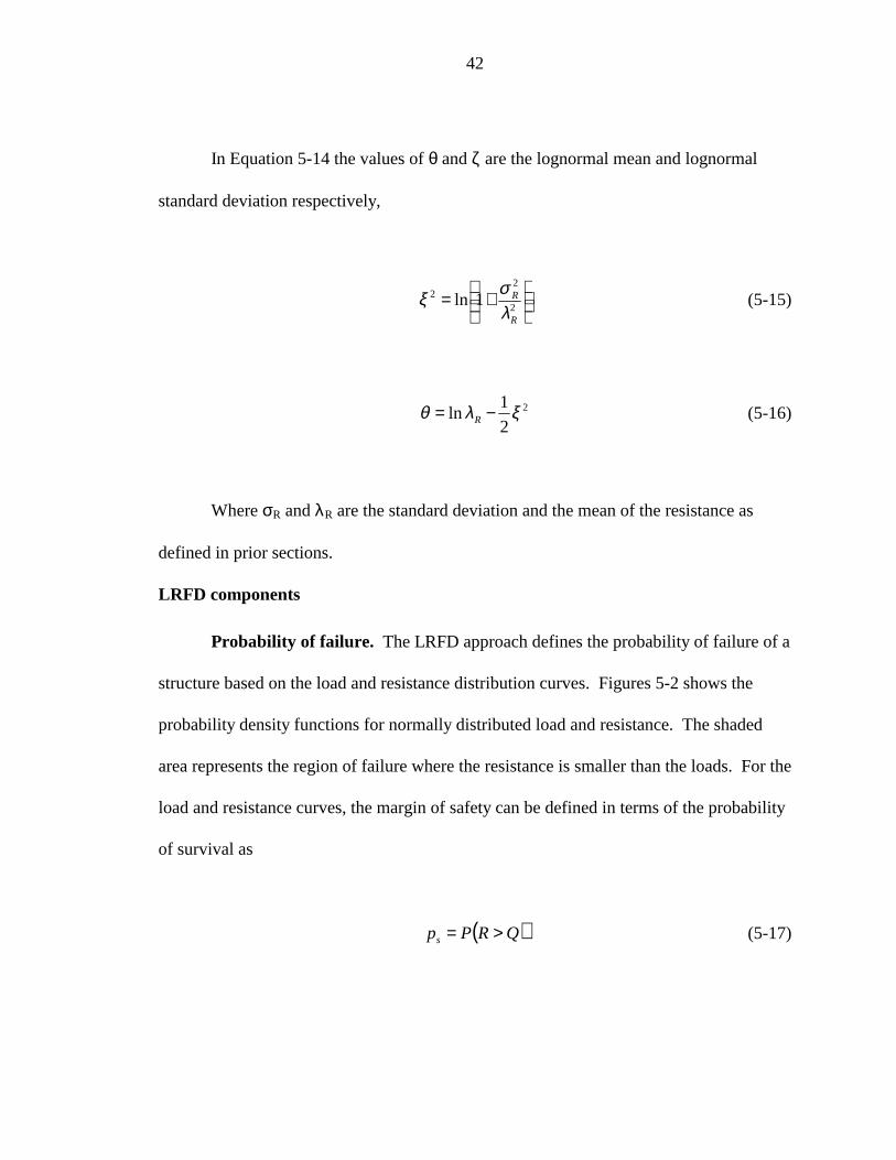
Probability of failure. The LRFD approach defines the probability of failure of a
structure based on the load and resistance distribution curves. Figures 5-2 shows the
probability density functions for normally distributed load and resistance. The shaded
area represents the region of failure where the resistance is smaller than the loads. For the
load and resistance curves, the margin of safety can be defined in terms of the probability
of survival as
( )QRPps >= (5-17)
43
Figure 5-2. Probability Density Functions for Normally Distributed Load and Resistance
And the probability of failure, pf may be represented as
)(1 QRPpp sf <=−= (5-18)
where the right hand of Equation 5-18 represents the probability, P, that R is less than Q.
It should be noted that the probability of failure can not be calculated directly
from the shaded area in Figure 5-2. That area represents a mixture of areas from the load
and resistance distribution curves that have different ratios of standard deviation to mean
values. To evaluate the probability of failure, a single combined probability density curve
function of the resistance and load may developed based on a normal distribution, i.e.
( ) QRQRg −=, (5-19)
If a lognormal distribution is used the limit state function g(R,Q) can be written as
44
( )QRQRQRg ln)ln()ln(),( =−= (5-20)
For both Equation 5-19 and 5-20 the limit state is reached when R=Q and failure
will occurs when g(R,Q)<0.
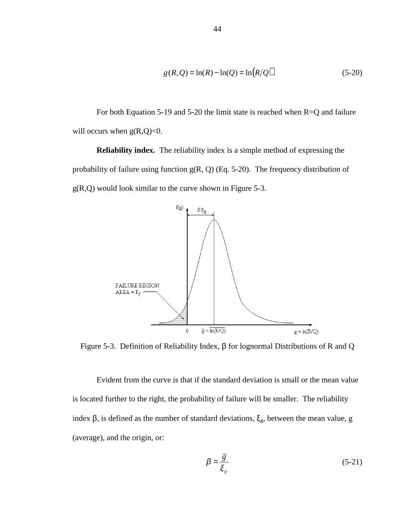
Reliability index. The reliability index is a simple method of expressing the
probability of failure using function g(R, Q) (Eq. 5-20). The frequency distribution of
g(R,Q) would look similar to the curve shown in Figure 5-3.
Figure 5-3. Definition of Reliability Index, β for lognormal Distributions of R and Q
Evident from the curve is that if the standard deviation is small or the mean value
is located further to the right, the probability of failure will be smaller. The reliability
index β, is defined as the number of standard deviations, ξg, between the mean value, g
(average), and the origin, or:
g
g
ξβ = (5-21)
45
If the resistance, R, and load, Q, are both lognormally distributed random
variables and are statistically independent, it can be shown that the mean values of g(R,
Q) is
++
=2
2
1
1ln
R
Q
COV
COV
Q
Rg (5-22)
and its standard deviation is
( )( )[ ]22 11ln QRg COVCOV ++=ξ (5-23)
Substituting Equations 5-22 and 5-23 into Equation 5-21, the relationship for the
reliability index, β, can be expressed as
( ) ( ) ( )[ ]( )( )[ ]22
22
11ln
1/1ln
QR
RQ
COVCOV
COVCOVQR
++
++=β (5-24)
Equation 5-24 is very convenient because it depends only on statistical data and
not on the distribution of the combined function g(R, Q). A very precise definition of
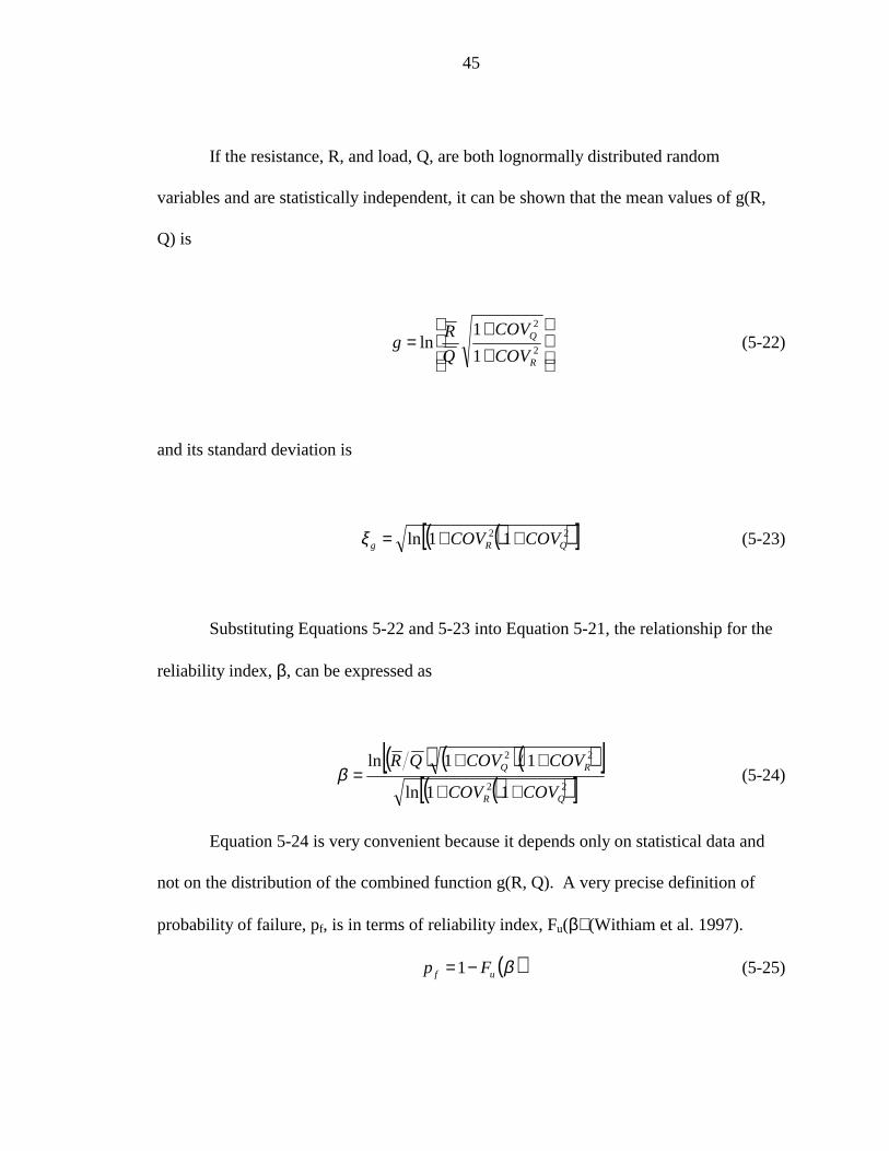
probability of failure, pf, is in terms of reliability index, Fu(β) (Withiam et al. 1997).
( )βuf Fp −=1 (5-25)
46
Figure 5-4. Reliability Definition Based on Standard Normal Probability DensityFunction
In the latter equation, Fu(x) is the standard normal cumulative distribution
function.
( ) dxxFu
−−= ∫
∞2
2
1exp
2
11
β πβ (5-26)
A graphical representation of Equation 5-26 is presented in Figure 5-4. The
shaded area in Figure 5-4 represents the probability of failure, pf, to achieve a target
reliability index, βT.
47
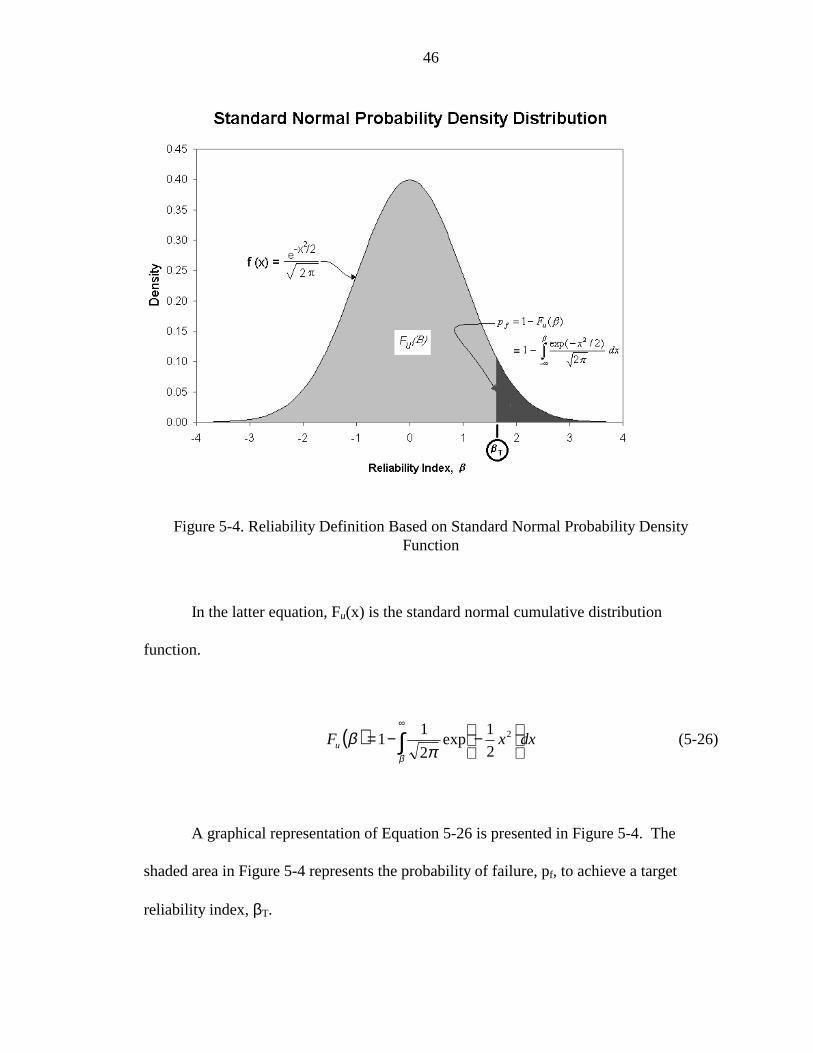
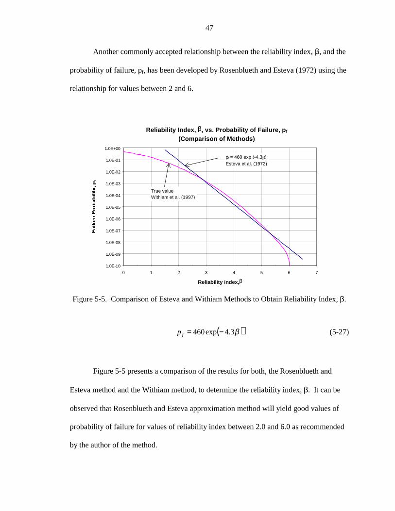
Another commonly accepted relationship between the reliability index, β, and the
probability of failure, pf, has been developed by Rosenblueth and Esteva (1972) using the
relationship for values between 2 and 6.
Reliability Index, β, vs. Probability of Failure, p f
(Comparison of Methods)
1.0E-10
1.0E-09
1.0E-08
1.0E-07
1.0E-06
1.0E-05
1.0E-04
1.0E-03
1.0E-02
1.0E-01
1.0E+00
0 1 2 3 4 5 6 7
Reliability index, β
pf = 460 exp (-4.3β)Esteva et al. (1972)
True valueWithiam et al. (1997)
Figure 5-5. Comparison of Esteva and Withiam Methods to Obtain Reliability Index, β.
( )β3.4exp460 −=fp (5-27)
Figure 5-5 presents a comparison of the results for both, the Rosenblueth and
Esteva method and the Withiam method, to determine the reliability index, β. It can be
observed that Rosenblueth and Esteva approximation method will yield good values of
probability of failure for values of reliability index between 2.0 and 6.0 as recommended
by the author of the method.
48
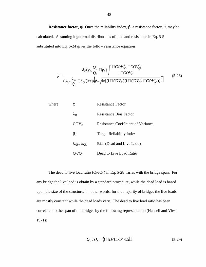
Resistance factor, φ. Once the reliability index, β, a resistance factor, φ, may be
calculated. Assuming lognormal distributions of load and resistance in Eq. 5-5
substituted into Eq. 5-24 gives the follow resistance equation
( ))]1)(1ln[(exp)(
1
1)(
222
2
22
QLQDRTQLL
DQD
R
QLQDL
L
DDR
COVCOVCOVQ
QCOV
COVCOV
Q
Q
++++
+++
+=
βλλ
γγλφ (5-28)
where φ Resistance Factor
λR Resistance Bias Factor
COVR Resistance Coefficient of Variance
βT Target Reliability Index
λQD, λQL Bias (Dead and Live Load)
QD/QL Dead to Live Load Ratio
The dead to live load ratio (QD/QL) in Eq. 5-28 varies with the bridge span. For
any bridge the live load is obtain by a standard procedure, while the dead load is based
upon the size of the structure. In other words, for the majority of bridges the live loads
are mostly constant while the dead loads vary. The dead to live load ratio has been
correlated to the span of the bridges by the following representation (Hansell and Viest,
1971):
( )( )LIMQQ LD 0132.01/ += (5-29)
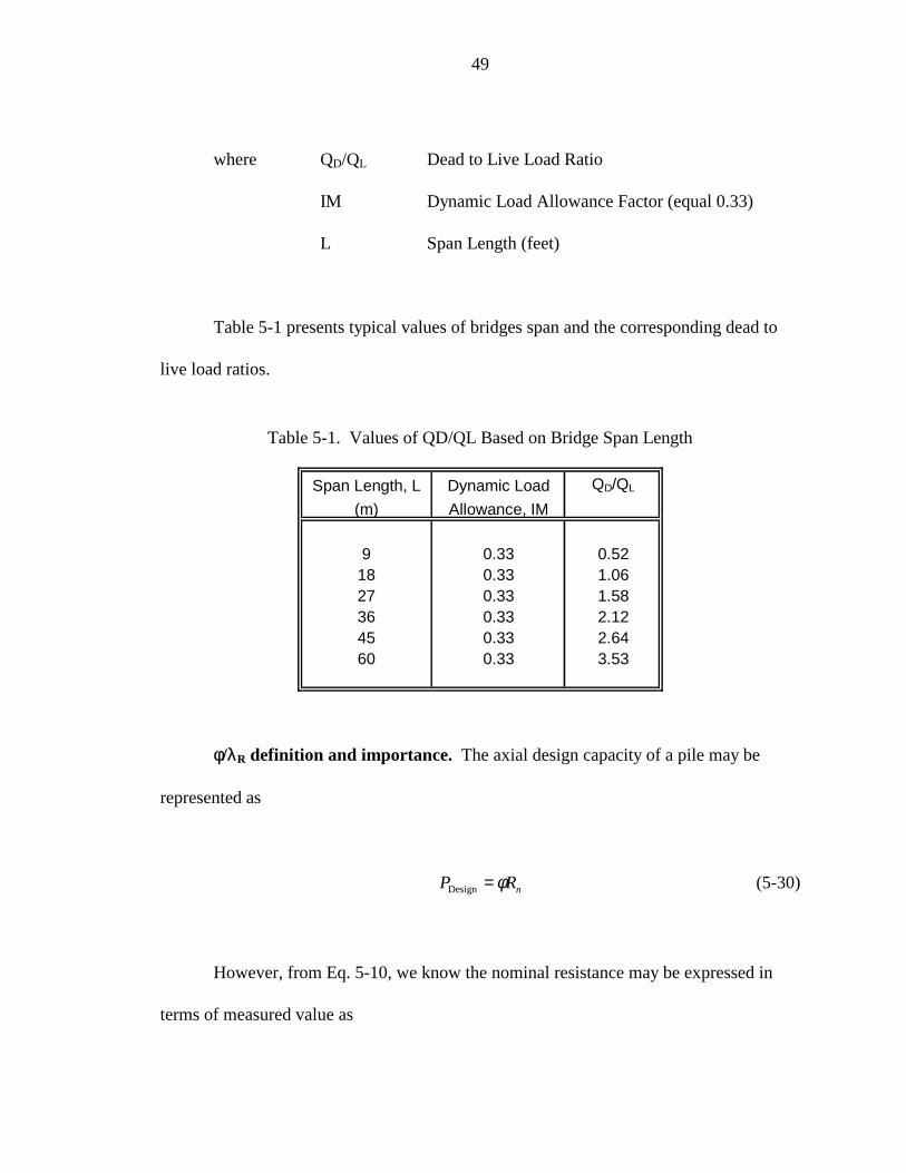
49
where QD/QL Dead to Live Load Ratio
IM Dynamic Load Allowance Factor (equal 0.33)
L Span Length (feet)
Table 5-1 presents typical values of bridges span and the corresponding dead to
live load ratios.
Table 5-1. Values of QD/QL Based on Bridge Span Length
Span Length, L Dynamic Load QD/QL
(m) Allowance, IM
9 0.33 0.5218 0.33 1.0627 0.33 1.5836 0.33 2.1245 0.33 2.6460 0.33 3.53
φ/λR definition and importance. The axial design capacity of a pile may be
represented as
nRP φ=Design (5-30)
However, from Eq. 5-10, we know the nominal resistance may be expressed in
terms of measured value as
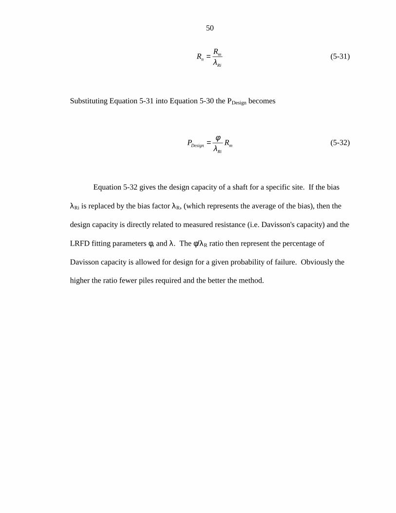
50
Ri
mn
RR
λ= (5-31)
Substituting Equation 5-31 into Equation 5-30 the PDesign becomes
mRi
Design RPλφ= (5-32)
Equation 5-32 gives the design capacity of a shaft for a specific site. If the bias
λRi is replaced by the bias factor λR, (which represents the average of the bias), then the
design capacity is directly related to measured resistance (i.e. Davisson's capacity) and the
LRFD fitting parameters φ, and λ. The φ/λR ratio then represent the percentage of
Davisson capacity is allowed for design for a given probability of failure. Obviously the
higher the ratio fewer piles required and the better the method.
51
CHAPTER 6
LRFD DATA PRESENTATION AND ANALYSIS
Data Reduction
Prior to determine the LRFD for each dynamic method, a simple statistical
analysis was performed. For all the dynamic methods, graphs of measured capacity
(Davisson Capacity) related to the estimated capacity at End of Drive (EOD) and
Beginning of Restrike (BOR) were constructed. The number of cases for each method
was determined based on the availability of parameters needed to obtain the estimated
capacity for the corresponding method. The statistic and some of the LRFD results
(tables & graphs) from each method are contained within separated Appendices (i.e.
Appendix A for all CAPWAP Procedure results, Appendix B for all PDA results,
Appendix C for Paikowsky’s Energy Method results, etc…)
Figures 6-1 and 6-2 present the plots for the PDA at BOR. Figure 6-1 presents a
simple graph of PDA BOR capacity versus Davisson Capacity. A line with slope equal
45 degrees has been drawn to facilitate the comparison between the two methods of
determining pile capacity. A regression line with the corresponding equation and R2 is
shown in the plot. This latter graph is ideal to visually determine how scattered the
predictions are for each method. The second graph (Figure 6-2, PDA at BOR) presents
the ratio of measured to predicted capacity on the vertical axis and the measured
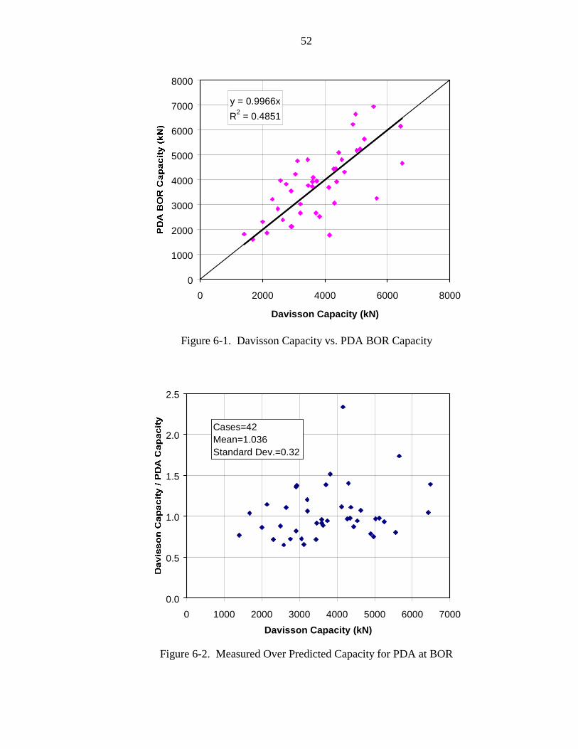
52
y = 0.9966x
R2 = 0.4851
0
1000
2000
3000
4000
5000
6000
7000
8000
0 2000 4000 6000 8000
Davisson Capacity (kN)
Figure 6-1. Davisson Capacity vs. PDA BOR Capacity
0.0
0.5
1.0
1.5
2.0
2.5
0 1000 2000 3000 4000 5000 6000 7000
Davisson Capacity (kN)
Cases=42Mean=1.036Standard Dev.=0.32
Figure 6-2. Measured Over Predicted Capacity for PDA at BOR
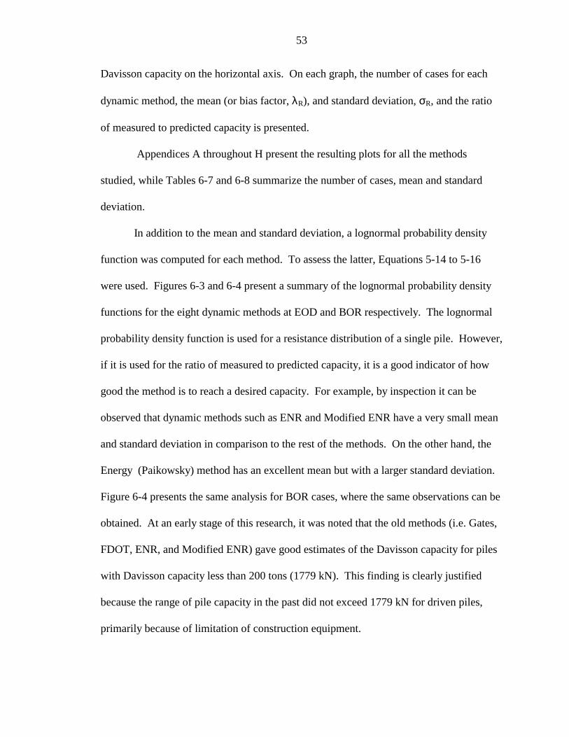
53
Davisson capacity on the horizontal axis. On each graph, the number of cases for each
dynamic method, the mean (or bias factor, λR), and standard deviation, σR, and the ratio
of measured to predicted capacity is presented.
Appendices A throughout H present the resulting plots for all the methods
studied, while Tables 6-7 and 6-8 summarize the number of cases, mean and standard
deviation.
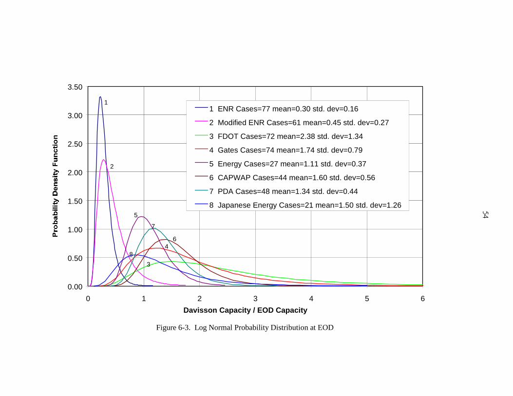
In addition to the mean and standard deviation, a lognormal probability density
function was computed for each method. To assess the latter, Equations 5-14 to 5-16
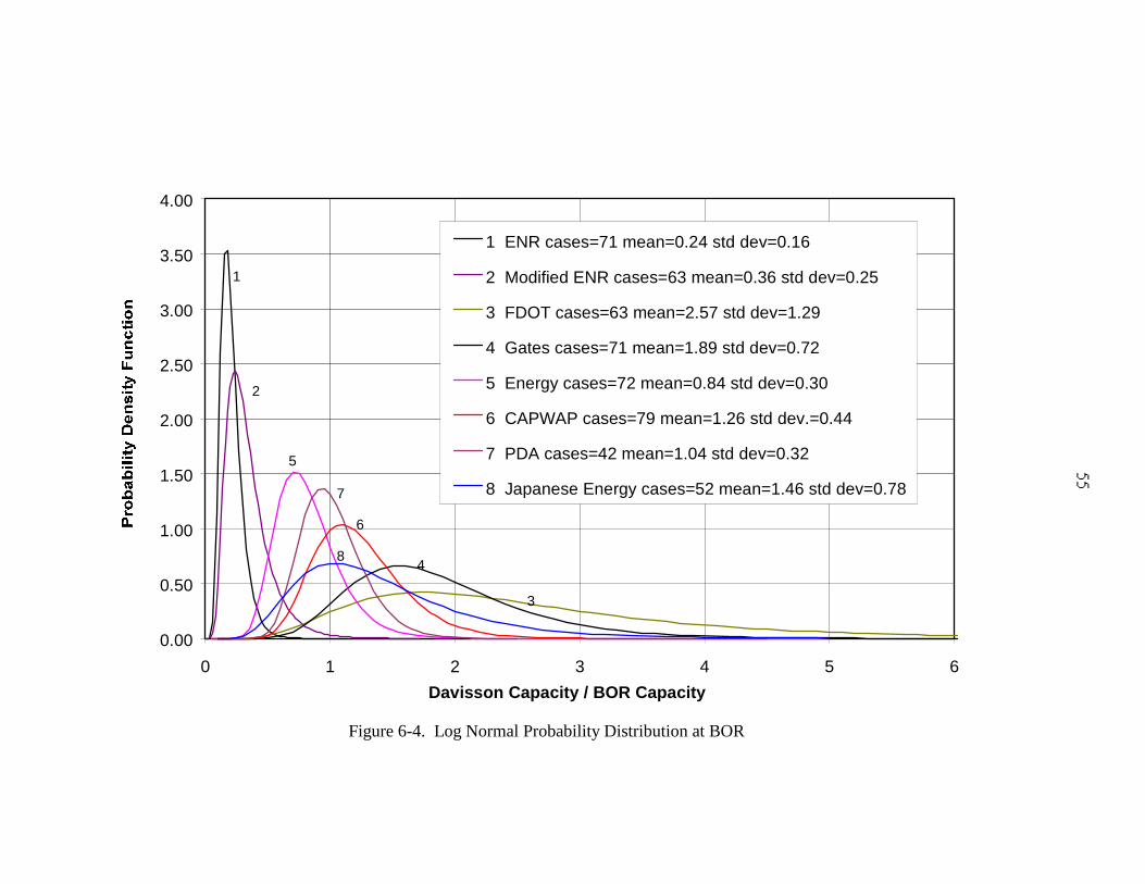
were used. Figures 6-3 and 6-4 present a summary of the lognormal probability density
functions for the eight dynamic methods at EOD and BOR respectively. The lognormal
probability density function is used for a resistance distribution of a single pile. However,
if it is used for the ratio of measured to predicted capacity, it is a good indicator of how
good the method is to reach a desired capacity. For example, by inspection it can be
observed that dynamic methods such as ENR and Modified ENR have a very small mean
and standard deviation in comparison to the rest of the methods. On the other hand, the
Energy (Paikowsky) method has an excellent mean but with a larger standard deviation.
Figure 6-4 presents the same analysis for BOR cases, where the same observations can be
obtained. At an early stage of this research, it was noted that the old methods (i.e. Gates,
FDOT, ENR, and Modified ENR) gave good estimates of the Davisson capacity for piles
with Davisson capacity less than 200 tons (1779 kN). This finding is clearly justified
because the range of pile capacity in the past did not exceed 1779 kN for driven piles,
primarily because of limitation of construction equipment.
0.00
0.50
1.00
1.50
2.00
2.50
3.00
3.50
0 1 2 3 4 5 6
Davisson Capacity / EOD Capacity
1 ENR Cases=77 mean=0.30 std. dev=0.16
2 Modified ENR Cases=61 mean=0.45 std. dev=0.27
3 FDOT Cases=72 mean=2.38 std. dev=1.34
4 Gates Cases=74 mean=1.74 std. dev=0.79
5 Energy Cases=27 mean=1.11 std. dev=0.37
6 CAPWAP Cases=44 mean=1.60 std. dev=0.56
7 PDA Cases=48 mean=1.34 std. dev=0.44
8 Japanese Energy Cases=21 mean=1.50 std. dev=1.26
6
7
2
1
3
4
5
8
Figure 6-3. Log Normal Probability Distribution at EOD
0.00
0.50
1.00
1.50
2.00
2.50
3.00
3.50
4.00
0 1 2 3 4 5 6
Davisson Capacity / BOR Capacity
1 ENR cases=71 mean=0.24 std dev=0.16
2 Modified ENR cases=63 mean=0.36 std dev=0.25
3 FDOT cases=63 mean=2.57 std dev=1.29
4 Gates cases=71 mean=1.89 std dev=0.72
5 Energy cases=72 mean=0.84 std dev=0.30
6 CAPWAP cases=79 mean=1.26 std dev.=0.44
7 PDA cases=42 mean=1.04 std dev=0.32
8 Japanese Energy cases=52 mean=1.46 std dev=0.78
5
2
1
6
3
4
7
8
Figure 6-4. Log Normal Probability Distribution at BOR
56
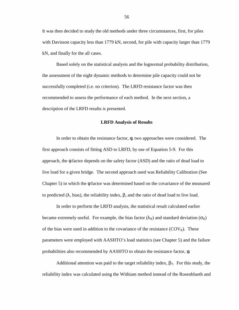
It was then decided to study the old methods under three circumstances, first, for piles
with Davisson capacity less than 1779 kN, second, for pile with capacity larger than 1779
kN, and finally for the all cases.
Based solely on the statistical analysis and the lognormal probability distribution,
the assessment of the eight dynamic methods to determine pile capacity could not be
successfully completed (i.e. no criterion). The LRFD resistance factor was then
recommended to assess the performance of each method. In the next section, a
description of the LRFD results is presented.
LRFD Analysis of Results
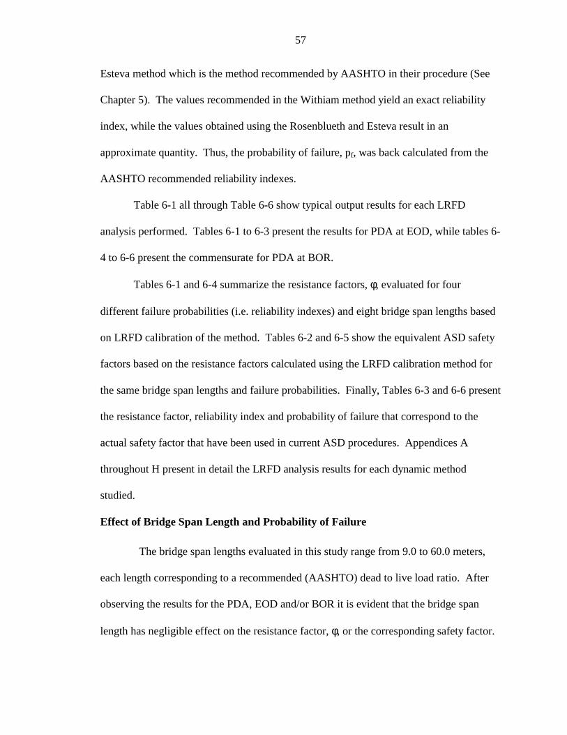
In order to obtain the resistance factor, φ, two approaches were considered. The
first approach consists of fitting ASD to LRFD, by use of Equation 5-9. For this
approach, the φ factor depends on the safety factor (ASD) and the ratio of dead load to
live load for a given bridge. The second approach used was Reliability Calibration (See
Chapter 5) in which the φ factor was determined based on the covariance of the measured
to predicted (λ, bias), the reliability index, β, and the ratio of dead load to live load.
In order to perform the LRFD analysis, the statistical result calculated earlier
became extremely useful. For example, the bias factor (λR) and standard deviation (σR)
of the bias were used in addition to the covariance of the resistance (COVR). These
parameters were employed with AASHTO’s load statistics (see Chapter 5) and the failure
probabilities also recommended by AASHTO to obtain the resistance factor, φ.
Additional attention was paid to the target reliability index, βT. For this study, the
reliability index was calculated using the Withiam method instead of the Rosenblueth and
57
Esteva method which is the method recommended by AASHTO in their procedure (See
Chapter 5). The values recommended in the Withiam method yield an exact reliability
index, while the values obtained using the Rosenblueth and Esteva result in an
approximate quantity. Thus, the probability of failure, pf, was back calculated from the
AASHTO recommended reliability indexes.
Table 6-1 all through Table 6-6 show typical output results for each LRFD
analysis performed. Tables 6-1 to 6-3 present the results for PDA at EOD, while tables 6-
4 to 6-6 present the commensurate for PDA at BOR.
Tables 6-1 and 6-4 summarize the resistance factors, φ, evaluated for four
different failure probabilities (i.e. reliability indexes) and eight bridge span lengths based
on LRFD calibration of the method. Tables 6-2 and 6-5 show the equivalent ASD safety
factors based on the resistance factors calculated using the LRFD calibration method for
the same bridge span lengths and failure probabilities. Finally, Tables 6-3 and 6-6 present
the resistance factor, reliability index and probability of failure that correspond to the
actual safety factor that have been used in current ASD procedures. Appendices A
throughout H present in detail the LRFD analysis results for each dynamic method
studied.
Effect of Bridge Span Length and Probability of Failure
The bridge span lengths evaluated in this study range from 9.0 to 60.0 meters,
each length corresponding to a recommended (AASHTO) dead to live load ratio. After
observing the results for the PDA, EOD and/or BOR it is evident that the bridge span
length has negligible effect on the resistance factor, φ, or the corresponding safety factor.
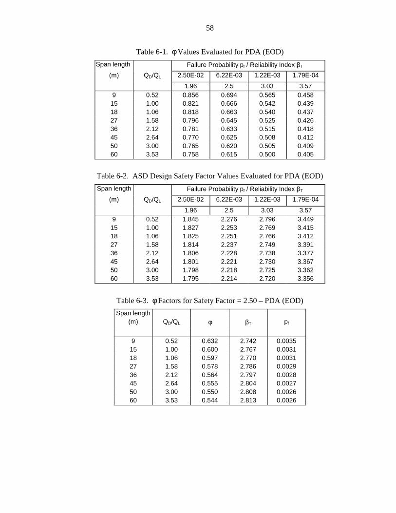
58
Table 6-1. φ Values Evaluated for PDA (EOD)
Span length Failure Probability pf / Reliability Index βΤ
(m) QD/QL 2.50E-02 6.22E-03 1.22E-03 1.79E-04
1.96 2.5 3.03 3.579 0.52 0.856 0.694 0.565 0.45815 1.00 0.821 0.666 0.542 0.43918 1.06 0.818 0.663 0.540 0.43727 1.58 0.796 0.645 0.525 0.42636 2.12 0.781 0.633 0.515 0.41845 2.64 0.770 0.625 0.508 0.41250 3.00 0.765 0.620 0.505 0.40960 3.53 0.758 0.615 0.500 0.405
Table 6-2. ASD Design Safety Factor Values Evaluated for PDA (EOD)
Span length Failure Probability pf / Reliability Index βΤ
(m) QD/QL 2.50E-02 6.22E-03 1.22E-03 1.79E-04
1.96 2.5 3.03 3.579 0.52 1.845 2.276 2.796 3.44915 1.00 1.827 2.253 2.769 3.41518 1.06 1.825 2.251 2.766 3.41227 1.58 1.814 2.237 2.749 3.39136 2.12 1.806 2.228 2.738 3.37745 2.64 1.801 2.221 2.730 3.36750 3.00 1.798 2.218 2.725 3.36260 3.53 1.795 2.214 2.720 3.356
Table 6-3. φ Factors for Safety Factor = 2.50 – PDA (EOD)
Span length(m) QD/QL φ βΤ pf
9 0.52 0.632 2.742 0.003515 1.00 0.600 2.767 0.003118 1.06 0.597 2.770 0.003127 1.58 0.578 2.786 0.002936 2.12 0.564 2.797 0.002845 2.64 0.555 2.804 0.002750 3.00 0.550 2.808 0.002660 3.53 0.544 2.813 0.0026
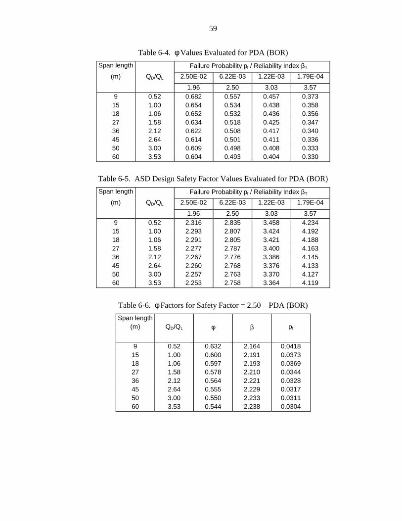
59
Table 6-4. φ Values Evaluated for PDA (BOR)
Span length Failure Probability pf / Reliability Index βΤ
(m) QD/QL 2.50E-02 6.22E-03 1.22E-03 1.79E-04
1.96 2.50 3.03 3.579 0.52 0.682 0.557 0.457 0.37315 1.00 0.654 0.534 0.438 0.35818 1.06 0.652 0.532 0.436 0.35627 1.58 0.634 0.518 0.425 0.34736 2.12 0.622 0.508 0.417 0.34045 2.64 0.614 0.501 0.411 0.33650 3.00 0.609 0.498 0.408 0.33360 3.53 0.604 0.493 0.404 0.330
Table 6-5. ASD Design Safety Factor Values Evaluated for PDA (BOR)
Span length Failure Probability pf / Reliability Index βΤ
(m) QD/QL 2.50E-02 6.22E-03 1.22E-03 1.79E-04
1.96 2.50 3.03 3.579 0.52 2.316 2.835 3.458 4.23415 1.00 2.293 2.807 3.424 4.19218 1.06 2.291 2.805 3.421 4.18827 1.58 2.277 2.787 3.400 4.16336 2.12 2.267 2.776 3.386 4.14545 2.64 2.260 2.768 3.376 4.13350 3.00 2.257 2.763 3.370 4.12760 3.53 2.253 2.758 3.364 4.119
Table 6-6. φ Factors for Safety Factor = 2.50 – PDA (BOR)
Span length(m) QD/QL φ β pf
9 0.52 0.632 2.164 0.041815 1.00 0.600 2.191 0.037318 1.06 0.597 2.193 0.036927 1.58 0.578 2.210 0.034436 2.12 0.564 2.221 0.032845 2.64 0.555 2.229 0.031750 3.00 0.550 2.233 0.031160 3.53 0.544 2.238 0.0304
60
At a target reliability index of 2.5 for both EOD and BOR, the φ factor decreases only
6.8% and the safety factor decreases only 1.6% when the span length increased from 15.0
meters to 50.0 meters. The latter phenomenon was observed throughout all the methods
evaluated. Thus, for practical purposes the rest of LRFD analysis results are summarized
for a 27 meters bridge span length.
In terms of the probability of failure, pf, the increase in probability of failure was
directly related to a decrease in reliability index, β, and a diminishment in the resistance
factor, φ. This effect could be easily understood, because lowering the probability of
failure for a given structure should be accompanied by a reduction of the resistance factor,
which means, penalizing the structure resistance and producing a more conservative
design. Different to the effect of the bridge span length, the reliability index has a big
influence in the resistance factor φ, and the equivalent safety factor. The relation of
φ factor and reliability index, β, is inversely proportional and linear. For piles AASHTO
recommends a reliability index, β, of 2.0 to 2.5.
Level of Conservatism and Accuracy Indicators
Similar analyses as those presented in Tables 6-1 to 6-6 were performed for each
of the eight dynamic methods, as well as breaking the old methods in terms of Davisson
capacity less than 1779 kN and larger than 1779 kN. A summary of the results is
presented in Tables 6-7 and 6-8 for EOD and BOR respectively.
The results show that the higher the bias factor λR, for a given method the higher
the resulting resistance factor will be. For example, for CAPWAP at BOR the mean is
equal to 1.260 and φ is equal to 0.58 (for β = 2.50) while FDOT method shows a mean
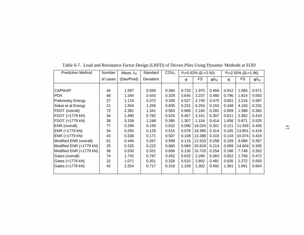
Table 6-7. Load and Resistance Factor Design (LRFD) of Driven Piles Using Dynamic Methods at EOD
Prediction Method Number Mean, λR Standard COVR Pf=0.62% (βT=2.50) Pf=2.50% (βT=1.96)
of cases (Dav/Pred) Deviation φ FS φ/λR φ FS φ/λR
CAPWAP 44 1.597 0.559 0.350 0.733 1.970 0.459 0.912 1.584 0.571PDA 48 1.344 0.443 0.329 0.645 2.237 0.480 0.796 1.814 0.592Paikowsky Energy 27 1.110 0.372 0.335 0.527 2.740 0.475 0.651 2.216 0.587Sakai et al Energy 21 1.504 1.256 0.835 0.231 6.254 0.153 0.348 4.150 0.231FDOT (overall) 72 2.381 1.341 0.563 0.669 2.160 0.281 0.909 1.588 0.382FDOT (<1779 kN) 34 1.490 0.782 0.525 0.457 3.161 0.307 0.611 2.362 0.410FDOT (>1779 kN) 38 3.158 1.248 0.395 1.307 1.104 0.414 1.658 0.871 0.525ENR (overall) 77 0.299 0.159 0.532 0.090 16.024 0.301 0.121 11.935 0.405ENR (<1779 kN) 34 0.250 0.129 0.515 0.078 18.395 0.314 0.105 13.801 0.419ENR (>1779 kN) 43 0.338 0.171 0.507 0.108 13.388 0.319 0.143 10.074 0.424Modified ENR (overall) 61 0.446 0.267 0.599 0.115 12.533 0.258 0.159 9.086 0.357Modified ENR (<1779 kN) 25 0.325 0.222 0.683 0.069 20.818 0.214 0.099 14.604 0.305Modified ENR (>1779 kN) 36 0.530 0.321 0.606 0.135 10.720 0.254 0.186 7.749 0.352Gates (overall) 74 1.742 0.787 0.452 0.633 2.280 0.363 0.822 1.756 0.472Gates (<1779 kN) 32 1.071 0.351 0.328 0.515 2.802 0.481 0.635 2.272 0.593Gates (>1779 kN) 42 2.254 0.717 0.318 1.109 1.302 0.492 1.361 1.061 0.604
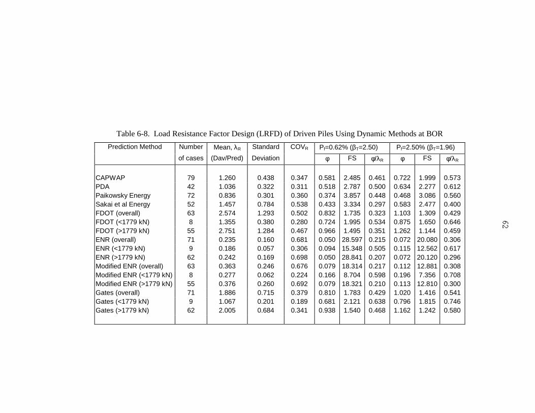
Table 6-8. Load Resistance Factor Design (LRFD) of Driven Piles Using Dynamic Methods at BOR
Prediction Method Number Mean, λR Standard COVR Pf=0.62% (βT=2.50) Pf=2.50% (βT=1.96)
of cases (Dav/Pred) Deviation φ FS φ/λR φ FS φ/λR
CAPWAP 79 1.260 0.438 0.347 0.581 2.485 0.461 0.722 1.999 0.573PDA 42 1.036 0.322 0.311 0.518 2.787 0.500 0.634 2.277 0.612Paikowsky Energy 72 0.836 0.301 0.360 0.374 3.857 0.448 0.468 3.086 0.560Sakai et al Energy 52 1.457 0.784 0.538 0.433 3.334 0.297 0.583 2.477 0.400FDOT (overall) 63 2.574 1.293 0.502 0.832 1.735 0.323 1.103 1.309 0.429FDOT (<1779 kN) 8 1.355 0.380 0.280 0.724 1.995 0.534 0.875 1.650 0.646FDOT (>1779 kN) 55 2.751 1.284 0.467 0.966 1.495 0.351 1.262 1.144 0.459ENR (overall) 71 0.235 0.160 0.681 0.050 28.597 0.215 0.072 20.080 0.306ENR (<1779 kN) 9 0.186 0.057 0.306 0.094 15.348 0.505 0.115 12.562 0.617ENR (>1779 kN) 62 0.242 0.169 0.698 0.050 28.841 0.207 0.072 20.120 0.296Modified ENR (overall) 63 0.363 0.246 0.676 0.079 18.314 0.217 0.112 12.881 0.308Modified ENR (<1779 kN) 8 0.277 0.062 0.224 0.166 8.704 0.598 0.196 7.356 0.708Modified ENR (>1779 kN) 55 0.376 0.260 0.692 0.079 18.321 0.210 0.113 12.810 0.300Gates (overall) 71 1.886 0.715 0.379 0.810 1.783 0.429 1.020 1.416 0.541Gates (<1779 kN) 9 1.067 0.201 0.189 0.681 2.121 0.638 0.796 1.815 0.746Gates (>1779 kN) 62 2.005 0.684 0.341 0.938 1.540 0.468 1.162 1.242 0.580
63
and resistance factor of 2.574 and 0.97 respectively for the same reliability index. This
effect could be explained in terms of the bias factors meaning. As defined in the
preceding chapters, the bias factor is the ratio of measured to predicted capacity. Then, a
large bias factor means a very conservative method and the result is a higher resistance
factor.
Although the resistance factor is a good qualitative method to determine the
degree of conservatism or unconservatism, it does not indicate the accuracy of the
method. The combination of both, mean and standard deviation through the COVR (i.e.
ratio of standard deviation to the mean or bias) has proved to be a good indicator of the
accuracy of the methods. Under this criterion, the new methods such as PDA,
Paikowsky, and CAPWAP have the best accuracy, while ENR and modified ENR have
the worst accuracy.
φ/λR Ratio
The efficiency or performance of the dynamic methods can be evaluated by the
ratio of φ/λR, indicating the percentage of the measured Davisson capacity that can be
utilized for design to reach a pre-defined structure reliability. It must be remembered that
the average bias factor λR is an average of each pile bias, therefore, φ/λR ratio is an
“approximated” percentage of the measured Davisson capacity. The latter consideration
makes the φ/λR ratio remarkably valuable from an economic point of view. The higher
the φ/λR ratio the more cost effective the method is.
64
Methods comparison
From Table 6-7 (LRFD Results for Dynamic Methods at EOD) it can be observed
that for the reliability index, β = 2.50, the φ/λR values for the new methods such as
CAPWAP (φ/λR=0.459), PDA (φ/λR=0.480), and Paikowsky (φ/λR=0.475) are by far the
highest in the table. In the other hand, the lowest φ/λR are represented by the old driving
formulas, given by FDOT (φ/λR=0.281), ENR (φ/λR=0.301), Modified ENR
(φ/λR=0.258), and the Sakai et al. (φ/λR=0.153) method. The same trend is observed for a
reliability index of 1.96.
In Table 6-8 (LRFD Results for Dynamic Methods at BOR) the prior observations
are valid, in terms of the trend that was observed for the EOD results. Only one
exception was observed in relation to the Gates method whose φ/λR ratio was equal to
0.541 and compares favorable with the new driving methods.
EOD versus BOR
In general, the φ/λR ratio tends to be a little higher at BOR. This effect is easily
explained by the value of λR, which at BOR decreases due to an increase in capacity
prediction from the dynamic methods. This effect can be attributed to pile freezing on the
pile or dissipation of pore water pressure that are created during the driving of the pile.
Evaluation of cases with capacity smaller or larger than 1779 kN
After separating the cases with capacity larger than 1779 kN from the cases with
capacity smaller than 1779 kN for the old methods, all the statistical and LRFD analysis
was performed for each driving equation method. The results are summarized in Tables
6-7 and 6-8. For Gates and FDOT methods, the bias for cases with capacity smaller than
65
1779 kN tended to be close to unity in comparison to the overall bias which tended to be
a higher value. This results agree with the observations on the measured versus predicted
capacity plots. For ENR and Modified ENR a decrease in bias was observed, but because
these two methods are very unconservative, the bias for cases with capacity smaller than
1779 kN tends to be even more unconservative.
In terms of φ/λR, as a general observation, the piles with capacity larger than 1779
kN have larger values than the overall cases, and the piles with capacity smaller than
1779 kN have smaller values than the overall cases. Therefore, the equivalent ASD
factor of safety decreases for cases with capacity larger than 1779 kN. An example of
this pattern is shown with the Modified ENR at EOD (β = 1.96), which safety factors
decrease from 14.6 for pile with capacity smaller than 1779 kN to 7.75 for piles with
capacity larger than 1779 kN. For a reliability index, β, equals 2.5 the decrease in safety
factor is also by a half.
Recommended Safety Factors
The factor of Safety shown on Tables 6-7 and 6-8 were calculated using Equation
5-9. This procedure makes the FS depend only on the resistance factor, φ, and the bridge
span length. The values of FS obtained for EOD and BOR are summarized on Table 6-9,
together with the recommended FS. All values were calculated using a 27 meters bridge
span length. The recommended FS are the average of the FS found for probabilities of
failure of 0.62 % and 2.50 % respectively.
From Table 6-9 it can be observed that ENR and Modified ENR methods use
higher safety factor than the actual recommended safety factor (FS=6.0). Factor of Safety
are as high as 28.60 for a probability of failure of 0.62 percentage for ENR at BOR. This
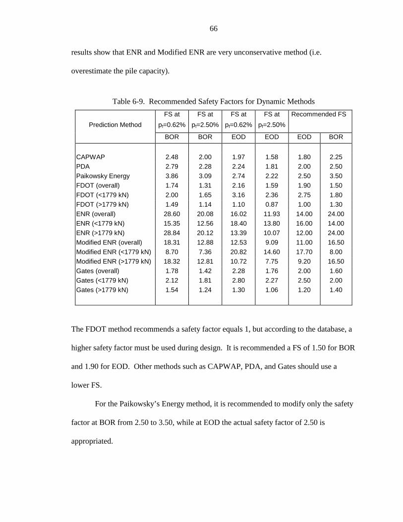
66
results show that ENR and Modified ENR are very unconservative method (i.e.
overestimate the pile capacity).
Table 6-9. Recommended Safety Factors for Dynamic Methods
FS at FS at FS at FS at Recommended FS
Prediction Method pf=0.62% pf=2.50% pf=0.62% pf=2.50%
BOR BOR EOD EOD EOD BOR
CAPWAP 2.48 2.00 1.97 1.58 1.80 2.25
PDA 2.79 2.28 2.24 1.81 2.00 2.50
Paikowsky Energy 3.86 3.09 2.74 2.22 2.50 3.50
FDOT (overall) 1.74 1.31 2.16 1.59 1.90 1.50
FDOT (<1779 kN) 2.00 1.65 3.16 2.36 2.75 1.80
FDOT (>1779 kN) 1.49 1.14 1.10 0.87 1.00 1.30
ENR (overall) 28.60 20.08 16.02 11.93 14.00 24.00
ENR (<1779 kN) 15.35 12.56 18.40 13.80 16.00 14.00
ENR (>1779 kN) 28.84 20.12 13.39 10.07 12.00 24.00
Modified ENR (overall) 18.31 12.88 12.53 9.09 11.00 16.50
Modified ENR (<1779 kN) 8.70 7.36 20.82 14.60 17.70 8.00
Modified ENR (>1779 kN) 18.32 12.81 10.72 7.75 9.20 16.50
Gates (overall) 1.78 1.42 2.28 1.76 2.00 1.60
Gates (<1779 kN) 2.12 1.81 2.80 2.27 2.50 2.00
Gates (>1779 kN) 1.54 1.24 1.30 1.06 1.20 1.40
The FDOT method recommends a safety factor equals 1, but according to the database, a
higher safety factor must be used during design. It is recommended a FS of 1.50 for BOR
and 1.90 for EOD. Other methods such as CAPWAP, PDA, and Gates should use a
lower FS.
For the Paikowsky’s Energy method, it is recommended to modify only the safety
factor at BOR from 2.50 to 3.50, while at EOD the actual safety factor of 2.50 is
appropriated.
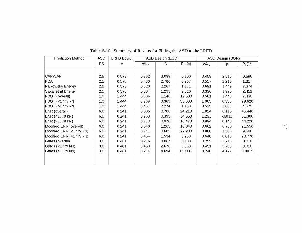
Table 6-10. Summary of Results for Fitting the ASD to the LRFD
Prediction Method ASD LRFD Equiv. ASD Design (EOD) ASD Design (BOR)
FS φ φ/λR β Pf (%) φ/λR β Pf (%)
CAPWAP 2.5 0.578 0.362 3.089 0.100 0.458 2.515 0.596PDA 2.5 0.578 0.430 2.786 0.267 0.557 2.210 1.357Paikowsky Energy 2.5 0.578 0.520 2.267 1.171 0.691 1.449 7.374Sakai et al Energy 2.5 0.578 0.384 1.293 9.810 0.396 1.976 2.411FDOT (overall) 1.0 1.444 0.606 1.146 12.600 0.561 1.445 7.430FDOT (<1779 kN) 1.0 1.444 0.969 0.369 35.630 1.065 0.536 29.620FDOT (>1779 kN) 1.0 1.444 0.457 2.274 1.150 0.525 1.688 4.575ENR (overall) 6.0 0.241 0.805 0.700 24.210 1.024 0.115 45.440ENR (<1779 kN) 6.0 0.241 0.963 0.395 34.660 1.293 -0.032 51.300ENR (>1779 kN) 6.0 0.241 0.713 0.976 16.470 0.994 0.146 44.220Modified ENR (overall) 6.0 0.241 0.540 1.263 10.340 0.662 0.788 21.550Modified ENR (<1779 kN) 6.0 0.241 0.741 0.605 27.280 0.868 1.306 9.586Modified ENR (>1779 kN) 6.0 0.241 0.454 1.534 6.258 0.640 0.815 20.770Gates (overall) 3.0 0.481 0.276 3.067 0.108 0.255 3.718 0.010Gates (<1779 kN) 3.0 0.481 0.450 2.676 0.363 0.451 3.703 0.010Gates (>1779 kN) 3.0 0.481 0.214 4.694 0.0001 0.240 4.177 0.0015
68
ASD Design Evaluation
Because Equation 5-9 relates LRFD to ASD in terms only of the bridge span
length, and load factors, all methods that use the same safety factor will have the same
load resistance factor, φ. These are not the same findings obtained for the reliability
index, β, which depends on the COVR and λR. Table 6-10 presents the LRFD equivalent
load resistance factor, φ, the φ/λR ratio, reliability index, β, and the corresponding
probability of failure, pf (percent) for the actual ASD procedure.
Using as a reference value the AASHTO’s recommended probability of failure for
single piles (i.e. 0.62 % for β = 2.50 and 2.50% for β = 1.96), a comparison of the
probability of failures for each method could be performed. First, the ENR and Modified
ENR procedures show extremely high probability of failures, which reflect the level of
unconservatism as discussed in preceding sections. On the other hand, Gates method
shows a probability of failure as low as 0.010 percent, typical of a very conservative
method. Other methods such as CAPWAP, PDA, and Sakai show relative good
agreement to the recommended probability of failure from AASHTO.
69
CHAPTER 7
SKIN AND TIP STATIC CAPACITY ASSESSMENT OF DRIVEN PILES
As discussed in the previous chapter, the PDA Case method was found to be as
accurate as the other dynamic methods such as Paikowsky and CAPWAP procedures.
This trend was observed for driven piles at both, EOD and BOR.
The PDA Case method results depend on the estimated damping coefficient, Jc.
The recommended values for Jc vary according to the soil type near the tip of the pile. On
the other hand, CAPWAP selects the Coefficient of Damping and the pile resistance in
such a way that the force trace can be reproduced from the velocity trace. The latter
permit CAPWAP to estimate the skin resistance distribution and the tip resistance for any
given pile. The estimate of the skin and tip capacity in addition to the distribution of
damping and skin friction along the pile from CAPWAP have resulted in its use (scour
areas, etc.) versus the PDA, in which only the total static capacity is obtained. However,
CAPWAP is a multi-variable program that requires iterations (i.e. time consuming) and a
significant level of expertise by the technician who use it.
In the next sections, two methods to determine the skin and the tip static capacity
from the PDA traces are presented. The results will be compared to the Davisson’s
capacity determined by the static load test.
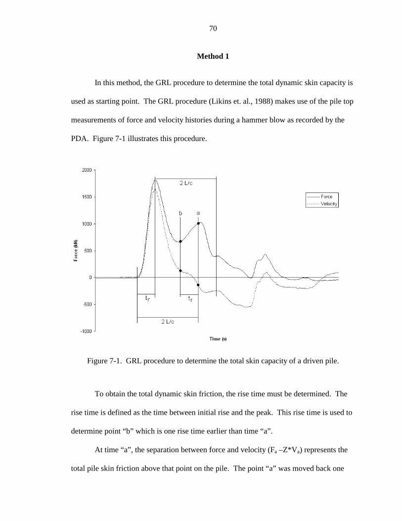
70
Method 1
In this method, the GRL procedure to determine the total dynamic skin capacity is
used as starting point. The GRL procedure (Likins et. al., 1988) makes use of the pile top
measurements of force and velocity histories during a hammer blow as recorded by the
PDA. Figure 7-1 illustrates this procedure.
Figure 7-1. GRL procedure to determine the total skin capacity of a driven pile.
To obtain the total dynamic skin friction, the rise time must be determined. The
rise time is defined as the time between initial rise and the peak. This rise time is used to
determine point “b” which is one rise time earlier than time “a”.
At time “a”, the separation between force and velocity (Fa –Z*Va) represents the
total pile skin friction above that point on the pile. The point “a” was moved back one
71
rise time from 2 L/c to exclude any reflections from the pile tip of the initial input wave.
The assumption of this method is that the skin friction of the bottom one rise length is the
same as the one additional rise time length above. Based on that assumption, the skin
resistance is the separation of force and velocity at point “a” added to the increase in
resistance from point “b” to point “a” as stated below.
( ) ( ) ( )[ ]bbaaaa ZVFZVFZVFSFT −−−+−= (7-1)
Once the estimate of dynamic skin friction is determined using the GRL
procedure, as described above, the static tip and skin capacity were calculated according
to the following methodology (Method 1). First, the total dynamic capacity, RTL, is
determined using the Case solution for dynamic capacity (Equation 3-14 for Jc equals 0).
Then, knowing the total dynamic capacity and the GRL estimate of skin dynamic
capacity, the dynamic tip capacity, TT, could be computed.
SFTRTLTT −= (7-2)
where TT Dynamic Tip Capacity
RTL Total Dynamic Capacity
SFT GRL Estimate of Dynamic Skin Capacity
Then, the total tip to skin capacity ratio, T/S, may be determined
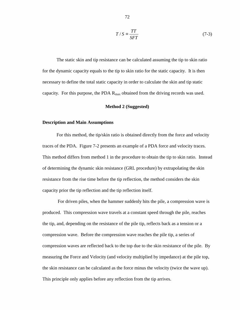
72
SFT
TTST =/ (7-3)
The static skin and tip resistance can be calculated assuming the tip to skin ratio
for the dynamic capacity equals to the tip to skin ratio for the static capacity. It is then
necessary to define the total static capacity in order to calculate the skin and tip static
capacity. For this purpose, the PDA Rmax obtained from the driving records was used.
Method 2 (Suggested)
Description and Main Assumptions
For this method, the tip/skin ratio is obtained directly from the force and velocity
traces of the PDA. Figure 7-2 presents an example of a PDA force and velocity traces.
This method differs from method 1 in the procedure to obtain the tip to skin ratio. Instead
of determining the dynamic skin resistance (GRL procedure) by extrapolating the skin
resistance from the rise time before the tip reflection, the method considers the skin
capacity prior the tip reflection and the tip reflection itself.
For driven piles, when the hammer suddenly hits the pile, a compression wave is
produced. This compression wave travels at a constant speed through the pile, reaches
the tip, and, depending on the resistance of the pile tip, reflects back as a tension or a
compression wave. Before the compression wave reaches the pile tip, a series of
compression waves are reflected back to the top due to the skin resistance of the pile. By
measuring the Force and Velocity (and velocity multiplied by impedance) at the pile top,
the skin resistance can be calculated as the force minus the velocity (twice the wave up).
This principle only applies before any reflection from the tip arrives.
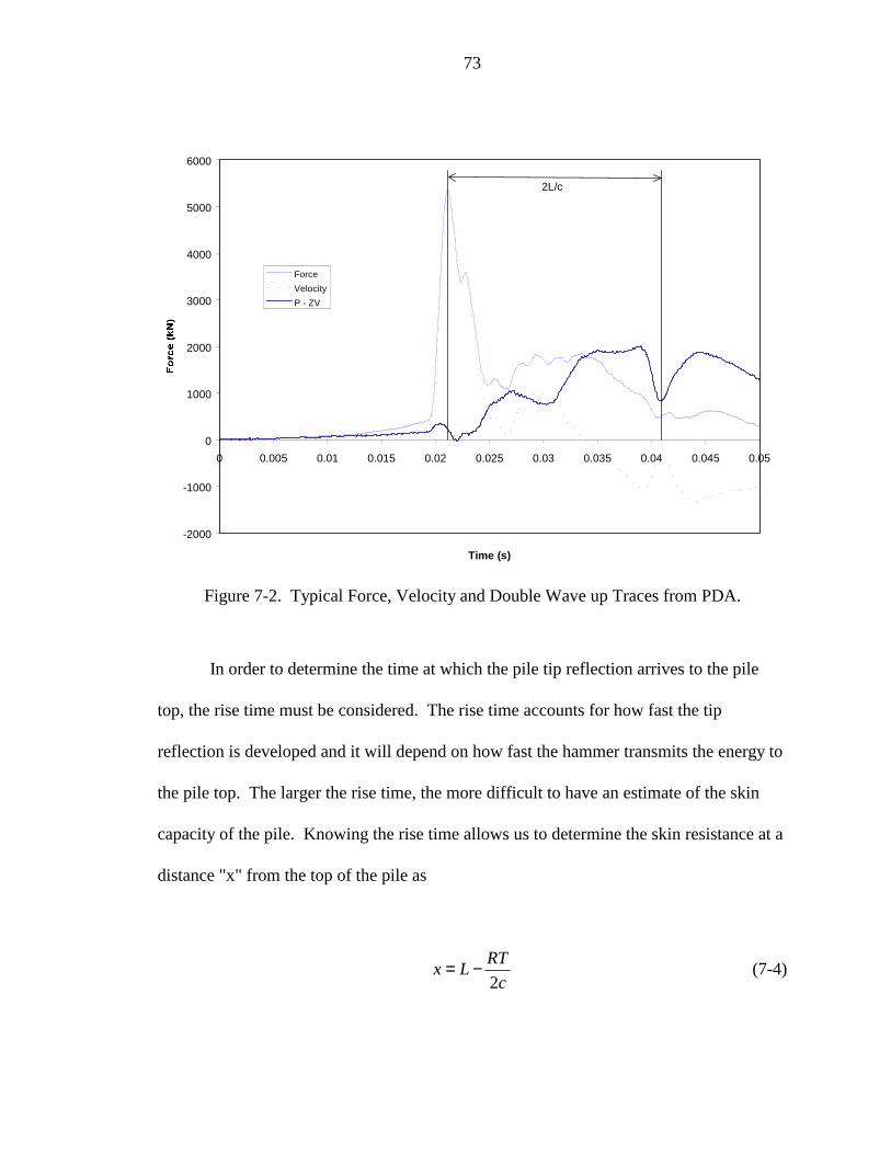
73
-2000
-1000
0
1000
2000
3000
4000
5000
6000
0 0.005 0.01 0.015 0.02 0.025 0.03 0.035 0.04 0.045 0.05
Time (s)
Force
Velocity
P - ZV
2L/c
Figure 7-2. Typical Force, Velocity and Double Wave up Traces from PDA.
In order to determine the time at which the pile tip reflection arrives to the pile
top, the rise time must be considered. The rise time accounts for how fast the tip
reflection is developed and it will depend on how fast the hammer transmits the energy to
the pile top. The larger the rise time, the more difficult to have an estimate of the skin
capacity of the pile. Knowing the rise time allows us to determine the skin resistance at a
distance "x" from the top of the pile as
c
RTLx
2−= (7-4)
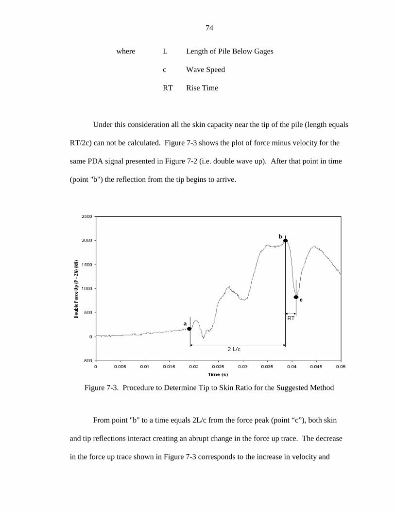
74
where L Length of Pile Below Gages
c Wave Speed
RT Rise Time
Under this consideration all the skin capacity near the tip of the pile (length equals
RT/2c) can not be calculated. Figure 7-3 shows the plot of force minus velocity for the
same PDA signal presented in Figure 7-2 (i.e. double wave up). After that point in time
(point "b") the reflection from the tip begins to arrive.
Figure 7-3. Procedure to Determine Tip to Skin Ratio for the Suggested Method
From point "b" to a time equals 2L/c from the force peak (point “c”), both skin
and tip reflections interact creating an abrupt change in the force up trace. The decrease
in the force up trace shown in Figure 7-3 corresponds to the increase in velocity and
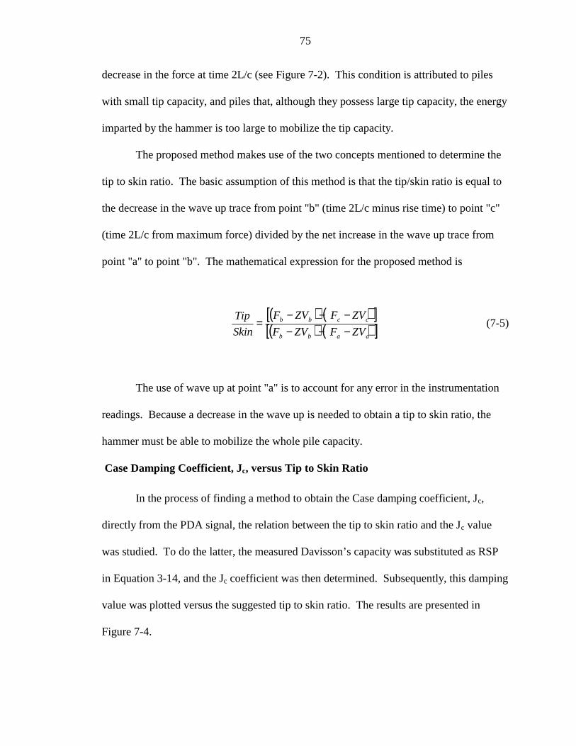
75
decrease in the force at time 2L/c (see Figure 7-2). This condition is attributed to piles
with small tip capacity, and piles that, although they possess large tip capacity, the energy
imparted by the hammer is too large to mobilize the tip capacity.
The proposed method makes use of the two concepts mentioned to determine the
tip to skin ratio. The basic assumption of this method is that the tip/skin ratio is equal to
the decrease in the wave up trace from point "b" (time 2L/c minus rise time) to point "c"
(time 2L/c from maximum force) divided by the net increase in the wave up trace from
point "a" to point "b". The mathematical expression for the proposed method is
( ) ( )[ ]( ) ( )[ ]aabb
ccbb
ZVFZVF
ZVFZVF
Skin
Tip
−−−−−−
= (7-5)
The use of wave up at point "a" is to account for any error in the instrumentation
readings. Because a decrease in the wave up is needed to obtain a tip to skin ratio, the
hammer must be able to mobilize the whole pile capacity.
Case Damping Coefficient, Jc, versus Tip to Skin Ratio
In the process of finding a method to obtain the Case damping coefficient, Jc,
directly from the PDA signal, the relation between the tip to skin ratio and the Jc value
was studied. To do the latter, the measured Davisson’s capacity was substituted as RSP
in Equation 3-14, and the Jc coefficient was then determined. Subsequently, this damping
value was plotted versus the suggested tip to skin ratio. The results are presented in
Figure 7-4.
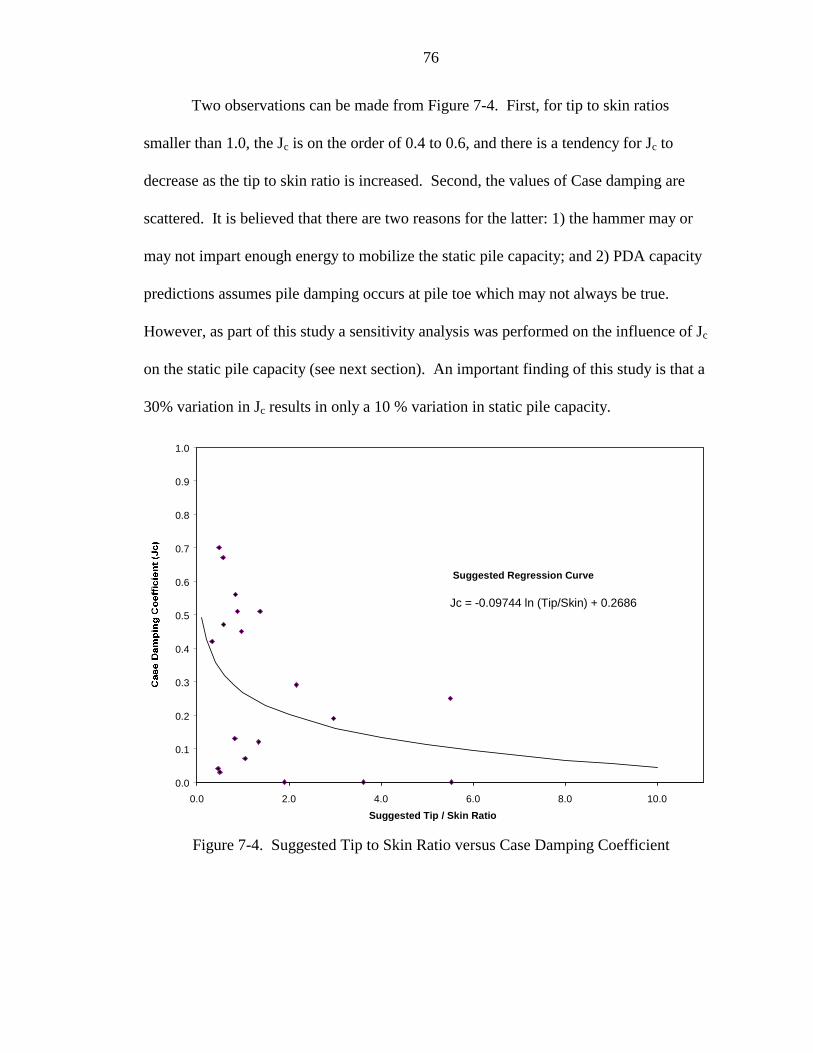
76
Two observations can be made from Figure 7-4. First, for tip to skin ratios
smaller than 1.0, the Jc is on the order of 0.4 to 0.6, and there is a tendency for Jc to
decrease as the tip to skin ratio is increased. Second, the values of Case damping are
scattered. It is believed that there are two reasons for the latter: 1) the hammer may or
may not impart enough energy to mobilize the static pile capacity; and 2) PDA capacity
predictions assumes pile damping occurs at pile toe which may not always be true.
However, as part of this study a sensitivity analysis was performed on the influence of Jc
on the static pile capacity (see next section). An important finding of this study is that a
30% variation in Jc results in only a 10 % variation in static pile capacity.
0.0
0.1
0.2
0.3
0.4
0.5
0.6
0.7
0.8
0.9
1.0
0.0 2.0 4.0 6.0 8.0 10.0
Suggested Tip / Skin Ratio
Suggested Regression Curve
Jc = -0.09744 ln (Tip/Skin) + 0.2686
Figure 7-4. Suggested Tip to Skin Ratio versus Case Damping Coefficient
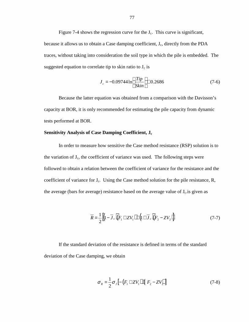
77
Figure 7-4 shows the regression curve for the Jc. This curve is significant,
because it allows us to obtain a Case damping coefficient, Jc, directly from the PDA
traces, without taking into consideration the soil type in which the pile is embedded. The
suggested equation to correlate tip to skin ratio to Jc is
2686.0ln09744.0 +
−=
Skin
TipJc (7-6)
Because the latter equation was obtained from a comparison with the Davisson’s
capacity at BOR, it is only recommended for estimating the pile capacity from dynamic
tests performed at BOR.
Sensitivity Analysis of Case Damping Coefficient, Jc
In order to measure how sensitive the Case method resistance (RSP) solution is to
the variation of Jc, the coefficient of variance was used. The following steps were
followed to obtain a relation between the coefficient of variance for the resistance and the
coefficient of variance for Jc. Using the Case method solution for the pile resistance, R,
the average (bars for average) resistance based on the average value of Jc.is given as
( )( ) ( )( )[ ]2211 112
1ZVFJZVFJR cc −+++−= (7-7)
If the standard deviation of the resistance is defined in terms of the standard
deviation of the Case damping, we obtain
( ) ( )[ ]22112
1ZVFZVFJR −++−= σσ (7-8)
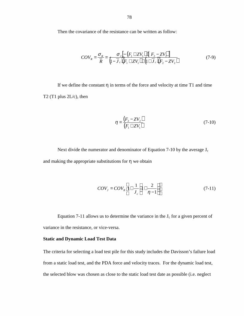
78
Then the covariance of the resistance can be written as follow:
( ) ( )[ ]( )( ) ( )( )2211
2211
11 ZVFJZVFJ
ZVFZVF
RCOV
cc
JRR −+++−
−++−== σσ(7-9)
If we define the constant η in terms of the force and velocity at time T1 and time
T2 (T1 plus 2L/c), then
( )( )11
22
ZVF
ZVF
+−=η (7-10)
Next divide the numerator and denominator of Equation 7-10 by the average Jc
and making the appropriate substitutions for η we obtain
−
++=1
21
11
ηcRJ J
COVCOV (7-11)
Equation 7-11 allows us to determine the variance in the Jc for a given percent of
variance in the resistance, or vice-versa.
Static and Dynamic Load Test Data
The criteria for selecting a load test pile for this study includes the Davisson’s failure load
from a static load test, and the PDA force and velocity traces. For the dynamic load test,
the selected blow was chosen as close to the static load test date as possible (i.e. neglect
79
freeze). For all the cases, the dynamic load test closer to the static load test was
performed after the load test (i.e. the static capacity was compared to the Beginning of
Restrike). Other requirements include having a measured skin capacity by mean of a pull
out static load test or Osterberg load cell test. For each pile, it was required to know both
geometric and driving parameters, such as, wave speed, pile length below the gages,
cross-sectional area, and material modulus. Based on the latter requirements, 18 test pile
were considered. Table 7-1 summarizes general information of each load test pile. The
pile population represents 9 sites and 3 diameters, while the range of depths of the piles
below the gages varies from 9.15 to 34.45 meters. Only one test pile is from a location
outside the State of Florida.
Automating the Suggested Method
A Fortran program was developed in order to simplify the calculation process.
This program is able to read directly from the PDA record the force and velocity signal
and perform the data reduction. The input parameters for this program are the length of
the pile below the gages, the wave speed, the material modulus, the cross-sectional area,
and the data-sampling interval.
The output file contains a general description of the pile itself and the driving
information entered previously. In addition, it presents in a tabular form the time
increment, velocity, force, velocity times impedance, displacement, and double wave up
(P – ZV). The latter information can be easily plotted to obtain the PDA traces.
Appendix I contains the PDA traces (force, velocity, double force up, and displacement)
for the signals studied. At the end of the output file, the results from the suggested
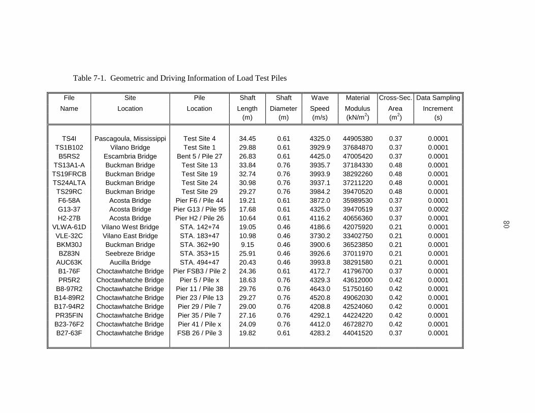
Table 7-1. Geometric and Driving Information of Load Test Piles
File Site Pile Shaft Shaft Wave Material Cross-Sec. Data Sampling
Name Location Location Length Diameter Speed Modulus Area Increment(m) (m) (m/s) (kN/m2) (m2) (s)
TS4I Pascagoula, Mississippi Test Site 4 34.45 0.61 4325.0 44905380 0.37 0.0001TS1B102 Vilano Bridge Test Site 1 29.88 0.61 3929.9 37684870 0.37 0.0001B5RS2 Escambria Bridge Bent 5 / Pile 27 26.83 0.61 4425.0 47005420 0.37 0.0001
TS13A1-A Buckman Bridge Test Site 13 33.84 0.76 3935.7 37184330 0.48 0.0001TS19FRCB Buckman Bridge Test Site 19 32.74 0.76 3993.9 38292260 0.48 0.0001TS24ALTA Buckman Bridge Test Site 24 30.98 0.76 3937.1 37211220 0.48 0.0001TS29RC Buckman Bridge Test Site 29 29.27 0.76 3984.2 39470520 0.48 0.0001F6-58A Acosta Bridge Pier F6 / Pile 44 19.21 0.61 3872.0 35989530 0.37 0.0001G13-37 Acosta Bridge Pier G13 / Pile 95 17.68 0.61 4325.0 39470519 0.37 0.0002H2-27B Acosta Bridge Pier H2 / Pile 26 10.64 0.61 4116.2 40656360 0.37 0.0001
VLWA-61D Vilano West Bridge STA. 142+74 19.05 0.46 4186.6 42075920 0.21 0.0001VLE-32C Vilano East Bridge STA. 183+47 10.98 0.46 3730.2 33402750 0.21 0.0001BKM30J Buckman Bridge STA. 362+90 9.15 0.46 3900.6 36523850 0.21 0.0001BZ83N Seebreze Bridge STA. 353+15 25.91 0.46 3926.6 37011970 0.21 0.0001
AUC63K Aucilla Bridge STA. 494+47 20.43 0.46 3993.8 38291580 0.21 0.0001B1-76F Choctawhatche Bridge Pier FSB3 / Pile 2 24.36 0.61 4172.7 41796700 0.37 0.0001PR5R2 Choctawhatche Bridge Pier 5 / Pile x 18.63 0.76 4329.3 43612000 0.42 0.0001
B8-97R2 Choctawhatche Bridge Pier 11 / Pile 38 29.76 0.76 4643.0 51750160 0.42 0.0001B14-89R2 Choctawhatche Bridge Pier 23 / Pile 13 29.27 0.76 4520.8 49062030 0.42 0.0001B17-94R2 Choctawhatche Bridge Pier 29 / Pile 7 29.00 0.76 4208.8 42524060 0.42 0.0001PR35FIN Choctawhatche Bridge Pier 35 / Pile 7 27.16 0.76 4292.1 44224220 0.42 0.0001B23-76F2 Choctawhatche Bridge Pier 41 / Pile x 24.09 0.76 4412.0 46728270 0.42 0.0001B27-63F Choctawhatche Bridge FSB 26 / Pile 3 19.82 0.61 4283.2 44041520 0.37 0.0001
81
method and the GRL procedure are presented. In addition, the important time records
such as the time of maximum force, T1, and time T2 (T1 + 2L/c), rise time, etc, are also
presented. Appendix J presents an example of the Fortran output. Only the first five
pages and the last page of the output are included.
Results and Analysis
In the following sections, the results from the suggested method will be presented
in addition to the results of other methodologies such as method 1, PDA, and the
CAPWAP procedure. The reader is referred to Appendix I for the plots of force, velocity,
double wave up, and displacement traces for each case studied. In order to evaluate the
accuracy of the methods studied, a series of comparison of total static capacity have been
performed in relation to the static load capacity. In addition, the predicted skin capacity
of the piles was evaluated for piles with performed pullout tests or Osterberg tests in
which skin failure occurred.
Presentation of Results
Table 7-2 summarizes the results for the suggested method and the load tests. The
tip to skin ratio is presented together with the recommended Case damping coefficient, Jc.
Based on these two parameters and using the PDA Case solution, the total capacity was
computed.
The load test results include the Davisson’s capacity for all compression tests and
the skin capacity for piles with a performed tensile load test or an Osterberg test with skin
failure. Table 7-3 presents the estimated capacities using Method 1 and CAPWAP.
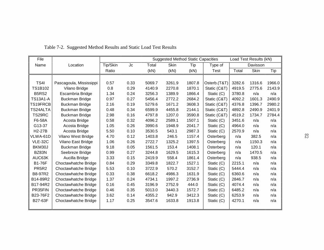
Table 7-2. Suggested Method Results and Static Load Test Results
File Suggested Method Static Capacities Load Test Results (kN)
Name Location Tip/Skin Jc Total Skin Tip Type of DavissonRatio (kN) (kN) (kN) Test Total Skin Tip
TS4I Pascagoula, Mississippi 0.57 0.33 5069.7 3261.9 1807.8 Osterb.(T&T) 3282.6 1316.6 1966.0TS1B102 Vilano Bridge 0.8 0.29 4140.9 2270.8 1870.1 Static (C&T) 4919.5 2775.6 2143.9B5RS2 Escambria Bridge 1.34 0.24 3256.3 1389.9 1866.4 Static (C) 3780.8 n/a n/a
TS13A1-A Buckman Bridge 0.97 0.27 5456.4 2772.2 2684.2 Static (C&T) 4092.2 1601.3 2490.9TS19FRCB Buckman Bridge 2.16 0.19 5279.6 1671.2 3608.3 Static (C&T) 4376.8 1396.7 2980.2TS24ALTA Buckman Bridge 0.48 0.34 6599.9 4455.8 2144.1 Static (C&T) 4892.8 2490.9 2401.9TS29RC Buckman Bridge 2.98 0.16 4797.8 1207.0 3590.8 Static (C&T) 4519.2 1734.7 2784.4F6-58A Acosta Bridge 0.58 0.32 4096.2 2589.1 1507.1 Static (C) 3451.6 n/a n/aG13-37 Acosta Bridge 1.05 0.26 3990.6 1948.9 2041.7 Static (C) 4964.0 n/a n/aH2-27B Acosta Bridge 5.50 0.10 3530.5 543.1 2987.3 Static (C) 2570.9 n/a n/a
VLWA-61D Vilano West Bridge 4.70 0.12 1403.8 246.5 1157.4 Osterberg n/a 382.5 n/aVLE-32C Vilano East Bridge 1.06 0.26 2722.7 1325.2 1397.5 Osterberg n/a 1150.3 n/aBKM30J Buckman Bridge 9.18 0.05 1561.5 153.4 1408.1 Osterberg n/a 120.1 n/aBZ83N Seebreze Bridge 0.99 0.27 3244.8 1629.5 1615.3 Osterberg n/a 1470.5 n/a
AUC63K Aucilla Bridge 3.33 0.15 2419.9 558.4 1861.4 Osterberg n/a 938.5 n/aB1-76F Choctawhatche Bridge 0.84 0.29 3349.8 1822.7 1527.1 Static (C) 2215.1 n/a n/aPR5R2 Choctawhatche Bridge 5.53 0.10 3722.9 570.2 3152.7 Static (C) 5444.4 n/a n/a
B8-97R2 Choctawhatche Bridge 0.33 0.38 6618.2 4986.3 1631.9 Static (C) 6360.6 n/a n/aB14-89R2 Choctawhatche Bridge 1.37 0.24 4734.1 1997.2 2736.9 Static (C) 2846.7 n/a n/aB17-94R2 Choctawhatche Bridge 0.16 0.45 3196.9 2752.9 444.0 Static (C) 4074.4 n/a n/aPR35FIN Choctawhatche Bridge 0.46 0.35 5013.0 3440.3 1572.7 Static (C) 6485.2 n/a n/aB23-76F2 Choctawhatche Bridge 3.62 0.14 4355.2 942.9 3412.3 Static (C) 6253.9 n/a n/aB27-63F Choctawhatche Bridge 1.17 0.25 3547.6 1633.8 1913.8 Static (C) 4270.1 n/a n/a
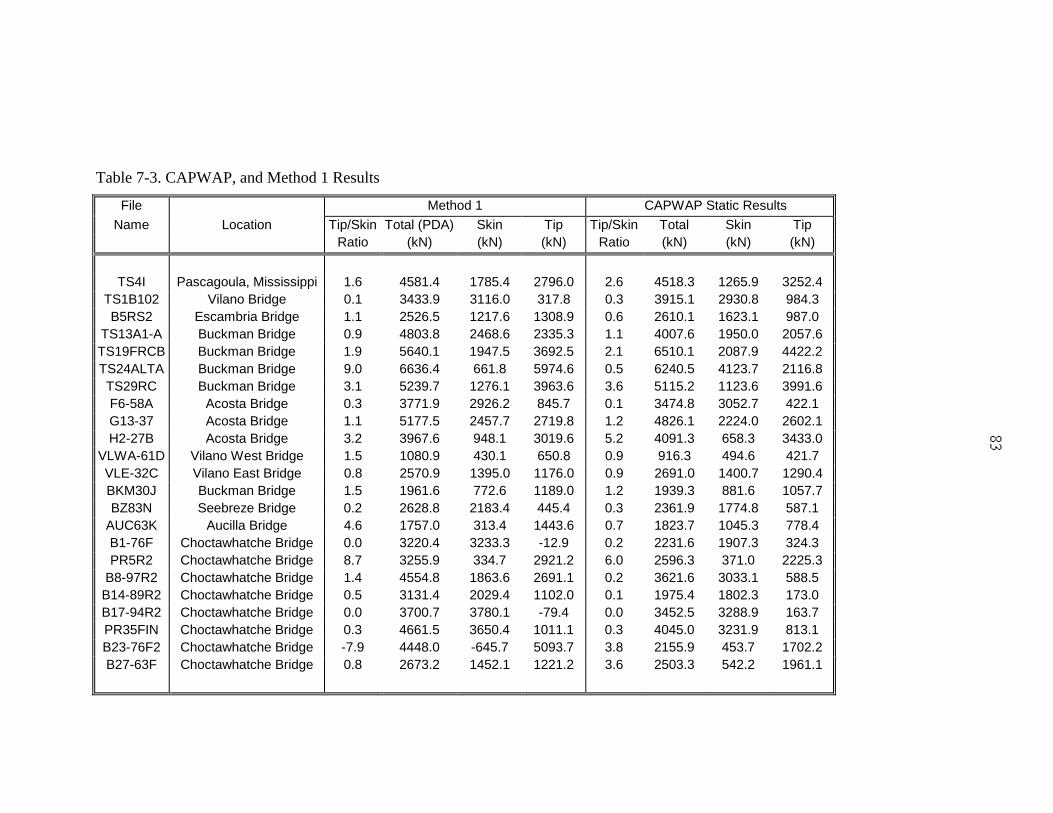
Table 7-3. CAPWAP, and Method 1 Results
File Method 1 CAPWAP Static Results
Name Location Tip/Skin Total (PDA) Skin Tip Tip/Skin Total Skin TipRatio (kN) (kN) (kN) Ratio (kN) (kN) (kN)
TS4I Pascagoula, Mississippi 1.6 4581.4 1785.4 2796.0 2.6 4518.3 1265.9 3252.4TS1B102 Vilano Bridge 0.1 3433.9 3116.0 317.8 0.3 3915.1 2930.8 984.3B5RS2 Escambria Bridge 1.1 2526.5 1217.6 1308.9 0.6 2610.1 1623.1 987.0
TS13A1-A Buckman Bridge 0.9 4803.8 2468.6 2335.3 1.1 4007.6 1950.0 2057.6TS19FRCB Buckman Bridge 1.9 5640.1 1947.5 3692.5 2.1 6510.1 2087.9 4422.2TS24ALTA Buckman Bridge 9.0 6636.4 661.8 5974.6 0.5 6240.5 4123.7 2116.8TS29RC Buckman Bridge 3.1 5239.7 1276.1 3963.6 3.6 5115.2 1123.6 3991.6F6-58A Acosta Bridge 0.3 3771.9 2926.2 845.7 0.1 3474.8 3052.7 422.1G13-37 Acosta Bridge 1.1 5177.5 2457.7 2719.8 1.2 4826.1 2224.0 2602.1H2-27B Acosta Bridge 3.2 3967.6 948.1 3019.6 5.2 4091.3 658.3 3433.0
VLWA-61D Vilano West Bridge 1.5 1080.9 430.1 650.8 0.9 916.3 494.6 421.7VLE-32C Vilano East Bridge 0.8 2570.9 1395.0 1176.0 0.9 2691.0 1400.7 1290.4BKM30J Buckman Bridge 1.5 1961.6 772.6 1189.0 1.2 1939.3 881.6 1057.7BZ83N Seebreze Bridge 0.2 2628.8 2183.4 445.4 0.3 2361.9 1774.8 587.1
AUC63K Aucilla Bridge 4.6 1757.0 313.4 1443.6 0.7 1823.7 1045.3 778.4B1-76F Choctawhatche Bridge 0.0 3220.4 3233.3 -12.9 0.2 2231.6 1907.3 324.3PR5R2 Choctawhatche Bridge 8.7 3255.9 334.7 2921.2 6.0 2596.3 371.0 2225.3
B8-97R2 Choctawhatche Bridge 1.4 4554.8 1863.6 2691.1 0.2 3621.6 3033.1 588.5B14-89R2 Choctawhatche Bridge 0.5 3131.4 2029.4 1102.0 0.1 1975.4 1802.3 173.0B17-94R2 Choctawhatche Bridge 0.0 3700.7 3780.1 -79.4 0.0 3452.5 3288.9 163.7PR35FIN Choctawhatche Bridge 0.3 4661.5 3650.4 1011.1 0.3 4045.0 3231.9 813.1B23-76F2 Choctawhatche Bridge -7.9 4448.0 -645.7 5093.7 3.8 2155.9 453.7 1702.2B27-63F Choctawhatche Bridge 0.8 2673.2 1452.1 1221.2 3.6 2503.3 542.2 1961.1
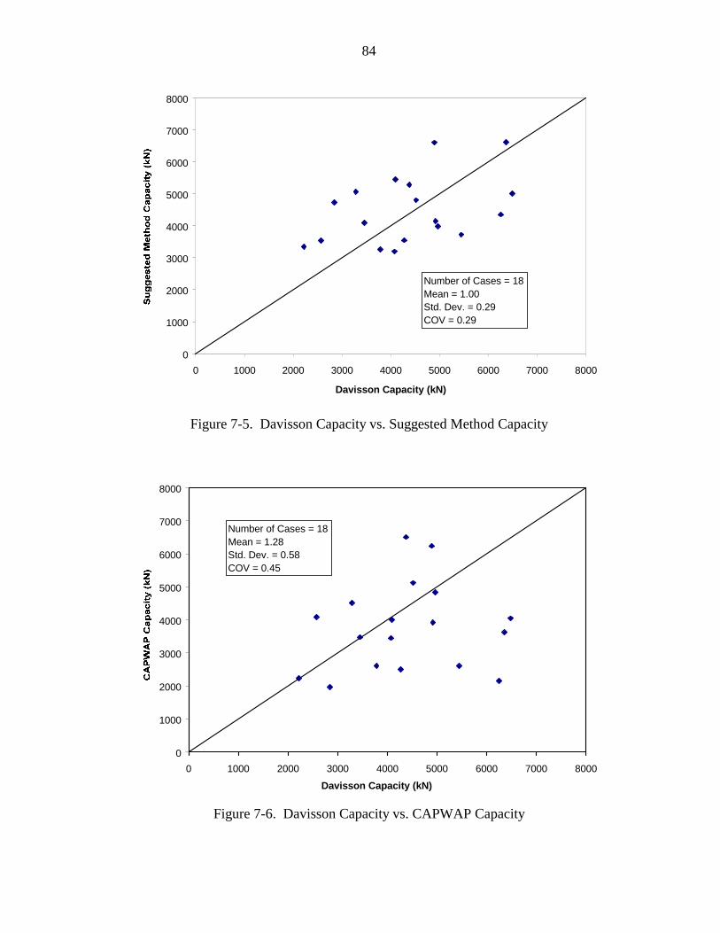
84
0
1000
2000
3000
4000
5000
6000
7000
8000
0 1000 2000 3000 4000 5000 6000 7000 8000
Davisson Capacity (kN)
Number of Cases = 18Mean = 1.00Std. Dev. = 0.29COV = 0.29
Figure 7-5. Davisson Capacity vs. Suggested Method Capacity
0
1000
2000
3000
4000
5000
6000
7000
8000
0 1000 2000 3000 4000 5000 6000 7000 8000
Davisson Capacity (kN)
Number of Cases = 18Mean = 1.28Std. Dev. = 0.58COV = 0.45
Figure 7-6. Davisson Capacity vs. CAPWAP Capacity
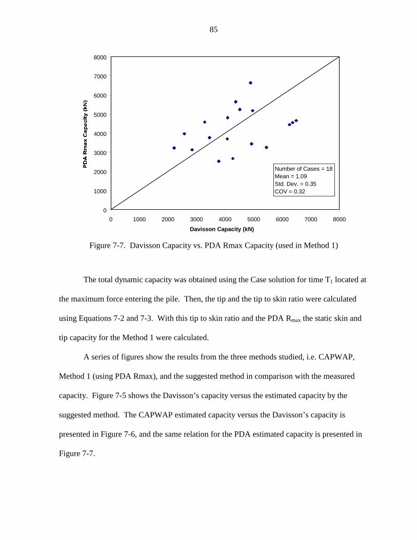
85
0
1000
2000
3000
4000
5000
6000
7000
8000
0 1000 2000 3000 4000 5000 6000 7000 8000
Davisson Capacity (kN)
Number of Cases = 18Mean = 1.09Std. Dev. = 0.35COV = 0.32
Figure 7-7. Davisson Capacity vs. PDA Rmax Capacity (used in Method 1)
The total dynamic capacity was obtained using the Case solution for time T1 located at
the maximum force entering the pile. Then, the tip and the tip to skin ratio were calculated
using Equations 7-2 and 7-3. With this tip to skin ratio and the PDA Rmax the static skin and
tip capacity for the Method 1 were calculated.
A series of figures show the results from the three methods studied, i.e. CAPWAP,
Method 1 (using PDA Rmax), and the suggested method in comparison with the measured
capacity. Figure 7-5 shows the Davisson’s capacity versus the estimated capacity by the
suggested method. The CAPWAP estimated capacity versus the Davisson’s capacity is
presented in Figure 7-6, and the same relation for the PDA estimated capacity is presented in
Figure 7-7.
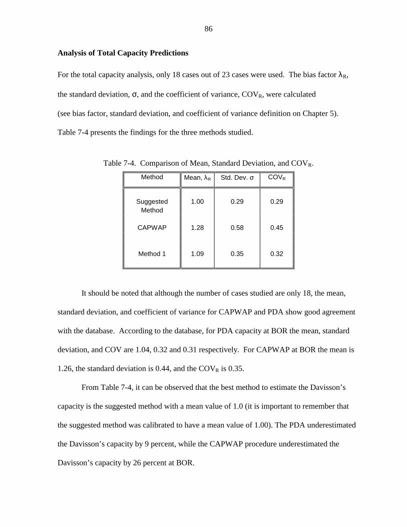
86
Analysis of Total Capacity Predictions
For the total capacity analysis, only 18 cases out of 23 cases were used. The bias factor λR,
the standard deviation, σ, and the coefficient of variance, COVR, were calculated
(see bias factor, standard deviation, and coefficient of variance definition on Chapter 5).
Table 7-4 presents the findings for the three methods studied.
Table 7-4. Comparison of Mean, Standard Deviation, and COVR.
Method Mean, λR Std. Dev. σ COVR
Suggested 1.00 0.29 0.29Method
CAPWAP 1.28 0.58 0.45
Method 1 1.09 0.35 0.32
It should be noted that although the number of cases studied are only 18, the mean,
standard deviation, and coefficient of variance for CAPWAP and PDA show good agreement
with the database. According to the database, for PDA capacity at BOR the mean, standard
deviation, and COV are 1.04, 0.32 and 0.31 respectively. For CAPWAP at BOR the mean is
1.26, the standard deviation is 0.44, and the COVR is 0.35.
From Table 7-4, it can be observed that the best method to estimate the Davisson’s
capacity is the suggested method with a mean value of 1.0 (it is important to remember that
the suggested method was calibrated to have a mean value of 1.00). The PDA underestimated
the Davisson’s capacity by 9 percent, while the CAPWAP procedure underestimated the
Davisson’s capacity by 26 percent at BOR.
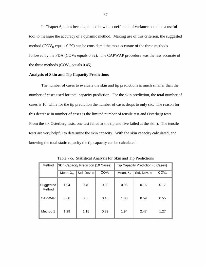
87
In Chapter 6, it has been explained how the coefficient of variance could be a useful
tool to measure the accuracy of a dynamic method. Making use of this criterion, the suggested
method (COVR equals 0.29) can be considered the most accurate of the three methods
followed by the PDA (COVR equals 0.32). The CAPWAP procedure was the less accurate of
the three methods (COVR equals 0.45).
Analysis of Skin and Tip Capacity Predictions
The number of cases to evaluate the skin and tip predictions is much smaller than the
number of cases used for total capacity prediction. For the skin prediction, the total number of
cases is 10, while for the tip prediction the number of cases drops to only six. The reason for
this decrease in number of cases is the limited number of tensile test and Osterberg tests.
From the six Osterberg tests, one test failed at the tip and five failed at the skin). The tensile
tests are very helpful to determine the skin capacity. With the skin capacity calculated, and
knowing the total static capacity the tip capacity can be calculated.
Table 7-5. Statistical Analysis for Skin and Tip Predictions
Method Skin Capacity Prediction (10 Cases) Tip Capacity Prediction (6 Cases)
Mean, λR Std. Dev. σ COVR Mean, λR Std. Dev. σ COVR
Suggested 1.04 0.40 0.39 0.96 0.16 0.17Method
CAPWAP 0.80 0.35 0.43 1.08 0.59 0.55
Method 1 1.29 1.15 0.89 1.94 2.47 1.27
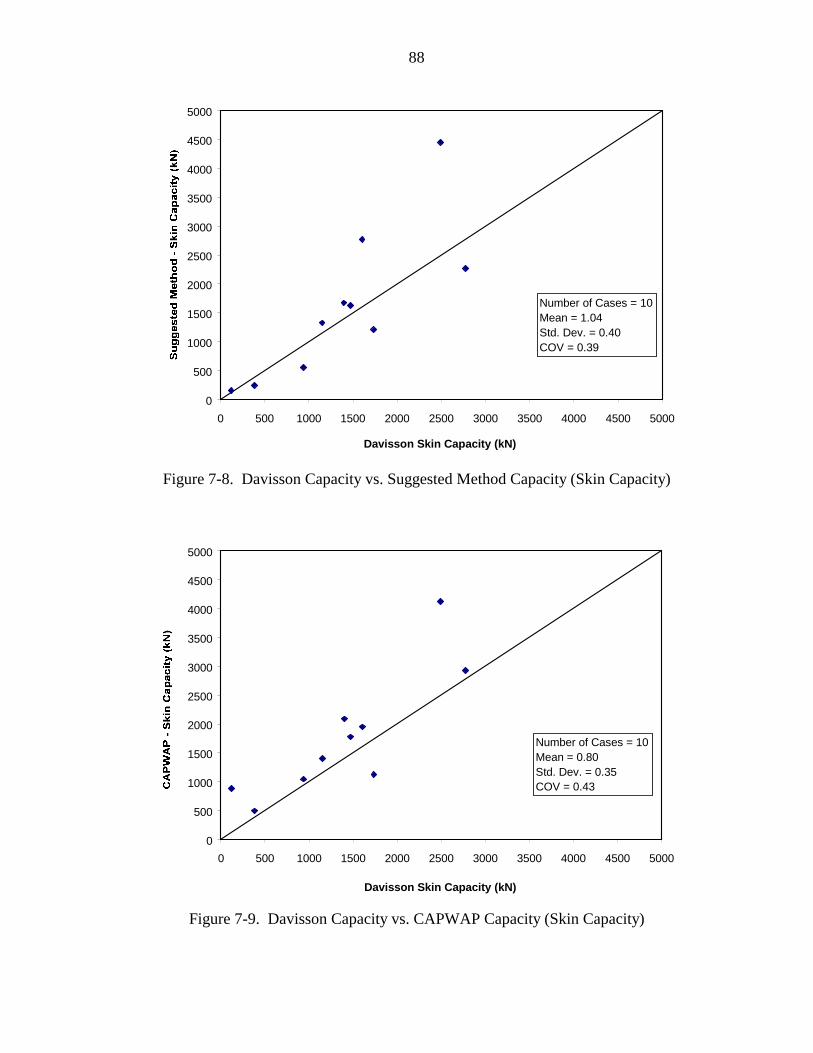
88
0
500
1000
1500
2000
2500
3000
3500
4000
4500
5000
0 500 1000 1500 2000 2500 3000 3500 4000 4500 5000
Davisson Skin Capacity (kN)
Number of Cases = 10Mean = 1.04Std. Dev. = 0.40COV = 0.39
Figure 7-8. Davisson Capacity vs. Suggested Method Capacity (Skin Capacity)
0
500
1000
1500
2000
2500
3000
3500
4000
4500
5000
0 500 1000 1500 2000 2500 3000 3500 4000 4500 5000
Davisson Skin Capacity (kN)
Number of Cases = 10Mean = 0.80Std. Dev. = 0.35COV = 0.43
Figure 7-9. Davisson Capacity vs. CAPWAP Capacity (Skin Capacity)
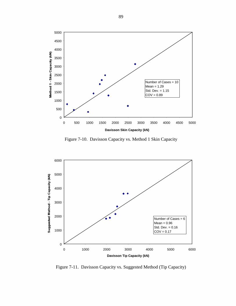
89
0
500
1000
1500
2000
2500
3000
3500
4000
4500
5000
0 500 1000 1500 2000 2500 3000 3500 4000 4500 5000
Davisson Skin Capacity (kN)
Number of Cases = 10Mean = 1.29Std. Dev. = 1.15COV = 0.89
Figure 7-10. Davisson Capacity vs. Method 1 Skin Capacity
0
1000
2000
3000
4000
5000
6000
0 1000 2000 3000 4000 5000 6000
Davisson Tip Capacity (kN)
Number of Cases = 6Mean = 0.96Std. Dev. = 0.16COV = 0.17
Figure 7-11. Davisson Capacity vs. Suggested Method (Tip Capacity)
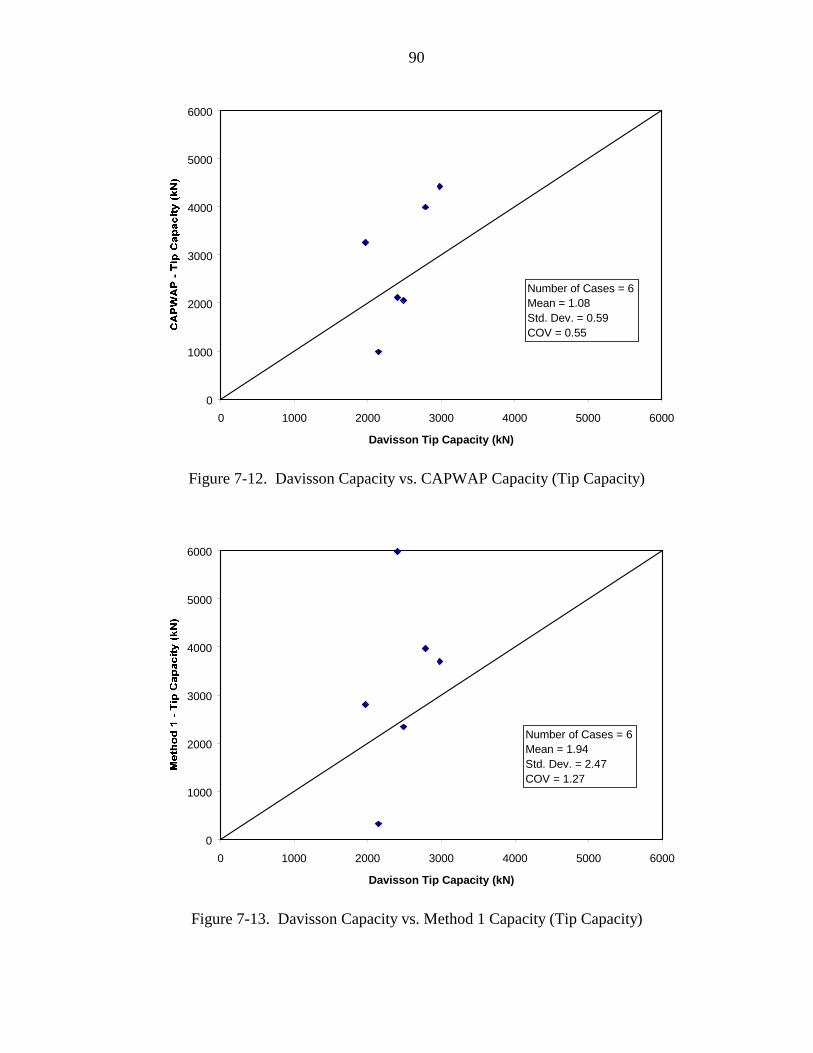
90
0
1000
2000
3000
4000
5000
6000
0 1000 2000 3000 4000 5000 6000
Davisson Tip Capacity (kN)
Number of Cases = 6Mean = 1.08Std. Dev. = 0.59COV = 0.55
Figure 7-12. Davisson Capacity vs. CAPWAP Capacity (Tip Capacity)
0
1000
2000
3000
4000
5000
6000
0 1000 2000 3000 4000 5000 6000
Davisson Tip Capacity (kN)
Number of Cases = 6Mean = 1.94Std. Dev. = 2.47COV = 1.27
Figure 7-13. Davisson Capacity vs. Method 1 Capacity (Tip Capacity)
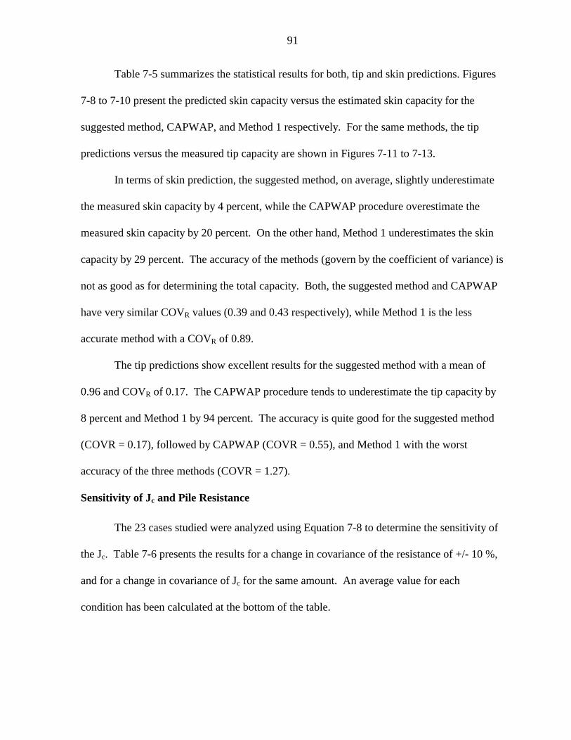
91
Table 7-5 summarizes the statistical results for both, tip and skin predictions. Figures
7-8 to 7-10 present the predicted skin capacity versus the estimated skin capacity for the
suggested method, CAPWAP, and Method 1 respectively. For the same methods, the tip
predictions versus the measured tip capacity are shown in Figures 7-11 to 7-13.
In terms of skin prediction, the suggested method, on average, slightly underestimate
the measured skin capacity by 4 percent, while the CAPWAP procedure overestimate the
measured skin capacity by 20 percent. On the other hand, Method 1 underestimates the skin
capacity by 29 percent. The accuracy of the methods (govern by the coefficient of variance) is
not as good as for determining the total capacity. Both, the suggested method and CAPWAP
have very similar COVR values (0.39 and 0.43 respectively), while Method 1 is the less
accurate method with a COVR of 0.89.
The tip predictions show excellent results for the suggested method with a mean of
0.96 and COVR of 0.17. The CAPWAP procedure tends to underestimate the tip capacity by
8 percent and Method 1 by 94 percent. The accuracy is quite good for the suggested method
(COVR = 0.17), followed by CAPWAP (COVR = 0.55), and Method 1 with the worst
accuracy of the three methods (COVR = 1.27).
Sensitivity of Jc and Pile Resistance
The 23 cases studied were analyzed using Equation 7-8 to determine the sensitivity of
the Jc. Table 7-6 presents the results for a change in covariance of the resistance of +/- 10 %,
and for a change in covariance of Jc for the same amount. An average value for each
condition has been calculated at the bottom of the table.
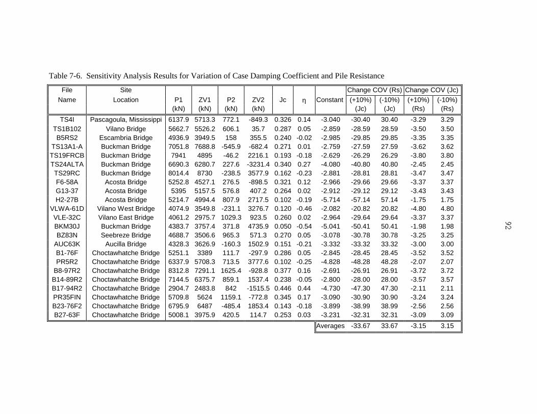
Table 7-6. Sensitivity Analysis Results for Variation of Case Damping Coefficient and Pile Resistance
File Site Change COV (Rs) Change COV (Jc)
Name Location P1 ZV1 P2 ZV2 Jc η Constant (+10%) (-10%) (+10%) (-10%)(kN) (kN) (kN) (kN) (Jc) (Jc) (Rs) (Rs)
TS4I Pascagoula, Mississippi 6137.9 5713.3 772.1 -849.3 0.326 0.14 -3.040 -30.40 30.40 -3.29 3.29TS1B102 Vilano Bridge 5662.7 5526.2 606.1 35.7 0.287 0.05 -2.859 -28.59 28.59 -3.50 3.50B5RS2 Escambria Bridge 4936.9 3949.5 158 355.5 0.240 -0.02 -2.985 -29.85 29.85 -3.35 3.35
TS13A1-A Buckman Bridge 7051.8 7688.8 -545.9 -682.4 0.271 0.01 -2.759 -27.59 27.59 -3.62 3.62TS19FRCB Buckman Bridge 7941 4895 -46.2 2216.1 0.193 -0.18 -2.629 -26.29 26.29 -3.80 3.80TS24ALTA Buckman Bridge 6690.3 6280.7 227.6 -3231.4 0.340 0.27 -4.080 -40.80 40.80 -2.45 2.45TS29RC Buckman Bridge 8014.4 8730 -238.5 3577.9 0.162 -0.23 -2.881 -28.81 28.81 -3.47 3.47F6-58A Acosta Bridge 5252.8 4527.1 276.5 -898.5 0.321 0.12 -2.966 -29.66 29.66 -3.37 3.37G13-37 Acosta Bridge 5395 5157.5 576.8 407.2 0.264 0.02 -2.912 -29.12 29.12 -3.43 3.43H2-27B Acosta Bridge 5214.7 4994.4 807.9 2717.5 0.102 -0.19 -5.714 -57.14 57.14 -1.75 1.75
VLWA-61D Vilano West Bridge 4074.9 3549.8 -231.1 3276.7 0.120 -0.46 -2.082 -20.82 20.82 -4.80 4.80VLE-32C Vilano East Bridge 4061.2 2975.7 1029.3 923.5 0.260 0.02 -2.964 -29.64 29.64 -3.37 3.37BKM30J Buckman Bridge 4383.7 3757.4 371.8 4735.9 0.050 -0.54 -5.041 -50.41 50.41 -1.98 1.98BZ83N Seebreze Bridge 4688.7 3506.6 965.3 571.3 0.270 0.05 -3.078 -30.78 30.78 -3.25 3.25
AUC63K Aucilla Bridge 4328.3 3626.9 -160.3 1502.9 0.151 -0.21 -3.332 -33.32 33.32 -3.00 3.00B1-76F Choctawhatche Bridge 5251.1 3389 111.7 -297.9 0.286 0.05 -2.845 -28.45 28.45 -3.52 3.52PR5R2 Choctawhatche Bridge 6337.9 5708.3 713.5 3777.6 0.102 -0.25 -4.828 -48.28 48.28 -2.07 2.07
B8-97R2 Choctawhatche Bridge 8312.8 7291.1 1625.4 -928.8 0.377 0.16 -2.691 -26.91 26.91 -3.72 3.72B14-89R2 Choctawhatche Bridge 7144.5 6375.7 859.1 1537.4 0.238 -0.05 -2.800 -28.00 28.00 -3.57 3.57B17-94R2 Choctawhatche Bridge 2904.7 2483.8 842 -1515.5 0.446 0.44 -4.730 -47.30 47.30 -2.11 2.11PR35FIN Choctawhatche Bridge 5709.8 5624 1159.1 -772.8 0.345 0.17 -3.090 -30.90 30.90 -3.24 3.24B23-76F2 Choctawhatche Bridge 6795.9 6487 -485.4 1853.4 0.143 -0.18 -3.899 -38.99 38.99 -2.56 2.56B27-63F Choctawhatche Bridge 5008.1 3975.9 420.5 114.7 0.253 0.03 -3.231 -32.31 32.31 -3.09 3.09
Averages -33.67 33.67 -3.15 3.15
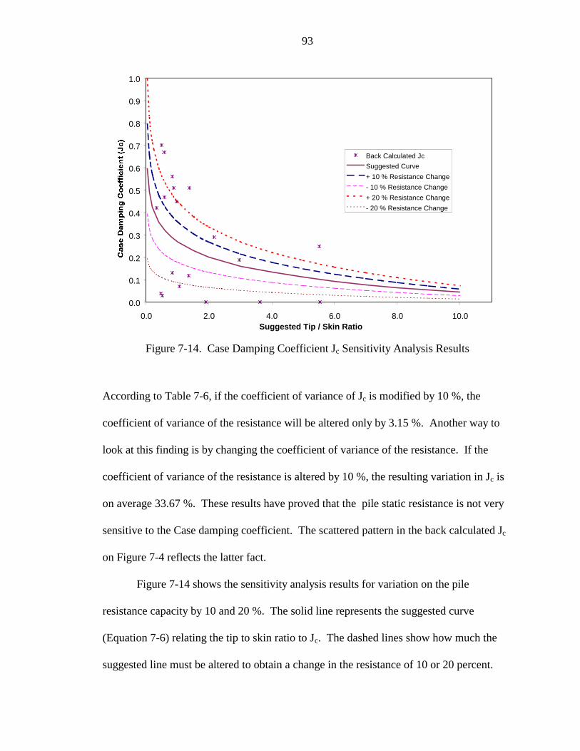
93
0.0
0.1
0.2
0.3
0.4
0.5
0.6
0.7
0.8
0.9
1.0
0.0 2.0 4.0 6.0 8.0 10.0Suggested Tip / Skin Ratio
Back Calculated Jc
Suggested Curve
+ 10 % Resistance Change
- 10 % Resistance Change
+ 20 % Resistance Change
- 20 % Resistance Change
Figure 7-14. Case Damping Coefficient Jc Sensitivity Analysis Results
According to Table 7-6, if the coefficient of variance of Jc is modified by 10 %, the
coefficient of variance of the resistance will be altered only by 3.15 %. Another way to
look at this finding is by changing the coefficient of variance of the resistance. If the
coefficient of variance of the resistance is altered by 10 %, the resulting variation in Jc is
on average 33.67 %. These results have proved that the pile static resistance is not very
sensitive to the Case damping coefficient. The scattered pattern in the back calculated Jc
on Figure 7-4 reflects the latter fact.
Figure 7-14 shows the sensitivity analysis results for variation on the pile
resistance capacity by 10 and 20 %. The solid line represents the suggested curve
(Equation 7-6) relating the tip to skin ratio to Jc. The dashed lines show how much the
suggested line must be altered to obtain a change in the resistance of 10 or 20 percent.
94
CHAPTER 8
CONCLUSIONS AND RECOMMENDATIONS
The conclusions and recommendations presented in this chapter are subdivided
into two sections. The LRFD study conclusions and recommendations are presented first,
followed by those to determine the PDA Case damping coefficient, Jc, and tip/skin ratio
for static pile resistance from the PDA trace.
LRFD Calibration for Eight Dynamic Methods
Conclusions
Eight dynamic methods were evaluated based on a Florida database and LRFD
design procedures. The following conclusions can be drawn from this study:
1. The bridge span length has negligible effect on the resistance factor, φ, or the
corresponding safety factor.
2. The accuracy and efficiency of dynamic methods should be evaluated by their
COVR or φ/λR values, rather than their absolute values of the φ factor.
3. The accuracy (COVR & φ/λR) of dynamic methods from testing at BOR show
negligible increase over the same testing at EOD.
4. The evaluation of φ/λR shows that the new dynamic methods are more cost
effective to meet a reliability index in comparison with the old methods based
on momentum conservation.
95
5. The old methods (i.e. Gates, FDOT, ENR, and Modified ENR) gave good
estimates of the Davisson capacity for piles with Davisson capacity less than
200 tons (1779 kN).
6. The Gates formula, when used separately for Davisson capacity larger than
1779 kN or less than 1779 kN, may have comparable accuracy (COV’s) with
the modern methods.
7. For ASD design with dynamic methods, the following safety factors are
recommended to meet a probability of failure of 0.62 ~ 2.50 %: 1.8, 2.0 and
2.5 for CAPWAP, PDA, and Paikowsky’s energy method at EOD, and 2.25,
2.5 and 3.5 at BOR, respectively. Currently, a safety factor of 2.5 is used for
CAPWAP, PDA, and Paikowsky’s method, for both, BOR, and EOD. The
driving formulas are usually applied at EOD only, and safety factors of 1.9,
14.0, 11.0, and 2.0 are recommended for FDOT, ENR, modified ENR, and
Gates formulas, respectively.
Recommendations
The results presented in this study reflect the pile driving history of Florida. The
number of piles considered is based on the availability of dynamic and static load test
data.. In addition, sometimes the available information is not sufficient to evaluate a
given dynamic method. Based on the latter facts, the following recommendations are
presented.
1. In order to have a more representative LRFD calibration for the Florida
practice, any pile driving and static load test information not included in this
study should be added to the existing Florida database.

96
2. The LRFD resistance factors must be monitored continuously as more driven
pile information is obtained from the field.
3. Additional LRFD calibration study at a national level must be performed to
determine any variability in practice from state to state in the nation.
4. The designers are encouraged to switch to the LRFD procedure due to the
advantages that this method provides over the current ASD method.
5. If the actual ASD method is continuously used for driven piles, the safety
factors presented in this document are strongly recommended.
Suggested Method to Determine Pile Capacity
Conclusions
Suggested methods are presented to determine both the static pile capacity and to
differentiate the tip and skin resistance from the total capacity. These methods have been
compared to other widely used methods, such as, PDA, and CAPWAP. The following
conclusions present the major findings.
1. The suggested method uses the Case PDA solution to determine the static
capacity of the piles, and estimates the Jc value from the ratio of tip/skin (as
defined from the PDA traces) resistance.
2. The CAPWAP procedure tends to underestimate the Davisson capacity by 28
percent, while the PDA underestimates the Davisson capacity by only 9
percent. The proposed method, in average, does not underestimate or
overestimate the pile resistance because it was calibrated to have a mean of
unity.
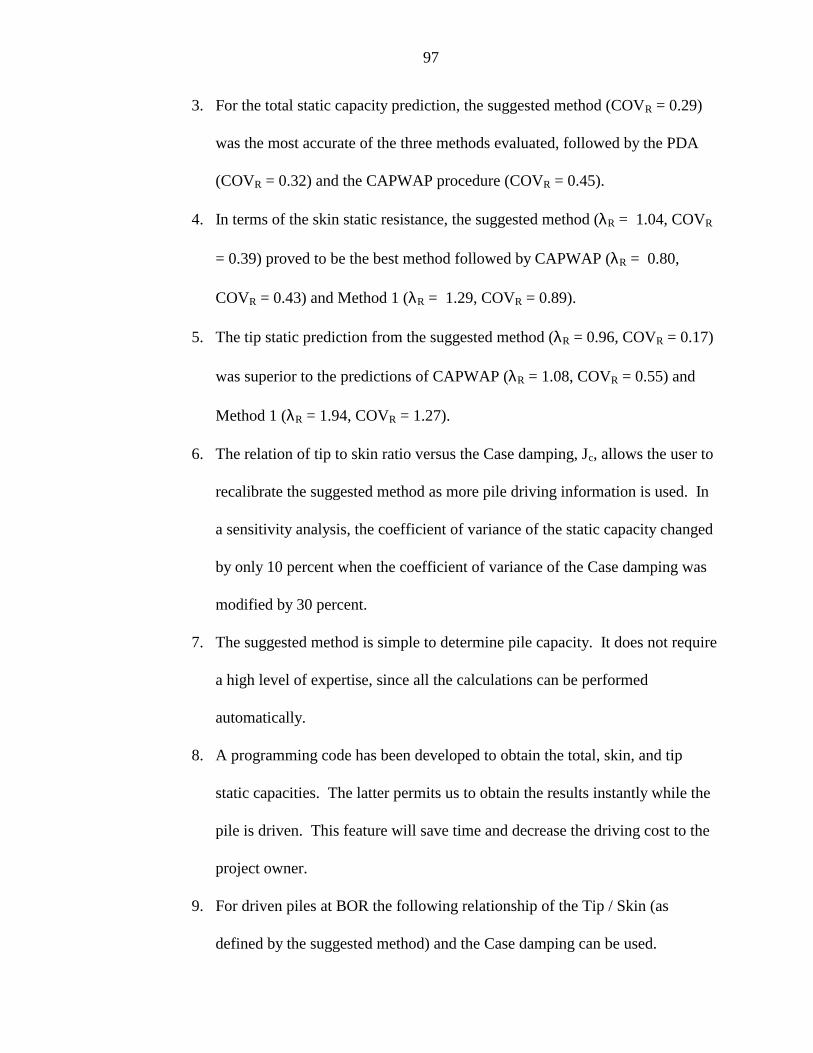
97
3. For the total static capacity prediction, the suggested method (COVR = 0.29)
was the most accurate of the three methods evaluated, followed by the PDA
(COVR = 0.32) and the CAPWAP procedure (COVR = 0.45).
4. In terms of the skin static resistance, the suggested method (λR = 1.04, COVR
= 0.39) proved to be the best method followed by CAPWAP (λR = 0.80,
COVR = 0.43) and Method 1 (λR = 1.29, COVR = 0.89).
5. The tip static prediction from the suggested method (λR = 0.96, COVR = 0.17)
was superior to the predictions of CAPWAP (λR = 1.08, COVR = 0.55) and
Method 1 (λR = 1.94, COVR = 1.27).
6. The relation of tip to skin ratio versus the Case damping, Jc, allows the user to
recalibrate the suggested method as more pile driving information is used. In
a sensitivity analysis, the coefficient of variance of the static capacity changed
by only 10 percent when the coefficient of variance of the Case damping was
modified by 30 percent.
7. The suggested method is simple to determine pile capacity. It does not require
a high level of expertise, since all the calculations can be performed
automatically.
8. A programming code has been developed to obtain the total, skin, and tip
static capacities. The latter permits us to obtain the results instantly while the
pile is driven. This feature will save time and decrease the driving cost to the
project owner.
9. For driven piles at BOR the following relationship of the Tip / Skin (as
defined by the suggested method) and the Case damping can be used.
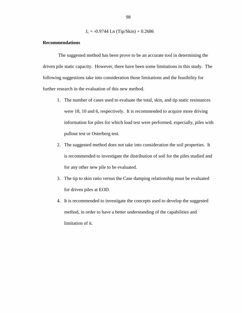
98
Jc = -0.9744 Ln (Tip/Skin) + 0.2686
Recommendations
The suggested method has been prove to be an accurate tool in determining the
driven pile static capacity. However, there have been some limitations in this study. The
following suggestions take into consideration those limitations and the feasibility for
further research in the evaluation of this new method.
1. The number of cases used to evaluate the total, skin, and tip static resistances
were 18, 10 and 6, respectively. It is recommended to acquire more driving
information for piles for which load test were performed, especially, piles with
pullout test or Osterberg test.
2. The suggested method does not take into consideration the soil properties. It
is recommended to investigate the distribution of soil for the piles studied and
for any other new pile to be evaluated.
3. The tip to skin ratio versus the Case damping relationship must be evaluated
for driven piles at EOD.
4. It is recommended to investigate the concepts used to develop the suggested
method, in order to have a better understanding of the capabilities and
limitation of it.

APPENDIX A
LRFD ANALYSIS RESULTS - CAPWAP PROCEDURE
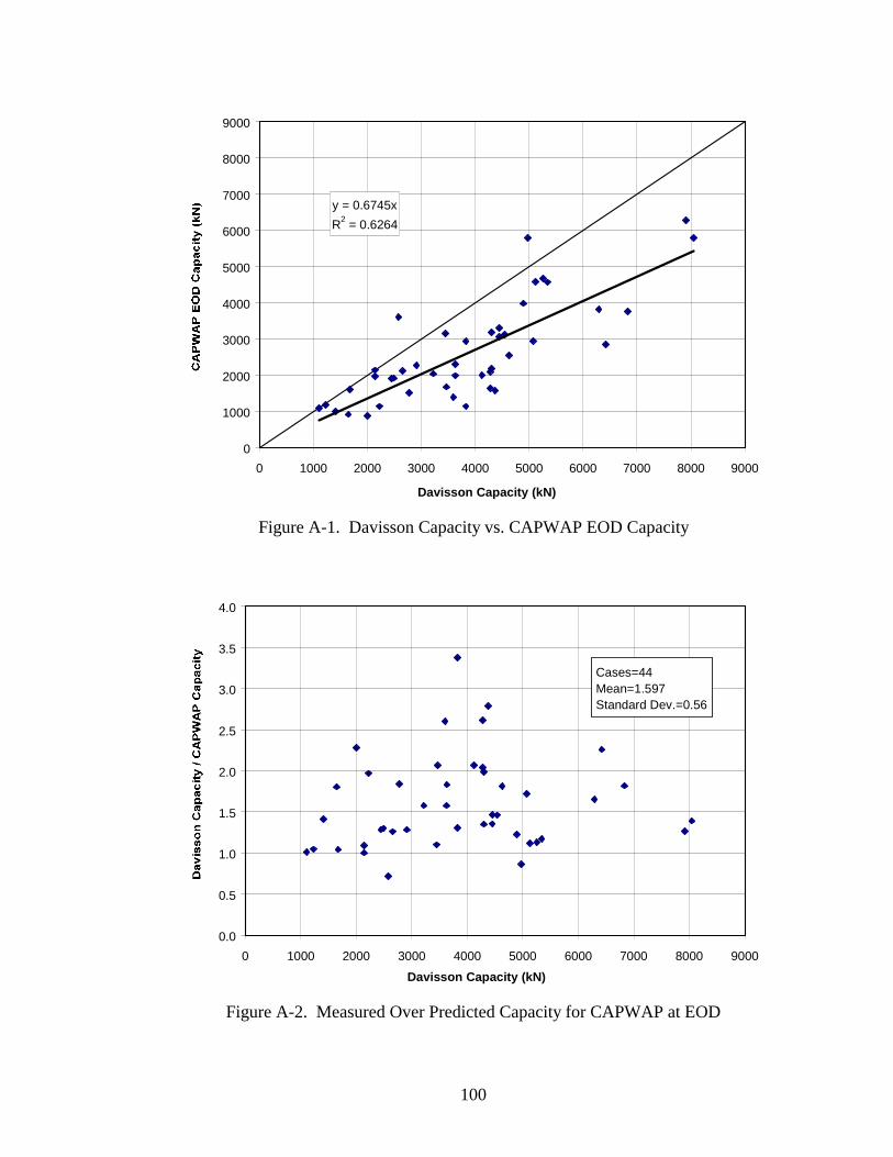
100
y = 0.6745x
R2 = 0.6264
0
1000
2000
3000
4000
5000
6000
7000
8000
9000
0 1000 2000 3000 4000 5000 6000 7000 8000 9000
Davisson Capacity (kN)
Figure A-1. Davisson Capacity vs. CAPWAP EOD Capacity
0.0
0.5
1.0
1.5
2.0
2.5
3.0
3.5
4.0
0 1000 2000 3000 4000 5000 6000 7000 8000 9000
Davisson Capacity (kN)
Cases=44Mean=1.597Standard Dev.=0.56
Figure A-2. Measured Over Predicted Capacity for CAPWAP at EOD

101
Table A-1. φ Values Evaluated for CAPWAP (EOD)
Span length Failure Probability pf / Reliability Index βΤ
(m) QD/QL 2.50E-02 6.22E-03 1.22E-03 1.79E-04
1.96 2.5 3.03 3.579 0.52 0.980 0.788 0.636 0.51115 1.00 0.940 0.756 0.610 0.49018 1.06 0.937 0.753 0.608 0.48927 1.58 0.912 0.733 0.591 0.47536 2.12 0.894 0.719 0.580 0.46645 2.64 0.882 0.709 0.572 0.46050 3.00 0.876 0.704 0.568 0.45760 3.53 0.868 0.698 0.563 0.453
Table A-2. ASD Design Safety Factor Values Evaluated for CAPWAP (EOD)
Span length Failure Probability pf / Reliability Index βΤ
(m) QD/QL 2.50E-02 6.22E-03 1.22E-03 1.79E-04
1.96 2.5 3.03 3.579 0.52 1.611 2.004 2.483 3.08915 1.00 1.595 1.984 2.459 3.05918 1.06 1.594 1.982 2.456 3.05627 1.58 1.584 1.970 2.441 3.03736 2.12 1.577 1.962 2.431 3.02445 2.64 1.572 1.956 2.424 3.01550 3.00 1.570 1.953 2.420 3.01160 3.53 1.567 1.949 2.415 3.005
Table A-3. φ Factors for Safety Factor = 2.50 – CAPWAP (EOD)
Span length(m) QD/QL φ βΤ pf
9 0.52 0.632 3.047 0.0011615 1.00 0.600 3.071 0.0010718 1.06 0.597 3.074 0.0010627 1.58 0.578 3.089 0.0010136 2.12 0.564 3.099 0.0009745 2.64 0.555 3.107 0.0009550 3.00 0.550 3.111 0.0009360 3.53 0.544 3.115 0.00092
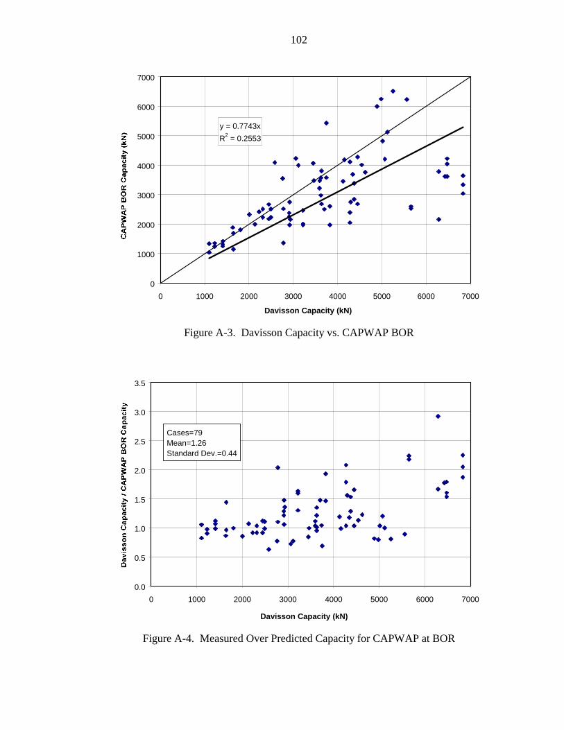
102
y = 0.7743x
R2 = 0.2553
0
1000
2000
3000
4000
5000
6000
7000
0 1000 2000 3000 4000 5000 6000 7000
Davisson Capacity (kN)
Figure A-3. Davisson Capacity vs. CAPWAP BOR
0.0
0.5
1.0
1.5
2.0
2.5
3.0
3.5
0 1000 2000 3000 4000 5000 6000 7000
Davisson Capacity (kN)
Cases=79Mean=1.26Standard Dev.=0.44
Figure A-4. Measured Over Predicted Capacity for CAPWAP at BOR
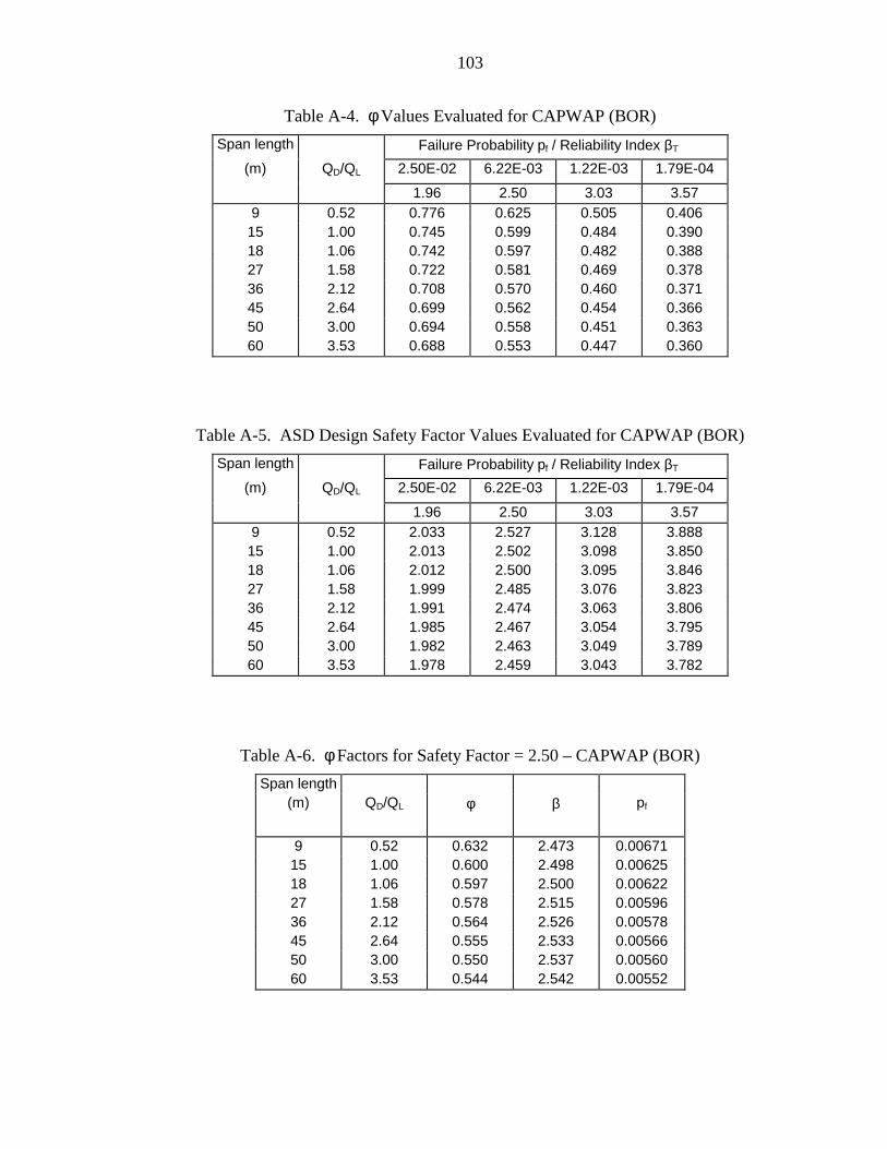
103
Table A-4. φ Values Evaluated for CAPWAP (BOR)
Span length Failure Probability pf / Reliability Index βΤ
(m) QD/QL 2.50E-02 6.22E-03 1.22E-03 1.79E-04
1.96 2.50 3.03 3.579 0.52 0.776 0.625 0.505 0.40615 1.00 0.745 0.599 0.484 0.39018 1.06 0.742 0.597 0.482 0.38827 1.58 0.722 0.581 0.469 0.37836 2.12 0.708 0.570 0.460 0.37145 2.64 0.699 0.562 0.454 0.36650 3.00 0.694 0.558 0.451 0.36360 3.53 0.688 0.553 0.447 0.360
Table A-5. ASD Design Safety Factor Values Evaluated for CAPWAP (BOR)
Span length Failure Probability pf / Reliability Index βΤ
(m) QD/QL 2.50E-02 6.22E-03 1.22E-03 1.79E-04
1.96 2.50 3.03 3.579 0.52 2.033 2.527 3.128 3.88815 1.00 2.013 2.502 3.098 3.85018 1.06 2.012 2.500 3.095 3.84627 1.58 1.999 2.485 3.076 3.82336 2.12 1.991 2.474 3.063 3.80645 2.64 1.985 2.467 3.054 3.79550 3.00 1.982 2.463 3.049 3.78960 3.53 1.978 2.459 3.043 3.782
Table A-6. φ Factors for Safety Factor = 2.50 – CAPWAP (BOR)
Span length(m) QD/QL φ β pf
9 0.52 0.632 2.473 0.0067115 1.00 0.600 2.498 0.0062518 1.06 0.597 2.500 0.0062227 1.58 0.578 2.515 0.0059636 2.12 0.564 2.526 0.0057845 2.64 0.555 2.533 0.0056650 3.00 0.550 2.537 0.0056060 3.53 0.544 2.542 0.00552

APPENDIX B
LRFD ANALYSIS RESULTS – PDA METHOD
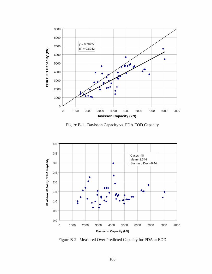
105
y = 0.7822x
R2 = 0.6042
0
1000
2000
3000
4000
5000
6000
7000
8000
9000
0 1000 2000 3000 4000 5000 6000 7000 8000 9000
Davisson Capacity (kN)
Figure B-1. Davisson Capacity vs. PDA EOD Capacity
0.0
0.5
1.0
1.5
2.0
2.5
3.0
3.5
4.0
0 1000 2000 3000 4000 5000 6000 7000 8000 9000
Davisson Capacity (kN)
Cases=48Mean=1.344Standard Dev.=0.44
Figure B-2. Measured Over Predicted Capacity for PDA at EOD
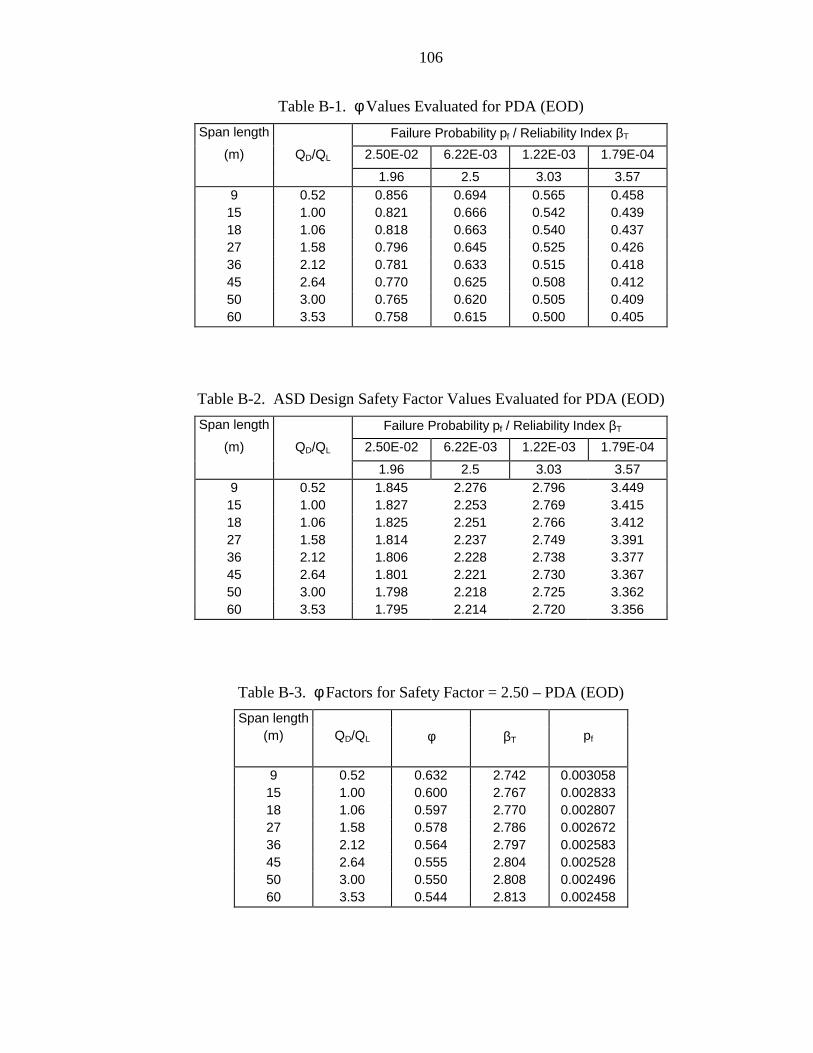
106
Table B-1. φ Values Evaluated for PDA (EOD)
Span length Failure Probability pf / Reliability Index βΤ
(m) QD/QL 2.50E-02 6.22E-03 1.22E-03 1.79E-04
1.96 2.5 3.03 3.579 0.52 0.856 0.694 0.565 0.45815 1.00 0.821 0.666 0.542 0.43918 1.06 0.818 0.663 0.540 0.43727 1.58 0.796 0.645 0.525 0.42636 2.12 0.781 0.633 0.515 0.41845 2.64 0.770 0.625 0.508 0.41250 3.00 0.765 0.620 0.505 0.40960 3.53 0.758 0.615 0.500 0.405
Table B-2. ASD Design Safety Factor Values Evaluated for PDA (EOD)
Span length Failure Probability pf / Reliability Index βΤ
(m) QD/QL 2.50E-02 6.22E-03 1.22E-03 1.79E-04
1.96 2.5 3.03 3.579 0.52 1.845 2.276 2.796 3.44915 1.00 1.827 2.253 2.769 3.41518 1.06 1.825 2.251 2.766 3.41227 1.58 1.814 2.237 2.749 3.39136 2.12 1.806 2.228 2.738 3.37745 2.64 1.801 2.221 2.730 3.36750 3.00 1.798 2.218 2.725 3.36260 3.53 1.795 2.214 2.720 3.356
Table B-3. φ Factors for Safety Factor = 2.50 – PDA (EOD)
Span length(m) QD/QL φ βΤ pf
9 0.52 0.632 2.742 0.00305815 1.00 0.600 2.767 0.00283318 1.06 0.597 2.770 0.00280727 1.58 0.578 2.786 0.00267236 2.12 0.564 2.797 0.00258345 2.64 0.555 2.804 0.00252850 3.00 0.550 2.808 0.00249660 3.53 0.544 2.813 0.002458
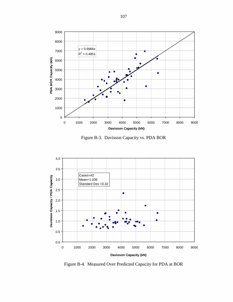
107
y = 0.9966x
R2 = 0.4851
0
1000
2000
3000
4000
5000
6000
7000
8000
9000
0 1000 2000 3000 4000 5000 6000 7000 8000 9000
Davisson Capacity (kN)
Figure B-3. Davisson Capacity vs. PDA BOR
0.0
0.5
1.0
1.5
2.0
2.5
3.0
3.5
4.0
0 1000 2000 3000 4000 5000 6000 7000 8000 9000
Davisson Capacity (kN)
Cases=42Mean=1.036Standard Dev.=0.32
Figure B-4. Measured Over Predicted Capacity for PDA at BOR
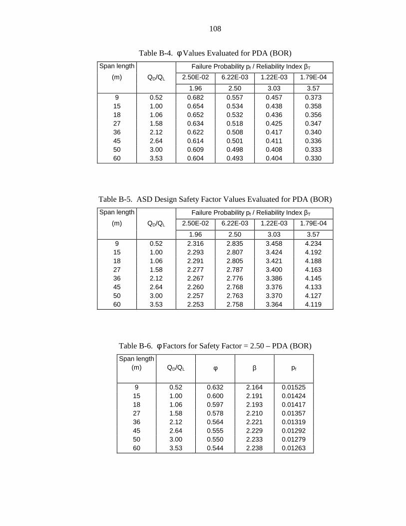
108
Table B-4. φ Values Evaluated for PDA (BOR)
Span length Failure Probability pf / Reliability Index βΤ
(m) QD/QL 2.50E-02 6.22E-03 1.22E-03 1.79E-04
1.96 2.50 3.03 3.579 0.52 0.682 0.557 0.457 0.37315 1.00 0.654 0.534 0.438 0.35818 1.06 0.652 0.532 0.436 0.35627 1.58 0.634 0.518 0.425 0.34736 2.12 0.622 0.508 0.417 0.34045 2.64 0.614 0.501 0.411 0.33650 3.00 0.609 0.498 0.408 0.33360 3.53 0.604 0.493 0.404 0.330
Table B-5. ASD Design Safety Factor Values Evaluated for PDA (BOR)
Span length Failure Probability pf / Reliability Index βΤ
(m) QD/QL 2.50E-02 6.22E-03 1.22E-03 1.79E-04
1.96 2.50 3.03 3.579 0.52 2.316 2.835 3.458 4.23415 1.00 2.293 2.807 3.424 4.19218 1.06 2.291 2.805 3.421 4.18827 1.58 2.277 2.787 3.400 4.16336 2.12 2.267 2.776 3.386 4.14545 2.64 2.260 2.768 3.376 4.13350 3.00 2.257 2.763 3.370 4.12760 3.53 2.253 2.758 3.364 4.119
Table B-6. φ Factors for Safety Factor = 2.50 – PDA (BOR)
Span length(m) QD/QL φ β pf
9 0.52 0.632 2.164 0.0152515 1.00 0.600 2.191 0.0142418 1.06 0.597 2.193 0.0141727 1.58 0.578 2.210 0.0135736 2.12 0.564 2.221 0.0131945 2.64 0.555 2.229 0.0129250 3.00 0.550 2.233 0.0127960 3.53 0.544 2.238 0.01263

APPENDIX C
LRFD ANALYSIS RESULTS – PAIKOWSKY’S ENERGY METHOD
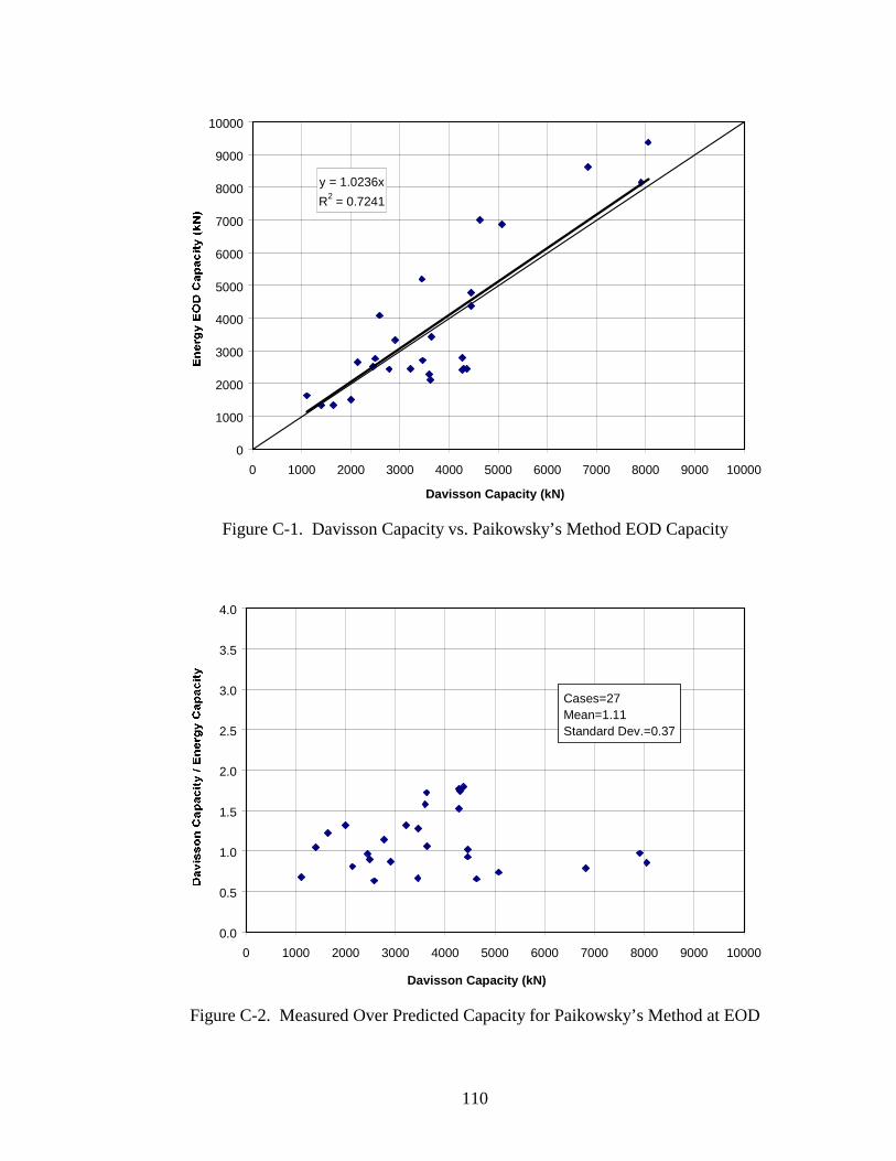
110
y = 1.0236x
R2 = 0.7241
0
1000
2000
3000
4000
5000
6000
7000
8000
9000
10000
0 1000 2000 3000 4000 5000 6000 7000 8000 9000 10000
Davisson Capacity (kN)
Figure C-1. Davisson Capacity vs. Paikowsky’s Method EOD Capacity
0.0
0.5
1.0
1.5
2.0
2.5
3.0
3.5
4.0
0 1000 2000 3000 4000 5000 6000 7000 8000 9000 10000
Davisson Capacity (kN)
Cases=27Mean=1.11Standard Dev.=0.37
Figure C-2. Measured Over Predicted Capacity for Paikowsky’s Method at EOD
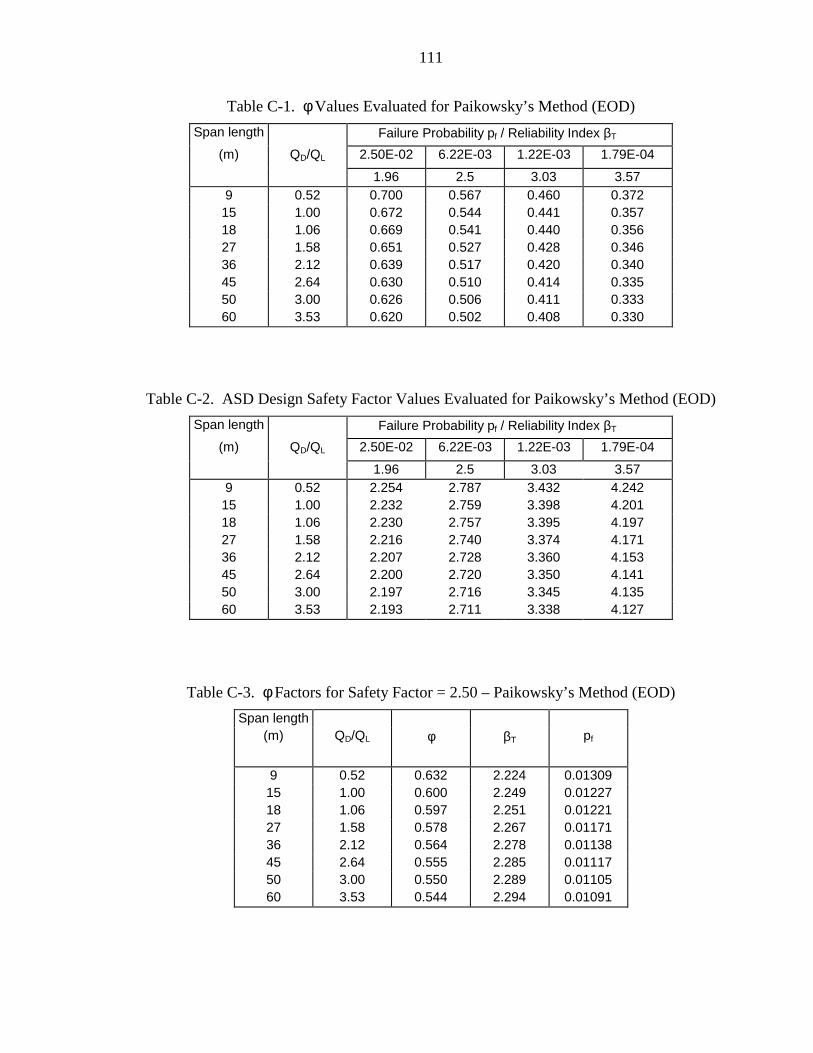
111
Table C-1. φ Values Evaluated for Paikowsky’s Method (EOD)
Span length Failure Probability pf / Reliability Index βΤ
(m) QD/QL 2.50E-02 6.22E-03 1.22E-03 1.79E-04
1.96 2.5 3.03 3.579 0.52 0.700 0.567 0.460 0.37215 1.00 0.672 0.544 0.441 0.35718 1.06 0.669 0.541 0.440 0.35627 1.58 0.651 0.527 0.428 0.34636 2.12 0.639 0.517 0.420 0.34045 2.64 0.630 0.510 0.414 0.33550 3.00 0.626 0.506 0.411 0.33360 3.53 0.620 0.502 0.408 0.330
Table C-2. ASD Design Safety Factor Values Evaluated for Paikowsky’s Method (EOD)
Span length Failure Probability pf / Reliability Index βΤ
(m) QD/QL 2.50E-02 6.22E-03 1.22E-03 1.79E-04
1.96 2.5 3.03 3.579 0.52 2.254 2.787 3.432 4.24215 1.00 2.232 2.759 3.398 4.20118 1.06 2.230 2.757 3.395 4.19727 1.58 2.216 2.740 3.374 4.17136 2.12 2.207 2.728 3.360 4.15345 2.64 2.200 2.720 3.350 4.14150 3.00 2.197 2.716 3.345 4.13560 3.53 2.193 2.711 3.338 4.127
Table C-3. φ Factors for Safety Factor = 2.50 – Paikowsky’s Method (EOD)
Span length(m) QD/QL φ βΤ pf
9 0.52 0.632 2.224 0.0130915 1.00 0.600 2.249 0.0122718 1.06 0.597 2.251 0.0122127 1.58 0.578 2.267 0.0117136 2.12 0.564 2.278 0.0113845 2.64 0.555 2.285 0.0111750 3.00 0.550 2.289 0.0110560 3.53 0.544 2.294 0.01091
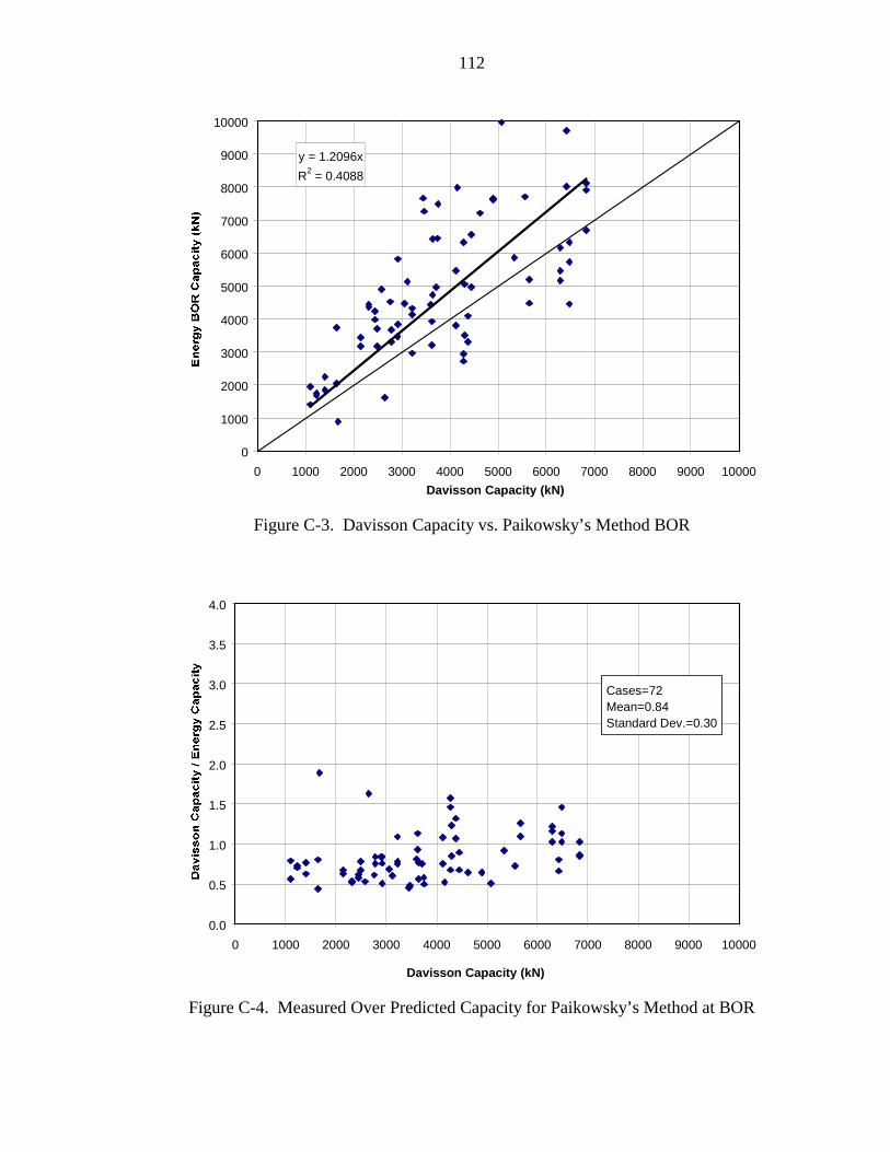
112
y = 1.2096x
R2 = 0.4088
0
1000
2000
3000
4000
5000
6000
7000
8000
9000
10000
0 1000 2000 3000 4000 5000 6000 7000 8000 9000 10000
Davisson Capacity (kN)
Figure C-3. Davisson Capacity vs. Paikowsky’s Method BOR
0.0
0.5
1.0
1.5
2.0
2.5
3.0
3.5
4.0
0 1000 2000 3000 4000 5000 6000 7000 8000 9000 10000
Davisson Capacity (kN)
Cases=72Mean=0.84Standard Dev.=0.30
Figure C-4. Measured Over Predicted Capacity for Paikowsky’s Method at BOR

113
Table C-4. φ Values Evaluated for Paikowsky’s Method (BOR)
Span length Failure Probability pf / Reliability Index βΤ
(m) QD/QL 2.50E-02 6.22E-03 1.22E-03 1.79E-04
1.96 2.50 3.03 3.579 0.52 0.503 0.403 0.323 0.25915 1.00 0.483 0.386 0.310 0.24818 1.06 0.481 0.385 0.309 0.24727 1.58 0.468 0.374 0.301 0.24136 2.12 0.459 0.367 0.295 0.23645 2.64 0.453 0.362 0.291 0.23350 3.00 0.449 0.360 0.289 0.23160 3.53 0.445 0.356 0.286 0.229
Table C-5. ASD Design Safety Factor Values Evaluated for Paikowsky’s Method (BOR)
Span length Failure Probability pf / Reliability Index βΤ
(m) QD/QL 2.50E-02 6.22E-03 1.22E-03 1.79E-04
1.96 2.50 3.03 3.579 0.52 3.139 3.923 4.881 6.10015 1.00 3.108 3.884 4.834 6.04018 1.06 3.105 3.881 4.829 6.03427 1.58 3.086 3.857 4.799 5.99736 2.12 3.073 3.840 4.779 5.97245 2.64 3.064 3.829 4.765 5.95550 3.00 3.059 3.823 4.758 5.94560 3.53 3.054 3.816 4.749 5.934
Table C-6. φ Factors for Safety Factor = 2.50 – Paikowsky’s Method (BOR)
Span length(m) QD/QL φ β pf
9 0.52 0.632 1.408 0.0796415 1.00 0.600 1.432 0.0761418 1.06 0.597 1.434 0.0758627 1.58 0.578 1.449 0.0737436 2.12 0.564 1.460 0.0722145 2.64 0.555 1.467 0.0712650 3.00 0.550 1.471 0.0707160 3.53 0.544 1.475 0.07017

APPENDIX D
LRFD ANALYSIS RESULTS – SAKAI ET AL (JAPANESE) METHOD
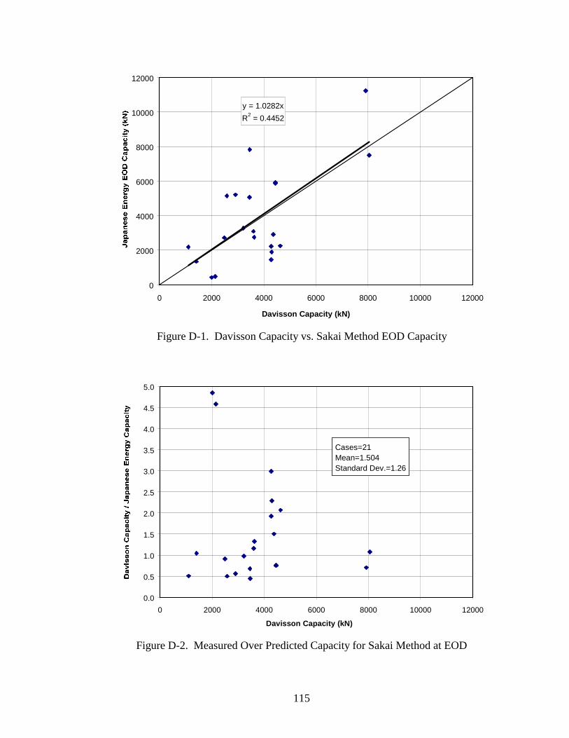
115
y = 1.0282x
R2 = 0.4452
0
2000
4000
6000
8000
10000
12000
0 2000 4000 6000 8000 10000 12000
Davisson Capacity (kN)
Figure D-1. Davisson Capacity vs. Sakai Method EOD Capacity
0.0
0.5
1.0
1.5
2.0
2.5
3.0
3.5
4.0
4.5
5.0
0 2000 4000 6000 8000 10000 12000
Davisson Capacity (kN)
Cases=21Mean=1.504Standard Dev.=1.26
Figure D-2. Measured Over Predicted Capacity for Sakai Method at EOD
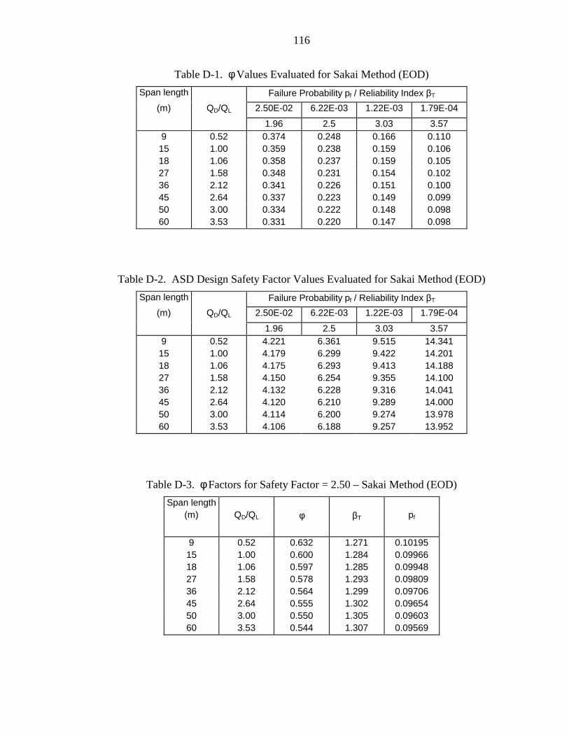
116
Table D-1. φ Values Evaluated for Sakai Method (EOD)
Span length Failure Probability pf / Reliability Index βΤ
(m) QD/QL 2.50E-02 6.22E-03 1.22E-03 1.79E-04
1.96 2.5 3.03 3.579 0.52 0.374 0.248 0.166 0.11015 1.00 0.359 0.238 0.159 0.10618 1.06 0.358 0.237 0.159 0.10527 1.58 0.348 0.231 0.154 0.10236 2.12 0.341 0.226 0.151 0.10045 2.64 0.337 0.223 0.149 0.09950 3.00 0.334 0.222 0.148 0.09860 3.53 0.331 0.220 0.147 0.098
Table D-2. ASD Design Safety Factor Values Evaluated for Sakai Method (EOD)
Span length Failure Probability pf / Reliability Index βΤ
(m) QD/QL 2.50E-02 6.22E-03 1.22E-03 1.79E-04
1.96 2.5 3.03 3.579 0.52 4.221 6.361 9.515 14.34115 1.00 4.179 6.299 9.422 14.20118 1.06 4.175 6.293 9.413 14.18827 1.58 4.150 6.254 9.355 14.10036 2.12 4.132 6.228 9.316 14.04145 2.64 4.120 6.210 9.289 14.00050 3.00 4.114 6.200 9.274 13.97860 3.53 4.106 6.188 9.257 13.952
Table D-3. φ Factors for Safety Factor = 2.50 – Sakai Method (EOD)
Span length(m) QD/QL φ βΤ pf
9 0.52 0.632 1.271 0.1019515 1.00 0.600 1.284 0.0996618 1.06 0.597 1.285 0.0994827 1.58 0.578 1.293 0.0980936 2.12 0.564 1.299 0.0970645 2.64 0.555 1.302 0.0965450 3.00 0.550 1.305 0.0960360 3.53 0.544 1.307 0.09569
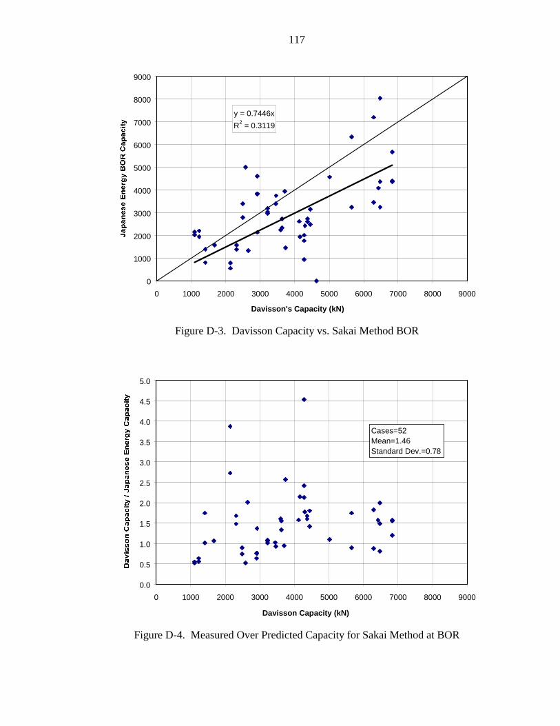
117
y = 0.7446x
R2 = 0.3119
0
1000
2000
3000
4000
5000
6000
7000
8000
9000
0 1000 2000 3000 4000 5000 6000 7000 8000 9000
Davisson's Capacity (kN)
Figure D-3. Davisson Capacity vs. Sakai Method BOR
0.0
0.5
1.0
1.5
2.0
2.5
3.0
3.5
4.0
4.5
5.0
0 1000 2000 3000 4000 5000 6000 7000 8000 9000
Davisson Capacity (kN)
Cases=52Mean=1.46Standard Dev.=0.78
Figure D-4. Measured Over Predicted Capacity for Sakai Method at BOR
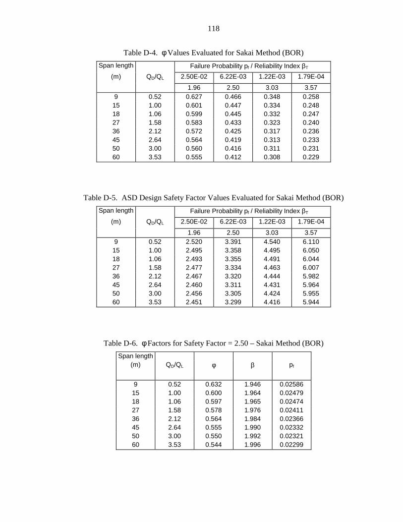
118
Table D-4. φ Values Evaluated for Sakai Method (BOR)
Span length Failure Probability pf / Reliability Index βΤ
(m) QD/QL 2.50E-02 6.22E-03 1.22E-03 1.79E-04
1.96 2.50 3.03 3.579 0.52 0.627 0.466 0.348 0.25815 1.00 0.601 0.447 0.334 0.24818 1.06 0.599 0.445 0.332 0.24727 1.58 0.583 0.433 0.323 0.24036 2.12 0.572 0.425 0.317 0.23645 2.64 0.564 0.419 0.313 0.23350 3.00 0.560 0.416 0.311 0.23160 3.53 0.555 0.412 0.308 0.229
Table D-5. ASD Design Safety Factor Values Evaluated for Sakai Method (BOR)
Span length Failure Probability pf / Reliability Index βΤ
(m) QD/QL 2.50E-02 6.22E-03 1.22E-03 1.79E-04
1.96 2.50 3.03 3.579 0.52 2.520 3.391 4.540 6.11015 1.00 2.495 3.358 4.495 6.05018 1.06 2.493 3.355 4.491 6.04427 1.58 2.477 3.334 4.463 6.00736 2.12 2.467 3.320 4.444 5.98245 2.64 2.460 3.311 4.431 5.96450 3.00 2.456 3.305 4.424 5.95560 3.53 2.451 3.299 4.416 5.944
Table D-6. φ Factors for Safety Factor = 2.50 – Sakai Method (BOR)
Span length(m) QD/QL φ β pf
9 0.52 0.632 1.946 0.0258615 1.00 0.600 1.964 0.0247918 1.06 0.597 1.965 0.0247427 1.58 0.578 1.976 0.0241136 2.12 0.564 1.984 0.0236645 2.64 0.555 1.990 0.0233250 3.00 0.550 1.992 0.0232160 3.53 0.544 1.996 0.02299

APPENDIX E
LRFD ANALYSIS RESULTS – FDOT METHOD
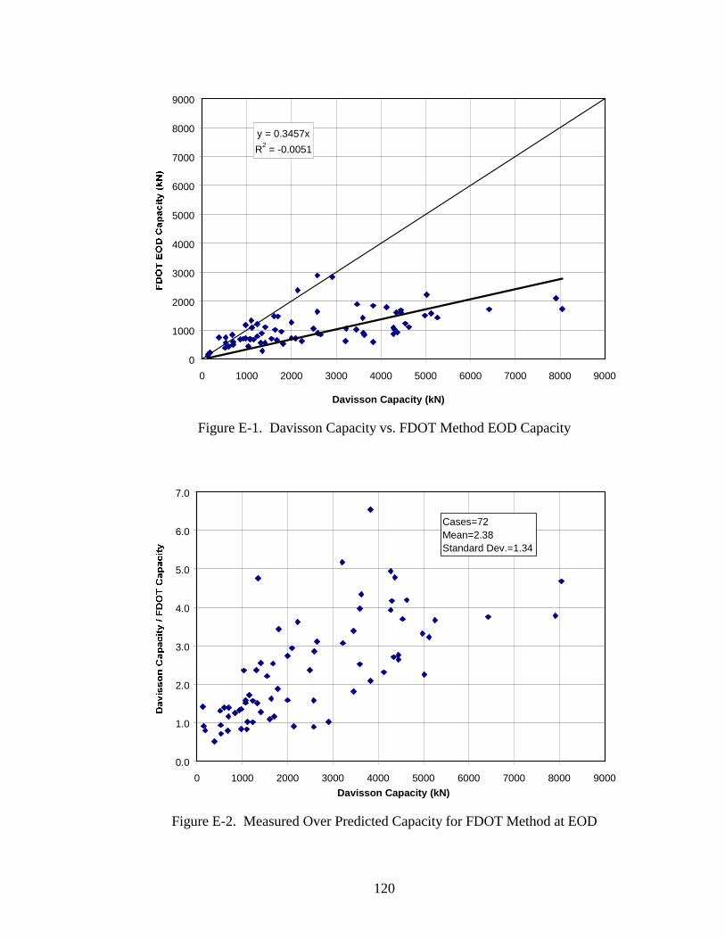
120
y = 0.3457x
R2 = -0.0051
0
1000
2000
3000
4000
5000
6000
7000
8000
9000
0 1000 2000 3000 4000 5000 6000 7000 8000 9000
Davisson Capacity (kN)
Figure E-1. Davisson Capacity vs. FDOT Method EOD Capacity
0.0
1.0
2.0
3.0
4.0
5.0
6.0
7.0
0 1000 2000 3000 4000 5000 6000 7000 8000 9000
Davisson Capacity (kN)
Cases=72Mean=2.38Standard Dev.=1.34
Figure E-2. Measured Over Predicted Capacity for FDOT Method at EOD
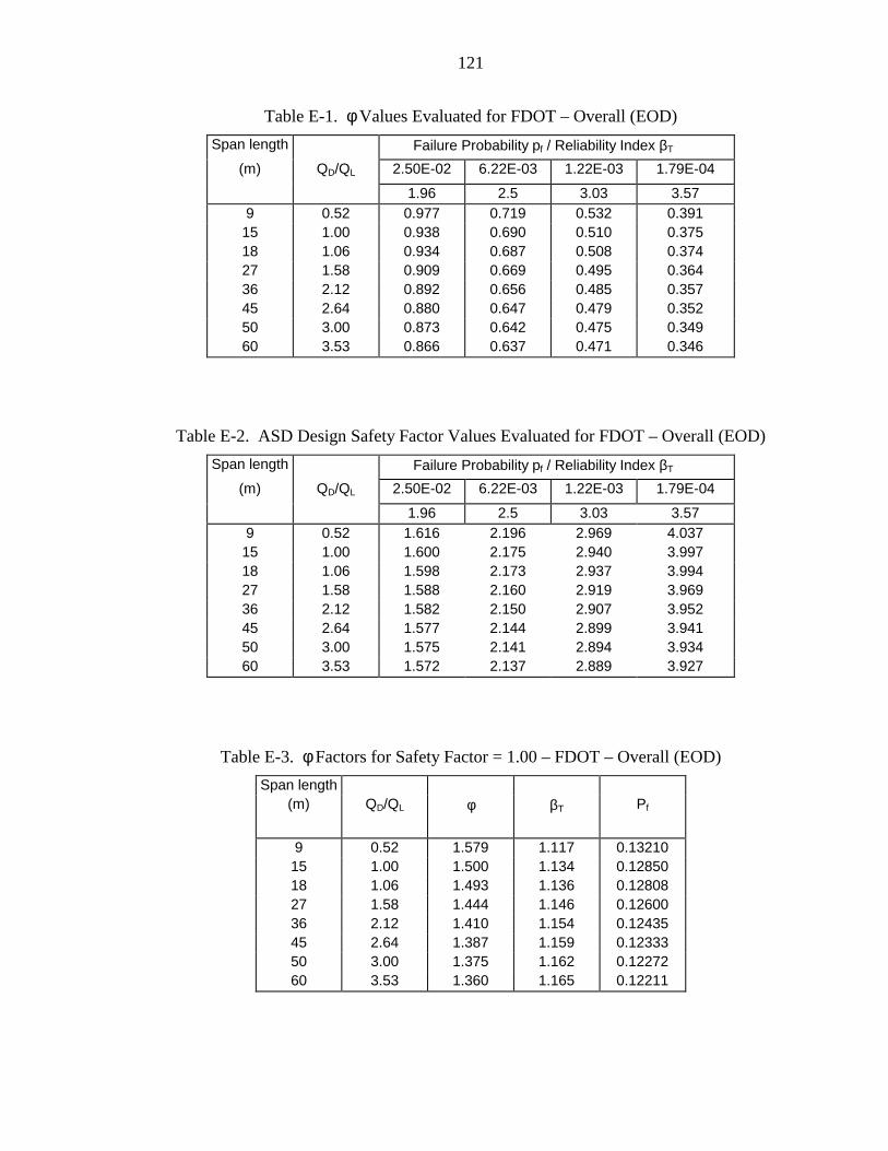
121
Table E-1. φ Values Evaluated for FDOT – Overall (EOD)
Span length Failure Probability pf / Reliability Index βΤ
(m) QD/QL 2.50E-02 6.22E-03 1.22E-03 1.79E-04
1.96 2.5 3.03 3.579 0.52 0.977 0.719 0.532 0.39115 1.00 0.938 0.690 0.510 0.37518 1.06 0.934 0.687 0.508 0.37427 1.58 0.909 0.669 0.495 0.36436 2.12 0.892 0.656 0.485 0.35745 2.64 0.880 0.647 0.479 0.35250 3.00 0.873 0.642 0.475 0.34960 3.53 0.866 0.637 0.471 0.346
Table E-2. ASD Design Safety Factor Values Evaluated for FDOT – Overall (EOD)
Span length Failure Probability pf / Reliability Index βΤ
(m) QD/QL 2.50E-02 6.22E-03 1.22E-03 1.79E-04
1.96 2.5 3.03 3.579 0.52 1.616 2.196 2.969 4.03715 1.00 1.600 2.175 2.940 3.99718 1.06 1.598 2.173 2.937 3.99427 1.58 1.588 2.160 2.919 3.96936 2.12 1.582 2.150 2.907 3.95245 2.64 1.577 2.144 2.899 3.94150 3.00 1.575 2.141 2.894 3.93460 3.53 1.572 2.137 2.889 3.927
Table E-3. φ Factors for Safety Factor = 1.00 – FDOT – Overall (EOD)
Span length(m) QD/QL φ βΤ Pf
9 0.52 1.579 1.117 0.1321015 1.00 1.500 1.134 0.1285018 1.06 1.493 1.136 0.1280827 1.58 1.444 1.146 0.1260036 2.12 1.410 1.154 0.1243545 2.64 1.387 1.159 0.1233350 3.00 1.375 1.162 0.1227260 3.53 1.360 1.165 0.12211

122
Table E-4. φ Values Evaluated for FDOT < 1779 kN (EOD)
Span length Failure Probability pf / Reliability Index βΤ
(m) QD/QL 2.50E-02 6.22E-03 1.22E-03 1.79E-04
1.96 2.5 3.03 3.579 0.52 0.657 0.491 0.369 0.27615 1.00 0.631 0.471 0.354 0.26418 1.06 0.628 0.469 0.352 0.26327 1.58 0.611 0.457 0.343 0.25636 2.12 0.600 0.448 0.336 0.25145 2.64 0.592 0.442 0.332 0.24850 3.00 0.587 0.439 0.330 0.24660 3.53 0.582 0.435 0.327 0.244
Table E-5. ASD Design Safety Factor Values Evaluated for FDOT < 1779 kN (EOD)
Span length Failure Probability pf / Reliability Index βΤ
(m) QD/QL 2.50E-02 6.22E-03 1.22E-03 1.79E-04
1.96 2.5 3.03 3.579 0.52 2.402 3.215 4.281 5.73015 1.00 2.378 3.184 4.239 5.67418 1.06 2.376 3.181 4.235 5.66927 1.58 2.362 3.161 4.209 5.63436 2.12 2.352 3.148 4.191 5.61045 2.64 2.345 3.139 4.179 5.59450 3.00 2.341 3.134 4.172 5.58560 3.53 2.337 3.128 4.164 5.575
Table E-6. φ Factors for Safety Factor = 1.00 – FDOT <1779 kN (EOD)
Span length(m) QD/QL φ βΤ pf
9 0.52 1.579 0.338 0.3678715 1.00 1.500 0.356 0.3611118 1.06 1.493 0.358 0.3603627 1.58 1.444 0.369 0.3562536 2.12 1.410 0.377 0.3532745 2.64 1.387 0.382 0.3514250 3.00 1.375 0.385 0.3503060 3.53 1.360 0.389 0.34882

123
Table E-7. φ Values Evaluated for FDOT > 1779 kN (EOD)
Span length Failure Probability pf / Reliability Index βΤ
(m) QD/QL 2.50E-02 6.22E-03 1.22E-03 1.79E-04
1.96 2.5 3.03 3.579 0.52 1.783 1.406 1.114 0.87815 1.00 1.710 1.349 1.068 0.84318 1.06 1.703 1.343 1.064 0.83927 1.58 1.658 1.307 1.036 0.81736 2.12 1.626 1.283 1.016 0.80145 2.64 1.604 1.265 1.002 0.79150 3.00 1.593 1.256 0.995 0.78560 3.53 1.579 1.245 0.986 0.778
Table E-8. ASD Design Safety Factor Values Evaluated for FDOT > 1779 kN (EOD)
Span length Failure Probability pf / Reliability Index βΤ
(m) QD/QL 2.50E-02 6.22E-03 1.22E-03 1.79E-04
1.96 2.5 3.03 3.579 0.52 0.886 1.123 1.418 1.79815 1.00 0.877 1.112 1.404 1.78018 1.06 0.876 1.111 1.403 1.77827 1.58 0.871 1.104 1.394 1.76736 2.12 0.867 1.100 1.388 1.76045 2.64 0.865 1.096 1.384 1.75550 3.00 0.863 1.095 1.382 1.75260 3.53 0.862 1.093 1.379 1.749
Table E-9. φ Factors for Safety Factor = 1.00 – FDOT >1779 kN (EOD)
Span length(m) QD/QL φ βΤ pf
9 0.52 1.579 2.236 0.0126915 1.00 1.500 2.258 0.0119918 1.06 1.493 2.260 0.0119327 1.58 1.444 2.274 0.0115036 2.12 1.410 2.284 0.0112045 2.64 1.387 2.291 0.0110050 3.00 1.375 2.294 0.0109160 3.53 1.360 2.299 0.01077
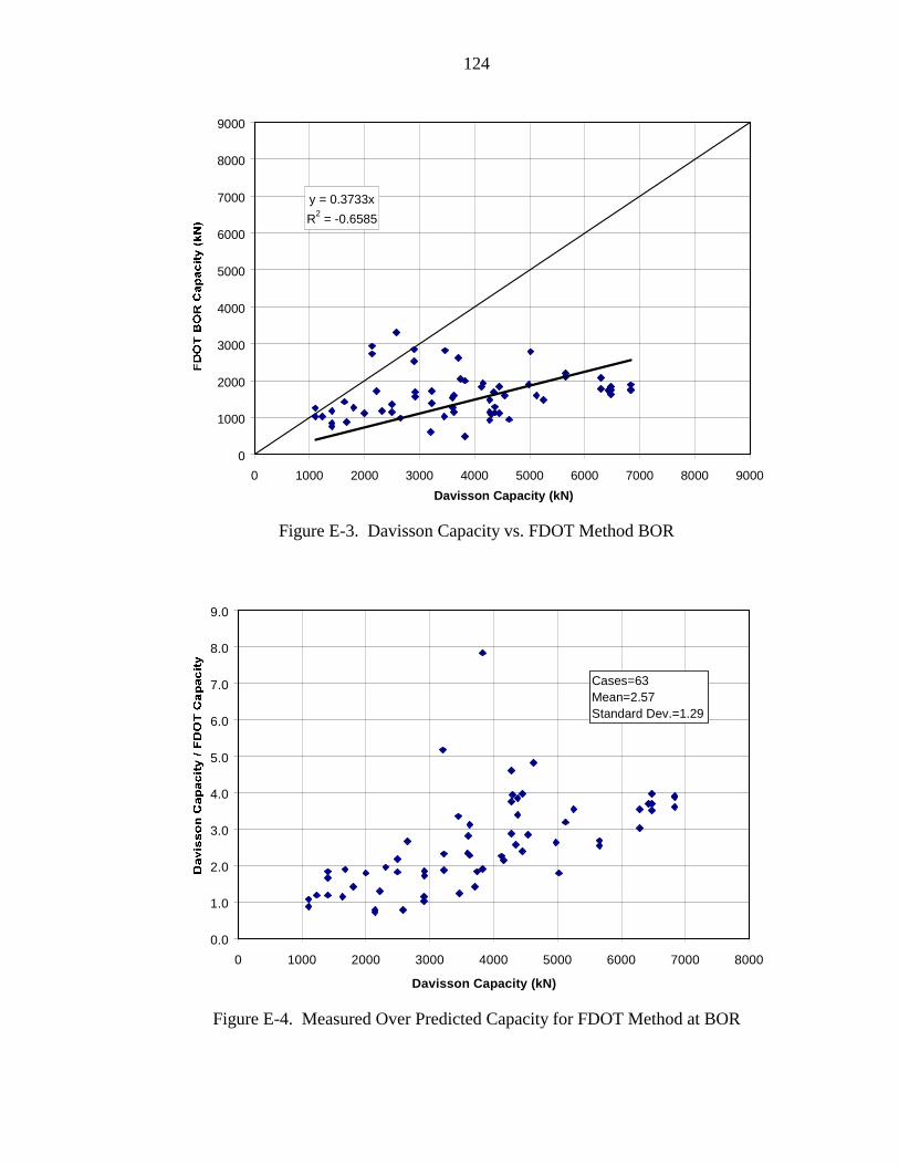
124
y = 0.3733x
R2 = -0.6585
0
1000
2000
3000
4000
5000
6000
7000
8000
9000
0 1000 2000 3000 4000 5000 6000 7000 8000 9000
Davisson Capacity (kN)
Figure E-3. Davisson Capacity vs. FDOT Method BOR
0.0
1.0
2.0
3.0
4.0
5.0
6.0
7.0
8.0
9.0
0 1000 2000 3000 4000 5000 6000 7000 8000
Davisson Capacity (kN)
Cases=63Mean=2.57Standard Dev.=1.29
Figure E-4. Measured Over Predicted Capacity for FDOT Method at BOR
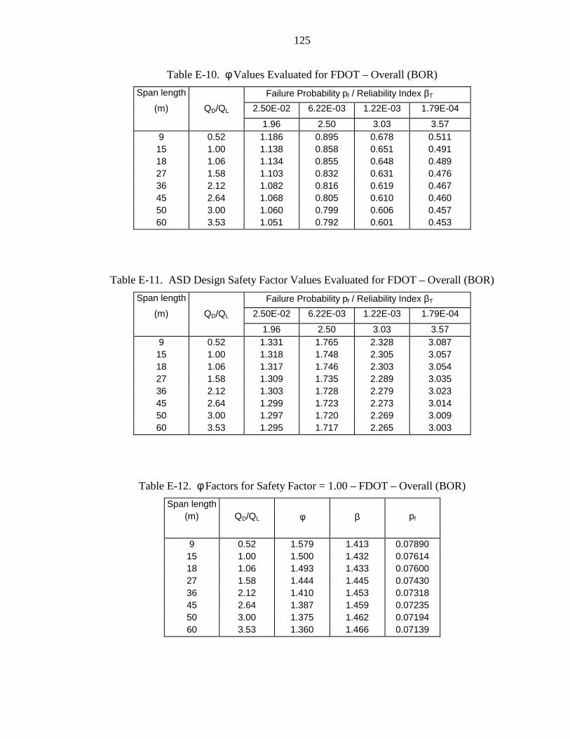
125
Table E-10. φ Values Evaluated for FDOT – Overall (BOR)
Span length Failure Probability pf / Reliability Index βΤ
(m) QD/QL 2.50E-02 6.22E-03 1.22E-03 1.79E-04
1.96 2.50 3.03 3.579 0.52 1.186 0.895 0.678 0.51115 1.00 1.138 0.858 0.651 0.49118 1.06 1.134 0.855 0.648 0.48927 1.58 1.103 0.832 0.631 0.47636 2.12 1.082 0.816 0.619 0.46745 2.64 1.068 0.805 0.610 0.46050 3.00 1.060 0.799 0.606 0.45760 3.53 1.051 0.792 0.601 0.453
Table E-11. ASD Design Safety Factor Values Evaluated for FDOT – Overall (BOR)
Span length Failure Probability pf / Reliability Index βΤ
(m) QD/QL 2.50E-02 6.22E-03 1.22E-03 1.79E-04
1.96 2.50 3.03 3.579 0.52 1.331 1.765 2.328 3.08715 1.00 1.318 1.748 2.305 3.05718 1.06 1.317 1.746 2.303 3.05427 1.58 1.309 1.735 2.289 3.03536 2.12 1.303 1.728 2.279 3.02345 2.64 1.299 1.723 2.273 3.01450 3.00 1.297 1.720 2.269 3.00960 3.53 1.295 1.717 2.265 3.003
Table E-12. φ Factors for Safety Factor = 1.00 – FDOT – Overall (BOR)
Span length(m) QD/QL φ β pf
9 0.52 1.579 1.413 0.0789015 1.00 1.500 1.432 0.0761418 1.06 1.493 1.433 0.0760027 1.58 1.444 1.445 0.0743036 2.12 1.410 1.453 0.0731845 2.64 1.387 1.459 0.0723550 3.00 1.375 1.462 0.0719460 3.53 1.360 1.466 0.07139

126
Table E-13. φ Values Evaluated for FDOT < 1779 kN (BOR)
Span length Failure Probability pf / Reliability Index βΤ
(m) QD/QL 2.50E-02 6.22E-03 1.22E-03 1.79E-04
1.96 2.50 3.03 3.579 0.52 0.941 0.778 0.646 0.53415 1.00 0.903 0.747 0.620 0.51218 1.06 0.899 0.744 0.617 0.51027 1.58 0.875 0.724 0.601 0.49736 2.12 0.858 0.710 0.589 0.48745 2.64 0.847 0.700 0.581 0.48150 3.00 0.841 0.695 0.577 0.47760 3.53 0.833 0.689 0.572 0.473
Table E-14. ASD Design Safety Factor Values Evaluated for FDOT < 1779 kN (BOR)
Span length Failure Probability pf / Reliability Index βΤ
(m) QD/QL 2.50E-02 6.22E-03 1.22E-03 1.79E-04
1.96 2.50 3.03 3.579 0.52 1.678 2.029 2.445 2.95615 1.00 1.662 2.009 2.421 2.92718 1.06 1.660 2.007 2.419 2.92527 1.58 1.650 1.995 2.404 2.90736 2.12 1.643 1.987 2.394 2.89445 2.64 1.638 1.981 2.387 2.88650 3.00 1.636 1.978 2.383 2.88160 3.53 1.633 1.974 2.378 2.876
Table E-15. φ Factors for Safety Factor = 1.00 – FDOT <1779 kN (BOR)
Span length(m) QD/QL φ β pf
9 0.52 1.579 0.488 0.313015 1.00 1.500 0.516 0.303118 1.06 1.493 0.519 0.302127 1.58 1.444 0.536 0.296236 2.12 1.410 0.548 0.292045 2.64 1.387 0.557 0.288950 3.00 1.375 0.561 0.287660 3.53 1.360 0.566 0.2859

127
Table E-16. φ Values Evaluated for FDOT > 1779 kN (BOR)
Span length Failure Probability pf / Reliability Index βΤ
(m) QD/QL 2.50E-02 6.22E-03 1.22E-03 1.79E-04
1.96 2.50 3.03 3.579 0.52 1.357 1.039 0.799 0.61115 1.00 1.302 0.996 0.766 0.58718 1.06 1.297 0.992 0.763 0.58427 1.58 1.262 0.966 0.743 0.56936 2.12 1.238 0.947 0.729 0.55845 2.64 1.221 0.935 0.719 0.55050 3.00 1.212 0.928 0.714 0.54660 3.53 1.202 0.920 0.708 0.542
Table E-17. ASD Design Safety Factor Values Evaluated for FDOT > 1779 kN (BOR)
Span length Failure Probability pf / Reliability Index βΤ
(m) QD/QL 2.50E-02 6.22E-03 1.22E-03 1.79E-04
1.96 2.50 3.03 3.579 0.52 1.164 1.520 1.976 2.58215 1.00 1.152 1.505 1.957 2.55718 1.06 1.151 1.504 1.955 2.55527 1.58 1.144 1.495 1.943 2.53936 2.12 1.139 1.488 1.935 2.52845 2.64 1.136 1.484 1.929 2.52150 3.00 1.134 1.482 1.926 2.51760 3.53 1.132 1.479 1.923 2.512
Table E-18. φ Factors for Safety Factor = 1.00 – FDOT >1779 kN (BOR)
Span length(m) QD/QL φ β pf
9 0.52 1.579 1.654 0.049115 1.00 1.500 1.674 0.047118 1.06 1.493 1.676 0.046927 1.58 1.444 1.688 0.045836 2.12 1.410 1.697 0.044945 2.64 1.387 1.703 0.044350 3.00 1.375 1.706 0.044160 3.53 1.360 1.710 0.0437

APPENDIX F
LRFD ANALYSIS RESULTS – ENGINEERING NEWS RECORD (ENR)
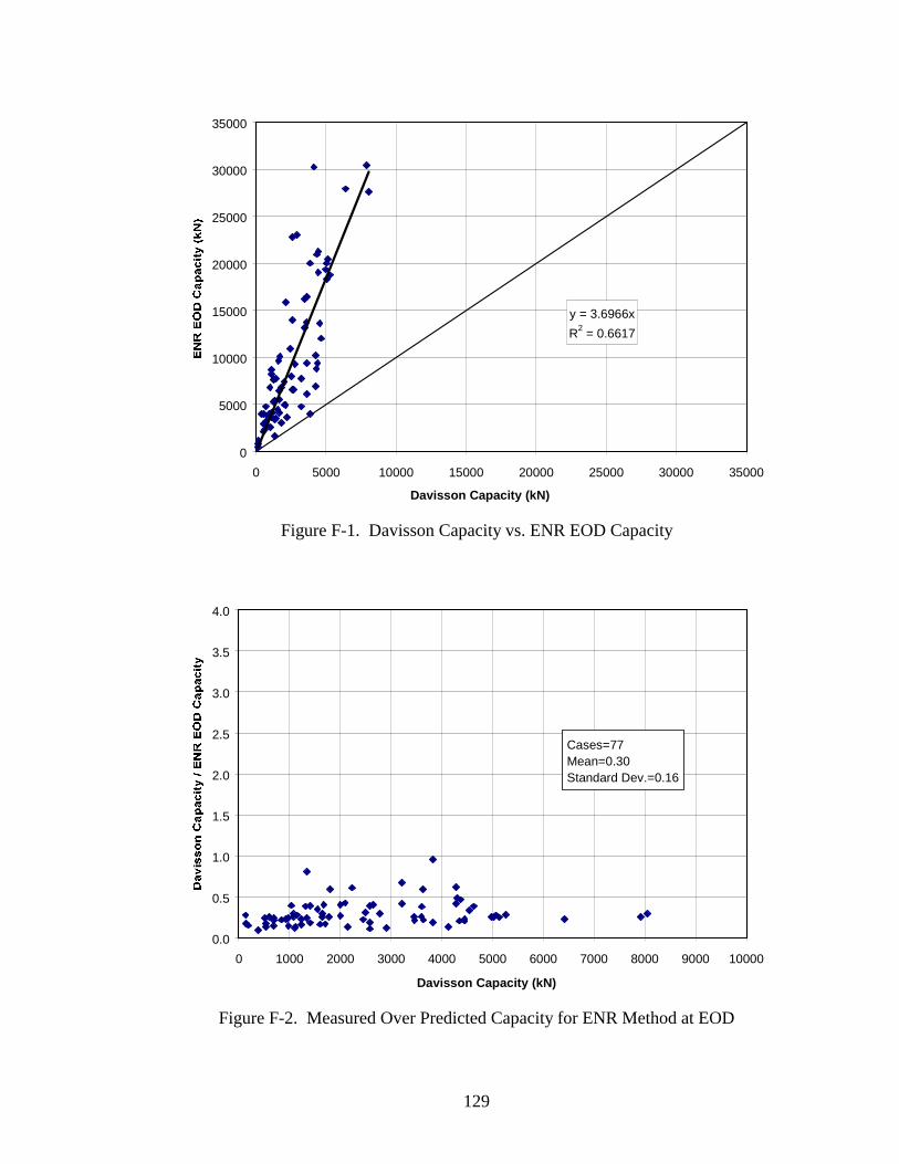
129
y = 3.6966x
R2 = 0.6617
0
5000
10000
15000
20000
25000
30000
35000
0 5000 10000 15000 20000 25000 30000 35000
Davisson Capacity (kN)
Figure F-1. Davisson Capacity vs. ENR EOD Capacity
0.0
0.5
1.0
1.5
2.0
2.5
3.0
3.5
4.0
0 1000 2000 3000 4000 5000 6000 7000 8000 9000 10000
Davisson Capacity (kN)
Cases=77Mean=0.30Standard Dev.=0.16
Figure F-2. Measured Over Predicted Capacity for ENR Method at EOD
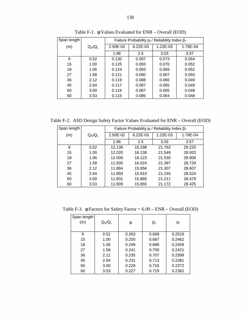
130
Table F-1. φ Values Evaluated for ENR – Overall (EOD)
Span length Failure Probability pf / Reliability Index βΤ
(m) QD/QL 2.50E-02 6.22E-03 1.22E-03 1.79E-04
1.96 2.5 3.03 3.579 0.52 0.130 0.097 0.073 0.05415 1.00 0.125 0.093 0.070 0.05218 1.06 0.124 0.093 0.069 0.05227 1.58 0.121 0.090 0.067 0.05036 2.12 0.119 0.088 0.066 0.04945 2.64 0.117 0.087 0.065 0.04950 3.00 0.116 0.087 0.065 0.04860 3.53 0.115 0.086 0.064 0.048
Table F-2. ASD Design Safety Factor Values Evaluated for ENR – Overall (EOD)
Span length Failure Probability pf / Reliability Index βΤ
(m) QD/QL 2.50E-02 6.22E-03 1.22E-03 1.79E-04
1.96 2.5 3.03 3.579 0.52 12.139 16.298 21.763 29.22015 1.00 12.020 16.138 21.549 28.93318 1.06 12.009 16.123 21.530 28.90627 1.58 11.935 16.024 21.397 28.72936 2.12 11.884 15.956 21.307 28.60745 2.64 11.850 15.910 21.245 28.52450 3.00 11.831 15.885 21.211 28.47960 3.53 11.809 15.855 21.172 28.425
Table F-3. φ Factors for Safety Factor = 6.00 – ENR – Overall (EOD)
Span length(m) QD/QL φ βΤ pf
9 0.52 0.263 0.669 0.251915 1.00 0.250 0.687 0.246218 1.06 0.249 0.688 0.245927 1.58 0.241 0.700 0.242136 2.12 0.235 0.707 0.239945 2.64 0.231 0.713 0.238150 3.00 0.229 0.716 0.237260 3.53 0.227 0.719 0.2362

131
Table F-4. φ Values Evaluated for ENR < 1779 kN (EOD)
Span length Failure Probability pf / Reliability Index βΤ
(m) QD/QL 2.50E-02 6.22E-03 1.22E-03 1.79E-04
1.96 2.5 3.03 3.579 0.52 0.112 0.084 0.064 0.04815 1.00 0.108 0.081 0.061 0.04618 1.06 0.107 0.081 0.061 0.04627 1.58 0.105 0.078 0.059 0.04436 2.12 0.103 0.077 0.058 0.04445 2.64 0.101 0.076 0.057 0.04350 3.00 0.101 0.075 0.057 0.04360 3.53 0.100 0.075 0.056 0.042
Table F-5. ASD Design Safety Factor Values Evaluated for ENR < 1779 kN (EOD)
Span length Failure Probability pf / Reliability Index βΤ
(m) QD/QL 2.50E-02 6.22E-03 1.22E-03 1.79E-04
1.96 2.5 3.03 3.579 0.52 14.037 18.709 24.806 33.06315 1.00 13.899 18.526 24.562 32.73918 1.06 13.886 18.509 24.540 32.70927 1.58 13.801 18.395 24.389 32.50836 2.12 13.742 18.317 24.285 32.37045 2.64 13.702 18.264 24.215 32.27650 3.00 13.681 18.235 24.177 32.22560 3.53 13.655 18.201 24.131 32.165
Table F-6. φ Factors for Safety Factor = 6.00 – ENR <1779 kN (EOD)
Span length(m) QD/QL φ βΤ pf
9 0.52 0.263 0.363 0.358515 1.00 0.250 0.381 0.351818 1.06 0.249 0.383 0.351027 1.58 0.241 0.395 0.346636 2.12 0.235 0.403 0.343745 2.64 0.231 0.408 0.341850 3.00 0.229 0.411 0.340760 3.53 0.227 0.415 0.3393
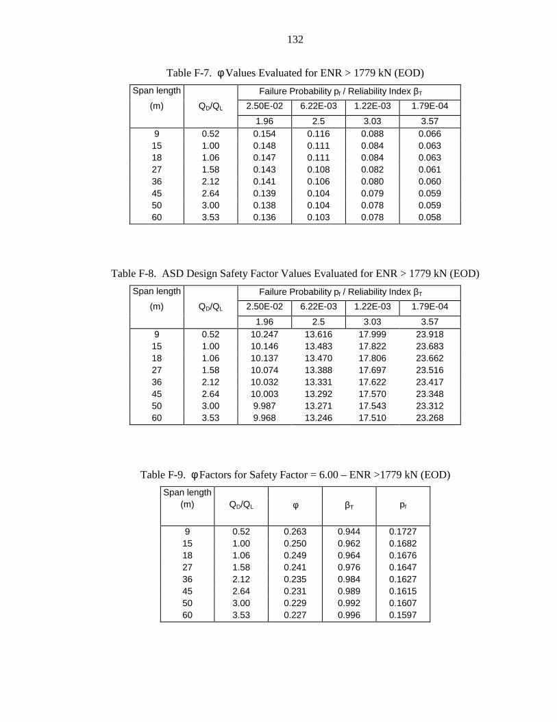
132
Table F-7. φ Values Evaluated for ENR > 1779 kN (EOD)
Span length Failure Probability pf / Reliability Index βΤ
(m) QD/QL 2.50E-02 6.22E-03 1.22E-03 1.79E-04
1.96 2.5 3.03 3.579 0.52 0.154 0.116 0.088 0.06615 1.00 0.148 0.111 0.084 0.06318 1.06 0.147 0.111 0.084 0.06327 1.58 0.143 0.108 0.082 0.06136 2.12 0.141 0.106 0.080 0.06045 2.64 0.139 0.104 0.079 0.05950 3.00 0.138 0.104 0.078 0.05960 3.53 0.136 0.103 0.078 0.058
Table F-8. ASD Design Safety Factor Values Evaluated for ENR > 1779 kN (EOD)
Span length Failure Probability pf / Reliability Index βΤ
(m) QD/QL 2.50E-02 6.22E-03 1.22E-03 1.79E-04
1.96 2.5 3.03 3.579 0.52 10.247 13.616 17.999 23.91815 1.00 10.146 13.483 17.822 23.68318 1.06 10.137 13.470 17.806 23.66227 1.58 10.074 13.388 17.697 23.51636 2.12 10.032 13.331 17.622 23.41745 2.64 10.003 13.292 17.570 23.34850 3.00 9.987 13.271 17.543 23.31260 3.53 9.968 13.246 17.510 23.268
Table F-9. φ Factors for Safety Factor = 6.00 – ENR >1779 kN (EOD)
Span length(m) QD/QL φ βΤ pf
9 0.52 0.263 0.944 0.172715 1.00 0.250 0.962 0.168218 1.06 0.249 0.964 0.167627 1.58 0.241 0.976 0.164736 2.12 0.235 0.984 0.162745 2.64 0.231 0.989 0.161550 3.00 0.229 0.992 0.160760 3.53 0.227 0.996 0.1597
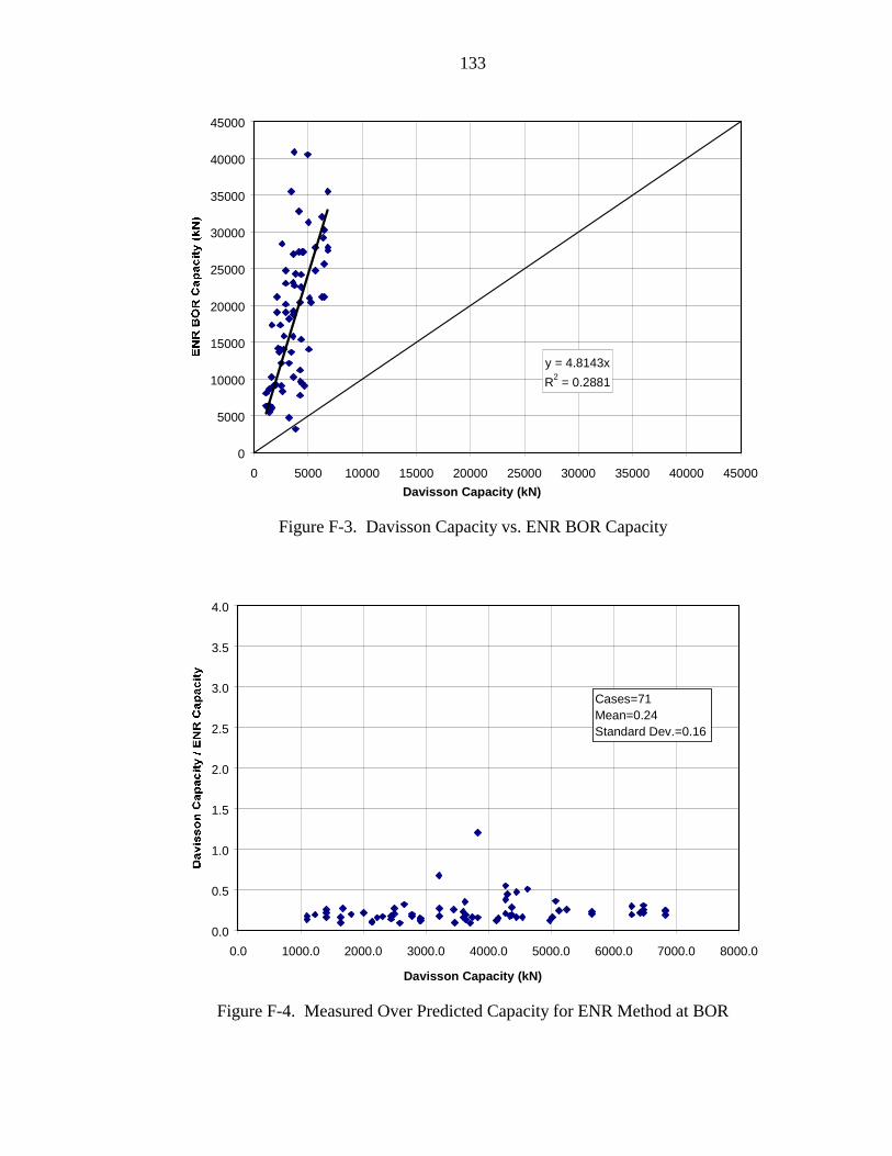
133
y = 4.8143x
R2 = 0.2881
0
5000
10000
15000
20000
25000
30000
35000
40000
45000
0 5000 10000 15000 20000 25000 30000 35000 40000 45000
Davisson Capacity (kN)
Figure F-3. Davisson Capacity vs. ENR BOR Capacity
0.0
0.5
1.0
1.5
2.0
2.5
3.0
3.5
4.0
0.0 1000.0 2000.0 3000.0 4000.0 5000.0 6000.0 7000.0 8000.0
Davisson Capacity (kN)
Cases=71Mean=0.24Standard Dev.=0.16
Figure F-4. Measured Over Predicted Capacity for ENR Method at BOR

134
Table F-10. φ Values Evaluated for ENR – Overall (BOR)
Span length Failure Probability pf / Reliability Index βΤ
(m) QD/QL 2.50E-02 6.22E-03 1.22E-03 1.79E-04
1.96 2.50 3.03 3.579 0.52 0.077 0.054 0.038 0.02715 1.00 0.074 0.052 0.037 0.02618 1.06 0.074 0.052 0.037 0.02627 1.58 0.072 0.050 0.036 0.02536 2.12 0.071 0.050 0.035 0.02545 2.64 0.070 0.049 0.035 0.02450 3.00 0.069 0.049 0.034 0.02460 3.53 0.068 0.048 0.034 0.024
Table F-11. ASD Design Safety Factor Values Evaluated for ENR – Overall (BOR)
Span length Failure Probability pf / Reliability Index βΤ
(m) QD/QL 2.50E-02 6.22E-03 1.22E-03 1.79E-04
1.96 2.50 3.03 3.579 0.52 20.423 29.086 41.153 58.60815 1.00 20.223 28.800 40.749 58.03318 1.06 20.204 28.774 40.712 57.98027 1.58 20.080 28.597 40.461 57.62336 2.12 19.995 28.476 40.290 57.37945 2.64 19.937 28.393 40.172 57.21250 3.00 19.905 28.348 40.109 57.12260 3.53 19.868 28.296 40.034 57.015
Table F-12. φ Factors for Safety Factor = 6.00 – ENR – Overall (BOR)
Span length(m) QD/QL φ β pf
9 0.52 0.263 0.089 0.4647415 1.00 0.250 0.104 0.4587818 1.06 0.249 0.106 0.4579927 1.58 0.241 0.115 0.4544236 2.12 0.235 0.122 0.4516545 2.64 0.231 0.126 0.4500650 3.00 0.229 0.129 0.4488860 3.53 0.227 0.131 0.44809

135
Table F-13. φ Values Evaluated for ENR < 1779 kN (BOR)
Span length Failure Probability pf / Reliability Index βΤ
(m) QD/QL 2.50E-02 6.22E-03 1.22E-03 1.79E-04
1.96 2.50 3.03 3.579 0.52 0.124 0.101 0.083 0.06815 1.00 0.119 0.097 0.080 0.06518 1.06 0.118 0.097 0.079 0.06527 1.58 0.115 0.094 0.077 0.06336 2.12 0.113 0.092 0.076 0.06245 2.64 0.111 0.091 0.075 0.06150 3.00 0.110 0.090 0.074 0.06160 3.53 0.109 0.090 0.074 0.060
Table F-14. ASD Design Safety Factor Values Evaluated for ENR < 1779 kN (BOR)
Span length Failure Probability pf / Reliability Index βΤ
(m) QD/QL 2.50E-02 6.22E-03 1.22E-03 1.79E-04
1.96 2.50 3.03 3.579 0.52 12.777 15.610 19.002 23.21715 1.00 12.651 15.457 18.816 22.98918 1.06 12.640 15.443 18.798 22.96827 1.58 12.562 15.348 18.683 22.82736 2.12 12.509 15.283 18.604 22.73045 2.64 12.472 15.239 18.549 22.66450 3.00 12.453 15.215 18.520 22.62860 3.53 12.429 15.186 18.486 22.586
Table F-15. φ Factors for Safety Factor = 6.00 – ENR <1779 kN (BOR)
Span length(m) QD/QL φ β pf
9 0.52 0.263 -0.078 0.531315 1.00 0.250 -0.051 0.520518 1.06 0.249 -0.048 0.519327 1.58 0.241 -0.032 0.513036 2.12 0.235 -0.020 0.508245 2.64 0.231 -0.013 0.505450 3.00 0.229 -0.008 0.503460 3.53 0.227 -0.003 0.5014
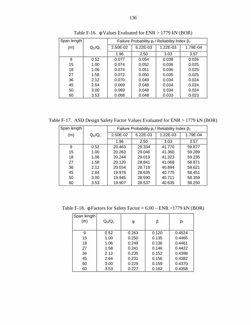
136
Table F-16. φ Values Evaluated for ENR > 1779 kN (BOR)
Span length Failure Probability pf / Reliability Index βΤ
(m) QD/QL 2.50E-02 6.22E-03 1.22E-03 1.79E-04
1.96 2.50 3.03 3.579 0.52 0.077 0.054 0.038 0.02615 1.00 0.074 0.052 0.036 0.02518 1.06 0.074 0.051 0.036 0.02527 1.58 0.072 0.050 0.035 0.02536 2.12 0.070 0.049 0.034 0.02445 2.64 0.069 0.048 0.034 0.02450 3.00 0.069 0.048 0.034 0.02460 3.53 0.068 0.048 0.033 0.023
Table F-17. ASD Design Safety Factor Values Evaluated for ENR > 1779 kN (BOR)
Span length Failure Probability pf / Reliability Index βΤ
(m) QD/QL 2.50E-02 6.22E-03 1.22E-03 1.79E-04
1.96 2.50 3.03 3.579 0.52 20.463 29.334 41.770 59.87715 1.00 20.263 29.046 41.360 59.28918 1.06 20.244 29.019 41.323 59.23527 1.58 20.120 28.841 41.068 58.87136 2.12 20.034 28.719 40.894 58.62145 2.64 19.976 28.635 40.775 58.45150 3.00 19.945 28.590 40.711 58.35960 3.53 19.907 28.537 40.635 58.250
Table F-18. φ Factors for Safety Factor = 6.00 – ENR >1779 kN (BOR)
Span length(m) QD/QL φ β pf
9 0.52 0.263 0.120 0.452415 1.00 0.250 0.135 0.446518 1.06 0.249 0.136 0.446127 1.58 0.241 0.146 0.442236 2.12 0.235 0.152 0.439845 2.64 0.231 0.156 0.438250 3.00 0.229 0.159 0.437060 3.53 0.227 0.162 0.4358

APPENDIX G
LRFD ANALYSIS RESULTS – MODIFIED ENR
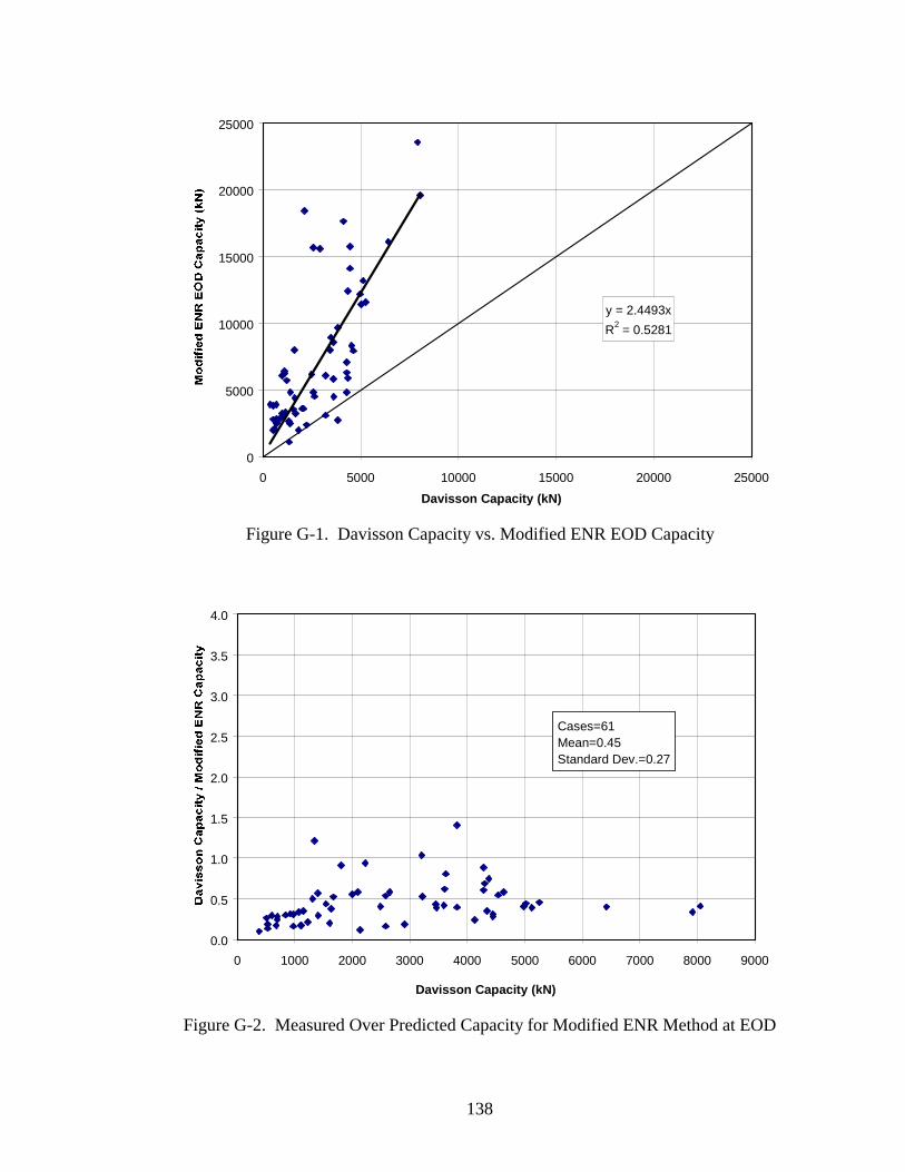
138
y = 2.4493x
R2 = 0.5281
0
5000
10000
15000
20000
25000
0 5000 10000 15000 20000 25000
Davisson Capacity (kN)
Figure G-1. Davisson Capacity vs. Modified ENR EOD Capacity
0.0
0.5
1.0
1.5
2.0
2.5
3.0
3.5
4.0
0 1000 2000 3000 4000 5000 6000 7000 8000 9000
Davisson Capacity (kN)
Cases=61Mean=0.45Standard Dev.=0.27
Figure G-2. Measured Over Predicted Capacity for Modified ENR Method at EOD

139
Table G-1. φ Values Evaluated for Modified ENR – Overall (EOD)
Span length Failure Probability pf / Reliability Index βΤ
(m) QD/QL 2.50E-02 6.22E-03 1.22E-03 1.79E-04
1.96 2.5 3.03 3.579 0.52 0.171 0.124 0.090 0.06515 1.00 0.164 0.119 0.087 0.06318 1.06 0.163 0.118 0.086 0.06327 1.58 0.159 0.115 0.084 0.06136 2.12 0.156 0.113 0.082 0.06045 2.64 0.154 0.111 0.081 0.05950 3.00 0.153 0.111 0.081 0.05960 3.53 0.151 0.110 0.080 0.058
Table G-2. ASD Design Safety Factor for Modified ENR – Overall (EOD)
Span length Failure Probability pf / Reliability Index βΤ
(m) QD/QL 2.50E-02 6.22E-03 1.22E-03 1.79E-04
1.96 2.5 3.03 3.579 0.52 9.241 12.747 17.480 24.11115 1.00 9.151 12.622 17.308 23.87518 1.06 9.142 12.611 17.292 23.85327 1.58 9.086 12.533 17.186 23.70636 2.12 9.047 12.480 17.113 23.60645 2.64 9.021 12.444 17.063 23.53750 3.00 9.007 12.424 17.036 23.50060 3.53 8.990 12.401 17.005 23.456
Table G-3. φ Factors for Safety Factor = 6.00 – Modified ENR – Overall (EOD)
Span length(m) QD/QL φ βΤ pf
9 0.52 0.263 1.235 0.108515 1.00 0.250 1.251 0.105618 1.06 0.249 1.253 0.105227 1.58 0.241 1.263 0.103436 2.12 0.235 1.270 0.102145 2.64 0.231 1.275 0.101250 3.00 0.229 1.278 0.100760 3.53 0.227 1.281 0.1002
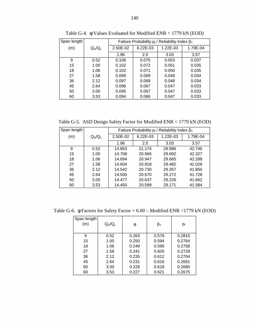
140
Table G-4. φ Values Evaluated for Modified ENR < 1779 kN (EOD)
Span length Failure Probability pf / Reliability Index βΤ
(m) QD/QL 2.50E-02 6.22E-03 1.22E-03 1.79E-04
1.96 2.5 3.03 3.579 0.52 0.106 0.075 0.053 0.03715 1.00 0.102 0.072 0.051 0.03518 1.06 0.102 0.071 0.050 0.03527 1.58 0.099 0.069 0.049 0.03436 2.12 0.097 0.068 0.048 0.03445 2.64 0.096 0.067 0.047 0.03350 3.00 0.095 0.067 0.047 0.03360 3.53 0.094 0.066 0.047 0.033
Table G-5. ASD Design Safety Factor for Modified ENR < 1779 kN (EOD)
Span length Failure Probability pf / Reliability Index βΤ
(m) QD/QL 2.50E-02 6.22E-03 1.22E-03 1.79E-04
1.96 2.5 3.03 3.579 0.52 14.853 21.174 29.986 42.74615 1.00 14.708 20.966 29.692 42.32718 1.06 14.694 20.947 29.665 42.28827 1.58 14.604 20.818 29.482 42.02836 2.12 14.542 20.730 29.357 41.85045 2.64 14.500 20.670 29.272 41.72850 3.00 14.477 20.637 29.226 41.66260 3.53 14.450 20.599 29.171 41.584
Table G-6. φ Factors for Safety Factor = 6.00 – Modified ENR <1779 kN (EOD)
Span length(m) QD/QL φ βΤ pf
9 0.52 0.263 0.579 0.281515 1.00 0.250 0.594 0.276418 1.06 0.249 0.596 0.275827 1.58 0.241 0.605 0.272836 2.12 0.235 0.612 0.270445 2.64 0.231 0.616 0.269150 3.00 0.229 0.618 0.268560 3.53 0.227 0.621 0.2675

141
Table G-7. φ Values Evaluated for Modified ENR > 1779 kN (EOD)
Span length Failure Probability pf / Reliability Index βΤ
(m) QD/QL 2.50E-02 6.22E-03 1.22E-03 1.79E-04
1.96 2.5 3.03 3.579 0.52 0.200 0.145 0.105 0.07615 1.00 0.192 0.139 0.101 0.07318 1.06 0.191 0.138 0.101 0.07327 1.58 0.186 0.135 0.098 0.07136 2.12 0.183 0.132 0.096 0.06945 2.64 0.180 0.130 0.095 0.06950 3.00 0.179 0.129 0.094 0.06860 3.53 0.177 0.128 0.093 0.067
Table G-8. ASD Design Safety Factor for Modified ENR > 1779 kN (EOD)
Span length Failure Probability pf / Reliability Index βΤ
(m) QD/QL 2.50E-02 6.22E-03 1.22E-03 1.79E-04
1.96 2.5 3.03 3.579 0.52 7.881 10.903 14.993 20.74215 1.00 7.804 10.796 14.846 20.53818 1.06 7.797 10.786 14.833 20.51927 1.58 7.749 10.720 14.741 20.39336 2.12 7.716 10.675 14.679 20.30745 2.64 7.694 10.644 14.636 20.24850 3.00 7.682 10.627 14.613 20.21660 3.53 7.667 10.607 14.586 20.178
Table G-9. φ Factors for Safety Factor = 6.00 – Modified ENR >1779 kN (EOD)
Span length(m) QD/QL φ βΤ pf
9 0.52 0.263 1.506 0.066115 1.00 0.250 1.523 0.063918 1.06 0.249 1.524 0.063827 1.58 0.241 1.534 0.062636 2.12 0.235 1.541 0.061745 2.64 0.231 1.546 0.061150 3.00 0.229 1.549 0.060860 3.53 0.227 1.552 0.0604
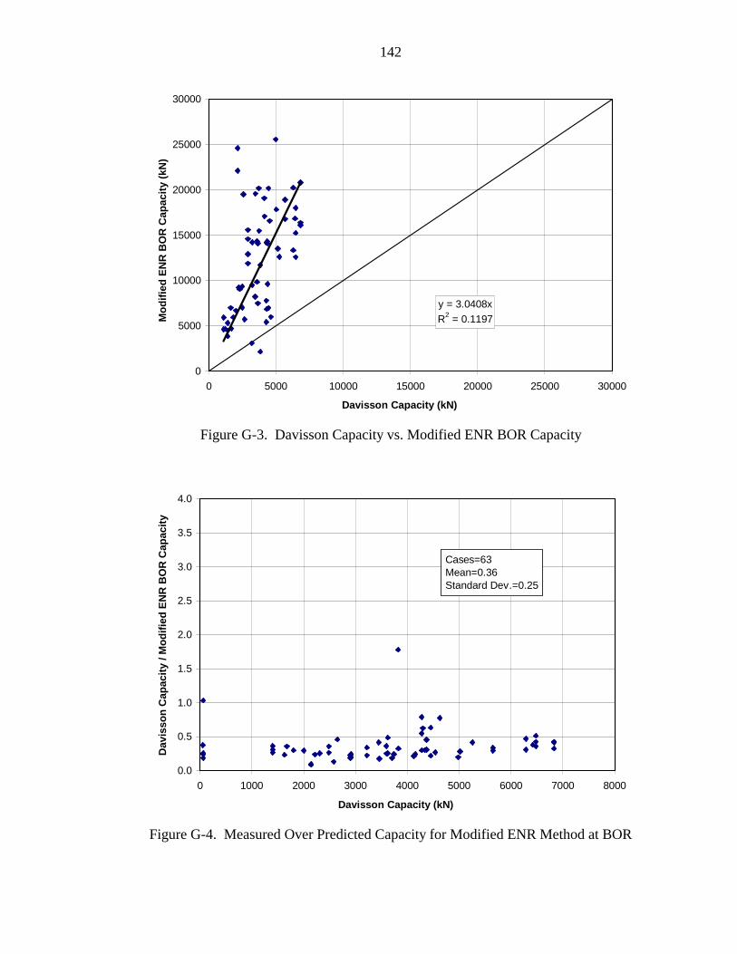
142
y = 3.0408xR2 = 0.1197
0
5000
10000
15000
20000
25000
30000
0 5000 10000 15000 20000 25000 30000
Davisson Capacity (kN)
Mod
ified
EN
R B
OR
Cap
acity
(kN
)
Figure G-3. Davisson Capacity vs. Modified ENR BOR Capacity
0.0
0.5
1.0
1.5
2.0
2.5
3.0
3.5
4.0
0 1000 2000 3000 4000 5000 6000 7000 8000
Davisson Capacity (kN)
Dav
isso
n C
apac
ity /
Mod
ified
EN
R B
OR
Cap
acity
Cases=63Mean=0.36Standard Dev.=0.25
Figure G-4. Measured Over Predicted Capacity for Modified ENR Method at BOR

143
Table G-10. φ Values Evaluated for Modified ENR – Overall (BOR)
Span length Failure Probability pf / Reliability Index βΤ
(m) QD/QL 2.50E-02 6.22E-03 1.22E-03 1.79E-04
1.96 2.50 3.03 3.579 0.52 0.121 0.085 0.060 0.04215 1.00 0.116 0.081 0.058 0.04018 1.06 0.115 0.081 0.057 0.04027 1.58 0.112 0.079 0.056 0.03936 2.12 0.110 0.077 0.055 0.03945 2.64 0.108 0.076 0.054 0.03850 3.00 0.108 0.076 0.054 0.03860 3.53 0.107 0.075 0.053 0.037
Table G-11. ASD Design Safety Factor for Modified ENR – Overall (BOR)
Span length Failure Probability pf / Reliability Index βΤ
(m) QD/QL 2.50E-02 6.22E-03 1.22E-03 1.79E-04
1.96 2.50 3.03 3.579 0.52 13.101 18.627 26.313 37.41315 1.00 12.972 18.445 26.055 37.04618 1.06 12.960 18.428 26.031 37.01227 1.58 12.881 18.314 25.871 36.78436 2.12 12.826 18.237 25.761 36.62845 2.64 12.789 18.184 25.686 36.52250 3.00 12.769 18.155 25.646 36.46460 3.53 12.745 18.121 25.598 36.396
Table G-12. φ Factors for Safety Factor = 6.00 – Modified ENR – Overall (BOR)
Span length(m) QD/QL φ β pf
9 0.52 0.263 0.762 0.223215 1.00 0.250 0.777 0.218718 1.06 0.249 0.778 0.218427 1.58 0.241 0.788 0.215536 2.12 0.235 0.794 0.213745 2.64 0.231 0.799 0.212350 3.00 0.229 0.801 0.211760 3.53 0.227 0.804 0.2108
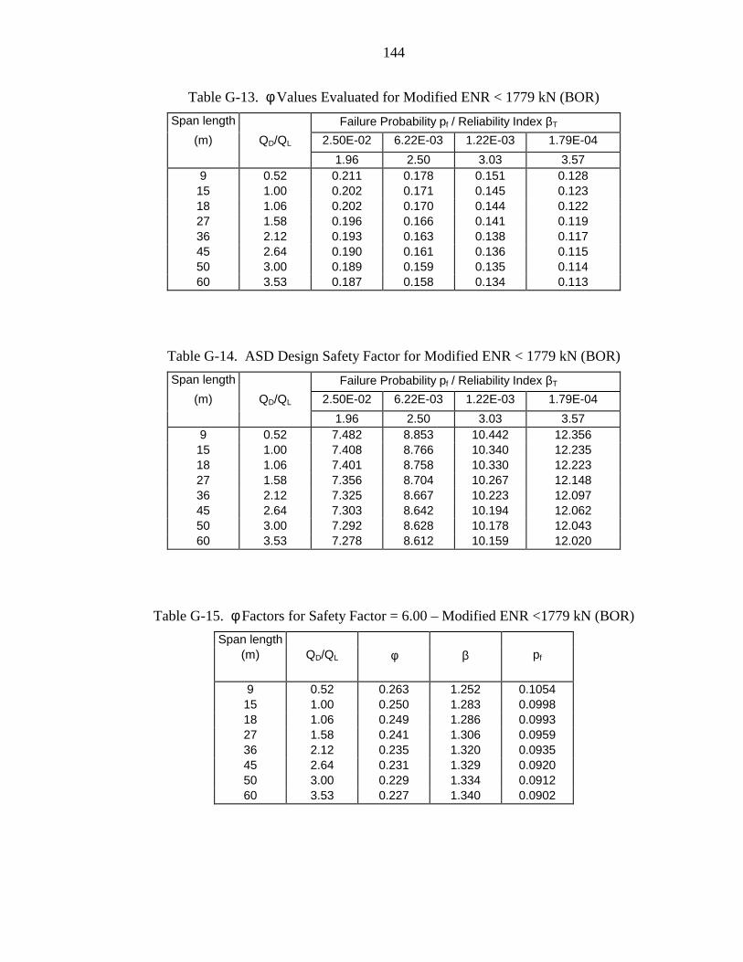
144
Table G-13. φ Values Evaluated for Modified ENR < 1779 kN (BOR)
Span length Failure Probability pf / Reliability Index βΤ
(m) QD/QL 2.50E-02 6.22E-03 1.22E-03 1.79E-04
1.96 2.50 3.03 3.579 0.52 0.211 0.178 0.151 0.12815 1.00 0.202 0.171 0.145 0.12318 1.06 0.202 0.170 0.144 0.12227 1.58 0.196 0.166 0.141 0.11936 2.12 0.193 0.163 0.138 0.11745 2.64 0.190 0.161 0.136 0.11550 3.00 0.189 0.159 0.135 0.11460 3.53 0.187 0.158 0.134 0.113
Table G-14. ASD Design Safety Factor for Modified ENR < 1779 kN (BOR)
Span length Failure Probability pf / Reliability Index βΤ
(m) QD/QL 2.50E-02 6.22E-03 1.22E-03 1.79E-04
1.96 2.50 3.03 3.579 0.52 7.482 8.853 10.442 12.35615 1.00 7.408 8.766 10.340 12.23518 1.06 7.401 8.758 10.330 12.22327 1.58 7.356 8.704 10.267 12.14836 2.12 7.325 8.667 10.223 12.09745 2.64 7.303 8.642 10.194 12.06250 3.00 7.292 8.628 10.178 12.04360 3.53 7.278 8.612 10.159 12.020
Table G-15. φ Factors for Safety Factor = 6.00 – Modified ENR <1779 kN (BOR)
Span length(m) QD/QL φ β pf
9 0.52 0.263 1.252 0.105415 1.00 0.250 1.283 0.099818 1.06 0.249 1.286 0.099327 1.58 0.241 1.306 0.095936 2.12 0.235 1.320 0.093545 2.64 0.231 1.329 0.092050 3.00 0.229 1.334 0.091260 3.53 0.227 1.340 0.0902
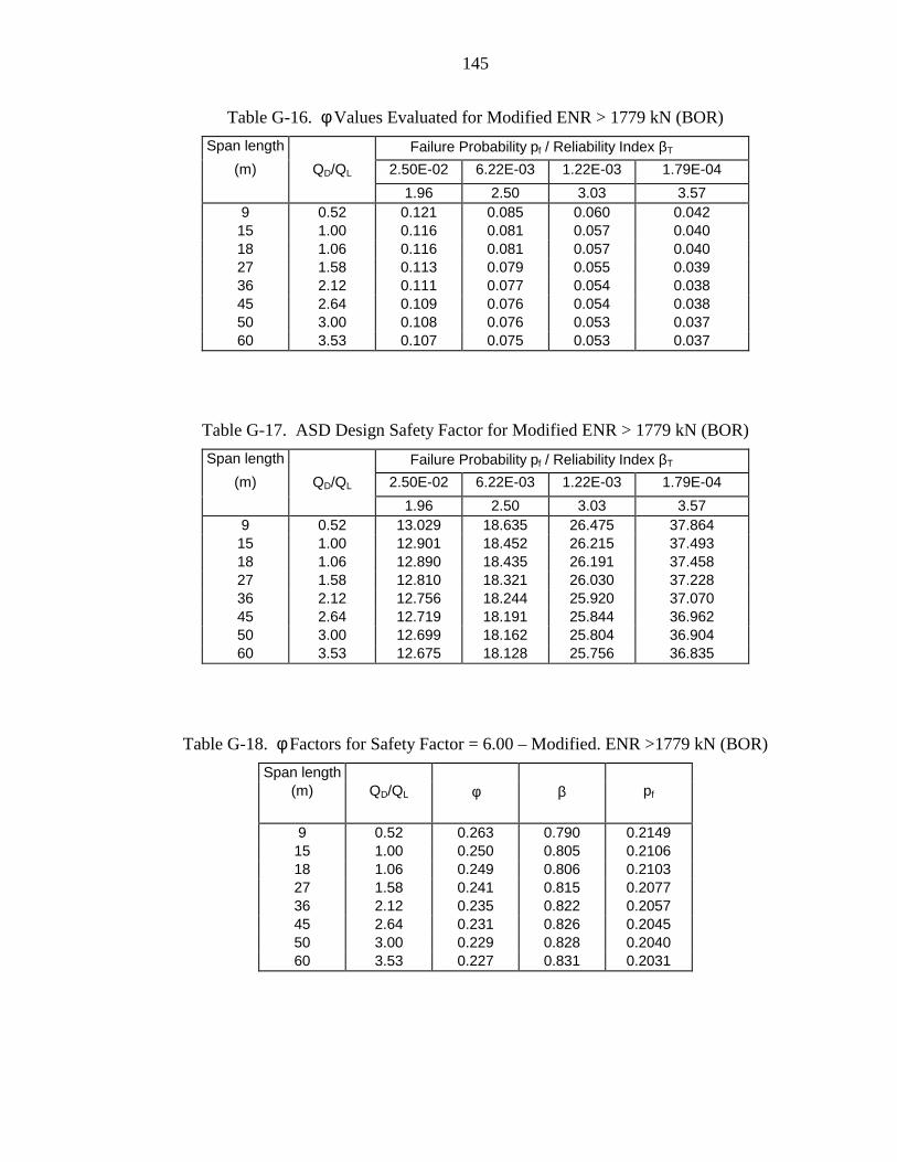
145
Table G-16. φ Values Evaluated for Modified ENR > 1779 kN (BOR)
Span length Failure Probability pf / Reliability Index βΤ
(m) QD/QL 2.50E-02 6.22E-03 1.22E-03 1.79E-04
1.96 2.50 3.03 3.579 0.52 0.121 0.085 0.060 0.04215 1.00 0.116 0.081 0.057 0.04018 1.06 0.116 0.081 0.057 0.04027 1.58 0.113 0.079 0.055 0.03936 2.12 0.111 0.077 0.054 0.03845 2.64 0.109 0.076 0.054 0.03850 3.00 0.108 0.076 0.053 0.03760 3.53 0.107 0.075 0.053 0.037
Table G-17. ASD Design Safety Factor for Modified ENR > 1779 kN (BOR)
Span length Failure Probability pf / Reliability Index βΤ
(m) QD/QL 2.50E-02 6.22E-03 1.22E-03 1.79E-04
1.96 2.50 3.03 3.579 0.52 13.029 18.635 26.475 37.86415 1.00 12.901 18.452 26.215 37.49318 1.06 12.890 18.435 26.191 37.45827 1.58 12.810 18.321 26.030 37.22836 2.12 12.756 18.244 25.920 37.07045 2.64 12.719 18.191 25.844 36.96250 3.00 12.699 18.162 25.804 36.90460 3.53 12.675 18.128 25.756 36.835
Table G-18. φ Factors for Safety Factor = 6.00 – Modified. ENR >1779 kN (BOR)
Span length(m) QD/QL φ β pf
9 0.52 0.263 0.790 0.214915 1.00 0.250 0.805 0.210618 1.06 0.249 0.806 0.210327 1.58 0.241 0.815 0.207736 2.12 0.235 0.822 0.205745 2.64 0.231 0.826 0.204550 3.00 0.229 0.828 0.204060 3.53 0.227 0.831 0.2031

APPENDIX H
LRFD ANALYSIS RESULTS – GATES FORMULA
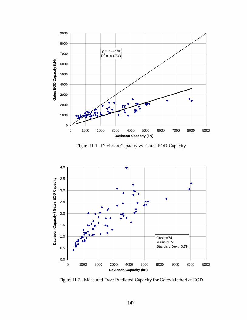
147
y = 0.4487xR2 = -0.0733
0
1000
2000
3000
4000
5000
6000
7000
8000
9000
0 1000 2000 3000 4000 5000 6000 7000 8000 9000
Davisson Capacity (kN)
Gat
es E
OD
Cap
acity
(kN
)
Figure H-1. Davisson Capacity vs. Gates EOD Capacity
0.0
0.5
1.0
1.5
2.0
2.5
3.0
3.5
4.0
0 1000 2000 3000 4000 5000 6000 7000 8000 9000
Davisson Capacity (kN)
Dav
isso
n C
apac
ity /
Gat
es E
OD
Cap
acity
Cases=74Mean=1.74Standard Dev.=0.79
Figure H-2. Measured Over Predicted Capacity for Gates Method at EOD

148
Table H-1. φ Values Evaluated for Gates – Overall (EOD)
Span length Failure Probability pf / Reliability Index βΤ
(m) QD/QL 2.50E-02 6.22E-03 1.22E-03 1.79E-04
1.96 2.5 3.03 3.579 0.52 0.884 0.681 0.527 0.40615 1.00 0.848 0.653 0.505 0.38918 1.06 0.845 0.651 0.503 0.38827 1.58 0.822 0.633 0.490 0.37736 2.12 0.806 0.621 0.481 0.37045 2.64 0.796 0.613 0.474 0.36550 3.00 0.790 0.608 0.471 0.36360 3.53 0.783 0.603 0.467 0.359
Table H-2. ASD Design Safety Factor for Gates – Overall (EOD)
Span length Failure Probability pf / Reliability Index βΤ
(m) QD/QL 2.50E-02 6.22E-03 1.22E-03 1.79E-04
1.96 2.5 3.03 3.579 0.52 1.786 2.319 2.997 3.89115 1.00 1.769 2.297 2.967 3.85318 1.06 1.767 2.294 2.965 3.84927 1.58 1.756 2.280 2.946 3.82636 2.12 1.749 2.271 2.934 3.80945 2.64 1.744 2.264 2.925 3.79850 3.00 1.741 2.260 2.921 3.79260 3.53 1.738 2.256 2.915 3.785
Table H-3. φ Factors for Safety Factor = 3.00 – Gates – Overall (EOD)
Span length(m) QD/QL φ βΤ pf
9 0.52 0.526 3.032 0.0012215 1.00 0.500 3.053 0.0011318 1.06 0.498 3.054 0.0011327 1.58 0.481 3.067 0.0010836 2.12 0.470 3.076 0.0010545 2.64 0.462 3.082 0.0010350 3.00 0.458 3.085 0.0010260 3.53 0.453 3.089 0.00101

149
Table H-4. φ Values Evaluated for Gates < 1779 kN (EOD)
Span length Failure Probability pf / Reliability Index βΤ
(m) QD/QL 2.50E-02 6.22E-03 1.22E-03 1.79E-04
1.96 2.5 3.03 3.579 0.52 0.683 0.554 0.451 0.36615 1.00 0.655 0.532 0.433 0.35118 1.06 0.653 0.529 0.431 0.35027 1.58 0.635 0.515 0.420 0.34036 2.12 0.623 0.505 0.412 0.33445 2.64 0.615 0.499 0.406 0.32950 3.00 0.610 0.495 0.403 0.32760 3.53 0.605 0.491 0.400 0.324
Table H-5. ASD Design Safety Factor for Gates < 1779 kN (EOD)
Span length Failure Probability pf / Reliability Index βΤ
(m) QD/QL 2.50E-02 6.22E-03 1.22E-03 1.79E-04
1.96 2.5 3.03 3.579 0.52 2.311 2.850 3.500 4.31615 1.00 2.289 2.822 3.466 4.27318 1.06 2.286 2.819 3.463 4.26927 1.58 2.272 2.802 3.441 4.24336 2.12 2.263 2.790 3.427 4.22545 2.64 2.256 2.782 3.417 4.21350 3.00 2.253 2.777 3.411 4.20660 3.53 2.248 2.772 3.405 4.198
Table H-6. φ Factors for Safety Factor = 3.00 – Gates <1779 kN (EOD)
Span length(m) QD/QL φ βΤ pf
9 0.52 0.526 2.632 0.0042515 1.00 0.500 2.658 0.0039418 1.06 0.498 2.660 0.0039127 1.58 0.481 2.676 0.0037336 2.12 0.470 2.687 0.0036145 2.64 0.462 2.695 0.0035250 3.00 0.458 2.699 0.0034860 3.53 0.453 2.704 0.00343
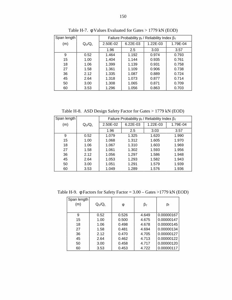
150
Table H-7. φ Values Evaluated for Gates > 1779 kN (EOD)
Span length Failure Probability pf / Reliability Index βΤ
(m) QD/QL 2.50E-02 6.22E-03 1.22E-03 1.79E-04
1.96 2.5 3.03 3.579 0.52 1.464 1.192 0.974 0.79315 1.00 1.404 1.144 0.935 0.76118 1.06 1.399 1.139 0.931 0.75827 1.58 1.361 1.109 0.906 0.73836 2.12 1.335 1.087 0.889 0.72445 2.64 1.318 1.073 0.877 0.71450 3.00 1.308 1.065 0.871 0.70960 3.53 1.296 1.056 0.863 0.703
Table H-8. ASD Design Safety Factor for Gates > 1779 kN (EOD)
Span length Failure Probability pf / Reliability Index βΤ
(m) QD/QL 2.50E-02 6.22E-03 1.22E-03 1.79E-04
1.96 2.5 3.03 3.579 0.52 1.079 1.325 1.620 1.99015 1.00 1.068 1.312 1.605 1.97018 1.06 1.067 1.310 1.603 1.96927 1.58 1.061 1.302 1.593 1.95636 2.12 1.056 1.297 1.586 1.94845 2.64 1.053 1.293 1.582 1.94350 3.00 1.051 1.291 1.579 1.93960 3.53 1.049 1.289 1.576 1.936
Table H-9. φ Factors for Safety Factor = 3.00 – Gates >1779 kN (EOD)
Span length(m) QD/QL φ βΤ pf
9 0.52 0.526 4.649 0.0000016715 1.00 0.500 4.675 0.0000014718 1.06 0.498 4.678 0.0000014527 1.58 0.481 4.694 0.0000013436 2.12 0.470 4.705 0.0000012745 2.64 0.462 4.713 0.0000012250 3.00 0.458 4.717 0.0000012060 3.53 0.453 4.722 0.00000117
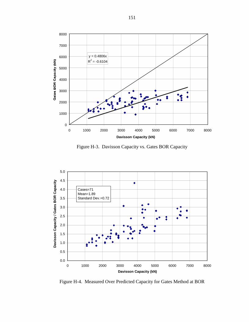
151
y = 0.4806x
R2 = -0.6104
0
1000
2000
3000
4000
5000
6000
7000
8000
0 1000 2000 3000 4000 5000 6000 7000 8000
Davisson Capacity (kN)
Figure H-3. Davisson Capacity vs. Gates BOR Capacity
0.0
0.5
1.0
1.5
2.0
2.5
3.0
3.5
4.0
4.5
5.0
0 1000 2000 3000 4000 5000 6000 7000 8000
Davisson Capacity (kN)
Dav
isso
n C
apac
ity /
Gat
es B
OR
Cap
acity
Cases=71Mean=1.89Standard Dev.=0.72
Figure H-4. Measured Over Predicted Capacity for Gates Method at BOR

152
Table H-10. φ Values Evaluated for Gates – Overall (BOR)
Span length Failure Probability pf / Reliability Index βΤ
(m) QD/QL 2.50E-02 6.22E-03 1.22E-03 1.79E-04
1.96 2.50 3.03 3.579 0.52 1.097 0.871 0.694 0.55115 1.00 1.052 0.835 0.666 0.52918 1.06 1.048 0.832 0.664 0.52727 1.58 1.020 0.810 0.646 0.51336 2.12 1.000 0.794 0.633 0.50345 2.64 0.987 0.784 0.625 0.49650 3.00 0.980 0.778 0.620 0.49360 3.53 0.971 0.771 0.615 0.488
Table H-11. ASD Design Safety Factor for Gates – Overall (BOR)
Span length Failure Probability pf / Reliability Index βΤ
(m) QD/QL 2.50E-02 6.22E-03 1.22E-03 1.79E-04
1.96 2.50 3.03 3.579 0.52 1.440 1.813 2.274 2.86415 1.00 1.426 1.796 2.252 2.83618 1.06 1.424 1.794 2.250 2.83327 1.58 1.416 1.783 2.236 2.81636 2.12 1.410 1.775 2.226 2.80445 2.64 1.406 1.770 2.220 2.79650 3.00 1.403 1.767 2.216 2.79160 3.53 1.401 1.764 2.212 2.786
Table H-12. φ Factors for Safety Factor = 3.00 – Gates – Overall (BOR)
Span length(m) QD/QL φ β pf
9 0.52 0.526 3.679 0.000117315 1.00 0.500 3.702 0.000107218 1.06 0.498 3.704 0.000106327 1.58 0.481 3.718 0.000100636 2.12 0.470 3.728 0.000096745 2.64 0.462 3.735 0.000094050 3.00 0.458 3.739 0.000092660 3.53 0.453 3.743 0.0000911

153
Table H-13. φ Values Evaluated for Gates < 1779 kN (BOR)
Span length Failure Probability pf / Reliability Index βΤ
(m) QD/QL 2.50E-02 6.22E-03 1.22E-03 1.79E-04
1.96 2.50 3.03 3.579 0.52 0.855 0.732 0.628 0.53815 1.00 0.821 0.702 0.603 0.51618 1.06 0.817 0.700 0.600 0.51427 1.58 0.796 0.681 0.584 0.50036 2.12 0.780 0.668 0.573 0.49145 2.64 0.770 0.659 0.566 0.48450 3.00 0.764 0.654 0.561 0.48060 3.53 0.758 0.648 0.556 0.476
Table H-14. ASD Design Safety Factor for Gates < 1779 kN (BOR)
Span length Failure Probability pf / Reliability Index βΤ
(m) QD/QL 2.50E-02 6.22E-03 1.22E-03 1.79E-04
1.96 2.50 3.03 3.579 0.52 1.846 2.157 2.513 2.93615 1.00 1.828 2.136 2.488 2.90818 1.06 1.826 2.134 2.486 2.90527 1.58 1.815 2.121 2.471 2.88736 2.12 1.807 2.112 2.460 2.87545 2.64 1.802 2.105 2.453 2.86650 3.00 1.799 2.102 2.449 2.86260 3.53 1.796 2.098 2.445 2.857
Table H-15. φ Factors for Safety Factor = 3.00 – Gates <1779 kN (BOR)
Span length(m) QD/QL φ β pf
9 0.52 0.526 3.644 0.000134515 1.00 0.500 3.679 0.000117318 1.06 0.498 3.682 0.000115927 1.58 0.481 3.703 0.000106736 2.12 0.470 3.718 0.000100645 2.64 0.462 3.728 0.000096750 3.00 0.458 3.733 0.000094860 3.53 0.453 3.740 0.0000922
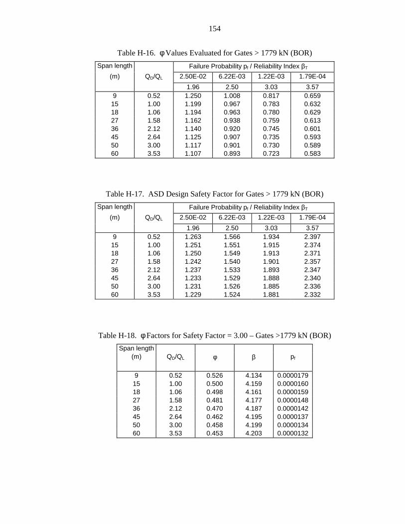
154
Table H-16. φ Values Evaluated for Gates > 1779 kN (BOR)
Span length Failure Probability pf / Reliability Index βΤ
(m) QD/QL 2.50E-02 6.22E-03 1.22E-03 1.79E-04
1.96 2.50 3.03 3.579 0.52 1.250 1.008 0.817 0.65915 1.00 1.199 0.967 0.783 0.63218 1.06 1.194 0.963 0.780 0.62927 1.58 1.162 0.938 0.759 0.61336 2.12 1.140 0.920 0.745 0.60145 2.64 1.125 0.907 0.735 0.59350 3.00 1.117 0.901 0.730 0.58960 3.53 1.107 0.893 0.723 0.583
Table H-17. ASD Design Safety Factor for Gates > 1779 kN (BOR)
Span length Failure Probability pf / Reliability Index βΤ
(m) QD/QL 2.50E-02 6.22E-03 1.22E-03 1.79E-04
1.96 2.50 3.03 3.579 0.52 1.263 1.566 1.934 2.39715 1.00 1.251 1.551 1.915 2.37418 1.06 1.250 1.549 1.913 2.37127 1.58 1.242 1.540 1.901 2.35736 2.12 1.237 1.533 1.893 2.34745 2.64 1.233 1.529 1.888 2.34050 3.00 1.231 1.526 1.885 2.33660 3.53 1.229 1.524 1.881 2.332
Table H-18. φ Factors for Safety Factor = 3.00 – Gates >1779 kN (BOR)
Span length(m) QD/QL φ β pf
9 0.52 0.526 4.134 0.000017915 1.00 0.500 4.159 0.000016018 1.06 0.498 4.161 0.000015927 1.58 0.481 4.177 0.000014836 2.12 0.470 4.187 0.000014245 2.64 0.462 4.195 0.000013750 3.00 0.458 4.199 0.000013460 3.53 0.453 4.203 0.0000132

APPENDIX I
FORCE AND VELOCITY TRACES FROM PDA SIGNAL
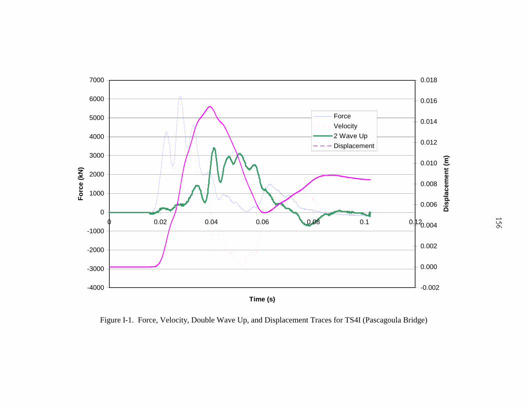
-4000
-3000
-2000
-1000
0
1000
2000
3000
4000
5000
6000
7000
0 0.02 0.04 0.06 0.08 0.1 0.12
Time (s)
For
ce (
kN)
-0.002
0.000
0.002
0.004
0.006
0.008
0.010
0.012
0.014
0.016
0.018
Dis
plac
emen
t (m
)
Force
Velocity
2 Wave Up
Displacement
Figure I-1. Force, Velocity, Double Wave Up, and Displacement Traces for TS4I (Pascagoula Bridge)
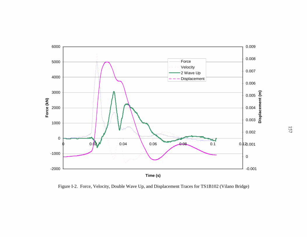
-2000
-1000
0
1000
2000
3000
4000
5000
6000
0 0.02 0.04 0.06 0.08 0.1 0.12
Time (s)
For
ce (
kN)
-0.001
0
0.001
0.002
0.003
0.004
0.005
0.006
0.007
0.008
0.009
Dis
plac
emen
t (m
)
Force
Velocity
2 Wave Up
Displacement
Figure I-2. Force, Velocity, Double Wave Up, and Displacement Traces for TS1B102 (Vilano Bridge)
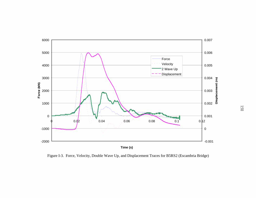
-2000
-1000
0
1000
2000
3000
4000
5000
6000
0 0.02 0.04 0.06 0.08 0.1 0.12
Time (s)
-0.001
0
0.001
0.002
0.003
0.004
0.005
0.006
0.007
Force
Velocity
2 Wave Up
Displacement
Figure I-3. Force, Velocity, Double Wave Up, and Displacement Traces for B5RS2 (Escambria Bridge)
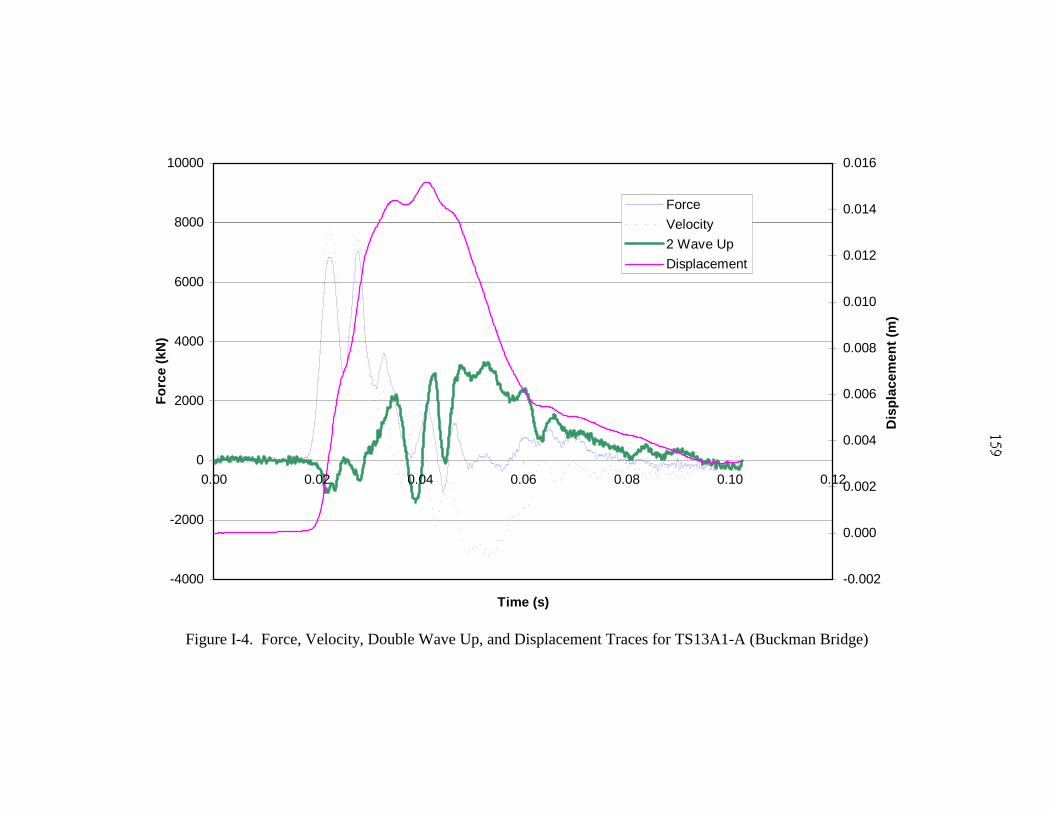
-4000
-2000
0
2000
4000
6000
8000
10000
0.00 0.02 0.04 0.06 0.08 0.10 0.12
Time (s)
For
ce (
kN)
-0.002
0.000
0.002
0.004
0.006
0.008
0.010
0.012
0.014
0.016
Dis
plac
emen
t (m
)
Force
Velocity
2 Wave Up
Displacement
Figure I-4. Force, Velocity, Double Wave Up, and Displacement Traces for TS13A1-A (Buckman Bridge)
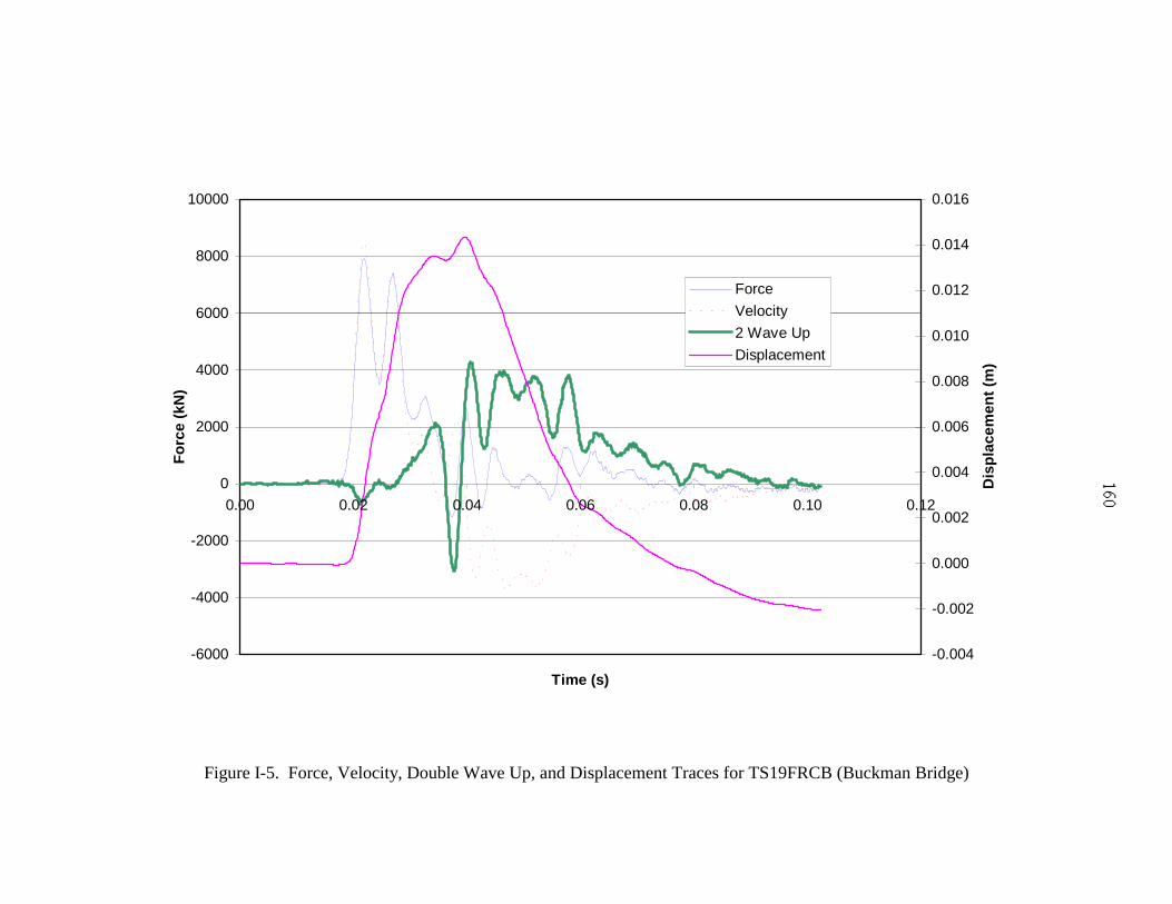
-6000
-4000
-2000
0
2000
4000
6000
8000
10000
0.00 0.02 0.04 0.06 0.08 0.10 0.12
Time (s)
For
ce (
kN)
-0.004
-0.002
0.000
0.002
0.004
0.006
0.008
0.010
0.012
0.014
0.016
Dis
plac
emen
t (m
)
Force
Velocity
2 Wave Up
Displacement
Figure I-5. Force, Velocity, Double Wave Up, and Displacement Traces for TS19FRCB (Buckman Bridge)
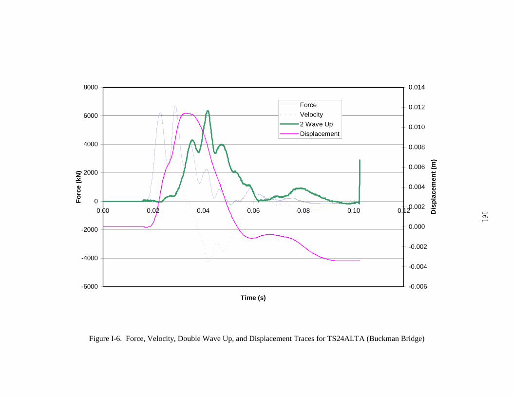
-6000
-4000
-2000
0
2000
4000
6000
8000
0.00 0.02 0.04 0.06 0.08 0.10 0.12
Time (s)
For
ce (
kN)
-0.006
-0.004
-0.002
0.000
0.002
0.004
0.006
0.008
0.010
0.012
0.014
Dis
plac
emen
t (m
)
Force
Velocity
2 Wave Up
Displacement
Figure I-6. Force, Velocity, Double Wave Up, and Displacement Traces for TS24ALTA (Buckman Bridge)
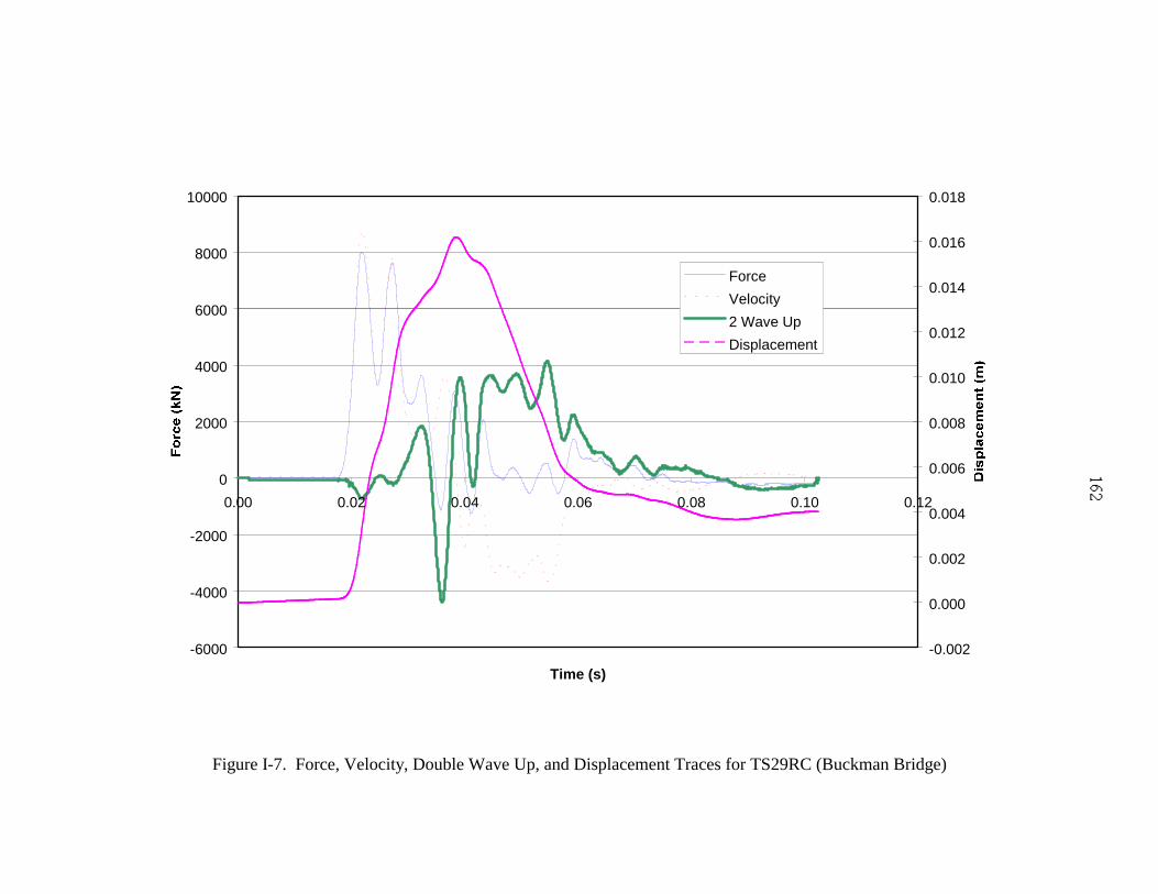
-6000
-4000
-2000
0
2000
4000
6000
8000
10000
0.00 0.02 0.04 0.06 0.08 0.10 0.12
Time (s)
-0.002
0.000
0.002
0.004
0.006
0.008
0.010
0.012
0.014
0.016
0.018
Force
Velocity
2 Wave Up
Displacement
Figure I-7. Force, Velocity, Double Wave Up, and Displacement Traces for TS29RC (Buckman Bridge)
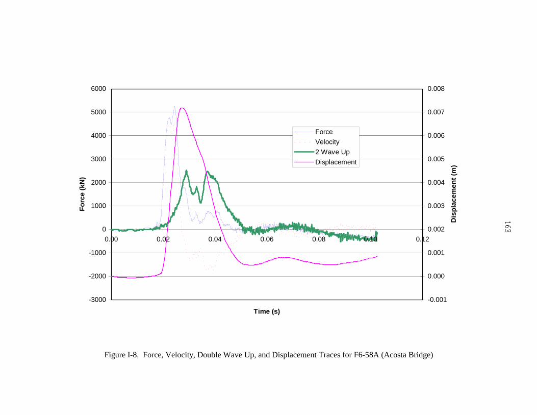
-3000
-2000
-1000
0
1000
2000
3000
4000
5000
6000
0.00 0.02 0.04 0.06 0.08 0.10 0.12
Time (s)
For
ce (
kN)
-0.001
0.000
0.001
0.002
0.003
0.004
0.005
0.006
0.007
0.008
Dis
plac
emen
t (m
)
Force
Velocity
2 Wave Up
Displacement
Figure I-8. Force, Velocity, Double Wave Up, and Displacement Traces for F6-58A (Acosta Bridge)
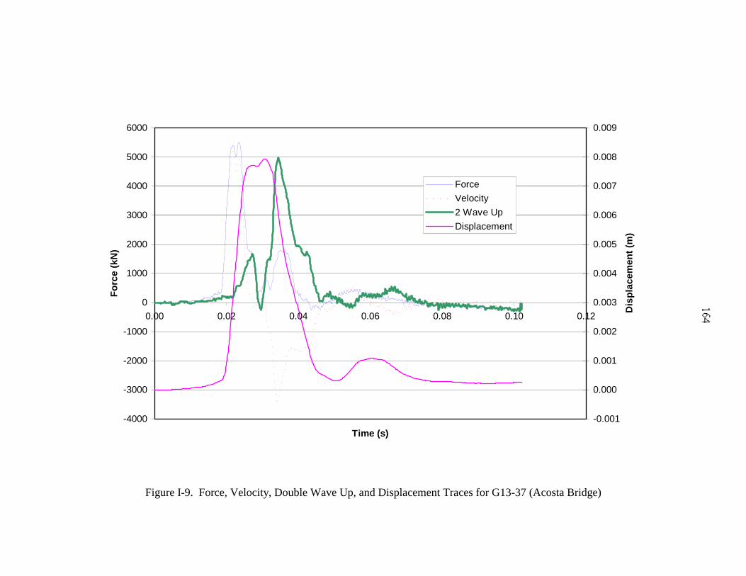
-4000
-3000
-2000
-1000
0
1000
2000
3000
4000
5000
6000
0.00 0.02 0.04 0.06 0.08 0.10 0.12
Time (s)
For
ce (
kN)
-0.001
0.000
0.001
0.002
0.003
0.004
0.005
0.006
0.007
0.008
0.009
Dis
plac
emen
t (m
)
Force
Velocity
2 Wave Up
Displacement
Figure I-9. Force, Velocity, Double Wave Up, and Displacement Traces for G13-37 (Acosta Bridge)

-5000
-4000
-3000
-2000
-1000
0
1000
2000
3000
4000
5000
6000
0.00 0.02 0.04 0.06 0.08 0.10 0.12
Time (s)
For
ce (
kN)
-0.002
0.000
0.002
0.004
0.006
0.008
0.010
0.012
Dis
plac
emen
t (m
)
Force
Velocity
2 Wave Up
Displacement
Figure I-10. Force, Velocity, Double Wave Up, and Displacement Traces for H2-27B (Acosta Bridge)
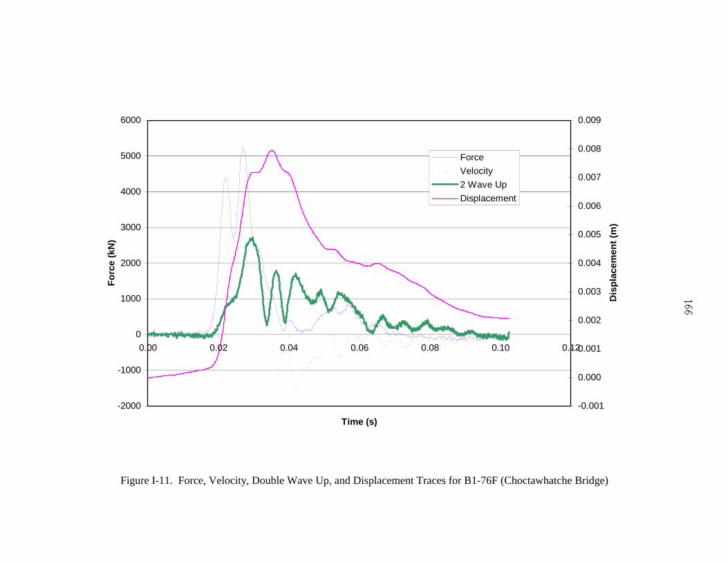
-2000
-1000
0
1000
2000
3000
4000
5000
6000
0.00 0.02 0.04 0.06 0.08 0.10 0.12
Time (s)
For
ce (
kN)
-0.001
0.000
0.001
0.002
0.003
0.004
0.005
0.006
0.007
0.008
0.009
Dis
plac
emen
t (m
)
Force
Velocity
2 Wave Up
Displacement
Figure I-11. Force, Velocity, Double Wave Up, and Displacement Traces for B1-76F (Choctawhatche Bridge)
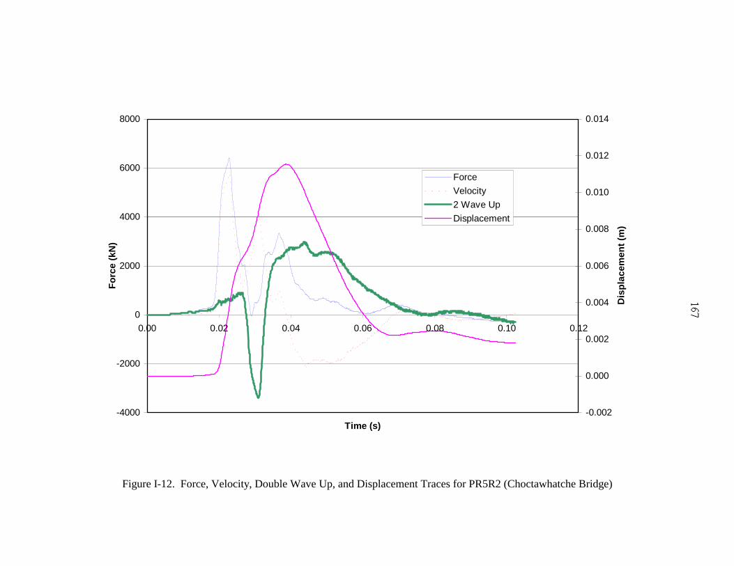
-4000
-2000
0
2000
4000
6000
8000
0.00 0.02 0.04 0.06 0.08 0.10 0.12
Time (s)
For
ce (
kN)
-0.002
0.000
0.002
0.004
0.006
0.008
0.010
0.012
0.014
Dis
plac
emen
t (m
)
Force
Velocity
2 Wave Up
Displacement
Figure I-12. Force, Velocity, Double Wave Up, and Displacement Traces for PR5R2 (Choctawhatche Bridge)
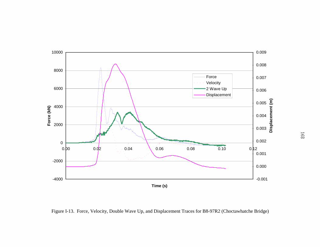
-4000
-2000
0
2000
4000
6000
8000
10000
0.00 0.02 0.04 0.06 0.08 0.10 0.12
Time (s)
For
ce (
kN)
-0.001
0.000
0.001
0.002
0.003
0.004
0.005
0.006
0.007
0.008
0.009
Dis
plac
emen
t (m
)
Force
Velocity
2 Wave Up
Displacement
Figure I-13. Force, Velocity, Double Wave Up, and Displacement Traces for B8-97R2 (Choctawhatche Bridge)
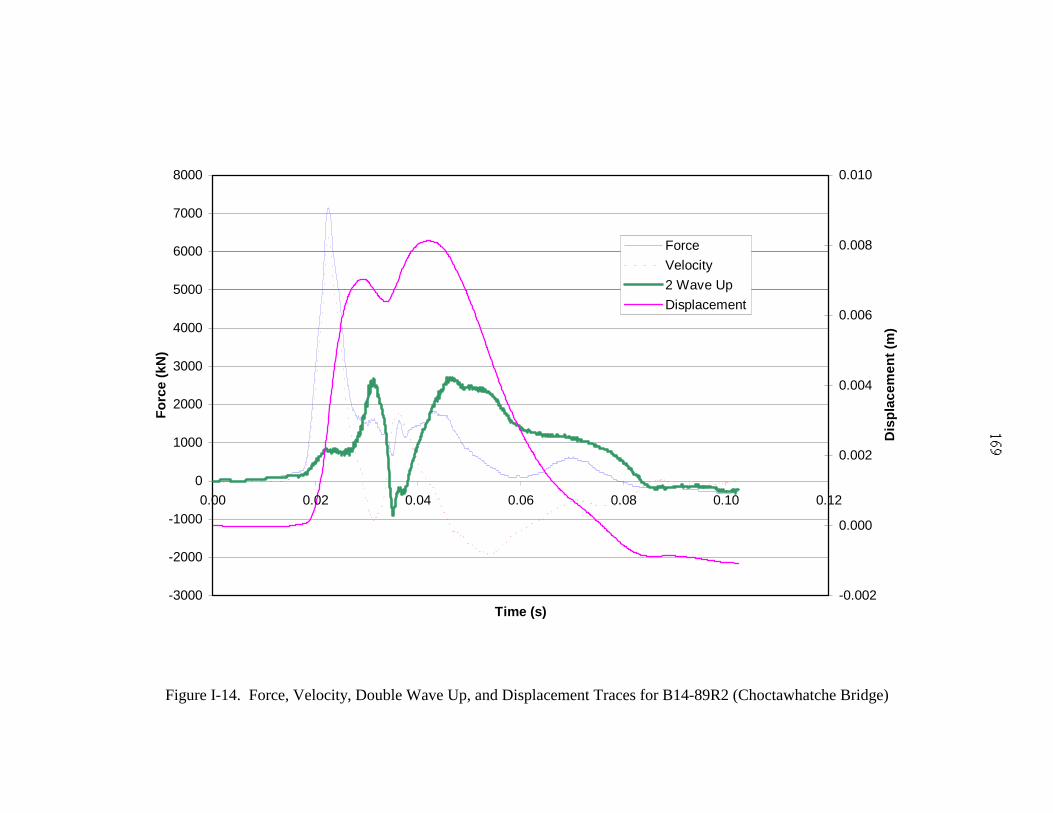
-3000
-2000
-1000
0
1000
2000
3000
4000
5000
6000
7000
8000
0.00 0.02 0.04 0.06 0.08 0.10 0.12
Time (s)
For
ce (
kN)
-0.002
0.000
0.002
0.004
0.006
0.008
0.010
Dis
plac
emen
t (m
)
Force
Velocity
2 Wave Up
Displacement
Figure I-14. Force, Velocity, Double Wave Up, and Displacement Traces for B14-89R2 (Choctawhatche Bridge)
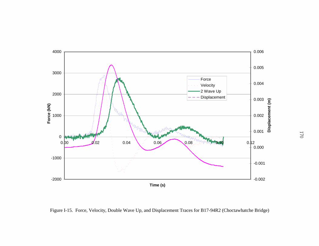
-2000
-1000
0
1000
2000
3000
4000
0.00 0.02 0.04 0.06 0.08 0.10 0.12
Time (s)
For
ce (
kN)
-0.002
-0.001
0.000
0.001
0.002
0.003
0.004
0.005
0.006
Dis
plac
emen
t (m
)
Force
Velocity
2 Wave Up
Displacement
Figure I-15. Force, Velocity, Double Wave Up, and Displacement Traces for B17-94R2 (Choctawhatche Bridge)
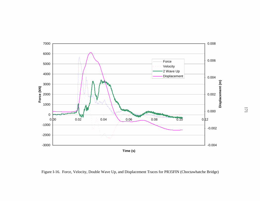
-3000
-2000
-1000
0
1000
2000
3000
4000
5000
6000
7000
0.00 0.02 0.04 0.06 0.08 0.10 0.12
Time (s)
For
ce (
kN)
-0.004
-0.002
0.000
0.002
0.004
0.006
0.008
Dis
plac
emen
t (m
)
Force
Velocity
2 Wave Up
Displacement
Figure I-16. Force, Velocity, Double Wave Up, and Displacement Traces for PR35FIN (Choctawhatche Bridge)
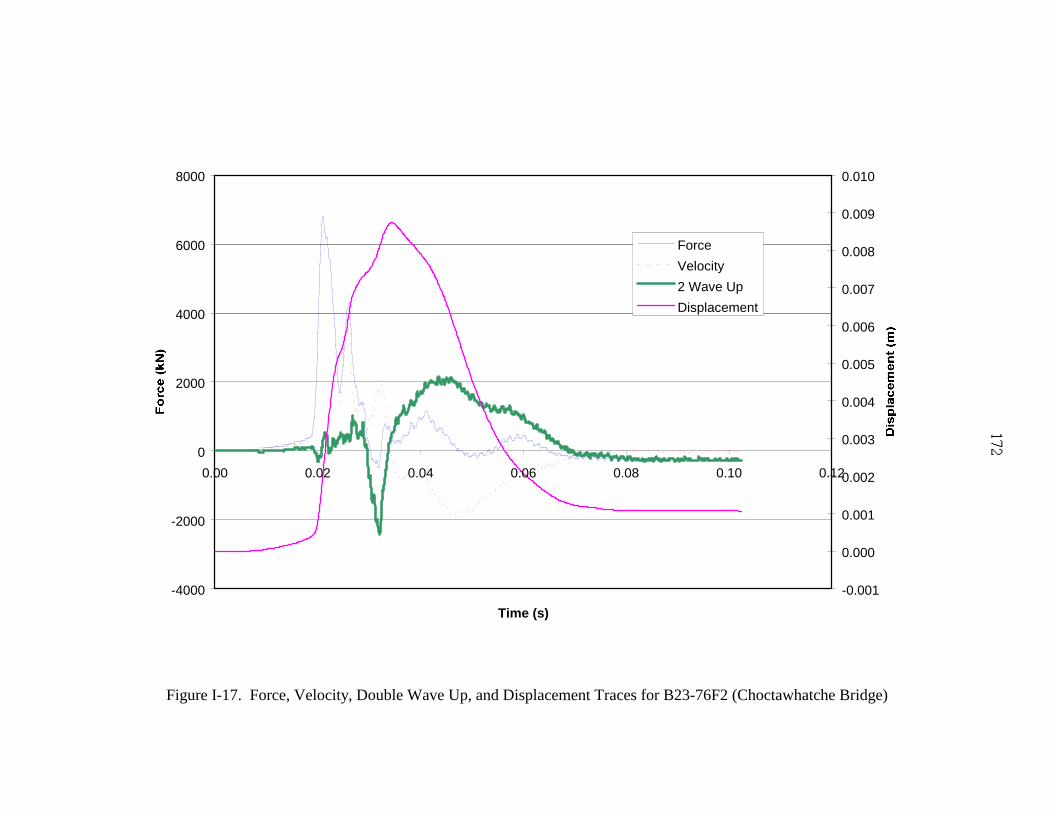
-4000
-2000
0
2000
4000
6000
8000
0.00 0.02 0.04 0.06 0.08 0.10 0.12
Time (s)
-0.001
0.000
0.001
0.002
0.003
0.004
0.005
0.006
0.007
0.008
0.009
0.010
Force
Velocity
2 Wave Up
Displacement
Figure I-17. Force, Velocity, Double Wave Up, and Displacement Traces for B23-76F2 (Choctawhatche Bridge)
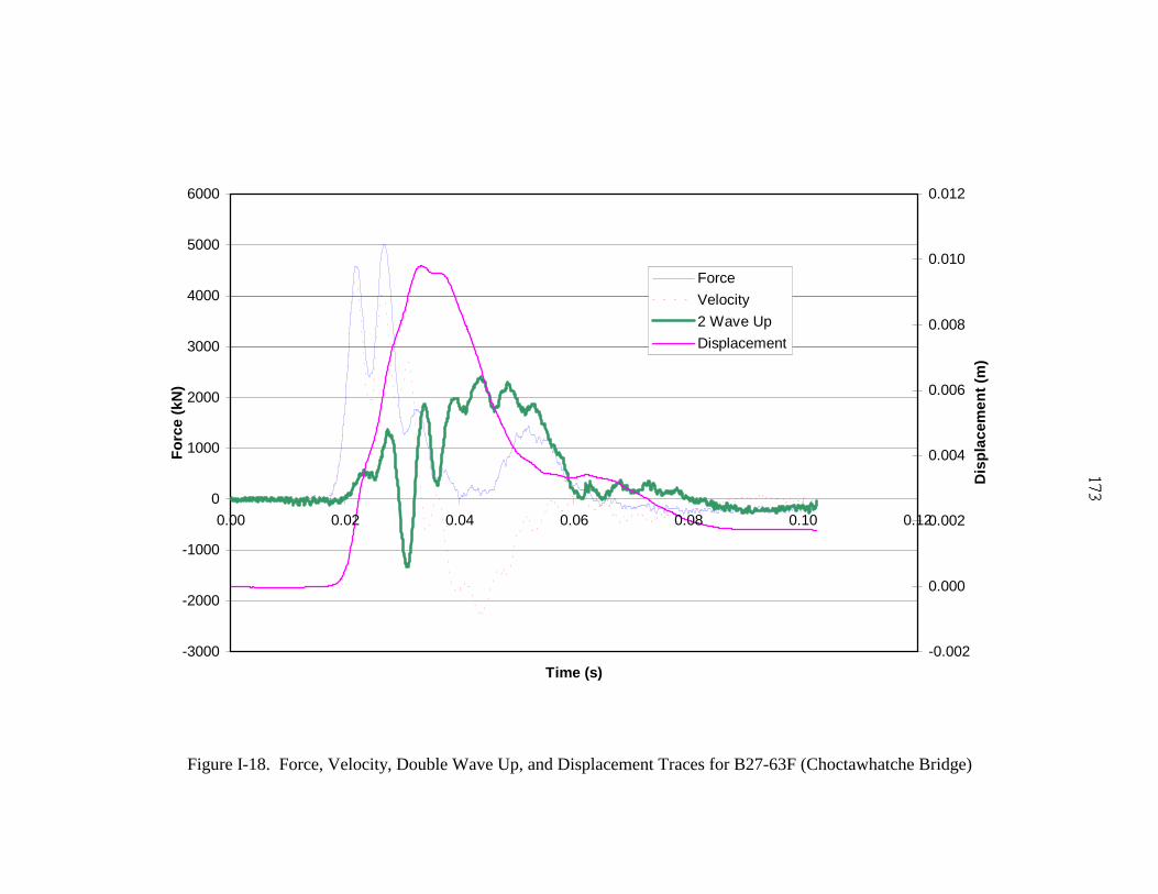
-3000
-2000
-1000
0
1000
2000
3000
4000
5000
6000
0.00 0.02 0.04 0.06 0.08 0.10 0.12
Time (s)
For
ce (
kN)
-0.002
0.000
0.002
0.004
0.006
0.008
0.010
0.012
Dis
plac
emen
t (m
)
Force
Velocity
2 Wave Up
Displacement
Figure I-18. Force, Velocity, Double Wave Up, and Displacement Traces for B27-63F (Choctawhatche Bridge)
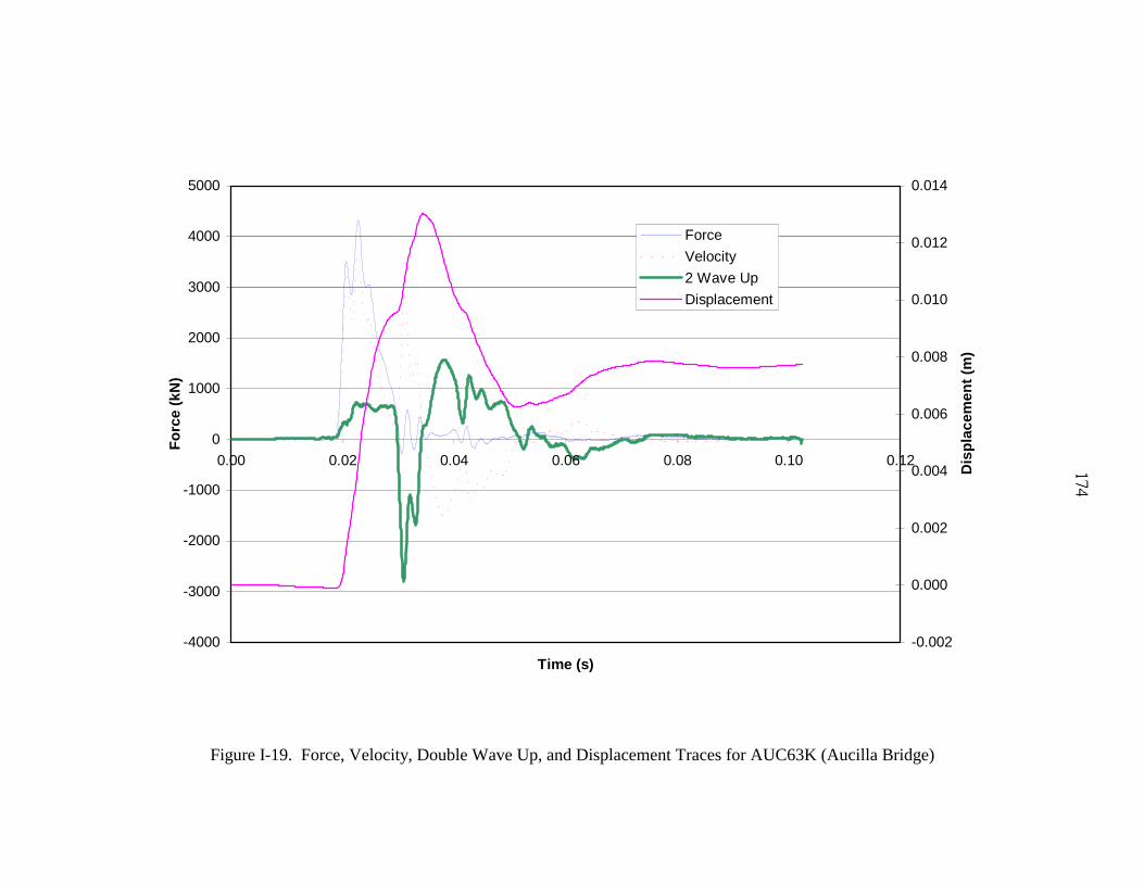
-4000
-3000
-2000
-1000
0
1000
2000
3000
4000
5000
0.00 0.02 0.04 0.06 0.08 0.10 0.12
Time (s)
For
ce (
kN)
-0.002
0.000
0.002
0.004
0.006
0.008
0.010
0.012
0.014
Dis
plac
emen
t (m
)
Force
Velocity
2 Wave Up
Displacement
Figure I-19. Force, Velocity, Double Wave Up, and Displacement Traces for AUC63K (Aucilla Bridge)
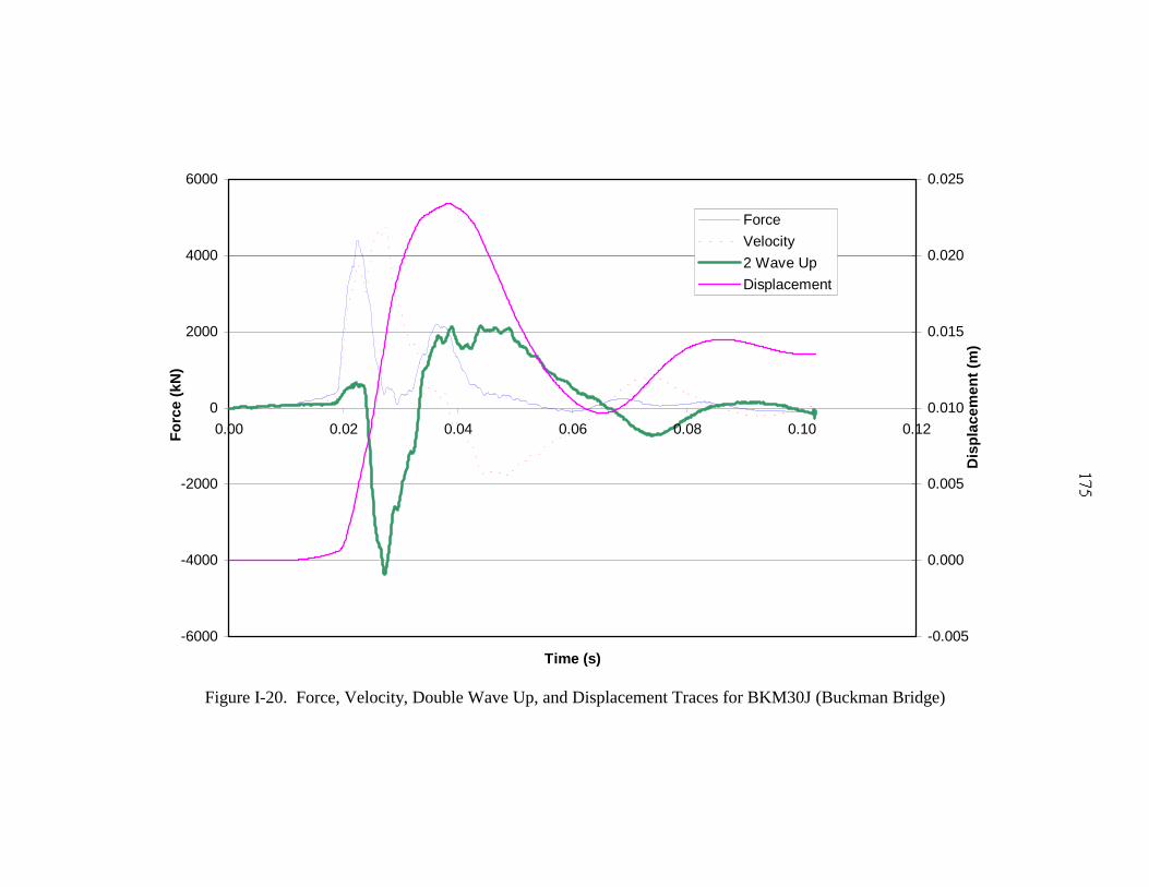
-6000
-4000
-2000
0
2000
4000
6000
0.00 0.02 0.04 0.06 0.08 0.10 0.12
Time (s)
For
ce (
kN)
-0.005
0.000
0.005
0.010
0.015
0.020
0.025
Dis
plac
emen
t (m
)
Force
Velocity
2 Wave Up
Displacement
Figure I-20. Force, Velocity, Double Wave Up, and Displacement Traces for BKM30J (Buckman Bridge)
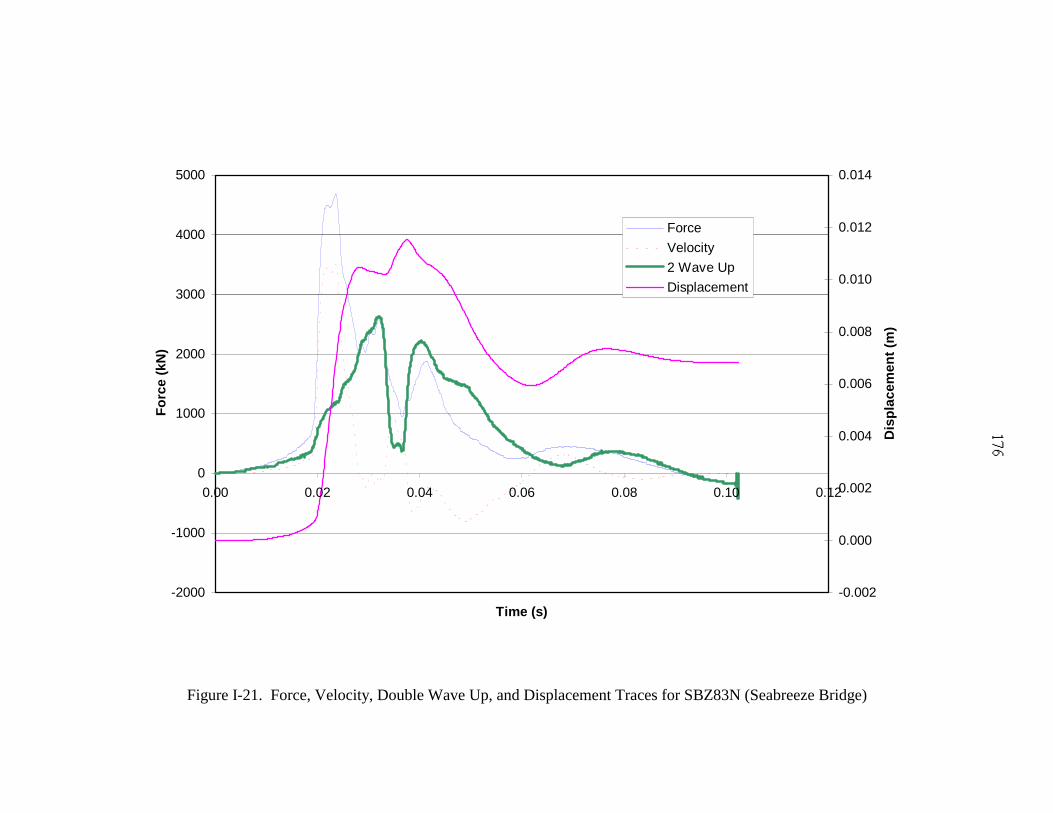
-2000
-1000
0
1000
2000
3000
4000
5000
0.00 0.02 0.04 0.06 0.08 0.10 0.12
Time (s)
For
ce (
kN)
-0.002
0.000
0.002
0.004
0.006
0.008
0.010
0.012
0.014
Dis
plac
emen
t (m
)
Force
Velocity
2 Wave Up
Displacement
Figure I-21. Force, Velocity, Double Wave Up, and Displacement Traces for SBZ83N (Seabreeze Bridge)
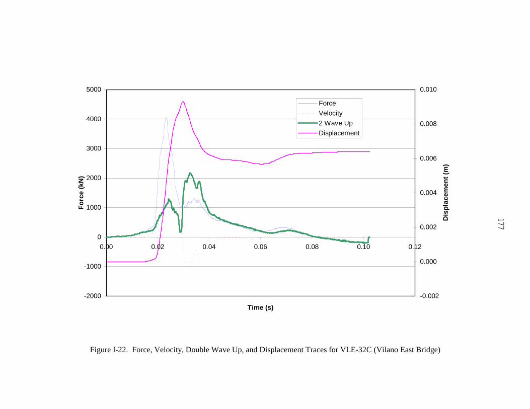
-2000
-1000
0
1000
2000
3000
4000
5000
0.00 0.02 0.04 0.06 0.08 0.10 0.12
Time (s)
For
ce (
kN)
-0.002
0.000
0.002
0.004
0.006
0.008
0.010
Dis
plac
emen
t (m
)
Force
Velocity
2 Wave Up
Displacement
Figure I-22. Force, Velocity, Double Wave Up, and Displacement Traces for VLE-32C (Vilano East Bridge)
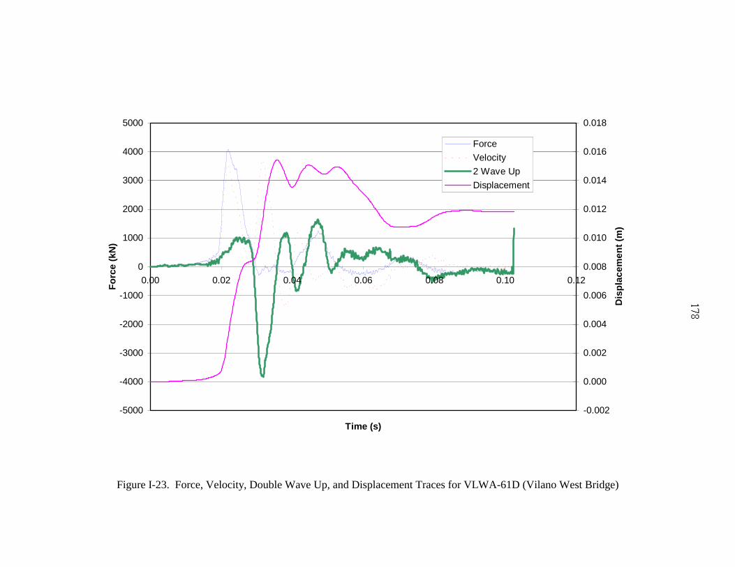
-5000
-4000
-3000
-2000
-1000
0
1000
2000
3000
4000
5000
0.00 0.02 0.04 0.06 0.08 0.10 0.12
Time (s)
For
ce (
kN)
-0.002
0.000
0.002
0.004
0.006
0.008
0.010
0.012
0.014
0.016
0.018
Dis
plac
emen
t (m
)
Force
Velocity
2 Wave Up
Displacement
Figure I-23. Force, Velocity, Double Wave Up, and Displacement Traces for VLWA-61D (Vilano West Bridge)

APPENDIX J
OUTPUT FILE FOR SUGGESTED METHOD & GRL PROCEDURE (FORTRAN)
180
*************************************************************˝********** UNIVERSITY OF FLORIDA **********˝********** FLORIDA DEPARTMENT OF TRANSPORTATION ******************** ********************SUGGESTED METHOD FOR DETERMINE SKIN & TIP******************** CAPACITIES / METHOD 1 ***********************************************************************
<<<<< PILE INFORMATION >>>>>
LENGTH = 29.76 mWAVESPEED = 4643.00 m/sMODU = 51750160.00 kN/m2AREA = .42 m2DT TIME = .00010 s
TIME VEL FOR ZVEL DISP 2 WAVE UP (s) (m/s) (kN) (kN) (m) (kN)
.0001 .000 .000 .000 .00000 .000 .0002 .000 .000 .000 .00000 .000 .0003 .000 .000 .000 .00000 .000 .0004 .000 .000 .000 .00000 .000 .0005 .000 .000 .000 .00000 .000 .0006 .000 .000 .000 .00000 .000 .0007 .000 .000 .000 .00000 .000 .0008 .000 .000 .000 .00000 .000 .0009 .000 .000 .000 .00000 .000 .0010 .000 .000 .000 .00000 .000 .0011 .000 .000 .000 .00000 .000 .0012 .000 .000 .000 .00000 .000 .0013 .000 .000 .000 .00000 .000 .0014 .000 .000 .000 .00000 .000 .0015 .000 .000 .000 .00000 .000 .0016 .000 .000 .000 .00000 .000 .0017 .000 .000 .000 .00000 .000 .0018 .000 .000 .000 .00000 .000 .0019 .000 .000 .000 .00000 .000 .0020 .000 .000 .000 .00000 .000 .0021 .000 .000 .000 .00000 .000 .0022 .000 .000 .000 .00000 .000 .0023 .000 .000 .000 .00000 .000 .0024 .000 .000 .000 .00000 .000 .0025 .000 .000 .000 .00000 .000 .0026 .000 .000 .000 .00000 .000 .0027 .000 .000 .000 .00000 .000 .0028 .000 .000 .000 .00000 .000 .0029 .000 .000 .000 .00000 .000 .0030 .000 .000 .000 .00000 .000 .0031 .000 .000 .000 .00000 .000 .0032 .000 .000 .000 .00000 .000 .0033 .000 .000 .000 .00000 .000 .0034 .000 .000 .000 .00000 .000 .0035 .000 .000 .000 .00000 .000 .0036 .000 .000 .000 .00000 .000 .0037 .000 .000 .000 .00000 .000 .0038 .000 .000 .000 .00000 .000 .0039 .000 .000 .000 .00000 .000
181
.0040 .000 .000 .000 .00000 .000 .0041 .000 .000 .000 .00000 .000 .0042 .000 .000 .000 .00000 .000 .0043 .000 .000 .000 .00000 .000 .0044 .000 .000 .000 .00000 .000 .0045 .000 .000 .000 .00000 .000 .0046 .000 .000 .000 .00000 .000 .0047 .000 .000 .000 .00000 .000 .0048 .000 .000 .000 .00000 .000 .0049 .000 .000 .000 .00000 .000 .0050 .000 .000 .000 .00000 .000 .0051 .000 .000 .000 .00000 .000 .0052 .000 .000 .000 .00000 .000 .0053 .000 .000 .000 .00000 .000 .0054 .000 .000 .000 .00000 .000 .0055 .000 .000 .000 .00000 .000 .0056 .000 .000 .000 .00000 .000 .0057 .000 .000 .000 .00000 .000 .0058 .000 .000 .000 .00000 .000 .0059 .000 .000 .000 .00000 .000 .0060 .000 .000 .000 .00000 .000 .0061 .000 .000 .000 .00000 .000 .0062 .000 .000 .000 .00000 .000 .0063 .000 .000 .000 .00000 .000 .0064 .000 .000 .000 .00000 .000 .0065 .000 .000 .000 .00000 .000 .0066 .000 .000 .000 .00000 .000 .0067 .000 .000 .000 .00000 .000 .0068 .000 .000 .000 .00000 .000 .0069 .000 .000 .000 .00000 .000 .0070 .000 .000 .000 .00000 .000 .0071 .000 .000 .000 .00000 .000 .0072 .000 .000 .000 .00000 .000 .0073 .000 .000 .000 .00000 .000 .0074 .000 .000 .000 .00000 .000 .0075 .000 .000 .000 .00000 .000 .0076 .000 .000 .000 .00000 .000 .0077 .000 .000 .000 .00000 .000 .0078 .000 .000 .000 .00000 .000 .0079 .000 .000 .000 .00000 .000 .0080 .000 .000 .000 .00000 .000 .0081 .000 .000 .000 .00000 .000 .0082 .000 .000 .000 .00000 .000 .0083 .000 .000 .000 .00000 .000 .0084 .000 .000 .000 .00000 .000 .0085 .000 46.440 .000 .00000 46.440 .0086 .000 46.440 .000 .00000 46.440 .0087 .000 46.440 .000 .00000 46.440 .0088 .000 46.440 .000 .00000 46.440 .0089 .000 46.440 .000 .00000 46.440 .0090 .000 46.440 .000 .00000 46.440 .0091 .000 46.440 .000 .00000 46.440 .0092 .000 46.440 .000 .00000 46.440 .0093 .000 46.440 .000 .00000 46.440 .0094 .000 46.440 .000 .00000 46.440 .0095 .000 46.440 .000 .00000 46.440 .0096 .000 46.440 .000 .00000 46.440 .0097 .000 46.440 .000 .00000 46.440 .0098 .000 46.440 .000 .00000 46.440 .0099 .000 46.440 .000 .00000 46.440 .0100 .000 46.440 .000 .00000 46.440
182
.0101 .000 46.440 .000 .00000 46.440 .0102 .000 46.440 .000 .00000 46.440 .0103 .000 46.440 .000 .00000 46.440 .0104 .000 46.440 .000 .00000 46.440 .0105 .000 92.881 .000 .00000 92.881 .0106 .000 92.881 .000 .00000 92.881 .0107 .000 92.881 .000 .00000 92.881 .0108 .000 92.881 .000 .00000 92.881 .0109 .000 92.881 .000 .00000 92.881 .0110 .000 92.881 .000 .00000 92.881 .0111 .000 92.881 .000 .00000 92.881 .0112 .000 92.881 .000 .00000 92.881 .0113 .000 92.881 .000 .00000 92.881 .0114 .000 92.881 .000 .00000 92.881 .0115 .010 92.881 46.440 .00000 46.440 .0116 .010 92.881 46.440 .00000 46.440 .0117 .010 92.881 46.440 .00000 46.440 .0118 .010 92.881 46.440 .00000 46.440 .0119 .010 92.881 46.440 .00000 46.440 .0120 .010 92.881 46.440 .00001 46.440 .0121 .010 92.881 46.440 .00001 46.440 .0122 .010 92.881 46.440 .00001 46.440 .0123 .010 92.881 46.440 .00001 46.440 .0124 .010 92.881 46.440 .00001 46.440 .0125 .010 139.321 46.440 .00001 92.881 .0126 .010 139.321 46.440 .00001 92.881 .0127 .010 139.321 46.440 .00001 92.881 .0128 .010 139.321 46.440 .00001 92.881 .0129 .010 139.321 46.440 .00001 92.881 .0130 .010 139.321 46.440 .00002 92.881 .0131 .010 139.321 46.440 .00002 92.881 .0132 .010 139.321 46.440 .00002 92.881 .0133 .010 139.321 46.440 .00002 92.881 .0134 .010 139.321 46.440 .00002 92.881 .0135 .010 139.321 46.440 .00002 92.881 .0136 .010 139.321 46.440 .00002 92.881 .0137 .010 139.321 46.440 .00002 92.881 .0138 .010 139.321 46.440 .00002 92.881 .0139 .010 139.321 46.440 .00002 92.881 .0140 .010 139.321 46.440 .00003 92.881 .0141 .010 139.321 46.440 .00003 92.881 .0142 .010 139.321 46.440 .00003 92.881 .0143 .010 139.321 46.440 .00003 92.881 .0144 .010 139.321 46.440 .00003 92.881 .0145 .020 185.761 92.881 .00003 92.881 .0146 .020 185.761 92.881 .00003 92.881 .0147 .020 185.761 92.881 .00003 92.881 .0148 .020 185.761 92.881 .00004 92.881 .0149 .020 185.761 92.881 .00004 92.881 .0150 .020 185.761 92.881 .00004 92.881 .0151 .020 185.761 92.881 .00004 92.881 .0152 .020 185.761 92.881 .00004 92.881 .0153 .020 185.761 92.881 .00005 92.881 .0154 .020 185.761 92.881 .00005 92.881 .0155 .020 232.201 92.881 .00005 139.321 .0156 .020 232.201 92.881 .00005 139.321 .0157 .020 232.201 92.881 .00005 139.321 .0158 .020 232.201 92.881 .00006 139.321 .0159 .020 232.201 92.881 .00006 139.321 .0160 .020 232.201 92.881 .00006 139.321 .0161 .040 232.201 185.761 .00006 46.440
183
.0162 .030 232.201 139.321 .00007 92.881 .0163 .030 232.201 139.321 .00007 92.881 .0164 .030 232.201 139.321 .00007 92.881 .0165 .030 278.642 139.321 .00008 139.321 .0166 .030 278.642 139.321 .00008 139.321 .0167 .030 278.642 139.321 .00008 139.321 .0168 .030 278.642 139.321 .00009 139.321 .0169 .030 278.642 139.321 .00009 139.321 .0170 .030 278.642 139.321 .00009 139.321 .0171 .030 325.082 139.321 .00009 185.761 .0172 .030 325.082 139.321 .00010 185.761 .0173 .030 325.082 139.321 .00010 185.761 .0174 .040 325.082 185.761 .00010 139.321 .0175 .040 325.082 185.761 .00011 139.321 .0176 .040 325.082 185.761 .00011 139.321 .0177 .040 371.522 185.761 .00012 185.761 .0178 .040 371.522 185.761 .00012 185.761 .0179 .040 371.522 185.761 .00012 185.761 .0180 .040 371.522 185.761 .00013 185.761 .0181 .050 417.963 232.201 .00013 185.761 .0182 .040 417.963 185.761 .00014 232.201 .0183 .050 417.963 232.201 .00014 185.761 .0184 .050 464.403 232.201 .00015 232.201 .0185 .060 510.843 278.642 .00015 232.201 .0186 .070 557.283 325.082 .00016 232.201 .0187 .080 650.164 371.522 .00017 278.642 .0188 .100 743.044 464.403 .00017 278.642 .0189 .140 928.806 650.164 .00019 278.642 .0190 .150 1114.567 696.604 .00020 417.963 .0191 .200 1300.328 928.806 .00022 371.522 .0192 .230 1439.649 1068.126 .00024 371.522 .0193 .280 1671.850 1300.328 .00027 371.522 .0194 .310 1950.492 1439.649 .00030 510.843 .0195 .360 2182.693 1671.850 .00033 510.843 .0196 .420 2461.335 1950.492 .00037 510.843 .0197 .480 2832.857 2229.133 .00041 603.724 .0198 .530 3111.499 2461.335 .00046 650.164 .0199 .600 3436.581 2786.417 .00052 650.164 .0200 .640 3808.103 2972.178 .00058 835.925 .0201 .740 4179.625 3436.581 .00065 743.044 .0202 .800 4551.147 3715.222 .00073 835.925 .0203 .880 4829.789 4086.745 .00081 743.044 .0204 .920 5108.431 4272.506 .00090 835.925 .0205 .980 5340.632 4551.147 .00100 789.485 .0206 1.020 5526.393 4736.909 .00110 789.485 .0207 1.060 5712.154 4922.670 .00120 789.485 .1006 -.010 -278.642 -46.440 -.00013 -232.201 .1007 -.010 -278.642 -46.440 -.00013 -232.201 .1008 -.010 -278.642 -46.440 -.00013 -232.201 .1009 -.010 -278.642 -46.440 -.00013 -232.201 .1010 -.010 -325.082 -46.440 -.00013 -278.642 .1011 -.010 -278.642 -46.440 -.00013 -232.201 .1012 -.010 -325.082 -46.440 -.00013 -278.642 .1013 -.010 -278.642 -46.440 -.00013 -232.201 .1014 -.010 -325.082 -46.440 -.00013 -278.642 .1015 -.010 -278.642 -46.440 -.00013 -232.201 .1016 -.010 -325.082 -46.440 -.00014 -278.642 .1017 .000 -278.642 .000 -.00014 -278.642 .1018 .000 -325.082 .000 -.00014 -325.082 .1019 .000 -278.642 .000 -.00014 -278.642 .1020 -.010 -325.082 -46.440 -.00014 -278.642
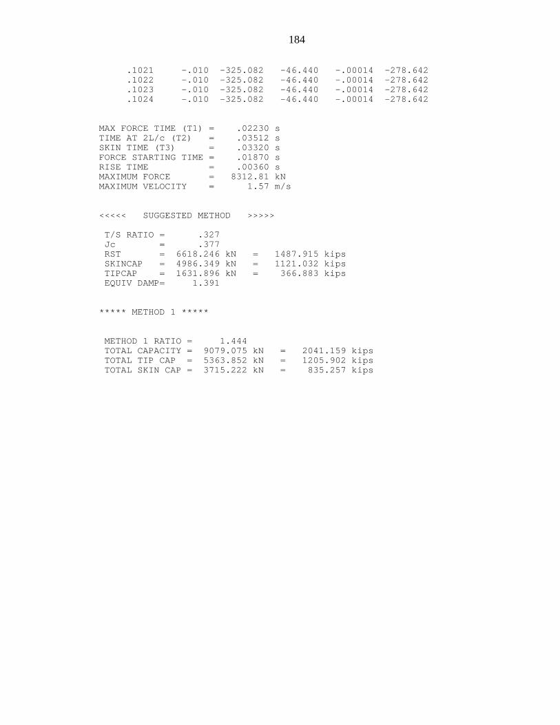
184
.1021 -.010 -325.082 -46.440 -.00014 -278.642 .1022 -.010 -325.082 -46.440 -.00014 -278.642 .1023 -.010 -325.082 -46.440 -.00014 -278.642 .1024 -.010 -325.082 -46.440 -.00014 -278.642
MAX FORCE TIME (T1) = .02230 sTIME AT 2L/c (T2) = .03512 sSKIN TIME (T3) = .03320 sFORCE STARTING TIME = .01870 sRISE TIME = .00360 sMAXIMUM FORCE = 8312.81 kNMAXIMUM VELOCITY = 1.57 m/s
<<<<< SUGGESTED METHOD >>>>>
T/S RATIO = .327 Jc = .377 RST = 6618.246 kN = 1487.915 kips SKINCAP = 4986.349 kN = 1121.032 kips TIPCAP = 1631.896 kN = 366.883 kips EQUIV DAMP= 1.391
***** METHOD 1 *****
METHOD 1 RATIO = 1.444 TOTAL CAPACITY = 9079.075 kN = 2041.159 kips TOTAL TIP CAP = 5363.852 kN = 1205.902 kips TOTAL SKIN CAP = 3715.222 kN = 835.257 kips
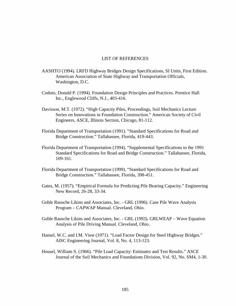
185
LIST OF REFERENCES
AASHTO (1994). LRFD Highway Bridges Design Specifications, SI Units, First Edition.American Association of State Highway and Transportation Officials,Washington, D.C.
Coduto, Donald P. (1994). Foundation Design Principles and Practices. Prentice HallInc., Englewood Cliffs, N.J., 403-416.
Davisson, M.T. (1972). “High Capacity Piles, Proceedings, Soil Mechanics LectureSeries on Innovations in Foundation Construction.” American Society of CivilEngineers, ASCE, Illinois Section, Chicago, 81-112.
Florida Department of Transportation (1991). “Standard Specifications for Road andBridge Construction.” Tallahassee, Florida, 419-443.
Florida Department of Transportation (1994). “Supplemental Specifications to the 1991Standard Specifications for Road and Bridge Construction.” Tallahassee, Florida,109-161.
Florida Department of Transportation (1999). “Standard Specifications for Road andBridge Construction.” Tallahassee, Florida, 398-451.
Gates, M. (1957). “Empirical Formula for Predicting Pile Bearing Capacity.” EngineeringNew Record, 26-28, 33-34.
Goble Rausche Likins and Associates, Inc. - GRL (1996). Case Pile Wave AnalysisProgram – CAPWAP Manual. Cleveland, Ohio.
Goble Rausche Likins and Associates, Inc. - GRL (1993). GRLWEAP – Wave EquationAnalysis of Pile Driving Manual. Cleveland, Ohio.
Hansel, W.C. and I.M. Viest (1971). “Load Factor Design for Steel Highway Bridges.”AISC Engineering Journal, Vol. 8, No. 4, 113-123.
Housel, William S. (1966). “Pile Load Capacity: Estimates and Test Results.” ASCEJournal of the Soil Mechanics and Foundations Division, Vol. 92, No. SM4, 1-30.

186
Likins, Garland E. and Hussein, Mohamad (1988). “A Summary of the Pile DrivingAnalyzer Capacity Methods – Past and Present.” The Eleventh Pile DrivingAnalyzer User’s Seminar, Cleveland, Ohio.
Paikowsky, S.G., Regan, J.E., and McDonnell, J.J. (1994). “A simplified field Method forCapacity Evaluation of Driven Piles.” Publication No. FHWA-RD-94-042,Federal Highway Administration, Washington, D.C.
Pile Dynamics, Inc. (1992). Pile Driving Analyzer (PDA) Manual. Cleveland, Ohio.
Rosenblueth, E. and Esteva, L. (1972). “Reliability Basis for Some Mexican Codes.” ACIPublication SP-31, American Concrete Institute, Detroit, Mi.
Sakai, T., Sawai, H., and Shioi, Y. (1996). “Theoretical Analysis of the Pile DrivingFormula.” Proceeding, 5th International Conference on the Application of StressWave Theory to Piles. September 11-13, 1996. Orlando, Florida, 81-88.
Willington, A.M. (1893). Piles and Pile-Driving. Engineering News Publishing Co., NewYork.
Withiam, J.L., Voytko, E.P., Barker, R.M., Duncan, J.M., Kelly, B.C., Musser, S.C., andElias, V. (1997). Load and Resistance Factor Design (LRFD) for Highway BridgeStructures. FHWA Report DTFH61-94-C-00098. Federal HighwayAdministration, Washington, D.C.

187
BIOGRAPHICAL SKETCH
Ariel Perez was born February 21, 1971, in La Havana, Cuba, to Antonio Perez
Rodriguez and Mirtha Felipa Perez Castro. He attended elementary school in Marianao
until end of sixth grade when he moved with his family to Tenerife, Spain. After one and
a half year living at the Canary Islands, he returned to America, San Juan, Puerto Rico,
where he graduated from Colegio Bautista de Carolina High School with honors.
On August 1990, Mr. Perez entered a pre-engineering program at the University
of Puerto Rico, Bayamón Campus (CUTB) where he obtained an Associate in Science
and Mathematics degree. Subsequently, he transferred to the University of Puerto Rico,
Mayagüez Campus (RUM). While attending RUM, he enrolled in the Cooperative
Education Program (COOP). As a COOP student he worked for almost one year with the
U.S. Environmental Protection Agency (EPA) – Region II, Edison, New Jersey. On May
1996, he earned his Bachelor of Science Degree in Civil Engineering with honors (Magna
Cum Laude) and received the Ettienne Totti award, which is the Civil Engineering
Department award to the best undergraduate student.
After graduation, he worked for CMA Architects & Engineers, a prestigious
engineering consulting firm established in San Juan, Puerto Rico since 1959, who
awarded him with the CMA Architects & Engineers grant for graduate studies. Desirous
of acquiring a higher level of knowledge as engineer, he decided to pursue a Master of
Engineering degree in the area of Geotechnical Engineering at the University of Florida.

188
Ariel Perez is a Registered Professional Engineer in Puerto Rico, and a Tau Beta
Pi member (Puerto Rico Alpha Chapter).


![Highway Bridge Loads and Load Distributionfreeit.free.fr/Bridge Engineering HandBook/ch06.pdf · Load and Resistance Factor Design (LRFD) Specifications [1]. Stream flow, ice loads,](https://img.pdfslide.net/doc/110x75/5a7013757f8b9a9d538b9e27/highway-bridge-loads-and-load-distributionfreeitfreefrbridge-engineering-handbookch06pdfpdf.jpg)