Local and Global Parameter Identi–cation in DSGE … · Local and Global Parameter Identi–cation in DSGE Models Allowing for Indeterminacy ... December 19, 2012; this version:

Local and Global Parameter Identi�cation in DSGE ModelsAllowing for Indeterminacy�

Zhongjun Quy

Boston University

Denis Tkachenkoz

National University of Singapore

December 19, 2012; this version: July 31, 2014

Abstract

This paper presents a uni�ed framework for analyzing local and global identi�cation in loglinearized DSGE models that encompasses both determinacy and indeterminacy. The analysisis conducted from a frequency domain perspective. First, for local identi�cation, it presentsnecessary and su¢ cient conditions for: (1) the identi�cation of the structural parameters alongwith the sunspot parameters, (2) the identi�cation of the former irrespective of the latter and(3) the identi�cation of the former conditional on the latter. These conditions apply to bothsingular and nonsingular models and also permit checking whether a subset of frequencies candeliver identi�cation. Second, for global identi�cation, the paper considers a frequency domainexpression for the Kullback-Leibler distance between two DSGE models and shows that globalidenti�cation fails if and only if the minimized distance equals zero. As a by-product, it deliversparameter values that yield observational equivalence under identi�cation failure. This conditionrequires nonsingularity but can be applied to nonsingular subsystems and across models withdi¤erent structures. Third, to develop a further understanding of the strength of identi�cation,the paper proposes a measure for the empirical closeness between two DSGE models. Themeasure gauges the feasibility of distinguishing one model from another using likelihood ratiotests based on a �nite number of observations generated by the two models. The theory isillustrated using two small scale and one medium scale DSGE models. The results document thatparameters can be identi�ed under indeterminacy but not determinacy, that di¤erent monetarypolicy rules can be (nearly) observationally equivalent, and that identi�cation properties candi¤er substantially between small and medium scale models.Keywords: Dynamic stochastic general equilibrium models, frequency domain, global identi�-cation, multiple equilibria, spectral density.JEL Classi�cation: C10, C30, C52, E1,E3.

�We are grateful to Bertille Antoine, Jesús Fernández-Villaverde, Frank Kleibergen, Arthur Lewbel, Eric Renault,Yixiao Sun and seminar participants at Academia Sinica, BC, Brown, MSU, Birmingham Macroeconomics andEconometrics Conference, CIREQ Econometrics Conference, Econometric Society Winter Meeting and NBER summerinstitute for useful comments and suggestions.

yDepartment of Economics, Boston University, 270 Bay State Rd., Boston, MA, 02215 ([email protected]).zDepartment of Economics, National University of Singapore ([email protected]).

1 Introduction

Dynamic Stochastic General Equilibrium (DSGE) models provide a uni�ed framework for analyzing

business cycles, understanding monetary policy and forecasting. An inherent feature of such models

is that, under some parameter values, there can exist a continuum of stable solutions, all satisfying

the same set of conditions for equilibrium. This feature, called indeterminacy, can be valuable

for understanding the sources and dynamics of macroeconomic �uctuations. For example, Lubik

and Schorfheide (2004) considered a prototypical DSGE model and argued that indeterminacy

is consistent with the way US monetary policy was conducted over the period 1960:I to 1979:II.

Related work in this area includes Leeper (1991), Clarida, Galí and Gertler (2000), Benhabib,

Schmitt-Grohé and Uribe (2001), Boivin and Giannoni (2006), Benati and Surico (2009), Mavroeidis

(2010) and Cochrane (2011, 2014). Benhabib and Farmer (1999) documented various economic

mechanisms leading to indeterminacy, suggesting a further integration of this feature into the

DSGE theory.

Parameter identi�cation in DSGE models is important for both calibration and formal statisti-

cal analysis. Substantial progress has been made recently. Canova and Sala (2009) documented the

types of identi�cation issues that can arise when analyzing DSGE models. Iskrev (2010) gave su¢ -

cient conditions, while Komunjer and Ng (2011) and Qu and Tkachenko (2012) provided necessary

and su¢ cient conditions for local identi�cation. However, these conditions have two substantial

limitations. First, they assume determinacy. Second, they are silent about global identi�cation.

Furthermore, the DSGE literature contains no published work that provides necessary and su¢ cient

conditions for global identi�cation, even under determinacy, except when the solution can be pre-

sented as a �nite order vector autoregression (Rubio-Ramírez, Waggoner and Zha, 2010 and Fukaµc,

Waggoner and Zha, 2007). This paper aims to make progress in three directions. First, it presents

necessary and su¢ cient conditions for local identi�cation that encompass both determinacy and

indeterminacy. Second, it provides a necessary and su¢ cient condition for global identi�cation.

Third, it proposes a measure to gauge the empirical closeness of DSGE models, re�ecting the

feasibility of distinguishing one model from another based on �nite sample sizes.

The local identi�cation analysis builds on the work of Lubik and Schorfheide (2003) and extends

the results in Qu and Tkachenko (2012). It proceeds in three steps. First, it de�nes an augmented

parameter vector that consists of both the structural (i.e., those appearing in the log linearized

structural model) and the sunspot (i.e., those appearing only under indeterminacy) parameters.

Next, it constructs a spectral density which characterizes the second order properties of the full set

1

of solutions. Third, it treats this spectral density as an in�nite dimensional mapping, as in Qu and

Tkachenko (2012), studying its properties under local perturbation of parameter values to obtain

characterizing conditions for identi�cation. The analysis exploits two features of DSGE models.

That is, the models are general equilibrium models and the solutions are vector linear processes. The

�rst feature makes the issue of observed exogenous processes irrelevant. Together, the two features

imply that the spectral density summarizes all relevant information under normality, which holds

under both determinacy and indeterminacy.

The results on local identi�cation cover three situations. (1) The identi�cation of both the

structural and the sunspot parameters. This reveals the possibility of locally determining both the

parameters describing technology and preferences and those governing the equilibrium beliefs of

agents. (2) The identi�cation of the structural parameters without making statements about the

identi�cation of the sunspot parameters. This shows whether it is possible to locally determine

the parameters describing technology and preferences, even though the equilibrium beliefs may

be unidenti�able. (3) The identi�cation of the structural parameters conditional on the value of

the sunspot parameters. This reveals whether it is possible to locally determine the parameters

describing technology and preferences once we select a mechanism for equilibrium belief formation.

In each of the three situations, the paper provides necessary and su¢ cient conditions for identi-

�cation. In practice, the conditions can be applied sequentially. If the �rst condition is violated,

then the other two can be used to better understand the sources of identi�cation failure. All the

results allow arbitrary relationships between the number of observables and shocks, therefore are

applicable to both singular and nonsingular DSGE models. They permit latent state variables and

measurement errors and are relatively straightforward to compute.

The global identi�cation analysis in DSGE models faces two challenges. (1) The model�s solu-

tions are often not representable as regressions with a �nite number of predetermined regressors,

especially under indeterminacy. (2) The parameters interact in a highly nonlinear fashion. These

two features make the results in Rothenberg (1971, Sections 4-6) inapplicable. Exploring a di¤erent

route, this paper obtains the identi�cation condition by making further uses of the general equilib-

rium feature and vector linear structure of the solutions. First, it introduces a frequency domain

expression for the Kullback�Leibler distance between two DSGE models. This criterion depends

only on the spectral densities and the dimension of the observables, thus can be computed without

simulation or any reference to any data. Second, it shows that global identi�cation fails if and only

if the criterion equals zero when minimized over the relevant region of the parameter space. When

2

identi�cation fails, the condition delivers a set of parameter values that lead to observational equiv-

alence. Meanwhile, when global identi�cation holds, the minimized value is still informative about

the strength of the identi�cation. The latter feature is further exploited in the paper to develop

a measure for the empirical closeness between models. In relation to the literature, Fernández-

Villaverde and Rubio-Ramírez (2004) are among the �rst to consider the Kullback�Leibler distance

in the context of DSGE models. They showed that the parameter estimates obtained from Bayesian

methods converge to their pseudo true values and the best model under the Kullback�Leibler dis-

tance will receive the highest posterior probability. The current paper is the �rst that makes use

of the Kullback�Leibler distance for checking global identi�cation. The feasibility lies in the fea-

ture that its frequency domain expression only depends on the spectral densities, which are easily

computable even under indeterminacy, as illustrated later in the paper.

The proposed local and global identi�cation conditions can be compared along three dimensions.

First and broadly, identi�cation analysis can involve two types of questions with increasing levels

of complexity, i.e., parameter identi�cation conditional on the model structure and identi�cation

permitting di¤erent structures. In the current context, the former asks whether there exists a

di¤erent parameter value within the same DSGE structure that can lead to the same dynamics for

the observables. The latter asks whether an alternatively speci�ed DSGE structure (for example,

a model with a di¤erent monetary policy rule or with di¤erent shock processes) can generate the

same dynamic properties as some benchmark structure. The local identi�cation condition, here

and elsewhere in the literature, can only be used to address the �rst type of identi�cation question.

In contrast, the global condition proposed here can also address the second type. This is the only

condition in the DSGE literature with such a property. Second, the computational cost associated

with the global identi�cation condition can be substantially higher than in the case of the local

condition when the dimension of the parameter vector is high. Nevertheless, this paper provides

ample evidence showing that it can be e¤ectively implemented for both small scale and medium

scale DSGE models. Third, the global identi�cation condition requires the model to be nonsingular.

For singular systems, it can still be applied to nonsingular subsystems, as shown in the paper.

When global identi�cation holds, there may still exist parameter values that are di¢ cult to

distinguish based on �nite samples. For example, Del Negro and Schorfheide (2008) considered a

New Keynesian DSGE model and observed that the data provides similar support for a model with

moderate price and trivial wage rigidity and one in which both rigidities are high. In Section 7.2,

this paper �nds that apparently very di¤erent Taylor rule parameters can lead to near observational

3

equivalence in a model considered by Lubik and Schorfheide (2004). More generally, even models

with di¤erent structures (i.e., with di¤erent policy rules or di¤erent shock processes) can be similar

quantitatively. To address this issue, this paper develops a measure for the empirical closeness

between DSGE models. The measure gauges the feasibility of distinguishing one model from another

using likelihood ratio tests based on a �nite number of observations generated by the two models.

It has three features. First, it is straightforward to compute for general DSGE models. The

main computation cost is in solving the two models once and computing their respective spectral

densities. Second, its value always falls between 0 and 1 with a higher value indicating a greater

di¤erence. Third, it monotonically approaches one as the sample size increases if the Kullback�

Leibler criterion is positive. The development here is related to Hansen (2007) who, working from

a Bayesian decision making perspective, proposed to use Cherno¤�s (1952) information measure to

quantify statistical challenges for distinguishing between two models.

The above methods are applied to three DSGE models. The �rst two are small scale models

considered in An and Schorfheide (2007) and Lubik and Schorfheide (2004), while the third is the

medium scale model of Smets and Wouters (2007). Putting these three models together showcases

how identi�cation properties can di¤er within small scale models and between small and medium

scale models. The main �ndings can be summarized as follows. First, consider the model of

An and Schorfheide (2007). Previously, Qu and Tkachenko (2012) showed that the Taylor rule

parameters are locally unidenti�ed at a parameter value that yields determinacy. Here, the paper

considers a range of di¤erent values under indeterminacy and �nds consistently that the Taylor rule

parameters are globally identi�ed. Such a distinction in parameter identi�cation has previously

only been documented for models with analytical solutions. The result here shows that this can

occur in models of empirical relevance. When measuring the empirical distance between models

with di¤erent monetary policy rules, the method detects an expected in�ation rule that leads to

exact observational equivalence with the current in�ation rule. Meanwhile, there exists an output

growth rule that leads to near observational equivalence as the output gap rule. Both �ndings

hold under both determinacy and indeterminacy. Next, consider the model analyzed in Lubik and

Schorfheide (2004). In contrast to the previous model, the paper �nds that the parameters are

globally identi�ed at the posterior mean under both determinacy and indeterminacy. Meanwhile,

the exact and near observational equivalence between alternative monetary policy rules still persists.

Third, consider the model of Smets and Wouters (2007). The model is globally identi�ed at the

posterior mean under determinacy after �xing �ve parameters as in the original paper. However,

4

some parameters (i.e., the steady state elasticity of the capital adjustment cost function and the

elasticity of labor supply) are identi�ed only weakly. In contrast to the small scale models, the

exact and near observational equivalence between monetary policy rules are no longer present.

When measuring the empirical distance between models with di¤erent degrees of real and nominal

frictions, the results suggest that all eight frictions are empirically relevant in generating the model�s

dynamic properties. The least important frictions are, among the nominal frictions, the price and

wage indexation and, among the real frictions, the elasticity of capital utilization adjustment cost.

Interestingly, the conclusions reached regarding both the nominal and real frictions are consistent

with those obtained from a Bayesian perspective in Smets and Wouters (2007).

This paper expands the early literature on identi�cation in rational expectations models. There,

notable contributions include Wallis (1980), Pesaran (1981) and Blanchard (1982). Wallis (1980,

p.63) provided a rank condition for the local identi�cation of the structural parameters in a model

that features observable exogenous processes and lagged expectations (i.e., the structural equations

at time t include only conditional expectations formed at t�1). These two features make the modele¤ectively static. Pesaran (1981, Theorem 1) considered the same model and provided a necessary

and su¢ cient condition for global identi�cation of the structural parameters in a particular struc-

tural equation. He also considered models under indeterminacy. However, no formal identi�cation

conditions were provided for this case. Blanchard (1982) extended Wallis�(1980) analysis to �rst-

order dynamic linear models. The above analyses share a common feature. That is, the solutions

are �nite order static regressions or vector autoregressions. This makes identi�cation conditions for

standard simultaneous equations system applicable. Therefore, although their results shed some

light on the problem, their methods are not applicable to general DSGE models. This paper also

contributes to the literature that studies dynamic equilibrium models from a frequency domain

perspective. Related studies include Altug (1989), Christiano, Eichenbaum and Marshall (1991),

Sims (1993), Hansen and Sargent (1993), Watson (1993), Diebold, Ohanian and Berkowitz (1998),

Christiano and Vigfusson (2003) and Del Negro, Diebold and Schorfheide (2008). The current paper

is the �rst to study global identi�cation in DSGE models from the frequency domain perspective.

The paper is structured as follows. Section 2 discusses the model�s solutions and the spectral

density under indeterminacy. Sections 3 and 4 present results on local and global identi�cation,

respectively. Section 5 proposes an empirical distance measure. Section 6 discusses the application

of the results to (factor augmented) VARMA models. Section 7 provides some illustrative appli-

cations while Section 8 concludes. The paper has three appendices. Appendix A contains details

5

on solving the model under indeterminacy following Lubik and Schorfheide (2003). Appendix B

outlines the model of Smets and Wouters (2007). All proofs are included in Appendix C.

The following notation is used. i is the imaginary unit. jjxjj is the Euclidean norm of a vector

x. jjXjj is the vector induced norm for a complex valued matrix X. X� stands for its conjugate

transpose while X 0 is the transpose without conjugation. If f� 2 Rk is a di¤erentiable function

of � 2 Rp, then @f�0=@�0 is a k-by-p matrix of partial derivatives evaluated at �0. �!d�signi�es

convergence in distribution and O(�) and o(�) are the usual symbols for orders of magnitude.

2 The spectrum of a DSGE model under indeterminacy

Suppose a DSGE model has been log linearized around its steady state (Sims, 2002):

�0St = �1St�1 +"t +��t; (1)

where St is a vector that includes the endogenous variables, the conditional expectations and

variables from exogenous shock processes if they are serially correlated. The vector "t contains

serially uncorrelated structural shocks and �t contains expectation errors. The elements of �0;�1;

and � are functions of the structural parameters in the model. Depending on the properties of

�0 and �1, the system can have none, a unique or multiple stable solutions. This paper assumes

at least one stable solution exists and focuses on such cases. For local identi�cation analysis, the

relationship between the number of endogenous variables and structural shocks is allowed to be

arbitrary, that is, the system can be singular.

Under indeterminacy, the structural parameters alone do not uniquely determine the dynamics

(i.e., the spectral density or the autocovariances) of the observables. This constitutes a conceptual

challenge for analyzing identi�cation. We take three key steps to overcome this obstacle. First,

the result in Lubik and Schorfheide (2003) is applied to obtain a representation for the full set of

solutions under indeterminacy. We also amend their procedure to allow the degree of indeterminacy

to exceed one. Second, the parameter space is augmented to include the sunspot parameters in

addition to the structural parameters. Third, utilizing the augmented parameter space, we compute

the unique spectral density which fully characterizes the second order properties of the observables.

This spectral density is easily computable and serves as the main instrument for the identi�cation

analysis in this paper. The details of the three steps are as follows.

6

Step 1. Model solution under indeterminacy. Lubik and Schorfheide (2003) showed that

under indeterminacy, the full set of solutions can be represented as

St = �1St�1 +�""t +��t; (2)

or equivalently,

St = (1��1L)�1[�" ��]

0@ "t

�t

1A ;

where L denotes the lag operator. Appendix A contains an alternative derivation of this represen-

tation using an elementary result in matrix algebra (see the discussion between (A.5) and (A.7)).

There, the reduced column echelon form is used to represent the indeterminacy space when the

dimension of the latter exceeds one. In the above, the matrices �1, �" and �� depend only on

�0;�1; and �, therefore are functions of the structural parameters only. The dimension of ��,

called the degree of indeterminacy, is also determined by the structural parameters. As in the

literature, the vector �t is labeled as sunspot shocks.

It is important to emphasize that the DSGE model alone imposes little restriction on �t. It

needs to be a martingale di¤erence, i.e., Et�t+1 = 0, however can be arbitrarily contemporaneously

correlated with the fundamental shocks "t. Intuitively, the properties of �t depend on how agents

form their expectations, which, under indeterminacy, is not fully revealed by the structural model

itself. In light of this, we write

�t =M"t +e�tand make the following assumption, allowing �t to be contemporaneously correlated with "t, being

conditional heteroskedastic (e.g., as in GARCH type models) with an arbitrary distribution.

Assumption 1 E�e�te�0t� = �� with 0 < jj��jj < 1, jjM jj < 1, E

�"te�0s� = 0 for all t,s and

E�e�te�0s� = 0 for all t 6= s.

Step 2. Parameter augmentation. Let �D be a p-by-1 vector consisting of all the structural

parameters in (1). Let �U be a q-by-1 vector consisting of the sunspot parameters:

�U =

0@ vec (��)

vec (M)

1A :

De�ne an augmented parameter vector:

� =

0@ �D

�U

1A :

7

Step 3. Computing the spectral density under indeterminacy. In practice, the estimation

or calibration is typically based on a subset of St or some linear transformations involving the current

and lagged values of St. To match such a practice, we let A(L) denote a matrix of �nite order lag

polynomials to specify the observables and write

Yt (�) = A(L)St = H(L; �)

0@ "t

�t

1A ; (3)

where

H(L; �) = A(L)(1��1L)�1[�" ��]: (4)

In the above notation, the observables are explicitly indexed by � to signify that their dynamic

properties will depend on both the structural and the sunspot parameters. The matrix A(L)

permits analyzing models with latent endogenous variables such as Smets and Wouters (2003,

2007). In these two models, St includes variables from a frictionless economy unobservable to the

econometrician. Such variables can be excluded simply by assigning zero entries in A(L).

Remark 1 The representation given by (3) and (4) demonstrates that Yt (�) is a vector linear

process driven by "t and �t and that it admits a vector moving average representation irrespective of

the number of shocks in the model. It often does not have a �nite order VAR representation. For

example, consider the leading case with a nonsingular system where the dimension of "t equals that

of Yt (�). Then, because of the presence of �t, the system is non-invertible, precluding any vector

autoregressive representations in the �rst place. The polynomial H(L; �) can be of in�nite order

due to the presence of A(L) and (1��1L)�1. This implies that the solutions can possess an in�nitenumber of reduced form parameters, making the latter unidenti�able without additional restrictions.

The spectral density of Yt(�) is, using (3) and (4),

f�(!) =1

2�H(exp(�i!); �)�(�)H(exp(�i!); �)�; (5)

where

�(�) =

0@ I 0

M I

1A0@ �" 0

0 ��

1A0@ I 0

M I

1A0 :Note that adding measurement errors would present no di¢ culty: suppose we observe Yt (�)+�t(�),

with �t(�) being measurement errors independent of Yt(�) with spectrum fm� (!), then the spectral

density of the observables is given by

f�(!) =1

2�H(exp(�i!); �)�(�)H(exp(�i!); �)� + fm� (!);

8

where H(�) is again de�ned by (4). The dimension of f�(!) is always nY -by-nY with nY being

the dimension of Yt (�). In particular, its dimension does not depend on the number of shocks or

whether there is indeterminacy.

Throughout the paper, we let fYtg denote a stochastic process whose spectral density is givenby f�0(!) for ! 2 [��; �]. The next assumption imposes some structure on the parameter spaceand the spectral density.

Assumption 2 (i) Assume �D 2 �D � Rp and � 2 � � Rp+q with �D and � being compact.

Assume �D0 is an interior point of �D and �0 is an interior point of � under indeterminacy. (ii)

The elements of the spectral density f�(!) are continuous in ! and continuous and di¤erentiable

in �; kf�(!)k � C <1 for all � 2 � and ! 2 [��; �]:

For local identi�cation, the compactness is not required. Also, (ii) only needs to hold in an

open neighborhood of �0 over ! 2 [��; �]. If unit roots are present in the DSGE model, then theassumption requires appropriately transforming the series prior to applying the methods.

Remark 2 In�uenced by Koopmans (1949, Abstract p. 125), the identi�cation analysis in econo-

metrics is often embedded in a hierarchical or two step formulation. First, the joint distribution of

the observations is written in terms of reduced form equations in which the parameters are always

identi�able. Second, the structural parameters are linked to the reduced form parameters through a

�nite number of time invariant restrictions, which uniquely matters for the identi�cation. However,

as discussed in Remark 1, in DSGE models the reduced form often does not possess a natural de-

�nition and the parameters involved can be unidenti�able. This motivates us to adopt Haavelmo�s

(1944, p. 99) formulation to write the joint distribution (more precisely, the spectral density) di-

rectly in terms of the structural parameters. This basic principle underlies the analysis of both local

and global identi�cation in this paper.

3 Local identi�cation

Komunjer and Ng (2011) and Qu and Tkachenko (2012) discussed potential challenges for studying

local identi�cation in DSGE models under determinacy. Similar challenges persist under indeter-

minacy. First, as stated in Remarks 1 and 2, Yt (�) in (3) in general does not admit a �nite order

vector autoregressive representation. This implies that the conventional approach of �rst locating

the identi�ed �nite dimensional reduced form parameters and then using them to back out the

structural ones breaks down. Second, because this is a general equilibrium model, it typically does

9

not include any observed exogenous processes. Therefore, the approach taken in the static context,

in particular that of Wallis (1980, p.63), also breaks down. Finally, depending on the number of

shocks in the model, the system can be singular. Singularity implies that the conventional in-

formation matrix is not well de�ned, therefore the rank condition in Rothenberg (1971) can be

inapplicable.

Our local identi�cation analysis builds on Qu and Tkachenko (2012). The key idea is that, under

indeterminacy, the solutions continue to be representable as a stationary vector linear process whose

second order properties continue to be fully characterized by the spectral density matrix f�(!) over

! 2 [��; �]. The elements of f�(!) can then be treated as mappings from the �nite dimensional

augmented parameter space to a space of complex valued functions de�ned over [��; �]. Localidenti�cation holds if and only if the overall mapping is locally injective. Once this perspective is

established, the results reported in this section then follow readily from those obtained in Section 3

in Qu and Tkachenko (2012). Nevertheless, we still present detailed discussions and proofs to ease

the understanding and to facilitate the methods�application in practice.

We start with the local identi�cation of both the structural and the sunspot parameters. In-

tuitively, if this holds, then it is potentially possible to locally determine both the parameters

describing technology and preferences (�D) and those governing the equilibrium beliefs of agents

(�U ).

De�nition 1 The parameter vector � is said to be locally identi�able from the second order prop-

erties of fYtg at � = �0 if there exists an open neighborhood of �0 in which f�1(!) = f�0(!) for all

! 2 [��; �] necessarily implies �1 = �0.

The above de�nition can also be stated equivalently in the time domain. Let f��(k)g1k=�1 be

the autocovariances of Yt (�) implied by the model. Then, � is said to be locally identi�able from

the second order properties of fYtg at � = �0 if there exists an open neighborhood of �0 in which

��1(k) = ��0(k) (k = 0;�1; :::) necessarily implies �1 = �0.

The mappings associated with the elements of f�(!) are in�nite dimensional and di¢ cult to

analyze directly. However, as observed in Qu and Tkachenko (2012), for local identi�cation it

su¢ ces to consider a �nite dimensional matrix based on f�(!). To state this precisely, we start

with the following assumption.

Assumption 3 De�ne

G(�) =

Z �

��

�@ vec f�(!)

@�0

��@ vec f�(!)@�0

�d! (6)

10

and assume �0 is a regular point, that is, G(�) has a constant rank in an open neighborhood of �0.

The next result provides a rank condition for local identi�cation. It generalizes Theorem 1 in

Qu and Tkachenko (2012) to allow for indeterminacy.

Theorem 1 (Local identi�cation) Under Assumptions 1-3, � is locally identi�able from the

second order properties of fYtg at � = �0 if and only if G(�0) is nonsingular.

The dimension of G(�) is always (p+ q)-by-(p+ q). It is invariant to the number of equations,

observables and shocks in the model. This feature is advantageous for analyzing identi�cation in

medium scale DSGE models.

If the regular point assumption in the theorem is dropped, then the condition is still su¢ cient

but no longer necessary for local identi�cation. This assumption can be examined using the method

of nonidenti�cation curves proposed in Qu and Tkachenko (2012). First, consider the simple case

where G(�0) has one zero eigenvalue. Then, compute a curve that solves the following di¤erential

equation in a neighborhood of �0

@�(v)

@v= c(�), (7)

�(0) = �0;

where c(�) is the orthonormal eigenvector corresponding to the smallest eigenvalue of G(�). If �0

is a regular point (i.e., G(�) has exactly one zero eigenvalue in an open neighborhood of �0), then

the spectral density f�(v)(!) along the curve will be identical (see Appendix C, in particular (C.4))

in a neighborhood of �0. Thus, if the computed spectral densities start to deviate from f�0(!) once

� leaves �0, then this implies that �0 is not a regular point and that � is locally identi�ed at �0.

Next, consider the more complex situation where G(�0) has k zero eigenvalues. Then, proceeding

along Steps 1-4 in Qu and Tkachenko (2012, p. 110), we can locate k di¤erent parameter subsets,

neither of which includes any other as a proper subset, corresponding to these k zero eigenvalues.

This further yields k curves each satisfying (7), each with a di¤erent c(�). Now, recompute the

spectral densities using values on the curves. If spectral densities start to deviate from f�0(!)

along a curve once � moves away from �0, then, again, this implies that �0 is not a regular point

and the corresponding parameter subset is identi�ed when the rest are held �xed at �0. Finally,

note that although the regular point assumption is a commonly maintained assumption in the local

identi�cation literature, the method of nonidenti�cation curves appears to be the �rst method that

attempts to check its relevance in practice.

11

Because the nonidenti�cation curve depicts parameter values that are observationally equivalent

to �0, it can be used to understand the nature of the identi�cation failure. Prior to our work, Arel-

lano, Hansen and Sentana (2012) proposed a method for constructing tests of underidenti�cation

by parameterizing the null parameter values as a curve. They also considered curve estimation

in a GMM context. In their study, the parameterization of the curve is assumed to be known

a priori. Here, the parameterization is derived as a result through a di¤erential equation. The

works therefore complement each other, and the method here can potentially be a starting point

for estimating the curve in �nite samples.

We now consider the identi�cation of �D without making statements about that of �U . In-

tuitively, if �D is locally identi�able, then it is potentially possible to determine the parameters

describing technology and preferences, even though those governing the equilibrium beliefs may be

unidenti�able.

De�nition 2 The structural parameter vector �D is said to be locally partially identi�able from the

second order properties of fYtg at �0 if there exists an open neighborhood of �0 in which f�1(!) =f�0(!) for all ! 2 [��; �] necessarily implies �D1 = �D0 .

1

Corollary 1 Under Assumptions 1-3, �D is locally partially identi�able from the second order

properties of fYtg at �0 if and only if G(�0) and

Ga(�0) =

24 G(�0)

@�D0 =@�0

35have the same rank.

This result generalizes the �rst result in Corollary 3 in Qu and Tkachenko (2012) to allow for

indeterminacy. It can also be used to check the local identi�cation of a further subset of �D without

making statements about the rest of �, simply by replacing �D0 with the corresponding parameter

subset of interest.

Next, we consider the identi�cation of �D conditional on �U = �U0 . Intuitively, if �D is locally

conditionally identi�able, then it is potentially possible to pin down the parameters describing

technology and preferences once we select a mechanism for equilibrium belief formation.

1Note that, as in Rothenberg (1971, footnote p.586), the de�nition does not exclude there being two pointssatisfying f�1(!) = f�0(!) and having the �

D arbitrarily close in the sense of �D0 � �D1 = k�0 � �1k being arbitrarily

small.

12

De�nition 3 The structural parameter vector �D is said to be locally conditionally identi�able from

the second order properties of fYtg at � = �0 if there exists an open neighborhood of �D0 in which

f(�D1 ;�U0 )(!) = f(�D0 ;�U0 )

(!) for all ! 2 [��; �] necessarily implies �D1 = �D0 .

Corollary 2 Under Assumptions 1-3, �D is locally conditionally identi�able from the second order

properties of fYtg at �0 if and only if

GD(�0) =

Z �

��

�@ vec f�0(!)

@�D0

��@ vec f�0(!)@�D0

�d!

is nonsingular.

This result generalizes the �rst result in Corollary 4 in Qu and Tkachenko (2012). It can also

be used to check the local identi�cation of a further subset of �D conditioning on the rest of �,

simply by replacing �D with the corresponding parameter subset of interest.

Finally, we consider identi�cation based on a subset of frequencies, e.g., those corresponding to

business cycle �uctuations. Let W (!) be an indicator function symmetric about zero to select the

desired frequencies. The result below focuses on the identi�cation of � at �0, although extensions

to partial and conditional local identi�cation can be formulated analogously. Its proof is omitted

as it is essentially the same as that of Theorem 1.

Corollary 3 Let Assumptions 1-3 hold, but with G(�) in Assumption 3 replaced by

GW (�) =

Z �

��W (!)

�@ vec f�(!)

@�0

��@ vec f�(!)@�0

�d!:

Then, � is locally identi�able at �0 from the second order properties of fYtg through the frequenciesspeci�ed by W (!) if and only if GW (�0) is nonsingular.

4 Global identi�cation

This section considers the global identi�cation of � at �0.

De�nition 4 The parameter vector � is said to be globally identi�able from the second order prop-

erties of fYtg at �0 if, within �, f�1(!) = f�0(!) for all ! 2 [��; �] necessarily implies �1 = �0.

The criterion we propose is based on the Kullback-Leibler distance computed in the frequency

domain. To motivate the idea, suppose that there is a realization from the DSGE model, denoted

by Yt (�) (t = 1; :::; T ). Then, as T !1; the Fourier transform at ! satis�es

1p2�T

TXt=1

Yt (�) exp (�i!t)!d Nc (0; f�(!)) ;

13

where Nc (0; f�(!)) denotes a complex valued multivariate normal distribution with mean zero and

covariance matrix f�(!). Evaluating the limiting distribution at �0 and an alternative value �1, we

obtain Nc (0; f�0(!)) and Nc (0; f�1(!)) respectively. The Kullback-Leibler divergence of the second

distribution from the �rst is

1

2ftr(f�1�1 (!)f�0(!))� log det(f

�1�1(!)f�0(!))� nY g;

where nY is the dimension of Yt (�). Averaging over ! 2 [��; �], we obtain

KL(�0; �1) =1

4�

Z �

��ftr(f�1�1 (!)f�0(!))� log det(f

�1�1(!)f�0(!))� nY gd!: (8)

We label this as the Kullback-Leibler distance between two linearized DSGE models with para-

meters �0 and �1. More generally, it is the Kullback-Leibler distance between two vector linear

processes with spectral densities f�0(!) and f�1(!).2

The Kullback-Leibler distance is a fundamental concept in the statistics and information theory

literature. The frequency domain expression (8) was �rst obtained by Pinsker (1964, p.198, Theo-

rem 10.5.1) as the entropy rate of one vector stationary Gaussian process with respect to another

(in our notation, of Yt (�0) with respect to Yt (�1)). Later, building on his result, Parzen (1983, p.

232, Theorem 2) showed that the autoregressive spectral density estimator satis�es the maximum

entropy principle. In relation to the literature, this paper is the �rst that utilizes the frequency

domain expression (8) to convert the Kullback-Leibler distance into a computational device for

checking global identi�cation. The feasibility lies in the feature that its expression only depends on

the spectral densities of the DSGE model evaluated under �0 and �1, which are easily computable

even under indeterminacy, as discussed in Section 2.

Assumption 4 The eigenvalues of f�(!) are uniformly bounded away from zero for all ! 2 [��; �]and all � 2 �.

The assumption requires the model to be stochastically nonsingular. Otherwise, the analysis

can still be applied to nonsingular subsystems (see the discussion following Corollary 4). In some

models, such as Smets and Wouters (2007), the vector of observables Yt contains �rst di¤erences

2The above derivation is kept informal to ease understanding. A more formal derivation for KL(�0; �1) proceedsas follows. Let L(�) denote the frequency domain approximate likelihood based on Y d

t (�); for its expression see (14).Then, it can be shown that

T�1E (L(�0)� L(�1))! KL(�0; �1);

where the expectation is taken with respect to �0, i.e., assuming Y dt (�) is generated with � = �0. L(�) can also be

replaced by the time domain Gaussian likelihood, although the derivation will be more tedious.

14

of series that are trend stationary. This makes f�(!) singular, but only at the frequency zero. In

such situations, the analysis can be carried out using the detrended rather than di¤erenced series

as observables. Furthermore, if the analysis is based on a subset of frequencies away from zero (e.g.,

the business cycle frequencies), then both detrended and di¤erenced series can be considered.

Theorem 2 (Global identi�cation) Under Assumptions 1, 2 and 4, � is globally identi�ed from

the second order properties of fYtg at �0 if and only if

KL(�0; �1) > 0 (9)

for any �1 2 � with �1 6= �0.

The main function of the theorem is to reduce the problem of checking global identi�cation to

minimizing a deterministic function. Speci�cally, suppose the conditions presented in the previous

section show that the parameters are locally identi�ed. Then, to study global identi�cation, we can

proceed to check whether

inf�12�nB(�0)

KL(�0; �1) > 0; (10)

where B(�0) is an open neighborhood of �0. Here, B(�0) serves two purposes. First, it excludes

from the minimization parameter values that are arbitrarily close to �0, at which the KL criterion

will be arbitrarily close to zero under continuity. Second, its shape and size can be varied to

examine the sensitivity of identi�cation. For example, we can examine how identi�cation improves

when successively larger neighborhoods are excluded. This will be illustrated in Section 7.

The criterion KL(�0; �) is a deterministic function of �. Its calculation is simple because f�(!)

follows from (5) and the integral can be accurately approximated by an average. For solving the

minimization problem (10), there is an array of methods available. The incurred computational

cost depends on the dimension of �. If it is high, then the recently developed parallelized global

optimization algorithms can be quite useful. More details on implementation, including the case of

medium scale models, are provided in Section 7.

Partial and conditional global identi�cation can also be considered. For example, we can con-

sider the global identi�cation of �D without making statements about that of �U . In this case,

the search in Theorem 2 needs to be over the set �1 2 � with �D1 6= �D0 . Or, we can consider the

global identi�cation of �D conditional on �U = �U0 . In this case, we will need to search over the set

�1 2 � with �D1 6= �D0 and �U1 = �U0 . More targeted searches can also be implemented depending

on the issue of interest. For example, suppose that the focus is on global identi�cation of the

15

monetary policy rule parameters while �xing the others. Then, one can search over the values of

such parameters while keeping the rest �xed. Such investigations can be conducted sequentially to

narrow down the source of the identi�cation failure.

The next result considers global identi�cation using a chosen subset of frequencies. Its proof is

omitted. In practice, it can be applied jointly with Corollary 3.

Corollary 4 De�ne

KLW (�0; �1) =1

4�

Z �

��W (!) ftr(f�1�1 (!)f�0(!))� log det(f

�1�1(!)f�0(!))� nY gd!: (11)

Then, under Assumptions 1, 2 and 4, � is globally identi�ed at �0 based on the frequencies selected

by W (!) if and only if KLW (�0; �1) > 0 for all �1 2 � with �1 6= �0.

If the DSGE model is singular, Theorem 2 and Corollary 4 can still be applied to its nonsingular

subsystems. Let C denote a selection matrix such that CYt (�) is nonsingular for all � 2 �.

KL(�0; �1) can be constructed by replacing f�0(!) and f�1(!) with Cf�0(!)C0 and Cf�1(!)C

0

respectively. Then, � is globally identi�ed from the second order properties (or the frequencies

selected by W (!)) of fCYtg at �0 if and only if (9) (or (11)) holds. Such an exercise is relevantbecause, for singular models, likelihood based analysis can only be applied to the nonsingular

subsystems. For discussions on selecting observables in singular models one can refer to Guerron-

Quintana (2010) and Canova, Ferroni and Matthes (2013).

4.1 Extension: comparing di¤erent model structures

In the above analysis, the DSGE models di¤er only in terms of parameter values �. In fact, the

framework can permit the models to have di¤erent structures (e.g., they can have di¤erent monetary

policy rules, di¤erent types of frictions or shock processes, or di¤erent determinacy properties; these

three exercises will be considered in Section 7). More speci�cally, suppose Yt (�) and Zt (�) are

two vector linear processes generated by two DSGE structures (Structures 1 and 2) with spectral

densities f�(!) and h�(!), where � 2 �; � 2 �, and � and � are �nite dimensional and compact.

Suppose we treat Structure 1 with � = �0 as the benchmark speci�cation and are interested in

whether Structure 2 can generate the same dynamic properties.

De�nition 5 We say Structure 2 is distinct from Structure 1 at � = �0 if, for any � 2 �, h�(!) 6=f�0(!) for some ! 2 [��; �].

16

Corollary 5 Let Assumptions 1, 2 and 4 hold for Yt (�), Zt (�) and their respective spectral den-

sities. De�ne

KLfh(�; �) =1

4�

Z �

��ftr(h�1� (!)f�(!))� log det(h

�1� (!)f�(!))� nY gd!: (12)

Then, Structure 2 is distinct from Structure 1 at � = �0 if and only if

inf�2�

KLfh(�0; �) > 0:

The proof is the same as Theorem 2 by replacing f�1(!) with h�(!), therefore omitted. In prac-

tice, di¤erent model structures may involve overlapping but di¤erent sets of observables. To apply

the above result, we can specify matrix lag polynomials C1(L) and C2(L) such that C1(L)Yt (�) and

C2(L)Zt (�) return the common observables. Then, KLfh(�; �) can be constructed by replacing

f�(!) and h�(!) with C1(exp (�i!))f�(!)C1(exp (�i!))� and C2(exp (�i!))h�(!)C2(exp (�i!))�.Also, it is simple to compare model structures based on a chosen subset of frequencies. De�ne

KLWfh(�; �) =1

4�

Z �

��W (!) ftr(h�1� (!)f�(!))� log det(h

�1� (!)f�(!))� nY gd!: (13)

Then, Structure 2 is distinct from Structure 1 at � = �0 within the frequencies selected by W (!) if

and only if KLWfh(�0; �) > 0 for all � 2 �:The magnitudes of the criterion functions in Theorem 2 and Corollaries 4 and 5 are informative

about the strength of identi�cation. Intuitively, if there exists a value of � distant from �0 (or, more

generally, a model structure with a very di¤erent theoretical underpinning) that makes the criterion

functions very close to zero, then in �nite samples it can be nearly impossible to distinguish between

these two parameter values (or the two structures at some parameter values) on the grounds of

their quantitative implications. These points are made precise in the next section.

5 Empirical distance between two models

This section develops a measure for the feasibility of distinguishing a model structure with spectral

density h�0(!) from a structure with f�0(!) constrained by a hypothetical sample size T .

To motivate the construction of the measure, consider the frequency domain approximate

Gaussian log likelihoods constructed using a sample of size T . When applied to the two model

17

structures, they equal (up to a constant addition)

Lf (�0) = �12

T�1Xj=1

nlog det(f�0(!j)) + tr(f

�1�0(!j)I(!j))

o; (14)

Lh(�0) = �12

T�1Xj=1

nlog det(h�0(!j)) + tr(h

�1�0(!j)I(!j))

o;

where !j = 2�j=T (j = 1; 2; :::; T�1) are the Fourier frequencies and I(!j) denotes the periodogram

I(!j) = w (!j)w (!j)� ;

w (!j) =1p2�T

TXt=1

Yt exp (�i!jt) :

The log likelihood ratio for testing f�0(!) against h�0(!) after division by T can be decomposed as

1

T(Lh(�0)� Lf (�0)) =

1

2T

T�1Xj=1

nlog det(h�1�0 (!j)f�0(!j))� tr(h

�1�0(!j)f�0(!j)) + nY

o

+1

2T

T�1Xj=1

trn�f�1�0 (!j)� h

�1�0(!j)

�(I(!j)� f�0(!j)

o:

The �rst summation on the right hand side converges to �KLfh(�0; �0). The second term, aftermultiplication by T 1=2, satis�es a central limit theorem under the null hypothesis that the sample

has the spectral density f�0(!). A similar decomposition can be used to analyze the log likelihood

ratio under the alternative hypothesis. In order to formally state these distributional results, we

impose the following assumption.

Assumption 5 The elements of f�(!) and h�(!) belong to the Lipschitz class of degree � > 1=2

with respect to !.3Let e"ta denote the a-th element of e"t = ("0t; �0t). Assume the joint fourth cumulantsatis�es cum (e"ta;e"sb;e"uc;e"vd) = 0 for all 1 � a; b; c; d � dim(e"t) and �1 < t; s; u; v <1.

The �rst part of the assumption requires su¢ cient smoothness in the spectral densities with

respect to !. This is a very mild assumption in the context of DSGE models. For illustration,

consider f�(!) and write the lag polynomial H(L; �) in (3) explicitly asP1j=0 �j(�)L

j . Then, the

stated Lipschitz condition is satis�ed ifP1j=0 j

�jj�j(�)jj � 1 (Hannan, 1970, p. 311-312), which

typically holds because (4) implies that �j(�) decays exponentially. The joint cumulant condition is

3Let g(!) be a scalar valued function de�ned on an interval B. We say that g belongs to the Lipschitz class ofdegree � if there exists a �nite constant M such that jg(!1)� g(!2)j �M j!1 � !2j� for all !1, !2 2 B.

18

more stringent. It is satis�ed if the errors are distributed normally. The latter covers the majority

of models studied in the DSGE literature. The relaxation of this assumption will be considered

later in the paper.

Theorem 3 Let Assumptions 1, 2, 4 and 5 hold for both f�(!) and h�(!). Then, under the null

hypothesis that f�0(!) is the true spectral density,

T 1=2�1

T(Lh(�0)� Lf (�0)) +KLfh(�0; �0)

�!d N(0; Vfh(�0; �0)):

Under the alternative hypothesis that h�0(!) is the true spectral density,

T 1=2�1

T(Lh(�0)� Lf (�0))�KLhf (�0; �0)

�!d N(0; Vhf (�0; �0)):

where KLfh(�0; �0) is given in (12), KLhf (�0; �0) is as in (12) but with h� and f� reversed,

Vfh(�0; �0) =1

4�

Z �

��trnhI � f�0(!)h�1�0 (!)

i hI � f�0(!)h�1�0 (!)

iod!;

Vhf (�0; �0) =1

4�

Z �

��trnhI � h�0(!)f

�1�0(!)i hI � h�0(!)f

�1�0(!)io

d!:

Theorem 3 can be viewed as a frequency domain counterpart to Cox�s (1961) results on non-

nested hypothesis testing. Di¤erent from the usual situation, here both the null and alternative

distributions of T�1=2 (Lh(�0)� Lf (�0)) are readily computable from the spectral densities of the

models. Consequently, the theorem permits straightforward calculation of the approximate power

of the standardized likelihood ratio test T�1=2 (Lh(�0)� Lf (�0)) of f�0(!) against h�0(!). To

proceed, select a signi�cance level �. The �rst result (the null limiting distribution) in the theorem

implies that the critical value for the test equals, up to o(1),

q� = �T 1=2KLfh(�0; �0) +qVfh(�0; �0)z1��;

where z1�� is the 100(1 � �)th percentile of the standard normal distribution. The second result

(the limiting distribution under the alternative) implies that the testing power, up to o(1), equals

pfh(�0; �0; �; T ) = Pr

Z >

q� � T 1=2KLhf (�0; �0)pVhf (�0; �0)

!;

where Z � N(0; 1).

We term pfh(�0; �0; �; T ) as the measure of the empirical distance of the model with spectral

density h�0(!) from the one with f�0(!). To obtain it, the main work is in computing KLfh(�0; �0),

19

KLhf (�0; �0), Vfh(�0; �0) and Vhf (�0; �0). They depend only on the spectral densities f�0(!) and

h�0(!) without any reference to any data. Computing them thus only requires solving the two

models once to compute the respective spectral densities. No simulation is needed. Also, there is

no need to write down any likelihood. The other quantities in pfh(�0; �0; �; T ) refer only to the

N(0; 1) distribution and are trivial to obtain.

The measure pfh(�0; �0; �; T ) has the following features. (1) For any T and �, its value is always

between 0 and 1. It is increasing in KLfh(�0; �0) and KLhf (�0; �0), thus a higher value signi�es

that it is easier to distinguish between the two model structures. (2) If KLfh(�0; �0) > 0 (so will

be KLhf (�0; �0)), then the measure will be strictly increasing in T and approach 1 as T !1.As with the KL criterion, the empirical distance measure can be applied to structures with

overlapping but di¤erent sets of observables. This in particular permits measuring the distance

between a small and a medium scale DSGE model. It can also be computed using a subset of

frequencies. In this case, KLfh(�0; �0) and KLhf (�0; �0) need to be replaced with KLWfh(�0; �0)

and KLWhf (�0; �0) (see (13) for their de�nition) and Vfh(�0; �0) and Vhf (�0; �0) with

V Wfh (�0; �0) =1

4�

Z �

��W (!) tr

nhI � f�0(!)h�1�0 (!)

i hI � f�0(!)h�1�0 (!)

iod!;

V Whf (�0; �0) =1

4�

Z �

��W (!) tr

nhI � h�0(!)f

�1�0(!)i hI � h�0(!)f

�1�0(!)io

d!:

We label the resulting measure as

pWfh(�0; �0; �; T ):

This measure is valuable as it can decompose to what extent the quantitative di¤erences between

models are driven by, for example, the business cycle frequencies as opposed to others.

When the requirement cum (e"ta;e"sb;e"uc;e"vd) = 0 in Assumption 6 is relaxed, the asymptotic

variances in the theorem will depend on the joint fourth cumulant of the structural shocks. We

state this as a corollary.

Corollary 6 Let Assumptions 1, 2, 4 and 5 hold for both f�(!) and h�(!), but with the cumulant

condition in Assumption 5 replaced by

cum (e"ta;e"sb;e"uc;e"vd) =8<: �abcd

0

if t = s = u = v;

otherwise:

20

Then, the results in Theorem 3 still hold after rede�ning Vfh(�0; �0) and Vhf (�0; �0) as

Vfh(�0; �0) =1

4�

Z �

��trnhI � f�0(!)h�1�0 (!)

i hI � f�0(!)h�1�0 (!)

iod! +Mfh(�0; �0);

Vhf (�0; �0) =1

4�

Z �

��trnhI � h�0(!)f

�1�0(!)i hI � h�0(!)f

�1�0(!)io

d! +Mhf (�0; �0);

where the (j,l)-th element of Mfh(�0; �0) equals�1

4�

�2 dim(e"t)Xa;b;c;d=1

�abcd

�1

2�

Z �

��H�(!)

�f�1�0 (!)� h

�1�0(!)�H(!)d!

�ab

��1

2�

Z �

��H�(!)

�f�1�0 (!)� h

�1�0(!)�H(!)d!

�cd

:

In the above [:]ab denotes the (a,b)-th element of the matrix, �abcd denotes the joint cumulant in

the null model, H(!) equals H(exp(�i!); �0) in (5), and H�(!) is its conjugate transpose. The

(j,l)-th element of Mhf (�0; �0) satis�es the same expression, but with �abcd now denoting the joint

cumulant in the alternative model and H(!) determined by the polynomial operator in h�0(!):

The result implies that, when computing the empirical distance measure under non-Gaussian

innovations, only the asymptotic variances need to be modi�ed. For example, if the model features

Student-t shocks, then the main additional work is to compute �abcd in terms of the degrees of

freedom parameters. The earlier comments about the overlapping but di¤erent sets of observables

and subsets of frequencies are also still valid. For the former, H(!) and the spectral densities in

Mfh(�0; �0) and Mhf (�0; �0) will need to be multiplied by the selection matrices, while for the

latter the integrals also need to be adjusted accordingly.

A range of issues can be tackled using the empirical distance measure. First, the value of �

can be varied to measure the empirical distance between a family of alternative models and the

benchmark model, e.g., computing for some pre-speci�ed set S

inf�2S

pfh(�0; �; �; T ) or sup�2S

pfh(�0; �; �; T ):

Second, the measure can be treated as a function of T to illustrate to what extent distinguishing

models becomes feasible as T increases. Third, a family of measures can be computed by allowing

for di¤erent departures from the benchmark model, e.g., by shutting down di¤erent types of real

or nominal frictions. This in turn will be useful for understanding which modeling features are

essential for generating the dynamics of the model. Some examples of such applications are reported

in Section 7.

21

6 Application to (factor augmented) VARMA models

This section highlights the application of the proposed methods to (factor augmented) VARMA

models. Consider

A(L)Yt = �(L)ft +B(L)"t;

ft = �(L)ft�1 + �t;

where Yt is an nY -by-1 vector of observables, ft contains the latent factors, "t and �t are two

sequences of serially uncorrelated structural shocks satisfying V ar ("t) = �; V ar (�t) = I and

E"t�0s = 0 for all t and s. A(L); B(L); �(L) and �(L) are �nite order matrix lag polynomials. If

�(L) = 0; then the model reduces to a VARMA model. If B(L) = I; it becomes a factor augmented

VAR. If �(L) = 0 and B(L) = I, then it is simply a structural VAR.

Assume all the roots of jA(z)j = 0 lie outside of the unit circle. Let � denote the vector of thestructural parameters in the model. Then, Yt has the following vector moving average representation

Yt = H1(L; �)"t +H2(L; �)�t; (15)

where

H1(L; �) = A(L)�1B(L), H2(L; �) = A(L)�1�(L)[I � �(L)L]�1:

Its spectral density equals

f�(!) =1

2�H1(exp(�i!); �)�H1(exp(�i!); �)� +

1

2�H2(exp(�i!); �)H2(exp(�i!); �)�:

Some of the identi�cation restrictions, such as the diagonality of � or factor loading restrictions

on elements of �(L) can be directly incorporated, while other forms of restrictions, such as the

long run restrictions, can be written as constraints on �. Let (�) = 0 be the collection of such

constraints one wishes to impose. Theorem 2 can then be used for checking global identi�cation.

There, global identi�cation at �0 holds if and only if

KL(�0; �1) > 0

for all �1 2 � with �1 6= �0 satisfying (�1) = 0. The procedures in Section 5 are also applicable.

For example, we can contrast models with and without factor augmentations, models with di¤erent

identi�cation restrictions, or comparing a (factor augmented) VARMA with a DSGE model.

22

7 Illustrative applications

This section applies the developed methods to three models. The �rst two are small scale models

studied in An and Schorfheide (AS, 2007) and Lubik and Schorfheide (LS, 2004). The third is

the medium scale DSGE model of Smets and Wouters (SW, 2007). Putting these three models

together allows us to compare how identi�cation properties can subtly di¤er between similar small

scale models and change when moving to a medium scale model. Throughout the analysis, we treat

determinacy and indeterminacy within a given model as two di¤erent structures. This ensures the

di¤erentiability of the spectrum as required in Assumption 2.

The main algorithms for optimization are tailored versions of the genetic algorithm and con-

strained local minimization algorithm of Matlab. They are implemented on an eight-core Dell

Precision desktop. For the small scale models, it typically takes less than one hour to obtain,

say, a column reported in Table 2. For the medium scale model it takes a few hours. All results

reported are veri�ed by running the algorithms multiple times. The replication �les are available

upon request and will be included as an online supplement.

7.1 An and Schorfheide (2007)

Previously, Qu and Tkachenko (2012) considered this model�s local identi�cation properties under

determinacy. In particular, they showed that the parameters in the Taylor rule are locally uniden-

ti�ed at a particular value and obtained parameter values that yielded observational equivalence.

This subsection conducts a further analysis under indeterminacy. First, it examines local and global

identi�cation under indeterminacy. Next, it compares behavioral implications of alternative mone-

tary policy rules. Then, it illustrates how the proposed empirical distance measure can be used to

gauge the feasibility of distinguishing between di¤erent model speci�cations. Finally, it reexamines

some results when only business cycle frequencies are used for identi�cation.

The log linearized model is:

yt = Etyt+1 + gt � Etgt+1 �1

�(rt � Et�t+1 � Etzt+1); (16)

�t = �Et�t+1 + �(yt � gt);

rt = �rrt�1 + (1� �r) 1�t + (1� �r) 2(yt � gt) + "rt;

gt = �ggt�1 + "gt;

zt = �zzt�1 + "zt;

where yt denotes output, �t is in�ation, rt is the nominal interest rate, gt is government spending,

23

zt is a disturbance in the technology growth and "rt � N(0; �2r), "gt � N(0; �2g) and "zt � N(0; �2z)

are serially and mutually uncorrelated structural shocks. The structural parameter vector is

�D = (� ; �; �; 1; 2; �r; �g; �z; �r; �g; �z)0:

The vector of state variables is St = (�t; yt; rt; gt; zt; Et�t+1; Etyt+1)0 and the vector of observables

is Yt = (rt; yt; �t)0. In this model, and also in Lubik and Schorfheide (2004), the equilibrium is

determinant if and only if 1 > 1 � (1 � �) 2=�. Because the value of � is very close to one,

1 = 1 constitutes an approximate boundary. Under indeterminacy, the sunspot shock (�t) is one

dimensional and is allowed to be correlated with the fundamental shocks: �t = Mr�"rt +Mg�"gt +

Mz�"zt + e�t, where e�t is uncorrelated with the fundamental shocks with standard deviation ��.

Consequently, the sunspot parameter vector is

�U = (Mr�;Mg�;Mz�; ��)0 : (17)

Let

� =

0@ �D

�U

1A :

7.1.1 Local identi�cation

In order to obtain empirically relevant values for � under indeterminacy, the model is estimated

with the dataset from Smets and Wouters (2007) for the period 1960:I-1979:II (In the literature,

this period is often regarded as a regime with indeterminacy arising from a passive monetary

policy.) using the frequency domain quasi-Bayesian procedure based on the second order properties

suggested in Qu and Tkachenko (2012). The prior distributions are taken from Table 1 in Lubik and

Schorfheide (2004). When minimizing the log-posterior, � is reparameterized as r� = 400(1=� � 1)with r� representing the annualized steady state real interest rate. The results are reported in

Table 1. Later on, when computing the rank of G(�0), we use the Matlab default tolerance level:

tol = size(G)eps(kGk), where eps is the �oating point precision of G. All the results are thenveri�ed with alternative methods.

First, consider local identi�cation at the posterior mean:

�0 = (2:51; 0:995; 0:49; 0:63; 0:23; 0:87; 0:66; 0:60; 0:27; 0:58; 0:62| {z }�D

; 0:53;�0:06; 0:26; 0:19| {z }�U

)0:

The smallest eigenvalue of G(�0) obtained by applying Theorem 1 equals 4.5E-05, while the toler-

ance level is at a much smaller value of 6.8E-12. This suggests that �0 is locally identi�ed. This

24

result is further veri�ed in two ways. First, we compute the curve de�ned in (7) with c(�) de-

termined by the smallest eigenvalue. The step size is set to 1E-04. The following three measures,

suggested in Qu and Tkachenko (2012), are used to gauge the di¤erences between f�(!) and f�0(!)

along the curve (Let f�hl(!) denote the (h; l)-th element of the spectral density matrix. Note that

when computing the second measure, the denominator is evaluated at the same frequency that

maximizes the numerator.)

Maximum absolute deviation: max!2[0;�]

j f�hl(!)� f�0hl(!)j ; (18)

Maximum absolute deviation in relative form :max!2[0;�] j f�hl(!)� f�0hl(!)j

j f�0hl(!)j;

Maximum relative deviation : max!2[0;�]

j f�hl(!)� f�0hl(!)jj f�0hl(!)j

:

The three measures equal 5.5E-04, 2.4E-04 and 1.0E-2 respectively when jj� � �0jj reaches 0:045;they further increase and all exceed 1.0E-2 when jj��0jj reaches 1.30. These values are signi�cantlyhigher than what would arise from purely numerical errors associated with the Euler approximation

method for the curve: the cumulative error should be of the same order as the step size used, which

here equals 1.0E-04. Second, we compute the empirical distance measure pff (�0; �; 0:05; T ) using

the above � satisfying jj� � �0jj = 0:045. The values are 0:0524; 0:0531; 0:0535 and 0:0576 for

T=80,150,200 and 1000 respectively. They are all above 5% and are increasing with sample size.

Both methods con�rm that the model is locally identi�ed at �0.

Next, we draw parameter values from the posterior distribution in Table 1 and check the local

identi�cation at each point. The following bounds on parameter values are imposed: � 2 [0:01; 10],� 2 [0:9; 0:999], � 2 [0:01; 5], 1 2 [0:01; 0:9], 2 2 [0:01; 5], �r 2 [0:1; 0:99], �g 2 [0:1; 0:99],

�z 2 [0:1; 0:99], �r 2 [0:01; 3], �g 2 [0:01; 3], �z 2 [0:01; 3], Mr� 2 [�3; 3], Mg� 2 [�3; 3], Mz� 2[�3; 3], �� 2 [0:01; 3]. Out of the 4000 draws, the smallest eigenvalues are consistently above thetolerance levels (i.e., implying the parameters are locally identi�ed), except for two cases. The two

cases involve �r equal to 0.983 and 0.987, which are close to the boundary value of 0:99. Further,

for these two points, the absolute and relative deviation measures increase noticeably along the

curves, all exceeding E-02 when k� � �0k reaches 0:050 and 0:709 respectively. For these values theempirical distance measures for T=1000 equal 0.0524 and 0.0625. This suggests that the model

is in fact identi�ed at these two parameter values. Therefore, the local identi�cation property is

not con�ned to a particular parameter value, but rather is a generic feature of this model under

indeterminacy.

25

The above identi�cation feature is in sharp contrast with that under determinacy. Previously,

Qu and Tkachenko (2012) considered a parameter value taken from Table 3 in An and Schorfheide

(2007): �D = (2, 0:9975, 0:33, 1:5, 0:125, 0:75, 0:95, 0:9, 0:2, 0:6, 0:3)0. Below, we further consider

alternative parameter values. The posterior mean obtained using the post-1982 subsample equals

(reported in the second last column in Table 1)

�D0 = (2:24; 0:995; 0:84; 2:32; 0:26; 0:65; 0:93; 0:88; 0:23; 0:77; 0:26)0: (19)

At this value, the smallest eigenvalue of G(�D0 ) equals 6.5E-13, below the corresponding default

tolerance level 4.0E-11. This suggests that �D0 is locally unidenti�ed. This is further con�rmed by

the deviation and empirical distance measures. The deviation measures remain below E-05 after �D � �D0 reaches 1. The empirical distance measure equals 0.0500 at this �D when T=1000.

Furthermore, because all the other eigenvalues are substantially above the tolerance level (the

second smallest eigenvalue equals 5.7E-05), only one subset of parameters is responsible for the

identi�cation failure. They correspond to the parameters in the Taylor rule: ( 1; 2; �r; �r). This

is consistent with the �nding in Qu and Tkachenko (2012). Next, as in the indeterminacy case,

we draw parameter values from the posterior distribution in Table 1 and apply Theorem 1 to each

point. The same parameter bounds are used, except 1 2 [1:1; 5] and the elements in �U are nolonger present. Out of the 4000 draws, there are 3998 cases with the smallest eigenvalue below the

default tolerance level (i.e., signaling identi�cation failure). Even in the remaining two cases, the

eigenvalues are very small, both being of order E-10, and barely exceed the tolerance levels. Also,

in both cases, the values of the two measures along the curves (7) remain negligible, the largest

still being of order E-05 after �D � �D0 reaches 1. This shows that the two parameter values are

also locally unidenti�ed. In addition, in all cases considered, the lack of identi�cation is caused by

the four parameters in the Taylor rule.

Such a feature that some parameters are identi�ed under indeterminacy but not under de-

terminacy has been documented in the literature (see, e.g., Beyer and Farmer, 2004, Lubik and

Schorfheide, 2004). In particular, Lubik and Schorfheide (2004) illustrates analytically that the

sunspot �uctuations generate additional dynamics and therefore contribute to parameter identi�-

cation. Although the literature has only reported this feature in simple models that can be solved

analytically, this paper shows that this can also occur in models of empirical relevance.

26

7.1.2 Global identi�cation under indeterminacy

This subsection considers global identi�cation properties of � at �0. We search for models closest

to �0 according to the KL criterion over the parameter space excluding a small neighborhood of �0,

that is, over

f� : j� � �0j1 � cg ; (20)

where j:j1 returns the maximum absolute di¤erence between the elements of � and �0 and c can

be set to di¤erent values to exclude neighborhoods of di¤erent sizes. We consider c = 0:1; 0:5 and

1:0. In practice, other de�nitions of neighborhoods and c can also be considered. For example, we

can use the Euclidean distance f� : k� � �0k � cg or percentage di¤erence f� : j(� � �0) :=�0j1 � cg.Then, only the program for optimization needs to be modi�ed accordingly.

The parameter vectors minimizing the KL criterion for c = 0:1, 0:5 and 1:0 are reported in

Panel (a) in Table 2, where the bold values signify the parameters that change the most. The

corresponding KL values and empirical distance measures are reported in Table 3.

First, consider the case with c = 0:1. As shown in the third column in Table 2, � increases

by 0.1 to make the constraint binding. The KL criterion, shown in the second column in Table 3,

equals 5.36E-07. As this is a small value, we compute the empirical distances pff (�0; �0:1; 0:05; T )

for T=80,150,200,1000 to gain more insight into the nature of identi�cation. The values are all

above 0.05 and increase consistently with the sample size. This con�rms that the two models are

not observationally equivalent. Meanwhile, it also shows that it will be very hard to distinguish

between the two models with typical sample sizes, as the distance is only 0.0509 for T=80 and

increases just to 0.0534 when T=1000. Overall, the �ndings imply: (1) the model is globally

identi�ed at �0, (2) the model with � = �0:1 is di¢ cult to distinguish from � = �0 in practice, and

(3) the model minimizing the KL criterion is obtained by mainly shifting � , and small adjustments

in 1; 2; �g and �z, while the only sunspot parameter that noticeably changes is Mr�.

Next, consider the case with c = 0:5. The KL criterion equals 1.57E-05. The empirical distance

reported in Table 3 equals 0.0553 at T=80 and 0.0710 at T=1000. This suggests that it is still hard

to distinguish these two models. As in the case with c = 0:1, the most notable change is in � ; which

increases by 0.5 compared to its value at �0. The parameters 1, �z; Mr� continue increasing, while

2 further decreases. Additionally, more sunspot parameters change, as Mg� goes down and Mz�

increases slightly.

Now, consider c = 1:0. The empirical distance measure equals 0.0621 when T=80 and gradually

climbs to 0.1041 at T=1000. Therefore, it is still hard to di¤erentiate between the two models in

27

empirical work. As before, the largest change in the parameter vector is the unit increase in �

from its initial �0 value. Most of the remaining parameters also change, albeit in much smaller

magnitudes, to maintain the closest KL criterion to the model at �0.

In summary, no observationally equivalent model is found when some neighborhood around �0

is excluded from the search. This implies that the model is globally identi�ed at �0. Still, the

models generated by �0:1; �0:5 and �1:0 produce dynamics similar to those at �0 and will be di¢ cult

to di¤erentiate from the latter in typical sample sizes.

The analysis shows that an important channel for near observational equivalence is the weak

identi�cation of � . We now assess whether the identi�cation improves substantially if � is kept �xed

at its original value of 2:51. The parameter values minimizing the KL criterion are reported in Panel

(b) in Table 2. At these values, the KL criteria (see Table 3) equal 1.04E-05, 1.65E-04 and 3.35E-

04 respectively. The empirical distance measures are consistent with the relatively mild increase in

the KL criteria. In particular, when c = 1:0, the empirical distances are 0.0769 and 0.0900 when

T=80 and 150. Thus, distinguishing between models remains a challenge. Interestingly, in all three

cases, the parameter that moves the most is the output gap target parameter 2. This implies

that di¤erent policy rule parameters can result in near observational equivalence even if they are

globally identi�ed.

Finally, we �x both � and 2 at their original values. The improvement in identi�cation

strength is now much more pronounced. For c = 0:5, KL equals 4.24E-04 and empirical distances

are 0.0839 and 0.2339 for T=80 and 1000. For c = 1:0, KL reaches 1.20E-3 and the empirical

distances are 0.1147 and 0.4648 respectively. Therefore, after �xing both parameters, distinguishing

between alternative models is now more feasible. This process can be continued by �xing additional

parameters, to further measure the improvements in the strength of identi�cation.

The procedure discussed in this subsection not only allows us to check global identi�cation and

measure the feasibility of distinguishing between models, it is also useful for sequentially extract-

ing parameters responsible for (near) identi�cation failure. This will be further illustrated when

considering the next two models.

7.1.3 Identi�cation of policy rules

This subsection considers the feasibility of distinguishing the model (16) from two models that have

the same structure as (16) except for the monetary policy rule. In the �rst case, the central bank

28

responds to expected in�ation rather than current in�ation:

rt = �rrt�1 + (1� �r) 1Et�t+1 + (1� �r) 2(yt � gt) + "rt: (21)

In the second, the central bank reacts to output growth instead of output gap:

rt = �rrt�1 + (1� �r) 1�t + (1� �r) 2(�yt + zt) + "rt:

The latter rule is also considered in An and Schorfheide (2007). In each case, denote the model�s

parameter vector by � (elements ordered in the same way as in �) and its spectral density by

h�(!). Throughout the analysis, the parameter values for the original model are �xed at the

posterior means, while those for the alternative models are determined through minimizing the KL

criterion. The results are summarized in Table 4.

First, consider the expected in�ation rule. Under indeterminacy, KLfh(�0; �) is minimized at

� = (2:51; 0:995; 0:49; 0:63; 0:54; 0:87; 0:66; 0:60; 0:27; 0:58; 0:62; 0:53;�0:06; 0:26; 0:19)0; (22)

where only the value of 2 changes relative to �0. The resulting KL criterion equals 3.38E-14. Its

small magnitude suggests that the two models are observationally equivalent. To further verify this,

we compute the empirical distance measures for the four sample sizes. They stay at 0.0500 even

after the sample size is increased to 1000. This con�rms that the expected in�ation rule under (22)

indeed yields dynamics identical to those of the baseline in�ation rule under �0. We now consider

whether such equivalence also arises under determinacy at �D = �D0 . The KL criterion is minimized

at

�D = (2:24; 0:995; 0:84; 2:30; 2:25; 0:65; 0:93; 0:88; 0:23; 0:77; 0:26)0;

where the only values di¤erent from �D0 are 1 and 2. The KL equals 4.24E-14. Again, the

empirical distance measure stays at 0.0500 when the sample size is increased to 1000. Thus, policy

equivalence also arises under determinacy. This equivalence is intuitive because the Phillips curve

implies a deterministic relationship between �t; Et�t+1 and (yt� gt). Nevertheless, documenting itplays a useful part in illustrating the proposed method at work.

Next, consider the output growth rule. Under indeterminacy, KLfh(�0; �) is minimized at

� = (2:80; 0:997; 0:48; 0:69; 0:01; 0:86; 0:66; 0:59; 0:27; 0:57; 0:63; 0:55;�0:07; 0:27; 0:19)0: (23)

The KL criterion equals 1.94E-05. The empirical distance measure equals 0.0560 when the sample

size is 80, and slowly increases to 0.0738 when the sample size is 1000. These results suggest that

29

the two models are not observationally equivalent. However, it is very hard to distinguish between

them in typical sample sizes. Under determinacy, KLfh(�D0 ; �D) is minimized at

�D = (2:17; 0:999; 0:82; 2:37; 0:01; 0:64; 0:93; 0:88; 0:22; 0:77; 0:26)0: (24)

The resulting KL criterion equals 6.00E-05. The empirical distance measure equals 0.0614 and

0.0976 for sample sizes of 80 and 1000. Overall, the results are similar to the indeterminacy case.

Therefore, in both cases, the output growth rule leads to a model that is nearly but not exactly

observationally equivalent to the original model.

7.1.4 Further illustrations of the empirical distance measure

This subsection further illustrates the informativeness of the empirical distance measure by con-

sidering a range of models di¤erent from (16). Throughout the analysis, (16) is regarded as the

default speci�cation and the signi�cance level for the empirical distance measure is set to 0.05.

First, consider a situation where the alternative model is known to be di¢ cult to distinguish from

the default model even with a large sample size. Speci�cally, we take a parameter vector from the

nonidenti�cation curve computed previously for �D0 in Subsection 7.1.1, such that �D � �D0 = 1,

but truncate the values of the non-identi�ed parameters ( 1; 2; �r; �r) to leave 2 decimal places:

(2:06; 1:23; 0:68; 0:24). As expected, the KL criterion is small (1.04E-04), and the value of the

empirical distances equal 0.0662, 0.0725, 0.0763 and 0.1193 for T=80, 150, 200 and 1000. This

exercise is interesting as it illustrates the magnitude of the empirical distance measure that one

could expect when the models are nearly observationally equivalent.

Second, consider the case where all of the parameter values in �D are the same as in �D0 except for

the discount factor �, which is now lowered to 0.9852, implying a change in the discount rate from

2% to 6% on an annual basis. The KL criterion equals 1.25E-05. The empirical distance measure

equals 0.0535, 0.0553, 0.0564 and 0.0671 for the four sample sizes. These values are similar to those

in the previous paragraph. This con�rms the empirical fact that it is hard to estimate � to any

precision using the dynamic properties of aggregate data on consumption and interest rates.

Third, consider changing the Taylor rule weight 1 in �D0 to 1.23 while keeping all other pa-

rameters �xed at their original values. The KL criterion equals 0.0579. The empirical distance

measure equals 0.8295, 0.9883, 0.9987, 1.0000 for the four sample sizes. This suggests that it is

quite feasible to di¤erentiate between the two models with commonly used sample sizes. This also

provides a sharp contrast with the �rst situation. There, 1 and 2 were simultaneously changed

to more distant values, but resulted in near observational equivalence.

30

Finally, we search for the model in the determinacy region that is closest to that at �0. The

resulting parameter vector is

�D = (10; 0:999; 2:12; 1:10; 0:01; 0:57; 0:64; 0:96; 0:27; 0:49; 0:07)0:

The corresponding KL criterion equals 0.327. The empirical distance equals 1.00 for all the sample

sizes considered. Therefore, even though the results in Section 7.1.2 show that the dynamics of the

model at �0 can be closely replicated by other models in the indeterminacy region, this can not be

done using models in the determinacy region, as the closest model in terms of KL criterion can be

readily distinguished with moderate sample sizes.

7.1.5 Global identi�cation from business cycle frequencies

This section considers two issues. First, it recomputes the empirical distance measures at the

parameter values reported in Table 2 and in (23) and (24) using only business cycle frequencies

(i.e., �uctuations with periods between 6 and 32 quarters). This can help quantify additional

identi�cation challenges when some frequencies are omitted. Second, for the above mentioned cases,

it searches for parameter values that minimize the KL criterion constructed using only business cycle

frequencies and obtains the corresponding empirical distances. This can reveal whether the model

is globally identi�ed from the business cycle frequencies alone and further, whether the resulting

closest models are substantially di¤erent from those based on the full spectrum. The results are

summarized below.

For the �rst issue, the resulting empirical distance measures are all strictly above 0.0500 and

strictly increasing with the sample size. This con�rms that the parameter values reported in Table

2 and in (23) and (24) are not observationally equivalent to �0 even after con�ning the analysis

to business cycle frequencies. Meanwhile, the feasibility of distinguishing them from �0 clearly

deteriorates. Speci�cally, the empirical distances computed at the nine parameter vectors in Table

2 equal the following (these can be contrasted with the values in the second and last rows of Ta-

ble 3). For T=80: 0:0504; 0:0523; 0:0547; 0:0531; 0:0635; 0:0702; 0:0595; 0:0696; 0:1034; for T=1000:

0:0516; 0:0592; 0:0720; 0:0621; 0:1127; 0:1518; 0:0811; 0:1345; 0:3015. The empirical distances com-

puted using (23) and (24) equal (these can be compared with the values in the last two columns of

Table 4) 0:0540 and 0:0568 respectively for T=80, and 0:0651 and 0:0753 respectively for T=1000.

Therefore, here the output growth and output gap rules get even closer to being observationally

equivalent when attention is restricted to their implications for business cycle frequencies.

31

For the second issue we �nd, interestingly, that the parameter values minimizing the business-

cycle-frequency-only KL are very similar to those obtained using the full spectrum. For illustration,

the counterpart to the case c=0.1 in Table 2 equals:

(2:61; 0:996; 0:49; 0:64; 0:20; 0:87; 0:66; 0:60; 0:27; 0:57; 0:63; 0:54;�0:06; 0:26; 0:19)0:

The patterns of parameter changes in the rest of the cases are similar to those in Table 2. Because of

the closeness in parameter values, the resulting empirical distance measures are also similar to and

only slightly below those in the previous paragraph. To avoid repetition, the details are omitted.

7.2 Lubik and Schorfheide (2004)

The analysis here parallels that for An and Schorfheide (2007). As will be shown, although the two

models share a similar structure, their identi�cation properties can have important di¤erences.

The log linearized model is

yt = Etyt+1 � �(rt � Et�t+1) + gt;

�t = �Et�t+1 + �(yt � zt);

rt = �rrt�1 + (1� �r) 1�t + (1� �r) 2(yt � zt) + "rt;

gt = �ggt�1 + "gt;

zt = �zzt�1 + "zt;

where yt denotes output, �t is in�ation, rt is the nominal interest rate, gt is government spending

and zt captures exogenous shifts of the marginal costs of production. The shocks satisfy "rt �N(0; �2r), "gt � N(0; �2g) and "zt � N(0; �2z). Among the three shocks, "gt and "zt are allowed to

be correlated with correlation coe¢ cient �gz. The structural parameters are

�D = (� ; �; �; 1; 2; �r; �g; �z; �r; �g; �z; �gz)0:

The state vector is St = (�t; yt; rt; gt; zt; Et�t+1; Etyt+1)0 and the observables are rt; yt and �t.

Lubik and Schorfheide (2004) applied the following transformation to the model�s solutions

to ensure the impulse responses are continuous at the boundary between the determinacy and

indeterminacy regions: St = �1St�1 + e�""t + ��t with e�" = �" + ��(�0��)

�1�0�(�b" � �"),

where �1, �� and �" are given in this paper�s Appendix A and �b" is the counterpart of �" with

1 replaced by e 1 = 1 � (� 2=�) (1=� � 1). We apply the same transformation in order to beconsistent with their analysis. Finally, the sunspot shock �t and the sunspot parameter �U are

speci�ed in the same way as (17).

32

7.2.1 Local identi�cation

First, consider local identi�cation at the posterior mean reported in Lubik and Schorfheide (2004,

Column 1 in Table 3):

�0 = (0:69; 0:997; 0:77; 0:77; 0:17; 0:60; 0:68; 0:82; 0:23; 0:27; 1:13; 0:14| {z }�D

;�0:68; 1:74;�0:69; 0:20| {z }�U

)0:

The smallest eigenvalue of G(�0) equals 6.2E-04, well above the default tolerance level of 1.9E-09.

The absolute and relative deviation measures along the curve (7) corresponding to the smallest

eigenvalue exceed E-03 after k� � �0k reaches 0.085. The empirical distance corresponding to thisvalue for T=1000 equals 0.0585. This further con�rms that the parameter vector is locally identi�ed

at �0.

Next, we draw parameter values from the posterior distribution. The following parameter

bounds are imposed: � 2 [0:1; 1], � 2 [0:9; 0:999], � 2 [0:01; 5], 1 2 [0:01; 0:9], 2 2 [0:01; 5],�r 2 [0:1; 0:99], �g 2 [0:1; 0:99], �z 2 [0:1; 0:99], �gz 2 [�0:9; 0:9], �r 2 [0:01; 3], �g 2 [0:01; 3],

�z 2 [0:01; 3], Mr� 2 [�3; 3], Mg� 2 [�3; 3], Mz� 2 [�3; 3], �� 2 [0:01; 3]. Out of 4000 draws, thesmallest eigenvalues are above the default tolerance level for 3996 cases. For the remaining 4 cases,

the deviation measures increase noticeably along the curve (7), with absolute deviations exceeding

E-03 after k� � �0k reaches 0.08, and relative absolute deviations reaching E-03 when k� � �0kreaches 0.45. The results indicate that these 4 points are also locally identi�ed. Therefore, the

local identi�cation property is not con�ned to the posterior mean, but rather is a generic feature.

Then, consider local identi�cation properties under determinacy. The smallest eigenvalue of

G(�D0 ) equals 2.5E-06 at the following posterior mean reported in Lubik and Schorfheide (2004,

Table 3):

�D0 = (0:54; 0:992; 0:58; 2:19; 0:30; 0:84; 0:83; 0:85; 0:18; 0:18; 0:64; 0:36)0:

The Matlab default tolerance level equals 1.1E-11. The largest absolute and relative deviations

along the curve exceed E-03 when k� � �0k reaches 1. The corresponding empirical distance forT=1000 equals 0.0818. Thus, � is locally identi�ed at �0. We also take random draws from

the posterior distribution of Lubik and Schorfheide (2004). Theorem 1 is then applied to all the

resulting values. Out of 4000 draws, 3997 cases have their smallest eigenvalues above the default

tolerance level. For the remaining 3 cases, the corresponding eigenvectors point consistently to the

weak identi�cation of �. After �xing its value, the eigenvalues become clearly above the tolerance

level. Therefore, like in the indeterminacy case discussed above, the local identi�cation property of

�D is again a generic feature.

33

In summary, Taylor rule parameters are locally identi�ed in this model but not in that of An

and Schorfheide (2007). These results provide strong evidence that parameter identi�cation is

a system property. The identi�cation conclusions reached from discussing a particular equation

without referring to its background system are often, at best, fragile.

7.2.2 Global identi�cation

This subsection considers global identi�cation at �0 (indeterminacy) and �D0 (determinacy).

Under indeterminacy, the parameters minimizing the KL criterion for c = 0:1; 0:5; 1:0 are re-

ported in Table 5 and the corresponding KL values and empirical distances are reported in Table

6. They show a pattern similar to the case of An and Schorfheide (2007). On one hand, globally

no parameter value is found to be observationally equivalent to �0. On the other hand, even with

c = 1:0, there still exist models with dynamics that are empirically hard to distinguish from those

at �0. In all three cases, the parameter that moves the most is Mg�. We also repeat the analysis

with Mg� �xed at its original value to examine whether the identi�cation improves substantially.

As shown in Panel (b) in Tables 5 and 6, when c is increased to 1:0, distinguishing between the

models becomes empirically feasible. In addition, the parameters that change the most are: �� for

c = 0:1 and Mr� for c = 0:5 and c = 1:0.

Under determinacy, the parameters minimizing the KL criterion are reported in Table 7 and

the KL values and empirical distances in Table 8. The empirical distances are all above 0.0500

and grow with the sample size, showing that the model is globally identi�ed at �D0 . However, their

values are quite small, suggesting that the models are hard to distinguish empirically. For all three

values of c, the parameters that shift the most are the weights 2 and 1. In fact, when �xing all

parameters except 2 and 1 at their original values and repeating the minimization, the empirical

distance values obtained are very similar. Therefore, the Taylor rule parameters are the main source

behind the weak identi�cation. In addition, we study the identi�cation strength when 2 is �xed

at its original value. As shown in Panel (b) of Table 8, the identi�cation improves substantially.

Fixing 1 instead of 2 leads to a similar pattern of empirical distances.

Given that the Taylor rule parameters are locally identi�ed under determinacy in this model

but not in the model of An and Schorfheide (2007), it is useful to further examine the strength of

this identi�cation. To this end, we trace out the curve in (7) by varying only the four Taylor rule

parameters and following the eigenvector corresponding to the smallest eigenvalue. Table 9 shows

ten equally spaced points on the curve along each direction. In direction 1, the curve is terminated

34

when �D � �D0 exceeds 1. In direction 2, it stops before 2 turns negative. The table reveals two

interesting features. First, the parameters are weakly identi�ed. As shown in the last two columns

in the Table, the empirical distance is only 0.1583 with T=1000 when the Euclidean distance from

�D0 reaches 1.0. Second, along the curve, 1 and 2 move substantially in opposite directions, while

�r and �r change very little. This suggests that the e¤ect of decreasing (increasing) the weight

on the in�ation target is largely o¤set by increasing (decreasing) the weight on the output gap.

This implies that, within this model, a hawkish policy (i.e., with 1 = 2.4840) can have similar

behavioral implications as a more dovish policy ( 1 =1.4830), depending on the value of the output

gap policy parameter.

We have also considered the identi�cation of the alternative monetary rules as we have done

for An and Schorfheide (2007). The results are very similar. That is, there exists an expected

in�ation rule that is observationally equivalent to the original rule and an output gap rule that is

nearly so. This holds under both determinacy and indeterminacy. In addition, the analysis using

business cycle frequencies returned results generally similar to those in Section 7.1.5. The details

are omitted to save space.

The similarities and di¤erences in the identi�cation properties of the two models can be summa-

rized as follows. (1) Both models are globally identi�ed at the posterior mean under indeterminacy.

(2) Under determinacy, the model of Lubik and Schorfheide (2004) is globally identi�ed at the

posterior mean while that of An and Schorfheide (2007) is not locally identi�ed. For the latter, the

Taylor rule parameters are the source of the lack of identi�cation, while for the former the same

parameters lead to near observational equivalence. (3) Both models possess parameters that are

weakly identi�ed, although those parameters can di¤er across models. For both models and under

both determinacy and indeterminacy, �xing a small number of parameters can lead to a substantial

improvement in global identi�cation.

7.3 Smets and Wouters (2007)

The Smets and Wouters (2007) model has become the workhorse model both in academia and in

central banks. Previously, Iskrev (2010), Komunjer and Ng (2011) and Tkachenko and Qu (2012)

analyzed its local identi�cation properties at the posterior mean under determinacy. They found

that the model is not locally identi�ed and that the restrictions imposed by Smets and Wouters

(2007) during estimation are su¢ cient to guarantee local identi�cation. However, the model�s global

identi�cation properties have not been studied formally.

35

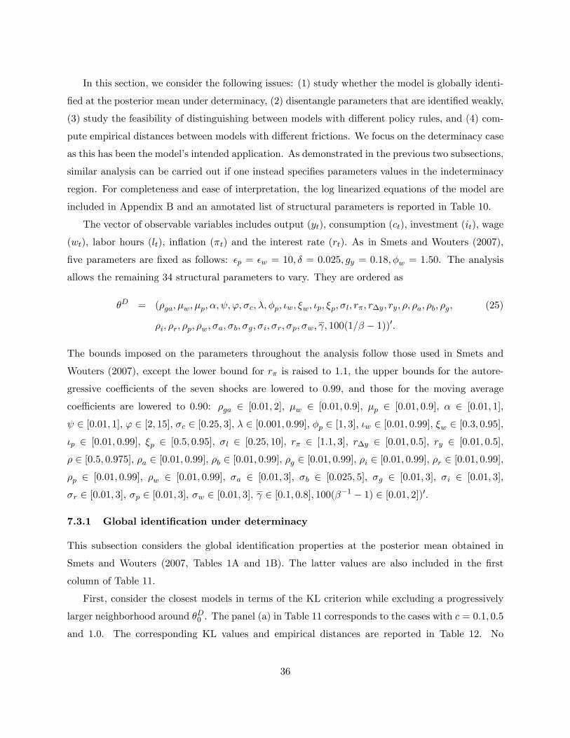
In this section, we consider the following issues: (1) study whether the model is globally identi-

�ed at the posterior mean under determinacy, (2) disentangle parameters that are identi�ed weakly,

(3) study the feasibility of distinguishing between models with di¤erent policy rules, and (4) com-

pute empirical distances between models with di¤erent frictions. We focus on the determinacy case

as this has been the model�s intended application. As demonstrated in the previous two subsections,

similar analysis can be carried out if one instead speci�es parameters values in the indeterminacy

region. For completeness and ease of interpretation, the log linearized equations of the model are

included in Appendix B and an annotated list of structural parameters is reported in Table 10.

The vector of observable variables includes output (yt), consumption (ct), investment (it); wage

(wt), labor hours (lt), in�ation (�t) and the interest rate (rt). As in Smets and Wouters (2007),

�ve parameters are �xed as follows: �p = �w = 10; � = 0:025; gy = 0:18; �w = 1:50. The analysis

allows the remaining 34 structural parameters to vary. They are ordered as

�D = (�ga; �w; �p; �; ; '; �c; �; �p; �w; �w; �p; �p; �l; r�; r�y; ry; �; �a; �b; �g; (25)

�i; �r; �p; �w; �a; �b; �g; �i; �r; �p; �w; ; 100(1=� � 1))0:

The bounds imposed on the parameters throughout the analysis follow those used in Smets and

Wouters (2007), except the lower bound for r� is raised to 1.1, the upper bounds for the autore-

gressive coe¢ cients of the seven shocks are lowered to 0.99, and those for the moving average

coe¢ cients are lowered to 0.90: �ga 2 [0:01; 2], �w 2 [0:01; 0:9], �p 2 [0:01; 0:9], � 2 [0:01; 1],

2 [0:01; 1], ' 2 [2; 15], �c 2 [0:25; 3], � 2 [0:001; 0:99], �p 2 [1; 3], �w 2 [0:01; 0:99], �w 2 [0:3; 0:95],�p 2 [0:01; 0:99], �p 2 [0:5; 0:95], �l 2 [0:25; 10], r� 2 [1:1; 3], r�y 2 [0:01; 0:5], ry 2 [0:01; 0:5],

� 2 [0:5; 0:975], �a 2 [0:01; 0:99], �b 2 [0:01; 0:99], �g 2 [0:01; 0:99], �i 2 [0:01; 0:99], �r 2 [0:01; 0:99],�p 2 [0:01; 0:99], �w 2 [0:01; 0:99], �a 2 [0:01; 3], �b 2 [0:025; 5], �g 2 [0:01; 3], �i 2 [0:01; 3],

�r 2 [0:01; 3], �p 2 [0:01; 3], �w 2 [0:01; 3], 2 [0:1; 0:8]; 100(��1 � 1) 2 [0:01; 2])0:

7.3.1 Global identi�cation under determinacy

This subsection considers the global identi�cation properties at the posterior mean obtained in

Smets and Wouters (2007, Tables 1A and 1B). The latter values are also included in the �rst

column of Table 11.

First, consider the closest models in terms of the KL criterion while excluding a progressively

larger neighborhood around �D0 . The panel (a) in Table 11 corresponds to the cases with c = 0:1; 0:5

and 1:0. The corresponding KL values and empirical distances are reported in Table 12. No

36

observationally equivalent model is found. This is a strong result, indicating that the Smets and

Wouters (2007) model is globally identi�ed at the posterior mean after �xing the �ve parameters.

Meanwhile, there exist models that are hard to distinguish from the original model even with c =

1:0. In that case, the empirical distances are 0:1159 and 0:3123 for T=150 and 1000. Interestingly,

for all values of c, the closest model is always found by moving the parameter corresponding to the

steady state elasticity of the capital adjustment cost function (').

Next, we repeat the analysis with ' �xed at 5:74. The parameters minimizing the KL criterion

are reported in Panel (b) in Table 11. For c = 0:1 and 0:5, the improvements are relatively small

with typical sample sizes. Substantial changes occur when c = 1:0. In addition, for all three cases,

the largest change is in the elasticity of labor supply (�l).

The above analysis shows that the model is globally identi�ed at the posterior mean after �xing

the �ve parameters. This is the �rst time such a strong statement about this model is made.

Also, it shows that among the behavioral parameters, ' and �l are identi�ed weakly. The latter

is consistent with the �nding of Smets and Wouters (2007, p. 594) obtained from a Bayesian

perspective.

7.3.2 Identi�cation of policy rules

The original model has the following monetary policy rule

rt = �rt�1 + (1� �) (r��t + ry (yt � y�t )) + r�y((yt � y�t )��yt�1 � y�t�1

�) + "rt : (26)

We consider replacing it by the following rule targeting expected rather than current in�ation:

rt = �rt�1 + (1� �) (r�E(�t+1) + ry (yt � y�t )) + r�y((yt � y�t )��yt�1 � y�t�1

�) + "rt :

The parameter vector minimizing the KL criterion equals (Here and below, the parameters are in

the same order as in (25).)

�D = (0:52; 0:80; 0:71; 0:18; 0:58; 5:45; 1:40; 0:70; 1:60; 0:55; 0:64; 0:27; 0:67; 1:35; 2:36; 0:22; 0:08;

0:80; 0:95; 0:22; 0:97; 0:72; 0:17; 0:90; 0:96; 0:45; 0:23; 0:53; 0:45; 0:25; 0:14; 0:24; 0:45; 0:01)0:

The resulting KL equals 0.0080.The empirical distance measures reported in Table 13 equal 0.4829

for T=150 and 0.9903 for T=1000. Therefore, unlike the previously considered small scale New

Keynesian models, here there is no (near) observational equivalence between the above two policy

rules.

37

Next, we consider two other policy rules. The �rst has the original output gap component

removed, i.e., ry = 0. The second has the output growth component shut o¤, i.e., r�y = 0. The

parameter vectors minimizing the respective KL criterion are

�D = (0:52; 0:79; 0:66; 0:17; 0:51; 7:98; 1:09; 0:80; 1:56; 0:57; 0:72; 0:24; 0:64; 2:41; 1:50; 0:19; 0:00;

0:72; 0:95; 0:19; 0:97; 0:68; 0:25; 0:89; 0:94; 0:46; 0:24; 0:53; 0:42; 0:24; 0:14; 0:24; 0:80; 0:01)0

and

�D = (0:47; 0:84; 0:73; 0:19; 0:53; 11:51; 1:24; 0:84; 1:72; 0:58; 0:74; 0:25; 0:64; 3:23; 1:52; 0:00; 0:04;

0:78; 0:96; 0:18; 0:97; 0:67; 0:09; 0:90; 0:96; 0:44; 0:25; 0:54; 0:42; 0:23; 0:14; 0:24; 0:24; 0:10)0

with the KL values equal to 0.0499 and 0.1334, respectively. Empirical distances reported in Table

13 show that both alternative models are distinguishable from the original one at �D0 even in small

samples. In the case of no output gap component, the empirical distance for the sample of 80

observations equals 0.7844 and reaches 0.9845 for samples of size 200. In case of shutting o¤ the

output growth component, the empirical distance already equals 0.9965 for the sample of size 80,

and equals 1 for T=150 and above.

We now examine whether there exists a parameter path along which the policy rules speci�ed

as (26) are (nearly) observationally equivalent as in the model of Lubik and Schorfheide (2004).

The curve in (7) is computed by changing only the �ve parameters in the Taylor rule. The results

are summarized in Table 14. There, the empirical distance rapidly increases along the curve. For

T=150, it reaches 0.9131 and 0.9510 along the two directions, where the corresponding Euclidean

distances from �D0 are only 0.0639 and 0.0718 respectively. This pattern is in sharp contrast with

that for Lubik and Schorfheide (2004). The result vividly illustrates how the identi�cation of the

policy parameters drastically changes when we move from small to medium scale DSGE models.

7.3.3 Identi�cation of frictions

This subsection examines how the dynamics of the model are a¤ected when the real and nominal

frictions are reduced substantially from their original values. The analysis parallels that of Smets

and Wouters (Section IV, Table 4) conducted from a Bayesian perspective. The relevant friction

parameters are �p (price stickiness), �w (wage stickiness), �p (price indexation), �w (wage index-

ation), ' (investment adjustment cost), � (habit persistence), (elasticity of capital utilization

adjustment cost), and �p (�xed costs in production). We change the parameters one at a time

38

to a value that e¤ectively dampens the e¤ect of the corresponding friction, and then search for

the model closest to the one at �D0 in terms of the KL criterion. Table 15 contains the resulting

parameter vectors, KL criteria and empirical distance measures.

First, consider the nominal frictions. Reducing the degree of nominal price and wage stickiness

to 0.10 results in an empirical distance of 1.00 for T=150 in both cases. This suggests that these

two frictions are very important for generating the dynamic properties of the model. A lower

price stickiness leads to a substantial increase in the degree of price indexation from 0.24 to 0.99.

Meanwhile, the price mark-up shock process becomes ampli�ed. It becomes more persistent (the

AR parameter changes from 0.89 to 0.97 and the MA parameter drops from 0.69 to 0.12), while

its error standard deviation also increases substantially (from 0.14 to 0.34). Turning to the wage

stickiness, reducing its level leads to an increase in the degree of wage indexation from 0.58 to

0.99. The wage mark-up becomes more persistent (the AR parameter changes from 0.96 to 0.98

and the MA parameter drops from 0.84 to 0.09) and its standard deviation increases substantially

(from 0.24 to 0.83). Interestingly, the investment adjustment cost parameter (') and labor supply

elasticity (�l) decrease substantially in both cases.

The price and wage indexation are relevant but less important, when compared with the Calvo

frictions, in generating the model�s dynamics. Reducing the price indexation to a very low level

of 0.01 leads to an empirical distance of 0.46 for T=150. Its KL value is also the smallest among

all cases that we consider. For both cases, leaving out either friction does not have any noticeable

impact on the other parameters.

Now consider the four real frictions. The results are summarized below. (1) Reducing the

elasticity of adjustment cost from 5.74 to 1.00 leads to an empirical distance of 1.00 for T=150.

The persistence and standard deviation of the investment shock process strongly increases. The

other parameters change relatively little. (2) Reducing habit formation in consumption from 0.71 to

0.10 also leads to an empirical distance of 1.00 for T=150. Here, the elasticity of capital utilization

adjustment cost ( ) increases, while the investment adjustment cost parameter (') and labor

supply elasticity (�l) both decrease substantially. Among the exogenous shocks, the investment

shock becomes more persistent and its standard deviation also increases. (3) Shutting down the

variable capital utilization results in the smallest KL criterion among the four, with an empirical

distance of 0.83 at T=150. All parameters remain roughly the same. (4) Finally, reducing the share

of �xed costs in production to 10 percent leads to an empirical distance of 1.00 for T=150. The

standard deviation of the technology shock increases and the process also becomes more persistent.

39

In summary, all four real frictions are important in generating the dynamic properties of the model

with the elasticity of capital utilization adjustment cost being the least so. The conclusions reached

regarding both the nominal and real frictions are consistent with the �ndings in Smets and Wouters

(2007) obtained from a Bayesian perspective.

7.3.4 Global identi�cation from business cycle frequencies

This subsection carries out analysis similar to that in Section 7.1.5. The �ndings can be summarized

as follows. First, the model is still globally identi�ed at �D0 when only business cycle frequencies are

considered. The respective parameter values minimizing the KL de�ned in (13) are broadly similar

to those in Table 11. These results mirror our �ndings for the two small scale models. Second,

distinguishing between alternative policy rules is still feasible at typical sample sizes. For T=80,

the distances at the minimizers of (13) are 0:1356; 0:2596; 0:8305 and for T=150, they grow to

0:1785; 0:3743; 0:9615 (these values can be contrasted with the second and the third rows in Table

13). This �nding is quite di¤erent from the two small scale models. It is notable that the changes

in empirical distances vary substantially across the policy rules. For the expected in�ation and the

output growth rules the empirical distances are more than halved compared to the full spectrum

case. In contrast, the empirical distances for the output gap rule change relatively little.

Finally, we also repeated the analysis summarized in Table 15 using business cycle frequencies.

The resulting empirical distances at the minimizers of (13) with T=80 in the same order as in the ta-

ble are (these can be compared with the second row in Table 15): 0:9461; 0:9370; 0:1090; 0:2222; 0:5895,

0:7662; 0:2433; 0:6661. Overall, the values imply that the statements made in the preceding sub-

section about the relative importance of various frictions also hold when con�ning attention to

the business cycle frequencies. Also, as in the case with monetary rules, the changes in empirical

distances vary substantially across frictions. The results for price and wage stickiness display very

little change, while those for price and wage indexation as well as for the variable capital utilization

fall dramatically to about a third of the respective values for the full spectrum. The empirical dis-

tances for the remaining real frictions decrease moderately. These �ndings are informative in view

of the fact that the current generation of DSGE models is designed for business cycle movements,

not �uctuations at very low or high frequencies.

40

8 Conclusion

This paper has presented a uni�ed framework for analyzing identi�cation in DSGE models that

encompasses both determinacy and indeterminacy. In addition to providing necessary and su¢ cient

conditions for local and global identi�cation, it also proposes a measure of the empirical distance

between DSGE models. Empirical illustrations for both small and medium scale models show that

the methods are informative and simple to implement. Although the analysis has focused on the

second order properties for the ease of exposition, the information from the steady states can be

easily incorporated. The results obtained are also applicable to other dynamic models with well

de�ned spectra, such as (factor augmented) vector autoregressive moving average models.

41

References

Altug, S. (1989): �Time-to-Build and Aggregate Fluctuations: Some New Evidence,� Interna-

tional Economic Review, 30, 889�920.

An, S., and F. Schorfheide (2007): �Bayesian Analysis of DSGE Models,�Econometric Re-

views, 26, 113�172.

Arellano, M., L. P. Hansen, and E. Sentana (2012): �Underidenti�cation?,� Journal of

Econometrics, 170, 256�280.

Benati, L., and P. Surico (2009): �VAR Analysis and the Great Moderation,� American

Economic Review, 99, 1636�1652.

Benhabib, J., and R. E. A. Farmer (1999): �Indeterminacy and Sunspots in Macroeconomics,�

The Handbook of Macroeconomics, 1, 387�448.

Benhabib, J., S. Schmitt-Grohé, and M. Uribe (2001): �Monetary Policy and Multiple

Equilibria,�American Economic Review, 91, 167�186.

Beyer, A., and R. E. A. Farmer (2004): �On the Indeterminacy of New-Keynesian Eco-

nomics,�European Central Bank Working Paper 323.

Blanchard, O. (1982): �Identi�cation in Dynamic Linear Models with Rational Expectations,�

NBER Technical Working Paper 0024.

Boivin, J., and M. P. Giannoni (2006): �Has Monetary Policy Become More E¤ective?,�The

Review of Economics and Statistics, 88, 445�462.

Brillinger, D. R. (2001): Time Series: Data Analysis and Theory. SIAM.

Brockwell, P., and R. Davis (1991): Time Series: Theory and Methods. New York: Springer-

Verlag, 2 edn.

Canova, F., F. Ferroni, and C. Matthes (2013): �Choosing the Variables to Estimate Sin-

gular DSGE Models,�Forthcoming in Journal of Applied Econometrics.

42

Canova, F., and L. Sala (2009): �Back to Square One: Identi�cation Issues in DSGE Models,�

Journal of Monetary Economics, 56, 431�449.

Chernoff, H. (1952): �Measure of Asymptotic E¢ ciency for Tests of a Hypothesis Based on the

Sum of Observations,�Annals of Mathematical Statistics, 23, 493�507.

Christiano, L. J., M. Eichenbaum, and D. Marshall (1991): �The Permanent Income

Hypothesis Revisited,�Econometrica, 59, 397�423.

Christiano, L. J., and R. J. Vigfusson (2003): �Maximum Likelihood in the Frequency

Domain: the Importance of Time-to-plan,�Journal of Monetary Economics, 50, 789�815.

Clarida, R., J. Galí, and M. Gertler (2000): �Monetary Policy Rules and Macroeconomic

Stability: Evidence and Some Theory,�The Quarterly Journal of Economics, 115, 147�180.

Cochrane, J. H. (2011): �Determinacy and Identi�cation with Taylor Rules,�Journal of Polit-

ical Economy, 119, 565�615.

(2014): �The New-Keynesian Liquidity Trap,�Unpublished Manuscript.

Cox, D. R. (1961): �Tests of Separate Families of Hypotheses,�in Proceedings of the 4th Berkeley

Symposium in Mathematical Statistics and Probability, vol. 1, pp. 105�123. Berkeley: University of

California Press.

Del Negro, M., F. X. Diebold, and F. Schorfheide (2008): �Priors from Frequency-Domain

Dummy Observations,�No. 310 in 2008 Meeting Papers. Society for Economic Dynamics.

Del Negro, M., and F. Schorfheide (2008): �Forming Priors for DSGE Models (and How it

A¤ects the Assessment of Nominal Rigidities),�Journal of Monetary Economics, 55, 1191�1208.

Diebold, F. X., L. E. Ohanian, and J. Berkowitz (1998): �Dynamic Equilibrium Economies:

A Framework for Comparing Models and Data,�The Review of Economic Studies, 65, 433�451.

Fernández-Villaverde, J., and J. F. Rubio-Ramírez (2004): �Comparing Dynamic Equi-

librium Models to Data: a Bayesian Approach,�Journal of Econometrics, 123, 153�187.

FukaµC, M., D. F. Waggoner, and T. Zha (2007): �Local and Global Identi�cation of DSGE

Models: A Simultaneous-Equation Approach,�Working paper.

43

Guerron-Quintana, P. A. (2010): �What You Match Does Matter: The E¤ects of Data on

DSGE Estimation,�Journal of Applied Econometrics, 25, 774�804.

Haavelmo, T. (1944): �The Probability Approach in Econometrics,�Econometrica, 12, supple-

ment, 1�118.

Hannan, E. J. (1970): Multiple Time Series. New York: John Wiley.

Hansen, L. P. (2007): �Beliefs, Doubts and Learning: Valuing Macroeconomic Risk,�American


Hansen, L. P., and T. J. Sargent (1993): �Seasonality and Approximation Errors in Rational

Expectations Models,�Journal of Econometrics, 55, 21�55.

Iskrev, N. (2010): �Local Identi�cation in DSGE Models,�Journal of Monetary Economics, 57,

189�202.

Komunjer, I., and S. Ng (2011): �Dynamic Identi�cation of Dynamic Stochastic General Equi-

librium Models,�Econometrica, 79, 1995�2032.

Koopmans, T. C. (1949): �Identi�cation Problems in Economic Model Construction,�Econo-

metrica, 2, 125�144.

Leeper, E. M. (1991): �Equilibria Under �Active�and �Passive�Monetary and Fiscal Policies,�

Journal of Monetary Economics, 27, 129�147.

Lubik, T., and F. Schorfheide (2003): �Computing Sunspot Equilibria in Linear Rational

Expectations Models,�Journal of Economic Dynamics and Control, 28, 273�285.

(2004): �Testing for Indeterminacy: An Application to U.S. Monetary Policy,�American


Mavroeidis, S. (2010): �Monetary Policy Rules and Macroeconomic Stability: Some New Evi-

dence,�American Economic Review, 100, 491�503.

Parzen, E. (1983): �Autoregressive Spectral Estimation,� in Handbook of Statistics, ed. by

D. Brillinger, and P. Krishnaiah, vol. III, pp. 221�247. Amsterdam: North Holland.

Pesaran, H. (1981): �Identi�cation of Rational Expectations Models,�Journal of Econometrics,

16, 375�398.

44

Pinsker, M. S. (1964): Information and Information Stability of Random Variables and

Processes. San-Francisco: Holden-Day.

Qu, Z., and D. Tkachenko (2012): �Identi�cation and Frequency Domain Quasi-maximum

Likelihood Estimation of Linearized Dynamic Stochastic General Equilibrium Models,�Quantita-

tive Economics, 3, 95�132.

Rothenberg, T. J. (1971): �Identi�cation in Parametric Models,�Econometrica, 39, 577�591.

Rubio-Ramírez, J. F., D. F. Waggoner, and T. Zha (2010): �Structural Vector Autore-

gressions: Theory of Identi�cation and Algorithms for Inference,�Review of Economic Studies, 77,

665�696.

Sims, C. A. (1993): �Rational Expectations Modeling with Seasonally Adjusted Data,�Journal

of Econometrics, 55, 9�19.

(2002): �Solving Linear Rational Expectations Models,�Computational Economics, 20,

1�20.

Smets, F., and R. Wouters (2003): �An Estimated Dynamic Stochastic General Equilibrium

Model of the Euro Area,�Journal of the European Economic Association, 1, 1123�1175.

(2007): �Shocks and Frictions in US Business Cycles: A Bayesian DSGE Approach,�

The American Economic Review, 97, 586�606.

Tkachenko, D., and Z. Qu (2012): �Frequency Domain Analysis of Medium Scale DSGE

Models with Application to Smets and Wouters (2007),�Advances in Econometrics, 28, 319�385.

Wallis, K. F. (1980): �Econometric Implications of the Rational Expectations Hypothesis,�

Econometrica, 48, 49�73.

Watson, M. W. (1993): �Measures of Fit for Calibrated Models,�Journal of Political Economy,

101, 1011�1041.

45

Appendix A. Model Solution under Indeterminacy

This appendix contains an alternative derivation of Lubik and Schorfheide�s (2003) representa-tion for the full set of stable solutions under indeterminacy. It also contains a normalization basedon the reduced column echelon form when the degree of indeterminacy exceeds one.

The system (1) can be transformed using a QZ decomposition, i.e., there exist matrices Q;Z;�and such that

Q��Z� = �0;

Q�Z� = �1;

where Q and Z are unitary, � and are upper triangular. Let wt=Z�St and premultiply (1) by Q:24 �11 �12

0 �22

3524 w1;t

w2;t

35 =24 11 12

0 22

3524 w1;t�1

w2;t�1

35+24 Q1:

Q2:

35 ("t +��t) ; (A.1)

where an ordering has been imposed such that the diagonal elements of �11 (�22) are greater(smaller) than those of 11 (22) in absolute values; the matrix Q is partitioned into Q1: and Q2:.Then, because the generalized eigenvalues corresponding to the pair �22 and 22 are unstable and"t and �t are serially uncorrelated, the block of equations corresponding to w2;t has a stable solutionif and only if w2;0 = 0 and

Q2:��t = �Q2:"t for all t > 0: (A.2)

The condition (A.2) determines Q2:��t as a function of "t. However, it may be insu¢ cient todetermine Q1:��t, in which case it will lead to indeterminacy.

Since the rows of Q2:� can be linearly dependent, Sims (2002) and Lubik and Schorfheide (2003)suggested to work with its singular value decomposition to isolate the e¤ective restrictions imposedon �t. This leads to

Q2:� = [ U:1 U:2 ]

24 D11 0

0 0

3524 V �:1

V �:2

35 = U:1D11V�:1; (A.3)

where [ U:1 U:2 ] and [ V:1 V:2 ] are unitary matrices and D11 is nonsingular. The submatrices

U:1 and V �:1 are unique up to multiplication by a unit-phase factor exp(i') (for the real case, up tosign). The spaces spanned by U:2 and V:2 are also unique, although the matrices themselves are notif their column dimensions exceed one. In the latter case, as a normalization, we use the reducedcolumn echelon form for V:2 when implementing the relevant procedures.4

4Note that matrices with the same column space have the same unique reduced column echelon form. To see this,suppose eV:2 and �V:2 are two di¤erent choices of V:2 in the singular value decomposition of Q2:�. Because they spanthe same column space, they must satisfy eV:2 = �V:2N (A.4)

with N being a nonsingular matrix. Let eV R:2 be the unique reduced column echelon form of eV:2. Then, by de�nition,

there exists a sequence of elementary matrices E1; :::; EK such that eV R:2 = eV:2E1 � � � EK . Thus, using (A.4), eV R

:2 =�V:2NE1 � � � EK . Further, the matrix N itself equals the product of elementary matrices because it is nonsingular.Therefore, eV R

:2 is also the unique reduced column echelon form of �V:2.

A-1

Applying (A.3), (A.2) can be equivalently represented as

U:1D11V�:1�t = �Q2:"t for all t > 0: (A.5)

Premultiplying (A.5) by the conjugate transpose of [ U:1 U:2 ] does not alter the restrictions

because the latter is nonsingular. Thus, (A.5) is equivalent to (using U�:1U:1 = I and U�:2U:1 = 0)24 D11V�:1�t

0

35 =24 �U�:1Q2:"t�U�:2Q2:"t

35 for all t > 0:

The second block of equations places no restrictions on �t. The �rst block is equivalent to

V �:1�t = �D�111 U

�:1Q2:"t:

This can be viewed as a system of linear equations of the form Ax = b with A = V �:1 and b =�D�1

11 U�:1Q2:"t. The full set of solutions for such a system is given by

fp+ v : v is any solution to Ax = 0 and p is a speci�c solution to Ax = bg: (A.6)

Here, a speci�c solution is given by p = �V:1D�111 U

�:1Q2:"t while �t solves V

�:1�t = 0 if and only if

�t = V:2�t with �t being an arbitrary vector conformable with V:2. Therefore, the full set of solutionsto (A.5) can be represented as�

�t : �t = �V:1D�111 U

�:1Q2:"t + V:2�t with Et�1�t = 0

: (A.7)

The restriction Et�1�t = 0 follows because �t is an expectation error and Et�1"t = 0. Thisrepresentation is the same as in Proposition 1 in Lubik and Schorfheide (2003). It allows fordeterminacy as a special case.

We now provide some computational details on how to use (A.7) to solve for St in (1) as in Sims(2002). De�ne a matrix � as the projection coe¢ cients of the rows of Q1:� onto those of Q2:�:

� = Q1:�V:1D�111 U

�:1:

Note that Q1:��Q2:� = Q1:��Q1:�V:1V �:1 = Q1:�(I � V:1V �:1), which equals zero under deter-minacy. Multiplying (A.1) by 24 I ��

0 I

35leads to24 �11 �12 � ��22

0 �22

3524 w1;t

w2;t

35 =24 11 12 � �22

0 22

3524 w1;t�1

w2;t�1

35+24 Q1: � �Q2:

Q2:

35 ("t +��t) :

A-2

Imposing the restrictions (A.2), the above system reduces to24 �11 �12 � ��220 I

3524 w1;t

w2;t

35 =24 11 12 � �22

0 0

3524 w1;t�1

w2;t�1

35+24 Q1: � �Q2:

0

35 ("t +��t) :Further, using the expression (A.7),

(Q1: � �Q2:)��t = (Q1:�� Q2:�)��V:1D�1

11 U�:1Q2:"t + V:2�t

�= �Q1:�(I � V:1V �:1)V:1D�1

11 U�:1Q2:"t +Q1:�(I � V:1V �:1)V:2�t:

The �rst term on the right hand side equals zero. Therefore24 �11 �12 � ��220 I

3524 w1;t

w2;t

35 =

24 11 12 � �220 0

3524 w1;t�1

w2;t�1

35+24 Q1: � �Q2:

0

35"t+

24 Q1:�(I � V:1V �:1)

0

35V:2�t:Call the most left hand side matrix G0. Multiply both sides of the equation by ZG�10 and usewt = Z�St, then

St = �1St�1 +�""t +��t;

where

�1 = ZG�10

24 11 12 � �220 0

35Z�;�" = ZG�10

24 Q1: � �Q2:0

35;�� = ZG�10

24 Q1:�(I � V:1V �:1)

0

35V:2:Because

G�10 =

24 ��111 ��111 (�12 � ��22)

0 I

35 ;the above matrices can be equivalently represented as �1 = Z:1�

�111 [ 11 12 � �22 ]Z�, �" =

Z:1��111 (Q1: � �Q2:) and �� = Z:1�

�111 Q1:�(I � V:1V �:1)V:2, where Z:1 includes the �rst block of

columns of Z conformable with �11.

A-3

Appendix B. The Equations and Parameters of the Smets and Wouters (2007) Model

The model has seven observable endogenous variables with seven exogenous shocks. Below isan outline of the log linearized system. They are consistent with Smets and Wouters�(2007) code.

The aggregate resource constraint: It satis�es

yt = cyct + iyit + zyzt + "gt :

Output (yt) is composed of consumption (ct), investment (it), capital utilization costs as a functionof the capital utilization rate (zt), and exogenous spending ("

gt ). The latter follows an AR(1) model

with an i.i.d. Normal error term (�gt ); and is also a¤ected by the productivity shock (�at ) as follows:

"gt = �g"gt�1 + �ga�

at + �

gt :

The coe¢ cients cy; iy and zy are functions of the steady state spending-output ratio (gy), steadystate output growth ( ), capital depreciation (�), household discount factor (�); intertemporalelasticity of substitution (�c), �xed costs in production (�p), and share of capital in production (�):iy = ( �1+�)ky; cy = 1�gy� iy; and zy = Rk�ky. Here, ky is the steady state capital-output ratio,and Rk� is the steady state rental rate of capital: ky = �p (L�=k�)

��1 = �p�((1� �)=�)

�Rk�=w�

��1with w� =

��(1� �)(1��)=[�p

�Rk��]�1=(1��)

, and Rk� = ��1 �c � (1� �):

Households: The consumption Euler equation is

ct = c1ct�1 + (1� c1)Etct+1 + c2(lt � Etlt+1)� c3(rt � Et�t+1)� "bt : (B.1)

where lt is hours worked, rt is the nominal interest rate, and �t is in�ation. The disturbance "btfollows

"bt = �b"bt�1 + �

bt :

The relationship of the coe¢ cients in (B.1) to the habit persistence (�), steady state labor marketmark-up (�w), and other structural parameters highlighted above is

c1 =�=

1 + �= ; c2 =

(�c � 1)�wh�L�=c�

��c (1 + �= )

; c3 =1� �=

(1 + �= )�c;

wherewh�L�=c� =

1

�w

1� ��

Rk�ky1

cy;

where Rk� and ky are de�ned as above, and cy = 1� gy � ( � 1 + �)ky:The dynamics of households�investment are given by

it = i1it�1 + (1� i1)Eti+1 + i2qt + "it;

B-1

where "it is a disturbance to the investment speci�c technology process, given by

"it = �i"it�1 + �

it:

The coe¢ cients satisfy

i1 =1

1 + � (1��c); i2 =

1�1 + � (1��c)

� 2'

;

where ' is the steady state elasticity of the capital adjustment cost function. The correspondingarbitrage equation for the value of capital is given by

qt = q1Etqt+1 + (1� q1)Etrkt+1 � (rt � Et�t+1)�1

c3"bt , (B.2)

with q1 = � ��c (1� �) = (1� �)=(Rk� + 1� �):

Final and intermediate goods market: The aggregate production function is

yt = �p (�kst + (1� �) lt + "at ) ;

where � captures the share of capital in production, and the parameter �p is one plus the �xedcosts in production. Total factor productivity follows the AR(1) process

"at = �a"at�1 + �

at :

The current capital service usage (kst ) is a function of capital installed in the previous period (kt�1)and the degree of capital utilization (zt):

kst = kt�1 + zt:

Furthermore, the capital utilization is a positive fraction of the rental rate of capital (rkt ):

zt = z1rkt ; where z1 = (1� )= ;

and is a positive function of the elasticity of the capital utilization adjustment cost function andnormalized to be between zero and one. The accumulation of installed capital (kt) satis�es

kt = k1kt�1 + (1� k1) it + k2"it;

where "it is the investment speci�c technology process as de�ned before, and k1 and k2 satisfy

k1 =1� � , k2 =

�1� 1� �

��1 + � (1��c)

� 2':

The price mark-up satis�es�pt = � (kst � lt) + "at � wt;

B-2

where wt is the real wage. The New Keynesian Phillips curve is

�t = �1�t�1 + �2Et�t+1 � �3�pt + "pt ;

where "pt is a disturbance to the price mark-up, following the ARMA(1,1) process given by

"pt = �p"pt�1 + �

pt � �p�

pt�1:

The MA(1) term is intended to pick up some of the high frequency �uctuations in prices. ThePhillips curve coe¢ cients depend on price indexation (�p) and stickiness (�p), the curvature of thegoods market Kimball aggregator ("p), and other structural parameters:

�1 =�p

1 + � (1��c)�p; �2 =

� (1��c)

1 + � (1��c)�p; �3 =

1

1 + � (1��c)�p

�1� � (1��c)�p

� �1� �p

��p��p � 1

�"p + 1

� :

Finally, cost minimization by �rms implies that the rental rate of capital satis�es

rkt = � (kst � lt) + wt:

Labor market: The wage mark-up is

�wt = wt ��llt +

1

1� �= (ct � (�= )ct�1)�;

where �l is the elasticity of labor supply. Real wage wt adjusts slowly according to

wt = w1wt�1 + (1� w1) (Etwt+1 + Et�t+1)� w2�t + w3�t�1 � w4�wt + "wt ;

where the coe¢ cients are functions of wage indexation (�w) and stickiness (�w) parameters, andthe curvature of the labor market Kimball aggregator ("w):

w1 =1

1 + � (1��c); w2 =

1 + � (1��c)�w1 + � (1��c)

; w3 =�w

1 + � (1��c);

w4 =1

1 + � (1��c)

�1� � (1��c)�w

�(1� �w)

�w ((�w � 1) "w + 1):

The wage mark-up disturbance follows an ARMA(1,1) process:

"wt = �w"wt�1 + �

wt � �w�wt�1:

Monetary policy: The empirical monetary policy reaction function is

rt = �rt�1 + (1� �) (r��t + ry (yt � y�t )) + r�y((yt � y�t )��yt�1 � y�t�1

�) + "rt :

The monetary shock "rt follows an AR(1) process:

"rt = �r"rt�1 + �

rt :

The variable y�t stands for the time-varying optimal output level that is the result of a �exibleprice-wage economy. Since the equations for the �exible price-wage economy are essentially thesame as above, but with the variables �pt and �

wt set to zero, we omit the details.

B-3

Appendix C. Proofs

The proofs for Theorem 1 and Corollary 1 are essentially the same as those for Theorem 1and Corollary 3 in Qu and Tkachenko (2012, supplementary appendix). This is because, after theparameter augmentation, � determines the second order properties of the process. Here we stillinclude the full detail to make the paper self-contained.

Let

f�(!)R =

24 Re(f�(!)) Im(f�(!))

� Im(f�(!)) Re(f�(!))

35 , (C.1)

where Re() and Im() denote the real and the imaginary parts of a complex matrix, i.e., if C = A+Bi,then Re(C) = A and Im(C) = B. Because f�(!) is Hermitian, f�(!)R is real and symmetric (seeLemma 3.7.1(v) in Brillinger, 2001). Further, let

R(!; �) = vec(f�(!)R):

Because the correspondence between f�(!) and R(!; �) is one to one, to prove the results it su¢ cesto consider R(!; �). In addition, Lemma A1 in Qu and Tkachenko (2012, supplementary material)states that �

@ vec f�(!)

@�0

��@ vec f�(!)@�0

�=1

2

�@R(!; �)

@�0

�0�@R(!; �)@�0

�: (C.2)

This implies that the left hand side, therefore G(�), is real, symmetric and positive semide�nite.Proof of Theorem 1. The relationship (C.2) implies that G(�) equals

1

2

Z �

��

�@R(!; �0)

@�0

�0�@R(!; �0)@�0

�d!:

This allows us to adopt the arguments in Theorem 1 in Rothenberg (1971) to prove the result.Suppose �0 is not locally identi�ed. Then, there exists an in�nite sequence of vectors f�kg1k=1

approaching �0 such that, for each k,

R(!; �0) = R(!; �k) for all ! 2 [��; �] .

For an arbitrary ! 2 [��; �], by the mean value theorem and the di¤erentiability of f�(!) in �;

0 = Rj(!; �k)�Rj(!; �0) =@Rj(!;e�(j; !))

@�0(�k � �0);

where the subscript j denotes the j-th element of the vector and e�(j; !) lies between �k and �0 andin general depends on both ! and j. Let

dk = (�k � �0)= k�k � �0k ;

then@Rj(!;e�(j; !))

@�0dk = 0 for every k.

C-1

The sequence fdkg lies on the unit sphere and therefore it has a convergent subsequence with a limitpoint d (note that d does not depend on j or !). Assume fdkg itself is the convergent subsequence.As �k ! �0; dk approaches d and

limk!1

@Rj(!;e�(j; !))@�0

dk =@Rj(!; �0)

@�0d = 0;

where the convergence result holds because f�(!) is continuously di¤erentiable in �. Because thisholds for an arbitrary j, it holds for the full vector R(!; �0): Therefore

@R(!; �0)

@�0d = 0;

which implies

d0�@R(!; �0)

@�0

�0�@R(!; �0)@�0

�d = 0:

Because the above result holds for an arbitrary ! 2 [��; �]; it also holds when integrating over[��; �]: Thus

d0�Z �

��

�@R(!; �0)

@�0

�0�@R(!; �0)@�0

�d!

�d = 0:

Because d 6= 0, G(�0) is singular.To show the converse, suppose that G(�) has a constant reduced rank in a neighborhood of

�0 denoted by �(�0). Then, consider the characteristic vector c(�) associated with one of the zeroroots of G(�). Because Z �

��

�@R(!; �)

@�0

�0�@R(!; �)@�0

�d! � c(�) = 0;

we have Z �

��

�@R(!; �)

@�0c(�)

�0�@R(!; �)@�0

c(�)

�d! = 0:

Since the integrand is continuous in ! and always non-negative, we must have�@R(!; �)

@�0c(�)

�0�@R(!; �)@�0

c(�)

�= 0

for all ! 2 [��; �] and all � 2 �(�0). Furthermore, this implies

@R(!; �)

@�0c(�) = 0 (C.3)

for all ! 2 [��; �] and all � 2 �(�0). Because G(�) is continuous and has a constant rank in �(�0),the vector c(�) is continuous in �(�0). Consider the curve � de�ned by the function �(v) whichsolves for 0� v � �v the di¤erential equation

@�(v)

@v= c(�);

�(0) = �0:

C-2

Then,@R(!; �(v))

@v=@R(!; �(v))

@�(v)0@�(v)

@v=@R(!; �(v))

@�(v)0c(�) = 0 (C.4)

for all ! 2 [��; �] and 0 � v � �v, where the last equality uses (C.3). Thus, R(!; �) is constanton the curve �. This implies that f�(!) is constant on the same curve and that �0 is locallyunidenti�able. This completes the proof.Proof of Corollary 1. Recall � = (�D0; �U 0)

0. Suppose �D0 is not locally identi�ed. Then, there

exists an in�nite sequence of vectors f�kg1k=1 approaching �0 such that

R(!; �0) = R(!; �k) for all ! 2 [��; �] and each k.

By the de�nition of the partial identi�cation,��Dkcan be chosen such that

�Dk � �D0 = k�k � �0k >" with " being some arbitrarily small positive number. The values of �Uk can either change or stay�xed in this sequence; no restrictions are imposed on them besides those in the preceding display.As in the proof of Theorem 1, in the limit, we have

@R(!; �0)

@�0d = 0;

with dD 6= 0 (where dD is comprised of the elements in d that correspond to �D). Therefore, onone hand,

G(�0)d = 0;

on the other hand, because dD 6= 0 and, by de�nition, @�D0 =@�0 = [Idim(�D); 0dim(�U )], we have

@�D0@�0

d = dD 6= 0;

which impliesGa(�0)d 6= 0:

Thus, we have identi�ed a vector that falls into the orthogonal column space of G(�0) but not ofGa(�0): Because the former orthogonal space always includes the latter as a subspace, this resultimplies that Ga(�0) has a higher column rank than G(�0).

To show the converse, suppose that G(�) and Ga(�) have constant ranks in a neighborhood of�0 denoted by �(�0). Because the rank of G(�) is lower than that of Ga(�); there exists a vectorc(�) such that

G(�)c(�) = 0 but Ga(�)c(�) 6= 0;

which implies for all ! 2 [��; �] and all � 2 �(�0) (see arguments leading to (C.3))

@R(!; �)

@�0c(�) = 0;

but 24 @R(!; �)=@�0

@�D=@�0

35 c(�) =24 0

cD(�)

35 6= 0;C-3

where cD(�) denotes the elements in c(�) that correspond to �D. Because G(�) is continuous andhas constant rank in �(�0), the vector c(�) is continuous in �(�0). As in Theorem 1, consider thecurve � de�ned by the function �(v) which solves for 0� v � �v the di¤erential equation

@�(v)

@v= c(�); �(0) = �0:

On one hand, because cD(�) 6= 0 and cD(�) is continuous in �; points on this curve correspond todi¤erent �D: On the other hand,

@R(!; �(v))

@v=@R(!; �(v))

@�(v)0@�(v)

@v=@R(!; �(v))

@�(v)0c(�) = 0

for all ! 2 [��; �] and 0 � v � �v; implying f�(!) is constant on the same curve. Therefore, �D0 isnot locally partially identi�able.Proof of Theorem 2. First, for any ! 2 [��; �], f�1�1 (!)f�0(!) admits an eigenvalue decomposi-tion and all the eigenvalues are strictly positive. This can be shown as follows. Because f�1(!) andf�0(!) are positive de�nite, they have well de�ned Cholesky decompositions

f�1(!) = A�(!)A(!);

f�0(!) = B�(!)B(!):

Therefore,f�1�1 (!)f�0(!) = A(!)�1A�(!)�1B�(!)B(!):

Pre and post multiplying both sides by A(!) and A(!)�1 yields

A(!)f�1�1 (!)f�0(!)A(!)�1 =

�B(!)A(!)�1

�� B(!)A(!)�1

�:

The right hand side is a positive de�nite matrix. It has a well de�ned eigen decomposition withstrictly positive eigenvalues. Because the above pre and post multiplication does not a¤ect theeigenvalues, it follows that f�1�1 (!)f�0(!) also has an eigenvalue decomposition with strictly positiveeigenvalues. This in turn implies that f�1�1 (!)f�0(!) is Hermitian.

Write the eigenvalue decomposition of f�1�1 (!)f�0(!) as

f�1�1 (!)f�0(!) = V �(!)�(!)V (!); (C.5)

where all the eigenvalues in �(!) are real and strictly positive. Let �j(!) be the j-th largesteigenvalue, then

1

2

ntr(f�1�1 (!)f�0(!))� log det(f

�1�1(!)f�0(!))� nY

o=

1

2

nYXj=1

[�j(!)� log �j(!)� 1] :

C-4

For arbitrary �j(!) > 0, we always have �j(!)� log �j(!)� 1 � 0 with the equality holding if andonly if �j(!) = 1. Integrating over [��; �], we obtain KL(�0; �1) � 0 with the equality holding ifand only if �(!)= I for all ! 2 [��; �]. However, using (C.5), the latter is equivalent to

f�1�1 (!)f�0(!) = V �(!)V (!) = I

for all ! 2 [��; �]. This is further equivalent to f�1(!) = f�0(!) for all ! 2 [��; �].Proof of Theorem 3. We only establish the limiting distribution under the null hypothesis asthe proof under the alternative hypothesis is similar. First, from Assumption 5 and the Lipschitzcondition in Assumption 6,

T 1=2

0@ 1

2T

T�1Xj=1

nlog det(h�1�0 (!j)f�0(!j))� tr(h

�1�0(!j)f�0(!j)) + nY

o+KLfh(�0; �0)

1A= O

�T��+1=2

�= o(1):

Second,

1

2T 1=2

T�1Xj=1

trn�f�1�0 (!j)� h

�1�0(!j)

�(I(!j)� f�0(!j))

o(C.6)

=1

2T 1=2

T�1Xj=1

vecnf�1�0 (!j)� h

�1�0(!j)

o�vec fI(!j)� f�0(!j)g :

This satis�es a multivariate central limit theorem under the assumptions stated in the theorem.The limiting variance is given by

limT!1

1

2T

T�1Xj=1

vecnf�1�0 (!j)� h

�1�0(!j)

o� �f�0(!j)

0 f�0(!j)�vecnf�1�0 (!j)� h

�1�0(!j)

o=

1

4�

Z �

��trnhI � f�0(!)h�1�0 (!)

i hI � f�0(!)h�1�0 (!)

iod!:

Under the alternative hypothesis, the same argument can be applied. This completes the proof.Proof of Corollary 6. Relaxing the cumulant condition does not a¤ect the asymptotic normality.Therefore, it su¢ ces to verify that the asymptotic variances have the stated expressions. Weonly consider the null hypothesis as the proof under the alternative hypothesis is similar. Let�(!) = f�1�0 (!j)� h

�1�0(!j). Then, (C.6) can be written as

1

2T 1=2

T�1Xj=1

tr f�(!j)(I(!j)� f�0(!j))g =nYXk;l=1

8<: 1

2T 1=2

T�1Xj=1

�kl(!j)(Ilk (!j)� f�0lk(!j))

9=; ;

where �kl(!j) is the (k; l)-th element of �(!j) and other quantities are de�ned analogously. Denotethe quantity in the curly brackets by A(k; l). Applying the same argument as in Proposition 10.8.5

C-5

in Brockwell and Davis (1991), we have

A(k; l) =1

2T 1=2

T�1Xj=1

dim(e"t)Xa;b=1

�kl(!j)Hla(!j)�Ie"ab (!j)� EIe"ab (!j)

�H�bk(!j) + op(1);

where Ie"ab (!j) denotes the (a; b)-th element of the periodogram of e"t and H�bk(!j) is the (b; k)-th

element of H�(!j). Note that H�bk(!j) = Hkb(!j). The covariance between A(k; l) and A(m;n)

then equals

1

4T

T�1Xj:h=1

dim(e"t)Xa;b;c;d=1

�kl(!j)Hla(!j)H�bk(!j) Cov(I

e"ab (!j) ; I

e"cd (!h))�mn(!h)Hnc(!h)H

�dm(!h) + o(1)

=1

4T

T�1Xj;h=1

dim(e"t)Xa;b;c;d=1

�kl(!j)Hla(!j)H�bk(!j) Cov(I

e"ab (!j) ; I

e"cd (!h))�nm(!h)H

�cn(!h)Hmd(!h) + o(1):

Proposition 11.7.3 in Brockwell and Davis (1991) shows for 0 < !j ; !h < �:

Cov�Ie"ab (!j) ; Ie"cd (!h)

�=

8<: 14�2T

�abcd +14�2

�ac�db

14�2T

�abcd

if !j = !h;

if !j 6= !h,

where �ac is the covariance between the a-th and the c-th elements of e"t. Applying this result, thepreceding summation equals

1

8�2T

T�1Xj=1

8<:dim(e"t)Xa;c=1

�kl(!j)Hla(!j)�acH�cn(!j)

dim(e"t)Xb;d=1

�nm(!j)Hmd(!j)�dbH�bk(!j)

9=;+

1

16�2T 2

dim(e"t)Xa;b;c;d=1

�abcd

24T�1Xj=1

H�bk(!j)�kl(!j)Hla(!j)

T�1Xh=1

H�cn(!h)�nm(!h)Hmd(!h)

35+ o(1):The �rst term converges to

1

4�

Z �

��kl(!)f�0ln(!)�nm(!)f�0mk(!)d!:

Upon taking summation over 1� k; l;m; n � nY , it equals

1

4�

Z �

��trn�f�1�0 (!)� h

�1�0(!)�f�0(!)

�f�1�0 (!)� h

�1�0(!)�f�0(!)

od!

=1

4�

Z �

��trnhI � f�0(!)h�1�0 (!)

i hI � f�0(!)h�1�0 (!)

iod!:

C-6

Meanwhile, the second term summed over 1� k; l;m; n � nY equals

1

16�2T 2

dim(e"t)Xa;b;c;d=1

�abcd

24T�1Xj=1

nYXk;l=1

H�bk(!j)�kl(!j)Hla(!j)

T�1Xh=1

nYXm;n=1

H�cn(!h)�nm(!h)Hmd(!h)

35! 1

16�2

dim(e"t)Xa;b;c;d=1

�abcd

�1

2�

Z �

��H�(!)

�f�1�0 (!)� h

�1�0(!)�H(!)d!

�ba

��1

2�

Z �

��H�(!)

�f�1�0 (!)� h

�1�0(!)�H(!)d!

�cd

:

Because �abcd = �bacd, the right hand side can also be expressed as

1

16�2

dim(e"t)Xa;b;c;d=1

�abcd

�1

2�

Z �

��H�(!)

�f�1�0 (!)� h

�1�0(!)�H(!)d!

�ab

��1

2�

Z �

��H�(!)

�f�1�0 (!)� h

�1�0(!)�H(!)d!

�cd

:

This completes the proof.

C-7

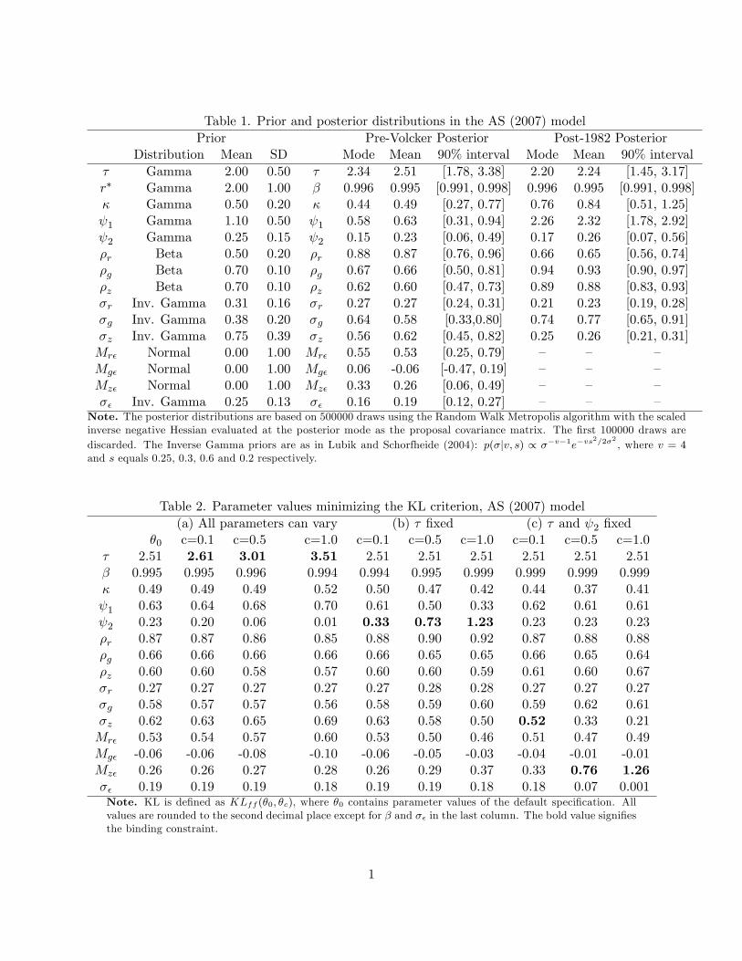
Table 1. Prior and posterior distributions in the AS (2007) modelPrior Pre-Volcker Posterior Post-1982 Posterior

Distribution Mean SD Mode Mean 90% interval Mode Mean 90% interval� Gamma 2.00 0.50 � 2.34 2.51 [1.78, 3.38] 2.20 2.24 [1.45, 3.17]r� Gamma 2.00 1.00 � 0.996 0.995 [0.991, 0.998] 0.996 0.995 [0.991, 0.998]� Gamma 0.50 0.20 � 0.44 0.49 [0.27, 0.77] 0.76 0.84 [0.51, 1.25] 1 Gamma 1.10 0.50 1 0.58 0.63 [0.31, 0.94] 2.26 2.32 [1.78, 2.92] 2 Gamma 0.25 0.15 2 0.15 0.23 [0.06, 0.49] 0.17 0.26 [0.07, 0.56]�r Beta 0.50 0.20 �r 0.88 0.87 [0.76, 0.96] 0.66 0.65 [0.56, 0.74]�g Beta 0.70 0.10 �g 0.67 0.66 [0.50, 0.81] 0.94 0.93 [0.90, 0.97]�z Beta 0.70 0.10 �z 0.62 0.60 [0.47, 0.73] 0.89 0.88 [0.83, 0.93]�r Inv. Gamma 0.31 0.16 �r 0.27 0.27 [0.24, 0.31] 0.21 0.23 [0.19, 0.28]�g Inv. Gamma 0.38 0.20 �g 0.64 0.58 [0.33,0.80] 0.74 0.77 [0.65, 0.91]�z Inv. Gamma 0.75 0.39 �z 0.56 0.62 [0.45, 0.82] 0.25 0.26 [0.21, 0.31]Mr� Normal 0.00 1.00 Mr� 0.55 0.53 [0.25, 0.79] � � �Mg� Normal 0.00 1.00 Mg� 0.06 -0.06 [-0.47, 0.19] � � �Mz� Normal 0.00 1.00 Mz� 0.33 0.26 [0.06, 0.49] � � �� Inv. Gamma 0.25 0.13 �� 0.16 0.19 [0.12, 0.27] � � �

Note. The posterior distributions are based on 500000 draws using the Random Walk Metropolis algorithm with the scaledinverse negative Hessian evaluated at the posterior mode as the proposal covariance matrix. The �rst 100000 draws arediscarded. The Inverse Gamma priors are as in Lubik and Schorfheide (2004): p(�jv; s) / ��v�1e�vs

2=2�2 , where v = 4and s equals 0.25, 0.3, 0.6 and 0.2 respectively.

Table 2. Parameter values minimizing the KL criterion, AS (2007) model(a) All parameters can vary (b) � �xed (c) � and 2 �xed

�0 c=0.1 c=0.5 c=1.0 c=0.1 c=0.5 c=1.0 c=0.1 c=0.5 c=1.0� 2.51 2.61 3.01 3.51 2.51 2.51 2.51 2.51 2.51 2.51� 0.995 0.995 0.996 0.994 0.994 0.995 0.999 0.999 0.999 0.999� 0.49 0.49 0.49 0.52 0.50 0.47 0.42 0.44 0.37 0.41 1 0.63 0.64 0.68 0.70 0.61 0.50 0.33 0.62 0.61 0.61 2 0.23 0.20 0.06 0.01 0.33 0.73 1.23 0.23 0.23 0.23�r 0.87 0.87 0.86 0.85 0.88 0.90 0.92 0.87 0.88 0.88�g 0.66 0.66 0.66 0.66 0.66 0.65 0.65 0.66 0.65 0.64�z 0.60 0.60 0.58 0.57 0.60 0.60 0.59 0.61 0.60 0.67�r 0.27 0.27 0.27 0.27 0.27 0.28 0.28 0.27 0.27 0.27�g 0.58 0.57 0.57 0.56 0.58 0.59 0.60 0.59 0.62 0.61�z 0.62 0.63 0.65 0.69 0.63 0.58 0.50 0.52 0.33 0.21Mr� 0.53 0.54 0.57 0.60 0.53 0.50 0.46 0.51 0.47 0.49Mg� -0.06 -0.06 -0.08 -0.10 -0.06 -0.05 -0.03 -0.04 -0.01 -0.01Mz� 0.26 0.26 0.27 0.28 0.26 0.29 0.37 0.33 0.76 1.26�� 0.19 0.19 0.19 0.18 0.19 0.19 0.18 0.18 0.07 0.001Note. KL is de�ned as KLff (�0; �c), where �0 contains parameter values of the default speci�cation. Allvalues are rounded to the second decimal place except for � and �� in the last column. The bold value signi�esthe binding constraint.

1

Table 3. KL and empirical distances between �c and �0, AS (2007) model(a) All parameters can vary (b) � �xed (c) � and 2 �xedc=0.1 c=0.5 c=1.0 c=0.1 c=0.5 c=1.0 c=0.1 c=0.5 c=1.0

KL 5.36E-07 1.57E-05 7.57E-05 1.04E-05 1.65E-04 3.35E-04 5.52E-05 4.24E-04 1.20E-3T=80 0.0509 0.0553 0.0621 0.0542 0.0679 0.0769 0.0608 0.0839 0.1147T=150 0.0513 0.0574 0.0672 0.0558 0.0761 0.0900 0.0651 0.0996 0.1492T=200 0.0515 0.0586 0.0703 0.0568 0.0811 0.0982 0.0677 0.1095 0.1719T=1000 0.0534 0.0710 0.1041 0.0665 0.1400 0.2007 0.0951 0.2339 0.4648Note. KL is de�ned as KLff (�0; �c) with �c given in the columns of Table 2. The empirical distance measureequals pff (�0; �c; 0:05; T ), where T is speci�ed in the last four rows of the Table.

Table 4. KL and empirical distances between monetary policy rules, AS (2007) model(a) Expected in�ation rule (b) Output growth rule

Indeterminacy Determinacy Indeterminacy DeterminacyKL 3.38E-14 4.24E-14 1.94E-05 6.00E-05T=80 0.0500 0.0500 0.0560 0.0614T=150 0.0500 0.0500 0.0583 0.0659T=200 0.0500 0.0500 0.0597 0.0686T=1000 0.0500 0.0500 0.0738 0.0976Note. Under indeterminacy, KL and the empirical distance measure are de�ned as KLfh(�0; �) andpfh(�0; �; 0:05; T ) with h and � being the spectral density and structural parameter vector of thealternative model and T speci�ed in the last four rows of the Table. Under determinacy, they arede�ned as KLfh(�D0 ; �

D) and pfh(�D0 ; �D; 0:05; T ).

Table 5. Parameter values minimizing the KL criterionIndeterminacy, LS (2004) model

(a) All parameters can vary (b) Mg� �xed�0 c=0.1 c=0.5 c=1.0 c=0.1 c=0.5 c=1.0

� 0.69 0.69 0.69 0.70 0.69 0.70 0.72� 0.997 0.998 0.999 0.999 0.953 0.999 0.999� 0.77 0.77 0.77 0.77 0.78 0.85 0.93 1 0.77 0.77 0.77 0.78 0.76 0.74 0.71 2 0.17 0.17 0.16 0.13 0.18 0.31 0.47�r 0.60 0.60 0.60 0.60 0.60 0.61 0.61�g 0.68 0.68 0.68 0.68 0.68 0.66 0.64�z 0.82 0.82 0.82 0.82 0.82 0.83 0.83�r 0.23 0.23 0.23 0.23 0.23 0.24 0.24�g 0.27 0.27 0.29 0.31 0.27 0.29 0.32�z 1.13 1.13 1.13 1.14 1.16 1.07 1.02�gz 0.14 0.15 0.11 0.07 0.13 0.17 0.20Mr� -0.68 -0.69 -0.64 -0.59 -0.66 -1.18 -1.68Mg� 1.74 1.84 1.24 0.74 1.74 1.74 1.74Mz� -0.69 -0.70 -0.65 -0.61 -0.66 -0.79 -0.89�� 0.20 0.13 0.39 0.50 0.10 0.16 0.01

Note. KL is de�ned as KLff (�0; �c). All values are rounded to the second decimalplace except for �. The bold value signi�es the binding constraint.

2

Table 6. KL and empirical distances between �c and �0Indeterminacy, LS (2004) model

(a) All parameters can vary (b) Mg� �xedc=0.1 c=0.5 c=1.0 c=0.1 c=0.5 c=1.0

KL 4.06E-07 1.22E-05 5.41E-05 5.45E-06 1.10E-03 3.90E-03T=80 0.0507 0.0550 0.0604 0.0520 0.1084 0.2021T=150 0.0510 0.0569 0.0646 0.0531 0.1392 0.2926T=200 0.0512 0.0580 0.0671 0.0538 0.1593 0.3518T=1000 0.0529 0.0686 0.0941 0.0604 0.4219 0.8739Note. KL is de�ned as KLff (�0; �c) with �c given in the columns of Table 5. Theempirical distance measure equals pff (�0; �c; 0:05; T ), where T is speci�ed in the lastfour rows of the Table.

Table 7. Parameter values minimizing the KL criterionDeterminacy, LS (2004) model

(a) All parameters can vary (b) 2 �xed�D0 c=0.1 c=0.5 c=1.0 c=0.1 c=0.5 c=1.0

� 0.54 0.54 0.55 0.55 0.55 0.56 0.57� 0.992 0.900 0.900 0.900 0.900 0.900 0.900� 0.58 0.62 0.62 0.62 0.63 0.65 0.67 1 2.19 2.09 1.71 1.23 2.29 2.69 3.19 2 0.30 0.40 0.80 1.30 0.30 0.30 0.30�r 0.84 0.84 0.84 0.84 0.84 0.86 0.88�g 0.83 0.83 0.83 0.83 0.83 0.84 0.84�z 0.85 0.85 0.85 0.85 0.85 0.85 0.85�r 0.18 0.18 0.18 0.18 0.18 0.18 0.19�g 0.18 0.18 0.18 0.18 0.18 0.19 0.19�z 0.64 0.64 0.64 0.64 0.64 0.64 0.64�gz 0.36 0.36 0.36 0.36 0.35 0.32 0.29

Note. KL is de�ned as KLff (�D0 ; �Dc ). All values are rounded to the second decimalplace except for �. The bold value signi�es the binding constraint.

Table 8. KL and empirical distances between �Dc and �D0 ,

Determinacy, LS (2004) model(a) All parameters can vary (b) 2 �xedc=0.1 c=0.5 c=1.0 c=0.1 c=0.5 c=1.0

KL 1.06E-07 1.28E-05 6.26E-05 1.05E-04 2.10E-03 6.20E-03T=80 0.0504 0.0544 0.0602 0.0650 0.1479 0.2729T=150 0.0506 0.0563 0.0648 0.0713 0.2017 0.4011T=200 0.0507 0.0573 0.0675 0.0751 0.2373 0.4810T=1000 0.0515 0.0683 0.0970 0.1178 0.6541 0.9659Note. KL is de�ned as KLff (�D0 ; �Dc ) with �Dc given in the columns of Table 7. Theempirical distance measure equals pff (�D0 ; �

Dc ; 0:05; T ), where T is speci�ed in the last

four rows of the Table.

3

Table 9. Empirical distances by altering the Taylor rule parameters, LS(2004) model 1 2 �r �r

�Dj � �D0 KL T = 80 T = 1000

�D0 2.1900 0.3000 0.8400 0.1800 � � � �(a) Direction 1

�D1 2.1194 0.3720 0.8399 0.1800 0.1009 1.23E-06 0.0516 0.0555�D2 2.0486 0.4442 0.8398 0.1800 0.2019 5.17E-06 0.0533 0.0617�D3 1.9779 0.5163 0.8397 0.1801 0.3029 1.22E-05 0.0552 0.0688�D4 1.9072 0.5884 0.8396 0.1801 0.4039 2.28E-05 0.0572 0.0769�D5 1.8365 0.6605 0.8395 0.1801 0.5049 3.75E-05 0.0593 0.0863�D6 1.7658 0.7326 0.8394 0.1802 0.6059 5.70E-05 0.0617 0.0969�D7 1.6951 0.8048 0.8392 0.1802 0.7069 8.19E-05 0.0642 0.1092�D8 1.6244 0.8769 0.8391 0.1803 0.8079 1.13E-04 0.0670 0.1233�D9 1.5537 0.9490 0.8390 0.1803 0.9089 1.52E-04 0.0700 0.1395�D10 1.4830 1.0212 0.8389 0.1804 1.0099 1.98E-04 0.0733 0.1583

(b) Direction 2�D1 2.2193 0.2701 0.8400 0.1800 0.0419 1.99E-07 0.0505 0.0520�D2 2.2487 0.2401 0.8401 0.1800 0.0839 7.83E-07 0.0511 0.0541�D3 2.2781 0.2101 0.8401 0.1800 0.1259 1.73E-06 0.0516 0.0562�D4 2.3075 0.1801 0.8402 0.1800 0.1679 3.02E-06 0.0521 0.0583�D5 2.3369 0.1501 0.8402 0.1800 0.2099 4.64E-06 0.0526 0.0604�D6 2.3664 0.1201 0.8403 0.1800 0.2519 6.56E-06 0.0531 0.0626�D7 2.3958 0.0901 0.8403 0.1800 0.2939 8.77E-06 0.0536 0.0648�D8 2.4252 0.0601 0.8404 0.1800 0.3359 1.12E-05 0.0541 0.0670�D9 2.4546 0.0302 0.8404 0.1799 0.3779 1.40E-05 0.0546 0.0692�D10 2.4840 0.0002 0.8405 0.1799 0.4199 1.70E-05 0.0551 0.0714Note. �Dj represent equally spaced points taken from the curve determined by the smallest eigenvaluefrom changing the four parameters in the monetary policy rule. The curve is extended from �D0 alongtwo directions. Along Direction 1, the curve is truncated when k�Dj � �D0 k exceeds 1. Along Direction2, the curve is truncated at the closest point to zero where 2 is still positive. KL is de�ned asKLff (�

D0 ; �

Dj ). The last two columns are empirical distance measures de�ned as pff (�

D0 ; �

Dj ; 0:05; T ).

4

Table 10. Structural parameters in the SW (2007) model�ga Cross-corr.: tech. and exog. spending shocks�w Wage mark-up shock MA�p Price mark-up shock MA� Share of capital in production Elasticity of capital utilization adjustment cost' Investment adjustment cost�c Elasticity of intertemporal substitution� Habit persistence�p Fixed costs in production�w Wage indexation�w Wage stickiness�p Price indexation�p Price stickiness�l Labor supply elasticityr� Taylor rule: in�ation weightr�y Taylor rule: feedback from output gap changery Taylor rule: output gap weight� Taylor rule: interest rate smoothing�a Productivity shock AR�b Risk premium shock AR�g Exogenous spending shock AR�i Interest rate shock AR�r Monetary policy shock AR�p Price mark-up shock AR�w Wage mark-up shock AR�a Productivity shock std. dev.�b Risk premium shock std. dev.�g Exogenous spending shock std. dev.�i Interest rate shock std. dev.�r Monetary policy shock std. dev.�p Price mark-up shock std. dev.�w Wage mark-up shock std. dev. Trend growth rate: real GDP, In�., Wages

100(��1�1) Discount rate

5

Table 11. Parameter values miminizing the KL criterion, SW(2007) model(a) All parameters can vary (b) ' �xed

�D0 c=0.1 c=0.5 c=1.0 c=0.1 c=0.5 c=1.0�ga 0.52 0.52 0.52 0.52 0.52 0.52 0.52�w 0.84 0.84 0.84 0.84 0.84 0.83 0.82�p 0.69 0.69 0.69 0.69 0.69 0.70 0.71� 0.19 0.19 0.19 0.19 0.19 0.19 0.20 0.54 0.54 0.54 0.53 0.54 0.56 0.59' 5.74 5.84 6.24 6.74 5.74 5.74 5.74�c 1.38 1.38 1.38 1.38 1.37 1.42 1.48� 0.71 0.71 0.72 0.72 0.71 0.69 0.67�p 1.60 1.60 1.61 1.61 1.60 1.61 1.63�w 0.58 0.58 0.58 0.57 0.58 0.58 0.57�w 0.70 0.70 0.70 0.71 0.71 0.67 0.64�p 0.24 0.24 0.24 0.24 0.24 0.24 0.25�p 0.66 0.66 0.66 0.66 0.66 0.66 0.66�l 1.83 1.83 1.85 1.86 1.93 1.33 0.83r� 2.04 2.04 2.02 2.01 2.04 2.06 2.08r�y 0.22 0.22 0.22 0.22 0.22 0.23 0.25ry 0.08 0.08 0.08 0.08 0.08 0.08 0.08� 0.81 0.81 0.81 0.81 0.81 0.81 0.81�a 0.95 0.95 0.95 0.95 0.95 0.95 0.95�b 0.22 0.22 0.22 0.22 0.22 0.23 0.24�g 0.97 0.97 0.97 0.97 0.97 0.97 0.97�i 0.71 0.71 0.70 0.70 0.71 0.71 0.72�r 0.15 0.15 0.15 0.15 0.15 0.16 0.17�p 0.89 0.89 0.89 0.89 0.89 0.89 0.90�w 0.96 0.96 0.96 0.96 0.96 0.96 0.96�a 0.45 0.45 0.45 0.45 0.45 0.45 0.44�b 0.23 0.23 0.23 0.23 0.23 0.23 0.22�g 0.53 0.53 0.53 0.53 0.53 0.53 0.53�i 0.45 0.45 0.45 0.45 0.45 0.45 0.45�r 0.24 0.24 0.24 0.24 0.24 0.24 0.25�p 0.14 0.14 0.14 0.14 0.14 0.14 0.14�w 0.24 0.24 0.24 0.24 0.24 0.24 0.24 0.43 0.43 0.43 0.42 0.45 0.34 0.24

100(��1 � 1) 0.16 0.17 0.19 0.22 0.15 0.22 0.29Note. KL is de�ned as KLff (�D0 ; �Dc ). All values are rounded to the second decimal place. The bold valuesigni�es the binding constraint.

6

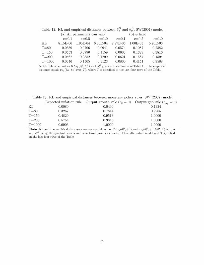
Table 12. KL and empirical distances between �Dc and �D0 , SW(2007) model

(a) All parameters can vary (b) ' �xedc=0.1 c=0.5 c=1.0 c=0.1 c=0.5 c=1.0

KL 8.15E-06 1.86E-04 6.66E-04 2.87E-05 1.00E-03 5.70E-03T=80 0.0539 0.0706 0.0941 0.0574 0.1087 0.2582T=150 0.0553 0.0796 0.1159 0.0603 0.1389 0.3816T=200 0.0562 0.0852 0.1299 0.0621 0.1587 0.4594T=1000 0.0646 0.1505 0.3123 0.0800 0.4151 0.9588

Note. KL is de�ned as KLff (�D0 ; �Dc ) with �Dc given in the columns of Table 11. The empiricaldistance equals pff (�D0 ; �

Dc ; 0:05; T ), where T is speci�ed in the last four rows of the Table.

Table 13. KL and empirical distances between monetary policy rules, SW (2007) modelExpected in�ation rule Output growth rule (ry = 0) Output gap rule (r�y = 0)

KL 0.0080 0.0499 0.1334T=80 0.3267 0.7844 0.9965T=150 0.4829 0.9513 1.0000T=200 0.5754 0.9845 1.0000T=1000 0.9903 1.0000 1.0000Note. KL and the empirical distance measure are de�ned as KLfh(�D0 ; �D) and pfh(�D0 ; �D; 0:05; T ) with hand �D being the spectral density and structural parameter vector of the alternative model and T speci�edin the last four rows of the Table.

7

Table 14. Empirical distances by altering the Taylor rule parameters, SW(2007) modelr� r�y ry � �r

�Dj � �D0 KL T=80 T=150�D0 2.0400 0.2200 0.080 0.8100 0.2400 � � � �

a) Direction 1�D1 2.0296 0.2233 0.0794 0.8065 0.2511 0.0160 0.0019 0.1644 0.2175�D2 2.0197 0.2267 0.0789 0.8029 0.2627 0.0320 0.0072 0.3562 0.5023�D3 2.0103 0.2302 0.0784 0.7993 0.2746 0.0480 0.0156 0.5723 0.7635�D4 2.0015 0.2338 0.0779 0.7956 0.2869 0.0639 0.0266 0.7513 0.9131�D5 1.9931 0.2375 0.0774 0.7919 0.2995 0.0799 0.0398 0.8699 0.9737�D6 1.9851 0.2412 0.0770 0.7882 0.3123 0.0958 0.0549 0.9368 0.9930�D7 1.9775 0.2450 0.0766 0.7845 0.3253 0.1117 0.0716 0.9707 0.9983�D8 1.9703 0.2488 0.0762 0.7807 0.3386 0.1276 0.0894 0.9867 0.9996�D9 1.9634 0.2527 0.0758 0.7769 0.3519 0.1435 0.1082 0.9940 0.9999�D10 1.9568 0.2565 0.0755 0.7731 0.3655 0.1593 0.1278 0.9973 1.0000

b) Direction 2�D1 2.0482 0.2176 0.0805 0.8126 0.2320 0.0120 0.0011 0.0925 0.1217�D2 2.0567 0.2153 0.0809 0.8152 0.2243 0.0240 0.0045 0.1620 0.2552�D3 2.0655 0.2131 0.0814 0.8177 0.2169 0.0360 0.0103 0.2654 0.4523�D4 2.0746 0.2109 0.0819 0.8202 0.2098 0.0480 0.0186 0.4018 0.6724�D5 2.0840 0.2089 0.0825 0.8226 0.2031 0.0599 0.0293 0.5583 0.8506�D6 2.0937 0.2069 0.0830 0.8249 0.1968 0.0718 0.0424 0.7115 0.9510�D7 2.1037 0.2050 0.0836 0.8272 0.1908 0.0837 0.0579 0.8370 0.9890�D8 2.1139 0.2033 0.0842 0.8295 0.1852 0.0956 0.0755 0.9219 0.9984�D9 2.1243 0.2016 0.0848 0.8317 0.1800 0.1075 0.0952 0.9688 0.9998�D10 2.1349 0.2000 0.0854 0.8338 0.1751 0.1193 0.1167 0.9897 1.0000Note. �Dj represent equally spaced points taken from the curve determined by the smallest eigenvaluefrom changing the �ve parameters in the monetary policy rule. The curve is extended from �D0 in twodirections until the empirical distance reaches 1 with T=150 or the parameter boundaries are reached.KL is de�ned as KLff (�D0 ; �

Dj ). The last two columns are empirical distance measures de�ned as

pff (�D0 ; �

Dj ; 0:05; T ).

8

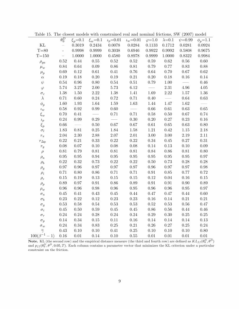
Table 15. The closest models with constrained real and nominal frictions, SW (2007) model�D0 �p=0:1 �w=0:1 �p=0:01 �w=0:01 '=1:0 �=0:1 =0:99 �p=1:1

KL � 0.3019 0.2434 0.0078 0.0284 0.1133 0.1712 0.0281 0.0924T=80 - 0.9998 0.9999 0.3038 0.6946 0.9922 0.9992 0.5808 0.9675T=150 � 1.0000 1.0000 0.4580 0.8978 0.9999 1.0000 0.8322 0.9984�ga 0.52 0.44 0.55 0.52 0.52 0.59 0.62 0.56 0.60�w 0.84 0.64 0.09 0.86 0.81 0.79 0.77 0.83 0.88�p 0.69 0.12 0.61 0.41 0.76 0.64 0.70 0.67 0.62� 0.19 0.18 0.20 0.19 0.21 0.20 0.18 0.16 0.14 0.54 0.96 0.80 0.54 0.51 0.79 1.00 � � 0.46' 5.74 3.27 2.00 5.73 6.12 � � 2.31 4.96 4.05�c 1.38 1.50 2.22 1.38 1.41 1.69 2.22 1.57 1.36� 0.71 0.60 0.24 0.72 0.71 0.40 � � 0.64 0.63�p 1.60 1.93 1.64 1.59 1.63 1.44 1.47 1.62 � ��w 0.58 0.92 0.99 0.60 � � 0.66 0.61 0.63 0.65�w 0.70 0.41 � � 0.71 0.71 0.58 0.50 0.67 0.74�p 0.24 0.99 0.29 � � 0.30 0.20 0.27 0.23 0.16�p 0.66 � � 0.50 0.67 0.67 0.61 0.65 0.63 0.80�l 1.83 0.81 0.25 1.84 1.58 1.21 0.42 1.15 2.18r� 2.04 2.30 2.88 2.07 2.01 3.00 3.00 2.19 2.11r�y 0.22 0.21 0.33 0.22 0.22 0.34 0.45 0.27 0.31ry 0.08 0.07 0.10 0.08 0.08 0.14 0.13 0.10 0.09� 0.81 0.79 0.81 0.81 0.81 0.84 0.86 0.81 0.80�a 0.95 0.95 0.94 0.95 0.95 0.95 0.95 0.95 0.97�b 0.22 0.32 0.73 0.22 0.22 0.50 0.73 0.28 0.28�g 0.97 0.96 0.97 0.97 0.97 0.96 0.97 0.97 0.98�i 0.71 0.80 0.86 0.71 0.71 0.91 0.85 0.77 0.72�r 0.15 0.19 0.13 0.15 0.15 0.12 0.04 0.16 0.15�p 0.89 0.97 0.91 0.86 0.89 0.91 0.91 0.90 0.89�w 0.96 0.96 0.98 0.96 0.95 0.96 0.96 0.95 0.97�a 0.45 0.41 0.43 0.45 0.44 0.47 0.47 0.44 0.60�b 0.23 0.22 0.12 0.23 0.23 0.16 0.14 0.21 0.21�g 0.53 0.58 0.54 0.53 0.53 0.52 0.53 0.56 0.47�i 0.45 0.50 0.59 0.45 0.45 0.86 0.56 0.44 0.46�r 0.24 0.24 0.28 0.24 0.24 0.29 0.30 0.25 0.25�p 0.14 0.34 0.15 0.11 0.16 0.14 0.14 0.14 0.13�w 0.24 0.34 0.83 0.25 0.21 0.26 0.27 0.25 0.24 0.43 0.10 0.10 0.41 0.25 0.10 0.10 0.10 0.80

100(��1 � 1) 0.16 0.01 0.14 0.10 0.55 0.01 0.01 0.01 0.01Note. KL (the second row) and the empirical distance measure (the third and fourth row) are de�ned as KLff (�D0 ; �D)and pff (�D0 ; �

D; 0:05; T ). Each column contains a parameter vector that minimizes the KL criterion under a particularconstraint on the friction.

9

Documents

Local and Global Parameter Identi–cation in DSGE … · Local and Global Parameter Identi–cation in DSGE Models Allowing for Indeterminacy ... December 19, 2012; this version: