Local energy system -Comparing direct current (LVDC) and

Ind

ust

rial E

lectr

ical En

gin

eerin

g a

nd

A

uto

matio

n

CODEN:LUTEDX/(TEIE-5450)/1-56(2020)

Local energy system- Comparing direct current (LVDC) and

alternating current (LVAC)

Markus Alm

Division of Industrial Electrical Engineering and Automation Faculty of Engineering, Lund University

Table of Contents Abstract 3

Popular Science Summary 4

Foreword 6

Abbreviations 7

1. Introduction 8

1.1. Background 8

1.1.1. Previous Projects involving LVDC 11

1.2. Purpose 13

1.3. Project details 14

1.3.1. Case study 14

1.3.2. Challenges 14

1.3.3. Limitation 15

2. Theory 16

2.1. The difference between LVAC and LVDC 16

2.2. Components 17

2.2.1. Transformer 17

2.2.2. AC/DC rectifier 18

2.2.3. DC/AC inverter 18

2.2.4. DC/DC converter 19

2.2.5. Cables 20

2.3. Solar power 21

2.4. Batteries (ESS) 22

2.5. Separated and interconnected distribution LES 25

2.6. Standards and Praxis 26

2.7. Risks with LVDC 27

3. Method 28

3.1. Dimensioning 28

3.2. In data 29

3.2.1. PV production 29

3.2.2. Load data 29

3.3. Scenarios and Models 30

3.3.1. LVAC 31

1

3.3.1.1. Scenario Case #1 - Separated 33

3.3.1.2. Scenario Case #2 - Interconnected 33

3.3.2. LVAC with ESS 33



3.3.3. LVDC 34



3.3.4. LVDC with ESS 37



3.4. Comparison 38

4. Results 39

4.1. Scenario Case #1 and Case #5 39




4.5. Efficiency and load demand from the AC grid 42

4.6. Self-sufficiency 43

4.7. Energy storage 45

5. Analysis 47

5.1. Result of battery simulation 47

5.2. Overproduction 47

5.3. LVAC vs. LVDC 48

5.4. Separated vs. Interconnected 49

5.5. Battery interconnection 49

5.6. Standards and voltage level 49

5.7. Losses 50

6. Conclusion & Future Work 51

6.1. Conclusion 51

6.2. Future Work 52

References 54

2

Abstract Local energy system - comparing direct current (LVDC) and alternating current (LVAC) This thesis uses a case study to compare the viability of using direct current instead of alternating current to supply power to 5 buildings in a local energy system (LES). The case study sought to show how using LVDC instead of LVAC could increase the effectiveness of solar panels (PV), batteries and interconnecting buildings into a local energy system (LES). The system studied in this thesis was designed so the buildings would share the same carrier as the LES, so the LVDC LES would have DC-based buildings.

The case study found that adding batteries to an LVDC system would increase self-sufficiency less than adding them to an LVAC system, and that the LVAC system would require more power from an external grid. The case study also found that using an LVDC system increased the system's overproduction and self-sufficiency for all LVDC cases.

The thesis concluded that building an LVDC system where buildings could share solar overproduction and battery power, reduced the amount of power needed from an external grid by 3,5% compared to an LVAC system with separate buildings and no batteries. The LVDC system was also 23% more self-sufficient than its LVAC counterpart.

3

Popular Science Summary Due to the ongoing climate changes, there is a global interest in removing society’s dependence on fossil fuels. In Sweden there is a goal to have net zero carbon emissions by 2040. For a private energy consumer this means using more renewable energy to supply electric power and heat to their homes and using electric powered vehicles, instead of gas- or diesel-powered cars etc. In order to accomplish this, many different solutions are being proposed. One interesting proposed solution is to make the consumer become an energy producer by installing solar panels in their homes and buildings. Energy and construction companies have started to investigate and invest in local energy systems (LES) to help utilize the produced solar power within and between buildings, in order to maximize the efficiency of these solar panels and make them a more viable competitor in the energy market.

These LES’s create an interesting opportunity, since the buildings share their produced energy between themselves instead of sending it directly to the external AC grid. Since the LES isn’t directly connected to the AC grid, it would also be possible to run the LES as DC instead of the standard AC. Using DC in the LES would increase the efficiency since more and more of our daily energy usage and production is DC based, such as battery powered devices, heating and charging electric vehicles. DC devices being used today include adaptors to convert the AC voltage from a wall socket into DC voltage for the device, which causes unnecessary power losses.

These LES’s will become more and more common in the coming years, as new residential areas are built with solar power generation in mind. Hence, it is interesting and important to see which type of LES would be best at using solar power. There are three main differentiating factors to look at, one is interconnecting buildings together locally so they can share their solar production between each other. Another area is the batteries, which are used to store excess solar production within the LES and finally, to use low voltage DC (LVDC) instead of low voltage AC (LVAC) to improve the overall efficiency of the LES.

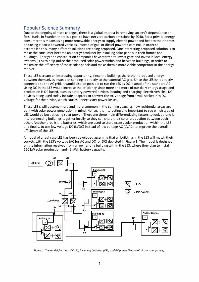
A model of a real case LES has been developed assuming that all buildings in the LES will match their sockets with the LES’s voltage (AC for AC and DC for DC) depicted in Figure 1. The model is designed on the information received from an owner of a building within the LES, where they plan to install 160 kW solar production and 45 kWh battery capacity.

Figure 1: The model for the LVDC LES, including batteries (ESS) and PV panels (Photovoltaic, or solar panels).

4

The model input data is based on the energy consumption characteristics and solar production for one year. The model includes losses from converters and wires to give an accurate simulation of the power flow in an actual LES. The simulations showed that the LES had a 25% increase in self-sufficiency when switching from LVAC to LVDC and lowered the power demand from the larger AC grid by 1,6%. The self-sufficiency is how much of the LES load demand is covered by self produced solar electricity.

A best-case scenario for solar power usage was created by interconnecting the buildings and adding batteries to an LVDC system. When comparing the results from this case to an LVAC case, where none of these changes were made, showed the following improvements:

● As stated previously the switch from AC to DC increased efficiency by 1,6%.

● The self-sufficiency increased from 8,3% to 11,3%.

● The total yearly power demand from the AC grid was reduced by 3,5%.

● This case also fully charged all its batteries 242 hours per year, using only solar power.

From these results it was concluded that, from a technical perspective and in case of overproduction, using an interconnected LES is preferable compared to letting buildings sell their solar production to an external grid. The results showed an overall increase in efficiency and self-sufficiency when the LES ran on LVDC instead of LVAC and the LVDC LES makes better use of batteries than the LVAC LES. The interconnection of buildings in a LES and the addition of batteries both provided increased self-sufficiency. Hence, from a technical perspective, interconnecting buildings and using batteries is a recommended approach when designing a LES.

The results made it apparent that the solar energy production capacity and battery sizes that were specified for this case study were too conservatively chosen. Therefore, from a technical perspective, it is recommended to increase the solar power-and battery capacity to make the system more capable of covering the LES’s loads and thereby achieve higher self-sufficiency.

5

Foreword The thesis will serve as the final part of the master of science and engineering, electrical engineering program at Lunds University. The thesis was written by Markus Alm from november 2018 to december 2019. The majority of the thesis work was conducted at E.ON Energidistribution AB in Malmö. The thesis was made to test the technical viability of an LVDC LES against an LVAC LES.

I would like to thank Peder Kjellén for being my supervisor and helping me with writing the report and guiding me through working on this thesis. He helped me come to terms with how to limit and later conclude this thesis. I want to thank my other supervisor Jörgen Svensson at IEA LTH, Lund University. For helping in finishing this report and working out the purpose and goal of this thesis, it wouldn’t have been finished if not for his contributions. Further, I want to thank Daniel Salomonsson at E.ON for helping in the first half of this thesis. His contribution includes the idea to have the buildings in the LVDC LES be DC-based, which strengthened the results of the LVDC simulations and made them easier to create. I also want to thank Sebastian Jansson for obtaining the data for the EV garage for me.

Finally, I want to give special thanks to Ingmar Leisse at E.ON for coming into the thesis work later during the simulations and guiding me through how to complete them. Without his help, this thesis would not have been completed. As he is the one who figured out that the simulation program used before PyPSA wouldn’t have worked for what we were planning and helped me build and check every case model in PyPSA. I also want to thank him for obtaining the load and solar production data that all simulations are based on, twice.

- Markus Alm, Lund, October 2019

6

Abbreviations AC - Alternating Current

DC - Direct Current

LVAC - Low Voltage Alternating Current

LVDC - Low Voltage Direct Current

HVAC - High Voltage Alternating Current

HVDC - High Voltage Direct Current

LES - Local Energy System

PV - Photovoltaic

EV - Electric Vehicle

ESS - Energy Storage System

SoC - State of Charge

SoF - State of Function

SoH - State of Health

DoD - Depth of Discharge

RES - Renewable Energy Source

7

1. Introduction This chapter seeks to familiarize the reader with the background of Low Voltage Direct Current (LVDC) local energy systems (LES) and the interest in using them. Then, previous projects involving LVDC will be presented to provide a foundation for the thesis theory and conclusion. Afterwards, this thesis purpose will be stated and a description of the thesis project will be given . Next is a subsection on the challenges with building an LVDC LES. Finally, the chapter is ended by detailing the limitations of the thesis in its own subsection.

1.1. Background Electricity is an integral part of modern society, and with an expanding need for more power the size of the electrical system is constantly increasing. The power supply for all facets of society has been based on alternating current (AC), specifically Low Voltage Alternating Current (LVAC), ever since its creation in the late 19th century. Considering these two statements present an opportunity to improve upon previous technology that has been used in these systems for decades. This leads to studying the potential of using direct current (DC) or more specifically, LVDC as the electricity carrier for local distribution. To understand how we have found ourselves in these circumstances and why there is an interest in DC, the history of DC will be explained briefly below.

The history of alternating current and direct current as energy distribution mediums

In 1888 Thomas Edison competed against George Westinghouse and Nikola Tesla to decide the future standard for current in the United States. The Edison Lamp Company, which would merge in 1889 to become the Edison General Electric company, used DC and the Westinghouse Electric Corporation used AC. This event was dubbed the “war of the currents” and was won by the Westinghouse corporation, because of ACs ability to change its voltage with transformers. The transformer could convert AC to a higher voltage, so it could be transported long distances with low losses, something that couldn’t be accomplished with DC at the time. Hence, in a DC system the power source had to be located in the cities and in an AC system it could be located outside the cities. In 1893 the two corporations both sought the right to power the Chicago World Fair, which the Westinghouse Electric Corporation won, due to providing power for a $155000 lower price than the Edison General Electric company (Lantero, 2014). In the same year the Westinghouse Corporation managed to power the city of Buffalo, New York with hydropower electricity from the Niagara Falls, located 26 miles away from the city (Nix, 2015). This would be the end of the “war of the currents” and AC was adopted as the distribution standard for over 100 years.

However, DC wasn’t completely abandoned, as it became the chosen distribution standard for the telecom industry. DC was selected because it didn’t cause any audio disturbances (noise), since it doesn’t possess a frequency unlike AC. When telecommunication was established it used ripples in the DC current to transmit the audio from the source to the receiver. If AC had been used instead there would be an audible hum in the receiver, due to the ACs base frequency. Later, it became possible to remove the AC audio disturbance using frequency filters. However, by that point DC could be transmitted over long distances and therefore AC did not replace DC in the telecom industry as it would be unnecessary. Aside from telecom DC is currently being used as High Voltage Direct Current (HVDC) in long distance power transmission.

HVDC as a technology has existed since the early 1880’s, but did not see any commercial use until the 1950’s. This was due to the difficulty of converting high voltage AC to high voltage DC. In 1929 the mercury arc valve was patented by Uno Lamm and he used it to construct the first commercial HVDC system, connecting the Swedish mainland to Gotland in 1954. The mercury arc valve is a rectifier that can convert high voltage AC to DC. However, the mercury arc valve had a significant problem, as

8

mercury poses an environmental risk. In the 1970’s the thyristor rectifier became available for use in commercial HVDC and eliminated the HVDC conversion problem. The new converter completely replaced the mercury arc valve, since it was more cost effective and had a low environmental risk. Eventually, the thyristor rectifier was in turn also replaced by the IGBT AC/DC converter that is used today (Peake, 2010). HVDC has since then been used to transfer large amounts of power over long distances, where it can achieve a higher efficiency than High Voltage Alternating Current (HVAC). Both HVDC and telecommunication systems show the potential of DC power and they can aid in how to implement LVDC distribution, which has garnered increased interest due to an increasing demand for renewable energy.

The current state of power generation and LVDC

Renewable energy is becoming more relevant to the goal of modern energy production due to the documented and increasingly relevant consequences of using fossil power and the changes to the climate that it’s causing. In 2013 IEA(IEA, 2013) estimated that residential housing caused approximately 17% of all CO2 emissions of final direct-energy consumers. To reduce CO2 emissions, effort is being put into renewable energy sources such as wind-and solar power. In Sweden there is an effort to install solar panels to help alleviate the environmental impact caused by residential buildings. The total capacity of solar power production at the end of 2018 was 231 MW, a 65% increase from the total 140 MW that was installed before 2017 (Berard, 2018). This is a growing part of the Swedish energy mix, comprising about 0,14% of the total electricity production (SCB, 2018). Wind power is the most prevalent renewable energy source being used to replace fossil fuels and at the end of 2017 wind power comprised 9% of the total energy mix. The goal to achieve a fully renewable energy mix in 2040, would require up to 60 TWh of wind power (Palmblad, 2018). The amount of wind power required for a fully renewable energy mix will depend on the efficiency and usage of other renewable sources like solar power. As solar power is easier to integrate into neighborhoods and cities, there is an effort put forth to increase its viability and to fulfill the 2040 goal.

Figure 1: The installed power of PV in Sweden, yellow is for 2016 and blue is for 2017 (Berard, 2018)-(Edited).

It has been determined by several research projects and thesis such as (Flyckt, 2018) and (Stierna, 2018) that using an LVDC LES will contribute to increased profitability of solar systems, as the LES can eliminate conversion steps and gives the ability to efficiently share solar production between

9

buildings. An LVDC LES would also allow DC loads to be powered through a wall socket without the need for AC/DC conversion. DC loads today include lighting, electronics, electric vehicle (EV) charging and possibly also heating. Using LVDC would allow these DC loads to remove internal transformers and rectifiers, thus increasing the efficiency of these loads (Lotfi & Khodaei, 2015). Since these DC loads are used frequently in residential buildings, it has been estimated that up to 50% of residential power consumption is done via DC loads (Rodriguez-Diaz et al, 2015). Because of an increasing demand for solar power and the increasing amount of DC loads there is an interest in developing LVDC systems around the world. Many research papers and demonstration projects involving LVDC have been developed so far and the number is growing. These tend to be in the form of microgrids, a relatively new form of LES, which will be explained below.

A microgrid is a LES, a small distribution grid connecting a few buildings, containing some sort of energy storage system (ESS). This gives the distribution grid the ability to disconnect itself from the larger grid and function as an isolated network (island). Microgrids also include some renewable energy sources (RES), such as wind and solar power. While an LVDC LES is being implemented, the idea of turning it into a microgrid is often considered as this is easier than trying to convert an entire AC grid to DC. The goal of LVDC projects usually involves increasing LES efficiency and improving the self-sufficiency of the microgrid. Self-sufficiency is key to increase the profitability of RES and microgrids, since their value lies in reducing the reliance on a larger grid. Increasing the amount of microgrids and renewable energy will cause decentralisation of power sources and create increasing imbalance in a larger grid, which will need to be compensated in some way.

The development of renewables and closing of nuclear power plants is starting a decentralization of power production. The decentralization causes more difficult power balancing, as it consists of many small power production facilities. Renewables are also dependent on weather and function differently from each other depending on the weather; Wind power can function fully with heavy cloud cover that reduces solar production. Decentralization will make it easier to create microgrids, but it will make it more difficult to balance the power throughout a larger grid. Therefore, a change to consumer patterns could be needed to account for the more difficult power balancing.

E.ON wants to study the benefits of using an LVDC LES instead of an LVAC LES for future reference as they have an interest in building microgrids. This comes as a natural addition to their expansion in renewable energy. E.ONs clients have an interest in installing LES or microgrids for their future building projects since it can reduce the amount of money they have to spend on buying electricity from an external grid. The following section will present some demonstration sites and explain what has been learnt from them.

10

1.1.1. Previous Projects involving LVDC To establish a basis for what is to be expected from this theoretical project and provide something to compare its results to, several real LVDC projects are described below. These projects focus on different aspects of this thesis and together form an overall goal to try and reach with this thesis. The projects included guidelines for the efficiency increase when switching from AC to DC, increased self sufficiency provided by batteries and how connecting buildings together can improve their own-usage of locally generated solar power. The Xiamen University project is included as it provided a surprising result about what can be powered using solar panels on a building, which is useful for discussion about this thesis result.

Vasakronan together with Ferroamp has built an LVDC distribution grid connecting 4 buildings in Uppsala science park. This distribution grid was studied and simulated in the thesis paper (Flyckt, 2018). The four buildings in the science park share 236,4 kWp of solar power and import the remainder of the electricity demand from the nearby AC grid. The buildings in the system are AC based with a rectifier to the distribution grid. Simulating an LVDC distribution grid revealed an average increase in power usage of the residential electricity during October-April for all buildings, compared to an LVAC distribution grid. A power peak analysis determined that the distribution grid imported more power after 15:00 CET during daily operation.

Figure 2: Aerial photo of the area in Uppsala science park with the LVDC distribution grid coloured in yellow (Flyckt, 2018).

The own usage of PV production was at 99,2% in the LVDC distribution grid and 81,6% in the LVAC distribution grid. The result of the simulations was that switching to an LVDC distribution grid caused a power savings of 34MWh of energy per year. Using the replacement value method, the economic analysis found that the savings results in a 178k SEK cost reduction over the calculation period. The power peak analysis showed that installing solar panels moves the daily power peaks to 2 hours later in the afternoon, so the solar power production only covers 2 hours of the high consumption period. Hence, the conclusion drawn is that there is a mismatch between solar production and power consumption. Therefore, Vasakronan has shown an interest in connecting ESS to the LVDC system. The thesis concluded that installing a 6 kW battery would be unprofitable, as it only resulted in an annual saving of 2880 SEK for a total investment cost of 63k SEK.

Xiamen University has built a DC microgrid at the engineering building of the College of Energy at Xiang’an Campus. The microgrid is the subject of the study (Fengyan et al, 2015), where the feasibility of implementing DC microgrids for commercial buildings is investigated. According to (Fengyan et al, 2015), the purpose of Xiamen University’s LVDC microgrid is to power the building’s

11

DC loads with PV production and to power the AC loads from the AC grid. The building's main power supply is 150 kWp of solar panels, located on top of the university’s engineering building.

Figure 3: The School of Energy with PV panels at Xiang’an Campus (Fengyuan et al, 2015).

The DC microgrid is run on a bus voltage of 380 V and supplies power to 30 kW air conditioning, 40 kW EV-charging and 20 kW LED lighting. To retain a stable 380 V (±5%) in the system, it requires a 67 kWh lead acid battery and a 160 kW AC/DC backup unit. (Fengyan et al, 2018) found that if the 150kW of solar panels were to power only LED lighting, the solar microgrid system could power a 16-story office building with the same roof area. The study concluded that using solar panels on high rise office buildings could lead to large energy savings, reduced CO2 emissions and ability to reduce the peak load without taking up extra ground area. Further, the study found that both air conditioning and EV-charging required more power than the solar installation can supply.

A Working Lab (AWL) is a development project by Chalmers in Johanneberg Science Park that was completed in the summer of 2019 (Akademiska Hus, 2018)(Chalmers, 2017). One of several goals with the development project was to supply certain parts of the Working Lab with lighting and ventilation through an internal DC LES with 170 kW of solar panels. The maximum DC load of the building was estimated to be 70,4 kW, while the rest of the loads were AC based and powered from the AC grid.

Figure 4: A picture of A Working Lab illustrated by Tengbom architects (Akademiska Hus, 2018).

12

The development project was used in the thesis (Enhörning & Odehed, 2018), where the size of the LVDC LES’s energy storage was determined. The thesis simulated battery sizes and found an increase in the self-sufficiency levels between battery sizes of 100-300 kWh, with a 300 kWh battery being chosen for the building. The 300 kWh battery resulted in a 22,9% increase in the LES's self-sufficiency compared to a case where no ESS was used. The thesis utilized two control methods for the batteries modeled in Simulink®, one with maximized self-sufficiency and one with minimized cost. The self-sufficiency maximizing controller reached 65,6% self-sufficiency in the system. The thesis concluded that the power consumption and the PV production are the limiting factors for self-sufficiency, as AWL couldn’t utilize batteries with more capacity than 300kWh.

Eksta AB are constructing a demonstration area in Fjärås, Kungsbacka in collaboration with WSP (Eksta AB, 2017). The project was started in September 2016 and is expected to be completed in November 2019. The demonstration area contains eight buildings and one substation. The buildings include four residential buildings, one preschool, one community living, one retirement home and Eksta’s expedition building.

Figure 5: The demonstration area with all eight buildings (Eksta AB, 2017).

A master thesis, (Stierna, 2018), was conducted on the area with the goal of optimizing the self-consumption of PV production in the demonstration area using two different LVDC distribution cases. One case was evaluating all buildings separately and the other case was an interconnected microgrid. Through simulation it was determined that the PV surplus sold to the AC grid, decreased from 41% in the separate case compared to 9% in the microgrid case. Hence the own-usage of PV production increased from 59% for separate buildings to 91% for the microgrid. The conclusion of the thesis was that using an LVDC microgrid improves the own-usage of PV production and increases the cost efficiency of the system.

1.2. Purpose This thesis seeks to increase efficiency and self-sufficiency of a LES by utilizing several different solutions, focusing on the difference between LVAC and LVDC. Further, the thesis wants to compare and analyse the different solutions used in the thesis case study. Using the analysis, it will be evident to what extent the solution can improve upon efficiency and self-sufficiency, while the comparison will make clear which solution is most effective at fulfilling the goal of the thesis. The thesis will also include a literature study that explores how to build LVDC systems, including voltage levels, standards and risks.

13

1.3. Project details This subsection will describe the location and general layout which the case study is based on. Then the challenges with building LVDC LES’s are explained briefly. The section concludes by setting the limitations of the thesis.

1.3.1. Case study

Figure 6: A potential building area that will be studied (edited picture from E.ON)

The research will focus on how to optimize efficiency and self sufficiency using several different cases for building the LES. The site can be seen in the figure above, which details that the site consists of 5 buildings with 6 owners. These buildings will be plus energy buildings and thus they will be equipped with solar panels to ensure they can achieve net zero power usage. The LES’s used in the thesis will be connected to a larger AC grid and won’t be able to run in island-mode.

E.ON chose this site for the thesis as it exemplifies a modern neighbourhood and all buildings on the site are equipped with solar panels. This makes it an ideal testing ground for research on the merits of using an LVDC LES instead of an LVAC LES, since the LVDC LES is supposed to contain lower losses when using solar power.

1.3.2. Challenges There are several challenges with implementing an LVDC LES for commercial use. The most immediate challenge is the lack of standards for LVDC. Voltage level needs to be selected in the initial stages of planning the LES, but without standards the voltage level will be decided on a project-by-project basis. Thus, the voltage level in the thesis will be based on the voltage levels of previous projects.

The second challenge is the cost of components in an LVDC system, in this thesis the challenge is ignored as it doesn’t contain a financial analysis.

A third challenge for the LVDC LES being studied in this thesis, is the profitability of the battery based ESS. Studies such as (Flyckt, 2018) and (Styrbjörn & Milinger, 2018), have found that battery storage

14

doesn’t provide enough value to justify their investment cost. This will be ignored like the second challenge.

The final challenge is buildings using an AC carrier in a DC LES, this is ignored by making the buildings have the same carrier as the LES connecting them.

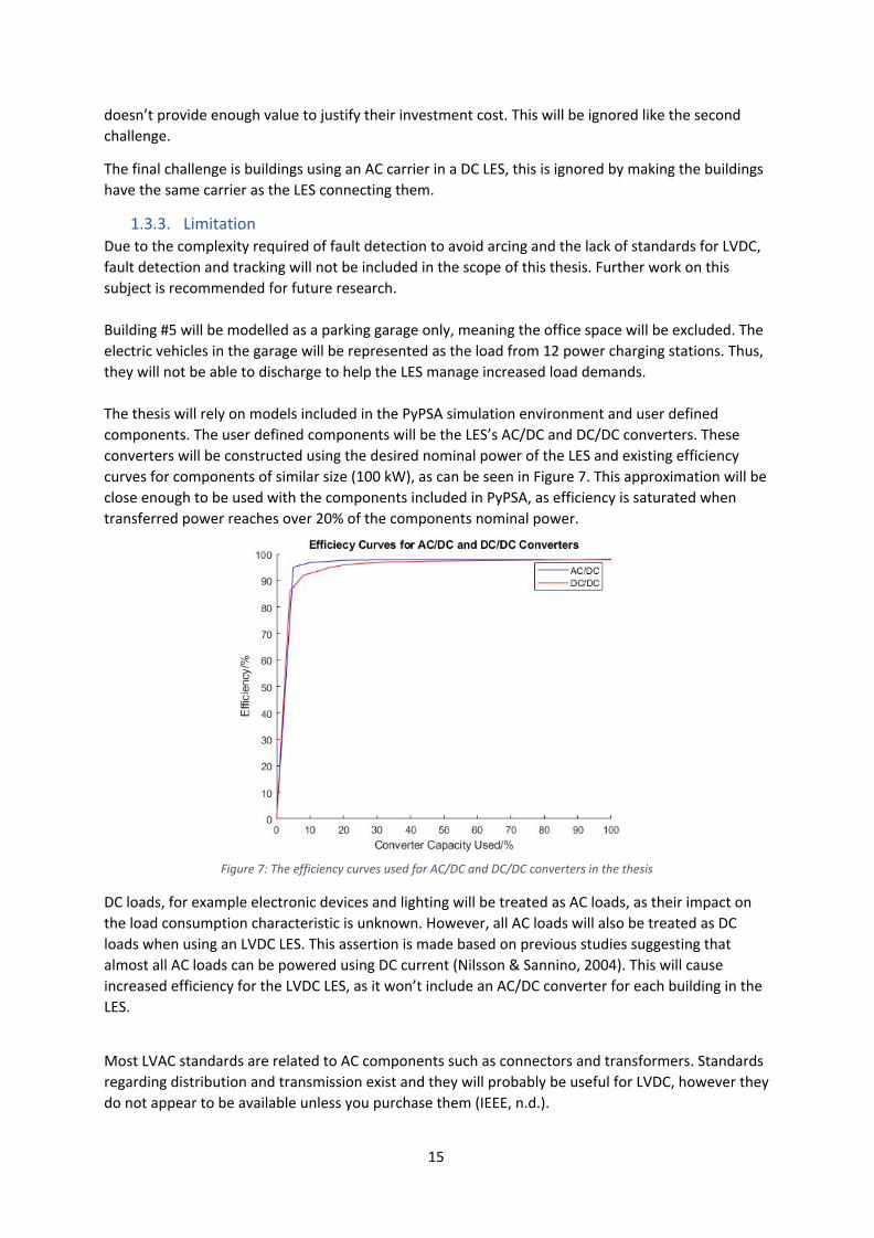
1.3.3. Limitation Due to the complexity required of fault detection to avoid arcing and the lack of standards for LVDC, fault detection and tracking will not be included in the scope of this thesis. Further work on this subject is recommended for future research. Building #5 will be modelled as a parking garage only, meaning the office space will be excluded. The electric vehicles in the garage will be represented as the load from 12 power charging stations. Thus, they will not be able to discharge to help the LES manage increased load demands. The thesis will rely on models included in the PyPSA simulation environment and user defined components. The user defined components will be the LES’s AC/DC and DC/DC converters. These converters will be constructed using the desired nominal power of the LES and existing efficiency curves for components of similar size (100 kW), as can be seen in Figure 7. This approximation will be close enough to be used with the components included in PyPSA, as efficiency is saturated when transferred power reaches over 20% of the components nominal power.

Figure 7: The efficiency curves used for AC/DC and DC/DC converters in the thesis

DC loads, for example electronic devices and lighting will be treated as AC loads, as their impact on the load consumption characteristic is unknown. However, all AC loads will also be treated as DC loads when using an LVDC LES. This assertion is made based on previous studies suggesting that almost all AC loads can be powered using DC current (Nilsson & Sannino, 2004). This will cause increased efficiency for the LVDC LES, as it won’t include an AC/DC converter for each building in the LES.

Most LVAC standards are related to AC components such as connectors and transformers. Standards regarding distribution and transmission exist and they will probably be useful for LVDC, however they do not appear to be available unless you purchase them (IEEE, n.d.).

15

2. Theory This chapter introduces relevant theory concerning the method and result of the thesis. The chapter will give the reader an understanding about the differences between AC and DC, as well as the components that are included in a LES. The chapter ends with stating the current situation regarding standardization of LVDC and the risk associated with it.

2.1. The difference between LVAC and LVDC Synchronicity

For two AC systems to interact with each other, both systems need to share the same voltage level and frequency. If components or systems lose synchronicity the different currents will start to interfere with each other and no power can be transferred between them. To make matching simpler the frequency of AC systems has been standardized to 50 Hz in Sweden.

DC doesn’t possess a frequency and has a steady voltage level, which makes it possible to transfer power between an AC and DC system by only matching the voltage level. Using a DC system in combination with an AC system also prevents desync, which can occur when using only AC systems. However, harmonic disturbances occur when converting DC to AC, which must be minimized by using a filter after the converter or a multilevel converter.

Difference in conversion losses

The difference in losses between an LVAC and an LVDC LES is where the AC/DC converters are located. In an LVAC LES AC/DC converters are necessary for solar panels and batteries, causing efficiency losses for all produced solar power and used battery power. Some losses can be mitigated by keeping both solar panels and batteries as part of the same LVDC system, letting the solar panels charge the battery without AC/DC losses.

In an LVDC LES all lines are DC based, allowing solar panels and batteries to power buildings through voltage regulation without the need for AC/DC conversion. Instead an AC/DC converter is needed to return power to or take power from an external AC grid. Depending on the self-sufficiency of the system, the losses from the AC/DC converter in an LVDC LES can exceed the removal of the solar systems AC/DC converters present in an LVAC LES.

Difference in cable losses

When an alternating current is run through a cable the moving electric charges will generate an alternating magnetic field, which causes an opposing alternating current. When this opposite current is run through the cable it forces the distribution current towards the outer shell of the cable, this is known as the “skin effect”. However, the skin effect is small for a 50 Hz LVAC LES and can be ignored (Luadani, 2018). The cables also have losses due to the reactive components that are present in the cable when alternating current is transported over long distances.

Because of the reactive AC loss, it’s more efficient to transport the current as DC since it doesn’t produce any of the two losses above. DC only causes resistive losses in the cables, which are also present when using AC. Resistive losses are the heat generated by running a current through a wire and is present in all electricity-based conductors. Resistive losses are sometimes called ohmic losses because of their relation to Ohm’s law, as all resistive losses are proportional to the formula

.RP r = * I2

16

2.2. Components As stated in 1.3. Limitations, all loads for an LVAC LES will be AC and all loads for an LVDC LES will be

DC. Based on this assumption Figure 8 shows an example of an LVAC LES and an LVDC LES.

Figure 8: Shows the topology of a LVAC (left) and a LVDC (right) LES.

The distribution busbar G1 of the LVAC LES is connected to an AC grid through a transformer. The busbar is in turn connected to the building’s busbar L2 through another transformer. If the system contains PV panels or an ESS, these will be connected to the LVAC LES through a DC/DC converter and an AC/DC converter.

The distribution busbar of the LVDC LES is connected to an AC grid through a transformer and an AC/DC rectifier. The busbar A can be connected directly to the DC/DC converters for PV panels and ESS. The distribution busbar is also connected to the building’s busbar through a DC/DC converter.

2.2.1. Transformer A transformer is used to step-up or step-down an AC’s voltage. It accomplishes this by placing two conductive windings around opposite ends of a metal core. When current is carried through the primary winding, it will generate a magnetic flux that travels through the core to the secondary winding. This will cause the flux to generate a current through the secondary winding. The windings and core can be seen in Figure 9. The size of the current in the secondary winding is dependent on the ratio between the number of turns in both windings. The voltage will step-down if the secondary winding has fewer turns than the primary winding and step-up if the secondary winding has more turns than the primary winding. The efficiency of a transformer is dependent on the amount of power being transferred through it. If the transformer is close to its maximum load, the efficiency will increase significantly (Schneider Electric, 2018)(Gouws & Dobzhanskyi, 2014).

The transformers in this thesis will therefore be dimensioned close to the maximum load value of the buildings. In 1.3. Limitations, it was decided that this thesis will use transformers that are included in the simulation program (PyPSA) and thus their efficiency is unknown.

17

Figure 9: The circuit diagram for a transformer.

2.2.2. AC/DC rectifier A rectifier is a power electronic component that converts AC to DC. The current can be converted through three diode bridge legs, where each phase is only allowed to pass through a leg if they clear a current threshold. Thereby making current with unintended amplitude unable to pass the leg. Both theleg and the conversion from sine-wave to a constant direct current can be seen in Figure 10. In Figure 10, the capacitor stores some power to try and keep the current at a constant level, which is why the DC doesn’t decrease with the AC phase sine-wave. In 1.3. Limitations, the efficiency for the rectifier is determined by using an efficiency curve. The efficiency of a power electronic rectifier is typically around 97% at over 10% power capacity.

Figure 10: Example of a rectifier.

18

2.2.3. DC/AC inverter An DC/AC inverter converts DC into AC, for example by passing the current through a transistor bridge with three legs. In Figure 11 the inverter leg contains an IGBT transistor in parallel with a diode on either side of the leg. Each leg will produce a different phase current with an alternating value. The value alternates since the positive and negative DC current is joined in each bridge.

The alternating voltage is decided using different control settings for the transistors and diodes. The simplest inverter type is a square wave inverter, as it will either release the full positive or full negative DC current. A slightly more advanced type is the modified sine wave inverter, where a zero value is added by letting both the positive and negative currents through at the same time. The modified sine wave inverter is commonly used for loads that don't require high power quality. The third alternative is the sine wave inverter, where an advanced inverter uses the DC currents voltage to simulate a sine wave, with Pulse-Width Modulation. The sine wave inverter is not used in distribution grids, since power quality is not that important due to the lack of sensitive AC loads.

The DC/AC inverters will be based on an efficiency curve with saturation at 98%, as stated in 1.3. Limitations. DC/AC conversion in distribution grids tend to have an efficiency between 96-98% (Rodrigo, Velázquez & Fernández 2016).

Figure 11: A circuit diagram of a DC/AC inverter.

2.2.4. DC/DC converter Like the transformer, a DC/DC converter can either step-down or step-up voltage, however it uses two different structures to do so. A DC/DC converter can either be a boost or buck converter. A boost converter increases the output voltage based on an inductor and the input voltage. A buck converter decreases the output voltage based on the input voltage and an inductor.

Figure 12 shows a circuit concept for a boost converter; the figure notably includes a switch and an inductor. When the switch is closed, the input current flows through the inductor generating a magnetic field. The magnetic field will store current and the input current will follow the path of least resistance through the switch. When the switch is opened, the current will decrease. The inductor will try to maintain the previous current and reverse its polarity to release the stored current. Since the inductor changes polarity, both the inductor and the input voltage will have the same polarity. As

19

both voltage sources are connected in series, their voltage will combine and the output voltage will be higher than the input voltage.

Figure 12: A circuit diagram of a boost converter.

Figure 13 depicts a concept circuit for a buck converter; this figure notably includes a switch, a diode and an inductor. When the switch is closed, current will flow from the input source through the inductor generating a magnetic field, allowing the inductor to store current. When the switch is opened, the inductor will attempt to keep the current flowing and reverse its polarity. The current released from the inductor will then flow through the load and the diode. This will decrease the output voltage, and thereby making the output voltage lower than the input voltage.

Figure 13: A circuit diagram of a buck converter.

2.2.5. Cables AC is transmitted using three phase currents A, B and C. The phase currents are alternating phase-shifted sinusoidal currents with a frequency of 50 Hz. DC is transmitted using a positive pole current, a negative pole current and a neutral current. The neutral current is created by combining the positive and the negative pole currents.

Several studies have been conducted regarding the need to replace the existing AC cables when building LVDC LES’s. (Taso, 2017), among others, found that it is possible to use existing AC cables to transmit DC current, as shown in Figure 14. AC and DC both use three partial currents and can therefore be transmitted through the same type of cables and thereby eliminate the need to replace existing AC cables.

The challenge of reusing existing AC cables is that DC current in LES’s can be run at a higher voltage compared to AC. Distribution LVAC has a voltage of 230 V, compared to LVDC which can use a voltage

20

of over 400 V. The maximum current that can be run through AC cables is the AC current’s phase-to-phase voltage. In Sweden the phase-to-phase voltage is 400 V, so LVDC with a voltage higher than 400 V cannot be run through the same cables.

As the thesis’ building site isn’t constructed yet, there would be no additional cost of replacing existing AC cables when building the LVDC LES. However, due to the conclusion drawn above LVAC and LVDC doesn’t have to use different cables, since the ambition of the thesis is to run load side LVDC at a voltage of 400 V. The AC or DC distribution grid connecting the buildings to the AC grid is run at 10 kV.

This thesis uses cables included in the PyPSA library, hence the losses of cables is handled by the program.

Figure 14: Shows how an AC cable can be used for DC.

2.3. Solar power Basic structure

Solar power is extracted through a Photovoltaic (PV) cell, which is a small semiconductor made from mono-or polycrystalline silicon. These semiconductors can absorb the power in solar irradiation and excite themselves to unbind their electrons, creating electron-hole-pairs. By exciting electrons and creating holes, a positive and a negative side are formed in the PV cell. Free electrons can travel as a current and therefore be used to transport the absorbed power of the PV cell through a grid.

If no external electric field is applied to the PV cell, the excited electrons will not have the power to cross the threshold region and lose their excited state when trying to push through the threshold region. By giving the electrons another path through the grid they can travel from the positive side of the cell to the negative side while powering the grid. To generate enough power, the cells are connected in series to form PV modules, which are subsequently series connected in PV strings. PV strings can be connected in parallel to form a solar panel. The solar panel can be connected to a grid and the excited electrons can transport the generated solar power from the PV cells to the electric loads in the grid (Bernardo, 2010).

At the build site, solar panels will be joined into several solar installations, which are placed on the roofs of the residential buildings and the parking garage. This thesis will be using data from an existing solar power installation and therefore no specific solar panel is used.

Solar irradiation

The solar power used for this thesis will be obtained by scaling the solar production from another existing solar installation to approximate the power generated from the solar installations on each of the buildings. The area of one installation has been specified by the building’s owner and the other installations areas are scaled based on this specification. The irradiation data will include one year of

21

solar production taking direct, diffuse and ground irradiation into consideration. The direct solar irradiation is the amount of irradiation that falls directly on the solar panel itself. The direct solar irradiation is the most impactful for solar production and the tertiary irradiation has the highest variance between locations.

The diffuse irradiation is dependent on the reflectance of the air and as such varies between locations. For an example (Kádár, 2016) found that in Hungary, at least 80% of the sun's direct beam irradiance passes through the atmosphere and therefore 20% becomes diffuse irradiation.

The ground reflected irradiation depends on the reflectance of the ground and the angle to the solar panels surface. Ground reflectance is dependent on the groundcover where the solar installation is located. For example, concrete has a varying ground reflectance for different mixtures of cement. In (Marceau & Van Geem, 2008) the highest reflectance of concrete is 69% for a crushed limestone mixture and the average for all mixtures is between 36-47%.

Self-sufficiency

In this thesis, the self-sufficiency of the LES’s is obtained by comparing the time the LES is completely unreliant on the AC grid (has solar overproduction), symbolized with TOver and the total number of hours the LES is studied, symbolized as TTotal;

elf uf f iciency S − s = TOverT Total

1)(

A high self-sufficiency is an important factor when estimating the profitability of a PV system, since using self-produced electricity is cheaper compared to using electricity imported from the AC grid. For this thesis E.ON is the most apt example, where a customer can sell to E.ON for 10 öre more than spot price (E.ON, 2019). This selling price will include government certificates for 3,5 öre/kWh , with a spot price that commonly ranges from 29 - 58 öre/kWh (Nordpool, 2020). In this thesis no individual installations will sell more than 30000 kr worth of electricity per year and therefore the owner will not get any sales tax on sold electricity and because no installation has more than 255 kW peak power the owners won't be required to pay the energy tax of 44,13 öre/kWh (Vattenfall, 2020)(Energimyndigheten, 2020). Thus the final sales price for electricity would be 41.5 - 61.5 öre/kWh. The building owners can also receive a 60 öre/kWh tax reduction for the first 30000 kWh they sell to the external grid (E.ON, 2019).

The owners of the buildings would have to pay the energy price of 45 - 68 öre/kWh (E.ON, 2020a) and the network costs of about 69 öre/kWh (E.ON, 2020b), which includes the energy tax and sales tax as well. Making the cost of purchased electricity between 114 - 137 öre/kWh. This makes batteries interesting, since it has been determined in (Enhörning & Odehed, 2018) that batteries can increase a microgrid's self-sufficiency by up to 22,9 percentage points.

2.4. Batteries (ESS) Basic structure

The basic structure of a battery consists of two electrodes, an anode and a cathode, separated by an electrolyte on either side of a separator. In Figure 15 the cathode, anode and separator are clearly labelled, and the electrolyte is the white area between each electrode and the separator. The electrolyte is a solution of one or more salts in one or more solvents and the separator is a porous membrane, both are used to prevent internal short-circuits. Short-circuits occur when the internal heat exceeds 60°C and leads to thermal runaway, during which the battery will catch fire. The

22

separator can stop this by expanding its porous structure to block ions from getting through at higher temperatures.

The most common battery for use in buildings and electric vehicles (EVs) is the lithium-ion battery. In a lithium-ion battery the cathode is made of lithium cobalt oxide and the anode is made of graphene. The separator is made of polyethene, common plastic, and the electrolyte is a mixture of lithium salts and an organic solvent. This thesis will use the Fronius solar battery 12.0 with 12 kWh capacity and 6,4 kW rated power tolerance (Fronius, n.d. b). The battery was chosen as it was the largest battery E.ON provides for residential solar installations.

Operation

Figure 15 will assist in illustrating the charge and the discharge of a battery. During charging an external circuit is applied. When the circuit is applied excited electrons move from the cathode, through the circuit to the anode. At the same time ions move from the cathode to the anode, through the electrolyte and the separator.

When discharging, an external load is applied to the battery. The excited electrons in the anode will move through the load circuit to the cathode, thereby powering said load. Meanwhile ions are transported from the anode to the cathode through the electrolyte and the separator.

Figure 15: Shows a battery cross section including the cathode, separator and anode. Also shows the direction of electrons during charging and discharging.

State of charge (SoC) is an indicator of how much of the battery's current capacity is filled. It is used as one of three key measurements for an ESS. The other measurements are the state of function (SoF) and the depth of discharge (DoD). The SoF is the measurement of how much power a battery can deliver during discharge, and will therefore be the supply limiter on an ESS. The DoD determines to what SoC the battery will be charged or discharged during each charge cycle, as seen in Figure 16. The DoD is one of the determining factors of the state of health (SoH) for a battery, the other being the battery's temperature. The SoH is the measurement of the charge capacity of the battery, hence if the SoH is decreased the battery drains its maximum SoC faster. With a DoD of 80%, the Fronius Li-ion battery would be able to perform 8000 cycles in its lifetime which is assumed to be 20 years (Fronius, n.d. b). An example of the DoD’s impact on total battery lifecycle can be seen in Figure 17. The temperature of the battery during operation will decrease the SoH faster than if the battery had been cooled.

23

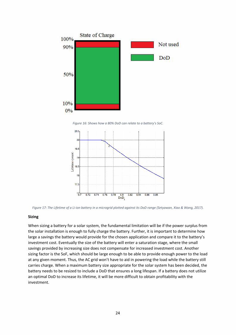
Figure 16: Shows how a 80% DoD can relate to a battery’s SoC.

Figure 17: The Lifetime of a Li-ion battery in a microgrid plotted against its DoD range (Setyawan, Xiao & Wang, 2017).

Sizing

When sizing a battery for a solar system, the fundamental limitation will be if the power surplus from the solar installation is enough to fully charge the battery. Further, it is important to determine how large a savings the battery would provide for the chosen application and compare it to the battery’s investment cost. Eventually the size of the battery will enter a saturation stage, where the small savings provided by increasing size does not compensate for increased investment cost. Another sizing factor is the SoF, which should be large enough to be able to provide enough power to the load at any given moment. Thus, the AC grid won’t have to aid in powering the load while the battery still carries charge. When a maximum battery size appropriate for the solar system has been decided, the battery needs to be resized to include a DoD that ensures a long lifespan. If a battery does not utilize an optimal DoD to increase its lifetime, it will be more difficult to obtain profitability with the investment.

24

2.5. Separated and interconnected LES The original intention of the building owners is to have each of their buildings connected to the AC grid without sharing power between them. In this case the buildings can be modelled as separate from each other and the buildings wouldn’t be able to share their solar production, instead any overproduction would be sold to the AC grid.

In the Eksta project examined in (Stierna, 2018), separate buildings were compared to an interconnected LVDC LES. The buildings had solar panels similar to this thesis’s buildings, so it can therefore be used to exemplify the increase of own-usage when comparing separate and interconnected LES’s. (Stierna, 2018) found that using an interconnected LVDC LES decreased the solar overproduction sold to the AC grid from 41% to 9%. The cost of purchasing electricity is higher than the price of selling electricity, as calculated at the end of section 2.3, so the more self-produced electricity a customer can use the more profitable the solar system becomes. This gives an indication that having the building owners interconnect their buildings into a common LVDC LES would increase the profitability of their building project. An interconnected LES would also make it possible to use the buildings batteries as one combined battery, further increasing own-usage and by thus self-sufficiency.

The difference between an interconnected and a separated LES is that there is no power shared between the buildings in a separated LES. Therefore, the power of separated cases are calculated based on the model in Figure 18. In Figure 18, the power is measured at the AC side of the AC/DC converter. In the figure, the interconnected case has one AC/DC converter for the whole LES and all the buildings are interconnected before the AC/DC converter. Due to this setup, the measurement will include all buildings loads, production and ESS. In the separated case, only one building is connected to one AC/DC converter. When the LES was simulated both these cases look identical, but are calculated as seen in the picture. The separated case calculates losses by partitioning the amount of power lost in the interconnected cases rectifier proportional to each building connected to it, thereby acting as if each building had a separate inverter.

Figure 18: A comparison between separately connecting the two buildings to a grid or interconnecting them.

25

2.6. Standards and Praxis

LVDC Standards

The IEC and IEEE are attempting to standardize LVDC, meaning that there are currently no standards available (Junpei, 2014). The ongoing standardization process revolves around updating LVAC and HVDC standards to include LVDC (IEC, 2017). Hence, most LVDC standards will be similar to the already existing standards for LVAC, with some exceptions taken from HVDC standards. One important standard that isn’t covered by this method is the LES voltage level, therefore the (IEC, 2018) technical report was created. The report details the standardization of voltage level through a survey conducted with different private and public actors in LVDC development.

Praxis for voltage levels

(IEC, 2018) defined that >48 V is used for interior lighting, 350-450 V is the voltage range for buildings in a LVDC LES and 600-900 V is also a possible voltage usable in LVDC LES’s. The survey determined that the preferred voltage levels in buildings was 380 V and 400 V. Further, the survey also determined that 750 V and 760 V were popular suggestions for LVDC distribution voltage. The most common voltage for MVDC in a distribution grid was 1500 V. (Sannino, Postiligione & H. J. Bollen, 2003) suggest using a voltage of 326 V for buildings, thereby allowing existing AC cables to be used when converting buildings into LVDC. Both newly constructed LVDC LES’s and converted LVAC LES’s should use 750 or 760 V to transfer power between buildings. The distribution grid in (Flyckt, 2018) used 760 V between the buildings according to the article (Norhstedt, 2017).

Preventing losses with increased voltage

In general power transfer has a higher efficiency when transmitted using higher voltage. Therefore, it is recommended to use the highest possible voltage for the power distribution in a LVDC LES. Increasing voltage will lower both the cable and conversion losses. The cable losses in a LVDC system are, as previously established, resistive losses. The resistive power losses are calculated using

, where the current squared is multiplied by the cable’s resistance. As the cable’sP = I2 * R

resistance is constant only the current can be varied. When the LES voltage is increased the current through the cable is reduced, since the power load in the LES is constant and is obtained using

. Therefore, increasing the LES voltage will reduce the current through the cables and thusP = U * I

reduce the cables resistive losses. The conversion losses are dependent on the load passing through the converter and the voltage of the converter system. Losses in a converter decrease when the load through the converter is high and when the voltage is high. To maximize efficiency the thesis LVDC distribution grid will use a higher voltage, 10 kV, and will be able to run through the same cables as a 10 kV LVAC distribution grid. The load side of the LES will run on 400 VDC and can be run through the same cables as the load side of the LVAC LES.

HVDC standards

As stated previously, the standards for HVDC and LVAC can be used as the basis for LVDC standards. The HVDC standard published in (IEEE,1997) tells how to test if a DC system can interact with an AC system, which could potentially be applied to LVDC. The standard also generally describes the process that should be used when testing an HVDC system on-site and off-site. The standard specifies a requirement to include harmonic filters on the AC side of an AC/DC conversion, as was stated in section 2.1. There are requirements for disturbance tests for both AC-system faults and DC-line faults. Lastly, it is stated that losses for an HVDC system should be computed at no-load and full load.

26

The standard exemplified here has the potential of being used for LVDC as it specifically focuses on testing and measuring a DC system interacting with an AC system.

2.7. Risks with LVDC The last chapter explained the situation regarding the lack of LVDC standards, which is the greatest risk when deciding to build an LVDC LES. The other important risk to consider is the protection systems and fault detection of the LVDC LES. These will be different from a LVAC system, since the faults present in an LVDC system are different from the faults in an LVAC system.

LVDC faults

In a DC system the DC fault leads to an increased current and rate of change for the current. The current at fault is limited by the LVDC systems converters, as opposed to LVAC systems where inductive impedance in the cables and the transformers serve as limiters. A hazardous fault in an LVDC system is the arcing fault, which does not self-extinguish when cancelled by an AC circuit breaker. As LVAC is an alternating system its faults will become zero once per period providing an opportunity for a fault to self-extinguish. As an LVDC system does not alternate this opportunity doesn’t exist, so the circuit breaker must possess arc interrupting capabilities. These capabilities are a magnetic arc blower and an arc chute, which combine to weaken and cool the arc until the arc exceeds the system's voltage and forces the current to become zero. In an AC system the current at fault will be over 10 times that of the nominal current making it easier to blow the arc into the arc chute. The current limiting caused by the DC system’s converters reduces the fault current to the extent that it does not trigger fault detection and may be too small to power the arc blower. By detecting these faults early, the complexity, power requirement and cost of the grid circuit breaker can be reduced (Cairoli & Dougal, 2013).

27

3. Method This section will detail the method used to obtain the results of the thesis. Starting with the dimensioning of the LES and followed by the data used in the simulations. Lastly, the simulation models for the case study are presented.

3.1. Dimensioning The nominal power of the system was determined based on the maximum power consumption of the four buildings’ loads and the garage load. The nominal power is applied to the power converters between the buildings and the distribution grid. Further, the converters to each buildings’ solar network are given a nominal power based on the size of the corresponding solar installations. Based on these parameters the converters between the LES and the AC grid have a combined nominal power of 1MW and the buildings’ solar subsections have a varying nominal power.

The battery size was only specified for Building #1, so the sizes of the remaining batteries have been determined by scaling the specified battery’s size to the remaining buildings, which can be seen in Table 1. Table 1 also shows how altering the size of the batteries between buildings, also changes the maximum charge-and discharge capacity. Depth of discharge is not affected by how many battery packs are attached to a building and therefore will remain as 80% and vary between 90% and 10% SoC.

Building Usable Capacity/kWh Maximum Charge/Discharge Power/kW

Building #1 67,2 44,8

Building #2 57,6 38,4

Building #3 28,8 19,2

Building #4 76,8 51,2

Garage 76,8 51,2

Table 1: A table detailing the capacity and power tolerance of each building's ESS.

The program calculates both the cable-and transformer losses for a chosen component in PyPSAs library. This model uses two different transformer models and two different cable types. The LES uses two transformer types as PyPSA doesn’t possess a model for a 1 MVA 10/0,4 kV transformer, hence the thesis model uses a 0,63 MVA and a 0,4 MVA 10/0,4 kV transformer for all AC-based models. The MVAC & MVDC parts of the LES’s use a 10,0 kV cable type and the low voltage parts of the LES’s are connected using a 0,4 kV cable type. All the components used in LES simulations are listed in Table 2.

28

Building Component Type Nominal power/kW

#1, #2 and #4 Transformer 0.63 MVA 10/0.4 kV 630

#3 and #5 Transformer 0.40 MVA 10/0.4 kV 400

All MVAC Cable 149-AL1/24-ST1A 10.0 210

All MVDC Cable 149-AL1/24-ST1A 10.0 210

All LVAC Cable NAYY 4x150 SE 210

All LVDC Cable NAYY 4x150 SE 210

Table 2: A table stating the PyPSA Type used by certain components in the simulation models.

3.2. In data The PyPSA models require two inputs to calculate the battery SoC and the power to-and from the AC grid. Both the PV production and the load data for each building on the site needs to be provided for each hour for a year, so seasonal differences can be observed and studied. The following subsections will present the two input variables and the summarised values over a specified period for each building.

3.2.1. PV production A solar installation in Hyllie provided by E.ON is the indata used for the solar production. The data is the hourly production from a 165kW solar installation for an entire year (16 April 2018 to 15 April 2019), which was rescaled for all the buildings’ solar installations. One of the two owners of Building #1 wanted to have a 160 kW solar installation on their part of the building. Then an assumption was made that all other buildings would have solar installations scaled to the buildings gross area, based on Building #1’s solar installation. The total production over the specified period is presented in the Table 3 below;

Year Building #1 /MWh

Building #2 /MWh

Building #3 /MWh

Building #4 /MWh

Parking Garage

Total yearly production/MWh

16 April – 15 April

113 101,7 52 131,1 131,1 528,9

Table 3: A table showing the yearly PV production of the different PV installations in the LES.

3.2.2. Load data The load consumption characteristic for each building is taken from a building of approximate size provided by E.ON. The load in the Building #5 doesn’t include the office load as stated in limitations. The load from the parking garage only includes EV-charging, as other loads are less significant in comparison and simplifies the load model. The one-year load characteristics of the garage are obtained from twelve EV charging stations, as stated in the limitations of this thesis. The total load consumption for each building over the specified period is presented in MWh’s in Table 4 below;

29

Year Building #1

/MWh Building #2

/MWh Building #3

/MWh Building #4

/MWh Parking

Garage/MWh Total yearly load /GWh

16 April – 15 April

762,2 741,9 398,4 834,1 760,1 3,5

Table 4: A table showing the total yearly power consumption of each building in the LES.

3.3. Scenarios and Models The simulation models for this thesis are constructed using Python and the library PyPSA. In PyPSA the LES is represented as a pandas DataFrame, a type of array. The network Dataframe contains the components added as array elements in a component DataFrame. A network is constructed using various components connected through buses and lines. The buses in the network control the voltage instead of the components, which are used to calculate efficiency losses.

The models use PyPSA’s type components for lines and transformers and user defined links as AC/DC and DC/DC converters. The links’ efficiencies are based on average efficiency curves for 100kW AC/DC converters and DC/DC converters respectively, which can be seen in Figure 7. The efficiency curves for AC/DC, DC/DC and transformers are all very similar at this high-power level, all averaging an efficiency of over 90% when loaded with 10kW or more power. Based on the building size the load will never fall below this point and so the only case where the higher component loses have a large effect on the result is during low PV production. All simulated networks use the in data specified in section 3.2.

Each type of network contains two different cases, one with batteries and one without, so in total there are eight different cases simulated. All eight models will be used to make a technical analysis between the cases based on how much power is needed from the AC grid. The eight models and their distinguishing attributes are shown in Table 5.

Case Number Topology Carrier type ESS

Case #1 Separated LVAC No

Case #2 Interconnected LVAC No

Case #3 Separated LVAC Yes

Case #4 Interconnected LVAC Yes

Case #5 Separated LVDC No

Case #6 Interconnected LVDC No

Case #7 Separated LVDC Yes

Case #8 Interconnected LVDC Yes

Table 5: A table describing the eight different cases to be simulated.

The following section will explain the method of building and running the cases from Table 5. Then the reason for why each individual case was chosen and what the goal of each simulation will be explained.

30

3.3.1. LVAC The topology of these cases can be seen in Figure 19. In these cases, the LES is connected to the buildings through two transformers, the transformer between G1 and the AC grid converts the grid HVAC at 130 kV to the AC distribution voltage of 10 kV. The transformers at buses M1 and M2 are the building transformers and convert the LES voltage to 400 V, which can be fed into the buildings. The solar installations DC subnetwork is connected to the load at the 400 V building buses (B1, B2…) on the load side of the transformer to avoid adding transformer losses to the solar power production. As his model is an AC network, the solar power needs to be converted to 400 V through a DC/DC converter and converted from DC to AC to feed into the AC distribution network. Since the AC grid transformer is present in all LES’s and therefore has no real impact on the comparison between the systems it is not included in the simulation. The DC/DC converter for the PV installation is included as the component efficiency for the solar generator in PyPSA, as the efficiency of the actual solar panels is already included in the PV installation in data used for the simulation.

As stated in the previous section, 3.2., there are no defined converter components in PyPSA and as such they must be approximated using links. Links are components that are placed between two buses in a chosen direction, where they act as load to their entry bus and generator to their exit bus. The problem with using the links in a simulation is that the links need to have the power going through them set as a variable instead of detecting the power at the link’s entry bus as the PyPSA transformer does. This means that a power flow simulation must be done to determine the power losses of the power at the entry bus going through the converter, to then set this power to the converter and then run the actual power flow calculation.

Figure 19: An overview of the LVAC simulation model's topology.

Figure 20 (the sequence diagram) below describes the process of executing the simulation for all LVAC cases, both with and without batteries. In Case #1 and Case #2 the sequence related to the battery control is omitted since no ESS is included. The general methodology revolves around circumventing the obstacle presented by the link components. As the link components need a set value for power to deliver any power through itself, a calculation must occur to determine the power

31

behind the link at the solar installations. These calculated values subsequently must be set as the power for the link and used to calculate the efficiency of the link. Then another calculation must be done to obtain the power from the links based on their set power and efficiency. When calculating the separated cases, the power loss from each building's cables is determined by comparing the combined results measured at each building with the result measured at the grid bus G1 and then distributing it in proportion to the power at each building bus.

Figure 20: A sequence diagram of what data is received from and given to the different simulations run on the LVAC models.

32

3.3.1.1. Scenario Case #1 - Separated This model was chosen to be the base case that all other cases are compared against, as it features a design lacking any of the tertiary components or technical alterations included in the other cases (interconnected buildings, DC carrier or batteries). To ensure the buildings had no effect on one another, all buildings were measured at each of their building buses (B#1, B#2, B#3, B#4 and B#5). If this LES model was used in an actual LES all the buildings would interact with each other since they are connected as in Figure 19, the owners would however measure and pay for the power as in the simulation. The goal with this model is to see how well the PV installation can provide power for each building without help from the surrounding LES. The result of the simulation will be measured at the buildings buses as stated previously.

3.3.1.2. Scenario Case #2 - Interconnected This case was made so all buildings would combine their PV production and show the difference in self-sufficiency of this LES compared to the LES in Case #1. This is accomplished by measuring the power at the unified grid bus G1 and having the buildings share their PV production with each other. It uses the same code as Case #1 but measures its result at the grid bus instead of at the buildings buses.

3.3.2. LVAC with ESS This model differs from the previous by adding a battery to each building's DC bus, which connects the PV installation to the DC side of the AC/DC converter as seen in Figure 21 below. The idea behind using a battery in a building is to only feed it using PV overproduction and therefore the batteries are placed as close to the PV installation as possible. This also removes the requirement to have an additional AC/DC conversion added between the PV installation and the battery, as would be the case if it was placed in the buildings internal LVAC load network.

Figure 21: An overview of the LVAC simulation model with ESS.

The sequence diagram in Figure 20 shows that to obtain the results from a LES model including batteries a few more code sequences must be implemented compared to Case #1 and Case #2. Firstly, the batteries need to be aware of when they can be charged or discharged, since PyPSA

33

doesn’t include such checks in their battery components. Hence, they must be fed the results from the previous simulations and use this to determine whether they can be charged or discharged.

To accomplish this the battery checks the result through several “if statements” to determine how much power is fed to or from the battery. An initial if statement checks if the LES is experiencing PV overproduction by noticing the sign of the power to the LES. The battery then decides if it can charge the battery based on the battery SoC and charging power tolerance. If the battery has a SoC over 10% and the LES starts to experience a load, the battery will discharge its SoC based on the load demand and the discharge power tolerance of the battery. The result of the battery control determines the increase or decrease of the SoC of the battery as well as what load/generation the battery contributes to the LES every hour.

In addition to the general battery control, Case #4 needs code for how the batteries are charged from other buildings in the LES. Since PyPSA does not have an internal control of when to charge and discharge a battery it also means that it is up to the user to define how the batteries interact with the larger grid and specifically the other buildings solar overproduction. To solve this an overproduction variable is created, which only holds a value during a single hour’s simulation before being reset. All overproduction is summarized and then distributed to one building’s battery at a time and charged until maximum hourly charge capacity is reached. This is done by subtracting the amount used to charge the batteries from the overproduction variable. The variable is also used to determine how many batteries need to be discharged for the load to become zero. Each battery in order from 1 to 5 uses as much of its stored power as possible to cover the load. If the charge is met the remaining batteries will not discharge.

Once the control function has determined what function the battery performs, the power of the batteries is set based on if the batteries act as loads or generators. Then the links are updated with the new occurrence that has happened in the DC subsystems. Thus, a new power and efficiency is set for the links, whereupon a new result is obtained from the grid bus G1.

3.3.2.1. Scenario Case #3 - Separated This case was made to see if the self-sufficiency of the LES can be increased by having the solar installations’ overproduction be used to charge batteries instead of sending it to the AC grid. As in the previous separated case, Case #1, it is interesting to observe how each building operates individually. Hence, the result is measured at each buildings’ building buses (B1, B2…) to isolate each buildings’ result from one another. This model's goal is to see if the LES can increase its self-sufficiency by charging each building with its own battery without help from the overproduction from other solar installations in the LES.

3.3.2.2. Scenario Case #4 - Interconnected One of the advantages with interconnecting buildings into a LES is giving the solar installations the ability to charge other buildings batteries. Thus, this model was created to study the difference in charging a battery with only one solar installation charging it versus while an entire LES’s worth of solar installations are charging all the buildings’ batteries together. The simulation will also show how multiple batteries work together to meet the load demand of all buildings in the LES instead of only meeting the load demand from the building they are attached to.

3.3.3. LVDC This model is built from the LVAC base model and it can be seen in Figure 22. To switch the network from AC to DC the transformers at M1 and M2 are replaced with DC/DC converters. To use DC/DC converters instead of transformers the LES’s charge carrier must be changed from AC to DC. To minimize power loss in the cables the PV installations are connected to the buildings buses as in the

34

LVAC case. It would be possible to attach the DC subnetwork to the high voltage side increasing the efficiency of the cables, however the efficiency would be lost due to the increased cable length and need for an additional DC/DC conversion. An AC/DC converter is added between the grid bus and the HVAC transformer at grid bus G1 to feed the DC LES. Furthermore, the building's loads have been replaced with DC loads as stated in limitations.

Now that no AC/DC converter is placed before the PV panels they can feed directly to the LES, however the load transformers have been replaced with DC/DC converters, which requires a second power flow to determine the losses at the load. Afterwards a third power flow is needed to determine the losses of the LES’s AC/DC converter. The program requires a generator to perform a power flow on a subsystem, which wasn’t a problem in the LVAC cases as there was only the PV subsystem with a PV generator included. However as stated the LVDC system has a DC/DC converter modeled as a link sitting between the AC grid and the load, this creates a subnetwork at the load. Since the load subnetworks doesn’t contain any actual generators, a dummy generator must be inserted into each load subnetwork.

Figure 22: An overview of the LVDC simulation model.

The simulation of this model is like the other separated cases where the result is measured at the building buses (B1, B2…). However, the simulation's first power flow now determines each building’s load consumption, which is then set as the power of the buildings’ DC/DC converters as can be seen in Figure 22. The DC/DC converters are represented as DC link components in PyPSA, which functions as a load at the entry bus and a generator at its exit bus. So, if a load value is to be transferred through the converter the power applied to the converters must be negative. Hence the power set for the DC/DC converters is the negative load value of their respective buildings for every hour. The power transferred through both DC/DC converters will then be set as the power of the AC/DC converter and used to calculate its losses. After that another simulation is run to determine the result, which can be measured at bus G3. As in the AC cases, when calculating the separated cases the power losses are determined based on the combined power of the separated buildings buses and the total power at the grid bus G3.

35

Figure 23: A sequence diagram of what data is received from and given to the different simulations run on the LVDC models.

36

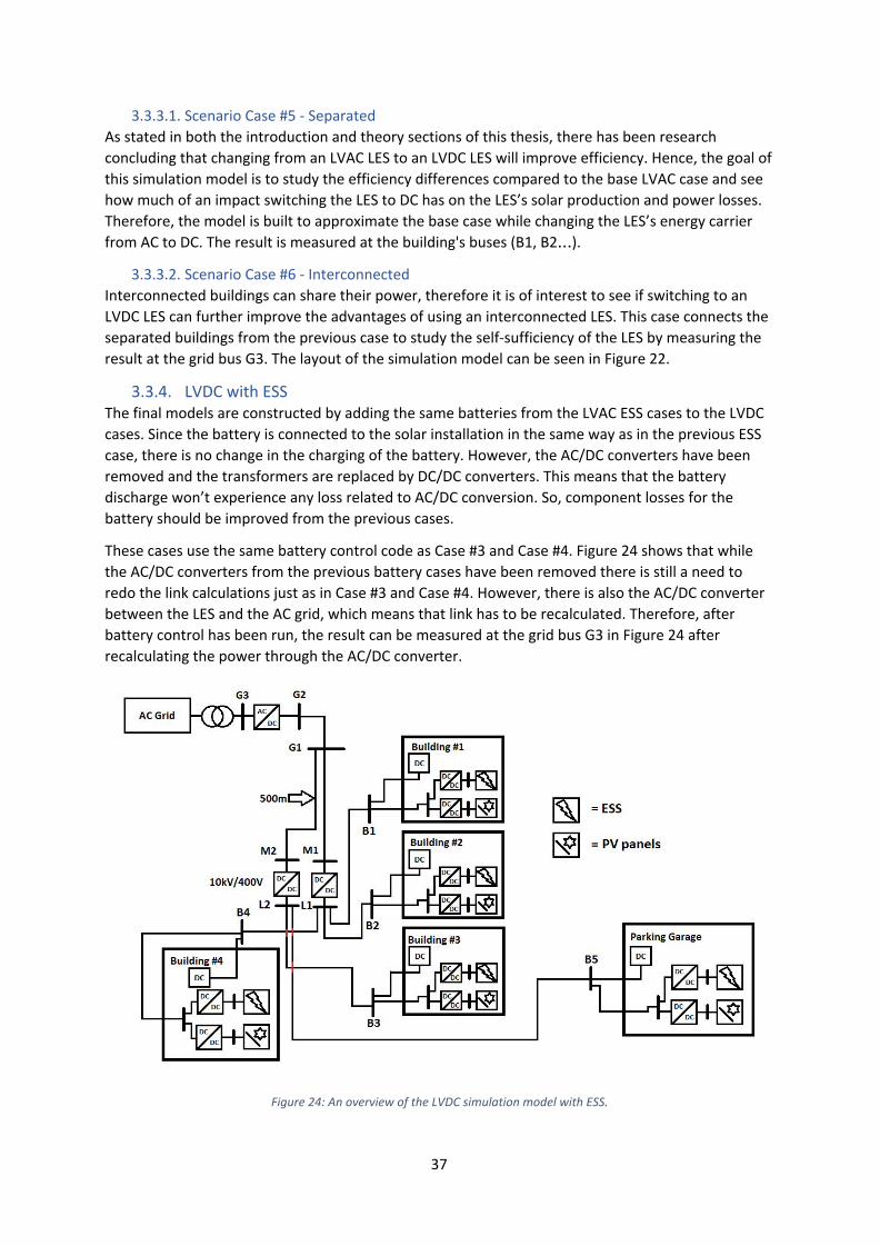
3.3.3.1. Scenario Case #5 - Separated As stated in both the introduction and theory sections of this thesis, there has been research concluding that changing from an LVAC LES to an LVDC LES will improve efficiency. Hence, the goal of this simulation model is to study the efficiency differences compared to the base LVAC case and see how much of an impact switching the LES to DC has on the LES’s solar production and power losses. Therefore, the model is built to approximate the base case while changing the LES’s energy carrier from AC to DC. The result is measured at the building's buses (B1, B2…).

3.3.3.2. Scenario Case #6 - Interconnected Interconnected buildings can share their power, therefore it is of interest to see if switching to an LVDC LES can further improve the advantages of using an interconnected LES. This case connects the separated buildings from the previous case to study the self-sufficiency of the LES by measuring the result at the grid bus G3. The layout of the simulation model can be seen in Figure 22.

3.3.4. LVDC with ESS The final models are constructed by adding the same batteries from the LVAC ESS cases to the LVDC cases. Since the battery is connected to the solar installation in the same way as in the previous ESS case, there is no change in the charging of the battery. However, the AC/DC converters have been removed and the transformers are replaced by DC/DC converters. This means that the battery discharge won’t experience any loss related to AC/DC conversion. So, component losses for the battery should be improved from the previous cases.

These cases use the same battery control code as Case #3 and Case #4. Figure 24 shows that while the AC/DC converters from the previous battery cases have been removed there is still a need to redo the link calculations just as in Case #3 and Case #4. However, there is also the AC/DC converter between the LES and the AC grid, which means that link has to be recalculated. Therefore, after battery control has been run, the result can be measured at the grid bus G3 in Figure 24 after recalculating the power through the AC/DC converter.

Figure 24: An overview of the LVDC simulation model with ESS.

37

3.3.4.1. Scenario Case #7 - Separated By adding batteries to the model in the separated LVDC LES, it would be possible to lose less solar overproduction to efficiency losses and discharge the batteries more efficiently. The purpose of this model is to see how much energy is saved by using batteries compared to the separated LVDC case and how much the overall LES efficiency and battery usage is increased by switching from LVAC to LVDC. The result is measured at the buildings' buses (B1, B2…)

3.3.4.2. Scenario Case #8 - Interconnected The goal of this simulation is the same as the goal of Case #4, in that it seeks to further improve battery charging in comparison to its separated battery case by letting the buildings in the LES help charge each other’s batteries. This case will also attempt to demonstrate its overall LES efficiency compared with its corresponding LVAC case. The result is measured at the grid bus G3.

3.3.5. Comparison The comparison of technical performance will include how efficient power transfer is through the LES, the batteries performance and the LES's self-sufficiency. The overproduction is a variable that will be considered in the comparison since it would, based on the literature studied, increase the profitability of the system. Even if no financial analysis is conducted on the system the fact that more power transported to the AC grid would have a positive effect on the cases commercial viability will still be useful to the comparison. This stems from the same reason that self-sufficiency is an important technical benchmark for the LES cases. Previous studies have shown that it is a critical variable in commercial analysis and thus future work needs to be done in this area.

38

4. Results The results of the case study simulations are presented in this chapter. First, the powerflow simulation for each hour from 15th April 2018 to 15th April 2019 is shown as line graphs for Case #1. The LVAC and LVDC versions of each case type won’t be presented individually, as they look too similar to spot any differences between them. Instead the differences between the cases are shown in line graphs following the Case #1 line graph.

As can be seen in Figure 25, the buildings are being supplied from the AC grid for most of the year. It is during the months of April-August where the solar production can exceed the load demand and give overproduction. The figure makes it clear that should batteries be added it is during this time they will be usable and it is apparent that the batteries won’t be able to charge at all during winter.

Figure 25: Resulting powerflow of every building in the LVAC LES at every hour for one year. The negative power values are overproduction and the positive are supplied by the AC grid.

4.1. Scenario Case #1 and Case #5 Figure 26 shows the difference between Case #1 and Case #5, where positive values indicate losses when using the AC case instead of the DC case and negative values indicate the energy savings. The figure shows that during the year there is a majority of losses from using the LVAC LES instead of the LVDC LES. However during the times where the LVAC LES has energy savings compared to the LVDC LES these savings are larger than the LVAC LES’s losses for an average hour. This does not help as the majority of the time the LVAC LES is losing power compared to the LVDC LES. Between October and February there is not a single time any of the buildings have energy savings when run on LVAC instead of LVDC. For a majority of the year the AC grid losses are between 0,5-5kWs of power per hour. Each building has a fairly similar difference of power since they all have the same solar production pattern and mainly differ in load profile.

39

Figure 26: Resulting differences in powerflow of every building in the LVAC LES and LVDC LES at every hour for one year. The negative power values are power savings and the positive are the power losses, when using LVAC instead of LVDC.

4.2. Scenario Case #2 and Case #6 The figure below show the differences in the powerflow simulation of Case #2 and Case #6 at every hour for one year. As stated in the method chapter these powerflows were obtained by measuring the results of Case #1 and Case #5 at the grid bus instead of each building’s bus. The interconnected LES’s have solar overproduction between March and September, thus it is entirely grid supplied for the remaining months. This is consistent with Case #1 (Figure 25) and Case #5, thus interconnecting the LES’s doesn’t increase the months that overproduction occurs. Therefore, interconnecting the LES’s changes the own-usage of overproduction, not the amount of hours of overproduction.

The graph in Figure 27 is similar in pattern to the separated graphs in Figure 26 and shows that interconnecting the LES’s does not make the interconnected LVAC case (Case #2) more viable than the previous LVAC case (Case #1). As in the previous figure there is no point in which the LVAC case gives any energy savings during October to February. This can be used to show that the LVDC cases provide increased efficiency over the LVAC cases.

40

Figure 27: Resulting differences in powerflow from the interconnected LVAC LES and interconnected LVDC LES at every hour for one year.

4.3. Scenario Case #3 and Case #7 Figure 28 show the difference in the results of the powerflow simulations of Case #3 and Case #7. The difference from the previous separated cases is the inclusion of batteries. The batteries cause a reduction in overproduction between 19 and 51 kW per hour depending on the building. As buildings can exceed over 100 kW of overproduction the batteries can be filled in 2 hours during summer and thus their impact is seen as brief spikes in the figures. If this figure is compared to Figure 26 it is apparent that the losses for the LVAC case (Case #3) has increased compared to the LVDC case (Case #7). This could be caused by the power losses in the LVAC case making it take longer to charge the batteries of the buildings and thus causing sudden spikes in power difference, as the LVDC case can start giving overproduction to the AC grid while the LVAC case is still charging.

Figure 28: Resulting difference in powerflow of every building in the separated LVAC LES with batteries and the separated LVDC LES with batteries at every hour for one year.

41

4.4. Scenario Case #4 and Case #8 As in the previous interconnected cases, the powerflows being compared in Figure 29 were obtained by measuring the powerflow of Case #3 and #7 at the grid bus instead of the building’s buses. The change from Case #2 and #6 is including batteries in the model. The batteries have a combined DoD of 205 kW, therefore the same spikes that occurred in the previous figure are in this figure as well. Comparing this figure to Figure 27 shows a large increase in losses for the LVAC case due to the charging spikes. These spikes are so large that it makes it harder to see the losses on an average day even though these losses vary between 1-20kW.

Figure 29: Resulting differences in powerflow from the interconnected LVAC LES with batteries compared to the interconnected LVDC LES with batteries at every hour for one year.

4.5. Efficiency and load demand for the AC grid Figure 30 shows the amount of load demand that was covered by the AC grid and thereby shows how much each case changes the energy savings of the LES. In Case #1, the yearly load demand provided by the AC grid was 3,22 GWh and the highest load demand from the AC grid off all cases. Case #8 has the lowest load demand covered by the AC grid at 3,11 GWh, which makes the difference between Case #1 and Case #8 is 3,5%. Also notable is that changing Case #1 to Case #5 (LVAC to LVDC) caused an increase in energy saving 1,6% of energy from the AC grid, which is due to increased efficiency. The cause of this change is seen in the powerflow figures in the previous subsections, where the LVDC cases have lower losses than the corresponding LVAC cases. The use of batteries lowers the amount of energy required for the AC grid by storing the unused solar power, as seen in Figure 30 where Case #3 has a lower amount of power supplied by the AC grid than Case #1. The final cause of lower power demand from the AC grid is interconnecting the buildings in the LES, which allows the overproduction from one building to help fill the load demand of other buildings in the LES. In Figure 30 there is a noticable difference between the LVAC cases and the LVDC cases, Case #6 has lower power demand from the AC grid than Case #7. This differs from Case #2 and Case #3, where Case #2 has more load demand from the external grid. The conclusion that can be drawn from this is that interconnecting buildings is more effective in the LVDC LES than the LVAC LES.

42

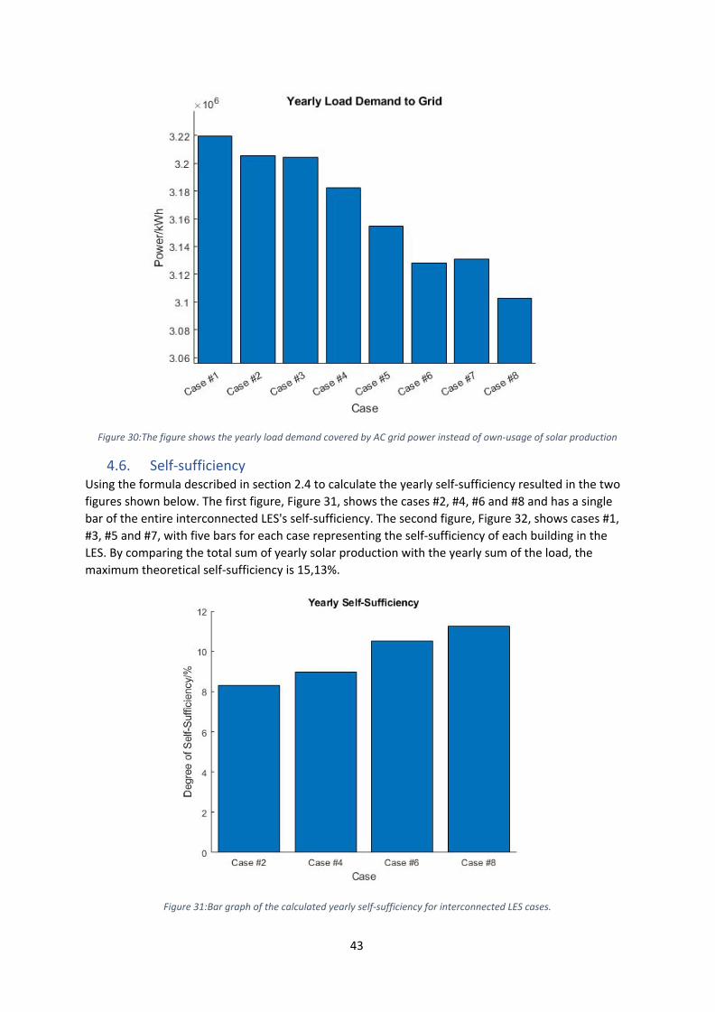
Figure 30:The figure shows the yearly load demand covered by AC grid power instead of own-usage of solar production

4.6. Self-sufficiency Using the formula described in section 2.4 to calculate the yearly self-sufficiency resulted in the two figures shown below. The first figure, Figure 31, shows the cases #2, #4, #6 and #8 and has a single bar of the entire interconnected LES's self-sufficiency. The second figure, Figure 32, shows cases #1, #3, #5 and #7, with five bars for each case representing the self-sufficiency of each building in the LES. By comparing the total sum of yearly solar production with the yearly sum of the load, the maximum theoretical self-sufficiency is 15,13%.

Figure 31:Bar graph of the calculated yearly self-sufficiency for interconnected LES cases.

43

It is apparent that adding batteries increase the self-sufficiency of the LES in both the LVAC and LVDC cases as Case #4 is more self-sufficient than Case #2 and Case #8 is more self-sufficient than Case #6. Based on this bar graph it can also be determined that Case #6 is 25% more self-sufficient than Case #2 and that Case #8 is 23% more self-sufficient than Case #4.

Figure 32: Bar graph of the calculated self-sufficiency for each building in the separated LES cases.

Figure 32 shows an average increase in self-sufficiency when adding batteries to both the LVAC and LVDC LES, when comparing Case #1 with Case #3 and Case #5 with Case #7. Comparing Case #5 and Case #7 with Case #1 and Case #3 shows that the LVDC LES’s have a higher base self-sufficiency than the LVAC LES’s. This can be seen by comparing how much the overproduction is reduced between the mentioned cases. The difference between Case #1 and Case #3 is ~33%, while the difference between Case #5 and Case #7 is ~26%. As all cases use the same battery size and solar production the amount of overproduction available reflects the usage of batteries and the losses in the LES.

44

Figure 33: Bar graph of the calculated overproduction sold to the external grid each year for all LES cases.

The overproduction sold to the AC grid is shown in Figure 33. The figure makes it clear that changing the LES from being AC based to DC based increased overproduction. Notably, Case #6 has significantly higher overproduction compared to Case #2, while the other LVDC cases seem to have a similar percentage increase from conversion. This happens because the efficiency increase in the solar production in Case #5 is mostly happening when there is already a surplus from the buildings, so interconnecting them doesn’t increase own-usage of the overproduction as much. When looking at all cases it is apparent that adding batteries and interconnecting buildings decreases the amount of overproduction.

4.7. Energy storage The amount of hours the batteries are active is shown in Figure 34 and is used to clearly illustrate how much each case has used at least one building’s battery. Figure 34 makes it clear that the separated cases have more usage out of at least one buildinings battery at any given hour of the year. Charging batteries with an interconnected charge control caused a 37% reduction in overall battery activity in Case #4 and a 36% reduction in Case #8. This is caused by two factors, one is that the interconnected cases use overproduction to help charge other buildings. The other factor is that the batteries of the LES are interconnected, which means they can use all their stored charge to help alleviate one building’s load whenever there is a building that can’t cover its load with solar power. This causes the interconnected LES’s batteries to not store power or hold on to their SoC as long as the separated LES’s batteries.

Figure 35 shows how many hours per year all batteries are fully charged, the figure shows that the interconnected cases can fully charge all the batteries more than the separated cases. Case #4 and Case #8 charges all batteries to full capacity almost twice as many hours per year as Case #3 and Case #7. Case #3 is fully charged 52% as much as Case #4 and Case#7 is fully charged 54,5% as much as Case#8. From the figure it becomes apparent that interconnecting the LES causes a large increase in the batteries’ ability to attain full charge. The figure also shows an overall increase in this ability, when using an LVDC LES instead of an LVAC LES.

45

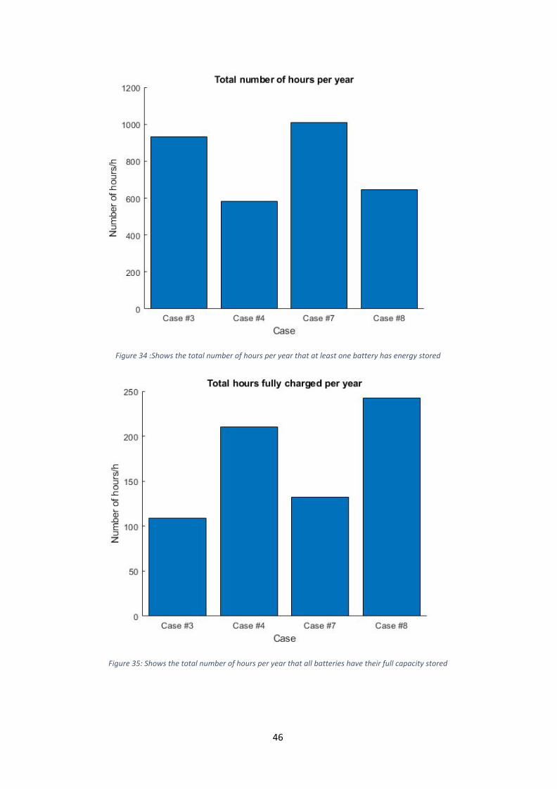
Figure 34 :Shows the total number of hours per year that at least one battery has energy stored

Figure 35: Shows the total number of hours per year that all batteries have their full capacity stored

46

5. Analysis This section is dedicated to analyzing the results from the case study and how the cases perform in comparison with each other. This discussion will evaluate the results of the case study based on the technical aspects that were to be studied, as stated in this thesis purpose. This discussion will serve as the foundation for the conclusion of this thesis, which can be found in the next chapter.

5.1. Result of battery simulation The result of the simulations showed that adding batteries increases the self-sufficiency of the LES. The overproduction graph in Figure 33 made it apparent that the DoD of the batteries isn’t large enough, as overproduction remained unused. Thus, it would be possible to install larger batteries than the building owner specified, in order to get a higher self-sufficiency for the LES cases that include batteries. During summer the overproduction is large enough to charge batteries that are three times larger than the current ones. The problem with increasing battery size is that the cost and payback time of batteries are not included in the thesis. This is important, since past research has shown these factors to be vital in determining the commercial viability of batteries. (Flyckt, 2018) determined that although batteries provide an increase to self-sufficiency and thereby reduce the amount of power purchased from the AC grid, it is not worth the investment. The batteries used in this thesis are many times larger than in (Flyckt, 2018), however they do not provide the levels of self sufficiency increases seen in (Enhörning & Odehed, 2018) and thus there is a risk that their inclusion would be detrimental to a commercial project. Therefore, it is difficult to make any recommendation on using larger battery sizes in commercial LES cases as it might not be economically viable, even if it increases self-sufficiency.

By using batteries the overproduction sold to the AC grid can be reduced as seen in Figure 33. The reduction in overproduction by adding batteries to a LES can be seen below. From the table it is apparent that inserting batteries in the LVAC cases gives a greater reduction in overproduction than inserting batteries in the LVDC cases. The variation in reduction can be partially explained by the increase in overproduction between LVAC and LVDC. The result also points to the batteries not being large enough to take advantage of increased overproduction, as Figure 33 shows that the LVDC cases have more overproduction than the LVAC cases overall. This is further proof that the batteries need to be larger to fully utilize the LES’s overproduction.

Cases Case #1 to Case #3 Case #2 to Case #4 Case #5 to Case #7 Case #6 to Case #8

Percentage reduction

32,9% 30,8% 26,3% 28,9%

Table 6: The table shows the percentage reduction in overproduction when adding batteries to a LES case

5.2. Overproduction The powerflows shown in Figure 25 reveals that the solar production is able to cover the load demand of the LES during the day, most days in late spring and during the summer. The overproduction doesn't cover the load demand often or at all during the rest of the year.

The Xiamen University project concluded that their solar production wasn’t enough to cover air conditioning and EV-charging with 150 kW of installed solar panels. As the powerflow simulation shows, there is not enough solar power to power all the buildings for most of the year. Some of this is caused by the seasons in Sweden, but a part of it can be explained by the conclusion of the Xiamen study. Even if more solar power was installed in this thesis’s LES cases there might be more consistent battery charging if solar production was used to cover certain loads and let the AC grid power the rest, as the LES cases can’t become islands anyway. The usage of batteries would increase,

47

as there are days in spring and autumn where the solar panels are producing power but not exceeding the load demand for the entire building and thus not charging the batteries. This would also allow the batteries to discharge over longer periods of time as the load they would have to cover every hour would be lower. Meaning, that their size could be smaller than if they have to cover the entire building's load.

Since the thesis doesn’t include an economic analysis, factors such as selling increased overproduction cannot be properly considered. Not selling overproduction benefit cases with batteries, because self sufficiency and efficiency are the variables used to compare the results of the case study. As the study stands, the battery cases (Case #2, Case #4, Case #6 and Case #8) have the same efficiency and higher self-sufficiency than their counterparts. Thus, the conclusion will be based on the result that batteries don't lower the efficiency of the LES and increase own-usage of solar overproduction, which increases self-sufficiency.

5.3. LVAC vs. LVDC The LVDC LES has increased the efficiency of both PV systems and batteries by removing the AC/DC conversion required in the LVAC LES, as seen in Figure 31. By doing so the LVDC cases have higher overproduction and gain more potential to increase the own-usage of solar production. Hence, why the later LVDC cases have better self-sufficiency than their LVAC counterparts. As noted previously, even if overproduction increases there isn’t enough battery storage to utilize this overproduction to increase the own-usage significantly.

Transitioning from LVAC to LVDC has increased overproduction as seen in Figure 33. This is due to the increased efficiency of the buildings’ solar subsystem and decrease in conversion losses to the load. In the result it was pointed out that Case #6 had a greater increase in overproduction than the other cases. This happened due to the low battery capacity that was discussed previously, as there is more solar production which fills the buildings battery rapidly and then has to sell the rest. In Case #8, the overproduction is lowered similar to the reduction in batteryless cases, meaning that interconnecting buildings allowed the buildings to use their overproduction to charge other buildings batteries. The reduction of overproduction in going from Case #5 to Case #6 is 48% of the reduction when going from Case #1 to Case #2. The reduction of overproduction going from Case #7 to Case #8 is 92% of the reduction when going from Case #3 to Case #4.

The transition from AC to DC has also decreased the load covered by the AC grid. However, it should be noted that any current LVDC LES would lose some of this advantage as commercial buildings would probably remain as AC and would require a DC/AC inverter.

This condition can be used to create a possible case for future research, such as interconnecting the solar subsystems of each building while the LES uses LVAC. In this case there would be no conversion between different buildings solar panels or batteries. Therefore the solar subsystem would retain increased efficiency when transferring power between buildings present in the interconnected LVDC cases (Case #7 and #8). There would be a conversion loss between the combined solar subsystem and the LVAC LES. However, since the LVAC cases (Case #1-#4) would have more conversion losses in its solar subsystems and the same losses in its distribution system, there is reason to hypothesize that this case would be more efficient than the LVAC cases. This could also make it more efficient than the LVDC cases, given that the buildings were AC-based instead of DC-based.

48

5.4. Separated vs. Interconnected The powerflow results in figures 26-29 combined with the total load covered by the AC grid in Figure 30 shows that interconnecting buildings decreases the amount of power required from the AC grid. Interconnecting LES’s reduce the power required to a similar extent as adding batteries to the separated buildings, by 0,5% in the LVAC cases and 0,85% in the LVDC cases. By interconnecting and adding batteries to Case #1, 1,2% less power had to be supplied by the AC grid and doing the same to Case #5 results in a 1,65% reduction. The result shows that interconnecting the LES only reduces the power that needs to be supplied from an external grid by less than a percent.

Figure 33 is more helpful when discussing the benefits of interconnecting the LES buildings , as it shows a notable reduction in overproduction by interconnecting the buildings. Interconnecting Case #1 to create Case #2 caused a 16,2% reduction in overproduction sold to the AC grid and interconnecting Case #5 to create Case #6 caused a 7% reduction in overproduction. This result shows that own-usage is increased by interconnecting the LES and thus is an argument for using interconnected LES’s when the system contains solar power production. The LVDC case having a lower reduction than the LVAC case is consistent with the previous analysis on the overproduction. The reason for the decreased reduction is due to the increased overproduction from each building in the LVDC case covering the buildings load to a larger extent than in the LVAC case. This leads to the conclusion that to utilize the benefits of interconnecting the LES, batteries should be added.

5.5. Battery interconnection Interconnecting a LES with batteries had a less clear cut result than the other parameters. Figure 34 shows that the interconnected cases have less hours of battery activity than their separated counterparts. The reason Case #4 and Case #8 have lower overall activity for batteries stems from the increased usage of overproduction as can be seen in Figure 33. In Figure 35 it becomes apparent that the interconnected cases can bring the batteries to full capacity more often than the separated cases. This is due to the control scheme used to charge the batteries in these cases.

The interconnected cases (Case #4 and Case #8) are charged to full in order from Building #1 to Building #5, thus the batteries will reach maximum charge capacity more often than in the separated cases. In the separated cases any buildings overproduction is used to charge that building's battery and is then fed to the external grid.

The result shows that interconnecting a LES with batteries makes it possible to charge the batteries to full more often than the separated LES, meaning the interconnected cases would benefit more from increased battery capacity than the separated cases. As stated before, it is recommended to increase battery capacity and to also use a few larger batteries instead of five batteries in the interconnected cases, as this would lower their cost. Due to the result in Figure 34 it would also be recommended to increase the amount of solar production in the interconnected cases as they don't have enough solar production to cover the buildings loads and properly utilize the batteries.

5.6. Standards and voltage level The results were obtained by using the same voltage for both LVAC and LVDC LES’s. This was done in order to make the comparison as fair as possible, since the question wasn’t if increasing voltage would increase efficiency. It was also decided that the distribution grid would be run at 10 kV for both AC and DC cases for the same reason. There is an argument for using 700 V in an LVDC LES as it would be more efficient than using 400 V, as there is no established voltage level standard for LVDC LES’s. But using this voltage level would inevitably bring up the question if LVAC would be more efficient than this LES if the LVAC LES had the same voltage level. As LVDC LES’s would only be used

49

locally and this study uses a LES connected to the LES, it would be just as easy to make a 700 V LVAC LES as a 700 V LVDC LES.

In the case where buildings are kept at the standard LVAC voltage, a case where all solar subsystems are interconnected has been suggested. In this case it would be possible to increase the voltage level of the solar subsystem to increase transfer efficiency between the buildings. This could help increase the overall usage of solar overproduction as the distances between the buildings are long enough to have an impact on the usable solar production, due to cable losses.

5.7. Losses In this case study there are notable differences between each case and thus the losses for the cases as well. To analyze the losses of the different LES cases they will be divided into four categories; always present, LVAC, LVDC and battery losses.

The losses that are always present are the cable losses and the DC/DC conversion losses for solar power. There is also a transformer loss from the transformer that connects the LES the thesis studies to the AC grid, but since it is outside the LES it isn’t included in the case simulations. As for cable losses, they are handled by the program as described in the method. The DC/DC converters for the solar power installations have losses based on the DC/DC efficiency curve, that was mentioned in the method chapter. The DC/DC efficiency curve starts to saturate at 5% of its nominal power. There are a few times a year where the solar production is small enough that these low power efficiencies are used, in which case the losses are at around 60-40%.

In the LVAC cases the additional losses are the transformers and the AC/DC converters for the solar installations. As stated in the methods the transformers are controlled by the simulation program, but they appear to follow a similar efficiency curve to the converters. The AC/DC converters have an efficiency curve that starts about 4 percentage points lower than the DC/DC converters efficiency curve. The AC/DC converters curve starts increasing by about 4 percentage points faster than the DC/DC converters efficiency curve once they hit 5% of nominal power. They both plateau at almost 99% efficiency when they are close to nominal power.

The LVDC LES replaces the LVAC LES’s transformers with DC/DC converters and removes the LVAC LES’s AC/DC converters at the solar installations. The LVDC LES also adds one AC/DC converter at the end of the LES to convert the AC grid’s input/output to the proper carrier. The DC/DC converters operate on the same efficiency curve as those in the solar installations and the AC/DC converter uses the same efficiency curve as the LVAC LES cases AC/DC converter.

When batteries are added into either LVAC or LVDC LES’s there is one DC/DC converter loss added to each solar installation subsystem, for the converter to the batteries. This converter is only used when the battery is charging or discharging and operates at a high efficiency. The high efficiency comes from the converter being sized for the batteries input/output and the solar production and loads being large enough to require the converter to work at nominal capacity. The second effect on the losses is that the battery can bring the overall powerflow in the LES to near 0, meaning that both converters and transformers are working at very low efficiency. Though the effect of these losses aren’t that significant since the powerflow through the LES is so low.

The results showed that having less converters in the LES resulted in lower overall losses for both solar production and load only hours. The result also showed that moving converters out of the LES helps increase the benefit of having interconnected LES’s. The conclusion that can be drawn from this is that to prevent extraneous losses there should only be enough converters in an interconnected system to allow it to function at the same voltage level and carrier.

50

6. Conclusion & Future Work

The purpose of this thesis was to determine which case in the case study was most efficient and self-sufficient. In doing so it would also conclude if interconnecting buildings, adding batteries to a LES and changing a LES from LVAC to LVDC could improve upon these qualities.

6.1. Conclusion LVAC and LVDC

The result of the case study points to the use of LVDC for a LES will increase self-sufficiency and overproduction from solar installations. The increase of self-sufficiency was less than expected due to solar production being too low to supply the load demand for much of the year. This leads to an uncertain result where the LVDC LES could be less efficient than the LVAC LES, if the buildings in the LES were to be AC-based instead of DC-based. But as the result stands the conclusion will be that using LVDC provides an overall benefit to the self-sufficiency and efficiency of the LES's solar installations.

Separated and interconnected

Using figures 20-35 it can be concluded that sharing overproduction and batteries between buildings increase own-usage of solar production and thereby reduces the amount of power required from the external grid. The interconnected LES would have benefited further from having more overproduction to distribute and thus make an even stronger case for sharing solar production between buildings. Still this conclusion is clearer than the previous, in part due to the Figure 34 and 35, where it is apparent that only one building has more self-sufficiency alone than the interconnected buildings have together (Building #3 has a similar self-sufficiency as the interconnected buildings).

Batteries

Figure 34 makes it clear that batteries have more activity when only charged by the building it is attached to, however Figure 35 makes it clear that all the LES’s batteries can be fully charged more often when they receive shared overproduction. Thus it can be concluded that the interconnected buildings would see more usage out of the batteries than the separated buildings, if there were more overproduction that could be spent on the batteries. From Figure 30 and Figure 33 it is apparent that the interconnected cases can use the batteries to spend overproduction to reduce the power required from the AC grid more efficiently if the buildings are interconnected.

Best case scenario

Thus, the thesis can conclude that using Case #8 (Interconnected LVDC LES with batteries) is the most self-sufficient and effective case. This case should be used with larger battery sizes and more solar production to further increase its benefits, as both provided less overall utility than expected. This case also provides an opportunity to use a few larger batteries in a centralized battery system instead of having one battery installation at each building, thereby reducing the cost of the batteries.

51

6.2. Future Work Based on the analysis and conclusion of this thesis there are a few points to recommend for future study.

Optimizing solar installation and battery sizes

The parameters that this study was based on were, in my opinion, to conservative for an optimized technical analysis of the case study. Thus it would be valuable to test these cases under even more optimal conditions. So, it would be recommended to run more cases with larger solar installations and batteries. Also, to test if using a central ESS instead of placing the batteries at each of the buildings, to save cost in an eventual economic analysis.

AC-based buildings

It would be recommended to determine the possibility of building LVDC buildings instead of LVAC buildings. This is especially important to determine if it is economically viable to build DC-based buildings or if buildings have to be AC-based. There would also need to be a risk analysis if these buildings were to be tested. If it is determined that building DC-based buildings is not possible at this point, then the study could be redone with changing the LVDC LES cases to use AC-based buildings. This could provide a different result than the thesis, however based on previous research the conclusion would be the same as in this thesis.

Economic Analysis

It is recommended that an economic analysis of the case study is conducted. There are two reasons to conduct an economic analysis of this case study. The first is to determine if it’s more cost effective to use an LVDC LES instead of an LVAC LES. The second reason is to determine the viability of using batteries, where the interconnected cases could use a central battery system to reduce thor cost. Doing an economic analysis of batteries is important as they provide benefits to the LES from a technical standpoint, but have been shown to be an unprofitable investment in previous research.

LVAC LES with interconnected LVDC solar subsystem

Another recommendation is to attempt to build an LVAC LES with an interconnected LVDC solar subsystem. This LES setup was discussed previously, but to summarize the idea is to have an LVAC LES interconnecting the buildings and an LVDC LES connecting the buildings solar panels and batteries. This case should be implemented both with and without batteries to see if it performs better than the other cases used in this thesis’ case study. If an economic analysis is conducted, it would be recommended to include this case to see if it is more economically viable than the other 8 cases.

The models

The models were constructed with components from the PyPSA library and user defined components. The user defined components were based on efficiency curves for similarly sized components. The accuracy of the cable losses are unknown to me, so i don’t know how closely they match reality. As it stands I can say that there is little I can think of that would increase the accuracy of the current simulation models with the tools I have used. The model could be made more complex by adding the ability to utilize the cars in the EV garage as extra energy storage and by adding in the office to the EV garage building (Building #5). So, if a more accurate model is to be made, it would probably have to use a more advanced simulation tool or find losses for components that weren’t accounted for in this thesis.

52

Auxiliary services

If batteries were to be considered for future work, it would be worthwhile to see what they can provide when used for auxiliary services. The most notable being, helping with scheduling power delivery to a grid by storing the grid's internally generated energy as the ESS did in this thesis. There is also a possibility to use batteries in a grid as loss compensation or as spinning reserves. Batteries located close to the buildings could be used to help compensate voltage drops at the loads, as these are more effectively combatted as close to the load as possible. There is also the possibility of using the EVs in the garage for such services and should be considered for this type of study as well.

The AC/DC converters in the system could help with various auxiliary services, these converters are either in the RES in the LVAC cases or at the grid connection in the LVDC cases. AC/DC converters can help with voltage regulation, reactive power compensation, active power filtering and harmonic cancellation. It should be possible for the DC/DC converters to fill these same functions as well.

53

References Akademiska Hus. .”Innovationsarena och kontorshus A Working Lab”. Available at: https://www.akademiskahus.se/vara-kunskapsmiljoer/byggprojekt/vara-byggprojekt/goteborg/jsp2-johanneberg-science-park-etapp-2/. Gothenburg: Akademiska Hus. Acquired at 28-11-18

Berard, J. 2018. “Kraftig ökning av nätanslutna solcellsanläggningar”. Energimyndigheten. Available at: http://www.energimyndigheten.se/nyhetsarkiv/2018/kraftig-okning-i-natanslutna-solcellsanlaggningar/

Bernardo, R. 2010. “Solar cell physics – simplified”. Lund: Lund university. Page 5,6,12,13

Cairoli, P. & Dougal, R. A. 2013. “New horizons in DC Shipboard Power Systems: New fault protection strategies are essential to the adoption of dc power systems”. IEEE Electrification Magazine (Volume: 1, Issue: 2, Dec. 2013). Page 39, 40, 42-45

Chalmers. 2017. “Innovationsarena A Working Lab (JSP2)”. Available at: https://etablera.johannebergsciencepark.com/varfor-etablera-har/innovativa-byggnader/johanneberg-science-park-2/. Gothenburg: Chalmers university of technology. Acquired at 12-11-18

Eksta AB. 2017. “WSP 2017-01-18”. Kungsbacka: Eksta AB. Available at: http://www.bebostad.se/library/1670/kilersjoe-eksta-bostads-ab.pdf

Enhörning, E. & Odehed, E. 2018. “Power flow control strategies for an energy storage in a solar powered DC microgrid”. Department of Electrical Engineering. Gothenburg: Chalmers university of technology. Available at: http://publications.lib.chalmers.se/records/fulltext/255304/255304.pdf

Energimyndigheten. 2019. “Skatteregler vid energiförsäljning”. Available at: http://www.energimyndigheten.se/fornybart/solelportalen/vilka-rattigheter-och-skyldigheter-har-jag-vid-installation/skatteregler-vid-elforsaljning/. Obtained at: 29-06-20

E.ON. 2019. “Så gör du för att sälja solel till oss”. Available at: https://www.eon.se/privat/solceller/solcellspaket/salja-solel.html. Obtained at: 14-08-2019

E.ON. 2020a. “Prisutveckling för rörligt elpris indelat i Sveriges elområden”. Available at: https://www.eon.se/content/dam/eon-se/swe-documents/swe-prisutveckling-rorligt-2009-2020.pdf. Obtained at: 29-06-20

E.ON. 2020b. “Räkna ut din elnätskostnad”. Available at: https://www.eon.se/el/elnat/kostnad. Obtained: 24-06-20

Fengyan, Z. et all. 2015. “Advantages and challenges of DC microgrid for commercial building a case study from Xiamen university microgrid”. 2015 IEEE First International Conference on DC Microgrids (ICDCM). Beijing: Xiamen university. Page 355–357

Flyckt, A. 2018. “Lokalt likströmsnät för kontorsbyggnader försedda med solceller: En ekonomisk och teknisk utverdering”. Uppsala: Uppsala Universitet. Available at: https://uu.diva-portal.org/smash/get/diva2:1200266/FULLTEXT01.pdf

Fronius. n.d. a. ”Fronius Symo”. Available at: https://www.eon.se/content/dam/eon-se/swe-documents/swe-fronius-vaxelriktare-symo.pdf. Page 4&6

54

Fronius. n.d. b. “TECHNICAL DATA FRONIUS SOLAR BATTERY”. Available at: https://www.eon.se/content/dam/eon-se/swe-documents/swe-fronius-solcellsbatteri.pdf

IEA. 2013. ”Transition to Sustainable Buildings”. International Energy Agency. Page 26. Available at: https://www.iea.org/publications/freepublications/publication/Building2013_free.pdf

IEC. 2017. “LVDC: the better way”. Geneva: International Electrotechnical Commisson. Available at:

https://www.iec.ch/about/brochures/pdf/energy/iec_lvdc_the_better_way_en_lr.pdf. Obtained

10-12-18

IEC. 2018. “LVDC: electricity for the 21st century”. Geneva: International Electrotechnical Commisson. Available at: https://www.iec.ch/technologyreport/pdf/IEC_TR-LVDC.pdf. Obtained: 10-12-18

IEEE. N.d. “IEEE Power Transmission and Distribution Standards Collection”. New York: IEEE

IEEE. 1997. “IEEE Guide for Commissioning High-Voltage Direct-Current (HVDC) Converter Stations

and Associated Transmission Systems”. New York: IEEE

Junpei, I. Hidekazu, H. Toshimitzu, T. Tadathosi, B. & Keiichi, H. 2014. “380-VDC Power Distribution

System for 4-MW-scale Cloud Facility”. Energy Business Headquarters. Tokyo: NTT FACILITIES, INC.

Page 3

Gouws, R. & Dobzhanskyi, O. 2014. “Efficiency analysis of a three-phase power transformer”. Potchefstroom: Noth-West University. Available at: http://www.ee.co.za/wp-content/uploads/2014/04/energize-april-14-p-61-65.pdf. Page 4

Kádár, P. 2016. “The effect of the diffuse irradiation on the PV palants’ production”. Herl’any: 2016 IEEE 14th International Symposium on Applied Machine Intellegence and Informatics. Page 242,244

Lantero, A. 2014. “The War of the Currents: AC vs. DC Power”. US. Department of Energy. Available at: https://www.energy.gov/articles/war-currents-ac-vs-dc-power, Obtained: 03-12-18

Lotfi, H. & Khodaei, A. 2015. “AC Versus DC Microgrid Planning”. IEEE Transactions on Smart Grid ( Volume: 8, Issue: 1, Jan. 2017 ).

Marceau, M. L. & VanGeem, M. G. 2008. “Solar Reflectance Values of Concrete”. Portland: Portland Cement Association. Available at: https://www.cement.org/docs/default-source/fc_concrete_technology/sn2982a-solar-reflectance-values-of-concrete.pdf. Page 57

Nilsson, D. & Sannino, A. 2004. “Model for Steady-State and Transient Analysis of Low-Voltage dc Systems”. Department of Electirc Power Engineering. Gothenburg: Chalmers University of Technology. Page 779

Nix, E. 2015. “What was the War of the Currents?”. History. Available at: https://www.history.com/news/what-was-the-war-of-the-currents, Obtained: 03-12-18

Nordpool. 2020. “Day-ahead prices”. Available at: https://www.nordpoolgroup.com/Market-data1/Dayahead/Area-Prices/SE/Monthly/?view=table. Obtained at: 29-06-20

Norhstedt, L. 2017. “Likström växlar upp ett steg till”. Nyteknik. Available at: https://www.nyteknik.se/energi/likstrom-vaxlar-upp-ett-steg-till-6846362. Obtained: 04-02-2019

55

Palmblad, L. 2018. ”Vindkraft”. Energimyndigheten. Available at: http://www.energimyndigheten.se/forskning-och-innovation/forskning/fornybar-el/vindkraft/

Peake, O. 2010. “The history of high voltage direct current transmission”. Austrailian Journal of Multi-disciplinary Engineering. Available at: https://ethw.org/w/images/d/d9/Ref3_Peake_2010_Australian_Journal_of_Multi-Disciplinary_Engineering.pdf

Rodriguez-Diaz, E. Savaghebi, M., Vasquez, J. & Guerrero, J. 2015. ”An overview of low voltage DC distribution systems for residential applications”. Department of Energy Technology. Denmark: Aalborg University

Rodrigo,P.M. Velázquez, R. Fernández, E.F. 2016. “DC/AC conversion efficiency of grid-connected photovoltaic inverters in central Mexico”. Facultad de Ingeniería. Aguascalientes: Universidad Panamerica, Centre of Advanced Studies in Energy and Environment. Jaen: University of Jaen & IDEA Solar Energy Research Group. Jaen: University of Jaen

Sannino, A. Postiglione, G. & H. J. Bollen, M. 2003. “Feasibility of a DC Network for Commercial Facilities”. IEEE TRANSACTIONS ON INDUSTRY APPLICATIONS, VOL. 39, NO. 5, SEPTEMBER/OCTOBER 2003. Page 1506

SCB. 2018. “Elekticitet I Sverige”. Available at: https://www.scb.se/hitta-statistik/sverige-i-siffror/miljo/elektricitet-i-sverige/. Obtained: 12-12-18

Schneider Electric. “Transformer efficiency: Minimizing transformer losses”. Obtained 20-11-2018. Available at https://www.schneider-electric.us/en/work/insights/transformer-efficiency-minimizing-transformer-losses.jsp

Setyawan, L. Xiao, J. & Wang, P. 2017. “Optimal Depth of Discharge range and capacity settings for battery energy storage in microgrid operation”. 2017 Asian Conference on Energy, Power and Transportation Electrification (ACEPT). Page 6

Stierna, M. 2018. “Teoretical optimization of solar electricity using a DC-Microgrid”. Avdeling för Byggnadsfysik. Lund: Lund university

Styrbjörn, R. & Millinger, M. 2018. “Mikronäts potential i kvarteret Herrjärva”. Stockholm: Energiforsk AB. Page 62-69 & 73-74: Availabe at: https://energiforskmedia.blob.core.windows.net/media/25196/mikronats-potential-i-kvarteret-herrjarva-energiforskrapport-2018-536.pdf

Taso, E. 2017. “DC Distribution systems”. Tromsø: The Arctic University of Norway. Available at: https://munin.uit.no/bitstream/handle/10037/11361/thesis.pdf?sequence=1 Vattenfall. 2020. “Energiskatt på el för 2019 och 2020”. Available at:

https://www.vattenfall.se/foretag/elavtal/energiskatter/. Obtained at: 29-06-20

56

Documents

Local energy system -Comparing direct current (LVDC) and