~ompu,m & Sm~~tnres Vol. 29, No. 3. pp. 491-502, 1988

Printed in Great Britain.

LOCAL-GLOBAL DISTRIBUTION FOR TALL BUILDING

A. Y. T. LEUNG and S. C.

w45-7949/a $3.00 + 0.00 Q 1988 Fkpmon PreM plc

FACTORS METHOD FRAMES

WONG

Department of Civil and Structural Engineering, University of Hong Kong, Hong Kong

(Receiued 11 Augusr 1987)

Abstract-A three-dimensional finite-element analysis of tall buildings is often not possible using a personal computer due to the large number of unknowns involved. Because of the particular geometric arrangements of structural members in a tall building, the relative out-of-plane nodal displacements at a particular floor level are not sensitive to loadings at the far side. The unknowns at floor level can be reduced to three sets of independent local distribution factors. Three additional sets of global distribution factors are introduced in this paper to account for the uneven elongation (shortening) of the columns having unevenly distributed stiffnesses along the height and across the floor plane. The total number of unknowns per floor is reduced to 21. The lateral displacements are computed to within 1% in all cases studied.

lNTRODlJCllON

Due to the economic and social requirements accompanying the advancement of construction technology, very tall buildings are popular in cities. Finite-element analyses of such structures are con- sidered ‘exact’. Unfortunately, direct application of the finite-element method is virtually impossible using a personal computer. For example, a 30-storey space frame having 20 bays along the x and y axes of a floor plane will involve (mass, stiffness and stability) matrices of order 21 x 21 x 30 x 6 = 79,380 requiring 79,3802 > 6 x IO9 real numbers for each matrix. Even secondary storage methods (disc, drum and tape) are not large enough to hold the matrices. The computational time, proportional to the cubic power of the matrix order, which is 5 x lOI in this example, is about 200 hr assuming 1 nsec per oper- ation. It is about 10 times faster if the band matrix is realized. The ‘exact’ method is not advisable in a design stage when the structure has to be modified rapidly and frequently.

For an approximate analysis, both the finite-strip method [l], which spans the whole height of the building to model the structural elements, and the continua method [2-41, which considers the building as a shear-flexure cantilever, are widely used. How- ever, due to the rapid advancement of architectural and structural design concepts, the above-mentioned approximate methods, while good for wall-frame type buildings, have to be modified to study other building types: frame-tube, tube-in-tube, bundle- tube, braced frame, macro-frame, etc, on a case- by-case basis. The approaches are not suitable for design engineers who are unfamiliar with the various approximation theories and computational details.

The distribution factor method [5,6] developed by the first author is another approximate method. It is different from the previous methods in that the

physical model established by the finite-element method is unaltered. Only the solution scheme is approximating. It uses the fact that the nodal dis- placements on a floor plane are linear combinations of a few groups of (relative) displacement patterns corresponding to various forms of deformation. The displacement patterns are called the distribution fac- tors, and the magnitudes of the linear combination are called the mixing factors. The distribution factors are slow to respond to loadings at the far side and are associated only with the local structural properties. The mixing factors are determined after the global loadings are applied.

In the previous two reports [5,6], the distribution factors were determined by considering one, two or three storeys at a time. The results were good for moderately tall buildings, i.e. 10 or less storeys. Because the distribution factors do not include the rigid floor displacment, the analysis is erroneous for taller buildings. One way of compensating for this is to include the rigid floor displacements. In the following, an alternative method to find a second set of (global) distribution factors by means of the two-level finite-element method [7j is suggested. The previous set of distribution factors is called local. The global distribution factors of all floors can be determined in one go. The lateral floor displacements are found to be within 1% in all cases of study. The tinal matrix equation is of the order of 21 times the number of storeys, nine for the local and global distri- bution factors, respectively, and three for the in-plane displacements. Therefore, the method permits the approximate analysis of a complicated tall building to be performed by a personal computer with acceptable accuracy.

THEORY

The terms local distribution factors, global distribution factors and mixing factors will be dis-

c A 8.29,3--J

498 A. Y. T. LEUNG

cussed specifically. The computational details of these factors will be given in the subsequent sections,

The finite-element method results in the following governing equation in a static analysis:

where (6’) and {F’) are dis~la~ment and force vectors, respectively at floor i, mj] is the stiffness matrix associated with floors i and& and n is the total number of storeys. The dimensions of the vectors {&‘I may be different due tu set back, etc.

The nodal displacement vector at floor i, IS’), consists of out-of-plane displacements {So} and in- plane displacements {&) = [u’v’O’f where ti’, P’, 8’ are the dispiacements along the I and y axes and rotation about the 9 axis, respectively, at a pre- determined fioor origin. Approximation is introduced if one expresses the out-of-plane nodal displacements at floor i having ~tl’ nodes,

where {S&j is of order 3m’ consisting of the vertical displacements w, and the rotations Q, /Sk, about the x and Y axes, respectively, at node k, k = 1,2, . . _ , m’; [L’] and [G’] are (3m’ x 9) matrices of local and global distribution factors, respectively; and (~‘1 and {c’) are 9-vectors of local and global mixing factors. The dimension of {q’) is nine due to three sets of dis- tribution factors of wk, ak, fik corresponding to unit displacements of u’, r’, O’, respectively, and the dimensions of fen>, &‘J and ]G’) are similar.

Therefore, the nodal disp~a~ment vector {6’) can be expressed approximately by:

where p] is a 3 x 3 identity matrix, I(;‘) is of order 9 + 9 + 3 = 21 and IJP] is a transfo~ation matrix of order (3m’ + 3) x 21. Under the transformation (3), eqn (1) becomes

[IJo] = -[K&J-‘[K&J (8)

The local distribution factor matrix [L’] in eqn (2) is obtained by rea~angement of Iv&], it accounts for most local effects due to local loads and local

where p] = F’]‘[rr”]FJ] and {f’} = [T’]‘{F’}. Equa-

tion (4) determines the mixing factors ill’>, {Cl} and the in-plane floor displacements {8j). The nodal displacements are obtained from eqn (3) afterwards, and the member forces can then be determined. The local distribution factors F’] and the global dis- tribution factors [G’] will be defined in the following sections.

LOCAL DISTRXBUTION FACTORS

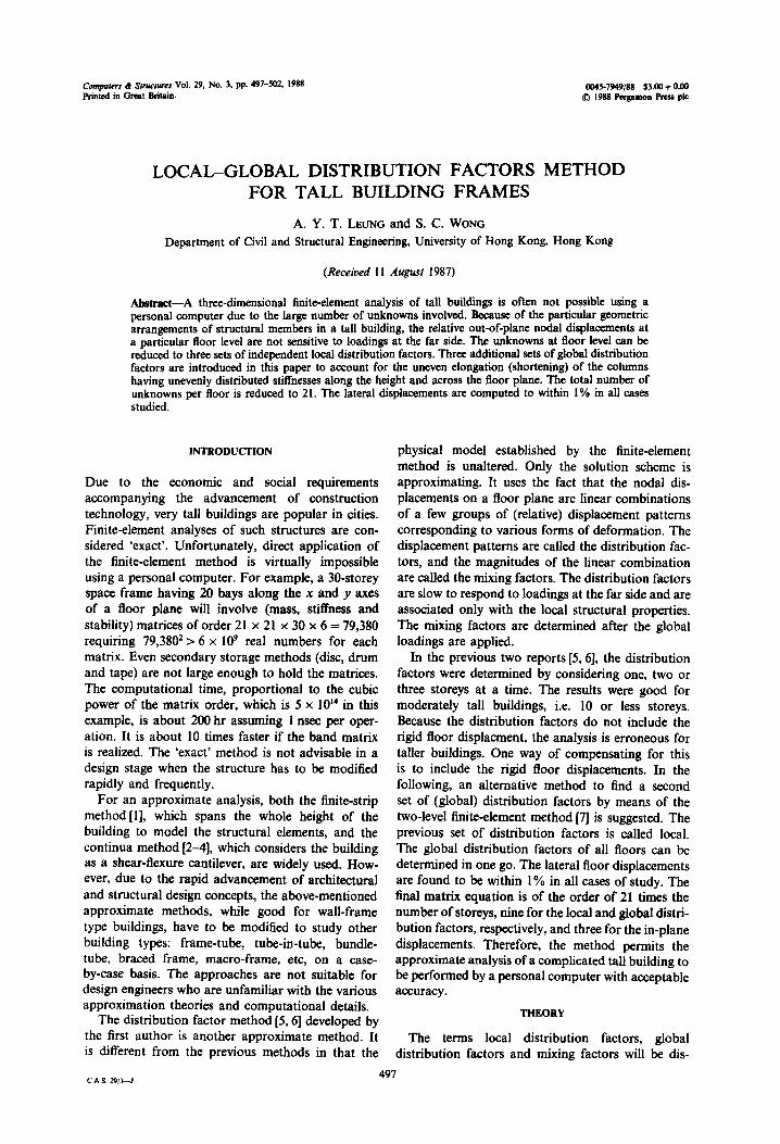
The local distribution factors are obtained by a one-storey model as shown in Fig. 1 and mentioned in [S, S]. In the method, one considers the stiffness associated with floor i,

[K”]{S’} = (F’i. (5)

In partitioned form, according to in-plane and out-of-plane displacements,

where {Fo} includes out-of-plane dead and live loads. We need three sets of displacement patterns for the out-of-plane displa~ments corresponding to unit in-plane displacements {a’, P’, 0’ 1, one at a time; therefore, collectively,

where [I] is a 3 x 3 identity matrix, [R;] IS an unknown reaction matrix to give unit in-plane displa~ments; [Ro] = row (Fo f ; and upon solving eqn (6), vo] consists of the local distribution Factors,

The matrix &Jo] can be determined by the second term of eqn (6),

or, if (Fo) is zero, and hence [Ro] is zero,

Fig. I. A one-storey model.

Local-global distribution factors method for tall building frames 499

deformation:

[L’] =

WII W2I

%I a21

Ill Al

WI2 w22

aI2 a22

812 . B 32

wm i w,i

ad a,i

Ad Bd

w31

a31

81

w32

a32

B 32

W3nl

a3d

83d,

(9)

GLOBAL DISTRIBUTION FACTORS

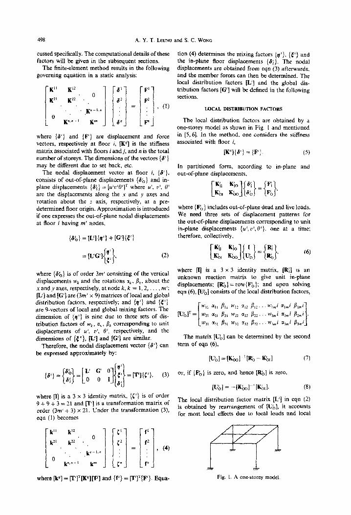
While the local distribution factors are superior in representing local deformation, they are incapable of modelling the out-of-plane deformation of floors far away from the ground due mainly to the uneven extension of the columns along the height. One method of compensating for this is to include the three rigid-body out-of-plane movements as global distribution factors. However, as the columns elongate (shorten) unevenly along the height, the rigid-body movements are not suitable to deal with very tall buildings having abrupt changes of stiffness. An alternative method is to adopt the two-level finite-element method [I which predicts the global behaviour of frames.

In essence, the nodal displacements {8} of a few purposely selected master floors (Fig. 2) of eqn (1) are chosen so that

(8) = col(fi, 6, j, Ii, 1, e>, (10)

where

{*} = col{~,;“}, (1) = col{o?i”), {j} = col{/T~}

{ii} = col{P}, {T} = col{a”), (8) = col{P);

j=l,2,..., is number of nodes at floor m; and m = 1,2,. . . , is number of master floors. The dis- placement vector in eqn (1) is rearranged so that

{S} = col{w, a, i, u, v, e>, (11)

where

{w} = col{w;}, {a} = col{ai}, {/I} = col{&}

{u} = col{l(‘}, {v} = col{o’}, {e} = coqe’};

j=l,2,..., is number of nodes at floor i (i =

1,2,. . . , n). One can choose a suitable interpolating function [N(i)] so that

W; = [N(i)]{*,}, a; = PJ(i)l@,l

pi = [N(i)] {fi}, II’ = [N(i)1 (4

u’ = [N(i)](T), 8’ = PJ(ill{~), (12)

where

{ii,} = co1{~3,“}, {as,} = col{cf~}, (6, = col{jT;);

andm=1,2,..., is number of master floor. If the top floor only is taken as the master floor, then w,, ij, pj, ii, V, 6 are all scalars and N(i) = i/n. It is usual practice to keep the number of master floors to a minimum. If the building stiffness is uniform or changing gradually, the top floor and a middle floor are chosen as masters. For a building having abrupt changes of stiffness at certain floor levels, these floors are taken as masters.

Stove nodas’

fz lntarpdotlng hlnctk+l

\

Fig. 2. A master floors model.

500 A. Y. T. LEUNG and S. C. WONG

According to transfonnation (12), eqn (1) is con- densed to a stiffness equation associated with the

20th floor I x

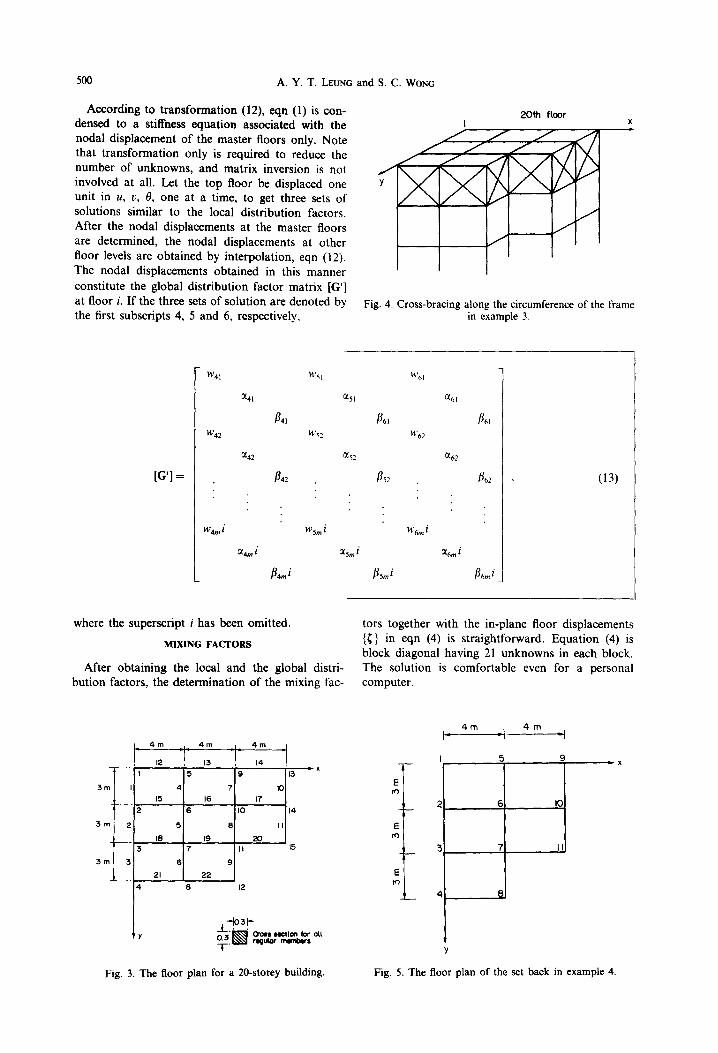
nodal displacement of the master floors only. Note that transformation only is required to reduce the number of unknowns, and matrix inversion is not involved at all. Let the top floor be displaced one unit in u, u, 0, one at a time, to get three sets of solutions similar to the local distribution factors. After the nodal displacements at the master floors are determined, the nodal displacements at other floor levels are obtained by interpolation, eqn (12). The nodal displacements obtained in this manner I I I constitute the global distribution factor matrix [G’] at floor i. If the three sets of solution are denoted by Fig. 4. Cross-bracing along the circumference of the frame the first subscripts 4, 5 and 6, respectively, in example 3.

[G’] = B 42

w,i

_I

where the superscript i has been omitted. tors together with the in-plane floor displacements

MIXING FACI’ORS {{} in eqn (4) is straightforward. Equation (4) is block diagonal having 21 unknowns in each block.

After obtaining the local and the global distri- The solution is comfortable even for a personal bution factors, the determination of the mixing fac- computer.

4m , 4m , 4m I I

12 13 14

5 9 13 x

4 7 IO

I5 I6 I7

6 IO 14

5 8 II

IS IS W 7 II I5

6 9

21 22

4 8 I2

2 6 IO,

3 7 II

4 6_

1 Y

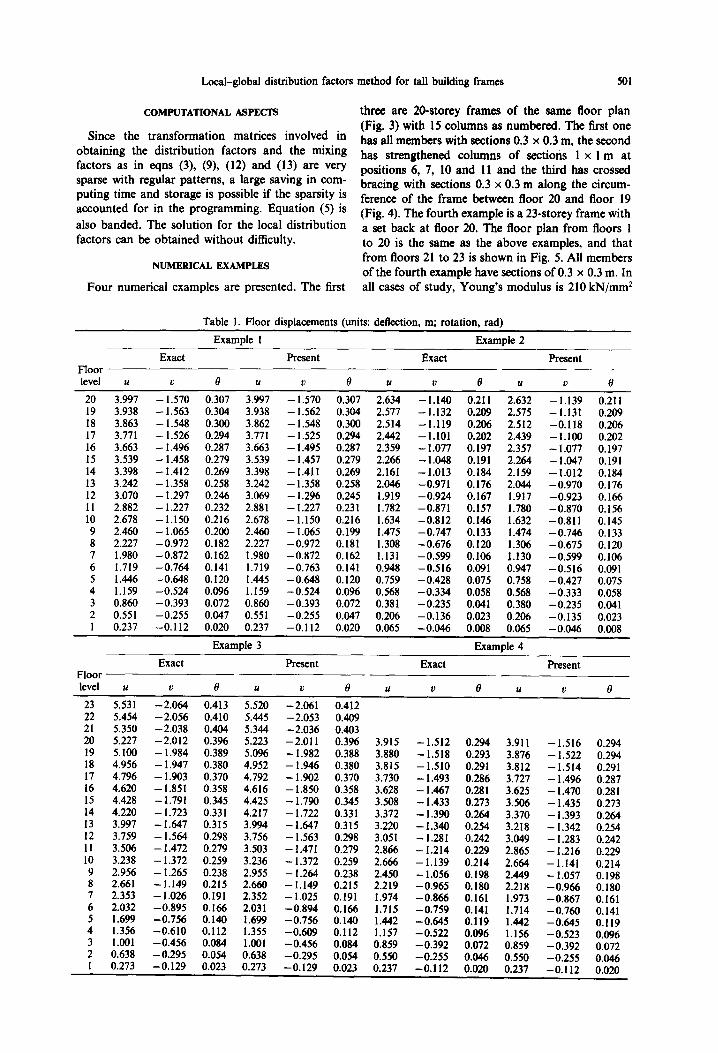
Fig. 3. The floor plan for a 20-storey building. Fig. 5. The floor plan of the set back in example 4.

E m

E ! m

E m

4m , 4m I

I 5 9 cx

Local-global distribution factors method for tall building frames 501

COMPUTATIONAL ASPECI-S

Since the transformation matrices involved in

obtaining the distribution factors and the mixing factors as in eqns (3), (9), (12) and (13) are very sparse with regular patterns, a large saving in com- puting time and storage is possible if the sparsity is accounted for in the programming. Equation (5) is

also banded. The solution for the local distribution factors can be obtained without difficulty.

NUMERICAL EXAMPLES

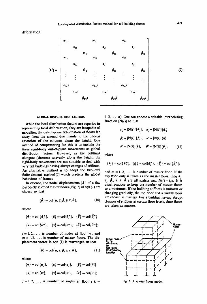
Four numerical examples are presented. The first

three are 20-storey frames of the same floor plan (Fig. 3) with 15 columns as numbered. The first one has all members with sections 0.3 x 0.3 m, the second has strengthened columns of sections 1 x 1 m at positions 6, 7, 10 and 11 and the third has crossed bracing with sections 0.3 x 0.3 m along the circum- ference of the frame between floor 20 and floor 19 (Fig. 4). The fourth example is a 23-storey frame with a set back at floor 20. The floor plan from floors 1 to 20 is the same as the above examples, and that from floors 21 to 23 is shown in Fig. 5. All members of the fourth example have sections of 0.3 x 0.3 m. In all cases of study, Young’s modulus is 210 kN/mm2

Table 1. Floor displacements (units: deflection, m; rotation, rad)

Example I Example 2

Exact Present Exact Present Floor level u V e U V e U V e U V e 20 3.997 -1.570 0.307 3.997 - 1.570 0.307 2.634 -1.140 0.211 2.632 -1.139 0.211 19 3.938 -1.563 0.304 3.938 - 1.562 0.304 2.577 -1.132 0.209 2.575 -1.131 0.209 18 3.863 -1.548 0.300 3.862 -1.548 0.300 2.514 -1.119 0.206 2.512 -0.118 0.206 17 3.771 - 1.526 0.294 3.771 - 1.525 0.294 2.442 -1.101 0.202 2.439 -1.100 0.202 16 3.663 - 1.496 0.287 3.663 -1.495 0.287 2.359 -1.077 0.197 2.357 -1.077 0.197 15 3.539 - 1.458 0.279 3.539 - 1.457 0.279 2.266 -1.048 0.191 2.264 - 1.047 0.191 14 3.398 -1.412 0.269 3.398 -1.411 0.269 2.161 -1.013 0.184 2.159 -1.012 0.184 13 3.242 - 1.358 0.258 3.242 - 1.358 0.258 2.046 -0.971 0.176 2.044 -0.970 0.176 12 3.070 - 1.297 0.246 3.069 - 1.296 0.245 1.919 -0.924 0.167 1.917 -0.923 0.166 11 2.882 -1.227 0.232 2.881 -1.227 0.231 1.782 -0.871 0.157 1.780 -0.870 0.156 10 2.678 -1.150 0.216 2.678 -1.150 0.216 1.634 -0.812 0.146 1.632 -0.811 0.145 9 2.460 - 1.065 0.200 2.460 -1.065 0.199 1.475 -0.747 0.133 1.474 -0.746 0.133 8 2.227 -0.972 0.182 2.227 -0.972 0.181 1.308 -0.676 0.120 1.306 -0.675 0.120 7 1.980 -0.872 0.162 1.980 -0.872 0.162 1.131 -0.599 0.106 1.130 -0.599 0.106 6 1.719 -0.764 0.141 1.719 -0.763 0.141 0.948 -0.516 0.091 0.947 -0.516 0.091 5 1.446 -0.648 0.120 1.445 -0.648 0.120 0.759 -0.428 0.075 0.758 - 0.427 0.075 4 1.159 -0.524 0.096 1.159 -0.524 0.096 0.568 -0.334 0.058 0.568 -0.333 0.058 3 0.860 -0.393 0.072 0.860 -0.393 0.072 0.381 -0.235 0.041 0.380 -0.235 0.041 2 0.551 -0.255 0.047 0.551 -0.255 0.047 0.206 -0.136 0.023 0.206 -0.135 0.023 1 0.237 -0.112 0.020 0.237 -0.112 0.020 0.065 -0.046 0.008 0.065 -0.046 0.008

Example 3 Example 4

Exact Present Exact Present Floor level u V e U V e u V e U V e 23 5.531 -2.064 0.413 5.520 -2.061 0.412 22 5.454 -2.056 0.410 5.445 -2.053 0.409 21 5.350 -2.038 0.404 5.344 - 2.036 0.403 20 5.227 -2.012 0.396 5.223 -2.011 0.396 3.915 -1.512 0.294 3.911 - 1.516 0.294 19 5.100 - 1.984 0.389 5.096 - 1.982 0.388 3.880 -1.518 0.293 3.876 - I .522 0.294 18 4.956 - 1.947 0.380 4.952 -1.946 0.380 3.815 -1.510 0.291 3.812 - 1.514 0.291 17 4.796 -1.903 0.370 4.792 -1.902 0.370 3.730 - 1.493 0.286 3.727 - 1.496 0.287 16 4.620 -1.851 0.358 4.616 -1.850 0.358 3.628 -1.467 0.281 3.625 - 1.470 0.281 15 4.428 - 1.791 0.345 4.425 - 1.790 0.345 3.508 - 1.433 0.273 3.506 - 1.435 0.273 14 4.220 -1.723 0.331 4.217 -1.722 0.331 3.372 - 1.390 0.264 3.370 - 1.393 0.264 13 3.997 -1.647 0.315 3.994 -1.647 0.315 3.220 -1.340 0.254 3.218 - 1.342 0.254 12 3.759 -1.564 0.298 3.756 -1.563 0.298 3.051 - 1.281 0.242 3.049 - 1.283 0.242 11 3.506 -1.472 0.279 3.503 - 1.471 0.279 2.866 -1.214 0.229 2.865 - 1.216 10

0.229 3.238 - 1.372 0.259 3.236 - 1.372 0.259 2.666 -1.139 0.214 2.664

9 - 1.141

2.956 -1.265 0.214

0.238 2.955 - 1.264 0.238 2.450 -1.056 0.198 2.449 - 1.057 8

0.198 2.661 -1.149 0.215 2.660 -1.149 0.215 2.219 -0.965 0.180 2.218

7 -0.966

2.353 0.180

-1.026 0.191 2.352 - 1.025 0.191 1.974 -0.866 0.161 1.973 6

-0.867 2.032

0.161 -0.895 0.166 2.031 -0.894 0.166 1.715 -0.759 0.141 1.714

5 1.699 -0.756 -0.760 0.141

0.140 1.699 -0.756 0.140 1.442 -0.645 0.119 1.442 4 1.356

-0.645 -0.610

0.119 0.112 1.355 -0.609 0.112 1.157 -0.522 0.096 1.156

3 1.001 -0.523

-0.456 0.096

0.084 1.001 -0.456 0.084 0.859 -0.392 0.072 0.859 2 0.638 -0.295

-0.392 0.072 0.054 0.638 -0.295 0.054 0.550 -0.255

I 0.273 0.046 0.550

-0.129 0.023 0.273 -0.255 0.046

-0.129 0.023 0.237 -0.112 0.020 0.237 -0.112 0.020

502 A. Y. T. LHJUNG and S. C. WONG

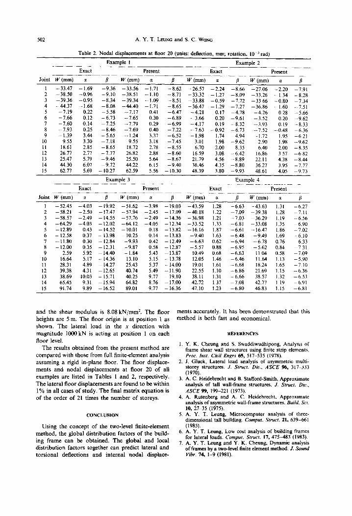
Table 2. Nodal displacements at floor 20 (units: deflection, mm; rotation, LO-’ rad)

Example 1 Example 2 ___

Exact Present Exact Present ~._ _._- Joint W (mm) a B W (mm) a B W (mm) a B W (mm) a B

1 -33.47 -1.69 -9.36 -33.56 -1.71 -8.62 -26.57 -2.24 -8.66 -27.06 -2.20 -7.91 2 -38.50 -0.96 -9.10 -38.51 -1.10 -8.71 -33.32 -1.27 -8.09 -33.26 -1.34 -8.28 3 -39.36 -0.95 -8.34 -39.34 -1.09 -8.51 -33.88 -0.59 -7.72 -33 66 -0.80 -7.34 4 -44.37 - 1.68 -8.08 -44.40 -1.71 -8.65 -36.47 -1.29 -7.27 -36.86 -1.60 -7.51 5 -7.19 0.22 -5.58 -7.17 0.41 -6.47 -4.21 0.17 -4.78 -4.26 0 28 -5.66 6 -7.66 0.12 -6.73 -7.65 0.30 -6.89 -3.66 0.20 -9.61 -3.52 0.20 -9.62 7 -7.60 0.14 -7.25 -7.79 0.29 -6.99 -4.17 0.19 -8.32 -3.93 0.19 -8.33 8 -7.93 0.25 -8.46 -7.69 0.40 -7.22 -7.63 -0.92 -6.73 -7.52 -0.48 -6.36 9 -1.39 3.44 - 5.65 - 1.24 3.37 -6.52 - 1.98 1.74 -4.94 - 1.72 I .95 -621

10 9.55 3.30 -7.18 9.55 3.18 -7.45 3.01 1.98 -9.62 2.90 1.98 -9.62 11 18.61 2.85 -8.65 18.72 2.78 -8.55 6.70 2.00 -8.35 6.40 2.00 -8.35 12 26.77 2.77 -7.77 26.82 2.88 -8.60 16.59 3.08 -6.42 16.86 357 -682 13 25.47 5.79 -9.46 25.50 5.64 -8.67 21.79 4.56 -8.89 22.11 4.38 -8.44 14 44.30 6.07 -9.72 44.22 6.15 -9.40 36.46 4.35 -8.80 36.27 3.95 -7.77 15 62.77 5.69 - 10.27 62.59 5.56 - 10.30 48.39 3.80 -9.93 48.61 4.05 -9.73

Example 3 Example 4 . ..__--._ Exact Present Exact Present ___.__. __.~~________ __

Joint W (mm) a P W (mm) a B W (mm) a P W(mm) a s

1 -52.45 -4.03 - 19.92 -51.62 -3.98 -19.03 -43.59 1.28 -6.63 -43.63 1.31 -6.27 2 -58.21 -2.50 - 17.47 -57.94 -2.45 -17.09 -40.18 1.22 -7.09 -39.38 1.28 -7.11 3 -58.57 -2.49 -14.55 -57.76 -2.49 - 14.36 -36.98 1.21 -7.03 - 36.29 1.19 -6.56 4 -64.29 -4.03 -12.02 -64.12 -4.05 -12.34 -33.52 1.33 -6.81 - 33.08 1.35 -6.90 5 - 12.89 0.43 - 14.52 - 10.01 0.18 - 13.82 -16.16 1.87 -6.61 - 16.47 1.86 -7.02 6 - 12.58 0.37 - 13.98 - 10.25 0.14 - 13.83 -9.40 1.63 - 6.48 -9.49 1.69 -6.10 7 -11.80 0.30 - 12.84 -9.93 0.42 - 12.49 -6.63 0.62 -6.94 -6.78 0.76 6.33 8 - 12.00 0.35 - 12.31 - 9.87 0.58 - 12.87 -5.57 0.88 -6.95 - 5.62 0.84 -7 31 9 2.59 5.92 - 14.40 - 1.84 5.43 - 13.87 10.49 0.68 -6.63 II 04 0.58 -7.09

10 16.64 5.17 - 14.36 13.10 5.15 - 13.78 12.05 1.46 - 6.46 11.64 1.13 - 5.90 11 28.31 4.89 - 14.27 25.43 5.37 - 14.00 19.01 1.61 -6.68 18.24 1.65 -7.10 12 39.38 4.31 - 12.65 40.74 5.49 - I 1.90 22.55 1.10 -6.86 21.69 1.15 -6.36 13 38.69 10.03 - 15.71 40.25 9.77 - 19.10 38.11 1.31 -6.66 38.57 1.32 -6.53 14 65.45 9.31 - 15.94 64.82 8.76 -17.00 42.72 1 37 -7.08 42.77 I 19 -6.91 15 91.74 9.89 - 16.52 89.01 9.77 - 16.36 47.10 1.23 -6.80 46.83 1.15 -6.81

and the shear modulus is 8.08 kN/mmZ. The floor heights are 5 m. The floor origin is at position 1 as shown. The lateral load in the x direction with magnitude 1000 kN is acting at position 1 on each floor level.

The results obtained from the present method are compared with those from full finite-element analysis assuming a rigid in-plane floor. The floor displace- ments and nodal displacements at floor 20 of all examples are listed in Tables 1 and 2, respectively. The lateral floor displacements are found to be within 1% in all cases of study. The final matrix equation is of the order of 21 times the number of storeys.

CONCLUSION 5.

Using the concept of the two-level finite-element method, the global distribution factors of the build- ing frame can be obtained. The global and local distribution factors together can predict lateral and torsional deflections and internal nodal displace-

6.

7.

ments accurately. It has been demonstrated that this method is both fast and economical.

1.

2.

3.

4.

REFERENCES

Y. K. Cheung and S. Swaddiwudhipong, Analysts of frame shear wall structures using finite strip elements. Proc. Inst. Civil Engrs 66, 517-535 (1978). J. Gluck, Lateral load analysis of asymmetric multi- storey structures. J. Siruct. Div., AXE 96, 317-333 (1970). A. C. Heidebrecht and B. Stafford-Smith, Approximate analysis of tall wall-frame structures. J. Struct. Div., AXE 99, 199-221 (1973). A. Rutenberg and A. C. Heidebrecht, Approxtmate analysis of asymmetric wall-frame structures. Build. Scl. 10, 27-35 (1975). A. Y. T. Leung, Microcomputer analysis of three- dimensional tall building. Compur. Strut. 21, 639-661 (1985). A. Y. T. Leung, Low cost analysis of building frames for lateral loads. Comput. Struct. 17, 475-483 (1983). A. Y. T. Leung and Y. K. Cheung, Dynamic analysis of frames by a two-level finite element method. J. Sound Vibr. 74, l-9 (1981).