Local Housing Market Cycle and Loss Given Default: Evidence from Sub-Prime

Residential Mortgages

Yanan Zhang, Lu Ji, and Fei Liu

WP/10/167

© 2010 International Monetary Fund WP/10/167 IMF Working Paper Research Department

Local Housing Market Cycle and Loss Given Default: Evidence from Sub-Prime Residential Mortgages

Prepared by Yanan Zhang, Lu Ji, and Fei Liu

Authorized for distribution by Atish Ghosh

July 2010

Abstract

This paper studies the impact of housing market cycles on loss given default (LGD).

Previous studies have shown that the current loan-to-value ratio (CLTV) is the most important determinant of LGD. This paper establishes another linkage which is between the house price cycles before the time of mortgage origination and LGD. The empirical analysis is based on a large loan-level sub-prime residential mortgage loss dataset from 1998 to 2009. Results show that house price history has a long memory in explaining LGD. Its explanatory power far exceeds the original LTV and other loan characteristics. This paper offers a countercyclical view of LGD risk. The model can be combined with a default probability model to serve as a regulatory prudential tool. Such a tool provides a solution to the inherent procyclical bias in BASEL II capital requirements, and can contribute to the safety and soundness of banking institutions.

This Working Paper should not be reported as representing the views of the IMF. The views expressed in this Working Paper are those of the author(s) and do not necessarily represent those of the IMF or IMF policy. Working Papers describe research in progress by the author(s) and are published to elicit comments and to further debate.

JEL Classification Numbers: G21, G28 Keywords: loss given default, residential mortgage, housing market cycle, Basel II, recovery,

loss severity

Author’s E-Mail Address: fliu@imf.org

2

Table of Contents I. Introduction ........................................................................................................................... 3 

II. Data ...................................................................................................................................... 6 

A. Borrowers Characteristics ................................................................................................ 6 

B. Property Characteristics ................................................................................................... 6 

C. Loan Characteristics ......................................................................................................... 7 

D. Housing Market Cycle Information ................................................................................. 8 

E. Geographical Differences in LGD .................................................................................. 10 

III. Empirical Study ................................................................................................................ 12 

A. Model ............................................................................................................................. 12 

B. Results ............................................................................................................................ 14 

C. A summary by determinant categories ........................................................................... 14 

D. Variable-by-variable results ........................................................................................... 15 

E. The effect of the housing market cycle .......................................................................... 17 

IV. Sensitivity Analysis and Robustness Checks ................................................................... 18 

V. Simulation Study and Policy Analysis ............................................................................... 21 

A. Countercyclical prudential tool ...................................................................................... 21 

B. Lukewarm House Price Scenario ................................................................................... 22 

C. Big Boom Scenario ........................................................................................................ 22 

D. Big Bust Scenario........................................................................................................... 22 

E. Up & Down Cycle Scenario ........................................................................................... 22 

F. Down & Up Cycle Scenario ........................................................................................... 23 

G. Summary of All Scenarios ............................................................................................. 23 

VI. Conclusion ........................................................................................................................ 25 

VII. Appendix ......................................................................................................................... 27 

References ............................................................................................................................... 28 

3

I. INTRODUCTION

On November 1, 2007, the Office of the Comptroller of the Currency (OCC) approved a final rule implementing the advanced approaches of the Basel II Capital Accord.1 This new rule allows banks, through the Advanced Internal Ratings Based Approach (A-IRB), to calculate their minimum regulatory capital. Under A-IRB, banks could use their own quantitative models to estimate PD (probability of default), EAD (Exposure at Default), LGD (Loss Given Default) and other parameters required for calculating RWA (Risk Weighted Assets). Then total required capital is calculated as a fixed percentage of the estimated RWA. There have been many studies on PD. The research on LGD, however, remains more limited in the literature. This paper focuses on the LGD component of the A-IRB under Basel II. In particular, we provide a model of LGD that includes the impact of the housing market cycle. Previous studies have shown that the current loan-to-value (CLTV) is the single most important determinant of LGD.2 However, to determine LGD at the time of loan origination for risk-based pricing and capital allocation, only information available at the time of origination is known. Knowing that the CLTV is driven by the historical house price change, we investigate the linkage between house price cycles before mortgage origination and LGD. The new Basel accord has stimulated a growing body of literature on LGD. For example, Schuermann (2004) analyzes the definition and measurement of LGD in the context of Basel II. He also analyzes with data from Moody’s Default Risk Service Database. He finds that the recovery distribution is bimodal, with recoveries lower in recessions than in expansions. His analyses are based on corporate bond data. Altman, Resti and Sironi (2003) conduct a comprehensive review of the literature and the empirical evidence of default recovery rates in credit-risk modeling. Their paper particularly studies the relationship between PD and LGD and how this relationship is treated in different modeling frameworks. The summarized recent empirical evidence suggests that the LGD is positively correlated with PD.3 The aforementioned papers have been focused on wholesale exposures such as corporate bonds and loans. Few studies have been devoted to retail exposure such as residential mortgages and retail credit cards, for two reasons. First, the public data is not readily available. Second, PD modeling has been the primary focus of credit-risk modeling of consumer loans in banks and hence has drawn more attention from researchers. Among the 1 Details of the announcement can be found on the website of OCC via the link http://www.occ.gov/ftp/release/2007-123.htm.

2 See Qi and Yang (2007)

3 See details of the empirical evidence in Frye (2000a, b), Jarrow (2001), Carey and Gordy (2003), and Altman, and others, (2001, 2004).

4

limited literature that studies LGD at retail level, most have focused on testing theories about LGD and various factors that affect LGD. Lekkas, and others, (1993) test the frictionless options-based mortgage default theory empirically. They find that higher loss severity of residential mortgages is associated with higher original LTV, geographical location with higher default and younger mortgage loans. They also find that loss severity is not affected by the difference between the note rate and current interest rates. Their findings do not agree with the propositions on loss severity derived from the frictionless options-based mortgage default theory. Crawford and Rosenblatt (1995) further introduce transactions costs into the options-based mortgage default model and empirically test its effect on loss severity. In recent studies, Pennington-Cross (2003) and Calem and LaCour-Little (2004) have also analyzed the determinants of LGD. Their regression results confirm Lekkas, and others, (1993) in that either original LTV or CLTV; and mortgage age and loan size have significant effects on LGD. More recently, Qi and Yang (2007) study LGD of high LTV loans. They find that CLTV is the single most important determinant of LGD. More interestingly, they create and include an economic downturn dummy in their regression. They find that mortgage loss severity in distressed housing markets is significantly higher than under normal housing market conditions. Bellotti and Crook (2009) study LGD models for UK retail credit cards. They compare several econometric methods for modeling LGD and find that Ordinary Least Squares models with macroeconomic variables perform best to forecast LGD at both the account level and the portfolio level. The inclusion of macroeconomic variables enables them to model LGD in downturn conditions as required by Basel II. Most of these studies have focused on testing theories and determinants. Studies on business cycle effects remain limited. There have been some attempts to test the downturn effect. For example, Calem (2003) studies the relationship between LGD and economic downturn based on simulation at the portfolio level. Qi and Yang (2007) test housing market downturns through a dummy variable. Otherwise, there is a lack of studies of the relationship between the housing market cycle and LGD in the literature. A growing body of literature studies the procyclical tendency of BASEL II. Some even blame BASEL II capital requirements for exacerbating the credit bubble and worsening the financial crisis. Saurina (2006) studies credit cycles and documents why actual credit risk increases during the credit expansion period while bank risk-measurement models and capital requirements imply that actual credit risk decreases. He proposes a counter-cyclical loan-loss reserve model as a solution. Griffith-Jones (2009) argues for “leaning against the wind” when it comes to financial regulation. He calls for inclusion of counter-cyclical elements in the BASEL Capital Accord to mitigate the inherent pro-cyclicality of the IRB approach. Gordy (2004) discusses various ways to introduce counter-cyclical methods to dampen the procyclical impact of the IRB approach. The three methods he discussed are: through-the-

5

cycle risk measurement, flattening the PD function and smoothing out the PD function. All three methods are indirect approaches and minor adjustments to the existing framework; none offered a systematic solution to the procyclical problem. In this paper, we estimated a LGD model that has built-in counter-cyclical LGD views by incorporating local housing cycles. If combined with an appropriate PD model, it can offer a systematic solution to the procyclical problem. In the present paper, we present an empirical study on a large loan-level sub-prime residential mortgage loss dataset from 1998 to 2009. In our study, controlling for original LTV and other loan characteristics that are used in most previous studies, we test the relation between the housing market cycle and LGD. To check the robustness of our results, we conducted several sensitivity and robustness analyses based on various business cycle periods and geographical regions. These reinforce our basic model results. Furthermore, using our estimates of the underlying structural relationships, we analyzed LGD in different house price scenarios through simulations. We find that the historical housing market cycle has a significant impact on LGD. Our simulations show that our model provides a countercyclical prudential tool that can be used in compliance with Basel II capital requirements. The present paper contributes to the existing literature on LGD in the following ways. First, we studied the effect of the housing market cycle in a systematic way. Second, our LGD model has countercyclical views, which offers a direct and systematic solution to the procyclical BASEL capital requirement problem. Third, most regression models that use information at mortgage origination (such as OLTV) suffer from poor model fit (with R2 ranging from 0.02 to 0.14).4 We provide a way to improve the R-square to about 0.20. Lastly, our data cover the most recent housing market cycle and financial crisis in the U.S. Hence we offer insights to housing policy makers from integrating the recent boom and bust experience in our study. This paper is organized as follows. We describe our data and carry out several data analyses in Section 2. In Section 3, we present our model formally and discuss the results. We carry out sensitivity analysis and robustness checks in Section 4. In Section 5, we simulate different housing market cycle scenarios and provide policy insights from a countercyclical capital management perspective. We conclude in Section 6.

4 See Qi and Yang (2007) for a model survey.

6

II. Data

Our data is from Loan Performance asset-backed securities (ABS) database. It is nationally representative covering the entire country. It includes loans originated from 1998 to 2008, with loss information up to December 2009. The wide geographical coverage and the long performance history that encompasses a full boom-and-bust cycle are very useful for our study. Our database has 838,683 residential mortgage loans. The average original balance is $218,558 and the average loss rate (LGD) is 62 percent. Our study focuses on the average loss rate to understand its determinants and its relationship with housing market cycles. We classify loan data characteristics into three categories, which are borrower, property and loan characteristics, described as follows.

A. Borrowers Characteristics

There are a few borrower-related variables that we believe are important. They are indicators for second liens, cash-out refinance, investor and reduced documentation. The second lien flag indicates whether the borrower has another lien on the same property. Second liens increase the total loan amount collateralized and increase the total LTV, which is associated with high loss severity. In our sample, 0.9 percent of the loans have second liens. Investors refer to borrowers who invest on real estate property for capital gains through house price appreciations. About 15 percent of the mortgages in our sample are investor loans, which are associated with high LGD. In terms of loan purpose, 37 percent are cash-out refinance. These loans in general have higher LGD. Reduced documentation borrowers refer to those with fewer documents than required by standard underwriting procedure and may be associated with greater risk of high LGD. In our sample, about 54 percent of the loans are identified as low documentation.

B. Property Characteristics

Property characteristics describe the collateral type and also may be important to evaluate LGD. Our data consists of 6.8 percent condominiums, 1.3 percent manufactured housing and the rest as single-family. Condos take a small share of the real estate market compared to single-family houses. Condos tend to concentrate in large cities and the price for condos may suffer from greater variations. Condos are smaller in size compared to other single-family homes thus often associated with smaller loans. As discussed below, smaller loans tend to

7

have higher LGD, as do the largest loans. Manufactured housing is relatively larger and therefore associate with higher LGD. In addition, more than 4 percent of the mortgages in our sample are on houses with more than two units. Multiple-unit loans usually have higher LGD than single units.

C. Loan Characteristics

There are a number of important mortgage characteristics that are related to both default risk and loss severity. The most important one is loan-to-value ratio. On average, the LTV at origination in our sample is 82 percent, meaning that borrowers put 18 percent of the house price as a down payment at settlement. High LTV is associated with high default risk. Previous empirical studies (cited above) also found that high LTV at origination is associated with high LGD. More than 40 percent of the mortgages in our sample have LTVs higher than 80 percent. More than 10 percent have LTVs higher than 90 percent. Loan size is another important factor. High loss ratios are often found among small loans, as some fixed or transactional costs that are calculated into loss can become large proportions of the loan amount. On average, the loan size is about $218,000 at origination in our sample. Another factor is the note rate on the loan, as higher note rates are associated with higher LGDs due to increased amount of lost interest in a loss event. There are different loan products ranging from fixed rate to ARM and varying by different years of loan maturity. More than 65 percent of the mortgages in our sample are ARMs. These mortgages turn out to have higher LGD than 30 year fixed. This could be a result of the types of borrowers who elect (or self-select) to take ARMs. Details of product types and their shares in our sample can be found in the summary statistics, Table 1. Variable definitions are in the Appendix.

8

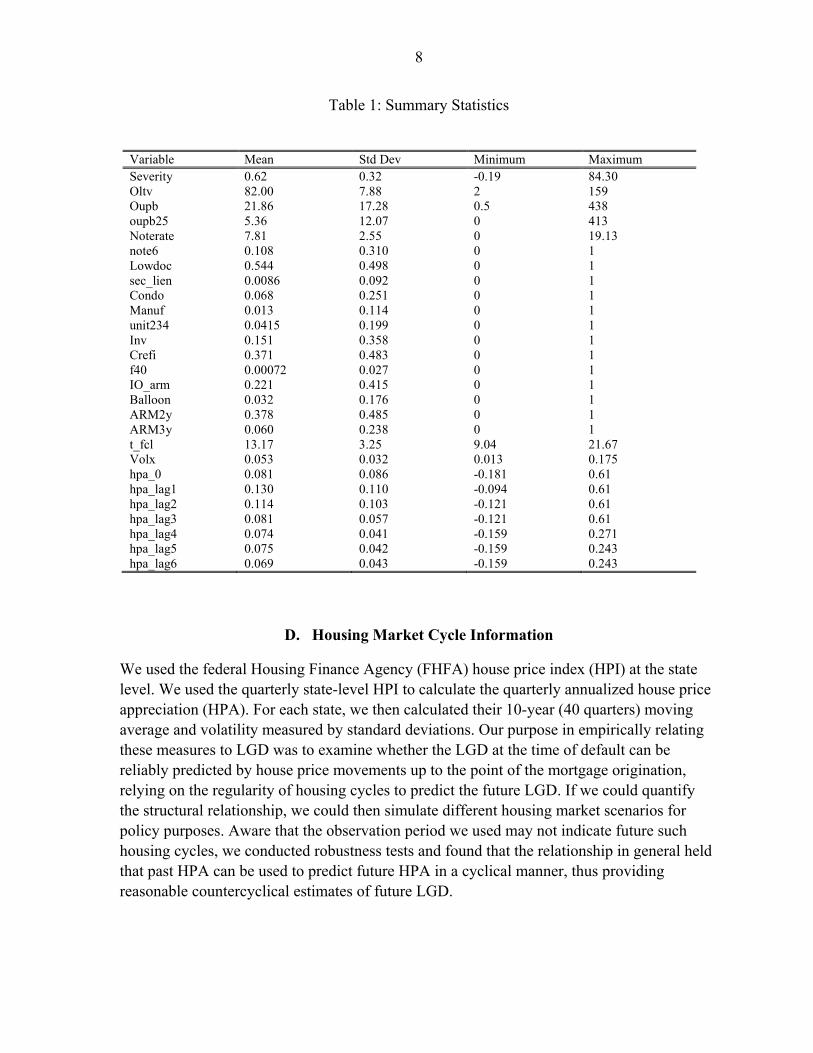
Table 1: Summary Statistics

D. Housing Market Cycle Information

We used the federal Housing Finance Agency (FHFA) house price index (HPI) at the state level. We used the quarterly state-level HPI to calculate the quarterly annualized house price appreciation (HPA). For each state, we then calculated their 10-year (40 quarters) moving average and volatility measured by standard deviations. Our purpose in empirically relating these measures to LGD was to examine whether the LGD at the time of default can be reliably predicted by house price movements up to the point of the mortgage origination, relying on the regularity of housing cycles to predict the future LGD. If we could quantify the structural relationship, we could then simulate different housing market scenarios for policy purposes. Aware that the observation period we used may not indicate future such housing cycles, we conducted robustness tests and found that the relationship in general held that past HPA can be used to predict future HPA in a cyclical manner, thus providing reasonable countercyclical estimates of future LGD.

Variable Mean Std Dev Minimum Maximum Severity 0.62 0.32 -0.19 84.30 Oltv 82.00 7.88 2 159 Oupb 21.86 17.28 0.5 438 oupb25 5.36 12.07 0 413 Noterate 7.81 2.55 0 19.13 note6 0.108 0.310 0 1 Lowdoc 0.544 0.498 0 1 sec_lien 0.0086 0.092 0 1 Condo 0.068 0.251 0 1 Manuf 0.013 0.114 0 1 unit234 0.0415 0.199 0 1 Inv 0.151 0.358 0 1 Crefi 0.371 0.483 0 1 f40 0.00072 0.027 0 1 IO_arm 0.221 0.415 0 1 Balloon 0.032 0.176 0 1 ARM2y 0.378 0.485 0 1 ARM3y 0.060 0.238 0 1 t_fcl 13.17 3.25 9.04 21.67 Volx 0.053 0.032 0.013 0.175 hpa_0 0.081 0.086 -0.181 0.61 hpa_lag1 0.130 0.110 -0.094 0.61 hpa_lag2 0.114 0.103 -0.121 0.61 hpa_lag3 0.081 0.057 -0.121 0.61 hpa_lag4 0.074 0.041 -0.159 0.271 hpa_lag5 0.075 0.042 -0.159 0.243 hpa_lag6 0.069 0.043 -0.159 0.243

9

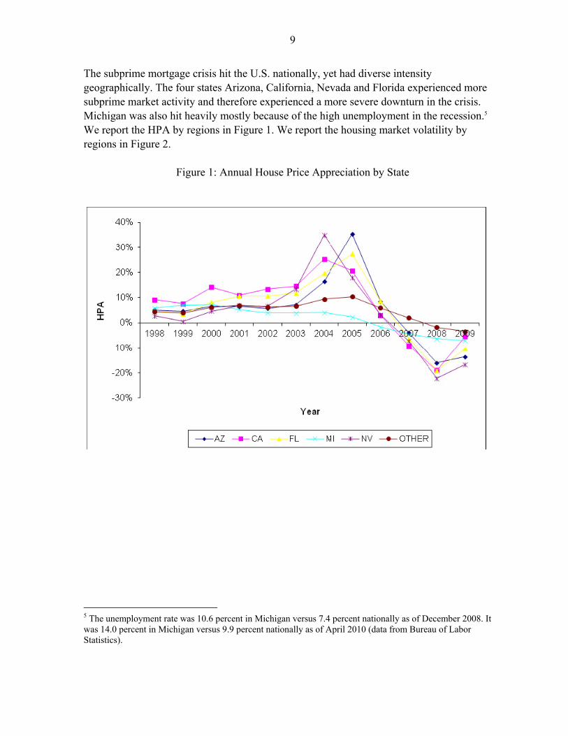
The subprime mortgage crisis hit the U.S. nationally, yet had diverse intensity geographically. The four states Arizona, California, Nevada and Florida experienced more subprime market activity and therefore experienced a more severe downturn in the crisis. Michigan was also hit heavily mostly because of the high unemployment in the recession.5 We report the HPA by regions in Figure 1. We report the housing market volatility by regions in Figure 2.

Figure 1: Annual House Price Appreciation by State

5 The unemployment rate was 10.6 percent in Michigan versus 7.4 percent nationally as of December 2008. It was 14.0 percent in Michigan versus 9.9 percent nationally as of April 2010 (data from Bureau of Labor Statistics).

10

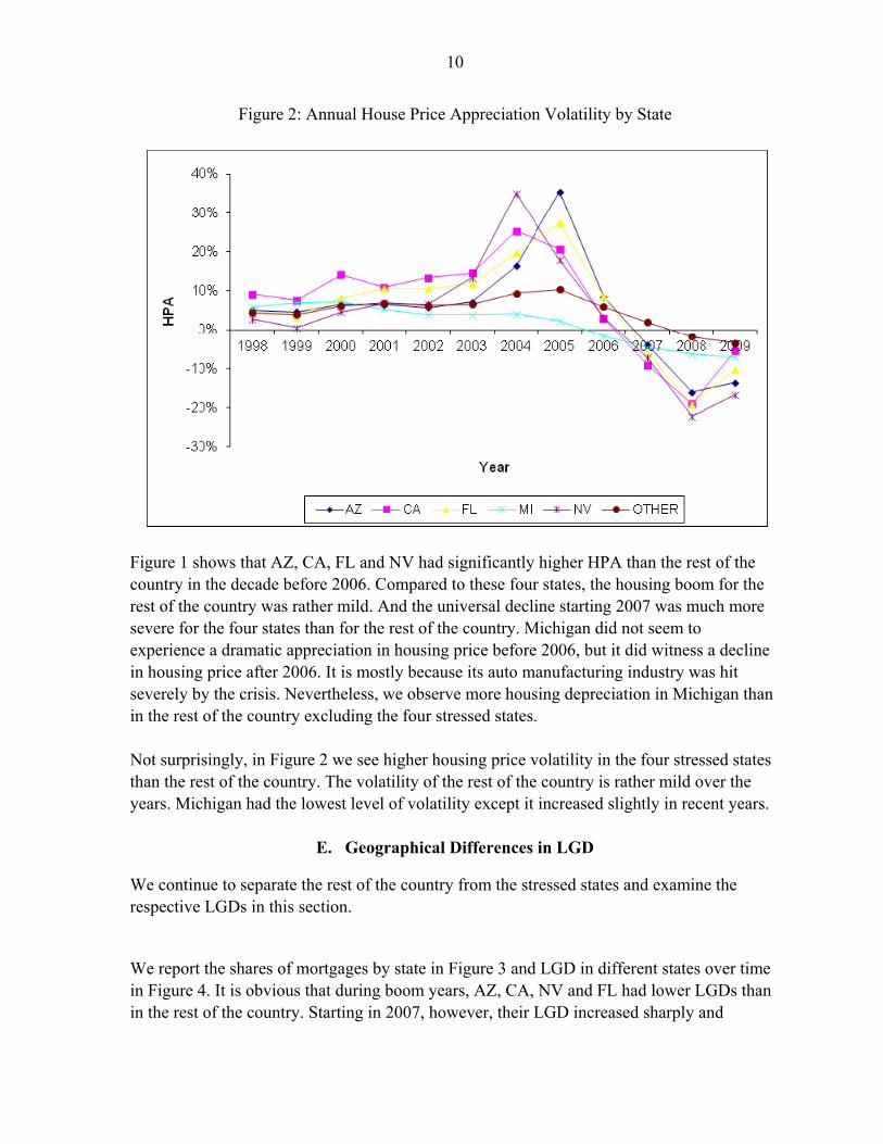
Figure 2: Annual House Price Appreciation Volatility by State

Figure 1 shows that AZ, CA, FL and NV had significantly higher HPA than the rest of the country in the decade before 2006. Compared to these four states, the housing boom for the rest of the country was rather mild. And the universal decline starting 2007 was much more severe for the four states than for the rest of the country. Michigan did not seem to experience a dramatic appreciation in housing price before 2006, but it did witness a decline in housing price after 2006. It is mostly because its auto manufacturing industry was hit severely by the crisis. Nevertheless, we observe more housing depreciation in Michigan than in the rest of the country excluding the four stressed states. Not surprisingly, in Figure 2 we see higher housing price volatility in the four stressed states than the rest of the country. The volatility of the rest of the country is rather mild over the years. Michigan had the lowest level of volatility except it increased slightly in recent years.

E. Geographical Differences in LGD

We continue to separate the rest of the country from the stressed states and examine the respective LGDs in this section.

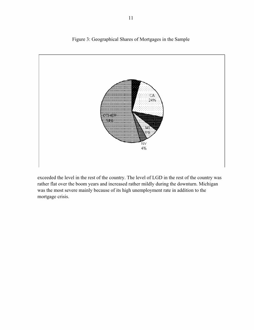
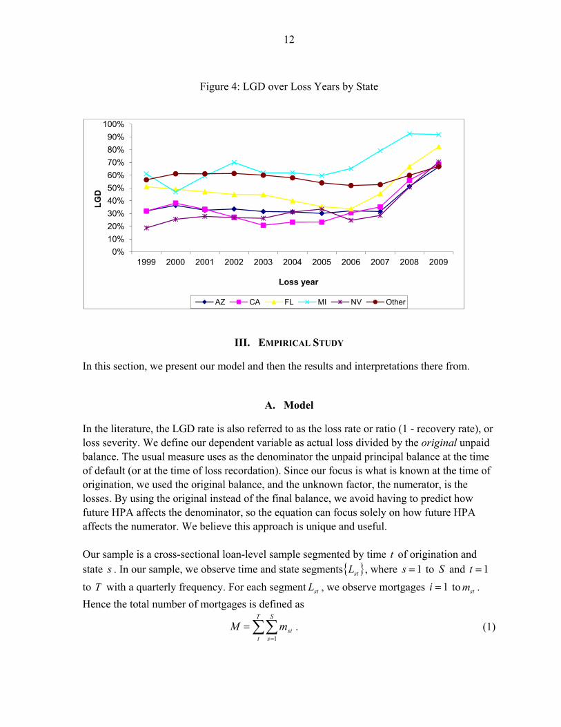
We report the shares of mortgages by state in Figure 3 and LGD in different states over time in Figure 4. It is obvious that during boom years, AZ, CA, NV and FL had lower LGDs than in the rest of the country. Starting in 2007, however, their LGD increased sharply and

 

11

Figure 3: Geographical Shares of Mortgages in the Sample

exceeded the level in the rest of the country. The level of LGD in the rest of the country was rather flat over the boom years and increased rather mildly during the downturn. Michigan was the most severe mainly because of its high unemployment rate in addition to the mortgage crisis.

12

Figure 4: LGD over Loss Years by State

III. EMPIRICAL STUDY

In this section, we present our model and then the results and interpretations there from.

A. Model

In the literature, the LGD rate is also referred to as the loss rate or ratio (1 - recovery rate), or loss severity. We define our dependent variable as actual loss divided by the original unpaid balance. The usual measure uses as the denominator the unpaid principal balance at the time of default (or at the time of loss recordation). Since our focus is what is known at the time of origination, we used the original balance, and the unknown factor, the numerator, is the losses. By using the original instead of the final balance, we avoid having to predict how future HPA affects the denominator, so the equation can focus solely on how future HPA affects the numerator. We believe this approach is unique and useful. Our sample is a cross-sectional loan-level sample segmented by time t of origination and state s . In our sample, we observe time and state segments stL , where 1s to S and 1t

to T with a quarterly frequency. For each segment stL , we observe mortgages 1i to stm .

Hence the total number of mortgages is defined as

T

t

S

sstmM

1

. (1)

0%

10%

20%

30%

40%

50%

60%

70%

80%

90%

100%

1999 2000 2001 2002 2003 2004 2005 2006 2007 2008 2009

LG

D

Loss year

AZ CA FL MI NV Other

13

For each loan i , we observe loss given default istLGD of loan 1i to M , originated at time t

in state s . We also observe a number of loan characteristics ),...,,( ,,2,1 istLististist xxxX , at the

origination time t in state s . In the subsequent sections, we no longer distinguish borrower, property and mortgage characteristics but rather call them simply loan characteristics. At the state level, we observe the time of foreclosure stfcl , which is assumed to be time

invariant and calculated as the ongoing prevalent average length (the number of months) of the foreclosure process in each state. Furthermore, for each state s , at quarter t , we observe the annualized price appreciation sthpa . It is defined and calculated as

1)/( 41, tsstst hpihpihpa . (2)

In addition, we observe the house price volatility over the 10 years prior to time t . It is defined and calculated as

39/)( 239

0,

ksktsst hpahpavol , (3)

where

39

0, 40/

kktss hpahpa (4)

is the 10-year average of HPA prior to time t .

Our model is

istststsistist lagshpaBhpavoltfclXBLGD _54321 , (5)

where lagshpa_ denote lags of HPA for years prior to time t , X is a matrix of variables

other than those based on HPA and foreclosure times, the Bs are vectors of coefficients, the βs are coefficients and ε is the usual error term. (The definitions of the variables are summarized in the Appendix.) We used six lags of HPA after conducting preliminary tests, for two reasons. First, we believe that the historical HPA should have some lag effects that may project the future course of HPA, assuming the existence and some regularity of cycles. Second, we do not want to choose too many lags to over-fit the model. We use HPA and lags of HPA to represent the historical housing market cycle. There are two types of HPA effects. The immediate or current housing price appreciation increases the equity of the property, thereby providing some cushion for future value depreciation. In the short term, the current HPA may reduce LGD. We call this the short-term relief effect. In the literature to date, this has been the only affect included in the analysis of LGD. Long-term

14

lags of HPA show historical value changes. If HPA cycles are endemic and expected to continue, positive HPA over a long term may increase LGD. We call this the long-term penalization effect. The volatility is used to examine how housing market fluctuations affect the LGD. The implication from the volatility is two-fold. On one hand, more volatility means more risk. We label this the risk effect. By intuition we expect more LGD driven by this effect. On the other hand, more volatility means more housing market activity. The market is constantly adjusting its supply and demand equilibrium to satisfy market clearance. We should expect lower LGD if the market is more active. We call this the activity effect. The total effect will be determined by the combination of the two effects. If the risk effect dominates, we will observe a positive effect of the volatility on LGD. It is the other way around if the activity effect dominates.

B. Results

We used ordinary least squares to estimate our model. The adjusted R-square is 0.197 for the entire sample. This is a good fit since this model is based on OLTV and only information available at time of origination. Typically in the literature the R-square would be around 0.1 (see Qi and Yang (2007)) for a model based on OLTV. The following is a summary of the predictive power of the model factors by category of determinants. Presentation of the results by model variables follows.

C. A summary by determinant categories

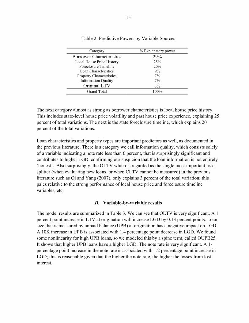
Table 2 summarizes the predictive power of our LGD model by variable category. We see borrower characteristics as the most important set of determinants of LGD. This includes whether the borrower has a second lien, is an investor, and and/or takes out cash with the mortgage loan. One important result here is that second liens are strong predictors of LGD.

15

Table 2: Predictive Powers by Variable Sources

The next category almost as strong as borrower characteristics is local house price history. This includes state-level house price volatility and past house price experience, explaining 25 percent of total variations. The next is the state foreclosure timeline, which explains 20 percent of the total variations. Loan characteristics and property types are important predictors as well, as documented in the previous literature. There is a category we call information quality, which consists solely of a variable indicating a note rate less than 6 percent, that is surprisingly significant and contributes to higher LGD, confirming our suspicion that the loan information is not entirely ‘honest’. Also surprisingly, the OLTV which is regarded as the single most important risk splitter (when evaluating new loans, or when CLTV cannot be measured) in the previous literature such as Qi and Yang (2007), only explains 3 percent of the total variation; this pales relative to the strong performance of local house price and foreclosure timeline variables, etc.

D. Variable-by-variable results

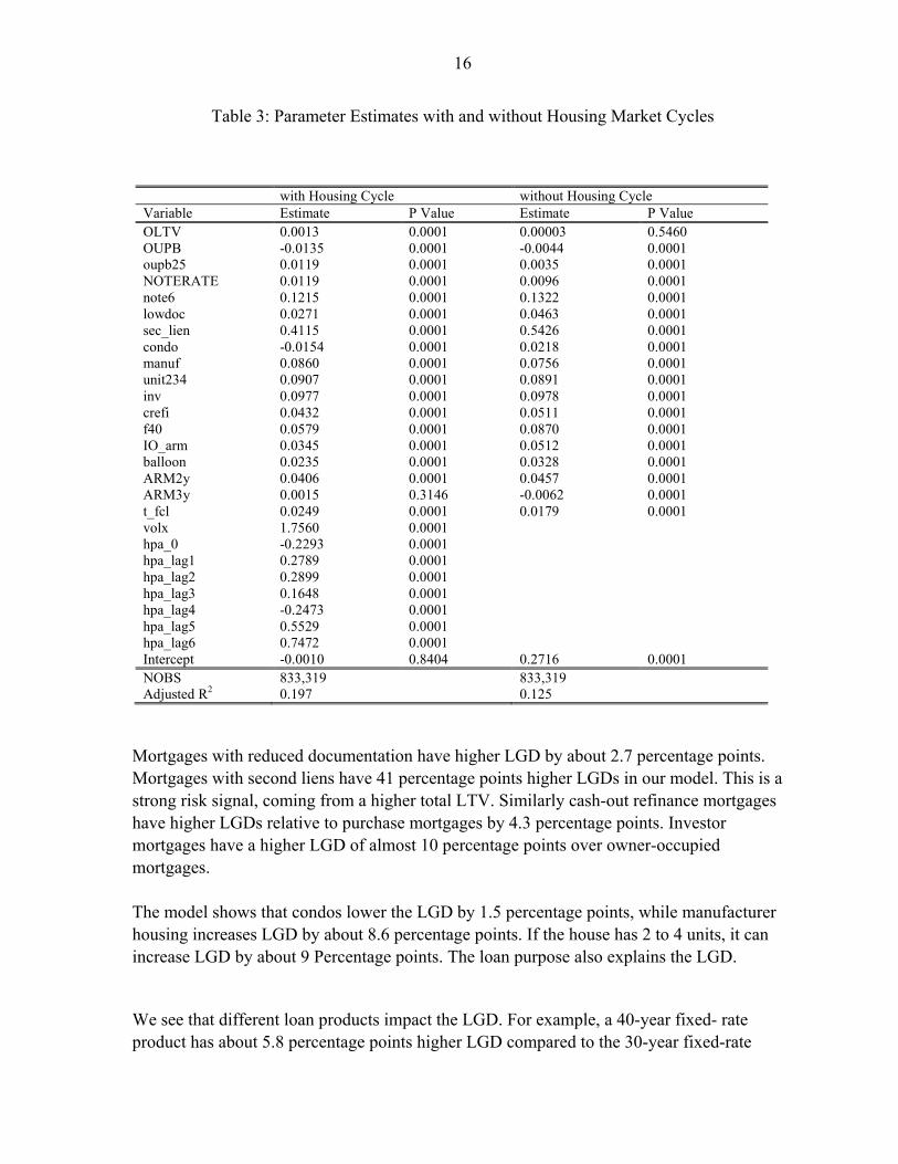
The model results are summarized in Table 3. We can see that OLTV is very significant. A 1 percent point increase in LTV at origination will increase LGD by 0.13 percent points. Loan size that is measured by unpaid balance (UPB) at origination has a negative impact on LGD. A 10K increase in UPB is associated with 1.4 percentage point decrease in LGD. We found some nonlinearity for high UPB loans, so we modeled this by a spine term, called OUPB25. It shows that higher UPB loans have a higher LGD. The note rate is very significant. A 1-percentage point increase in the note rate is associated with 1.2 percentage point increase in LGD; this is reasonable given that the higher the note rate, the higher the losses from lost interest.

Category % Explanatory power

Borrower Characteristics 29% Local House Price History 25%

Foreclosure Timeline 20% Loan Characteristics 9%

Property Characteristics 7% Information Quality 7%

Original LTV 3% Grand Total 100%

16

Table 3: Parameter Estimates with and without Housing Market Cycles

Mortgages with reduced documentation have higher LGD by about 2.7 percentage points. Mortgages with second liens have 41 percentage points higher LGDs in our model. This is a strong risk signal, coming from a higher total LTV. Similarly cash-out refinance mortgages have higher LGDs relative to purchase mortgages by 4.3 percentage points. Investor mortgages have a higher LGD of almost 10 percentage points over owner-occupied mortgages. The model shows that condos lower the LGD by 1.5 percentage points, while manufacturer housing increases LGD by about 8.6 percentage points. If the house has 2 to 4 units, it can increase LGD by about 9 Percentage points. The loan purpose also explains the LGD.

We see that different loan products impact the LGD. For example, a 40-year fixed- rate product has about 5.8 percentage points higher LGD compared to the 30-year fixed-rate

with Housing Cycle without Housing Cycle Variable Estimate P Value Estimate P Value OLTV 0.0013 0.0001 0.00003 0.5460 OUPB -0.0135 0.0001 -0.0044 0.0001 oupb25 0.0119 0.0001 0.0035 0.0001 NOTERATE 0.0119 0.0001 0.0096 0.0001 note6 0.1215 0.0001 0.1322 0.0001 lowdoc 0.0271 0.0001 0.0463 0.0001 sec_lien 0.4115 0.0001 0.5426 0.0001 condo -0.0154 0.0001 0.0218 0.0001 manuf 0.0860 0.0001 0.0756 0.0001 unit234 0.0907 0.0001 0.0891 0.0001 inv 0.0977 0.0001 0.0978 0.0001 crefi 0.0432 0.0001 0.0511 0.0001 f40 0.0579 0.0001 0.0870 0.0001 IO_arm 0.0345 0.0001 0.0512 0.0001 balloon 0.0235 0.0001 0.0328 0.0001 ARM2y 0.0406 0.0001 0.0457 0.0001 ARM3y 0.0015 0.3146 -0.0062 0.0001 t_fcl 0.0249 0.0001 0.0179 0.0001 volx 1.7560 0.0001 hpa_0 -0.2293 0.0001 hpa_lag1 0.2789 0.0001 hpa_lag2 0.2899 0.0001 hpa_lag3 0.1648 0.0001 hpa_lag4 -0.2473 0.0001 hpa_lag5 0.5529 0.0001 hpa_lag6 0.7472 0.0001 Intercept -0.0010 0.8404 0.2716 0.0001 NOBS 833,319 833,319 Adjusted R2 0.197 0.125

17

product. Two-year ARMs are associated with 4 percentage points higher LGD compared to 30-year fixed rate. Interest-only ARMs have about 3.5 percentage points higher LGD than 30-year fixed rate. Balloon mortgages are associated with 2.4 percentage points higher LGD. Lastly, foreclosure timeline is a very important determinant of LGD. The foreclosure timeline is affected by state foreclosure laws, and there is considerable variation of timelines among states across the nation (from Table 1, the standard deviation is 3.25 months with the lowest 9.04 months and the highest 21.67 months). One month increase in the foreclosure timing means 2.5 percent more LGD, for the overall sample.

E. The effect of the housing market cycle

We included HPA at the time of origination and 6 lagged values of HPA, each of which is measured as an annual average as shown in equation (2). The current HPA is negatively related to LGD, meaning that house price appreciation immediately prior to loan origination has the effect of reducing LGD in the future. This is reasonable since house price appreciation tends to have positive short-term serial correlation and negative long-term serial correlation, in the nature of cycles. The model results imply that positive HPA will continue in the short run, reducing the size of the loan relative to house value, which leads to lower LGD in the future. The lagged HPAs tend to have mostly positive effects, meaning that the higher the historical house price has appreciated, the higher the expected future LGD will be. Another thing to notice is that the lagged HPA coefficients display a wave pattern: there is a negative coefficient followed by a few positive coefficients. This is consistent with mean-reversion qualities of housing cycles, and also consistent with near-term serial correlation. The HPA volatility during the 10 years before mortgage origination has a positive effect. This means that the more volatile the local housing market, the higher the expected LGD. As a comparative study, we estimated a model without housing cycle information. The model results are in Table 3. The adjusted R square for such a model is 0.125. The housing cycle information improves the model fit by almost 58 percent by boosting the R square to 0.197. The housing cycle information alone accounts for more than 1/3 of the explained variation of LGD in the model. The implication of the housing market cycle information is twofold. First, it suggests that the historical housing market cycle has a long memory. We are able to project its effect far ahead to predict LGD. Second, it means that even without the CLTV, which has been shown to be the single most important determinant of LGD but which is not available at the time of loan origination, we can obtain a good prediction of LGD as early as when mortgages are originated.

18

IV. SENSITIVITY ANALYSIS AND ROBUSTNESS CHECKS

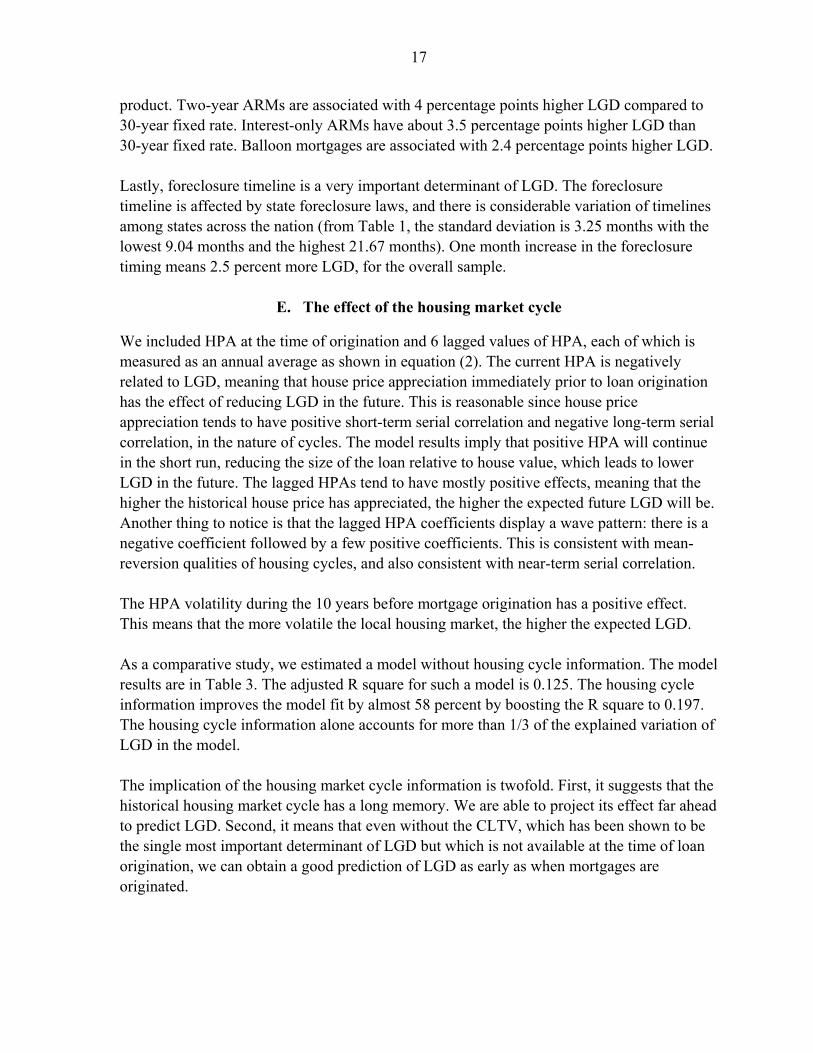
We conduct sensitivity analysis and robustness checks from three different angles. First, we exclude the extremely low and extremely high LGD records, specifically everything below 1 percentile and above 99 percentile from our sample, and replicate the regression. Our purpose is to see whether the results are mostly driven by the extreme observations in the sample. In other words, this would tell us if our findings are still valid without the extreme values in the sample. Second, we exclude several states that experienced most house price declines in the housing crisis, namely Arizona, California, Florida and Nevada. Our intention is to examine the impact, if any, of relatively normal housing cycles. Third, we divide the housing cycle into shorter and selected time periods to examine the impact of housing market cycle. The purpose of conducting this analysis is two-fold. First, it serves a robustness check. We would like to know if the information of the housing market cycle is useful at different points in time of an economic cycle. Second, we also want to understand quantitatively how the LGD responds at different points in the cycle. To this end, we divided our sample into three groups by origination period. Group 1 included mortgages originated between 1998 and 2000, and is featured as a “normal” time. Group 2 included mortgages originated between 2001 and 2006, and is featured as a boom time. Group 3 included mortgages originated between 2007 and 2008, and is featured as downturn (or stressed) time. Table 4 reports the results from the two regressions of the first and second perspectives. The left two columns show the regression results excluding extreme records. The right two columns give the results of the non-stressed states.

19

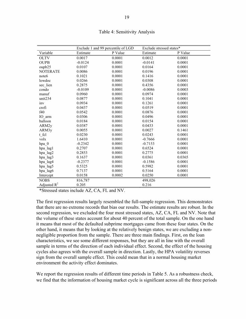
Table 4: Sensitivity Analysis

The first regression results largely resembled the full-sample regression. This demonstrates that there are no extreme records that bias our results. The estimate results are robust. In the second regression, we excluded the four most stressed states, AZ, CA, FL and NV. Note that the volume of these states account for about 40 percent of the total sample. On the one hand it means that most of the defaulted subprime mortgages came from these four states. On the other hand, it means that by looking at the relatively benign states, we are excluding a non-negligible proportion from the sample. There are three main findings. First, on the loan characteristics, we see some different responses, but they are all in line with the overall sample in terms of the direction of each individual effect. Second, the effect of the housing cycles also agrees with the overall sample in direction. Lastly, the HPA volatility reverses sign from the overall sample effect. This could mean that in a normal housing market environment the activity effect dominates. We report the regression results of different time periods in Table 5. As a robustness check, we find that the information of housing market cycle is significant across all the three periods

Exclude 1 and 99 percentile of LGD Exclude stressed states* Variable Estimate P Value Estimate P Value OLTV 0.0017 0.0001 0.0012 0.0001 OUPB -0.0124 0.0001 -0.0141 0.0001 oupb25 0.0107 0.0001 0.0164 0.0001 NOTERATE 0.0086 0.0001 0.0196 0.0001 note6 0.1021 0.0001 0.1416 0.0001 lowdoc 0.0266 0.0001 0.0308 0.0001 sec_lien 0.2875 0.0001 0.4356 0.0001 condo -0.0109 0.0001 -0.0086 0.0003 manuf 0.0960 0.0001 0.0974 0.0001 unit234 0.0877 0.0001 0.1041 0.0001 inv 0.0934 0.0001 0.1261 0.0001 crefi 0.0437 0.0001 0.0519 0.0001 f40 0.0542 0.0001 0.0876 0.0001 IO_arm 0.0306 0.0001 0.0496 0.0001 balloon 0.0184 0.0001 0.0154 0.0001 ARM2y 0.0387 0.0001 0.0433 0.0001 ARM3y 0.0055 0.0001 0.0027 0.1461 t_fcl 0.0230 0.0001 0.0243 0.0001 volx 1.6410 0.0001 -0.7666 0.0001 hpa_0 -0.2342 0.0001 -0.7153 0.0001 hpa_lag1 0.2707 0.0001 0.6524 0.0001 hpa_lag2 0.2853 0.0001 0.2775 0.0001 hpa_lag3 0.1637 0.0001 0.0361 0.0365 hpa_lag4 -0.2377 0.0001 -0.1586 0.0001 hpa_lag5 0.5325 0.0001 0.5982 0.0001 hpa_lag6 0.7137 0.0001 0.5164 0.0001 Intercept 0.0158 0.0002 0.0250 0.0001 NOBS 816,787 498,026 Adjusted R2 0.205 0.216

*Stressed states include AZ, CA, FL and NV.

20

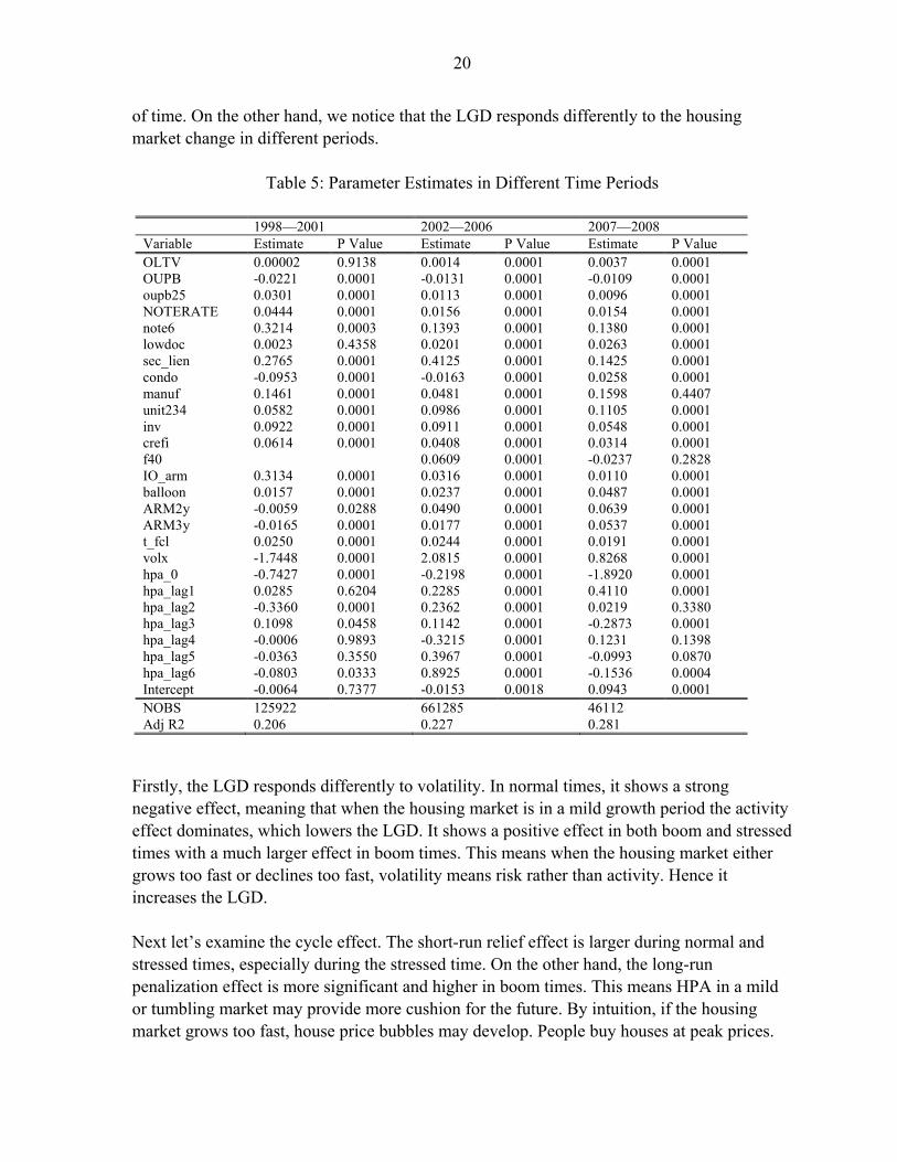
of time. On the other hand, we notice that the LGD responds differently to the housing market change in different periods.

Table 5: Parameter Estimates in Different Time Periods

Firstly, the LGD responds differently to volatility. In normal times, it shows a strong negative effect, meaning that when the housing market is in a mild growth period the activity effect dominates, which lowers the LGD. It shows a positive effect in both boom and stressed times with a much larger effect in boom times. This means when the housing market either grows too fast or declines too fast, volatility means risk rather than activity. Hence it increases the LGD. Next let’s examine the cycle effect. The short-run relief effect is larger during normal and stressed times, especially during the stressed time. On the other hand, the long-run penalization effect is more significant and higher in boom times. This means HPA in a mild or tumbling market may provide more cushion for the future. By intuition, if the housing market grows too fast, house price bubbles may develop. People buy houses at peak prices.

1998—2001 2002—2006 2007—2008 Variable Estimate P Value Estimate P Value Estimate P Value OLTV 0.00002 0.9138 0.0014 0.0001 0.0037 0.0001 OUPB -0.0221 0.0001 -0.0131 0.0001 -0.0109 0.0001 oupb25 0.0301 0.0001 0.0113 0.0001 0.0096 0.0001 NOTERATE 0.0444 0.0001 0.0156 0.0001 0.0154 0.0001 note6 0.3214 0.0003 0.1393 0.0001 0.1380 0.0001 lowdoc 0.0023 0.4358 0.0201 0.0001 0.0263 0.0001 sec_lien 0.2765 0.0001 0.4125 0.0001 0.1425 0.0001 condo -0.0953 0.0001 -0.0163 0.0001 0.0258 0.0001 manuf 0.1461 0.0001 0.0481 0.0001 0.1598 0.4407 unit234 0.0582 0.0001 0.0986 0.0001 0.1105 0.0001 inv 0.0922 0.0001 0.0911 0.0001 0.0548 0.0001 crefi 0.0614 0.0001 0.0408 0.0001 0.0314 0.0001 f40 0.0609 0.0001 -0.0237 0.2828 IO_arm 0.3134 0.0001 0.0316 0.0001 0.0110 0.0001 balloon 0.0157 0.0001 0.0237 0.0001 0.0487 0.0001 ARM2y -0.0059 0.0288 0.0490 0.0001 0.0639 0.0001 ARM3y -0.0165 0.0001 0.0177 0.0001 0.0537 0.0001 t_fcl 0.0250 0.0001 0.0244 0.0001 0.0191 0.0001 volx -1.7448 0.0001 2.0815 0.0001 0.8268 0.0001 hpa_0 -0.7427 0.0001 -0.2198 0.0001 -1.8920 0.0001 hpa_lag1 0.0285 0.6204 0.2285 0.0001 0.4110 0.0001 hpa_lag2 -0.3360 0.0001 0.2362 0.0001 0.0219 0.3380 hpa_lag3 0.1098 0.0458 0.1142 0.0001 -0.2873 0.0001 hpa_lag4 -0.0006 0.9893 -0.3215 0.0001 0.1231 0.1398 hpa_lag5 -0.0363 0.3550 0.3967 0.0001 -0.0993 0.0870 hpa_lag6 -0.0803 0.0333 0.8925 0.0001 -0.1536 0.0004 Intercept -0.0064 0.7377 -0.0153 0.0018 0.0943 0.0001 NOBS 125922 661285 46112 Adj R2 0.206 0.227 0.281

21

In the long run, the market may either slow down or adjust reversely. In other words, the equity generated by the current HPA may not be sustainable. In contrast, in a flat time or in a downturn, people get houses at low prices. The likelihood that the price will go up in the long run is high. Therefore it may continue to generate more equity in the property in the long run. This explains the different patterns we see at different points in the cycle and for different cyclical intensities.

V. SIMULATION STUDY AND POLICY ANALYSIS

In this section we carry out simulation analysis to study the effects of different housing cycles and their policy implications. We demonstrated that our model can serve as a countercyclical prudential tool providing sound countercyclical risk signals.

A. Countercyclical prudential tool

Our model has very high R-square compared to all LGD models using OLTV instead of CLTV. A problem with using CLTV is that we assume to know the exact time of loan default and the corresponding house price growth from origination to the time of default. A model built on CLTV and loan age is obviously not very useful at the time of purchase to evaluate PD or LGD, nor is it useful to help with capital allocation once the loan is in the portfolio. The value of our model is that it can be used to segment risk at the time of origination, and it can be used for allocating capital under the BASEL advanced IRB framework. Not only that, the most important contribution of our model is that it provides a countercyclical view of LGD, as warranted. It overcomes one of the most important shortcomings of the BASEL II advanced IRB framework, which is the procyclical tendency of BASEL II capital requirements. This has been subject to considerable criticism from bankers, policy makers, and researchers. The procyclical capital requirements ignore risk in boom periods that reinforce the euphoria, and the deepening recessions and the credit crunch typically experienced in the bust period. The following simulation exercises demonstrate the predictions of our LGD model in different housing scenarios (Table 6). We use our primary model results, not the models described in the robustness tests, although in practice we recommend that practitioners use the appropriate model for the appropriate type of environment.

22

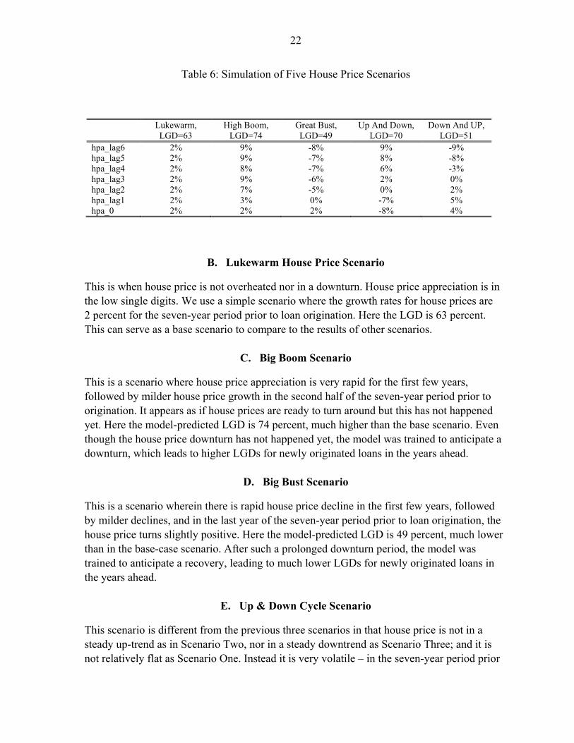
Table 6: Simulation of Five House Price Scenarios

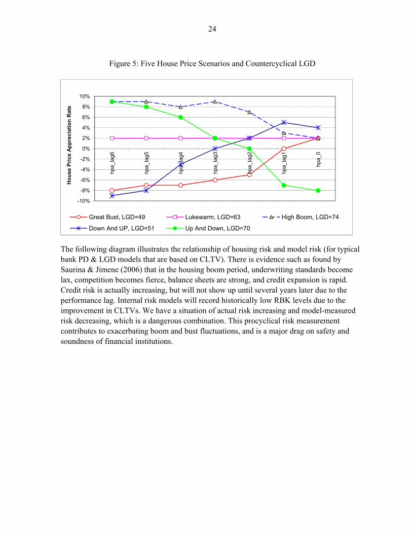
B. Lukewarm House Price Scenario

This is when house price is not overheated nor in a downturn. House price appreciation is in the low single digits. We use a simple scenario where the growth rates for house prices are 2 percent for the seven-year period prior to loan origination. Here the LGD is 63 percent. This can serve as a base scenario to compare to the results of other scenarios.

C. Big Boom Scenario

This is a scenario where house price appreciation is very rapid for the first few years, followed by milder house price growth in the second half of the seven-year period prior to origination. It appears as if house prices are ready to turn around but this has not happened yet. Here the model-predicted LGD is 74 percent, much higher than the base scenario. Even though the house price downturn has not happened yet, the model was trained to anticipate a downturn, which leads to higher LGDs for newly originated loans in the years ahead.

D. Big Bust Scenario

This is a scenario wherein there is rapid house price decline in the first few years, followed by milder declines, and in the last year of the seven-year period prior to loan origination, the house price turns slightly positive. Here the model-predicted LGD is 49 percent, much lower than in the base-case scenario. After such a prolonged downturn period, the model was trained to anticipate a recovery, leading to much lower LGDs for newly originated loans in the years ahead.

E. Up & Down Cycle Scenario

This scenario is different from the previous three scenarios in that house price is not in a steady up-trend as in Scenario Two, nor in a steady downtrend as Scenario Three; and it is not relatively flat as Scenario One. Instead it is very volatile – in the seven-year period prior

Lukewarm, LGD=63

High Boom, LGD=74

Great Bust, LGD=49

Up And Down, LGD=70

Down And UP, LGD=51

hpa_lag6 2% 9% -8% 9% -9% hpa_lag5 2% 9% -7% 8% -8% hpa_lag4 2% 8% -7% 6% -3% hpa_lag3 2% 9% -6% 2% 0% hpa_lag2 2% 7% -5% 0% 2% hpa_lag1 2% 3% 0% -7% 5% hpa_0 2% 2% 2% -8% 4%

23

to loan origination, it is first in a major up-trend then suddenly reverses into a downtrend. How does our model perform in this scenario? The predicted LGD is 70 percent, higher than the base scenario but lower than the ‘Big Boom’s scenario. The predicted LGD is relatively high still because the downtrend had just started and is fairly strong; if it is milder and is well into its course for several years, the predicted LGD will be lower based on our model parameters. We think such a prediction is very reasonable.

F. Down & Up Cycle Scenario

This is a scenario where house price experienced a big downturn in the first few years, then stabilized, followed by a few years of steady house price appreciation. Here the model-predicted LGD is 51 percent, much lower than the base-case scenario. The model anticipates that after the downturn, the house price recovery will continue so that newly originated loans will have lower-than-average LGD. We again think this model prediction is very plausible.

G. Summary of All Scenarios

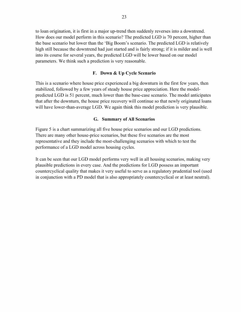
Figure 5 is a chart summarizing all five house price scenarios and our LGD predictions. There are many other house-price scenarios, but these five scenarios are the most representative and they include the most-challenging scenarios with which to test the performance of a LGD model across housing cycles. It can be seen that our LGD model performs very well in all housing scenarios, making very plausible predictions in every case. And the predictions for LGD possess an important countercyclical quality that makes it very useful to serve as a regulatory prudential tool (used in conjunction with a PD model that is also appropriately countercyclical or at least neutral).

24

Figure 5: Five House Price Scenarios and Countercyclical LGD

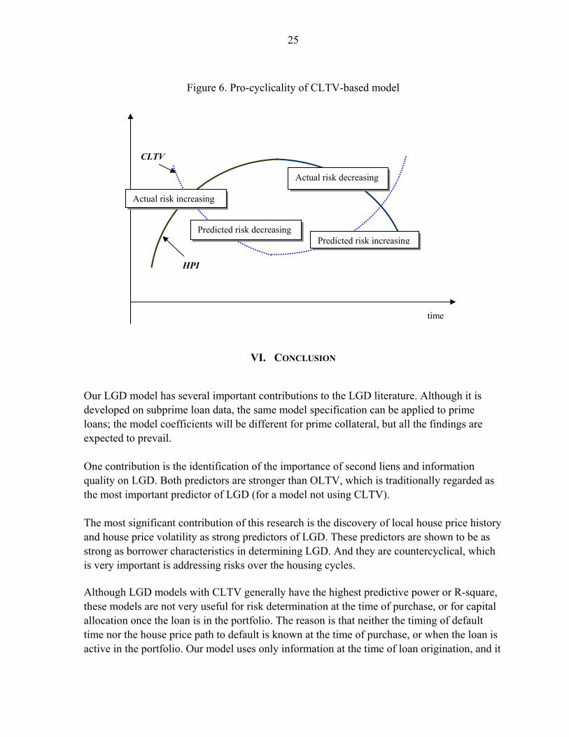
The following diagram illustrates the relationship of housing risk and model risk (for typical bank PD & LGD models that are based on CLTV). There is evidence such as found by Saurina & Jimene (2006) that in the housing boom period, underwriting standards become lax, competition becomes fierce, balance sheets are strong, and credit expansion is rapid. Credit risk is actually increasing, but will not show up until several years later due to the performance lag. Internal risk models will record historically low RBK levels due to the improvement in CLTVs. We have a situation of actual risk increasing and model-measured risk decreasing, which is a dangerous combination. This procyclical risk measurement contributes to exacerbating boom and bust fluctuations, and is a major drag on safety and soundness of financial institutions.

-10%

-8%

-6%

-4%

-2%

0%

2%

4%

6%

8%

10%

hpa_

lag6

hpa_

lag5

hpa_

lag4

hpa_

lag3

hpa_

lag2

hpa_

lag1

hpa_

0

Ho

use

Pri

ce A

pp

reci

ati

on

Rat

e

Great Bust, LGD=49 Lukewarm, LGD=63 High Boom, LGD=74

Down And UP, LGD=51 Up And Down, LGD=70

25

Figure 6. Pro-cyclicality of CLTV-based model

VI. CONCLUSION

Our LGD model has several important contributions to the LGD literature. Although it is developed on subprime loan data, the same model specification can be applied to prime loans; the model coefficients will be different for prime collateral, but all the findings are expected to prevail. One contribution is the identification of the importance of second liens and information quality on LGD. Both predictors are stronger than OLTV, which is traditionally regarded as the most important predictor of LGD (for a model not using CLTV). The most significant contribution of this research is the discovery of local house price history and house price volatility as strong predictors of LGD. These predictors are shown to be as strong as borrower characteristics in determining LGD. And they are countercyclical, which is very important is addressing risks over the housing cycles. Although LGD models with CLTV generally have the highest predictive power or R-square, these models are not very useful for risk determination at the time of purchase, or for capital allocation once the loan is in the portfolio. The reason is that neither the timing of default time nor the house price path to default is known at the time of purchase, or when the loan is active in the portfolio. Our model uses only information at the time of loan origination, and it

Actual risk increasing

Actual risk decreasing

Predicted risk increasing Predicted risk decreasing

CLTV

HPI

time

26

is a very useful tool for risk segmentation at the time of purchase. The R-square of the model is 20 percent, higher than traditional LGD models with OLTV. As a result of including local house price history, our LGD model gives very plausible predictions across all housing cycle scenarios tested (and we have selected the most challenging scenarios to test), leading to the most important implication of our LGD model for capital provision under the advanced BASEL II IRB framework: the model-predicted LGD is countercyclical. Combining with a reasonable (countercyclical) PD model, it should be feasible and useful to develop a prudential tool for capital allocation, one that is countercyclical. The procyclical BASEL capital requirement has been under considerable criticism by bankers, policy makers and researchers alike. We provide a LGD model that can become part of a countercyclical prudential tool to successfully address this very important yet very challenging problem. Such a LGD model can be extended to model seasoned loans (in a separate ongoing research by Ji and Zhang (2010)) and therefore become a set of tools for managing the entire portfolio. With a comprehensive toolkit like this, financial institutions can source new loans and manage seasoned loans with countercyclical risk measurement and capital provision, so the capital buffer will be greater in an expansion period, curtailing the extent of the boom and preparing for future downturns; and the capital cushion will be more forgiving in a recessionary period to dampen the downward drift and actually encourage investments to help promote the recovery. These tools can enhance the safety and soundness of our financial system.

27

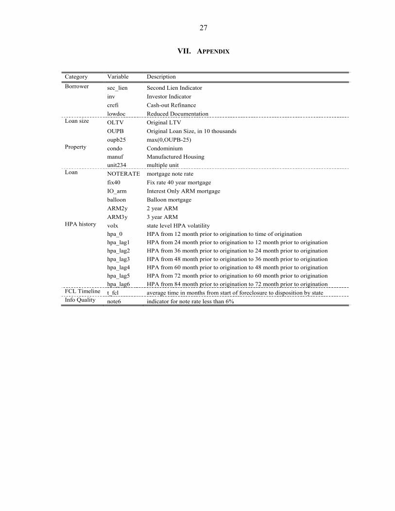
VII. APPENDIX

Category Variable Description

Borrower sec_lien Second Lien Indicator

inv Investor Indicator

crefi Cash-out Refinance

lowdoc Reduced Documentation Loan size OLTV Original LTV

OUPB Original Loan Size, in 10 thousands

oupb25 max(0,OUPB-25) Property condo Condominium

manuf Manufactured Housing

unit234 multiple unit Loan NOTERATE mortgage note rate

fix40 Fix rate 40 year mortgage

IO_arm Interest Only ARM mortgage

balloon Balloon mortgage

ARM2y 2 year ARM

ARM3y 3 year ARM HPA history volx state level HPA volatility

hpa_0 HPA from 12 month prior to origination to time of origination

hpa_lag1 HPA from 24 month prior to origination to 12 month prior to origination

hpa_lag2 HPA from 36 month prior to origination to 24 month prior to origination

hpa_lag3 HPA from 48 month prior to origination to 36 month prior to origination

hpa_lag4 HPA from 60 month prior to origination to 48 month prior to origination

hpa_lag5 HPA from 72 month prior to origination to 60 month prior to origination

hpa_lag6 HPA from 84 month prior to origination to 72 month prior to origination FCL Timeline t_fcl average time in months from start of foreclosure to disposition by state Info Quality note6 indicator for note rate less than 6%

28

REFERENCES

Altman, Edward I., 2001, “Altman High Yield Bond and Default Study,” Salomon

Smith Barney, U.S. Fixed Income High Yield Report, July. Altman, E. and G. Fanjul, 2004, “Defaults and Returns in the High Yield Bond Market:

Analysis Through 2003,” NYU Salomon Center Working Paper, January (also through 2003 Q3).

Altman, Edward, Andrea Resti, and Andrea Sironi, 2003, “Default Recovery Rates In Credit

Risk Modeling: A Review of the Literature and Empirical Evidence,” Working Paper, New York University.

Bellotii, Tony and Jonathan Crook, 2009, “Loss Given Default Models for UK Retail Credit

Cards,” Working Paper, Credit Research Centre, University of Edinburgh Business School.

Calem, Paul S. and Michael LaCour-Little, 2004, “Risk Based Capital Requirements for

Mortgage Loans,” Journal of Banking & Finance, Vol. 28, pp. 647–672. Carey, Mark and Michael Gordy. 2003, “Systematic Risk in Recoveries on Defaulted Debt,”

mimeo, Federal Reserve Board, Washington. Crawford, Fordon W. and Eric Rosenblatt, 1995, “Efficient Mortgage Default Option

Exercise: Evidence from Loss Severity,” The Journal of Real Estate Research, Vol. 10, No.5, pp. 543–555.

Frye, John 2000a, “Collateral Damage”, Risk, April, pp. 91–94. Frye, John 2000b, “Collateral Damage Detected,” Federal Reserve Bank of Chicago,

Working Paper, Emerging Issues Series, October, pp. 1–4. . Gordy, Michael B. and Bradley Howells 2004, “Procyclicality in Basel II: Can We Treat the

Disease Without Killing the Patient?” Grifffith-Jones, Sephany and Jose Ocampo 2009, “Building on the Conter-Cyclical

Consensus: A Policy Agenda. Jarrow, Robert A. 2001, “Default Parameter Estimation Using Market Prices, ”Financial

Analysts Journal, Vol. 57, No. 5, pp. 75–92. Ji, Lu and Yanan Zhang, 2010, “Basel II Loss Given Default Modeling of Seasoned

Residential Mortgage Loans,” Working Paper.

29

Lekkas, Vassilis, John M. Quigley, and Robert Van Order, 1993, “Loan Loss Severity and Optimal Mortgage Default,” Journal of the American Real Estate Research and Urban Economics Association, Vol. 21, No.4, pp. 353–371.

Pennington-Cross, Anthony 2003, “Subprime and Prime Mortgages: Loss Distributions,”

unpublished manuscript, May. Pennington-Cross, Anthony, 2006, “The Duration of Foreclosure in the Subprime Mortgage

Market: A Competing Risks Model with Mixing,” Working Paper, Federal Reserve Bank of St. Louis.

Qi, Min and, Xiaolong Yang, 2007, “Loss Given Default of High Loan-to-Value Residential

Mortgages,” Working Paper, Office of the Comptroller of the Currency. Saurina, Jesus and Gabriel Jimenez, 2006, “Credit Cycles, Credit Risk, and Prudential

Regulation,” International Journal of Central Banking, June 2006. Schuermann, Til, 2004, “What Do We Know About Loss Given Default?” Working Paper,

Wharton Financial Institutions Center.