LOCALIZATION FOR QUASIPERIODIC SCHRODINGER …

LOCALIZATION FOR QUASIPERIODIC SCHRODINGER

OPERATORS WITH MULTIVARIABLE GEVREY

POTENTIAL FUNCTIONS

SILVIUS KLEIN

Abstract. We consider an integer lattice quasiperiodic Schrodinger op-erator. The underlying dynamics is either the skew-shift or the multi-frequency shift by a Diophantine frequency. We assume that the poten-tial function belongs to a Gevrey class on the multi-dimensional torus.Moreover, we assume that the potential function satisfies a generictransversality condition, which we show to imply a Lojasiewicz typeinequality for smooth functions of several variables. Under these as-sumptions and for large coupling constant, we prove that the associatedLyapunov exponent is positive for all energies, and continuous as a func-tion of energy, with a certain modulus of continuity. Moreover, in thelarge coupling constant regime and for an asymptotically large frequency- phase set, we prove that the operator satisfies Anderson localization.

1. Definitions, notations, statement of main results

In this paper we study the one-dimensional lattice quasiperiodic Schrodingeroperator H(x) acting on l2(Z) by:

[H(x)ψ]n := −ψn+1 − ψn−1 + λ v(Tnx)ψn (1.1)

where in equation (1.1):x = (x1, x2) ∈ T2 is a parameter that introduces some randomness into

the system;λ is a real number called the disorder of the system;v(x) is a real valued function on T2 = (R/Z)2, that is, a real valued

1-periodic function in each variable;T is a specific ergodic transformation on T2, and Tn is its nth iteration.

Some of the questions of interest regarding this, or other related oper-ators, are the spectral types (pure point, absolutely continuous, singularlycontinuous), the topological structure of the spectrum, the rate of decay ofthe eigenfunctions, the positivity and regularity of the Lyapunov exponent,the regularity of the integrated density of states.

Due to the ergodicity of the transformation T, the spectrum and thespectral types of the Hamiltonian system [H(x)]x∈T2 defined by (1.1) arenot random - that is, they are independent of x almost surely (see [9]).

1

arX

iv:1

204.

3086

v3 [

mat

h-ph

] 2

9 M

ay 2

013

2 SILVIUS KLEIN

A stronger property than pure point spectrum is Anderson localization,which for the physical model indicates an insulating behavior, while a purelyabsolutely continuous spectrum indicates metallic (conductive) behavior.

Let us describe these concepts more formally.

Definition 1.1. An operator satisfies Anderson localization (AL) if it haspure point spectrum with exponentially decaying eigenfunctions.

Consider now the Schrodinger equation:

H(x)ψ = Eψ (1.2)

for ψ = [ψn]n∈Z ⊂ R and E ∈ R.Due to Schnol-Simon’s theorem (see [9]), to prove AL it is enough to show

that every extended state is exponentially decaying. In other words, if ψ isa formal solution to the Schrodinger equation (1.2) and if ψ grows at most

polynomially∣∣ψn∣∣ . |n| then ψ decays exponentially:

∣∣ψn∣∣ . e−c|n|The Schrodinger equation (1.2) is a second order finite differences equa-

tion:−ψn+1 − ψn−1 + λ v(Tnx)ψn = E ψn

which becomes [ψn+1

ψn

]= MN (x,E)

[ψ1

ψ0

]where

MN (x,E) = MN (x, λ,E) :=

1∏j=N

[λv(Tj x)− E −1

1 0

]is called the transfer (or fundamental) matrix of (1.1).

Define further the function

LN (x,E) = LN (x, λ,E) :=1

Nlog‖MN (x,E)‖

and its mean

LN (E) = LN (λ,E) :=

∫T2

1

Nlog‖MN (x,E)‖ dx

Due to sub-additivity, the sequence LN (E) converges.

Definition 1.2. The limit

L(E) := limN→∞

LN (E)

is called the Lyapunov exponent of (1.1) and it measures the average expo-nential growth of the transfer matrices.

Ergodicity in fact implies that for a.e. x ∈ T2,

L(E) := limN→∞

1

Nlog‖MN (x,E)‖ (1.3)

Note that since the transfer matrices have determinant 1, the Lyapunovexponent is always nonnegative. An important question is whether it is in

SCHRODINGER OPERATORS WITH MULTIVARIABLE GEVREY POTENTIALS 3

fact (uniformly) bounded away from 0. This would imply, due to Kotani’stheorem, absence of absolutely continuous spectrum, and it would representa strong indication for pure point spectrum. This is also usually the as-sumption under which strong continuity properties hold and an analysis ofthe topological structure of the spectrum is more feasible.

In this paper we prove Anderson localization and positivity and continuityof the Lyapunov exponent for large coupling constant, for certain ergodictransformations T on T2 and under certain regularity and transversalityconditions on the potential function v(x). While all of our results are statedand proven for the two-dimensional torus T2, their analogues on the higherdimensional torus hold as well.

We describe the assumptions on the transformation and on the potentialfunction.

We start with some notations: for a multi-index m = (m1,m2) ∈ Z2, wewrite |m| := |m1| + |m2| and if m = (m1,m2) ∈ N2, then m! := m1! ·m2!Moreover, for α = (α1, α2) and m = (m1,m2) ∈ N2, we write α ≤ m whenα1 ≤ m1 and α2 ≤ m2.

Throughout this paper, the transformation T: T2 → T2 will represent:Either the skew-shift

Sω (x1, x2) := (x1 + x2, x2 + ω) (1.4)

where ω ∈ T is irrational.Its nth iteration is given by:

Snω (x1, x2) = (x1 + nx2 +n(n− 1)

2ω, x2 + nω) (1.5)

Or the multi-frequency shift

Tω (x1, x2) := (x1 + ω1, x2 + ω2) (1.6)

where ω = (ω1, ω2) ∈ T2 and ω1, ω2 are rationally independent.Its nth iteration is given by:

Tnω (x) = x+ nω = (x1 + nω1, x2 + nω2) (1.7)

The irrationality / rational independence of the frequency ensures thatthe corresponding transformation is ergodic. However, we need to make aquantitative assumption on this rational independence, for reasons that willbe described later.

We say that the frequency ω ∈ T satisfies a Diophantine condition DCκfor some κ > 0 if

dist (lω,Z) =: ‖l ω‖ > κ · 1

|l| [log(1 + |l|)]2for all l ∈ Z \ 0 (1.8)

4 SILVIUS KLEIN

We say that the (multi)frequency ω ∈ T2 satisfies a Diophantine conditionDCκ for some κ > 0 and a fixed constant A > 2, if

‖l · ω‖ := ‖l1 ω1 + l2 ω2‖ > κ · 1

|l|Afor all l ∈ Z2 \ (0, 0) (1.9)

Note that the set of frequencies which satisfy either (1.8) or (1.9) hasmeasure 1−O(κ), hence almost every frequency satisfies such a Diophantinecondition DCκ for some κ > 0.

When necessary, to emphasize the dependence of the operator on thefrequency, we will use the notation Hω(x) or Hω(x) respectively.

Now we describe the assumptions on the potential function v(x).We say that a C∞ function v(x) on T2 belongs to the Gevrey class

Gs(T2) for some s > 1 if its partial derivatives have the following bounds:

supx∈T2

∣∣∂m v(x)∣∣ ≤MK |m|(m!)s for all m ∈ N2 (1.10)

for some constants M, K > 0.This condition is equivalent (see the exercises from Chapter IV in [15]) to

the following exponential-type decay of the Fourier coefficients of v:∣∣v(l)∣∣ ≤Me−ρ|l|

1/s

for all l ∈ Z2 (1.11)

for some constants M, ρ > 0, where v(x) =∑l∈Z2

v(l) e2πi l·x

Note from (1.10) or (1.11) with s = 1 that the Gevrey class G1(T2) is theclass of real analytic functions on T2.

Note also that s1 < s2 ⇒ Gs1(T2) ⊂ Gs2(T2), so the greater the orderof the Gevrey class, the larger the class.

The Gevrey-class of any order s > 1 is an intermediate Carleman classof functions between analytic functions and C∞ functions. They are not,however, quasi-analytic (one can easily construct examples or use a generaltest for quasi-analyticity of Carleman classes, as in Chapter V.2 in [15]).

We will then impose on our potential function v the following generictransversality condition (TC).

We say that a function v(x) is transversal if v is not flat at any point:

For any x ∈ T2 there is m ∈ N2, |m| 6= 0 such that ∂m v(x) 6= 0 (1.12)

Non-constant analytic functions automatically satisfy (1.12). Therefore,a Schrodinger operator with potential given by a function which satisfies theGevrey regularity condition (1.10) and the transversality condition (1.12) isa natural extension of the non constant analytic case considered in [5], [6].

We are ready to formulate the main result of this paper.

Theorem 1.1. Consider the Schrodinger operator (1.1) on l2(Z):

[H(x)ψ]n := −ψn+1 − ψn−1 + λ v(Tnx)ψn


where the transformation T is either the skew-shift (1.4) or the multi-frequencyshift (1.6). Assume that for some κ > 0 the underlying frequency satisfiesthe Diophantine condition DCκ described in (1.8) or (1.9) respectively.

Assume moreover that the potential function v(x) belongs to a Gevreyclass Gs(T2) and that it is transversal as in (1.12).

There is λ0 = λ0(v, κ) such that the following hold:

If |λ| ≥ λ0, the Lyapunov exponent is positive for all energies E ∈ R:

L(E) ≥ 1

4log |λ| > 0 (1.13)

If |λ| ≥ λ0, the Lyapunov exponent L(E) is a continuous functions ofthe energy E, with modulus of continuity on any compact interval E at least:

h(t) = C e−c|log t|η (1.14)

where C = C(E , λ, v, κ, s) and c, η are some positive absolute constants.

Let T = Sω be the skew-shift. For every λ with |λ| ≥ λ0, there is anexceptional set B = Bλ ⊂ T3, with mesB < κ, such that for all (ω, x) /∈ B,the operator Hω(x) satisfies Anderson localization.

Let T = Tω be the multi-frequency shift. Fix x0 ∈ T2 and λ with|λ| ≥ λ0. Then for a.e. multi-frequency ω ∈ DCκ, the operator Hω(x0)satisfies Anderson localization.

2. Summary of related results, general strategy

The results in this paper extend the ones in [6] and [5] (see also J. Bour-gain’s monograph [4]) from non-constant real analytic potential functions, tothe more general class of Gevrey potential functions satisfying a transversal-ity condition. They also mirror similar results obtained for the one-frequencyshift model on the torus T (see [16]).

It should be noted, however, that unlike the one or multi-frequency shift,the skew-shift, due to its weekly mixing properties, is expected to behavemore like the random model (presumably regardless of the regularity of thepotential). In other words, for the skew-shift, these results are expectedto be independent of the size of the disorder λ. Hence one expects that ifλ 6= 0, the Lyapunov exponent is positive and Anderson localization holdsfor all energies. Moreover, one expects no gaps in the spectrum (unlikein the one-frequency shift case, when the spectrum is a Cantor set) - seethe comments at the end of Chapter 15 in [4]. Some results on these verychallenging problems have been obtained in [2], [3], [18], [19].

Localization results for these types of operators defined by skew-shift dy-namics have applications to quantum chaos problems. More specifically,they imply existence of almost periodic solutions to the quantum kicked ro-tator equation. However, one has to establish (dynamical) localization fora more general, long range operator, one where the discrete Laplacian is re-placed by a Toeplitz operator with fast off-diagonal decay of its monodromy

6 SILVIUS KLEIN

matrix entries. This was already established for analytic potential functions(see Chapter 15 and 16 in [4]), but we will not address this problem forGevrey potential functions in this paper.

Most of the results on localization for discrete quasiperiodic Schrodingeroperators (with either shift or skew-shift dynamics) have been obtained un-der the assumption that the potential function is the cosine function, or atrigonometric polynomial or a real analytic and non-constant function (seeJ. Bourgain’s monograph [4]).

Assuming Gevrey regularity and a transversality condition, there are lo-calization results for the shift model that closely resemble the ones in theanalytic case (see [11], [16]). It should be noted, however, that they areusually perturbative and that more subtle results regarding fine continuityproperties of the integrated density of states (as in [12], [13]) or the topolog-ical structure of the spectrum (as in [14]) are not available in this context.

For potential functions that are more general than Gevrey, namely Cα,the results available now (on localization and positivity of the Lyapunovexponent) require that a(n asymptotically small relative to the size λ ofthe disorder but) positive set of energies be excluded or that the potentialfunction be replaced by some generic variations of itself (see [1], [7], [8]).

To prove Theorem 1.1 we will follow the same strategy used in [16] for thesingle frequency shift model: at each scale, substitute the potential functionby an appropriate polynomial approximation (see Section 3). This in turnwill allow the use of subharmonic functions techniques (see Section 4) devel-oped in [5], [6], [4]. An additional challenge is describing the transversalitycondition (1.12) for multi-variable smooth functions in a quantitive way.We derive (see Section 5) a Lojasiewicz type inequality for such functions,of the kind previously available for non-constant trigonometric polynomials(see [17], [10]) or analytic functions (see [21], [12]).

The main technical result of this paper, from which all statements inTheorem 1.1 follow, is a large deviation theorem (LDT) for logarithmicaverages of transfer matrices (see Section 6).

According to (1.3), due to ergodicity, for a.e. x ∈ T2:

1

Nlog‖MN (x,E)‖ → L(E) as N →∞

The LDT provides a quantitative version of this convergence:

mes [x ∈ T2 :∣∣ 1

Nlog‖MN (x,E)‖ − LN (E)

∣∣ > ε] < δ(N, ε) (2.1)

where ε = o(1) and δ(N, ε)→ 0 as N →∞

The size of the deviation ε and the measure of the exceptional set δ(N, ε)are very important. The sharpest such estimate (see Theorem 7.1 in [12]),available for the single-frequency shift model with analytic potential, holdsfor any ε > 0 and exponentially small measure δ(N, ε) ≈ e−cδN , thus morally


matching the large deviation estimates for random variables that these de-terministic quantities mimic here. Having such sharp estimates leads to asharper modulus of continuity of the Lyapunov exponent (see [12]).

For the multi-frequency shift and the skew-shift models, even with ana-lytic potentials, the available estimates are not as sharp. In this paper, forGevrey potential functions, we will get ε ≈ N−τ and δ ≈ e−N

σfor some

absolute constants τ, σ ∈ (0, 1).

Following the approach in [4], [6], a large deviation estimate like (2.1) willallow us to obtain a lower (positive) bound and continuity of the Lyapunovexponent, once these properties are established at an initial scale N0 forLN0(E). It will also allow us (the reader will be refered to [4], [6] for details)to establish estimates on the Green’s functions associated with the operator(1.1), more specifically the fact that double resonances for Green’s functionsoccur with small probability, which leads to Anderson localization.

Most of the paper will then be devoted to proving a LDT like (2.1):

mes [x ∈ T2 : | 1N

log‖MN (x,E)‖ − LN (E)| > N−τ ] < e−Nσ

(2.2)

through an inductive process on the scale N .

The base step of the inductive process for proving the LDT (2.2) is basedexclusively on the transversality condition (1.12) on the potential, and onchoosing a sufficiently large disorder λ. The latter is what makes this ap-proach perturbative (and, in the case of the skew-shift model, wasteful,since it does not exploit the weakly-mixing properties of its dynamics). Theformer implies a Lojasiewicz type inequality, which we prove using a quan-titative form of the implicit function theorem.

In the inductive step we use the regularity of the potential function v(x)and the arithmetic properties of the frequency. The regularity of v(x) allowsus to approximate it efficiently by trigonometric polynomials vN (x) at eachscale N, and to use these approximants in place of v(x) to get analytic

substitutes MN (x) for the transfer matrices MN (x). Their correspondinglogarithmic averages will be subharmonic in each variable which will allowus to employ the subharmonic functions techniques developed in [4], [5], [6].

The main technical difficulty with this approach, and what restricts it toGevrey (instead of say, Cα) potential functions, is that the holomorphic ex-

tensions of the transfer matrix substitutes MN (x) will have to be restrictedto domains of size ≈ N−δ for some δ > 0. In other words, the estimateswill not be uniform in N , and this decreasing width of the domain of holo-morphicity will have to be overpowered. This will not be possible for a Cα

potential function because its trigonometric polynomial approximation isless efficient, so the width of holomorphicity in this case will decrease toofast (exponentially fast).

8 SILVIUS KLEIN

3. Description of the approximation process

Let v ∈ Gs(T2) be a Gevrey potential function. Then

v(x) =∑l∈Z2

v(l)e2πi l·x (3.1)

where for some constants M,ρ > 0, its Fourier coefficients have the decay:∣∣v(l)∣∣ ≤Me−ρ|l|

1/sfor all l ∈ Z2 (3.2)

We will compare the logarithmic averages of the transfer matrix

LN (x,E) =1

Nlog‖MN (x,E)‖ dx =

1

Nlog‖

1∏j=N

[λv(Tj x)− E −1

1 0

]‖

(3.3)with their means

LN (E) =

∫T2

LN (x,E) dx (3.4)

To be able to use subharmonic functions techniques, we will have to ap-proximate the potential function v(x) by trigonometric polynomials vN (x)and substitute v by vN into (3.3). At each scale N we will have a differentapproximant vN chosen in such a way that the “transfer matrix substitute”would be close to the original transfer matrix. The approximant vN willthen have to differ from v by a very small error - (super)exponentially small

in N . That, in turn, will make the degree deg vN =: N of this polynomialvery large - based on the rate of decay (1.11) of the Fourier coefficients of

v, N should be a power of N , dependent on the Gevrey class s.The trigonometric polynomial vN (x) has an extension vN (z), z = (z1, z2),

which is separately holomorphic on the whole complex plane in each variable.We have to restrict vN (z) in each variable to a narrow strip (or annulus, ifwe identify the torus T with R/Z) of width ρN , where ρN ≈ (deg vN )−1 ≈N−1 ≈ N−θ, for some power θ > 0. This is needed in order to get a uniformin N bound on the extension vN (z). Moreover, in the case of the skew-shift,this is also needed because its dynamics expands in the imaginary direction,and in this case, the width of holomorphicity in the second variable will haveto be smaller than in the first by a factor of ≈ 1

N .The fact that the “substitutes” vN (x) have different, smaller and smaller

widths of holomorphicity creates significant technical problems compared tothe case when v(x) is a real analytic function. It also makes this approachfail when the rate of decay of the Fourier coefficients of the potential functionv(x) is slower.

Therefore, we have to find the optimal “error vs. degree” approximationsof v(x) by trigonometric polynomials vN (x). Here are the formal calcula-tions.


For every positive integer N , consider the truncation

vN (x) :=∑|l|≤N

v(l) e2πi l·x (3.5)

where N = deg vN will be determined later.Since vN (x1, x2) is in each variable a 1-periodic, real analytic function on

R, it can be extended to a separately in each variable 1-periodic holomorphicfunction on C:

vN (z) :=∑|l|≤N

v(l)e2πi l·z (3.6)

To ensure the uniform boundedness in N of vN (z1, z2) we have to restrictvN (z1, z2) to the annulus/strip [|=z| < ρ1,N ]× [|=z| < ρ1,N ], where

ρ1,N :=ρ

2N−1+1/s

Indeed, if z1 = x1 + iy1, z1 = x1 + iy1 and |y1| , |y2| < ρ1,N , then:

∣∣vN (z1, z2)∣∣ =

∣∣∑|l|≤N

v(l)e2πi l·z∣∣ ≤ ∑|l|≤N

∣∣v(l)∣∣e−2π l·y

≤M∑|l|≤N

e−ρ|l|1/se|l1||y1|+|l2||y2| ≤M

∑|l|≤N

e−ρ|l|1/se|l| ρ1,N

≤M∑|l|≤N

e−ρ|l|1/s · e|l| ρ/2 |l|−1+1/s

=M∑|l|≤N

e−ρ2|l|1/s

≤M∑l∈Z2

e−ρ2|l|1/s =:B <∞

where B is a constant which depends on v (not on the scale N) and we have

used : |y1| , |y2| < ρ1,N = ρ2N−1+1/s ≤ ρ

2 |l|−1+1/s for |l| ≤ N , since s > 1.

We also clearly have |v(x)− vN (x)| . e−ρN1/sfor all x ∈ T2.

We will need, as mentioned above, super-exponentially small error inhow vN (x) approximates v(x), otherwise the error would propagate and thetransfer matrix substitutes will not be close to the original transfer matrices.

Hence N should be chosen such that say e−ρN1/s ≤ e−ρN

2. So if N := N2s,

then the width of the holomorphic (in each variable) extension vN (z) will

be ρ1,N = ρ2N

2s(−1+ 1s

) = ρ2N−2(s−1) =: ρ2N

−δ, where δ := 2 (s− 1) > 0.

We conclude: for every integer N ≥ 1, we have a function vN (x) on T2

such that ∣∣v(x)− vN (x)∣∣ < e−ρN

2(3.7)

and vN (x) has a 1-periodic separately holomorphic extension vN (z) to thestrip [|=z| < ρ1,N ]× [|=z| < ρ1,N ], where ρ1,N = ρ

2N−δ, for which∣∣vN (z)

∣∣ ≤ B (3.8)

10 SILVIUS KLEIN

The positive constants ρ, B, δ above depend only on v (not on the scale N).The constant δ depends on the Gevrey class of v: δ := 2(s− 1) so it is fixedbut presumably very large.

We now substitute these approximants vN (x) for v(x) in the definition ofthe transfer matrix MN (x).

Let

A(x,E) :=[λv(x)− E −1

1 0

]be the cocycle that defines the transfer matrix MN (x).

Consider then

AN (x,E) :=[λvN (x)− E −1

1 0

]which leads to the transfer matrix substitutes

MN (x,E) :=

1∏j=N

AN (Tjx,E)

To show that the substitutes are close to the original matrices, we useTrotter’s formula. This is a wasteful approach, and clearly in part responsi-ble for our inability to apply these methods beyond Gevrey functions. Thereare other, much more subtle reasons for why this approach is limited to thisclass of functions.

MN (x)− MN (x) =

=N∑j=1

A(TNx) . . . A(Tj+1x) [A(Tjx)− AN (Tjx)] AN (T j−1x) . . . AN (Tx)

A(Tjx)− AN (Tjx) =

[λv(Tjx)− λvN (Tjx) 0

0 0

]so

‖A(Tjx)− AN (Tjx)‖ ≤ |λ| supy∈T2

∣∣v(y)− vN (y)∣∣ < |λ| e−ρN2

Since supx∈T2 |v(x)| ≤ B, the spectrum of the operator H(x) is containedin the interval [−2 − |λ| B, 2 + |λ| B ]. Hence it is enough to consider onlythe energies E such that |E| ≤ 2 + |λ|B. We then have:

‖A(Tjx)‖ =∥∥∥[ λv(Tjx)− E −1

1 0

]∥∥∥ ≤ |λ| B+∣∣E∣∣+2 ≤ 2 |λ|B+4 ≤ eS(λ)

and

‖AN (Tjx)‖ ≤∥∥∥[ λvN (Tjx)− E −1

1 0

]∥∥∥ ≤ |λ| B +∣∣E∣∣+ 2 ≤ eS(λ)


Therefore,

‖A(Tjx)‖, ‖AN (Tjx)‖ ≤ eS(λ) (3.9)

where S(λ) ≈ log |λ| is a scaling factor that depends only on the (assumedlarge) disorder λ and on v (the constants inherent in ≈ depend on thenumber B = B(v) which also determines the range of spectral values E).

We then have:

‖MN (x,E)− MN (x,E)‖ ≤N∑j=1

eS(λ) . . . eS(λ) |λ| e−ρN2eS(λ) . . . eS(λ) ≤

≤ eNS(λ)−ρN2 ≤ e−ρ2N2

provided N & S(λ).Hence uniformly in x ∈ T2 we get:

‖MN (x,E)− MN (x,E)‖ ≤ e−ρ2N2

(3.10)

provided we chooseN & S(λ) (3.11)

which means roughly that λ has to be at most exponential in the scale N .

We are now going to turn our attention to the logarithmic averages of thetransfer matrices.

Since detMN (x) = 1 and det MN (x) = 1, we have that ‖MN (x)‖ ≥ 1 and

‖MN (x)‖ ≥ 1. Thus, for all N & S(λ) and for every x ∈ T2,

∣∣ 1

Nlog‖MN (x)‖ − 1

Nlog‖MN (x)‖

∣∣ ≤ 1

N‖MN (x)− MN (x)‖ < e−

ρ2N2

Recall the following notation:

LN (x,E) =1

Nlog‖MN (x,E)‖ dx (3.12)

and define its substitute:

uN (x,E) :=1

Nlog ||MN (x)|| (3.13)

Therefore, uniformly in x ∈ T2 and in the energy E:∣∣LN (x,E)− uN (x,E)∣∣ < e−

ρ2N2

and by averaging in x: ∣∣LN (E)− 〈uN (E)〉∣∣ < e−

ρ2N2

where LN (E) :=∫T2 LN (x,E) dx and for any function u(x), 〈u〉 :=

∫T2 u(x) dx.

The advantage of the substitutes uN (x) is that they extend to pluri-subharmonic functions in a neighborhood of the torus T2, as explained be-low.

For the skew-shift transformation T = Sω we consider the strip AρN

:=

[|=z| < ρ1,N ]×[|=z| < ρ2,N ] where ρ1,N = ρ4N−δ and ρ2,N :=

ρ1,N2N = ρ

4N−δ−1

12 SILVIUS KLEIN

We have to reduce the size of the strip in the second variable to accountfor the fact that the skew-shift expands in the imaginary direction. Ourapproximation method required a reduction in the size of the holomorphic-ity strip at each scale, and this additional reduction will be comparativelyharmless.

If we extend the map Sω from T2 = (R/Z)2 to C2, by

Sω(z1, z2) = (z1 + z2, z2 + ω)

we get as in (1.5) that

Snω(z1, z2) = (z1 + nz2 +n(n− 1)

2ω, z2 + nω)

Then if (z1, z2) ∈ AρN

and if we perform n ≤ N iterations, we have:∣∣=(z1 + nz2 +n(n− 1)

2ω)∣∣ =

∣∣=(z1 + nz2)∣∣ = |y1 + ny2| <

ρ

2N−δ (3.14)

The matrix function

AN (x) =[λvN (x)− E −1

1 0

]extends to a 1-periodic, separately in each variable holomorphic matrix val-ued function:

AN (z) :=[λvN (z)− E −1

1 0

]Using (3.8) and the definition of the scaling factor S(λ), we have that on

the strip AρN

the matrix valued function AN (z) is uniformly in N bounded

by eS(λ). Combining this with (3.14), the transfer matrix substitutes extendon the same strip to separately holomorphic matrix valued functions

MN (z, E) :=

1∏j=N

AN (Sjω z, E)

such that, for all z ∈ AρN

and for all energies E we have

‖MN (z, E)‖ ≤ eNS(λ)

Therefore,

uN (z) :=1

Nlog‖MN (z)‖

is a pluri-subharmonic function on the strip AρN

, and for any z in this strip,

|uN (z)| ≤ S(λ)

The same argument applies to the multifrequency shift T = Tω. Theextension of this dynamics to the complex plane

Tω(z1, z2) = (z1 + ω1, z2 + ω2)

does not expand in the imaginary direction, so there is no need to decreasethe width of the strip in the second variable as in the case of the skew-shift.


However, for convenience of notations, we will choose the same strip AρN

for both transformations.We can now summarize all of the above into the following.

Lemma 3.1. For fixed parameters λ,E, for a fixed transformation T = Sωor T = Tω and for δ = 2(s − 1), at every scale N we have a 1-periodicfunction

uN (x) :=1

Nlog‖MN (x)‖

which extends to a pluri-subharmonic function uN (z) on the strip AρN

=

[|=z| < ρ1,N ]× [|=z| < ρ2,N ], where ρ1,N ≈ N−δ, ρ2,N ≈ N−δ−1 so that

|uN (z)| ≤ S(λ) for all z ∈ AρN

(3.15)

Note that the bound (3.15) is uniform in N .Moreover, if N & S(λ), then the logarithmic averages of the transfer

matrices MN (x) are well approximated by their substitutes uN (x):∣∣ 1

Nlog‖MN (x)‖ − uN (x)

∣∣ . e−N2(3.16)∣∣LN − 〈uN 〉∣∣ . e−N2(3.17)

All the inherent constants in the above (and future) estimates are eitheruniversal or depend only on v (and not on the scale N) so they can beignored. The estimates above are independent of the variable x, the param-eters λ,E and the transformation T.

This s a crucial technical result in our paper, which will allow us to usesubharmonic functions techniques as in [4], [6] for the functions uN , and thentransfer the relevant estimates to the rougher functions they substitute.

The logarithmic averages of the transfer matrix have an almost invariance(under the dynamics) property:

Lemma 3.2. For all x ∈ T2, for all parameters λ,E and for all transfor-mations T we have :∣∣ 1


Nlog‖MN (Tx)‖

∣∣ . S(λ)

N(3.18)

Proof. ∣∣ 1


Nlog‖MN (Tx)‖

∣∣ =∣∣ 1

Nlog

‖MN (x)‖‖MN (Tx)‖

∣∣=∣∣ 1

Nlog

‖A(TNx) · . . . ·A(T2x) ·A(Tx)‖‖A(TN+1x) ·A(TNx) · . . . ·A(T2x)‖

∣∣≤ 1

Nlog[ ‖(A(TN+1x))−1‖ · ‖A(Tx)‖ ] .

S(λ)

N

where the last bound is due to (3.9). The inequality (3.18) then follows.

14 SILVIUS KLEIN

4. Averages of shifts of pluri-subharmonic functions

One of the main ingredients in the proof of the LDT (2.2) is an estimateon averages of shifts of pluri-subharmonic functions. These averages areshown to converge in a quantitative way to the mean of the function. Theresult holds for both the skew-shift and the multi-frequency shift.

For the skew-shift, the result was proven in [6] (see Lemma 2.6 there).We will reproduce here the scaled version of that result, the one that takesinto account the size of the domain of subharmonicity and the sup norm ofthe function. The reader can verify, by following the details of the proof in[6], that this is indeed the correct scaled version. For the multi-frequencyshift, the result is essentially contained within the proof of Theorem 5.5 in[4], but for completeness, we will include here the details of its proof.

Proposition 4.1. Let u(x) be a real valued function on T2, that extends to apluri-subharmonic function u(z) on a strip Aρ = [|=z1| < ρ1]× [|=z2| < ρ2].

Let ρ = minρ1, ρ2. Let T be either the skew-shift or the multi-frequencyshift on T2, where the underlying frequency satisfies the DCκ described in(1.8) or (1.9) respectively. Assume that

supz∈Aρ

|u(z)| ≤ S

Then for some explicit constants σ0, τ0 > 0, and for n ≥ n(κ) we have:

mes [x ∈ T2 :∣∣ 1n

n−1∑j=0

u(Tjx) − 〈u〉∣∣ > S

ρn−τ0 ] < e−n

σ0(4.1)

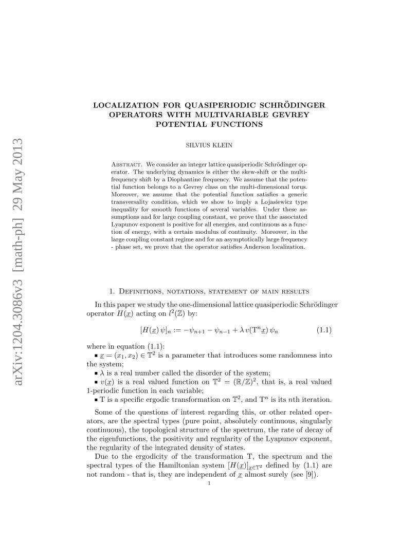
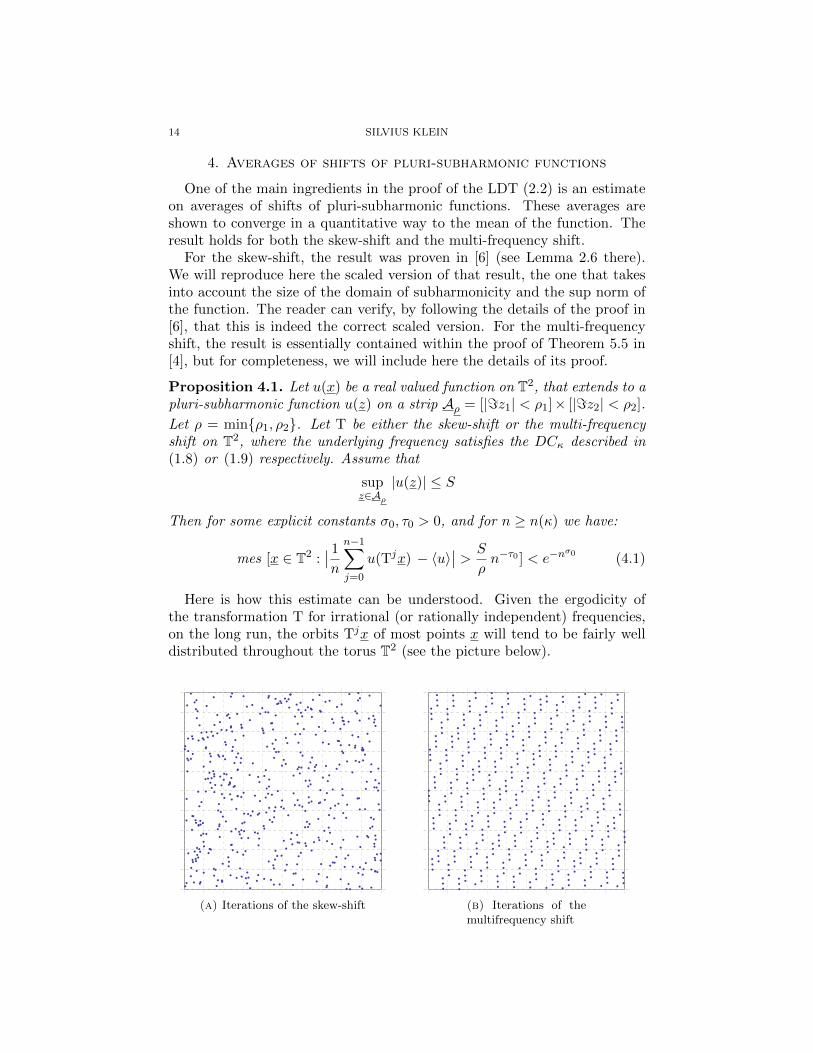
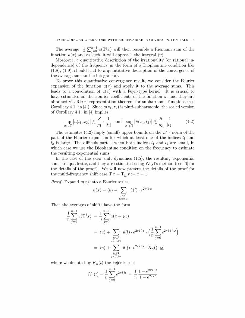
Here is how this estimate can be understood. Given the ergodicity ofthe transformation T for irrational (or rationally independent) frequencies,on the long run, the orbits Tjx of most points x will tend to be fairly welldistributed throughout the torus T2 (see the picture below).

(a) Iterations of the skew-shift (b) Iterations of themultifrequency shift


The average 1n

∑n−1j=0 u(Tjx) will then resemble a Riemann sum of the

function u(x) and as such, it will approach the integral 〈u〉.Moreover, a quantitative description of the irrationality (or rational in-

dependence) of the frequency in the form of a Diophantine condition like(1.8), (1.9), should lead to a quantitative description of the convergence ofthe average sum to the integral 〈u〉.

To prove this quantitative convergence result, we consider the Fourierexpansion of the function u(x) and apply it to the average sums. Thisleads to a convolution of u(x) with a Fejer-type kernel. It is crucial tohave estimates on the Fourier coefficients of the function u, and they areobtained via Riesz’ representation theorem for subharmonic functions (seeCorollary 4.1. in [4]). Since u(z1, z2) is pluri-subharmonic, the scaled versionof Corollary 4.1. in [4] implies:

supx2∈T

∣∣u(l1, x2)∣∣ . S

ρ1· 1

|l1|and sup

x1∈T

∣∣u(x1, l2)∣∣ . S

ρ2· 1

|l2|(4.2)

The estimates (4.2) imply (small) upper bounds on the L2 - norm of thepart of the Fourier expansion for which at least one of the indices l1 andl2 is large. The difficult part is when both indices l1 and l2 are small, inwhich case we use the Diophantine condition on the frequency to estimatethe resulting exponential sums.

In the case of the skew shift dynamics (1.5), the resulting exponentialsums are quadratic, and they are estimated using Weyl’s method (see [6] forthe details of the proof). We will now present the details of the proof forthe multi-frequency shift case Tx = Tω x := x+ ω.

Proof. Expand u(x) into a Fourier series

u(x) = 〈u〉+∑l∈Z2l 6=(0,0)

u(l) · e2πi l·x

Then the averages of shifts have the form

1

n

n−1∑j=0

u(Tjx) =1

n

n−1∑j=0

u(x+ jω)

= 〈u〉+∑l∈Z2l 6=(0,0)

u(l) · e2πi l·x ·( 1

n

n−1∑j=0

e2πi j l·ω)

= 〈u〉+∑l∈Z2l 6=(0,0)

u(l) · e2πi l·x ·Kn(l · ω)

where we denoted by Kn(t) the Fejer kernel

Kn(t) =1

n

n−1∑j=0

e2πi jt =1

n

1− e2πi nt

1− e2πi t

16 SILVIUS KLEIN

which clearly has the bound∣∣Kn(t)∣∣ ≤ min

1,

1

n‖t‖

(4.3)

We then have:∥∥∥ 1

n

n−1∑j=0

u(x+ jω)− 〈u〉∥∥∥2

L2(T2)=

∑l∈Z2l6=(0,0)

∣∣u(l)∣∣2 · ∣∣Kn(l · ω)

∣∣2=

∑1≤|l|<K

∣∣u(l)∣∣2 · ∣∣Kn(l · ω)

∣∣2 +∑|l|≥K

∣∣u(l)∣∣2 · ∣∣Kn(l · ω)

∣∣2We will estimate the second sum above using the bounds (4.2) on the Fouriercoefficients of u(x) and the first sum using the DC (1.9) on the frequency ω.The splitting point K will be chosen to optimize the sum of these estimates.

Clearly (4.2) implies:∑l2∈Z

∣∣u(l1, l2)∣∣2 =

∥∥∥u(l1, x2)∥∥∥2

L2x2

(T).( Sρ1

1

|l1|

)2≤(Sρ

)2 1

|l1|2

and ∑l1∈Z

∣∣u(l1, l2)∣∣2 =

∥∥∥u(x1, l2)∥∥∥2

L2x1

(T).( Sρ2

1

|l2|

)2≤(Sρ

)2 1

|l2|2

Then we have: ∑|l|≥K

∣∣u(l)∣∣2 · ∣∣Kn(l · ω)

∣∣2 ≤ ∑|l|≥K

∣∣u(l)∣∣2

≤∑

l : |l1|≥K/2

∣∣u(l)∣∣2 +

∑l : |l2|≥K/2

∣∣u(l)∣∣2 .(S

ρ

)2 1

K

Estimate (4.2) clearly impies:∣∣u(l)∣∣ . S

ρ

1

|l|Then using the DC (1.9) on ω and (4.3), we obtain:∑

1≤|l|<K

∣∣u(l)∣∣2 · ∣∣Kn(l · ω)

∣∣2 ≤(Sρ

)2 ∑1≤|l|<K

1

|l|2· 1

n2 ‖l · ω‖2

≤(Sρ

)2 ∑1≤|l|<K

1

|l|2· |l|

2A

n2 κ2.(Sρ

)2 K2A

n2κ2

We conclude:∥∥∥ 1

n

n−1∑j=0

u(x+ jω)− 〈u〉∥∥∥L2(T2)

≤ S

ρ

( 1

K1/2+KA

nκ

)≤ S

ρn−a

for some positive constant a that depends on A and for n large enoughdepending on A and κ.


Using Chebyshev’s inequality, the above estimate implies:

mes [x ∈ T2 :∣∣ 1n

n−1∑j=0

u(x+ jω) − 〈u〉∣∣ > S

ρn−a/3] < n−4a/3 (4.4)

This is not exactly what we wanted, since the size of the “bad” set abovedecays only polynomially fast in n, instead of exponentially fast.

To boost this estimate, we will use Lemma 4.12 in J. Bourgain’s mono-graph [4]. This result shows that a weaker a-priori estimate on a subhar-monic function implies an upper bound on its BMO norm, which in turnleads, via John-Nirenberg inequality, to a stronger estimate on the function.We reproduce here a “rescaled” version of the estimate in [4], one that takesinto account the width ρ of subharmonicity. The reader may verify that thisis indeed the correct rescaled version of the statement.

Lemma 4.1. Assume that u = u(x) : T2 → R has a pluri-subharmonicextension u(z) on Aρ = [|=z1| < ρ1]×[|=z2| < ρ2] such that sup

z∈Aρ

∣∣u(z)∣∣ ≤ B.

Let ρ = minρ1, ρ2. If

mes [x ∈ T2 :∣∣u(x)− 〈u〉

∣∣ > ε0] < ε1 (4.5)

then for an absolute constant c > 0,

mes [x ∈ T2 :∣∣u(x)− 〈u〉

∣∣ > ε01/4] < e

−c(ε01/4+

√Bρε1

1/4

ε01/2

)−1

(4.6)

We will apply this result to the average

u](x) :=ρ

S

1

n

n−1∑j=0

u(x+ jω)

Clearly u](x) is pluri-subharmonic on the same strip Aρ as u(x), its upper

bound on this strip is B = ρ and its mean is⟨u]⟩=ρ

S〈u〉

Then (4.4) implies

mes [x ∈ T2 :∣∣u](x)−

⟨u]⟩∣∣ > ε0] < ε1 (4.7)

where ε0 := n−a/3 and ε1 := n−4a/3 so ε1 ε0.Applying Lemma 4.1 and performing the obvious calculations, from in-

equality (4.6) we get

mes [x ∈ T2 :∣∣u](x)−

⟨u]⟩∣∣ > n−a/12] < e−c n

a/12

which then implies (4.1) for the multi-frequency shift Tω.

18 SILVIUS KLEIN

5. Lojasiewicz inequality for multivariable smooth functions

To prove the large deviation estimate (2.2) for a large enough initialscale N0, we will need a quantitative description of the transversality con-dition (1.12). More precisely, we will show that if a smooth function v(x) isnot flat at any point as defined in (1.12), then the set [x : v(x) ≈ E] of pointswhere v(x) is almost constant has small measure (and bounded complexity).

Such an estimate is called a Lojasiewicz type inequality and it is alreadyavailable for non-constant analytic functions. For such functions it can bederived using complex analysis methods from [20], namely lower bounds forthe modulus of a holomorphic function on a disk (see Lemma 11.4 in [12]).

For non-analytic functions, the proof is more difficult. Using Sard-typearguments, we have obtained a similar result for one-variable functions (seeLemma 5.3 in [16]). For multivariable smooth functions, the argument ismore technical and it involves a quantitative form of the implicit functiontheorem, also used in [7] and [14].

We begin with a simple compactness argument that shows that in theTC (1.12) we can work with finitely many partial derivatives.

Lemma 5.1. Assume v(x) is a smooth, 1-periodic function on R2. Thenv(x) satisfies the transversality condition (1.12) if and only if

∃m ∈ N2 |m| 6= 0 ∃c > 0 : ∀x ∈ T2 maxα≤m|α|6=0

∣∣∂α v(x)∣∣ ≥ c (5.1)

The constants m, c in (5.1) depend only on v.

Proof. Clearly (5.1)⇒ (1.12). We prove the converse. The TC (1.12) implies

∀x ∈ T2 ∃mx ∈ N2∣∣mx

∣∣ 6= 0 such that∣∣∂mx v (x)

∣∣ > cx > 0

Then there are radii rx > 0 so that if y is in the disk D(x, rx) we have∣∣∂mx v (y)∣∣ ≥ cx > 0. The family D(x, rx) : x ∈ T2 covers T2. Consider a

finite subcover D(x1, rx1), . . . , D(xk, rxk). Let m ∈ N2 such that m ≥ mxj

for all 1 ≤ j ≤ k and c := min1≤j≤k

cxj . Then (5.1) follows.

The following is a more precise form of the implicit function theorem(which was also used in [14]).

Lemma 5.2. Let f(x) be a C1 function on a rectangle R = I × J ⊂ [0, 1]2,let J = [c, d] and A := max

x∈R|∂x1f(x)|. Assume that

minx∈R|∂x2f(x)| =: ε0 > 0 (5.2)

If f(a1, a2) = 0 for some point (a1, a2) ∈ R, then there is an interval I0 =(a1 − κ, a2 + κ) ⊂ I and a C1 function φ0(x1) on I0 such that:

(i) f(x1, φ0(x1)) = 0 for all x1 ∈ I0

(ii) |∂x1φ0(x1)| ≤ Aε−10

(iii) x1 ∈ I0 and f(x1, x2) = 0 =⇒ x2 = φ0(x1)


Moreover, the size κ of the domain of φ0 can be taken as large as κ ∼ε0A

−1 ·mina2 − c, d− a2.

Proof. From (5.2), since ∂x2f(x) is either positive on R or negative on R(in which case replace f by −f), we may clearly assume that in fact:

minx∈R

∂x2f(x) =: ε0 > 0 (5.3)

Moreover, note that for any fixed x1 ∈ I, since ∂x2f(x1, x2) 6= 0, theequation f(x1, x2) = 0 has a unique solution x2.

Let x1 ∈ I0. Then∣∣f(x1, a2)∣∣ =

∣∣f(x1, a2)− f(a1, a2)∣∣ =

∣∣∂x1f(ξ, a2)∣∣ · |x1 − a1| ≤ Aκ

We have two possibilities.

0 ≤ f(x1, a2) ≤ Aκ. Then, if a2 − t ∈ J we have:

f(x1, a2 − t)− f(x1, a2) = ∂x2f(x1, ξ) · (−t)f(x1, a2 − t) = f(x1, a2)− t · ∂x2f(x1, ξ) ≤ Aκ− tε0 = 0

provided t = Aε−10 κ

For this choice of t, a2 − t is indeed in J , because of the size κ0 of theinterval I0: t = Aε−1

0 κ ≤ Aε−10 ε0A

−1(a2 − c) = a2 − c, so a2 − t ≥ c.Therefore,

f(x1, a2 − t) ≤ 0 ≤ f(x1, a2)

so there is a unique x2 =: φ0(x1) ∈ [a2 − t, a2] such that f(x1, φ0(x1)) = 0.

−Aκ ≤ f(x1, a2) ≤ 0. Then, if a2 + t ∈ J we have:

f(x1, a2 + t)− f(x1, a2) = ∂x2f(x1, ξ) · tf(x1, a2 + t) = f(x1, a2) + t · ∂x2f(x1, ξ) ≥ −Aκ+ tε0 = 0

provided t = Aε−10 κ

As before, for this choice of t, a2 + t is in J , because of the size κ of theinterval I0: t = Aε−1

0 κ ≤ Aε−10 ε0A

−1(d− a2) = d− a2, so a2 + t ≤ d.

Therefore,f(x1, a2) ≤ 0 ≤ f(x1, a2 + t)

so there is a unique x2 =: φ0(x1) ∈ [a2, a2 + t] such that f(x1, φ0(x1)) = 0.

We proved (i) and (iii). The fact that φ0(x1) is C1 follows from the stan-dard implicit function theorem, while the estimate (ii) follows immediatelyfrom (i) using the chain’s rule.

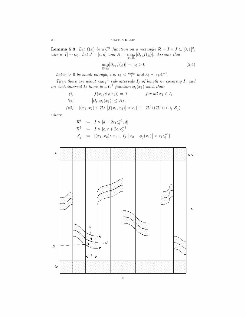
The following is a quantitative and global version of the previous lemma(see also Lemma 8.3 in [14]). It says that under the same conditions asabove, the points (x1, x2) ∈ R for which

∣∣f(x1, x2)∣∣ ≤ ε are either in a

narrow strip at the top or at the bottom of the rectangle R, or near thegraphs of some functions φj(x1), in other words x2 ≈ φj(x1).

20 SILVIUS KLEIN

Lemma 5.3. Let f(x) be a C1 function on a rectangle R = I × J ⊂ [0, 1]2,where |I| ∼ κ0. Let J = [c, d] and A := max

x∈R|∂x1f(x)|. Assume that:

minx∈R

∣∣∂x2f(x)∣∣ =: ε0 > 0 (5.4)

Let ε1 > 0 be small enough, i.e. ε1 <ε0κ0

4 and κ1 ∼ ε1A−1.

Then there are about κ0κ−11 sub-intervals Ij of length κ1 covering I, and

on each interval Ij there is a C1 function φj(x1) such that:

(i) f(x1, φj(x1)) = 0 for all x1 ∈ Ij(ii)

∣∣∂x1φj(x1)∣∣ ≤ Aε−1

0

(iii) [(x1, x2) ∈ R :∣∣f(x1, x2)

∣∣ < ε1] ⊂ Rt ∪Rb ∪ (∪j Sj)where

Rt := I × [d− 2ε1ε−10 , d]

Rb := I × [c, c+ 2ε1ε−10 ]

Sj := [(x1, x2) : x1 ∈ Ij ,∣∣x2 − φj(x1)

∣∣ < ε1ε−10 ]


Proof. Divide the interval I, whose length is ∼ κ0 into ∼ κ0κ−11 sub-intervals

Ij of length κ1 each.

If∣∣f(x1, x2)

∣∣ ≥ ε1 for all (x1, x2) ∈ Ij × [c + 2ε1ε−10 , d − 2ε1ε

−10 ], then we

are done with the interval Ij .Otherwise, assume

∣∣f(a1, a2)∣∣ < ε1 for some a1 ∈ Ij and a2 ∈ [c +

2ε1ε−10 , d− 2ε1ε

−10 ].

We may assume 0 ≤ f(a1, a2) ≤ ε1, the other case being treated similarly.Then if a2 − t ∈ J we have:

f(a1, a2 − t)− f(a1, a2) = ∂x2f(a1, ξ) · (−t) for some ξ ∈ (a2 − t, a2)

f(a1, a2 − t) = f(a1, a2)− t · ∂x2f(a1, ξ) ≤ ε1 − ε0t = 0

provided t = ε1ε−10 . Since a2 ≥ c+ 2ε1ε

−10 , for this t we have a2 − t ∈ J .

We then have f(a1, a2 − t) ≤ 0 ≤ f(a1, a2), so f(a1, a∗2) = 0 for some

a∗2 ∈ [a2 − t, a2].We can use Lemma 5.2 around the point (a1, a

∗2). The interval we get has

length at least ε0A−1 ·mina2− c, d− a2 > ε0A

−1 · 2ε1ε−10 = 2ε1A

−1 > 2κ1,so it contains Ij , whose length is ∼ κ1. We have a C1 function φj on Ij such

that |∂x1φj | ≤ Aε−10 and

x1 ∈ Ij and f(x1, x2) = 0 ⇐⇒ x2 = φj(x1)

Now let (x1, x2) ∈ R such that∣∣f(x1, x2)

∣∣ < ε1. Then either (x1, x2) ∈Rt ∪Rb or (x1, x2) ∈ Ij × [c+ 2ε1ε

−10 , d− 2ε1ε

−10 ] for some j, in which case:

ε1 >∣∣f(x1, x2)

∣∣ = |f(x1, x2)− f(x1, φj(x1))| =

= |∂x2f(x1, ξ)| · |x2 − φj(x1)| ≥ ε0 · |x2 − φj(x1)|from which we conclude that |x2 − φj(x1)| < ε1ε

−10 .

We have shown that the points x = (x1, x2) ∈ R for which |f(x)| < ε1 arewithin ∼ ε1 from the graphs of some functions φj(x1) that have boundedslopes and are defined on small intervals Ij . This shows that the ’bad’set [x ∈ R : |f(x)| < ε1] can be covered by small rectangles instead of ε1-neighborhoods of curves, and we have control on the size of these rectanglesand on their number. In turn, the ’good’ set [x ∈ R : |f(x)| ≥ ε1] can becovered by a comparable number of rectangles, which can be further choppeddown into squares, to preserve the symmetry between the two variables. Thisis the content of the following lemma.

Lemma 5.4. Given a C2 function f(x) on a square R0 = I0× J0 ⊂ [0, 1]2,where |I0|, |J0| ∼ κ0. Denote A := max

|α|≤2maxx∈R|∂αf(x)|. Assume that:

minx∈R0

|∂x2f(x)| =: ε0 > 0 or minx∈R0

|∂x1f(x)| =: ε0 > 0 (5.5)

Let ε1 > 0 be small enough, i.e. ε1 <ε0κ0

4 and κ1 ∼ ε1A−1.

22 SILVIUS KLEIN

Then there is a set B1 ⊂ R0, with

mes [B1] . κ0 ε1 ε−10 (5.6)

such that R0 \ B1 is a union of about (κ0 κ−11 )2 squares, where each such

square has the form R1 = I1 × J1, with∣∣I1

∣∣, ∣∣J1

∣∣ ∼ κ1.For each of these squares we have:

minx∈R1

∣∣f(x)∣∣ ≥ ε1 (5.7)

Proof. We will use Lemma 5.3. I0 is covered by about κ0κ−11 subintervals Ij

of length κ1. Consider one such subinterval. There is a C1 function φj(x1)

on Ij such that |∂x1φj(x1)| ≤ Aε−10 and

[(x1, x2) ∈ Ij × J0 :∣∣f(x1, x2)

∣∣ < ε1] ⊂ Rtj ∪Rbj ∪ Sjwhere if J0 = [c0, d0] then

Rtj := Ij × [d0 − 2ε1ε−10 , d0]

Rbj := Ij × [c0, c0 + 2ε1ε−10 ]

Sj := [(x1, x2) : x1 ∈ Ij , |x2 − φj(x1)| < ε1ε−10 ]

Then

Sj ⊂ Ij × [ minx1∈Ij

φj(x1)− ε1ε−10 , max

x1∈Ijφj(x1) + ε1ε

−10 ] =: Ij ×Km

j =: Rmj

For any x1, x′1 ∈ Ij we have∣∣φj(x1)− φj(x′1)

∣∣ . Aε−10 ·

∣∣x1 − x′1∣∣ ≤ Aε−1

0 κ1 ∼ ε1ε−10

which shows that ∣∣Kmj

∣∣ . ε1ε−10

We have shown that [(x1, x2) ∈ Ij × J0 :∣∣f(x1, x2)

∣∣ < ε1] is covered by

three rectangles: Rtj , Rbj , Rmj , each of the form Ij × Kj where∣∣Ij∣∣ ∼ κ1,∣∣Kj

∣∣ ∼ ε1ε−10 .

Summing over j . κ0κ−11 , we get that the set [x ∈ R0 :

∣∣f(x)∣∣ < ε1] is

contained in the union B1 of about κ0κ−11 rectangles of size κ1×ε1ε−1

0 . Then

mes [B1] . κ0κ−11 · κ1 · ε1ε−1

0 = κ0ε1ε−10

which proves (5.6).

The complement of this set, R0 \ B1, consists of about the same numberκ0κ

−11 of rectangles - this was the reason for switching from ε1-neighborhoods

of curves to rectangles. Each of these rectangles has the form Ij×Lj , where∣∣Ij∣∣ ∼ κ1 and∣∣Lj∣∣ ∼ κ0−O(ε1ε

−10 ) ∼ κ0 κ1. Divide each of these vertical

rectangles into about κ0κ−11 squares of size κ1 × κ1 each.

We conclude that R0 \ B1 is covered by about (κ0κ−11 )2 squares of the

form R1 = I1 × J1, where the size of each square is∣∣I1

∣∣, ∣∣J1

∣∣ ∼ κ1.


We now have all the ingredients for proving the following Lojasiewicz typeinequality.

Theorem 5.1. Assume that v(x) is a smooth function on [0, 1]2 satisfyingthe transversality condition (1.12). Then for every ε > 0

supE∈R

mes [x ∈ [0, 1]2 : |v(x)− E| < ε] < C · εb (5.8)

where C, b > 0 depend only on v.

Proof. Using Lemma 5.1,

∃m = (m1,m2) ∈ N2 |m| 6= 0 ∃c > 0 : ∀x ∈ T2 maxα≤m|α|6=0

∣∣∂α v(x)∣∣ ≥ c

Let

A := maxα≤(m1+1,m2+1)

maxx∈[0,1]2

∣∣∂α v(x)∣∣

We may of course assume that∣∣E∣∣ ≤ 2A, otherwise there is nothing to

prove.All the constants in the estimates that follow will depend only on |m| , c, A

(so in particular only on v).

Partition [0, 1]2 into about (2Ac )2 squares of the form R = I × J of size∣∣I∣∣, ∣∣J∣∣ ∼ c

2A .Let R be such a square. Then either |v(x)| ≥ ε for all x ∈ R, in which

case we are done with this square, or for some a = (a1, a2) ∈ R we have|v(a)| < ε. But then for one of the partial derivatives α ≤ m, |α| 6= 0, wehave

∣∣∂α v(a)∣∣ ≥ c.

Assume for simplicity that∣∣∂m v(a)

∣∣ ≥ c, which is the worst case scenario.If x ∈ R, then ‖x− a‖∞ := max|x1 − a1| , |x2 − a2| ≤ c

2A .Then∣∣∂m v(x)− ∂m v(a)

∣∣ . maxy∈R

∣∣∇∂m v(y)∣∣ · ‖x− a‖∞ ≤ A · c

2A=c

2

It follows that

minx∈R

∣∣∂m v(x)∣∣ & c

2

We will use Lemma 5.4 |m| =: m times.

Step 1. Let

f1(x) := ∂(m1,m2−1) v(x)

Then

minx∈R

∣∣∂x2f1(x)∣∣ = min

x∈R

∣∣∂m v(x)∣∣ & c

We apply Lemma 5.4 to the function f1 with the following data:

R0 = R, κ0 =c

2A, ε0 ∼ c, ε1 <

ε0κ0

4, κ1 ∼ ε1A−1

where ε1 will be chosen later.

24 SILVIUS KLEIN

We get a set B[1 := B1, mes [B[1] . κ0ε1ε−10 < κ2

0A · ε1ε−20 such that

R0 \ B[1 is a union of about (κ0κ−11 )2 squares of the form R1 = I1 × J1, of

size∣∣I1

∣∣, ∣∣J1

∣∣ ∼ κ1. For each of these squares we have:

minx∈R1

∣∣f1(x)∣∣ ≥ ε1

which means:

minx∈R1

∣∣ ∂(m1,m2−1) v(x)∣∣ ≥ ε1

Step 2. Pick any of the squares R1 = I1 × J1 from the previous stepand consider say

f2(x) := ∂(m1−1,m2−1) v(x)

Then

minx∈R1

∣∣∂x1f2(x)∣∣ = min

x∈R1

∣∣∂(m1,m2−1) v(x)∣∣ ≥ ε1

Apply Lemma 5.4 to the function f2 with the following data:

R1, κ1, ε1 from Step 1, ε2 <ε1κ1

4 , κ2 ∼ ε2A−1

where ε2 will be chosen later.We get a set B2, mes [B2] . κ1ε2ε

−11 such that R1\B2 is a union of about

(κ1κ−12 )2 squares of the form R2 = I2 × J2, of size

∣∣I2

∣∣, ∣∣J2

∣∣ ∼ κ2. For eachof these squares we have:

minx∈R2

∣∣f2(x)∣∣ ≥ ε2

which means:

minx∈R2

∣∣ ∂(m1−1,m2−1) v(x)∣∣ ≥ ε2

If we do this for each of the ∼ (κ0κ−11 )2 squares resulting from Step 1,

and if we put together all the ‘bad’ sets B2 corresponding to each of thesesquares, we conclude the following.

There is a set B[2 ⊂ R such that:

mes [B[2] . κ1ε2ε−11 · (κ0κ

−11 )2 = κ0ε2ε

−11 κ−1

1 ∼ κ20A · ε2ε−2

1

Hence the total measure of the ‘bad’ set in Step 2 is:

mes [B[2] . κ20A · ε2ε−2

1

Moreover, R \ (B[1 ∪ B[2) is covered by squares of the form R2 = I2 × J2,of size

∣∣I2

∣∣, ∣∣J2

∣∣ ∼ κ2.The total number of such squares is about

(κ1κ−12 )2 · (κ0κ

−11 )2 = (κ0κ

−12 )2

On each of these squares we have:

minx∈R2

∣∣ ∂(m1−1,m2−1) v(x)∣∣ ≥ ε2


It is clear how this procedure continues. Perform it for m− 1 steps. Wewill get sets B[1, . . . ,B[m−1 such that R\ (B[1 ∪ . . .∪B[m−1) consists of about

(κ0κ−1m−1)2 squares of the formRm−1 = Im−1×Jm−1, of size

∣∣Im−1

∣∣, ∣∣Jm−1

∣∣ ∼κm−1. On each of these squares we have

minx∈Rm−1

∣∣ ∂x2 v(x)∣∣ ≥ εm−1 or min

x∈Rm−1

∣∣ ∂x1 v(x)∣∣ ≥ εm−1

Step m. Assume the former inequality above and apply Lemma 5.4one more time. Let

fm(x) := v(x)− Efor some fixed energy E with

∣∣E∣∣ ≤ 2A (the estimates will not depend onE). Then for each of the squares Rm−1 from the previous step we have:

minx∈Rm−1

∣∣∂x2 fm(x)∣∣ = min

x∈Rm−1

∣∣∂x2 v(x)∣∣ ≥ εm−1

Apply Lemma 5.4 to the function fm with the following data:

Rm−1, κm−1, εm−1 from the previous step, εm < εm−1κm−1

4 , κm ∼ εmA−1

where εm will be chosen later.We get a set Bm, mes [Bm] . κm−1εmε

−1m−1 such that Rm−1 \ Bm is a

union of about (κm−1κ−1m )2 squares of the form Rm = Im × Jm, of size∣∣Im∣∣, ∣∣Jm∣∣ ∼ κm. For each of these squares we have:

minx∈Rm

∣∣fm(x)∣∣ ≥ εm

which means:

minx∈Rm

∣∣v(x)− E∣∣ ≥ εm

If we do this for each of the ∼ (κ0κ−1m−1)2 squares resulting from the

previous step, and if we put together all the corresponding ‘bad’ sets, weconclude.

There is a set B[m ⊂ R such that:

mes [B[m] . κm−1εmε−1m−1 · (κ0κ

−1m−1)2 = κ0εmε

−1m−1κ

−1m−1 ∼ κ

20A · εmε−2

m−1

Hence the total measure of the ‘bad’ set in Step m is:

mes [B[m] . κ20A · εmε−2

m−1

Moreover, R\ (B[1 ∪B[2 . . .∪B[m) is covered by squares of the form Rm =Im × Jm, of size

∣∣Im∣∣, ∣∣Jm∣∣ ∼ κm.The total number of such squares is about

(κm−1κ−1m )2 · (κ0κ

−1m−1)2 = (κ0κ

−1m )2

On each of these squares we have:

minx∈Rm

∣∣v(x)− E∣∣ ≥ εm

26 SILVIUS KLEIN

Therefore, the total measure of the bad set from all steps is:

mes [B[1 ∪ B[2 . . . ∪ B[m] . κ20A · [ε1ε−2

0 + ε2ε−21 + . . . εmε

−2m−1] (5.9)

We choose

εj := ε1/3m−j

for 1 ≤ j ≤ m

If ε < ε∗(c,m), then ε0 ∼ c > ε1/3m

, ε−20 ∼ c−2 < ε−2, so there is no harm

in also putting (for simplicity) ε0 = ε1/3m

.It is a simple calculation to see that for any ε < ε∗(m,A), we have εj+1 <

εjκj4 for all j = 0 . . .m− 1, which allows our inductive process to work.

Note that ε3j = εj+1 so εj+1ε−2j = εj . This implies:

ε1ε−20 + ε2ε

−21 + . . . εmε

−2m−1 = ε0 + ε1 + . . .+ εm−1 ≤ mε0 = m · ε1/3m

From (5.9) it follows that the total measure of the bad set inside thesquare R is:

mes [B[1 ∪ B[2 . . . ∪ B[m] . κ20Am · ε1/3

m

There are about (2Ac )2 = κ−2

0 such squares.

We conclude that outside a bad set B, mes [B] < Am · e1/3m , we have∣∣v(x)− E∣∣ ≥ ε, which proves (5.1) with C ∼ Am and b = 1

3m .

Remark 5.1. The exponent b in (5.8) is related to the Lojasiewicz exponentof the function v (see [17], [10]). Determining the optimal exponent insuch an inequality is an interesting problem in itself, and has been studiedextensively for polynomials and analytic functions. It is clear that for apolynomial, the Lojasiewicz exponent should be related to its degree d, andit is in fact shown to be O( 1

d2) with explicit underlying constants (see [10],

[17]). The proof of the Lojasiewicz inequality for analytic functions in [12](see Lemma 11.4 there) does not provide an explicit value for the exponent,but Theorem 4 in [21] provides a scheme for computing it via the Newtondistance of v.

In our proof for smooth, transversal functions, we obtain the exponent 13m ,

where m is the maximum number of partial derivatives needed for transver-sality. If v were a polynomial of degree d, then m would be d, which showsthat our estimate is very wasteful (we have obtained a better estimate,O( 1

m), for one-variable functions, see Lemma 5.3 in [16]). This, however,seems to be the only such estimate available now for non-analytic functionsof two variables.

A similar argument can be made for functions of more than two variables,so (5.8) will hold for such functions as well.


6. Large deviation theorem, the proof of main results

Using induction on the scale N , we will prove the large deviation esti-mate (2.2) for the logarithmic average of transfer matrices:

mes [x ∈ T2 :∣∣ 1

Nlog‖MN (x,E)‖ − LN (E)

∣∣ > N−τ ] < e−Nσ

as well as a lower bound on the mean of these quantities:

LN (E) ≥ γN log |λ|The base step of the induction uses the quantitative description (5.8) of

the transversality condition (1.12) on the potential function, and the largesize of the coupling constant. The inductive step uses only the regularity ofthe potential function via Lemma 3.1, which provides a good approximationof these logarithmic averages by pluri-subharmonic functions.

Lemma 6.1. (Base step of the induction) Assume that v(x) is smooth andsatisfies the transversality condition (1.12). Then given any constant C > 0,there are positive constants λ1 and B which depend on v and C, such thatfor any scale N0, for any λ subject to |λ| ≥ maxλ1, N

B0 and for any E ∈ R

we have:

mes [x ∈ T2 :∣∣ 1

N0log‖MN0(x, λ,E)‖ − LN0(λ,E)

∣∣ > 1

20S(λ) ] < N−C0

(6.1)Furthermore, for these λ, N0 and for all E we have:

LN0(λ,E) ≥ 1

2S(λ) (6.2)

LN0(λ,E)− L2N0(λ,E) ≤ 1

80S(λ) (6.3)

Proof. The proof of this result is similar to the analytic potential func-tion case. That is because the only fact about analyticity needed here isthe Lojasiewicz inequality (5.8), which holds for any non-constant analyticfunctions, and which we have established in section 5 for smooth functionssatisfying the transversality condition (1.12). We will then omit the proof,but the reader is referred to the proof of Lemma 2.10 in [6] for details.

We will now explain the idea of the proof of the inductive step.If at scale N0 we apply the almost invariance property (3.18) n times and

then average, we get:∣∣LN0(x)− 1

n

n−1∑j=0

LN0(Tjx)∣∣ . nS(λ)

N0(6.4)

so using the approximation (3.16), we also get:∣∣uN0(x)− 1

n

n−1∑j=0

uN0(Tjx)∣∣ . nS(λ)

N0(6.5)

28 SILVIUS KLEIN

To have a decay above, we need to take a smaller number of shifts n N0.Apply the estimate (4.1) on averages of shifts of pluri-subharmonic func-

tions to uN0(x) and get:

mes [x ∈ T2 : | 1

n

n−1∑j=0

uN0(Tjx) − 〈uN0〉 | >S

ρN0

n−τ0 ] < e−nσ0

(6.6)

We may combine (6.5), (6.6) to directly obtain a large deviation estimatefor uN0(x) and then, via the approximations (3.16), (3.17) to obtain theLDT for LN0(x), only when the deviation S

ρN0n−τ0 1. In other words, this

approach works only when the scaling factor SρN0

is not too large to cancel the

decay n−τ0 . This is the case of the single or multi-frequency shift model withanalytic potential (see [4], [5]) where S

ρN0= S

ρ is just a constant depending on

the potential function v. This approach also works for the single-frequencymodel with potential function in a Gevrey class of order s < 2, since inthis case sharper estimates than (6.6) are available for averages of shifts ofsingle-variable subharmonic functions (see [16]). This approach fails for theskew-shift model (whether the potential function is analytic or Gevrey) andalso for the multi-frequency model with Gevrey potential function, becausethe size ρN0 of the subharmonic extension depends on the scale N0.

Therefore, in order to beat the scaling factor SρN0

when applying the

estimate (6.6) to a transfer matrix substitute uN0(x) at scale N0, we needto consider a large number of shifts n N0. The averages of shifts thusobtained will be close to the mean 〈uN0〉. Moreover, we will get:

LN0

(1)≈ 〈uN0〉

(2)≈ 1

n

n−1∑j=0

uN0(Tjx)

(3)≈ 1

n

n−1∑j=0

1

N0log‖MN0(Tjx)‖

(4)≈ 1

nN0log‖MnN0(x)‖

The first approximation above is just (3.17). The second is exactly (6.6).The third is due to (3.16). The last approximation above essentially saysthat:

n−1∏j=0

‖MN0(Tjx)‖ ≈ ‖n−1∏j=0

MN0(Tjx)‖ ≈ ‖MnN0(x)‖

or in other words, that the product of the norms of certain transfer matricesis approximately equal to the norm of the product of these matrices, thelatter giving us the transfer matrix at the larger scale nN0.

If these heuristics were true, then for n N0 we would get

LN0 ≈1

nN0log‖MnN0(x)‖


which would establish the large deviation estimate for transfer matrices ata larger scale nN0.

The avalanche principle, which is a deterministic result, describes howestimates on the norms of individual (and of products of two consecutive)SL2(R) matrices can lead to estimates on the norm of the product of allmatrices (see [12], [4]), thus providing the basis for establishing the aboveheuristics. It requires a uniform lower bound on the norms of individualmatrices in the product, as well as knowing that the norm of the product ofany two consecutive matrices is comparable to the product of their norms.

The following lemma provides the inductive step in proving the LDT foran increasing sequence of scales N . It also provides the inductive step inproving the positivity and continuity of the Lyapunov exponent. The proofof this lemma is based on the heuristics described above, and combines theaverages of shifts estimate (4.1), the almost invariance property (3.18) andthe avalanche principle (see Proposition 2.2 in [12]).

Before stating the lemma let us describe the various parameters and con-stants that will appear.

List of constants and parameters:

s > 1 is the order of the Gevrey class.δ = 2(s− 1) refers to the size (≈ N−δ) of the holomorphic extensions of

the transfer matrix substitutes.D := 2δ + 8, A := max2 (δ+1)

τ0, 2 are some well chosen powers of the

scale N , τ0 is the exponent from (4.1).γ > 1

4 is a fixed number.

Note that all these constants are either universal or depend on the orders of the Gevrey class.

λ, E are fixed parameters such that∣∣E∣∣ ≤ ∣∣λ∣∣B+2, and B := sup

x∈T

∣∣v(x)∣∣.

The transformation T = Sω where ω ∈ DCκ or T = Tω where ω ∈ DCκfor some κ > 0.

N00 = N00(s, κ,B) is a sufficiently large integer, such that the asymptoticbehavior of various powers and exponentials applies to N00 and such that(4.1) holds for N00 shifts.

Lemma 6.2. (The inductive step) Consider two scales N0 and N such thatN0 ≥ N00, (3.16) holds at scale N0, that is:

N0 ≥ S(λ) ⇔ |λ| ≤ eN0 (6.7)

and

NA0 ≤ N ≤ eN0 (6.8)

Assume that a weak LDT holds at scales N0 and 2N0:

mes [x ∈ T2 :∣∣ 1

N0log‖MN0(x, λ,E)‖−LN0(λ,E)

∣∣ > γ

10S(λ)] < N−D (6.9)

30 SILVIUS KLEIN

mes [x ∈ T2 :∣∣ 1

2N0log‖M2N0(x, λ,E)‖ − L2N0(λ,E)

∣∣ > γ

10S(λ)] < N−D

(6.10)and that the means LN0, L2N0 have a lower bound and are close to eachother:

LN0(λ,E), L2N0(λ,E) ≥ γS(λ) (6.11)

LN0(λ,E)− L2N0(λ,E) ≤ γ40S(λ) (6.12)

Then similar (but stronger) estimates hold at the larger scale N :

mes [x ∈ T2 :∣∣ 1

Nlog‖MN (x, λ,E)‖ − LN (λ,E)

∣∣ > S(λ)N−τ ] < e−Nσ

(6.13)

LN (λ,E) ≥ γS(λ) (6.14)

−2[LN0(λ,E)− L2N0(λ,E)]− C0S(λ)N0N−1

LN (λ,E)− L2N (λ,E) ≤ C0S(λ)N0N−1 (6.15)

for some positive absolute constants C0, τ, σ.

Proof. The parameters λ, E and the transformation T = Sω or T = Tω

are fixed, so they can be suppressed from notations. For instance MN (x) =MN (x, λ,E), S(λ) = S etc.

We can assume without loss of generality that N is a multiple of N0,that is, that N = n ·N0. Indeed, if N = n ·N0 + r, 0 ≤ r < N0, then∣∣ 1


n ·N0log‖Mn·N0(x)‖

∣∣ ≤ 2SN0N−1 (6.16)

Therefore, if we prove (6.14), (6.15), (6.13) at scale n ·N0, then they holdat scale N too.

To prove (6.16), first note that MN (x) = B(x) ·Mn·N0(x), where

B(x) :=

n·N0+1∏j=N

A(Tjx) =

n·N0+1∏j=n·N0+r

A(Tjx)

so

‖B(x)‖ ≤ er·S ≤ eN0·S and ‖B(x)−1‖ ≤ er·S ≤ eN0·S

Since ‖Mn·N0(x)‖ ≥ 1 and ‖MN (x)‖ ≥ 1, it follows that:

1


n ·N0log‖Mn·N0(x)‖ =

1

n ·N0log‖MN (x)‖

n·N0N

‖Mn·N0(x)‖

≤ 1

n ·N0log‖B(x)‖

n·N0N · ‖Mn·N0(x)‖

n·N0N

‖Mn·N0(x)‖

≤ 1

n ·N0log (eN0S)

n·N0N = SN0N

−1


Similarly

1

n ·N0log‖Mn·N0(x)‖ − 1

Nlog‖MN (x)‖ =

1

n ·N0log||Mn·N0(x)||

‖MN (x)‖n·N0N

=1

n ·N0log [

(‖Mn·N0(x)‖||MN (x)||

)n·N0N · ‖Mn·N0(x)‖

rN ]

≤ 1

n ·N0log [ ‖(B(x))−1‖

n·N0N · ‖Mn·N0(x)‖

rN ]

≤ 1

n ·N0log [ (eN0S)

n·N0N · (enN0S)

N0N ] = 2SN0N

−1

and inequality (6.16) now follows.

We are going to show that (6.8) - (6.12) allow us to apply the avalanche

principle to the “blocks” MN0(T(j−1)N0 x), for j = 1, n. Each of these blocksis a product of N0 matrices, and they multiply up to MN (x).

Denote the set in (6.9) by BN0 and similarly the set in (6.10) by B2N0 .If x /∈ BN0 then using (6.9), (6.11) and (6.8) we get

‖MN0(x)‖ > e−γ10SN0+LN0

·N0 ≥ e9γ10SN0 =: µ > eN0 ≥ N > n

so

‖MN0(x)‖ ≥ µ ≥ n if x /∈ BN0 (6.17)

For 1 ≤ j ≤ n = NN0

consider Aj = Aj(x) := MN0(T(j−1)N0x). Then

(6.17) implies

min1≤j≤n

‖Aj(x)‖ ≥ µ for all x /∈n⋃j=0

T−jN0BN0 (6.18)

Since Aj+1(x) · Aj(x) = M2N0(T(j−1)N0x), using (6.9), (6.10), (6.12), forx /∈

⋃nj=0(T−jN0BN0) ∪

⋃nj=0(T−jN0B2N0) (which is a set of measure

< 2N−D ·N = 2N−D+1), we have :

log‖Aj+1(x)‖+ log‖Aj(x)‖ − log‖Aj+1(x) ·Aj(x)‖= log‖MN0(TjN0x)‖+ log‖MN0(T(j−1)N0x)‖ − log‖M2N0(T(j−1)N0x)‖

≤ N0(LN0 +Sγ

10) +N0(LN0 +

Sγ

10) + 2N0(

Sγ

10− L2N0)

= 2N0(LN0 − L2N0) +4Sγ

10N0 ≤

9Sγ

20N0 =

1

2logµ

Therefore,

log‖Aj+1(x)‖+ log‖Aj(x)‖ − log‖Aj+1(x) ·Aj(x)‖ ≤ 1

2logµ (6.19)

for x outside a set of measure < 2N−D+1.

32 SILVIUS KLEIN

Estimates (6.18), (6.19) are exactly the assumptions in the avalancheprinciple (Proposition 2.2 in [12]). We then conclude:∣∣log‖An(x) · . . . ·A1(x)‖+

n−1∑j=2

log‖Aj(x)‖ −n−1∑j=1

log‖Aj+1(x) ·Aj(x)‖∣∣ . n

µ

(6.20)for x outside a set of measure < 2N−D+1.

Hence, since N = n ·N0 and An(x) · . . . ·A1(x) = MN (x), we have:∣∣log‖MN (x)‖+

n−1∑j=2

log‖MN0(T(j−1)N0x)‖

−n−1∑j=1

log‖M2N0(T(j−1)N0x)‖∣∣ . n

µ

Therefore∣∣ 1

Nlog‖MN (x)‖+

1

n

n−1∑j=2

1

N0log‖MN0(T(j−1)N0x)‖

− 2

n

n−1∑j=1

1

2N0log‖M2N0(T(j−1)N0x)‖

∣∣ . 1

µ(6.21)

We will go from averages of n blocks in (6.21), to averages of N shifts.In (6.21) replace x by x,Tx, . . .TN0−1x and then average (i.e. add up allthese N0 inequalities and divide by N0) to get:∣∣ 1

N0

N0−1∑j=0

1

Nlog‖MN (Tjx)‖+

1

N

N−1∑j=0

1

N0log‖MN0(Tjx)‖

− 2

N

N−1∑j=0

1

2N0log‖M2N0(Tjx)‖

∣∣ . 1

µ(6.22)

The almost invariance property - Lemma (3.18) implies:∣∣ 1


N0

N0−1∑j=0

1

Nlog‖MN (Tjx)‖

∣∣ . SN0

N(6.23)

From (6.22) and (6.23) we get:∣∣ 1

Nlog‖MN (x)‖+

1

N

N−1∑j=0

1

N0log‖MN0(Tjx)‖

− 2

N

N−1∑j=0

1

2N0log‖M2N0(Tjx)‖

∣∣ . SN0

N+

1

µ. SN0N

−1 (6.24)

for x /∈ B1 :=⋃Nj=0(T−jBN0)∪

⋃nj=0(T−jB2N0) where mes [B1] < 2N−D+1.


Integrating the left hand side of (6.24) in x, we get:∣∣LN + LN0 − 2L2N0

∣∣ < CSN0N−1 + 4S · 2N−D+1 < C0SN0N

−1 (6.25)

LN + LN0 − 2L2N0 > −C0SN0N−1

LN > LN0 − 2(LN0 − L2N0)− C0SN0N−1

> γS − 2(LN0 − L2N0)− C0SN0N−1

which proves (6.14).Clearly all the arguments above work for N replaced by 2N , so we get

the analogue of (6.25) :∣∣L2N + LN0 − 2L2N0

∣∣ < C0SN0N−1 (6.26)

From (6.25) and (6.26) we obtain

LN − L2N ≤ C0SN0N−1

which is exactly (6.15).

To prove the LDT (6.13) at scale N , we are going to apply the estimate(4.1) on averages of shifts of pluri-subharmonic functions to the transfermatrix substitutes uN0 and u2N0 . Their widths of subharmonicity in each

variable are ρN0 , ρ2N0 ≈ N−δ−10 and they are uniformly bounded by S.

Using (3.16) which holds at scales N0 and 2N0 due to (6.7), we can ‘sub-stitute’ in (6.24) 1

N0log‖MN0(Tj(x)‖ by uN0(Tjx) and 1

2N0log‖M2N0(Tj(x)‖

by u2N0(Tjx) and get, for x /∈ B1:

∣∣ 1

Nlog‖MN (x)‖+

1

N

N−1∑j=0

uN0(Tjx)− 2

N

N−1∑j=0

u2N0(Tjx)∣∣ . SN0N

−1 (6.27)

Applying (4.1) to uN0 and u2N0 we get :

mes [x ∈ T2 :∣∣ 1

N

N−1∑j=0

uN0(Tjx)−〈uN0〉∣∣ > S ·N δ+1

0 ·N−τ0 ] < e−Nσ0

(6.28)

mes [x ∈ T2 :∣∣ 1

N

N−1∑j=0

u2N0(Tjx)− 〈u2N0〉∣∣ > S ·N δ+1

0 ·N−τ0 ] < e−Nσ0

(6.29)Denote the union of the two sets in (6.28), (6.29) by B2.Since N satisfies (6.8),

S ·N δ+10 ·N−τ0 < S · (N1/A)δ+1 ·N−τ0 < S ·N−τ1 where τ1 <

τ0

2

so from (6.27), (6.28), (6.29) we get:∣∣ 1

Nlog‖MN (x)‖ + 〈uN0〉 − 2 〈u2N0〉

∣∣. SN0N

−1 + S ·N−τ1 . S ·N−τ1 (6.30)

34 SILVIUS KLEIN

for x /∈ B := B1 ∪B2, where

mes [B] < 2N−D+1 + 2e−Nσ< 3N−D+1 < N−D+2

Using (3.17) at scales N0, 2N0 and taking into account (6.8), estimate(6.30) becomes:∣∣ 1

Nlog‖MN (x)‖ + LN0 − 2L2N0

∣∣ < 2S ·N−τ1 + 2e−N20 < 3SN−τ1 (6.31)

provided x /∈ B.

Combine (6.31) with (6.25) to get:∣∣ 1

Nlog‖MN (x)‖ − LN

∣∣ < C0SN0N−1 + 3S ·N−τ1 < S ·N−τ2 (6.32)

for all x /∈ B, where mes [B] < N−D+2 and τ2 < τ1.

However, (6.32) is not exactly what we need in order to prove the es-timate (6.13). We have to prove an estimate like (6.32) for x outside anexponentially small set, and we only have it outside a polynomially smallset. To boost this estimate, we employ again Lemma 4.1.

From (6.32), using again (3.16), (3.17) at scale N , we get:

mes [x ∈ T2 :∣∣uN (x)− 〈uN 〉

∣∣ > S ·N−τ2 ] < N−D+2 (6.33)

We apply Lemma 4.1 to u(x) := 1SuN (x), which is a pluri-subharmonic

function on the strip AρN

, with upper bound B = 1 on this strip.

Estimate (6.33) implies

mes [x ∈ T2 :∣∣u(x)− 〈u〉

∣∣ > N−τ2 ] < N−D+2 (6.34)

Then for ε0 := N−τ2 , ε1 := N−D+2, B = 1, ρ = ρN ≈ N−δ−1 we have

ε01/4 +

√B

ρ

ε11/4

ε01/2= N−τ2/4 +N

δ+12 N−

D+24 N τ2/2

= N−τ2/4 +N−1N τ2/2 < N−σ1

for some positive constant σ1.The conclusion (4.6) of Lemma 4.1 then boosts (6.33) from a small devia-

tion outside a polynomially small set, to one outside an exponentially smallset, amid a small power loss in the deviation:

mes [x ∈ T2 :∣∣uN (x)− 〈uN 〉

∣∣ > SN−τ2/4] < e−cNσ1< e−N

σ(6.35)

which proves estimate (6.13).

Remark 6.1. The scaling factor√

Bρ in estimate (4.6) of Lemma 4.1 is what

prevents this approach via polynomial approximation to extend to moregeneral Carleman classes of potential functions. This is because when theestimates on the Fourier coefficients of the potential function are weaker thanestimate (1.11) for Gevrey functions, the size ρ = ρN of the holomorphic


extension of the Nth transfer matrix substitute will cancel any decay in the

expression√

Bρε11/4

ε01/2

We will combine the base step (Lemma 6.1) with the inductive step(Lemma 6.2) to prove the large deviation estimate for transfer matricesand the positivity of the Lyapunov exponent. The proof of the LDT willalso provide us with the major ingredient for deriving the continuity of theLyapunov exponent.

Theorem 6.1. Consider the Schrodinger operator (1.1) on l2(Z):

[H(x)ψ]n := −ψn+1 − ψn−1 + λ v(Tnx)ψn

where the transformation T is either the skew-shift (1.4) or the multi-frequencyshift (1.6). Assume that for some κ > 0 the underlying frequency satisfiesthe Diophantine condition DCκ described in (1.8) or (1.9) respectively.

Assume moreover that the potential function v(x) belongs to a Gevreyclass Gs(T2) and that it is transversal as in (1.12).

Then there exists λ0 = λ0(v, κ) so that for every fixed λ with∣∣λ∣∣ ≥ λ0

and for every energy E, we have:

mes [x ∈ T2 :∣∣ 1

Nlog‖MN (x, λ,E)‖ − LN (λ,E)

∣∣ > N−τ ] < e−Nσ

(6.36)

for some absolute constants τ, σ > 0, and for all N ≥ N0(λ, κ, v, s).Furthermore, for every such transformation T and coupling constant λ

and for all energies E ∈ R we have:

L(λ,E) ≥ 1

4log∣∣λ∣∣ > 0 (6.37)

Proof. We refer to the list of constants preceding Lemma 6.2.We use the initial step - Lemma 6.1 at a sufficiently large initial scale

N0 ≥ N00 = N00(v). We will explain how the scale N0 is chosen later. Weget constants λ1, B > 0 such that for every λ with |λ| ≥ maxλ1, (2N0)B(we want Lemma 6.1 to apply at both scales N0 and 2N0) we have:

mes [x ∈ T2 :∣∣ 1

N0log‖MN0(x)‖ − LN0

∣∣ > 1

20S] < N−A

2·D0 ≤ N−D (6.38)

mes [x ∈ T2 : | 1

2N0log ||M2N0(x)|| − L2N0 | >

1

20S]

< (2N0)−A2·D . N−D (6.39)

LN0 , L2N0 ≥1

2S (6.40)

LN0 − L2N0 ≤1

80S (6.41)

Of course (6.38) and (6.39) hold provided N satisfies:

N ≤ NA2

0 (6.42)

36 SILVIUS KLEIN

Estimates (6.38) - (6.41) above are exactly the assumptions (6.9) - (6.12)(at scale N0, with γ = γ0 = 1

2) in Lemma 6.2. of the inductive step of LDT.

However, in order to apply this inductive step lemma and obtain similarestimates at the larger scale N , the initial scale N0 and the disorder λ haveto satisfy the condition (6.7). Together with the conditions on λ and N0

from the initial step (Lemma 6.1), N0 and λ have to satisfy:

(2N0)B ≤∣∣λ∣∣ ≤ eN0 (6.43)

N0 ≥ N00 (6.44)∣∣λ∣∣ ≥ λ1 (6.45)

We want to prove the LDT for every disorder λ large enough,∣∣λ∣∣ ≥ λ0

and not just for λ in a bounded interval as in (6.43). To do that, we willhave to first choose λ large enough, and then to pick N0 = N0(λ) ≥ N00

appropriately. Here is how we can accomplish that.The condition (6.43) is equivalent to

log |λ| ≤ N0 ≤1

2

∣∣λ∣∣1/B (6.46)

We can find λ0 large enough, λ0 = λ0(v, κ), λ0 ≥ λ1, so that if |λ| ≥ λ0,then

log |λ| ≥ N00 and log |λ| 1

2

∣∣λ∣∣1/B (6.47)

Then for every such λ we can pick N0 = N0(λ) so that (6.46) holds.Combining this with (6.47), we get that (6.43), (6.44), (6.45) hold.

All the assumptions on the small scale N0 in the inductive step - Lemma6.2 hold now, so if we choose the large scale N such that

NA0 ≤ N ≤ NA2

0 (< eN0) (6.48)

then (6.42) and (6.8) hold, so we can apply Lemma 6.2 to get:

mes [x ∈ T2 :∣∣ 1

Nlog‖MN (x)‖ − LN

∣∣ > SN−τ ] < e−Nσ

(6.49)

LN ≥ γ0S − 2(LN0 − L2N0)− C0SN0N−1 (6.50)

LN − L2N ≤ C0SN0N−1 (6.51)

for some positive absolute constants C0, τ, σ.

Estimate (6.49) proves the LDT (6.36) at scale N in the range [NA0 , N

A2

0 ].If N1 is in this range, say N1 = NA

0 , then (6.51) and (6.50) imply:

LN1 − L2N1 ≤ C0SN0N−1

LN1 ≥ γ0 S − 3C0SN0N−1 = γ0 S − 3C0N

−A+10 S =: γ1 · S

where

γ1 := γ0 − 3C0N−A+10 =

1

2− 3C0N

−A+10 >

1

4provided we chose N00 (and so N0) large enough depending on A, C0.


Therefore we have:

LN1 ≥ γ1S (6.52)

and

LN1 − L2N1 ≤ C0SN0N−1 = C0SN

−A+10 <

1

160· S < γ1

40· S

so

LN1 − L2N1 <γ1

40· S (6.53)

Since 2N1 = 2NA0 is in the range [NA

0 , NA2

0 ], (6.52) holds at scale 2N1

too, so we have:

LN1 , L2N1 ≥ γ1S (6.54)

Choosing the next large scale N2 so that NA1 ≤ N2 ≤ NA2

1 (< eN1), we

have e−Nσ1 < N−A

2·D1 ≤ N−D2 , so (6.49) implies:

mes [x ∈ T2 :∣∣ 1

N1log‖MN1(x)‖ − LN1

∣∣ > 1

20S] < e−N

σ1 < N−D2 (6.55)

mes [x ∈ T2 :∣∣ 1

2N1log‖M2N1(x)‖ − L2N1

∣∣ > 1

20S] . N−D2 (6.56)

Estimates (6.55), (6.56), (6.54), (6.53) are the assumptions in the in-ductive step - Lemma 6.2 with small scale N1 and large scale N2, where

N2 ∈ [NA1 , N

A2

1 ] = [NA2

0 , NA3

0 ]. Applying Lemma 6.2, we get the LDT(6.36) for N2 in this range. Moreover, we get:

LN2 − L2N2 ≤ C0SN1N−12

and

LN2 ≥ γ1S − 2(LN1 − L2N1)− C0SN1N−12 ≥ (γ1 − 3C0N

−A+11 ) · S =: γ2 · S

where

γ2 := γ1 − 3C0N−A+11 ≥ 1

2− 3C0N

−A+10 − 3C0N

A·(−A+1)0 >

1

4

again, provided N00 (thus N0) was chosen large enough depending on A, C0.Hence we have LN2 ≥ γ2 · S and LN2 − L2N2 ≤

γ240 · S.

Continuing this inductively, we obtain (6.36) at every scale N ≥ NA0 .

Also, at each step k in the induction process, if N ∈ [NAk , N

A2

k ], then

LN ≥ γk · S > 14 · S so

L = infNLN ≥

1

4· S

and (6.37) is proven.

We now prove that the Lyapunov exponent is continuous as a function ofthe energy.

38 SILVIUS KLEIN

Theorem 6.2. Under the same conditions as in Theorem 6.1 above, andfor any |λ| ≥ λ0(v, κ), the Lyapunov exponent L(E) is a continuous functionof the energy E with modulus of continuity on each compact interval E atleast:

w(t) = C(

log1

t

)−β(6.57)

where C = C(E , λ, v, κ, s) and β ∈ (0, 1) is a universal constant that can bechosen, at the expense of C, to be arbitrarily close to 1.

Proof. We will fix λ,T and omit them from notations. We also fix thecompact interval E .

It is easy to show (see below) that for every scale N , the functions LN (E)are (Lipschitz) continuous. To prove that their limits L(E) are also continu-ous with a certain modulus of continuity, we need a quantitative descriptionof the convergence LN (E) → L(E) as N → ∞. The better this rate ofconvergence, the sharper the modulus of continuity of L(E).

It follows from the proof of Theorem 6.1 above (see (6.51) and the in-ductive process thereafter) that for every scales N0 and N such that N0 ≥N00(λ, v, κ) and NA

0 ≤ N ≤ NA2

0 , we have:

LN (E)− L2N (E) . N0N−1 ≤ N1/AN−1 =: N−β

so

LN (E)− L2N (E) . N−β for all N ≥ N00 (6.58)

Summing up over dyadic N ’s we conclude:

LN (E)− L(E) . N−β for all N ≥ N00 (6.59)

which is the quantitative convergence we were seeking.

To show that

LN (E) =1

N

∫T2

log‖MN (x,E)‖ dx

are continuous, we use Trotter’s formula for the transfer matrix MN (x,E):

MN (x,E)−MN (x,E′) =

=N∑j=1

A(TNx,E) . . . [A(Tjx,E)−A(Tjx,E′)] . . . A(Tx,E′)

But

A(Tjx,E)−A(Tjx,E′) =[E′ − E 0

0 0

]and

‖A(Tjx,E)‖ ≤ eS for all E ∈ Eso

‖MN (x,E)−MN (x,E′)‖ ≤ eSN∣∣E − E′∣∣


Therefore, since ‖MN (x,E)‖ ≥ 1 and ||MN (x,E′)|| ≥ 1, we have:∣∣log‖MN (x,E)‖ − log‖MN (x,E′)‖∣∣

≤ ‖MN (x,E)−MN (x,E′)‖ ≤ eSN∣∣E − E′∣∣

Integrating in x we obtain:

|LN (E)− LN (E′)| ≤ eSN |E − E′| (6.60)

which shows Lipschitz continuity for the maps LN (E).Combining (6.59) and (6.60) we obtain:∣∣L(E)− L(E′)

∣∣ . N−β + eSN |E − E′| for all N ≥ N00(λ, v, κ) (6.61)

For every such N let ∣∣E − E′∣∣ ∼ e−SN N−βso ∣∣L(E)− L(E′)

∣∣ . N−βSince

log1∣∣E − E′∣∣ ∼ SN + β logN . SN

we have

N−β ∼( 1

S

)−β (log

1∣∣E − E′∣∣)−β = C(log

1∣∣E − E′∣∣)−βwhere C = C(λ, v, κ).

We conclude, using the compactness of E , that for some constant C =C(E , λ, v, κ), and for a constant β that can be chosen arbitrarily close to 1by starting off with a large enough constant A, we have:∣∣L(E)− L(E′)

∣∣ < C(log

1∣∣E − E′∣∣)−β

Remark 6.2. The rate of convergence (6.59) can be improved to∣∣L(E) + LN (E)− 2L2N (E)∣∣ . e−cNη

for all N ≥ N00 (6.62)

which follows from the proof of the inductive step, Lemma 6.2 (see estimate(6.25)) and uses the avalanche principle. This faster rate of convergenceleads to the sharper modulus of continuity (1.14) (see [16], [6] for details).

We will now explain how Anderson localization is derived from the largedeviation theorem 6.1.

Given the Schrodinger operator

[H(x)ψ]n := −ψn+1 − ψn−1 + λ v(Tnx)ψn (6.63)

for every scale N we denote

HN (x) := R[1,N ]H(x)R[1,N ]

40 SILVIUS KLEIN

where R[1,N ] is the coordinate restriction to [1, N ] ⊂ Z with Dirichlet bound-ary conditions.

Then the associated Green’s functions are defined as

GN (x,E) := [HN (x)− E]−1

if the N ×N matrix HN (x)− E is invertible.The large deviation estimate (6.36) implies, via Cramer’s rule, ‘good

bounds’ on the Green’s functions GN (x,E) associated with (6.63).Indeed, for 1 ≤ n1 ≤ n2 ≤ N , we have:

GN (x,E)(n1, n2) = [HN (x)− E]−1(n1, n2) (6.64)

=det [Hn1−1(x)− E] · det [HN−n2(Tn2x)− E]

det [HN (x)− E](6.65)

There is the following relation between transfer matrices and determi-nants:

MN (x,E) =[

det [HN (x)− E] − det [HN−1(Tx)− E]det [HN−1(x)− E] − det [HN−2(Tx)− E]

](6.66)

Therefore, we get the following estimate on the Green’s functions:∣∣GN (x,E)(n1, n2)∣∣ ≤ ‖Mn1(x,E)‖ · ‖MN−n2(Tn2x,E)‖∣∣ det (HN (x)− E)

∣∣Combining this with the LDT (6.36), we obtain the following bounds on

the Green’s functions GΛ(E, x) associated with the operator (6.63).For every N large enough and for every energy E, there is a set ΩN (E) ⊂

T2 with mes [ΩN (E)] < e−Nσ

so that for any x /∈ ΩN (E), one of the intervals

Λ = Λ(x) = [1, N ], [1, N − 1], [2, N ], [2, N − 1]

will satisfy :

|GΛ(E, x)(n1, n2)| < e−c|n1−n2|+N1−(6.67)

Since v(x) =∑

l∈Z2 v(l)e2πi l·x and∣∣v(l)

∣∣ ≤ Me−ρ|l|1/s

for all l ∈ Z2,

substituting in (6.67) v(x) by v1(x) :=∑|l|≤CNs v(l)e2πi l·x we can assume

that the ‘bad set’ ΩN (E) above not only has exponentially small measure,but it also has bounded algebraic complexity - it is semi-algebraic of degree≤ Nd(s).

These sets depend on the energy E. The rest of the proof of localizationfor (6.63) involves the elimination of the energy, which uses semi-algebraicset theory, and follows exactly the same pattern as the proof of the corre-sponding result for the analytic case (see [6], [5] or Chapter 15 in [4]).

Our statement for the skew-shift model is weaker than the one for themulti-frequency shift, since they both mirror the corresponding results inthe analytic case.


Remark 6.3. We do not know if the transversality condition (1.12) is indeednecessary, either for the models considered here or for the single-variableshift considered in [16]. In particular, we do not know if the Lyapunovexponent is still positive throughout the spectrum for potential functionsthat have flat parts but are very smooth otherwise. This is a difficult andinteresting problem.

Finally, a more challenging problem regarding Gevrey potential functionsis proving localization for a long range model, one where the Laplacian isreplaced by a Toeplitz matrix. In the case of the skew-shift dynamics, thiscould lead to applications to more general quantum kicked rotator equations.

References

1. Kristian Bjerklov, Positive Lyapunov exponent and minimality for a class of one-dimensional quasi-periodic Schrodinger equations, Ergodic Theory Dynam. Systems25 (2005), no. 4, 1015–1045.

2. J. Bourgain, Positive Lyapounov exponents for most energies, Geometric aspects offunctional analysis, Lecture Notes in Math., vol. 1745, Springer, Berlin, 2000, pp. 37–66.

3. , On the spectrum of lattice Schrodinger operators with deterministic potential.II, J. Anal. Math. 88 (2002), 221–254, Dedicated to the memory of Tom Wolff.

4. , Green’s function estimates for lattice Schrodinger operators and applications,Annals of Mathematics Studies, vol. 158, Princeton University Press, Princeton, NJ,2005.

5. J. Bourgain and M. Goldstein, On nonperturbative localization with quasi-periodicpotential, Ann. of Math. (2) 152 (2000), no. 3, 835–879.

6. Jean Bourgain, Michael Goldstein, and Wilhelm Schlag, Anderson localization forSchrodinger operators on Z with potentials given by the skew-shift, Comm. Math.Phys. 220 (2001), no. 3, 583–621.

7. Jackson Chan, Method of variations of potential of quasi-periodic Schrodinger equa-tions, Geom. Funct. Anal. 17 (2008), no. 5, 1416–1478.

8. Jakson Chan, Michael Goldstein, and Wilhelm Schlag, On non-perturbative andersonlocalization for Cα potentials generated by shifts and skew-shifts, preprint (2006), 1–39.

9. H. L. Cycon, R. G. Froese, W. Kirsch, and B. Simon, Schrodinger operators with appli-cation to quantum mechanics and global geometry, study ed., Texts and Monographsin Physics, Springer-Verlag, Berlin, 1987.

10. Didier D’Acunto and Krzysztof Kurdyka, Explicit bounds for the lojasiewicz exponentin the gradient inequality for polynomials, Ann. Polon. Math. 87 (2005), 51–61.

11. L. H. Eliasson, Discrete one-dimensional quasi-periodic Schrodinger operators withpure point spectrum, Acta Math. 179 (1997), no. 2, 153–196.

12. Michael Goldstein and Wilhelm Schlag, Holder continuity of the integrated density ofstates for quasi-periodic Schrodinger equations and averages of shifts of subharmonicfunctions, Ann. of Math. (2) 154 (2001), no. 1, 155–203.

13. , Fine properties of the integrated density of states and a quantitative separationproperty of the Dirichlet eigenvalues, Geom. Funct. Anal. 18 (2008), no. 3, 755–869.

14. , On resonances and the formation of gaps in the spectrum of quasi-periodicSchrodinger equations, Ann. of Math. (2) 173 (2011), no. 1, 337–475.

15. Yitzhak Katznelson, An introduction to harmonic analysis, John Wiley & Sons Inc.,New York, 1968.

42 SILVIUS KLEIN

16. Silvius Klein, Anderson localization for the discrete one-dimensional quasi-periodicschodinger operator with potential defined by a gevrey-class function, to appear, J.Funct. Anal. (2005), no. 2, 255–292.

17. Janos Kollar, An effective lojasiewicz inequality for real polynomials, Period. Math.Hungar. 38 (1999), no. 3, 213–221.

18. Helge Kruger, Multiscale analysis for ergodic Schrodinger operators and positivity ofLyapunov exponents, J. Anal. Math. 115 (2011), 343–387.

19. , The spectrum of skew-shift Schrodinger operators contains intervals, J. Funct.Anal. 262 (2012), no. 3, 773–810.

20. B. Ya. Levin, Lectures on entire functions, Translations of Mathematical Monographs,vol. 150, American Mathematical Society, Providence, RI, 1996, In collaboration withand with a preface by Yu. Lyubarskii, M. Sodin and V. Tkachenko, Translated fromthe Russian manuscript by Tkachenko.

21. D. H. Phong, E. M. Stein, and J. A. Sturm, On the growth and stability of real-analyticfunctions, Amer. J. Math. 121 (1999), no. 3, 519–554.

CMAF, Faculdade de Ciencias, Universidade de Lisboa, Portugal, and IMAR,Bucharest, Romania

E-mail address: [email protected]

Documents

LOCALIZATION FOR QUASIPERIODIC SCHRODINGER …