DEPARTMENT OF ECONOMICS

LOGICAL OMNISCIENCE AT THE

LABORATORY

Ralph C. Bayer, University of Adelaide, Australia

Ludovic Renou, University of Leicester, UK

Working Paper No. 08/16

April 2008

Updated November 2008 Updated May 2009

Previously published as:

Homo Sapiens Sapiens Meets Homo Strategicus At The Laboratory

Logical Omniscience at the Laboratory∗

Ralph C. Bayer† & Ludovic Renou‡

University of Adelaide & University of Leicester

May 6, 2009

Abstract

Homo Strategicus populates the vast plains of Game Theory. He knows all logical

implications of his knowledge (logical omniscience) and chooses optimal strategies given

his knowledge and beliefs (rationality). This paper investigates the extent to which

the logical capabilities of Homo Sapiens Sapiens resemble those possessed by Homo

Strategicus. Controlling for other-regarding preferences and beliefs about the rational-

ity of others, we show, in the laboratory, that the ability of Homo Sapiens Sapiens to

perform complex chains of iterative reasoning is much better than previously thought.

Subjects were able to perform about two to three iterations of reasoning on average.

Keywords: iterative reasoning, depth of reasoning, logical omniscience, rationality,

experiments, other-regarding preferences.

JEL Classification Numbers: C70, C91.

∗We thank the Economic Design Network Australia and the University of Adelaide for funding. We

are grateful to Karl Schlag, Konstantinos Tatsiramos, and seminar and conference participants at the Aus-

tralian National University, the University of Melbourne, the University of Western Australia, the California

Institute of Technology, and the University of East Anglia.†Department of Economics, Room 126, Napier Building, Adelaide 5005, Australia. Phone: +61 (0)8 8303

4666, Fax: +61 (0)8 8223 1460. ralph.bayer@adelaide.edu.au‡Department of Economics, Astley Clarke Building, University of Leicester, University Road, Leicester

LE1 7RH, United Kingdom. l.renou@le.ac.uk

The view that machines cannot give rise to surprises is due, I believe, to a

fallacy to which philosophers and mathematicians are particularly subject. This

is the assumption that as soon as a fact is presented to a mind all consequences of

that fact spring into a mind simultaneously with it. It is a very useful assumption

under many circumstances, but one too easily forgets that it is false. A natural

consequence of doing so is that one then assumes that there is no virtue in the

mere working out of consequences from data and general principles. Alan Turing

(1950)

1 Introduction

Homo Strategicus populates the vast plains of Game Theory. He is simultaneously rational

and logically omniscient, and often assumes that others are too. In this enchanting world,

Homo Strategicus knows all logical implications of his knowledge (logical omniscience) and

chooses optimal strategies given his knowledge and beliefs (rationality). He is also frequently

encountered in the wider landscape of Economic Theory. While Homo Strategicus is a useful

abstraction comparable to the absence of friction in physics, we – Homo Sapiens Sapiens

– seem unable to replicate, or even to approximate, the mighty cognitive abilities of Homo

Strategicus. This paper shows, however, that the ability of Homo Sapiens Sapiens to perform

complex chains of iterative reasoning is much closer to the prowess of Homo Strategicus than

previously thought. More prosaically, the aim of this paper is to experimentally measure the

degree of logical omniscience (and rationality) of individuals, controlling for other-regarding

preferences and beliefs about the rationality and omniscience of others.

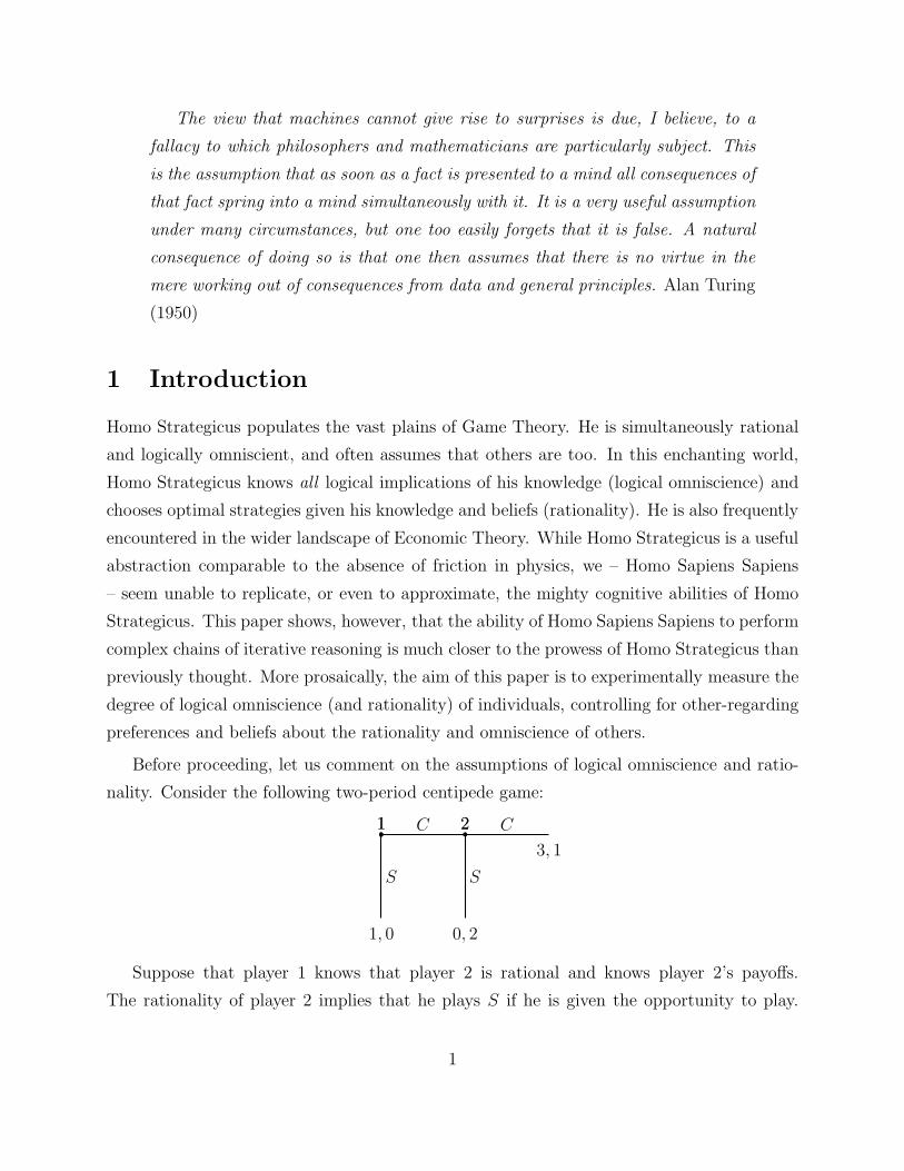
Before proceeding, let us comment on the assumptions of logical omniscience and ratio-

nality. Consider the following two-period centipede game:

S

1, 0

1 C1

S

0, 2

2 C

3, 1

2

Suppose that player 1 knows that player 2 is rational and knows player 2’s payoffs.

The rationality of player 2 implies that he plays S if he is given the opportunity to play.

1

Hence, a logically omniscient player 1 knows that if he plays C, his payoff will be 0, as

player 2 then will play S, while playing S secures a payoff of 1. A rational and logically

omniscient player 1 therefore plays S. Thus, if it is common knowledge that players 1 and 2

are incarnations of Homo Strategicus, it is natural to expect (S, S) to be the strategy profile

which is being played. And, indeed, (S, S) is the unique subgame-perfect equilibrium of this

game. More generally, Aumann (1995) has shown that common knowledge of (substantive)

rationality implies backward induction in dynamic games of perfect information.1 Although

not explicitly stated in Aumann’s formulation, common knowledge of logical omniscience

is fundamental in reaching this conclusion. To see this, suppose that player 1 is not fully

omniscient. He might then fail to infer from his knowledge of player 2’s rationality and payoff

that player 2 would play S if given the opportunity. Nonetheless, he might still be rational,

i.e., play an optimal strategy, e.g., C, given his beliefs about the play of his opponents.

Logical omniscience is conceptually different from rationality. Yet, both logical omniscience

and rationality are hardly distinguishable in practice and, consequently, often jointly referred

to as “rationality” in the literature.2

In an extreme case, the real-world might be entirely populated by Homo Strategicus and

yet real-life behavior might deviate from equilibrium predictions. The fact that all individu-

als involved in strategic interaction are logically omniscient and rational does not guarantee

subgame perfection; common knowledge of this fact is required. Additionally, the relevant

payoffs of the game have to be known, where the relevant payoffs are not necessarily iden-

tical to the material payoffs and may include psychological components.3 Consequently, all

experimental attempts to measure the level of logical omniscience and rationality in humans

by analyzing behavior in strategic games require some auxiliary hypotheses on subjects’ per-

1Aumann (1995) distinguishes between “substantive” and “material” rationality. Substantive rationality

stipulates that a player would act rationally at every decision node, even if this player knows that some

of his decision nodes won’t be reached. In contrast, material rationality stipulates that a player would act

rationally only at the decision nodes he knows to be reached. In general, common knowledge of “material”

rationality does not imply backward induction.2Framing effects are another pitfall that Homo Strategicus avoids. If two decision problems, although

framed differently, are logically equivalent, then logically omniscient individuals do recognize their logical

equivalence, and consequently adopt the very same decision in each problem (Lipman (1999)).3To see this, suppose player 1 is logically omniscient and knows that player 2 also is. Furthermore, suppose

that player 1 believes that player 2 has a strong preference for social efficiency and prefers the allocation

(3, 1) over (0, 2). In this case, “off-equilibrium” strategy C is chosen. We refer the reader to Battigalli and

Dufwenberg (forthcoming) for more examples of dynamic psychological games.

2

ception of the cognitive abilities and preferences of others. Bounded rationality and other

factors (strategic uncertainty, social preferences, overconfidence, etc.) cannot be cleanly sep-

arated in such experiments. In this paper, we propose a novel experimental design, which

makes it possible to measure the degree of logical omniscience and rationality of individuals

without confounding factors.

The experiment we designed is a variant of the Red Hat Puzzle (also known as the

Dirty Faces Game), in which we control for other-regarding preferences and beliefs about

the rationality of others. In the Red Hat Puzzle (thereafter RHP), a player has to determine

her type (hat’s color) by the use of iterative reasoning. For this purpose the player can

use her knowledge about the types of the other players and the other players’ actions. The

distribution of types determines how many iteration steps a player has to perform in order

to arrive at the correct answer.4 In its original form (as used by Weber (2001) or Bayer and

Chan (2007)), the RHP suffers from the same problems as other interactive games when

used to measure the iteration ability in the laboratory. Players have to rely on the iterative

abilities of other players and, therefore, not only their own iterative ability matters but also

their beliefs about the ability of others, beliefs about beliefs about the ability of others, etc.

Social preferences might also play a role. To overcome this problem we do the following:

we transform the RHP into an interactive decision problem where every “player” at each

move has a unique logically correct answer. In each game, a single human player plays with

computer players only.5 The computer players are programmed to be logically omniscient,

i.e. they always choose the logically correct answer. This fact is communicated to the

human player. In this setup a human player, who is able to perform the necessary number of

iteration steps for a particular puzzle, can fully rely on the other players’ logical omniscience.

Additionally, we do not have to worry about the influence of social preferences as the human

player does not interact with other humans. Although similar to a simple decision problem,

our procedure is not: computer-players do interact with the human-subjects in that their

“actions” will depend on the action of the human subjects, and reciprocally. With this

procedure, we can cleanly isolate and measure the iteration ability of humans in an interactive

situation by varying the type distribution within a subject.

Our experiment highlights two interesting patterns. Firstly, subjects were able to per-

4A detailed description of the puzzle will be given below.5For others experimental designs with automated opponents, see Johnson et al. (2002) and McKinney

and Van Huyck (2007).

3

form about two to three steps of iterative reasoning on average, more than the one to two

steps typically measured in games without control for beliefs about the rationality of others.

This result masks a more subtle pattern, however. Subjects solving puzzles requiring three

iterations were also able to solve puzzles requiring more iterations, while many other sub-

jects failed at puzzles requiring two iterations and, consequently, were not able to solve the

puzzles requiring more steps. In other words: The ability to solve puzzles requiring one or

two steps of iteration does not predict the ability of solving puzzles requiring three or four

steps, while solving puzzles requiring three steps does. Our experiment thus suggests what

one could call the slippery slope of logical omniscience. A second result refers to learning:

to our surprise, subjects did not only learn from observation (feedback). Introspection alone

was sufficient for subjects to perform better when playing the same puzzles for a second

time.6 Our econometric analysis is organized around these two themes (Section 4).

This paper contributes to the large literature on iterative reasoning in games e.g., McK-

elvey and Palfrey (1992), Beard and Beil (1994), Nagel (1995), Ho, Camerer and Weigelt

(1998), Goeree and Holt (2001), Van Huck, Wildenthal and Battalio (2002), Cabrera, Capra

and Gomez (2006), to name just a few.7 A recurring feature of many of these studies is

the use of games solvable by iterated deletion of strictly or weakly dominated strategies.8

In these studies, the ability of individuals to perform iterative reasoning is associated with

their ability to iteratively delete dominated strategies. Centipede games (e.g., McKelvey and

Palfrey (1992)) and beauty contest games (introduced to the literature by Nagel (1995)) are

two of the most commonly used games in that literature. However, in those games, iterating

to the equilibrium might actually not be optimal for a subject. To see this, re-consider

the centipede game above. If player 1, the first mover, believes that player 2, the second

mover, won’t realize that it is optimal to stop at the first stage, then it might be optimal for

player 1 to choose the “non-equilibrium” action C at the first stage. After all, it is optimal

for player 1 to stop precisely at the stage before the one where he believes player 2 will

stop. Without controlling for beliefs about the rationality and logical omniscience of others,

failure to play the equilibrium cannot be interpreted as limited ability to perform iterated

reasoning.9 Consequently, a researcher interested in the ability of humans to perform chains

6A similar observation is made in Weber (2003).7We refer the reader to chapter 5 of Camerer (2003) for a survey of this literature.8Note that the solution concept of iterated deletion of weakly dominated strategies requires more stringent

conditions than common knowledge of rationality (see Brandenburger et al. (2008)).9The same is true for beauty contests where a logically omniscient player chooses the number corre-

4

of iterative reasoning might underestimate the actual ability of humans when relying on

choices in beauty contest or centipede games alone. The same is true, to our knowledge, for

all studies of interactive games aiming to measure the iteration abilities of humans.10

The studies mentioned above generally conclude that on average individuals behave as if

they are able to perform one to two iterations. Given that individuals – due to the nature

of the problems discussed – do not necessarily have an incentive to reveal their ability, this

conclusion might be too pessimistic.11

Another approach consists in postulating auxiliary assumptions on the behavior and

beliefs (types) of individuals, and to estimating the type distributions from data collected in

experiments (see, among others, Stahl and Wilson (1994, 1995), Costa-Gomes et al. (2001),

Camerer et al. (2004), or Costa-Gomez and Crawford (2006)). For instance, Stahl and

Wilson (1994) postulate the following “behavioral” types. The first type L0 randomizes

uniformly among all his strategies. The second type L1 conjectures that his opponent is of

type L0 and, consequently, best replies to a uniform distribution over all the actions of his

opponents. The third type L2 conjectures that his opponent is of type L1 and, thus, plays a

best-reply to an action of his opponent, which is a best-reply to a uniform distribution over

his own action. In general, a player of type Lk plays a best-reply to the best-reply of a type

L(k − 1).12 A higher k is thus associated with more sophisticated reasoning. However, the

type of an individual is only an imperfect measure of his ability to perform chains of iterative

reasoning. Indeed, a type L2, for instance, might well be able to perform more sophisticated

chains of reasoning, but his conjecture about the play of his opponent implies that he has

to perform only a few iterations of reasoning. Observing a type – say L2 – just means that

the player can at least perform the few iterations needed for L2, but may be able to perform

sponding to one more iteration step than he believes the others are able to perform. Failing to choose the

equilibrium number is not necessarily a sign of limited iterative ability.10Gneezy et al. (2007) and Dufwenberg et al. (2008) use a version of the game “Nim” to study if and

how humans learn backward induction. Since there players have (weakly) dominant strategies, this zero-

sum game can be used to measure the depth of iterative reasoning in humans if one accepts the auxiliary

hypothesis that it is common knowledge that nobody deliberately plays weakly dominated strategies.11Considerable cross-game variation also indicates that the inferred ability might not be accurate. See

Camerer et al. (2004, Tables 2 and 3).12To control for other-regarding preferences, an “altruistic” type, maximizing the sum of payoffs, is often

assumed. However, a wide range of other-regarding preferences (e.g., Fehr and Schmidt (1999) or Charness

and Rabin (2002)) are not accounted for.

5

many more.13

These studies using k-level hierarchies of decision making are very valuable as they pro-

vide us with insights on how humans play in games where they need to have models of the

rationality and omniscience of others. Recent studies of this kind further improve our un-

derstanding of how cognition in specific games takes place by adding more types and either

tracking how individuals gather information (Costa-Gomes et al. (2001)) or eliciting beliefs

of individuals about the actions of others (Costa-Gomes and Weizsacker (2008)) in matrix

games.14 However, estimating k-level models involves joint hypotheses and, therefore, cannot

directly provide information on the iterative abilities of an individual.

This paper follows yet another route. Our primary question is the following. How closely

related is the Homo Sapiens Sapiens to Homo Strategicus with respect to logical omniscience?

Or in other words: how many iterations can humans actually do if we remove all strategic

uncertainty and control for social preferences? The purpose of this approach is two-fold.

First, we want to clarify if humans are actually as limited in their cognitive abilities as

previous studies suggest. Second, we want to provide the tools and results that can be used

to augment the analysis of cognitive decision making in games by providing a measurement

of actual levels of “bounded rationality.” We believe that this is helpful in order to tackle

the question of how much deviation from equilibrium behavior can be attributed to strategic

uncertainty or social preferences and how much to the lack of logical omniscience.15

The remainder of the paper is organized as follows. Section 2 explains the Red Hat

puzzle in detail and highlights the difficulties in implementing it in the laboratory. Section 3

describes our design. Sections 4 and 5 are devoted to our main results. Section 6 concludes.

2 A simple experiment: the Red Hat puzzle

This section presents a simple puzzle, which will be the basis for our experiment. We follow

the exposition of Fagin et al. (1995). Consider N individuals “playing” together. Each of

these individuals has either a red hat or a white hat, observes the hat color of others, but

13Camerer et al (2004) consider more sophisticated conjectures: a player of type of Lk conjectures that

his opponent might be of any type Lk′ with k′ < k with strictly positive probability.14Costa-Gomes and Weizsacker’s results are somewhat unsettling, as they find that subjects’ actions are

not consistent with their (stated) beliefs about the actions of others.15In a companion paper, Bayer and Renou (2009), we use our measure of logical omniscience along with

measures of other-regarding preferences to explain the play of individuals in strategic-form games.

6

cannot observe the color of his own hat. Suppose that some of the individuals, say n > 0,

have a red hat. Along comes a referee, who declares that “at least one player has a red hat

on the head.” The referee then asks the following question: “What is your hat color?” All

players then simultaneously choose an answer out of “I can’t possibly know”, “I have a red

hat”, or “I have a white hat.” Players then learn the answers of the other players and are

asked again what their hat color is. This process is repeated until all players have inferred

their hat color. This problem is known as the Red Hat Puzzle.16

We can prove that the n − 1 first times the referee asks the question, individuals should

answer “I cannot possibly know,” and the n-th time, individuals with red hats should all

answer “I have a red hat.” The proof is by induction on n.17 For n = 1, the single individual

with a red hat sees that no one else has a red hat. Since it is commonly known that there is

at least one red hat, he must conclude that he is the one. Now suppose that n = 2, i.e., there

are two individuals (say 1 and 2) with a red hat. Both should answer “I cannot possibly

know” the first time the question is asked, as both see another red hat. The information

that there is at least one red hat does not help. However, when individual 2 says “I cannot

possibly know,” individual 1 realizes that he must have a red hat. For otherwise, individual

2 would have known that he has a red hat right away and should have answered “I have a

red hat” the first time the question was asked. Thus, individual 1 can infer wearing a red hat

and should answer “I have a red hat” the second time the question is asked (after observing

2’s answer, of course). Similarly, individual 2 must conclude that he has a red hat.

In the next round the other players can infer that they must have white hats. The fact

that the two players with red hats were able to figure out that they are wearing red hats after

observing one round of answers (by the logic above) implies that both of them can only have

seen one red hat each. The remaining players can infer that their hat cannot be red, as they

now know that there are two red hats in total and they see these two red hats on the heads

of others. They answer: “I have a white hat.” This logic naturally extends to situations

with n = 3, 4, ..., N . The greater the number of red hats an individual observes, the more

complex is the reasoning needed to logically infer the color of one’s own hat. An individual

needs m + 1 iteration steps to figure out his hat color, where m denotes the number of red

16The same game is also known as the “Dirty Faces Game.” For an alternative exposition see Fudenberg

and Tirole (1991) or Osborne and Rubinstein (1994).17Equivalently, we can show that an individual correctly infers the color of his hat (red or white) after

m + 1 iterations (questions) if he observes m red hats.

7

hats this individual sees.

It is important to note that the above logic for a player correctly inferring his hat color

does not rely on the assumption of logical omniscience alone. The remainder of this section

examines the additional assumptions necessary and discusses the difficulties arising with

respect to experimental implementation.

Firstly, the logic above rests on the assumption of common knowledge of logical omni-

science. Even if an individual is logically omniscient, he also needs to know that the answers

of the other individuals are logically correct. To see this, suppose that there is a unique red

hat and individual 1 observes this red hat. Individual 1 can only correctly infer his hat color

(white) if the player, who wears the red hat, answers the first question accurately with “I

have a red hat”. It follows that any experimental design using the red-hat puzzle to measure

the human ability of performing iterated chains of reasoning has to make sure that each

individual knows that the answers of other players are logically correct. Otherwise, it would

not be possible to separate the effects of subjects’ cognitive limitations from those caused

by their beliefs about the cognitive abilities of others.

Secondly, the event “There is at least one red hat” must also be common knowledge,

otherwise individuals are not able to infer their hat color. To see this, suppose that there

is only one red hat. The individual with the red hat observes three white hats, but clearly

cannot infer the color of his hat if he does not know that there is at least one red hat.

Moreover, even if he knows that there is at least one red hat, the individuals with the white

hats cannot infer their hat color if they do not know that the individual with the red hat

knows that there is at least one red hat, etc. Our experimental design has therefore to ensure

that the event “There is at least one red hat” is common knowledge.

Thirdly, individuals must have incentives to correctly infer their hat color and to truth-

fully report their logical inferences (even at intermediate steps). Moreover, since an indi-

vidual’s answer influences the subsequent answers of others and, therefore, their payoffs, an

individual might want to manipulate his answers to affect the payoff of others if he has other-

regarding preferences. Our experimental design will need to properly incentivize individuals

and to exclude any confounding influences from social preferences.

As already argued in the introduction, previous experiments measuring the ability of

individuals to perform chains of iterative reasoning have typically used games solvable by

iterated deletion of strictly or weakly dominated strategies (see Camerer (2003), chapter

5). The failure to control for common knowledge in logical omniscience and rationality and

8

social preferences casts a shadow of doubt on previous results. An individual might well be a

perfect incarnation of Homo Strategicus, and yet fail to play “equilibrium” actions. A doubt

about the omniscience and rationality of others is enough to derail the process of iterated

deletion of dominated strategies.

3 Experimental protocol and treatments

This section describes our experimental protocol, and how it addresses the difficulties dis-

cussed in the previous section.

In our experiment, a human subject was paired with three computers, which were acting

as “players.” Pairing an individual with computers has several advantages given our objec-

tive. Firstly, we can reasonably assume that individuals have no concerns for the eventual

“payoffs” of computers. Secondly, we can ensure that a subject knows that the computers’

answers are logically correct by a) programming the computer-players to choose the logically

correct answers and b) communicating this credibly to the subject. Accordingly, computers

were programmed to choose the logically correct answers at each round of questions (see

below), and the instructions emphasized this point heavily.18 Additionally, subjects were

told (and constantly reminded with an on-screen message) that there was at least one red

hat.

Subjects were asked to infer their hat color from the information given to them. At

any point when they were asked, they had three possible answers to choose from: “I have

a WHITE hat with certainty,” “I have a RED hat with certainty,” and “I cannot possibly

know.” The first time a subject had to choose an answer within a puzzle the information a

subject had was the hat color of the three computer-players (along with the fact that there

was at least one red hat). In any subsequent round within the puzzle, the information a

subject had was the complete history of all answers of all players (the computers’ and his)

in all previous rounds. Similarly, the initial information a computer-player had was the hat

color of the two other computers and the human-subject and, subsequently, the complete

history of answers. The computers’ answers at each point where they were asked was the

(unique) logically correct answer inferred from their information and history (assuming that

the human player was logically omniscient). Before subjects started the experiment, they

had to answer some control questions testing their understanding of the instructions and

18Instructions are available at http://www.le.ac.uk/economics/lr78/.

9

screen layout (see Figure 5 in the Appendix).

A RHP was stopped after either a wrong answer by the human or a correct announcement

of the hat color.19 This stopping procedure is necessary to avoid logical inconsistencies.

Suppose there is only one red hat, which is worn by the human subject. The subject initially

observes three white hats. Now, if the subject (wrongly) answers “I cannot possibly know,”

then computers should logically infer and, if allowed, answer “I have a red hat.” However,

this contradicts what the subject observes. Although the computers in this case would chose

the logically correct answer, we would have lost control over how a subject interprets this

inconsistency. We believe that the observation of contradicting computer announcements

and physical reality would have led subjects to believe that the computers were not properly

programmed or that our claim that the computers are logically omniscient was based on

deception. Stopping a RHP puzzle early does not have any negative consequences for our

ability to measure the performance of subjects, as observing the stage where a subject makes

the first mistake in a puzzle contains all the information needed.

Since each individual was paired with three computers, we had seven possible distinct

logical situations. A logical situation was determined by the number of red hats a subject

saw and whether the subject had a red or white hat herself. The more red hats a subject

was observing, the more steps (iterations) were required to correctly infer the hat color. We

took full advantage of these seven situations to measure the degree of logical omniscience

and rationality of individuals.

Treatments. Our experiment consists of six treatments. The treatments differ by the

number and order of puzzles presented to the subject, as well as by the feedback given.

Puzzles could be ordered in increasing order of complexity (i.e. the number of red hats a

subject observed was weakly increasing from one puzzle to the next), or the ordering of

the puzzles could be random. In some treatments subjects got feedback on whether they

solved the previous puzzle correctly or not. In others they did not receive any feedback

about previous success or failure. The idea behind varying feedback and order was two-fold.

Firstly, this allows us to conduct robustness checks on our measure of logical omniscience.

Secondly, we can gain an insight into the conditions under which subjects are able to learn

to perform more complicated chains of reasoning.

In treatments I-IV, subjects were asked to play two series of the seven situations presented

19At a given round, announcing a hat color was correct only if it was actually possible to infer the hat

color at this given round.

10

above. In treatment I, the seven situations were ordered in increasing order of complexity

and feedback was provided after each round. In treatment II, the seven situations were also

ordered in increasing order of complexity, but no feedback was provided. In treatment III,

the seven situations were randomly ordered and feedback was provided. In treatment IV,

the seven situations were randomly ordered and no feedback was provided. In treatment V

(the one-shot treatment), subjects were asked to play one and only one situation, chosen at

random among the seven possible situations. The random draws were independent across

subjects. The objective of this additional treatment was to control for pattern recognition

and learning within a sequence of the seven situations. Lastly, in treatment VI, subjects were

asked to play the seven situations in increasing order of complexity (without feedback) and

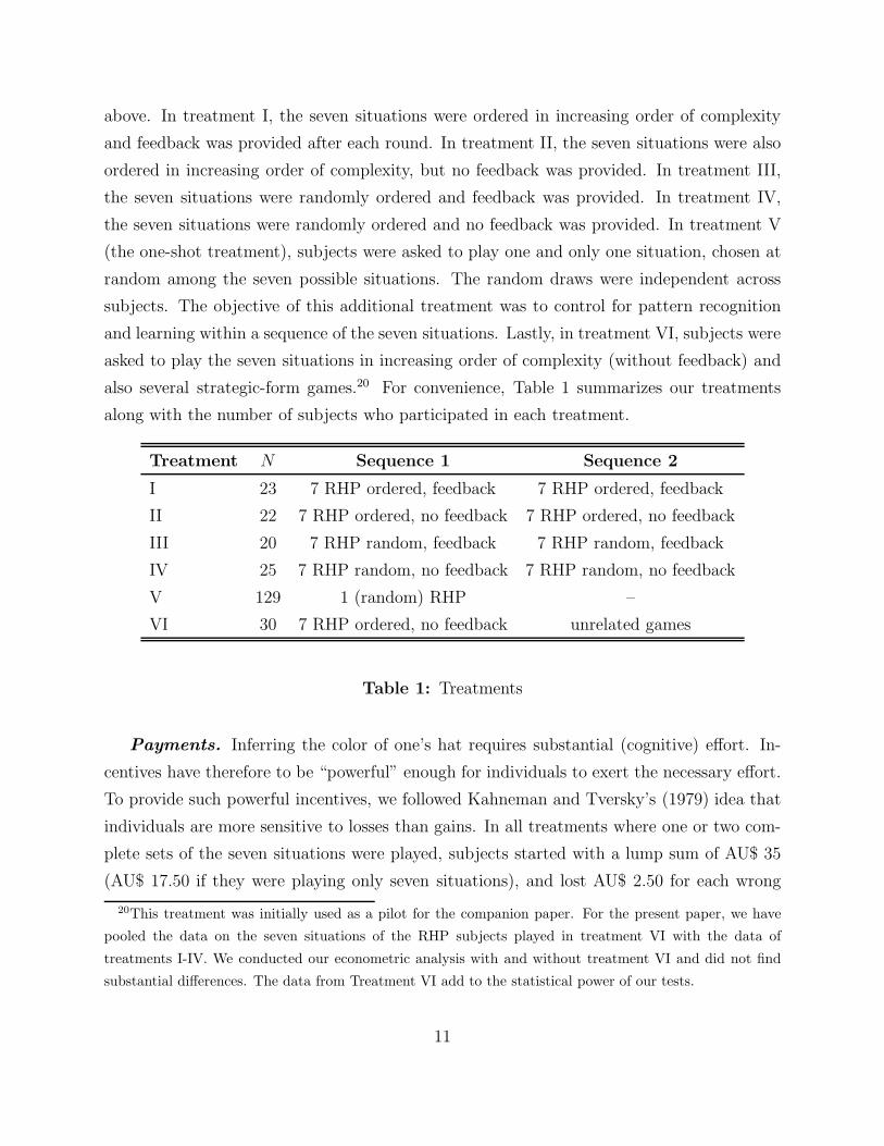
also several strategic-form games.20 For convenience, Table 1 summarizes our treatments

along with the number of subjects who participated in each treatment.

Treatment N Sequence 1 Sequence 2

I 23 7 RHP ordered, feedback 7 RHP ordered, feedback

II 22 7 RHP ordered, no feedback 7 RHP ordered, no feedback

III 20 7 RHP random, feedback 7 RHP random, feedback

IV 25 7 RHP random, no feedback 7 RHP random, no feedback

V 129 1 (random) RHP –

VI 30 7 RHP ordered, no feedback unrelated games

Table 1: Treatments

Payments. Inferring the color of one’s hat requires substantial (cognitive) effort. In-

centives have therefore to be “powerful” enough for individuals to exert the necessary effort.

To provide such powerful incentives, we followed Kahneman and Tversky’s (1979) idea that

individuals are more sensitive to losses than gains. In all treatments where one or two com-

plete sets of the seven situations were played, subjects started with a lump sum of AU$ 35

(AU$ 17.50 if they were playing only seven situations), and lost AU$ 2.50 for each wrong

20This treatment was initially used as a pilot for the companion paper. For the present paper, we have

pooled the data on the seven situations of the RHP subjects played in treatment VI with the data of

treatments I-IV. We conducted our econometric analysis with and without treatment VI and did not find

substantial differences. The data from Treatment VI add to the statistical power of our tests.

11

answer. In treatment V, we used a lottery system, where five winners of substantial prices

(AU$ 300 each) were drawn from the pool of subjects who correctly solved their puzzle. The

average payment was AU$ 24.89 for treatment I, AU$ 19.54 for treatment II, AU$ 21.12 for

treatment III, AU$ 23.3 for treatment IV, AU$ 11.62 for treatment V, and AU$ 8.33 for

treatment VI.21

The experiments took place at AdLab, the Adelaide Laboratory for Experimental Eco-

nomics at the University of Adelaide in Australia. Treatments I-IV took place on 28 August

2005, treatment V took place on 08 June 2006 (two consecutive sessions in parallel labs),

and treatment VI on 05 June 2007. The spreading of the sessions and the parallel session

were designed to prevent information leakage within the subject pool, as solutions to the

RHP can be found on the internet. We used Urs Fischbacher’s (2007) experimental software

Z-tree. The 249 participants were mostly students from the University of Adelaide and the

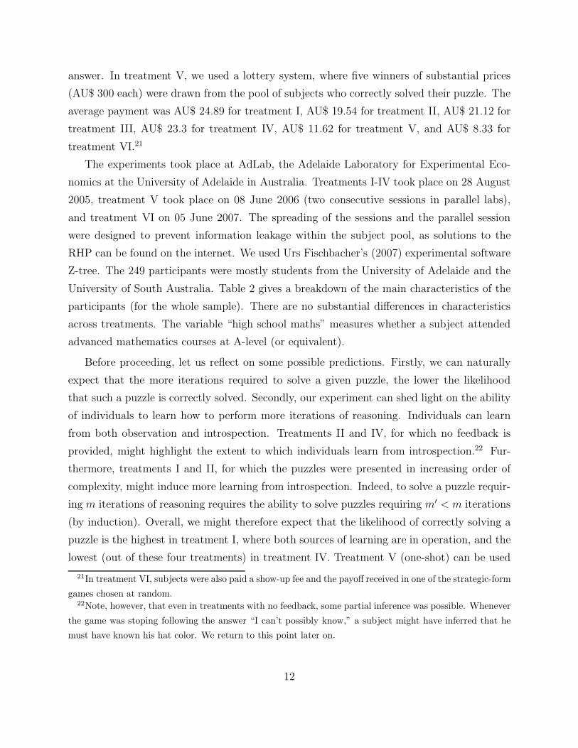
University of South Australia. Table 2 gives a breakdown of the main characteristics of the

participants (for the whole sample). There are no substantial differences in characteristics

across treatments. The variable “high school maths” measures whether a subject attended

advanced mathematics courses at A-level (or equivalent).

Before proceeding, let us reflect on some possible predictions. Firstly, we can naturally

expect that the more iterations required to solve a given puzzle, the lower the likelihood

that such a puzzle is correctly solved. Secondly, our experiment can shed light on the ability

of individuals to learn how to perform more iterations of reasoning. Individuals can learn

from both observation and introspection. Treatments II and IV, for which no feedback is

provided, might highlight the extent to which individuals learn from introspection.22 Fur-

thermore, treatments I and II, for which the puzzles were presented in increasing order of

complexity, might induce more learning from introspection. Indeed, to solve a puzzle requir-

ing m iterations of reasoning requires the ability to solve puzzles requiring m′ < m iterations

(by induction). Overall, we might therefore expect that the likelihood of correctly solving a

puzzle is the highest in treatment I, where both sources of learning are in operation, and the

lowest (out of these four treatments) in treatment IV. Treatment V (one-shot) can be used

21In treatment VI, subjects were also paid a show-up fee and the payoff received in one of the strategic-form

games chosen at random.22Note, however, that even in treatments with no feedback, some partial inference was possible. Whenever

the game was stoping following the answer “I can’t possibly know,” a subject might have inferred that he

must have known his hat color. We return to this point later on.

12

Characteristics Proportion in sample

Gender

male 65.8%

female 34.2%

Courses

arts 3.6%

commerce/finance 38.7%

economics 4.4%

engineering 34.4%

law 2.4%

medicine 8.7%

science 5.5%

other 2.3%

High school maths 76.1%

Age

16-25 91.10%

25-30 6%

31-40 1.1%

> 41 1.8%

Table 2: Demographic characteristics in the sample

(by comparing the success rate to that in the other treatments) to identify learning within

a sequence of RHPs. There no learning is possible. Lastly, we can reasonably conjecture

that almost all individuals can infer that they have a red hat, when initially they do not

observe a red hat (since they were told that there is at least one red hat). Consequently,

correctly solving a puzzle requiring two iterations should have limited predictive power on

the ability to solve puzzles requiring three or four iterations.23 However, correctly solving a

puzzle requiring three iterations should be a better predictor of the ability to perform four

iterations.

23Since solving a puzzle requiring two iterations requires to solve the puzzle requiring one iteration, an

extremely easy task.

13

4 Empirical results

In this section, we first present empirical regularities regarding the likelihood of subjects

correctly inferring their hat color across treatments. We show that the empirical frequency

of correctly solved puzzles is relatively high in all treatments, and certainly much higher than

we expected.24 We will also show that in treatments I-IV, the empirical frequency is much

higher in the second series of seven puzzles than in the first series, and much higher than

in treatment V. This strongly suggests that individuals did learn from introspection and

observation. Furthermore, we will see that the likelihood of solving a puzzle requiring three

and four iterations are about the same, which suggests that individuals able to solve a puzzle

requiring three iterations can also solve puzzles requiring four iterations. Later, we report

the results of our econometric analysis, which confirms the above empirical regularities and

uncovers some other interesting regularities.

4.1 Data analysis

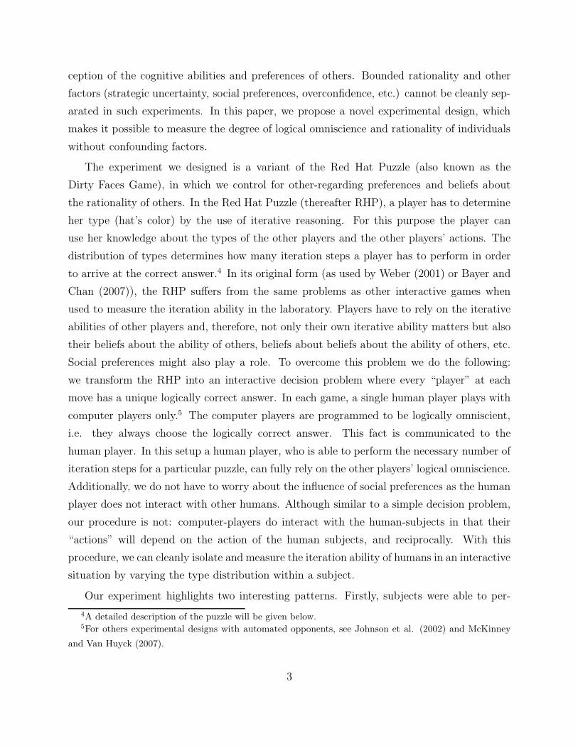
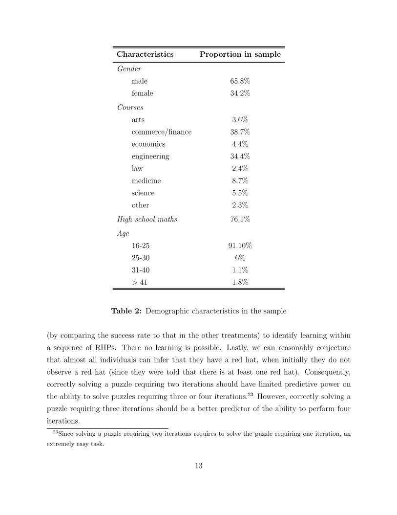
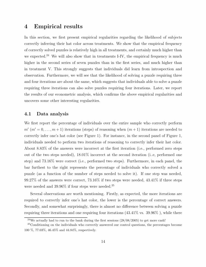
We first report the percentage of individuals over the entire sample who correctly perform

m′ (m′ = 0, . . . , m + 1) iterations (steps) of reasoning when (m + 1) iterations are needed to

correctly infer one’s hat color (see Figure 1). For instance, in the second panel of Figure 1,

individuals needed to perform two iterations of reasoning to correctly infer their hat color.

About 8.83% of the answers were incorrect at the first iteration (i.e., performed zero steps

out of the two steps needed), 18.01% incorrect at the second iteration (i..e, performed one

step) and 73.16% were correct (i.e., performed two steps). Furthermore, in each panel, the

bar furthest to the right represents the percentage of individuals who correctly solved a

puzzle (as a function of the number of steps needed to solve it). If one step was needed,

99.27% of the answers were correct, 73.16% if two steps were needed, 43.41% if three steps

were needed and 39.96% if four steps were needed.25

Several observations are worth mentioning. Firstly, as expected, the more iterations are

required to correctly infer one’s hat color, the lower is the percentage of correct answers.

Secondly, and somewhat surprisingly, there is almost no difference between solving a puzzle

requiring three iterations and one requiring four iterations (43.41% vs. 39.96% ), while there

24We actually had to run to the bank during the first sessions (28/08/2005) to get more cash!25Conditioning on the individuals who correctly answered our control questions, the percentages become

100 %, 77.03%, 46.45% and 44.84%, respectively.

14

050

100

0 1 2 3 4 0 1 2 3 4 0 1 2 3 4 0 1 2 3 4

1 step needed 2 steps needed 3 steps needed 4 steps needed

Per

cent

Frequency of Correct Answers

Figure 1: Frequency of correct answers

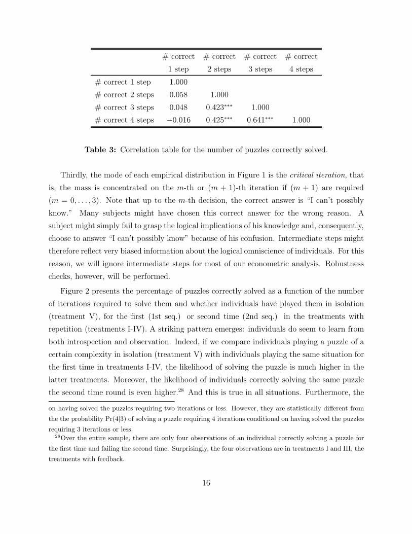
is a significant difference between solving a puzzle requiring two iterations and one requiring

three or four. The pairwise correlations reported in Table 3, reinforce this observation. The

within-subject correlation between the number of correct answers when two and three steps

are required is about the same as the within-subject correlation between the number of

correct answers when two and four steps are required (0.423 vs. 0.425), while the correlation

between the number of correct answers when three and four steps are required is significantly

higher at 0.641.26 This observation suggests that individuals slide down the the slippery slope

of logical omniscience: if an individual can do three steps of iterative reasoning, then she

can do four steps. Our econometric analysis will confirm this empirical observation.27

26Testing for the equality of the correlation coefficients between two and three steps and two and four

steps, we do not reject the null hypothesis, while we do reject the null hypothesis that correlation coefficients

between two and three steps (or two and four steps) and three and four steps are the same.27The probability Pr(m|m′) to correctly solve a puzzle requiring m iterations conditional on having cor-

rectly solved all puzzles requiring up to m′ < m iterations are: Pr(2|1) = .78, Pr(3|1) = .46, Pr(4|1) = .42,

Pr(3|2) = .58, Pr(4|2) = .54, and Pr(4|3) = .8. Again, we have that the probability Pr(3|2) of solving a

puzzle requiring three iterations conditional on having solved the puzzles requiring two iterations or less is

not statistically different from the probability Pr(4|2) of solving a puzzle requiring four iterations conditional

15

# correct # correct # correct # correct

1 step 2 steps 3 steps 4 steps

# correct 1 step 1.000

# correct 2 steps 0.058 1.000

# correct 3 steps 0.048 0.423∗∗∗ 1.000

# correct 4 steps −0.016 0.425∗∗∗ 0.641∗∗∗ 1.000

Table 3: Correlation table for the number of puzzles correctly solved.

Thirdly, the mode of each empirical distribution in Figure 1 is the critical iteration, that

is, the mass is concentrated on the m-th or (m + 1)-th iteration if (m + 1) are required

(m = 0, . . . , 3). Note that up to the m-th decision, the correct answer is “I can’t possibly

know.” Many subjects might have chosen this correct answer for the wrong reason. A

subject might simply fail to grasp the logical implications of his knowledge and, consequently,

choose to answer “I can’t possibly know” because of his confusion. Intermediate steps might

therefore reflect very biased information about the logical omniscience of individuals. For this

reason, we will ignore intermediate steps for most of our econometric analysis. Robustness

checks, however, will be performed.

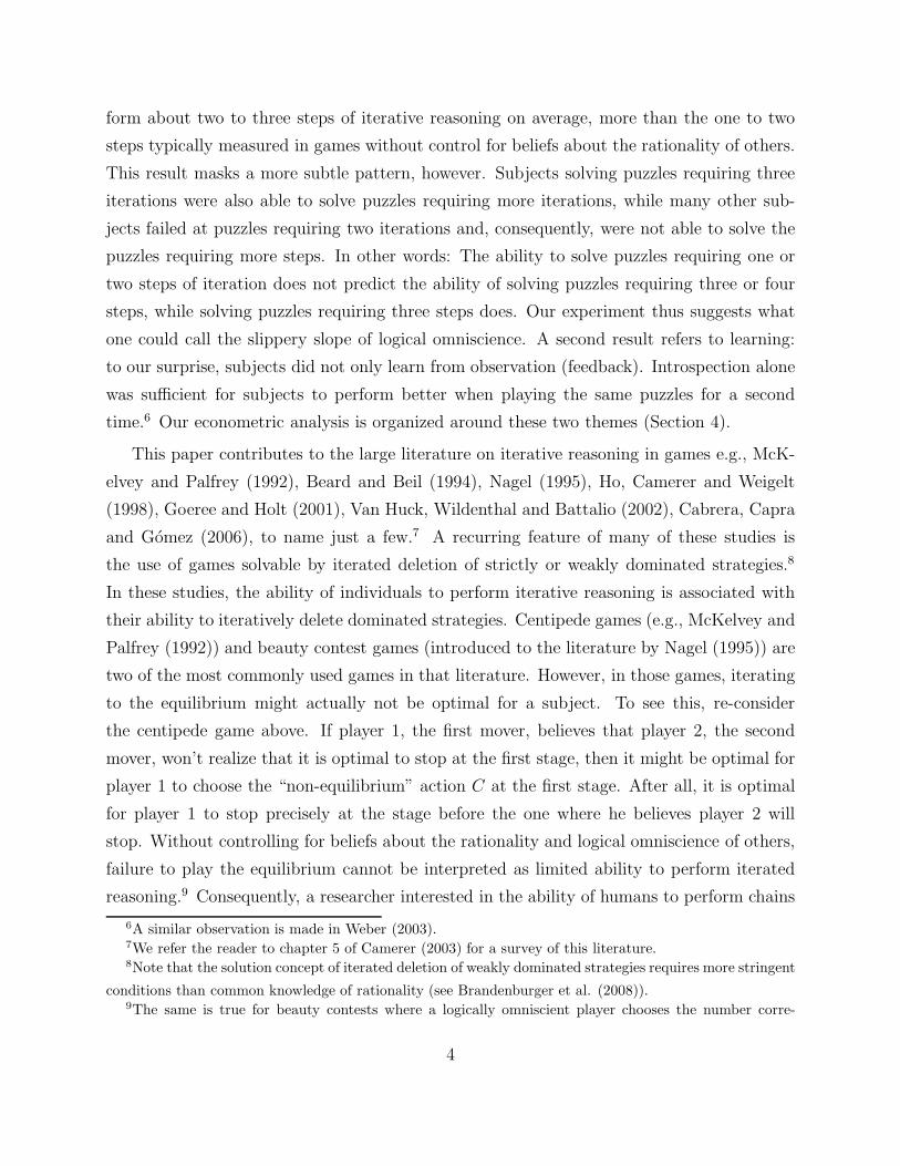
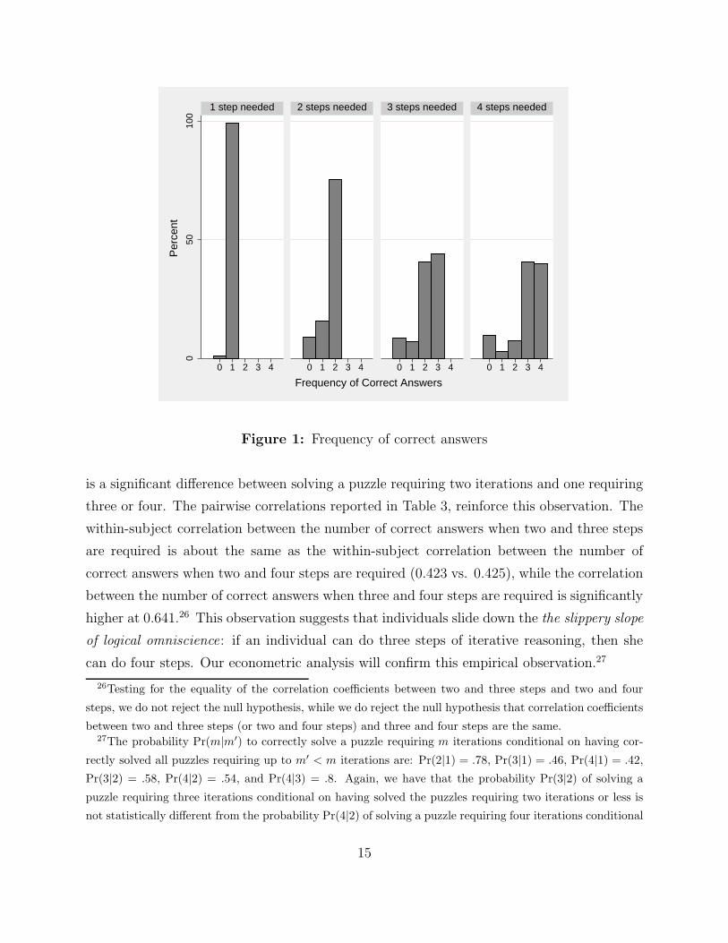
Figure 2 presents the percentage of puzzles correctly solved as a function of the number

of iterations required to solve them and whether individuals have played them in isolation

(treatment V), for the first (1st seq.) or second time (2nd seq.) in the treatments with

repetition (treatments I-IV). A striking pattern emerges: individuals do seem to learn from

both introspection and observation. Indeed, if we compare individuals playing a puzzle of a

certain complexity in isolation (treatment V) with individuals playing the same situation for

the first time in treatments I-IV, the likelihood of solving the puzzle is much higher in the

latter treatments. Moreover, the likelihood of individuals correctly solving the same puzzle

the second time round is even higher.28 And this is true in all situations. Furthermore, the

on having solved the puzzles requiring two iterations or less. However, they are statistically different from

the the probability Pr(4|3) of solving a puzzle requiring 4 iterations conditional on having solved the puzzles

requiring 3 iterations or less.28Over the entire sample, there are only four observations of an individual correctly solving a puzzle for

the first time and failing the second time. Surprisingly, the four observations are in treatments I and III, the

treatments with feedback.

16

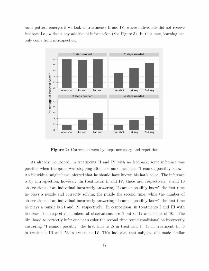
same pattern emerges if we look at treatments II and IV, where individuals did not receive

feedback i.e., without any additional information (See Figure 3). In that case, learning can

only come from introspection.

0.2

.4.6

.81

0.2

.4.6

.81

one−shot 1st seq. 2nd seq. one−shot 1st seq. 2nd seq.

one−shot 1st seq. 2nd seq. one−shot 1st seq. 2nd seq.

1 step needed 2 steps needed

3 steps needed 4 steps needed

Per

cent

age

of P

uzzl

es S

olve

d

Figure 2: Correct answers by steps necessary and repetition

As already mentioned, in treatments II and IV with no feedback, some inference was

possible when the game was stopping after the announcement “I cannot possibly know.”

An individual might have inferred that he should have known his hat’s color. The inference

is by introspection, however. In treatments II and IV, there are, respectively, 9 and 10

observations of an individual incorrectly answering “I cannot possibly know” the first time

he plays a puzzle and correctly solving the puzzle the second time, while the number of

observations of an individual incorrectly answering “I cannot possibly know” the first time

he plays a puzzle is 21 and 19, respectively. In comparison, in treatments I and III with

feedback, the respective numbers of observations are 6 out of 12 and 6 out of 10. The

likelihood to correctly infer one hat’s color the second time round conditional on incorrectly

answering “I cannot possibly” the first time is .5 in treatment I, .43 in treatment II, .6

in treatment III and .53 in treatment IV. This indicates that subjects did made similar

17

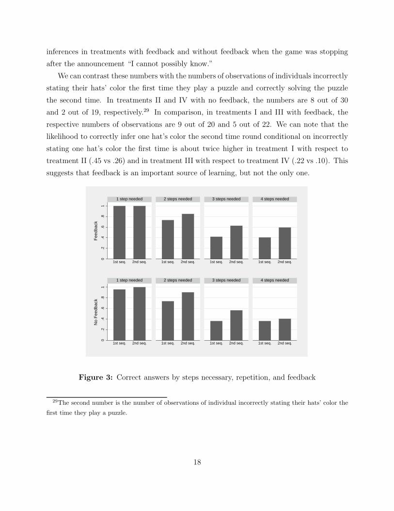
inferences in treatments with feedback and without feedback when the game was stopping

after the announcement “I cannot possibly know.”

We can contrast these numbers with the numbers of observations of individuals incorrectly

stating their hats’ color the first time they play a puzzle and correctly solving the puzzle

the second time. In treatments II and IV with no feedback, the numbers are 8 out of 30

and 2 out of 19, respectively.29 In comparison, in treatments I and III with feedback, the

respective numbers of observations are 9 out of 20 and 5 out of 22. We can note that the

likelihood to correctly infer one hat’s color the second time round conditional on incorrectly

stating one hat’s color the first time is about twice higher in treatment I with respect to

treatment II (.45 vs .26) and in treatment III with respect to treatment IV (.22 vs .10). This

suggests that feedback is an important source of learning, but not the only one.

0.2

.4.6

.81

1st seq. 2nd seq. 1st seq. 2nd seq. 1st seq. 2nd seq. 1st seq. 2nd seq.

1 step needed 2 steps needed 3 steps needed 4 steps needed

Fee

dbac

k

0.2

.4.6

.81

1st seq. 2nd seq. 1st seq. 2nd seq. 1st seq. 2nd seq. 1st seq. 2nd seq.

1 step needed 2 steps needed 3 steps needed 4 steps needed

No

Fee

dbac

k

Figure 3: Correct answers by steps necessary, repetition, and feedback

29The second number is the number of observations of individual incorrectly stating their hats’ color the

first time they play a puzzle.

18

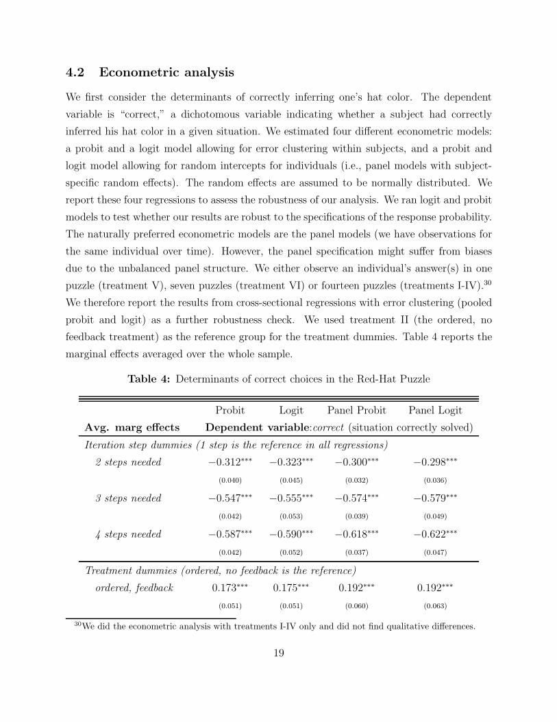
4.2 Econometric analysis

We first consider the determinants of correctly inferring one’s hat color. The dependent

variable is “correct,” a dichotomous variable indicating whether a subject had correctly

inferred his hat color in a given situation. We estimated four different econometric models:

a probit and a logit model allowing for error clustering within subjects, and a probit and

logit model allowing for random intercepts for individuals (i.e., panel models with subject-

specific random effects). The random effects are assumed to be normally distributed. We

report these four regressions to assess the robustness of our analysis. We ran logit and probit

models to test whether our results are robust to the specifications of the response probability.

The naturally preferred econometric models are the panel models (we have observations for

the same individual over time). However, the panel specification might suffer from biases

due to the unbalanced panel structure. We either observe an individual’s answer(s) in one

puzzle (treatment V), seven puzzles (treatment VI) or fourteen puzzles (treatments I-IV).30

We therefore report the results from cross-sectional regressions with error clustering (pooled

probit and logit) as a further robustness check. We used treatment II (the ordered, no

feedback treatment) as the reference group for the treatment dummies. Table 4 reports the

marginal effects averaged over the whole sample.

Table 4: Determinants of correct choices in the Red-Hat Puzzle

Probit Logit Panel Probit Panel Logit

Avg. marg effects Dependent variable:correct (situation correctly solved)

Iteration step dummies (1 step is the reference in all regressions)

2 steps needed −0.312∗∗∗ −0.323∗∗∗ −0.300∗∗∗ −0.298∗∗∗

(0.040) (0.045) (0.032) (0.036)

3 steps needed −0.547∗∗∗ −0.555∗∗∗ −0.574∗∗∗ −0.579∗∗∗

(0.042) (0.053) (0.039) (0.049)

4 steps needed −0.587∗∗∗ −0.590∗∗∗ −0.618∗∗∗ −0.622∗∗∗

(0.042) (0.052) (0.037) (0.047)

Treatment dummies (ordered, no feedback is the reference)

ordered, feedback 0.173∗∗∗ 0.175∗∗∗ 0.192∗∗∗ 0.192∗∗∗

(0.051) (0.051) (0.060) (0.063)

30We did the econometric analysis with treatments I-IV only and did not find qualitative differences.

19

Table 4: . . . continued

Probit Logit Panel Probit Panel Logit

random, feedback 0.092 0.093 0.087 0.087

(0.057) (0.057) (0.070) (0.073)

random, no feedback 0.081 0.084 0.067 0.062

(0.059) (0.058) (0.065) (0.069)

one shot −0.071 −0.075 −0.092 −0.103

(0.049) (0.050) (0.060) (0.062)

Degree dummies (economics is the reference group)

engineering 0.165∗∗ 0.153∗ 0.116 0.113

(0.079) (0.080) (0.103) (0.108)

medicine 0.218∗∗∗ 0.201∗∗∗ 0.178∗ 0.173

(0.079) (0.080) (0.108) (0.107)

Other degrees (arts, commerce, finance, science, law) not significant

gender (male=1) 0.139∗∗∗ 0.142∗∗∗ 0.171∗∗∗ 0.179∗∗∗

(0.040) (0.040) (0.048) (0.051)

control questions OK 0.080 0.079 0.133∗∗ 0.144∗∗

(0.056) (0.057) (0.058) (0.061)

repetition 0.098∗∗∗ 0.093∗∗∗ 0.157∗∗∗ 0.153∗∗∗

(0.023) (0.024) (0.025) (0.025)

time first choice −0.0032∗∗∗ −0.0036∗∗∗ −0.0001 −0.0001

(0.00081) (0.00086) (0.00020) (0.00020)

Dummies for age, advanced math, critical time, all not significant

N 1599 1599 1599 1599

ρ – – 0.504∗∗∗ 0.517∗∗∗

Log-likelihood −745.15 −743.55 −636.97 −630.78

Standard errors in parentheses; *** p <0.01, ** p<0.05, * p<0.1; Prob<χ2<0.0001 (all models)

We organize our econometric analysis around two main themes: iterative reasoning and

learning.

Iterative reasoning. All our regressions confirm our initial observation: the more steps

20

required to solve a puzzle, the less likely it is that an individual solves it (p < 0.01, Wald

tests in all applicable models). For instance, with the Panel Probit model, the probability of

solving a puzzle requiring two steps is 0.3 lower than that for the puzzle requiring one step

(the reference). The probability difference to the one-step puzzle is even lower if three or

four steps are required (lower by 0.574 and 0.618, respectively). Moreover, the likelihood of

correctly inferring one’s hat color when two steps are required is about twice as high as that

for solving a puzzle requiring four steps. This is true for all econometric models. However,

the likelihood does not differ much between three and four steps (e.g., −0.574 vs. −0.618 in

the Panel Probit model). This suggests that individuals who are able to perform three steps

are also able to perform four steps: the slippery slope of logical omniscience. To reinforce

our point, we tested whether solving a puzzle requiring three steps was statistically different

from solving one requiring four steps and could not reject the null hypothesis that they are

equal in any of our four models.31 In contrast, we reject the null hypothesis that solving

a puzzle requiring two steps is equivalent to one requiring three or four steps in all models

(p < 0.01, Wald tests).

Two closely related experimental studies are Weber (2001) and Bayer and Chan (2009).

Weber implements the red hat puzzle as a dynamic game of incomplete information between

two or three human players. Bayer and Chan replicate Weber’s experiment and compare the

replication with a modified version of Weber’s game, where equilibria in weakly dominated

strategies are eliminated.32 As already argued, deviation from equilibrium play cannot be

used to directly estimate the ability of players to do iterative reasoning in those games. Aux-

iliary assumptions such as common knowledge of rationality, common belief in conjectures or

common knowledge of the payoffs (possibly included other-regarding concerns), are required.

By contrast, in our study, the only cause for subjects deviating from the “equilibrium” (i.e.,

the optimal sequence of choices in our decision problem) are their own inability to reason.

Consequently, comparisons between these studies and our study are difficult. The most

severe problem is related to the fact that in the interactive version of the red hat puzzle, a

premature end of the game is possible. All players can end the game at each stage by playing

the action “down,” which is equivalent to choosing the statement “I have a red hat” in our

setting. Whenever a player erroneously (i.e., deviating from the equilibrium path) chooses

31Wald test in all models. The lowest p-value is 0.1725 obtained in the Panel Probit model.32In Weber’s design, a player correctly inferring his hat’s color at stage t was indifferent between revealing

his hat color at stage t or at stage t + 1.

21

this action, the game ends prematurely. Therefore, it is impossible to assess whether the

other players would have played according to the equilibrium strategies in later stages. There

are two reasonable ways of dealing with this problem. Weber implicitly assumes that players,

who had followed the equilibrium path up to the stage where the game ended prematurely,

would have continued on the equilibrium path in later stages. This overestimates equilibrium

agreement. This bias is likely to be large, especially if we consider our findings (see Figure

1) that the last choice a subject has to make is the critical choice and most mistakes are

made at this stage.

A second approach (Bayer and Chan) is to drop all individual observations, where other

players prematurely ended the game. Results based on this second approach are better

suited for comparison with the results of our study, as in our experiment the other players

(the computers) never prematurely end the game. Using this approach, Bayer and Chan

report agreement rates with sequential equilibrium for their three player red-hat game of

86.7 percent when one step of iteration is needed, 10.6 percent when two steps are needed,

and 5.3 percent when three steps are needed. In their modified version of the game, the

agreement is higher (91.7 percent when one step is needed, 39.7 percent when two are and

19.1 percent when three steps are). The success rates in our experiment are thus much higher

than in these studies (see above). This suggests that a high proportion of the deviations

from “equilibrium behavior” observed in the studies of Weber (2001) and Bayer and Chan

(2009) might have resulted from players’ doubts about the rationality of others and not from

their own limited ability.

To assess the robustness of our results, we replicated our econometric analysis treatment-

by-treatment. For treatments II and IV (i.e., the treatments with feedback), signs, coefficient

magnitudes and significance levels of the marginal effects are very similar to the results

obtained for the whole sample. For instance, in treatment II, the likelihood of correctly

inferring one’s hat color is 0.282, 0.568 and 0.611 lower when comparing two, three and

four-step puzzles with the easiest one-step RHP (Panel Probit). Furthermore, as with the

aggregate results, we cannot reject the null hypothesis that solving a puzzle requiring three

steps is equivalent to solving one requiring four steps, while we can reject the null hypothesis

for the comparison between two and three steps and between two and four steps.

For treatments I and III we had to exclude all the observations related to the puzzle

requiring one iteration. In treatments I and III all subjects correctly inferred their hat color

22

when one step was required, creating a problem of hidden collinearity.33 Excluding these

observations and the dummy variable for “1 step needed” we again obtain the result that

solving a puzzle requiring three steps is statistically equivalent to solving a puzzle requiring

four steps, and different from solving a puzzle requiring two steps (the reference step).

However, we can note a difference between treatment I (ordered-feedback) and treatment

III (random-feedback). For treatment I, the likelihood of solving a puzzle requiring three

and four steps is 0.110 and 0.162 lower than for a puzzle requiring two steps, while it is

respectively lower by 0.404 and 0.480 for treatment III. In treatment I, solving a puzzle

requiring three steps was only marginally more difficult than solving one requiring two steps.

This result should be not too disturbing since in treatment I puzzles requiring two iterations

were played first, and feedback was provided (both sources of learning were operating).

Overall, our results are extremely robust.

Learning: feedback and introspection. Table 4 offers two preliminary observations.

Firstly, subjects in treatment I (ordered and feedback) did perform better than subjects in

the reference group (ordered and no feedback); their likelihood of correctly solving a puzzle

is higher by at least 0.17 (p < 0.01, Wald test in all models). In contrast, subjects in the

three other treatments did not perform (statistically) better (coefficients not significant in all

models). Although not significant, subjects in treatment V (one-shot) performed worse than

the reference group. These results seem to suggest that unless an individual benefits from

both sources of learning, i.e., introspection and observation, the likelihood to correctly solve

a puzzle is not affected by learning (no treatment effects). Further econometric analysis

(Table 5) will, however, show that this suggestion is not completely accurate. Secondly,

repetition increases the likelihood of correctly solving a puzzle, with an effect ranging from

0.093 in the Logit model to 0.157 in the Panel Probit model.

To get a deeper understanding of the magnitudes of learning within and across treat-

ments, we ran two additional regressions – a Panel Probit model and a Panel Logit model.

In these regressions, we introduced dummies for treatments and repetition e.g., the dummy

“ordered, feedback, seq. 1” refers to the first sequence of seven puzzles of treatment I. We

used treatment V (the one-shot treatment) as the reference base. These two additional re-

gressions complement our previous regressions in two main respects. Firstly, we decomposed

33More precisely, the covariate pattern “(1 step =1, 2 steps= 3 steps = 4 steps = 0)” only has 1 as

its outcome. Dropping these observations, there is a collinearity problem. For an explanation of hidden

collinearity, we refer the reader to http://www.stata.com/support/faqs/stat/logitcd.html.

23

the marginal effects of a treatment into the marginal effects of a treatment conditional on

whether the first or second sequence of puzzles was played. Due to the very definition of

marginal effects, it is not possible to recover the overall treatment effects from the decom-

posed treatment effects. Secondly, we have changed the reference base to treatment V (the

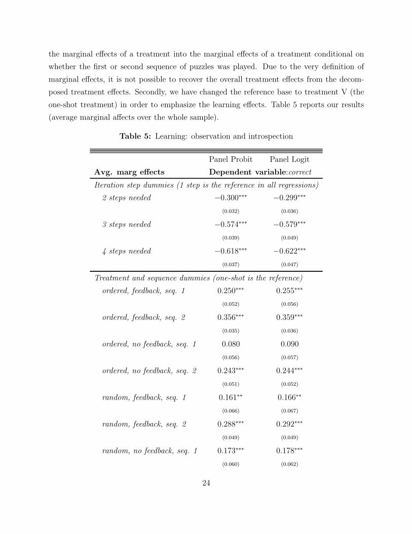
one-shot treatment) in order to emphasize the learning effects. Table 5 reports our results

(average marginal affects over the whole sample).

Table 5: Learning: observation and introspection

Panel Probit Panel Logit

Avg. marg effects Dependent variable:correct

Iteration step dummies (1 step is the reference in all regressions)

2 steps needed −0.300∗∗∗ −0.299∗∗∗

(0.032) (0.036)

3 steps needed −0.574∗∗∗ −0.579∗∗∗

(0.039) (0.049)

4 steps needed −0.618∗∗∗ −0.622∗∗∗

(0.037) (0.047)

Treatment and sequence dummies (one-shot is the reference)

ordered, feedback, seq. 1 0.250∗∗∗ 0.255∗∗∗

(0.052) (0.056)

ordered, feedback, seq. 2 0.356∗∗∗ 0.359∗∗∗

(0.035) (0.036)

ordered, no feedback, seq. 1 0.080 0.090

(0.056) (0.057)

ordered, no feedback, seq. 2 0.243∗∗∗ 0.244∗∗∗

(0.051) (0.052)

random, feedback, seq. 1 0.161∗∗ 0.166∗∗

(0.066) (0.067)

random, feedback, seq. 2 0.288∗∗∗ 0.292∗∗∗

(0.049) (0.049)

random, no feedback, seq. 1 0.173∗∗∗ 0.178∗∗∗

(0.060) (0.062)

24

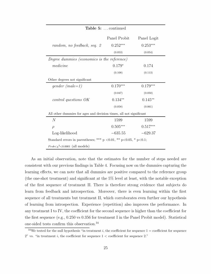
Table 5: . . . continued

Panel Probit Panel Logit

random, no feedback, seq. 2 0.252∗∗∗ 0.253∗∗∗

(0.053) (0.054)

Degree dummies (economics is the reference)

medicine 0.179∗ 0.174

(0.108) (0.113)

Other degrees not significant

gender (male=1) 0.170∗∗∗ 0.179∗∗∗

(0.047) (0.050)

control questions OK 0.134∗∗ 0.145∗∗

(0.058) (0.061)

All other dummies for ages and decision times, all not significant

N 1599 1599

ρ 0.505∗∗∗ 0.517∗∗∗

Log-likelihood −635.55 −629.37

Standard errors in parentheses; *** p <0.01, ** p<0.05, * p<0.1;

Prob<χ2<0.0001 (all models)

As an initial observation, note that the estimates for the number of steps needed are

consistent with our previous findings in Table 4. Focusing now on the dummies capturing the

learning effects, we can note that all dummies are positive compared to the reference group

(the one-shot treatment) and significant at the 5% level at least, with the notable exception

of the first sequence of treatment II. There is therefore strong evidence that subjects do

learn from feedback and introspection. Moreover, there is even learning within the first

sequence of all treatments but treatment II, which corroborates even further our hypothesis

of learning from introspection. Experience (repetition) also improves the performance. In

any treatment I to IV, the coefficient for the second sequence is higher than the coefficient for

the first sequence (e.g., 0.250 vs 0.356 for treatment I in the Panel Probit model). Statistical

one-sided tests confirm this observation.34

34We tested for the null hypothesis “in treatment i, the coefficient for sequence 1 = coefficient for sequence

2” vs. “in treatment i, the coefficient for sequence 1 < coefficient for sequence 2.”

25

We also tested for the magnitude of learning between the two sequences of play across

treatments. More precisely, we tested whether the increase in the likelihood to correctly

solve a given puzzle between the first sequence and the second sequence was the same in

treatment i and treatment j. With two-sided tests, we found no statistical differences in all

treatments but one. The exception is again treatment I (ordered-feedback), which differs

from treatment IV (random-no feedback) at the 10% level.

To summarize, our econometric analysis do suggest that individuals have learned from

both introspection, observation and feedback.

Miscellany. We have also controlled for individual characteristics. The influence of the

degree a subject was studying for is relatively small. Only medical students and, to some

extent, engineering students are performing better than students with other backgrounds.

The marginal effect of training in higher level maths shows the expected sign without being

significant.

We find a surprisingly strong gender effect, however. Depending on the econometric

model, males have a higher probability of correctly inferring their hat color (significant at 1

%-level in all models), with an effect ranging from 0.14 to 0.18. We have no explanation for

this strong gender effect.35

Before the actual decision rounds, we asked subjects two control questions, which show

whether the subjects understood the instructions and the screen layout. As expected, stu-

dents who correctly answered these questions had a higher probability of correctly inferring

their hat color, although this result was not significant in the Logit and Probit models.

Lastly, in our initial regressions, we included the independent variable “Time first choice,”

measuring the time (in seconds) a subject took to make his first announcement in each puz-

zle. In the pooled Probit and Logit models, the time taken for the first announcement

negatively influences the likelihood of solving a puzzle (p < 0.01, Wald test). This variable

proxies unobserved subject-specific characteristics such as intrinsic logical skill, understand-

ing of the presentation of the puzzles, or confidence in their own inferences. Moreover, the

variable “Time first choice” is highly correlated within a subject and across puzzles. How-

ever, allowing for subject-specific random intercepts (the panel models with random effects),

the variable “Time first choice” becomes statistically insignificant, as the unobserved het-

erogeneity in subject-specific characteristics is now absorbed by the random effects. The

35Note, however, that in our companion paper, there is no gender effect, while all other determinants of

correctly inferring one hat’s color are similar.

26

correlation within a subject is now captured by the within-subject correlation coefficient

ρ, which is highly significant and around 0.5 in all our panel models. This indicates that

there is some consistency within subjects: correctly solving a certain puzzle increases the

likelihood of solving another puzzle. The next section investigates whether this consistency

within subjects can be exploited to derive a measure of the degree of logical omniscience.

5 Logical omniscience: a measure

In this section, we construct two simple measures of logical omniscience so as to quantify

the number of steps of iterative reasoning an individual is able to perform.

Each puzzle can be parameterized by a pair (m, n), where m is the number of red hats a

subject observes and n is the actual number of red hats (n = m + 1 or n = m). Remember

that if a subject observes m red hats, m + 1 iterations are required to correctly infer his hat

color: the higher m is, the more complex the chain of reasoning is.

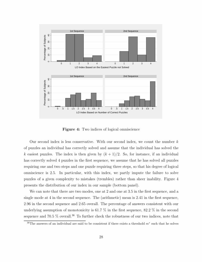
The first index we construct supposes that if an individual can solve a puzzle requiring

m iterations, he must solve all puzzles requiring m′ < m iterations. The degree of logical

omniscience of an individual is then given by the number of iterations required to solve

the most difficult puzzle the individual can solve, conditional on having correctly solved

all puzzles requiring less iterations. So, for instance, if an individual has solved all puzzles

requiring one or two steps of reasoning, but fails to solve a puzzle requiring three steps, his

degree of logical omniscience is two. This index is very conservative, as a subject, who failed

to correctly solve the easiest puzzle, has a degree of 0 regardless of whether he has solved

any (or even all) other puzzles. The first puzzle an individual fails is thus interpreted as the

upper bound on his ability to perform iterative reasoning, regardless of his performance in

the other puzzles. Moreover, this index does not take into account intermediate steps: either

an individual correctly infers the color of his hat or not. Failure to correctly infer one’s hat

color is considered as a complete failure. Figure 4 presents the distribution of our index in

our sample (top panel).

We can note that there are two modes, one at 1 and one at 2 in the first sequence, and a

single mode at 2 in the second sequence. The (arithmetic) mean for our conservative index

is 1.79 in the first sequence, 2.67 in the second sequence, and 2.17 overall. Since the index

gives a lower bound on an individual’s ability, individuals are thus able to perform at least

two iterations of reasoning on average.

27

010

2030

40

0 1 2 3 4 0 1 2 3 4

1st Sequence 2nd Sequence

Per

cent

age

of S

ubje

cts

LO Index Based on the Easiest Puzzle not Solved

010

2030

40

0 .5 1 1.5 2 2.5 3 3.5 4 0 .5 1 1.5 2 2.5 3 3.5 4

1st Sequence 2nd Sequence

Per

cent

age

of S

ubje

cts

LO Index Based on Number of Correct Puzzles

Figure 4: Two indices of logical omniscience

Our second index is less conservative. With our second index, we count the number k

of puzzles an individual has correctly solved and assume that the individual has solved the

k easiest puzzles. The index is then given by (k + 1)/2. So, for instance, if an individual

has correctly solved 4 puzzles in the first sequence, we assume that he has solved all puzzles

requiring one and two steps and one puzzle requiring three steps, so that his degree of logical

omniscience is 2.5. In particular, with this index, we partly impute the failure to solve

puzzles of a given complexity to mistakes (trembles) rather than sheer inability. Figure 4

presents the distribution of our index in our sample (bottom panel).

We can note that there are two modes, one at 2 and one at 3.5 in the first sequence, and a

single mode at 4 in the second sequence. The (arithmetic) mean is 2.41 in the first sequence,

2.96 in the second sequence and 2.65 overall. The percentage of answers consistent with our

underlying assumption of monotonicity is 61.7 % in the first sequence, 82.2 % in the second

sequence and 70.5 % overall.36 To further check the robustness of our two indices, note that

36The answers of an individual are said to be consistent if there exists a threshold m∗ such that he solves

28

the Spearman correlation coefficient of our two indices is 0.8519 with p < 0.0001. The two

indices are highly correlated.

Although it is hard to compare our results with the existing literature on iterative rea-

soning in games (see chapter 5 of Camerer (2003) for a survey), our experiment suggests

that individuals are able to perform more iterations than previously thought. In previous

studies between one and two steps seemed to be the norm (see Nagel (1995), Figure 2, p

1317 for an example). Controlling for preferences and beliefs about the rationality of others

therefore turns out to be important. (See our previous discussion.)

6 Conclusion

Logical omniscience is the ability to draw all logical conclusions from one’s knowledge. For

instance, if a logically omniscient individual knows that his opponents are rational and knows

that they know that he is rational, then he infers that his opponents will not play strictly

dominated strategies. Logically omniscient and rational individuals are the ideal of Game

Theory: the Homo Strategicus. To measure the extent to which individuals are rational

and logically omniscient, this paper designed an experiment, a variant of the Red Hat puz-

zle, controlling for other-regarding preferences and beliefs about the rationality of others.

Controlling for other-regarding preferences and beliefs about the rationality of others is es-

sential. Failure to properly control for those confounding factors might otherwise lead to

underestimating the real ability of individuals. Our index measuring the ability of individ-

uals to perform iterations of reasoning show that individuals can perform more iterations

than previously thought. Moreover, individuals did learn how to perform more iterations of

reasoning from both introspection and feedback.

We believe that our measure of logical omniscience together with measures of other-

regarding preferences might prove extremely useful in explaining deviations from equilibrium

behavior in games. Preliminary results from another study (Bayer and Renou, 2008) suggest

that uncertainty about the rationality and omniscience of others is a key determinant for

why people deviate from equilibrium play. This observation seems to confirm earlier results

reported in Stahl and Wilson (1995) and Costa-Gomez et al. (2001).

all puzzles requiring m ≤ m∗ iterations, and fails all other puzzles.

29

References

[1] Robert J. Aumann (1995), Backward Induction and Common Knowledge of Rationality,

Games and Economic Behavior 8, 6-19.

[2] Pierpaolo Battigalli and Martin Dufwenberg (2009), Dynamic Psychological Games,

Journal of Economic Theory 144, 1-35.

[3] Ralph-C Bayer and Mickey Chan (2007), The Dirty Faces Game Revisited, School of

Economics Working Paper, The University of Adelaide.

[4] Ralph-C Bayer and Ludovic Renou (2009), Departure from Nash Equilibrium: Bounded

Rationality or Other-regarding Preferences. A Controlled Experiment, Mimeo, Univer-

sity of Leicester.

[5] Randolph T. Beard and Richard Beil (1994), Do People Rely on the Self-interested

Maximization of Others? An Experimental Test, Management Science, 40, 252-262.

[6] Adam Brandenburger, Amanda Friedenberg and H. Jerome Keisler (2008), Admissibility

in Games, Econometrica, 76, 307-352.

[7] Susana Cabrera, C. Monica Capra and Rosarie Gomez (2006), Behavior in One-shot

Traveler’s Dilemma Games: Model and Experiment with Advise, Spanish Economic

Review, 9(2), 129-152.

[8] Colin F. Camerer, Teck-Hua Ho and Juin-Kuan Chong (2004), A Cognitive Hierarchy

Model of Games, Quarterly Journal of Economics 119, 861-898

[9] Colin F. Camerer (2003), Behavioral Game Theory: Experiments in Strategic Interac-

tion, Princeton University Press, Princeton, USA.

[10] Gary Charness and Matthew Rabin (2002), Understanding Social Preferences with Sim-

ple Tests, Quarterly Journal of Economics 117, 817-869.

[11] Miguel A. Costa-Gomes, Vincent P. Crawford and Bruno Broseta (2001), Cognition and

Behavior in Normal-Form Games: An Experimental Study, Econometrica 69, 1193-1235.

30

[12] Miguel A. Costa-Gomes and Vincent P. Crawford (2006),Cognition and Behavior in

Two-Person Guessing Games: an Experimental Study, American Economic Review 96,

1737-1768

[13] Miguel A. Costa-Gomes and Georg Weizsacker (2008), Stated Beliefs and Play in

Normal-Form Games, Review of Economic Studies 75, 729-762.

[14] Martin Dufwenberg, Ramya Sundaram and David Butler (2008), Epiphany in the Game

of 21, mimeo.

[15] Uri Gneezy, Aldo Rustichini and Alexander Vostroknutov (2007), I’ll Cross That Bridge

When Come to It: Backward Induction as a Cognitive Process, mimeo.

[16] Ronald Fagin, Joseph Y. Halpern, Yoram Moses and Moshe Y. Vardi (1995), Reasoning

about Knowledge, MIT Press, Cambridge, USA.

[17] Ernst Fehr and Klaus Schmidt (1999), A Therory of Fairness, Competition, and Coop-

eration, Quarterly Journal of Economics 114, 817-868.

[18] Urs Fischbacher (2007), z-Tree: Zurich Toolbox for Ready-made Economic Experiments,

Experimental Economics 10(2), 171-178.

[19] Drew Fudenberg and Jean Tirole (1991), Game Theory, MIT Press, Cambridge, USA.

[20] Jacob K. Goeree and Charles A. Holt (2001), Ten Little Treasures of Game Theory and

Ten Intuitive Contradictions, American Economic Review 91, 1402-1422.

[21] Eric J. Johnson, Colin Camerer, Sankar Sen, Talia Rymon (2002), Detecting Failures of

Backward Induction: Monitoring Information Search in Sequential Bargaining, Journal

of Economic Theory 104, 16-47.

[22] Teck Ho, Colin F. Camerer and Keith Weigelt (1998), Iterated Dominance and Iterated

best-response in Experimental p-beauty Contests, American Economic Review, 88, 947-

969.

[23] Daniel Kahneman and Amos Tversky, (1979), Prospect Theory : An Analysis of Deci-

sion under Risk, Econometrica 47, 263-291.

31

[24] Bart Lipman (1999), Decision without Logical Omniscience: Toward an Axiomatic

Framework for Bounded Rationality, Review of Economic Studies 66, 339-361.

[25] Richard D. McKelvey and Thomas R. Palfrey (1992), An Experimental Study of the

Centipede Game, Econometrica 58, 1321-1339.

[26] C. Nicholas Mc Kinney and John Van Huyck (2007), Estimating Bounded Rationality

and Pricing Performance Uncertainty, Journal of Economic Organization and Behavior

62, 625-639.

[27] Rosemarie Nagel (1995), Unraveling in Guessing Games: An Experimental Study, Amer-

ican Economic Review 85, 1313-1326.

[28] Martin J. Osborne and Ariel Rubinstein (1994), A Course in Game Theory, MIT Press,

Cambridge, USA.

[29] Dale O. Stahl and Paul W. Wilson (1994), Experimental Evidence on Players’ Models

of Other Players, Journal of Economic Behavior & Organization 25, 309-327.

[30] Dale O. Stahl and Paul W. Wilson (1995), On Players’ Models of Other Players: Theory

and Experimental Evidence, Games and Economic Behavior 10, 218-254.

[31] Alan Turing (1950), Computing Machinery and Intelligence, Mind 49, 433-460.

[32] John B. Van Huck, John Wildenthal and Raymond C. Battalio (2002), Tacit Coopera-

tion, Strategic Uncertainty, and Coordination Failure: Evidence from Repeated Domi-

nance Solvable Games, Games and Economic Behavior 38, 156-175.

[33] Roberto A. Weber (2001), Behavior and Learning in the Dirty Faces Game, Experimen-

tal Economics 4, 229-242.

[34] Roberto A. Weber (2003), ‘Learning with No Feedback in a Competitive Guessing Game,

Games and Economic Behavior, 44, 134-144.

7 Appendix

32

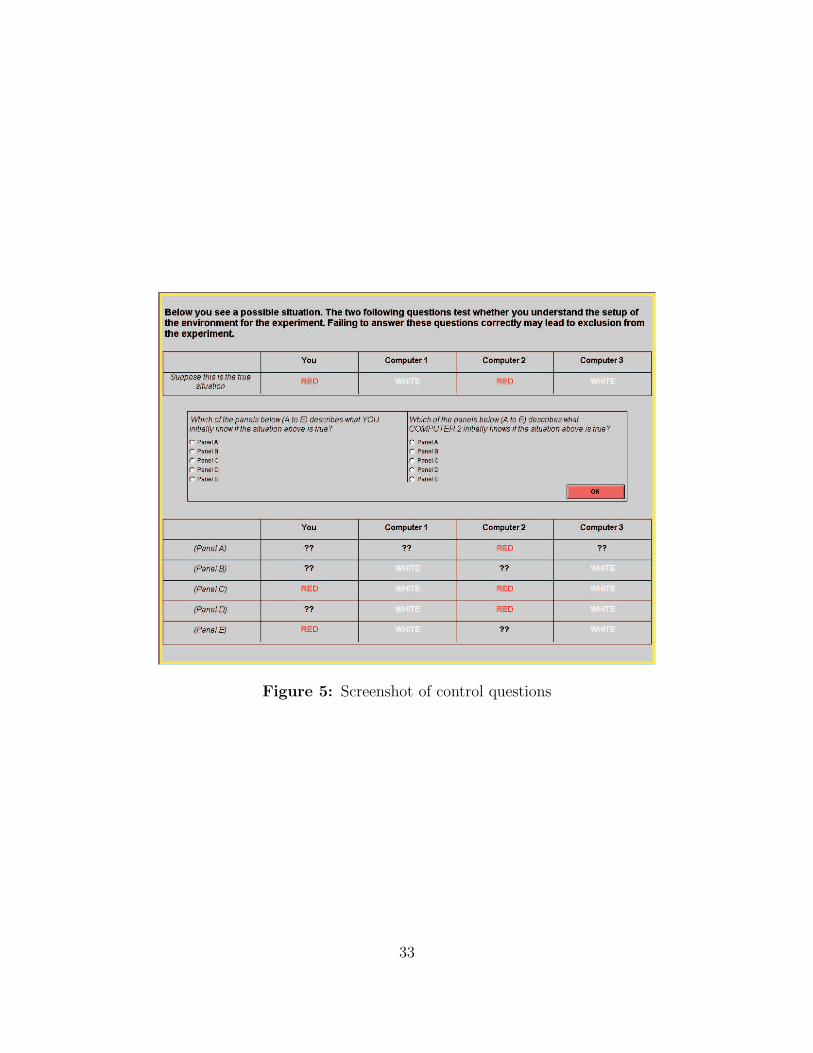
Figure 5: Screenshot of control questions

33

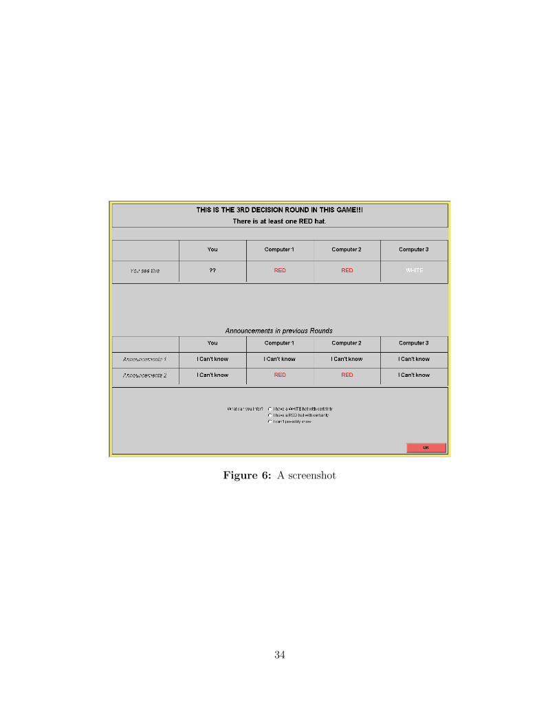
Figure 6: A screenshot

34