1

LONG RANGE FORECASTING OF COLORADO

STREAMFLOWS BASED ON HYDROLOGIC, ATMOSPHERIC,

AND OCEANIC DATA

by

Jose D. Salas and Chongjin Fu

Department of Civil and Environmental Engineering

Colorado State University, Fort Collins, CO

and

Balaji Rajagopalan

Department of Civil and Architectural Engineering

University of Colorado, Boulder, CO

2

ABSTRACT

Climatic fluctuations have profound effects on water resources variability in the western United

States. The effects are manifested in several ways and scales particularly in the occurrence,

frequency, and magnitude of extreme events. The research reported herein centers on streamflow

predictability at the medium and long range scales in the headwaters of six rivers that originate in

the State of Colorado. Specifically, we want to improve the capability of forecasting seasonal

and yearly flows. The analysis will focus on forecasting seasonal (April-July) and yearly (April-

March) and (October-September) streamflows based on atmospheric-oceanic forcing factors,

such as geopotential height, wind, and sea surface temperature (SST), as well as hydrologic

factors such as snow water equivalent (SWE). The approach followed in the study includes:

search for potential predictors, apply Principal Component Analysis (PCA) and multiple linear

regression (MLR) for forecasting at individual sites, apply Canonical Correlation Analysis

(CCA) for forecasting at multiple sites, and test the forecasting models. The forecast models

have been tested in two modes: (a) fitting and (b) evaluation. In addition, some measures of

forecast skill have been utilized. The study includes comparisons of forecasts using all possible

predictors, i.e. hydrologic, atmospheric, and oceanic variables, using atmospheric and oceanic

variables only, and using oceanic predictors only. In addition, we compared forecasts at the six

sites by using aggregation and disaggregation procedures. The study brought into relevance the

significant benefits of using atmospheric and oceanic predictors, in addition to hydrological

predictors, for long range streamflow forecasting. It has been shown that forecasts based on

PCA applied to individual sites give very good results based on various forecast performance

measures for both seasonal as well as yearly time scales. Also it has been shown that even

though the PCA has been applied on a site by site basis yet the forecasts approximate well the

historical cross-correlation although some underestimation was noted for two sites. We also

found that forecasts made using CCA are less efficient than those based on PCA even regarding

the cross-correlations among sites. Furthermore, the forecast procedures based on aggregation

and disaggregation (in the case of multiple sites) produced only modest results.

Keywords: Forecasting streamflows, atmospheric/oceanic predictors, flow prediction,

stochastic analysis, PCA, CCA.

3

Long Range Forecasting of Colorado Streamflows Based on

Hydrologic, Atmospheric, and Oceanic Data

1. Introduction

Although the State of Colorado is located in a semiarid climate it has important water

resources because of its high elevation and significant amount of snowfall every year. Several

major rivers originate in the State of Colorado, such as the Colorado River, Arkansas River, Rio

Grande and others. Agriculture, municipal water supply, hydropower generation, and

recreational activities from the headwater regions down heavily rely on the river waters. Such

water demand has been increasing as the western U.S. continues developing and the population

growing. Thus balancing a limited and variable water supply and competing increasing water

demands must be tackled by water resources management so as to make sufficient amount of

water available at the time is needed. It is a critical aspect of conservation, development, and

management of water resources systems particularly in Colorado because of its semiarid climate.

However, water availability may be severely impacted because of extreme hydroclimatic events

such as droughts. Understanding the variability of such phenomena, particularly determining

their predictability are the main focus of the research reported herein.

There is growing evidence of the effects of atmospheric-oceanic features on the

hydrology of the western basins. Quantifying such effects in the headwaters of Colorado rivers

is difficult because of the varied topography in the Rocky Mountains and because the headwater’

rivers lie outside the regions most strongly influenced by large scale climatic forcing such as

ENSO. The rivers that originate in the State of Colorado and flow downstream across semiarid

and arid lands are prone to frequent and often long periods of low flows. Being important

sources of water supply for many users, they have been developed and controlled with many

river diversions and dams along the system. Operating such systems requires reliable streamflow

forecasts. Every year management decisions for operating the systems are made early in the year

in anticipation of the forthcoming spring and summer streamflows. Thus long range streamflow

forecasting may be of particular interest for improving system operations.

Colorado is a mountainous region and a major source of the streamflows is melting snow.

Therefore snowfall in the preceding months of the season of interest must be an important factor

for streamflow forecasting. However, there are several other factors that affect the fluctuations of

4

the streamflows such as the water content in the atmosphere and its transportation to the area.

For example, Geopotential Height (GH) is a direct indicator of the conditions leading to

precipitation, which could eventually be turned into streamflow. Other variables that could be

used as predictors for streamflow forecasting are air temperature, humidity, and wind.

Temperature and humidity are very much related to the amount of moisture in the air and wind is

an important predictor since it is a determinant factor for moisture transport in the atmosphere.

Also as the oceans are the largest water resources of moisture on earth, ocean dynamics play a

significant role of streamflow variability. Perhaps the most important variable representing

oceanic conditions is sea surface temperature (SST) and many oceanic climatic indices have

been developed such as the Southern Oscillation Index (SOI) and the Pacific Decadal Oscillation

(PDO) index. Since streamflow is a part of the global hydrological circulation, and the changes

of the atmospheric and oceanic conditions certainly affect the variations of streamflows, forecast

models of Colorado rivers must include key atmospheric and oceanic variables as predictors in

addition to snow water equivalent and other hydrological variables that may be of relevance for

the system at hand.

The scope of the study herein centers on streamflow predictability at the medium range

and long range scales in the headwaters of the rivers that originate in the State of Colorado. The

specific objective of the study is to develop and assess models and methods for forecasting

seasonal (April-July) and yearly (April-March and October-September) streamflows for the

Yampa, Gunnison, San Juan, Poudre, Arkansas, and Rio Grande rivers. The models will include

forecasting at single and multiple sites. The forecasts will be based on identifying hydrologic

predictors such as snow water equivalent and predictors from various atmospheric-oceanic

forcing factors such as, geopotential height, zonal and meridional wind, air temperature,

precipitation, sea surface temperature (SST), and streamflows in the study area.

2. Brief Review of Related Studies

Existing medium and long range streamflow forecasting models for Colorado River

basins commonly rely on previous records of snow water equivalent, precipitation, and

streamflows as predictors. And the typical model has been the well known multiple linear

regression. Haltiner and Salas (1988) and Wang and Salas (1991) in studies of the Rio Grande

basin have shown that significant improvements in forecasting efficiency can be achieved using

time series analysis techniques such as transfer function models. Also recent literature have

5

demonstrated the significant relationships between climatic signals such as SST, ENSO, PDO,

and others on precipitation and streamflow variations (e.g. Cayan and Webb, 1992; Mantua et al,

1997; Clark et al, 2001) and that seasonal and longer-term streamflow forecasts can be improved

by using such climatic factors (e.g. Hamlet and Lettenmaier, 1999; Clark et al, 2001; Eldaw et al,

2003; Grantz et al, 2005; Salas et al, 2005). Thus the literature suggests that it is worthwhile

examining in closer detail forecasting schemes that incorporate not only the usual predictors (e.g.

snow water equivalent, precipitation, and streamflows,) but also climatic factors that may

improve the seasonal and long range forecasts of streamflows in the headwaters of Colorado.

Also, previous studies suggested that despite the influence of major climatic factors such as

ENSO on the hydrology of the Colorado basin, there are significant differences in their effects

from basin to basin (McCabe and Dettinger, 2002). This is the reason why in our research we

considered three major streams in the Colorado headwaters (Yampa, Gunnison, and San Juan)

and three other rivers flowing in other directions such as the Poudre, Arkansas, and Rio Grande

rivers.

Therefore, in addition to the typical indices such as ENSO as mentioned before, we

considered predictors directly identified from sea surface temperature, and other atmospheric

circulation features such as geopotential heights (e.g. 700 mb) and zonal meridional winds.

Many studies have pointed out the strong connection between the extreme phases of the El Niño

Southern Oscillation (ENSO) episodes and fluctuations of precipitation and streamflow all over

the world (e.g. Ropelewski and Halpert, 1987; Cayan et al, 1998). For example significant

relationship was found between El Niño and extreme drought years in the Pacific northwest and

a strong relationship between dry conditions in the southern United States and La Niña events

(e.g. Piechota and Dracup, 1996). Also during El Niño above normal precipitation was found in

the desert Southwest (e.g. Cayan and Webb, 1992; Dettinger et al, 1998). Higgins et al (2000) in

forecasting studies of precipitation and surface air temperature in the U.S. based on ENSO, SST,

tropical precipitation, geopotential height, winds and AO found that the dominant factors are

tropical precipitation and AO. Also ENSO influences have been observed on snow water

equivalent (Clark et al, 2001) and streamflows (e.g. Piechota et al, 1997; Maurer et al, 2003). In

studying the Mississippi River basin Maurer et al (2003) found that in the eastern part of the

basin ENSO and AO indices are more important than the land surface stage indicators such as

soil moisture and snow. They also claimed that for 3 months or greater lead times the effects of

6

ENSO and AO are more significant. And Maurer et al (2004) studied the predictability of

seasonal runoff in the Continental U.S. between 25° and 53° N as a function of NAO, AO, NP,

PNA, AMO, Niño3.4, and PDO. For example, they found that a positive phase of El Niño 3.4 is

useful for forecasting the MAM runoff while a negative phase Niño 3.4 is useful for forecasting

the DJF runoff. In addition, effects on decadal time scales primarily driven by the Pacific

Decadal Oscillation (PDO) have been found (e.g. Mantua et al, 1997; McCabe and Dettinger,

1999; McCabe et al, 2004).

Furthermore, Moss et al (1994) used the Southern Oscillation Index (SOI) as a predictor

of the probability of low flows in New Zealand. Eltahir (1996) showed that up to 25% of the

natural variability of the Nile River annual flows is associated with ENSO events and Eldaw et al

(2003) reported that SST in the Pacific and Atlantic oceans in conjunction with precipitation at

the Gulf of Guinea may be used as predictors for forecasting the total streamflows in the Blue

Nile River several months in advance. In addition, Salas et al (2005) in studying the

predictability of droughts in the Poudre River utilized SSTs in the Pacific to forecast the next

years’ flows that may occur in the basin. Also Grantz et al (2005) developed a forecast model

using SST, GH, and SWE as predictors for forecasting April-July streamflows at the Truckee and

Carson rivers in Nevada. They found that forecast skills are significant for up to 5 months lead

time based on SST and GH. Regonda et al (2006) reported successful results for forecasting

streamflows in the Gunnison River using various climatic forcing factors. Maity and Kumar

(2008) developed a forecasting model for monthly streamflows in India based on ENSO and

climatic index of the tropical Indian Ocean. Also in a study of 639 U.S. rivers Tootle et al

(2005) found significant relationships between the ENSO, PDO, AMO, and NAO indices and

streamflows, and suggested that their findings may be useful for streamflow forecasts. In

addition, in studying the Colorado River, Canon et al (2007) reported significant relationships

between SPI (standardized precipitation index) and the climatic indices PDO and BEST.

Detailed descriptions of PCA and CCA methods for streamflow forecasting can be found

in many books and papers. According to Jolliffe (1986) the original work on PCA has been done

by Pearson in the early 1900’s. In the 1930’s Hotelling presented the PCA method in more

complete scientific content (e.g. Manly, 1994). Lorenz has been one of the pioneers (Barnett,

1987) in applying PCA to the hydro-meteorology field. Haan (2002) and Wilks (2006) discuss

various practical issues about PCA. CCA was first introduced by Hoteling in 1936 (Glahn,

7

1968). Detailed descriptions can be found in the books by Haan (2002), Giri (2004), and Wilks

(2006). Also, Manly (1994) provides a very easy reading text on CCA.

The applications of PCA and CCA (not limited to streamflow forecasts) have been

documented by many researchers. For example, Barnett and Preisendorfer (1987) employed

CCA for forecasting air temperature over the U.S. Also CCA has been applied extensively for

forecasting various climate variables such as surface temperature, precipitation, and geopotential

heights for the northern hemisphere (Barnston, 1994). Also Barnston and He (1996) applied

CCA for forecasting the 3-month climate in Hawaii and Alaska. Likewise, He and Barnston

(1996) use CCA for forecasting seasonal precipitation in the Tropical Pacific Islands and

Shabbar and Barnston (1996) also applied CCA for forecasting 3-month mean surface

temperature and precipitation for Canada.

3. Study Area and Data

Six streamflow sites in rivers that originate in the State of Colorado are selected for the

study and models for forecasting streamflow volumes for seasonal and yearly time scales are

built and compared. The flow sites include the Arkansas River, Gunnison River, Poudre River,

Rio Grande, San Juan River, and the Yampa River. Figure 1 shows the locations of the flow

sites and additional information are given in Table 1. Note that the Rio Grande site considered

for the study is not far from the State line (Colorado and New Mexico) and the site for San Juan

has portion of the basin contributing from tributaries located in New Mexico.

The data used in this study are naturalized monthly streamflows. The data for the

Gunnison, San Juan, and Yampa rivers were obtained from the Colorado Hydrological Study

Group of the U.S. Bureau of Reclamation (add website here) . The data for the Poudre River

have been obtained from the Northern Colorado Water Conservation District and the data for the

Arkansas and Rio Grande rivers were obtained from the Hydrology and Climate Data Network

(HCDN) of the U.S. Geological Survey. Other data such as snow water equivalent (SWE) and

Palmer drought severity index (PDSI) were obtained from the National Resources Conservation

Services and the National Climate Data Center of NOAA (National Oceanic and Atmospheric

Administration). In addition, the atmospheric and oceanic data were obtained from the Physical

Science Division of the Earth System Research Laboratory, NOAA. Pertinent data were

obtained from NOAA’s Climate Diagnostic Center website (http://www.cdc.noaa.gov) and

Kalnay et al (1996). They include climatic data such as sea surface temperature (SST), Southern

8

Oscillation Index (SOI), Pacific Decadal Oscillation (PDO), North Atlantic Oscillation (NAO),

the SST observations for the El Niño regions, geopotential heights (GH), temperature, relative

humidity, outgoing longwave radiation, and wind. And the time period of the data used for the

study is 1949 - 2001.

4. Methodology

The methods assume that a suitable number of hydrologic, atmospheric, and oceanic

predictors can be found to forecast streamflows for different time frames and river sites

considered in the study. The potential hydrologic predictors include: snow water equivalent

(SWE), precipitation, streamflows, and Palmer drought severity index (PDSI). Likewise, the

potential atmospheric and oceanic predictors include geopotential height at 700 mb (GH),

meridional wind at 700 mb (MW), zonal wind at 700 mb (ZW), air temperature (AT), outgoing

long-wave radiation (OLWR), relative humidity (RH), Artic Oscillation (AO) index, Pacific

Decadal Oscillation (PDO) index, Southern Oscillation Index (SOI), North Atlantic Oscillation

(NAO) index, sea surface temperature (SST), and SSTs related to El Niño-2, El Niño-3, and El

Niño-4. The potential atmospheric and oceanic predictors listed above may arise from data that

are available at every pixel worldwide.

4.1 Correlation analysis for selecting potential predictors

Correlation analysis between the predictand (the streamflow data at each flow site) and

the potential predictors are performed. For any variable that may be utilized as a potential

predictor, e.g. SST at a given location (pixel), various possible predictors may be selected. They

are defined at time periods that are lagged behind or before the time period specified for the

predictand. For example, if the intent is to forecast the total flows for the period April to July

(i.e. for months AMJJ), then a possible predictor may be average SST for the preceding months,

i.e. SST(JFM), SST(OND), SST(ONDJFM), and so on (where OND is the period for October to

December of the previous year, etc.). Since there are many potential predictors, the ones that are

selected for further analysis are those with statistical significant correlations. Note that for those

variables that are available worldwide for every pixel (e.g. geopotential height) or across all

oceans (e.g. SST), correlation maps are created that show with color codes the values of the

correlations. From these maps areas not less than 5°×5° with significant correlations are

identified and selected as the potential predictors. Also for other variables such as SWE, PDO,

etc. where correlation maps are not applicable, the same statistical criteria for selecting potential

9

predictors is utilized. The significance of the correlation between the streamflow data and the

variable (predictor) considered is determined using 1/2975. += Ntrc where rc is the critical

correlation coefficient, 975.t is the 97.5% quantile of the t-distribution with N-1 degrees of

freedom, and N is the sample size. Thus a potential predictor is selected for further analysis if

the calculated correlation coefficient r (in absolute value) is bigger than rc. Since in all cases the

sample size of the data used in this study is 53 (recall the data used is for the period 1949 ~

2001), the critical correlation coefficient is ± 0.28.

4.2 Principal Component Analysis (PCA)

In this method a linear transformation is made on the potential predictors to obtain

uncorrelated Principal Component (or PCs). The mathematics and formulations of PCA are

summarized here. Consider p standardized variables x1, x2, …, xp. The following linear

transformation can be made

Wxz = (1a)

i.e.

ppjjjj www xxxz +++= L2211 , j=1,…,p (1b)

where z and x are 1× p vectors, W is a p× p matrix that consists of column vectors w1, w2, … wp.

Thus the x variables are transformed to the z variables that are called the Principal Components

of x. The idea of PCA is to find the z variables such that a few of them contain the majority of

the variance of the x variables, and the z variables are uncorrelated to each other. Thus the PC

coefficient matrix W is defined as

[ ]

==

pppp

p

p

p

www

www

www

K

MOMM

K

K

K

21

22221

11211

21 wwwW (2a)

Suppose there are N observations of each variable pxx .,..,1 and let X be an N×p matrix

representing the data of the x variables (note that we have assumed that each variable has been

standardized), then the values of the z variables, called the PC scores, are obtained by

WXZ = (3)

where Z is an N×p matrix. The key for PCA is to figure out the matrix W which will make the z

variables to have the desired properties. It turns out that the columns of the W matrix are the

10

eigenvectors corresponding to each eigenvalue of the variance-covariance matrix of the x

variables, i.e.

=S1

1

−NXX T (4)

where S is a p×p symmetric matrix. Also there exists p scalars 1λ , …, pλ that are called

eigenvalues of matrix S. It may be shown that the λ ’s can be found by solving the determinant

equation

0=− IS λ (5)

where I is the p×p identity matrix. The solution of (5) leads to p roots 1λ , 2λ , …, pλ . Once the

eigenvalues are obtained, the eigenvectors wi corresponding to each iλ are determined by

0)( =− ii wIS λ , i=1,2, …, p (6)

in which the wi are given by (2). Note that for Eq.(6) to have nontrivial solutions, the following

constraint 1=iT

i ww must hold because we assumed the original data standardized.

In summary, the PCA procedure is solving for the eigenvalues of matrix S by using Eq.

(5), and then solving for the eigenvectors corresponding to each eigenvalue by using Eq.(6).

Finally, the PC scores are obtained from Eq.(3). After obtaining the PCs, one must decide on

how many of them are to be used for further analysis. One criterion is selecting the PCs that

explain a given amount of the variance. Further selection may be made using stepwise

regression. Detailed procedures using PCs as the predictors in a multiple linear regression

framework are given in a subsequent section.

4.3 Canonical Correlation Analysis (CCA)

CCA is a method used to determine the relationship between two groups of variables.

Assume a system that consists of two groups of variables: p independent variables x = [x1 x2 …

xp ] and q dependent variables y = [y1 y2 … yq], where x is a 1×p vector, y is a 1×q vector and

each xi and yi are column vectors where the elements are observations, i.e. vectors of size 1 ×N.

CCA creates two new variables u = [u1 u2 … un] and v = [v1 v2 … vn], where n = min(p,q), i.e. u

and v are 1×n vectors and each ui and vj are also column vectors of size 1×N. The u variables are

formed by a linear combination of the x variables, i.e. u = xa where a is a p×n matrix. Similarly,

the v variables are formed by a linear combination of the y variables, i.e. v = yb where b is a q×n

matrix. It follows

11

paaa xxxu p12211111 +++= L

ppaaa xxxu 22221122 ... +++=

M (7)

ppnnnn aaa xxxu +++= ...2211

where the transformation matrix a is given by

=

pnp2p1

2n2221

1n1211

aaa

aaa

aaa

L

MMMM

L

L

a (8)

Similarly,

qqbbb yyyv 12211111 ... +++=

qqbbb yyyv 22221122 ... +++=

M (9)

qn bbbv yyy qn22n11n ++++++++++++==== L

where the transformation matrix b is

=

qnqq

n

n

bbb

bbb

bbb

b

L

MMMM

21

22221

11211

...

...

(10)

The variables u and v are called canonical variables and are paired so that u1 and v1 are

correlated with the so-called canonical correlation coefficient ρ1, u2 and v2 are correlated with

ρ2, etc. The following is a schematic explanation of CCA

====←←←←========

→→→→←←←←

→→→→←←←←

→→→→←←←←

========→→→→====

pnnnq x

x

x

xaxu

u

u

u

v

v

v

vbyy

y

y

y

MMLMM

2

1

2

1

2

1

2

1

2

1

ρ

ρρ

where ρ1>ρ2> ··· >ρn (note that this assumes that the canonical correlations have been arranged

to comply with ρ1 being the largest and so on.) The values of the canonical variates are often

called the scores of the canonical variates and the matrices a and b are called canonical loadings.

12

The canonical correlation coefficients ρρρρ and the matrices a and b may be estimated using

the CCA procedure as follows (Manley, 1994). Firstly matrix Sa is obtained as

Txyyyxyxxa SSSSS

11 −−= (11)

in which Swz is the covariance matrix of the variables w and z. Then matrix a is estimated using

the eigenvalues and eigenvectors of matrix Sa . Likewise, matrix Sb is determined as

xyxxTxyyyb SSSSS

11 −−= (12)

and matrix b is obtained by calculating the eigenvalues and eigenvectors of matrix Sb. It may be

shown that the eigenvalues of matrix Sb, i.e. nλλ ,...,1 are related to the canonical correlation

coefficients s'ρ as 211 ρλ = , 2

22 ρλ = , ··· , 2nn ρλ = . Thus these relations can be used to obtain

the s'ρ from the s'λ . Alternatively, the s'ρ can be obtained by correlating the vectors ui and vi

of Eqs.(7) and (9), respectively.

To test the significance of the canonical correlation coefficients we tested the null against

the alternative hypothesis as

H0: ρ1 =ρ2 =…=ρr = 0

Ha: at least ρi ≠ 0, i=1,2, …, r

where r is taken successively as r=1, …,n. The test statistic is

∑∑∑∑====

−−−−××××

++++++++−−−−−−−−====r

iiqpnC

1

2 )1ln()6(2

1ρ

which is χ2 distributed with number of degrees of freedom equal to pq. A large value of the test

statistic suggests that the null hypotheses must be rejected. After testing for the significance of

the s'ρ the relationships between the v’s and u’s are established by using simple linear

regressions as

iii uv β= , ni ,...,1= (13)

where the rii ,...,1, =β are the parameters of the regression equations. Then the forecast for y is

obtained by inverting Eq.(9) as

1−= bvy (14)

Detailed procedures for the models using CCA are given in subsequent sections of this paper.

4.4 Forecast models for single sites

13

Stepwise regression analysis is conducted for specifying the forecast model at single

sites. This technique is applied either using the original variables or the PCs as the predictors.

The purpose of the stepwise regression is selecting the most suitable combination of predictors to

ensure that the model provides an optimal forecast. The criteria for deciding whether a given

predictor is selected or not is based on the F-test which tests the significance of the coefficient

associated with the predictor. The greater the value of the F-statistic, the more significant is the

predictor.

The forecast model based on MLR may be written as

∑=

=m

j

jj xy1

ˆ β (15)

where y is the streamflow forecast (standardized) , iβ , i= 1, …,m are the parameters, ix , i = 1,

…,m are the predictors (standardized), m is the number of the predictors, and the variables ix

represent the predictors such as SST, SWE, etc, in their original domain and the s'β are

estimated using least squares method and stepwise regression analysis.

Alternatively, the forecast model using MLR can be set up based on PCs as the predictors

∑=

=p

iii PCy

1

ˆ β (16)

where y is the streamflow forecast (standardized), pii ,...,1, =β are the parameters,

piPCi ,...,1, = are the predictors (in terms of principal components), and p is the number of

predictors (note that we have assumed that the underlying variables have been standardized).

The PCs of Eq.(16) are those obtained using stepwise regression analysis. Also some PCs with

very small amount of variances are not included into the forecast model even though they may

have been selected in the stepwise regression analysis. The parameters ,..., 21 ββ are estimated

using the least squares method.

4.5 Forecast models for multiple sites

Before building the CCA model, a pre-orthogonal analysis is made where PCA is

performed on both the streamflows and the potential predictors. The reason for performing PCA

on the streamflows is to find out whether the streamflow variations over the study region are

homogeneous. If so, it may be useful conducting the forecast by using an aggregation of the

streamflow, or by using a few PCs of the streamflow. Also the analysis is needed for reducing

14

the number of variables in the CCA. In this study, the predictants (either in their original form or

as PCs) and the number of the PCs used in the CCA model are determined based on the results of

the pre-orthogonal analysis. Similar to the single site PCA model, the performances of the

CCA model relies on which PCs are used. Although the first several PCs may account for the

majority of the variances, not all of them may be good predictors for the CCA model. To select

the PCs into the CCA model, the model residuals are analyzed. The total model residual is

computed using the following equation

∑∑= =

−q

i

N

j

ji

ji yy

1 1

2)ˆ(

where j

iy are forecasted flows, j

iy are the observed flows, i is a particular time in the sequence

of observations (or forecasts), j denotes the site, and N and n are the total number of time steps

and sites, respectively. The PCs that cause the increase of the sum of square residuals are

eliminated from the forecast model. After the PCs of the predictors are decided, then CCA is

carried out for the streamflows and the selected PCs. Significance tests are then conducted for

the canonical correlation coefficients between the canonical variate pairs. Based on the results of

the significance tests, the canonical variates that will be further used in the CCA forecast models

are decided.

Next, the relationships between the pairs of the canonical variates v and u are established

as

iiii uv ,1,0 ββ += , i = 1,2, …, q (17)

where v and u are the canonical variates used in the CCA model (obtained from Eqs.7 and 9,

respectively) and β are the parameters. Then to do the forecasts Eq.(7) is applied to obtain the

values of nuu .,..,1 given the values of the predictors pxx .,..,1 , and the vi values are obtained

from Eq.(17) which are inverted back to the real space by Eq.(14) as 1ˆˆ −= bvy .

If PCs for the streamflows were used for the CCA model, then another invertion is needed to

obtain the streamflows back from the forecasted PCs. However, in this study the original

streamflows were used in the CCA forecasts. Therefore no further inversion was needed.

4.6 Model performance: fitting and validation analysis

The coefficient of determination R2 and the adjusted coefficient of determination 2

aR are

often used for measuring the performances of forecast models. They are calculated as

15

∑

∑

=

=

−

−−=

N

i

i

N

i

ii

YY

YY

R

1

2

1

2

2

)(

)ˆ(

1 (18)

)]/()1)(1[(1 22 pNNRRa −−−−−−−−−−−−−−−−==== (19)

where iY is the forecasted streamflow, iY is the observed streamflow, Y is the mean of the

observations, N is the number of observations, and p is the number of parameters of the model.

Also forecast skill scores are used for the same purpose. Two commonly used forecast

skill scores are the Accuracy (AC) and the Heidke Skill Scores (HSS). The Accuracy is an overall

forecast skill score, which indicates the fraction of the forecasts that are in the same category as

the observations. The categories of streamflows are determined based on percentiles. In this

study the four categories defined by the 25th

, 50th

, and 75th

percentiles are utilized. It is given by

)(1

1

∑=

=k

iiiOFn

NAC (20)

where )( iiOFn is the number of the forecasts that are in the same category as the corresponding

observations, N is the total number of observations, and k is the number of categories. AC ranges

between 0 and 1 where 1 indicates a perfect forecast. HSS measures the fraction of correct

forecasts after eliminating those that would be correct due to purely random chance. It is given

by

)()(1

1

)()(1

)(1

12

12

1

∑

∑∑

=

==

−

−=

k

i

ii

k

i

ii

k

i

ii

OnFnN

OnFnN

OFnN

HSS (21)

where )( iFn is the number of forecasts in category i, and )( iOn is the number of the observations

in category i. HSS ranges from - ∞ to 1; a value of 0 indicates no forecast skill while 1 indicates

a perfect forecast.

In evaluating the performance of the forecast models (applying the various metrics and

comparisons as suggested above), two procedures are used to calculate the forecasts (using the

models). The first one, which is referred to as the “fitting” method, a forecast model is fitted

based on all of the data, which is then applied to forecast the streamflows successively. In the

second procedure to evaluate the model performance part of the streamflow data are removed

16

from the available historical sample, a model is fitted based on the remaining data, which is then

applied for forecasting the streamflows that were removed. Thus, the forecast errors can be

evaluated. Subsequently the data that were removed are put back into the original data set and a

second part of the data are removed, a model is fitted based on the remaining data, and the 2nd

model is now used to forecast the 2nd

set of values removed and to estimate the ensuing forecast

errors. And this procedure is continued until the data set permits. For example, in the so-called

“drop one” approach one removes a single data at a time, and the model fitting and forecast and

error evaluation are determined one at a time. In this procedure the number of fitted forecast

models is the same as the data sample size. In this study we also use a drop 10% approach

whereby 10 % of the data set are dropped each time and the model fitting, forecast, and error

estimation are made successively as explained above

5. Results and Discusion

5.1 Preliminary Data Analysis

Table 2 shows the basic statistics of the April-July streamflows for the 6 study sites. The

means of the streamflows for these sites are basically in two groups, the first around 200~400

thousand acre-feet (TAF) and the second around 700~1000 TAF. The coefficient of variation

(CV) for all sites are less than 1 and the lag-1 correlation coefficients are generally small (less

than 0.25). The skewness coefficients vary in the range 0.25-1.30 and data transformations (to

normal) are needed for some sites. The logarithmic transformation has been applied for some

sites to decrease the skewness (not shown). Also similar results for the annual streamflows

(April-March and October-September) were determined and the results for the two periods (not

shown) are similar except for the skewness and ensuing transformation for Gunnison. In

addition, Table 3 gives the cross-correlation coefficients of the April–July streamflows of the six

sites. The cross-correlations vary in the range 0.40-0.95. Also the cross-correlation coefficients

between the annual streamflows vary in the same range (not shown). As expected the magnitude

of the correlations becomes smaller as the distance between the stations increases.

5.2 Correlation analysis and selection of potential predictors for April-July streamflows

Correlation analysis made between the April-July streamflows and the potential

predictors such as snow water equivalent and sea surface temperature shows that for the 6 study

sites the correlation coefficients between the streamflows and hydrological variables are high,

and generally have the highest values compared to those for other types of variables. For

17

example, the correlation coefficients between the streamflows and SWE vary in the range 0.46-

0.85. Also the correlation coefficients between the streamflows and PDSI vary in the range 0.28-

0.70. On the other hand, the correlations with the April-July streamflows of the previous year

(i.e. lag-1 correlation) are generally small and not significant. For illustration the correlations

obtained for the Gunnison River for the predictors with absolute correlations greater or equal to

0.40 are shown in Table 7. Similar correlations were estimated for all six streamflow sites (all

results are not shown for space limitations). Some atmospheric variables such as geopotential

height and wind also have significant correlations with the streamflows. The values of the

correlation coefficients for these variables vary in the range -0.67 to + 0.61. For example, Fig.

8 shows the correlation map for the April–July streamflows of the San Juan River versus the

previous year Oct-Dec. global geopotential height (700 mb). It may be observed that the

correlations vary in the range – 0.50 and +0.50 and there are several areas where the correlation

coefficient may be about -0.4 or + 0.40. Note that part of the southwest U.S. has a correlation

coefficient of about - 0.46. Figure 9 is another example showing the correlation map for the

April–July streamflows of the Yampa River versus the global zonal wind for Oct-Dec of the

previous year. The map shows that the zonal winds over the southwest U.S. have about 0.56

correlation with the Apr-Jul streamflows while the correlation is about – 0.52 for the zonal wind

over western Canada. Similar correlation maps for other atmospheric variables and river sites

are shown in Figures of the Appendix A1-A6.

Furthermore, sea surface temperature (SST) and some oceanic-atmospheric indices such

as PDO may be also significantly correlated with the April-July streamflows for some of the sites

in the study area. For example, Figure 10 is a correlation map of the April-July streamflows of

Gunnison River versus the Oct-Dec (previous year) global SST. One may observe two large

regions in the northern Pacific Ocean with significant correlation coefficients. One region shows

positive correlation of about 0.45 and the other shows negative correlation of about – 0.45. The

correlation maps for other time periods and sites show similar patterns. Thus from the correlation

analysis several variables that have significant correlations with the streamflows are identified

for each site. These variables are used as the potential predictors for further modeling and

forecast. The number of the potential predictors for the April–July streamflow forecasts for the

six sites ranges from 21 to 48. For illustration Table 17 shows the 20 variables (potential

predictors) having the highest correlations for Gunnison River.

18

Likewise, correlation analysis was conducted for yearly streamflows for the Poudre and

Gunnison rivers. For example, Figure 11 shows the correlation map for the yearly April–March

streamflows of the Gunnison River and the global Jan-Mar SST. The map shows correlations

varying in the range – 0.5 to + 0.5. Table xx shows 19 variables having the highest correlations

for the April–March annual streamflows of Gunnison River. The correlation coefficients vary in

the range – 0.49 to + 0.82. The table includes the variables identified as potential predictors but

for comparison it also includes the correlation with the lag-1 streamflows, i.e. streamflows of the

previous period April-March. Clearly SWE is the variable having the highest correlation. The

results for the Poudre River are shown in Table A8.1 of Appendix A8. Also Fig. 12 shows the

correlation map for the yearly October-September streamflows of the Gunnison River and the

global July-Sept. SST. Table 19 shows that the potential predictors used for the October–

September annual streamflows of the Gunnison River vary in the range – 0.45 to + 0.52. Note

that in this case the correlations with SWE drops to 0.33. In fact, the results for the Poudre (not

shown) suggest that SWE becomes insignificant. Clearly the time period where the year is

defined is important. In the case of the year during the period April-March SWE plays a

significant role because much of the runoff in the following months arises from the snowmelt

that has been on the ground by April 1st. On the other hand, for the year defined in the period

October-September either the role of SWE is small or not significant at all because much of the

snow that has been on the ground by April 1st has been melted and does not contribute to the

streamflow in the period that begins in October.

5.3 Forecast results for April–July streamflows at single sites

Table 20 shows the predictors included for forecasting the April–July streamflows based

on the stepwise regression method for all six sites. Generally, there are 3 to 8 predictors and, as

expected, SWE is the most important predictor for every site except for the Yampa River where

it is 2nd

best. Also the Palmer Index is an important predictor for Gunnisson and Yampa rivers

but it is not an important predictor for the other sites. SST is an important predictor for 4 sites

(Poudre, Arkansas, Gunnisson, and R. Grande) but it is not included as predictor for the San Juan

and Yampa rivers. Wind (zonal or Meridional wind) is an important predictor for 5 of the 6

sites. Geopotential height (700 mb) and relative humidity are also good predictors for 4 of the 6

sites. And outgoing long wave radiation is a good predictor for two of the sites. Using the

predictors shown in Table 20 (in standardized form) forecast models are built for the

19

standardized April–July streamfllows. The MLR forecast model has been fitted using all

variables (predictand and predictors) in their original form. For easy of reference we refer to

these models simply as MLR. The forecast equations for all sites are shown in Table 21. As

expected the equations suggest that there is a time delay for the streamflows to respond to the

variations of the atmospheric and oceanic variables.

The R-squares, forecast skill scores, and cross-correlation coefficients for the forecasted

streamflow based on the MLR are shown in Tables 22a to 23b. In general the results obtained are

quite good. For example, the Adj. R2

for the drop-1 results of Table 22a show values in the range

0.48–0.80. The smaller values 0.48 and 0.49 correspond to the Arkansas and Poudre Rivers,

respectively, while values in the range 0.68 to 0.80 correspond to the other four sites. Also the

forecast skill results are quite reasonable with accuracy (AC) values for drop-1 in the range 0.49-

0.68 and HSS for drop-1 in the range 0.32-0.57. Considering the various metrics it is clear that

the better values are obtained for Gunnison, R. Grande, S. Juan, and Yampa rivers than for

Arkansas and Poudre rivers. In addition, one may also judge how good the forecasts results are

by observing the time series plots of the observed and forecasted values as well as the x-y plots

of the observed versus the forecasts. The plots shown in Figures 13 and 14 for the Gunnison

River illustrate that the forecasts obtained are quite good. The cross-correlation coefficients for

the forecasted April–July streamflows are generally somewhat lower than those obtained from

the historical data. This is especially noticeable for the Arkansas and Poudre rivers. The lower

values obtained for the cross correlations are expected since the forecasts in this section were

made on a site by site basis. Nevertheless the results are quite good for the Gunnison, R. Grande,

S. Juan, and Yampa rivers.

In addition, we also applied PCA is carried out on all the potential predictors for each

site. Then the PCs that explain most of the variance are used to fit a forecast model based on

MLR. This type of model is referred simply as PCA model for short. For illustration Table 24

shows the variances of all the PCs for the Poudre River. From these results it is clear that the first

15 PCs generally accounts for at least 90% of the variance. Thus we considered the first 15 PCs

for further analysis and the other PCs were ignored. Then MLR using the stepwise method was

applied for predicting the April-July streamflows based on PCs. Table 25 shows the PCs that

were obtained for each site and the estimated model parameters. Note that for most of the sites

the first 3 PCs are included and the total number of PCs included in the model is either 5 or 6.

20

The forecasts results including the model performance, forecast skills, and cross-

correlation coefficients for the streamflows using the PCA forecast models are shown in Tables

26 and 27. In general the forecasts using the PCA models are pretty good for most of the sites.

The values of the drop-1 adj. R2 are in the range 0.49–0.77. Again the smallest values are 0.49

and 0.54 for the Poudre and Arkansas rivers, respectively, and the values for the other sites are

about 0.74 (average). Also the drop-1 forecast skill scores AC are in the range 0.49–0.68 and

HSS vary around 0.32–0.57. It is noted that the drop-1 AC values for the Poudre and Arkansas

rivers are 0.49 and 0.53, respectively, while the average AC for the other 4 rivers are about 0.61.

Likewise, the drop-1 HSS scores for the Poudre and Arkansass rivers are 0.32 and 0.37,

respectively, while the average HSS for the other sites are about 0.49. These performance

measures confirm that there is some noted difference in the forecast performances of the six

rivers where the better performance is obtained for the Gunnison, R. Grande, S. Juan, and Yampa

rivers than for Poudre and Arkansas. As expected the cross-correlation coefficients of the

forecasted streamflows are somewhat smaller than those of the observed streamflows because the

forecasts have been made for each site independently. In this case still the cross-correlation for

the Arkansas River are noticeable smaller than the historical ones, however overall it must be

noted that the cross-correlations obtained using PCA are better than those obtained using the

MLR model described above. Furthermore, Figs. 15 and 16 shows …..

5.4 Comparing Forecasts for Various Types of Predictors

In the previous section we assessed the forecast performances using the group of

hydrologic, atmospheric, and oceanic predictors. Here we analyze the performance obtained by

different groups of predictors. For example, because snow water equivalent (SWE) is considered

to be the most (obvious) important predictor of streamflows during the period April-July and also

the Palmer drought severity index (PDSI) has been in most cases the second best predictor, we

examined the results we would obtain if we eliminated SWE and PDSI from the pool of

predictors. This case is relevant especially for ungaged basins where no rainfall and snowfall

data over the basin information may be available. Thus we considered two cases where, only the

atmospheric and oceanic variables are included as possible predictors or only oceanic variables

are included (as predictors) for forecasting the April-July streamflows. For this purpose we used

the data of the Gunnison River only. Table 28 gives the forecast models obtained and Tables 29

and yy give the results of the model performance and the forecast skill scores, respectively. The

21

scatter plots and time series of the forecast results for this model as compared to the historical

can be found in Figure D6.1 and D6.2 of Appendix D6. The adj. R2 values for drop-1 validation

is about 0.50 and the values for AC and HSS forecast skill scores are 0.47 and 0.30, respectively.

The results show that the forecast model based on atmospheric/oceanic predictors only can still

capture a good portion of the streamflows variations of the observed data.

Figure 18 (top) compares the R2s (fitting and drop-1) obtained for the forecast models

based on PCA considering the three cases: all predictors, i.e. hydrologic + atmospheric +

oceanic, atmospheric + oceanic predictors, and oceanic predictors only. Also Fig. 18 (middle and

lower) compares the AC and HSS forecasts skill scores for the three cases. As expected the

model using all of the variables has better performance than those using only the

atmospheric/oceanic (climatic) variables or using only oceanic variables. But the comparison,

rather than highlighting the fact that the model that includes all variables has better performance

than the other, is actually to point out how beneficial may be for long range forecasting based

solely on atmospheric/oceanic variables. In addition, one may observe from Figure D6.1 that the

model based on atmospheric/oceanic variables only tends to underestimate the high flows and

overestimate the low flows. The range of the forecasted flows is narrower than that arising from

the model where all variables are included. Figure D6.2 compares the time series of observed

and forecasted flows. It shows that using a forecast model based solely on atmospheric/oceanic

variables can capture reasonably well the streamflow variations of the Gunnison River.

5.5 Forecast results for April-July streamflows based on multisite models

Forecast models are fitted for all six sites simultaneously using the CCA method and the

results are compared with those obtained using the single site PCA models. Before building the

CCA model, PCA was performed on all the potential predictors for all sites, and some of the

resulting PCs are selected and used in the CCA model. To select the proper PCs, the variance

loadings of each PC are examined. Table 30 shows the variances of the PCs obtained (a total of

207 PCs because there are 207 potential predictors for all six sites as listed in Tables A7.1-A7.6

of Appendix A7). It may be seen that the percentage variance drops steadily as the number of

PCs increases and the first 20 PCs account for a major part of the variance and that each of the

PCs beyond the 20th

only counts for less than 1% of the variances. Thus based on the loadings of

each PC and how the loading of the PCs are flattening out, the first 20 PCs are considered for

further modeling, and the PCs that eventually are selected in the CCA model will be determined

22

according to the residual analysis described in the following section. The PCs that gave bigger

residuals were eliminated. The first 20 PCs are added into the CCA model one at a time until all

the 20 PCs are added. For illustration Figure 20 shows for the Poudre River the sum of squared

residuals obtained from CCA models fitted by adding the PCs sequentially (up to 20 PCs are

shown). One may observe that adding the PC5 increases sharply the sum of squared residuals.

For other sites this was also observed for PC8. Consequently these two PCs were removed from

the CCA model. Meanwhile the PCs beyond the 11th

either cause more errors or have little

effects. Therefore the final CCA model uses the PCs 1-4, 6, 7, and 9-11 as the predictors.

After the determination of the PCs, CCA model parameters are estimated. The estimated

eigen values are: λ1 = 0.929, λ2 = 0.781, λ3 = 0.755, λ4 = 0.587, λ5 = 0.396, and λ6 = 0.207 (note

that the square roots of λ’s are the canonical correlation coefficients ρ’s). The matrices a and b

are shown in Tables B3.1 and B3.2 of Appendix B3. The significant test is then performed on

the ρ’s. The value for the test statistic is 81.6 which is greater than the critical value of 41.2.

Therefore, the correlation between the PCs selected into the CCA model and the streamflows of

the 6 sites is significant, and all the canonical variates should be used in the CCA model.

Tables 31 and 32 show the results of the forecasts using the CCA model and Figures 21

and 22 show the comparison of the forecasted streamflows using the CCA model versus the

observed flows of the Gunnison River. Similar plots for all other sites can be found in the

Appendix D2. For all the sites except Poudre the adj-R2 (for validation drop-1) are higher than

0.5, and the forecast skill scores (for validation drop-1) are higher than 0.3. The drop-1 adj. R2

for the Poudre is 0.33 but for the other 5 sites it is about 0.59 (average), which is pretty good.

Likewise, the drop-1 AC score for Poudre is 0.43 while for the other sites it is about 0.55. And

the drop-1 HSS score for the Poudre is 0.24 while for the other sites is about 0.40. Thus as in the

previous results there is a clear difference of the results obtained for the Gunnison, R. Grande, S.

Juan, Yampa, and Arkansas respect to that obtained for the Poudre river. Note that in previous

results the forecasts for Poudre and Arkansas were inferior to the other four, but in this case only

Poudre is inferior to the other five. As before, some of the cross-correlation coefficients are

somewhat underestimated relative to those of the observations. The main difference occurs with

cross-correlations that involve Arkansas although the largest underestimation occurs for the

cross-correlation between Gunnison and R. Grande. On the average the percent difference is

about – 8% but the error could be as high as – 43.5 % (for Gunnison and R. Grande). The scatter

23

plot and time series, however, reveal some underestimation of the forecasted streamflows

particularly for low magnitude or high magnitude flows (Figures 21 and 22).

Figure 23 compares the R2s obtained for the forecasts based on the PCA and CCA models

for all sites. As expected the R2s for the PCA models are somewhat better (higher) than those

obtained from the CCA models (except for Arkansas). But generally the differences are not

large. The biggest difference is for S. Juan River for drop-1 R2 that gives 0.77 for PCA versus

0.62 for CCA. Also comparing the forecast skill scores obtained from PCA (Table 26b) versus

those obtained from CCA (Table 31b) suggest that the PCA forecast performances are generally

better than those for the CCA. Comparing the results of the cross-correlations it appears that the

cross-correlations obtained from CCA are not better than those from PCA and in fact in two

cases they are much worse. This contradicts what one would have expected. Also Figures D2.1-

D2.6 in Appendix D2, compares the time series of the forecasts and the historical time series

obtained from PCA and CCA models. And Figures D4.1-D4.6 compares the corresponding

scatter plots. It is clear that in many cases the CCA underestimates the peaks while the PCA

does a better job in this regard.

In addition to CCA a forecast procedure was evaluated whereby all April-July

streamflows for all 6 sites were aggregated to form a single time series at an index station. Then

PCA was applied to forecast the aggregated flows at the single station, which were spatially

disaggregated into the April-July flows at the six individual sites. The spatial disaggregation was

carried out using the Valencia-Schaake model. The R2s varied across the study region with drop-

1 adj. R2s equal to 0.19 and 0.35 for Poudre and Yampa and about 0.54 (average) for the other 4

rivers. Also the drop-1 AC scores varied in the range 0.32-0.57 with about 0.38 (average) for

Poudre, S. Juan, and Yampa while about 0.52 (average) for Arkansas, Gunnison, and R. Grande.

Likewise, the drop-1 HSS scores vary in the range 0.10-0.42 with about 0.17 (average) for

Poudre, S. Juan, and Yampa and about 0.36 (average) for Arkansas, Gunnison, and R. Grande

rivers. Thus it is apparent that the R2s and forecast skill scores give modest values for one group

of rivers and better (although still modest) values for another group. Also scatter plots and time

series comparisons of the forecasted and historical values were made. The forecast results for the

aggregation–disaggregation method are not very good for some sites such as the Poudre, S. Juan,

and Yampa rivers. For the other sites the results are better and perhaps reasonable. The cross-

correlations are not well reproduced, in fact half of the cross-correlations are significantly

24

underestimated. Figure 27 compares the R2s obtained for forecast based on PCA, CCA, and

aggregation-disaggregation methods. It is clear that in most cases the latter method has lower

R2s values than the other two methods. Likewise, comparing the forecast skill scores for half of

the rivers the scores obtained by the aggregation-disaggregation method are significantly smaller

than those obtained by the other two methods. Therefore, it is concluded that the aggregation-

disaggregation method does not offer any advantage respect to PCA and CCA methods.

5.6 Forecast results for yearly streamflows

Forecasts for yearly April-March and October-September streamflows have been done

for the Gunnison and Poudre rivers. We wanted to examine how the PCA forecast models

performed for a long time period, i.e. a year, and for two different definitions of years because

the antecedent conditions for both may be quite different.

Figure 11 shows the correlation map for January-March SST versus the yearly April-

March streamflows of the Gunnison River. The predictors have been selected by using similar

correlation maps and the results for both Poudre and Gunnison rivers are shown in Tables A8.1

and A8.3, respectively in Appendix A8. Also Table 35 gives the parameters of the PCA model

for Gunnison River and Tables 36 and C1.1 (in Appendix C1) give the forecast performance

results for eh Gunnison and Poudre rivers, respectively. It is clear that the performance results

for the Gunnison are quite good with drop-1 adj. R2s of 0.64 and forecast skill scores AC and

HSS of 0.57 and 0.42, respectively. Compared to the corresponding results for the April-July

forecasts the values are 0.73, 0.57, and 0.42, respectively. The performance results for the

Poudre are lower than for Gunnison but still are acceptable.

In comparison with the results of the April-July streamflow forecast by the PCA model

for the Gunnison River, the potential predictors are very similar for both models. However, the

number of the potential predictors for the annual streamflow forecast model is fewer than for

April-July, mostly because the SST regions with significant correlations are fewer for the annual

streamflow forecast. As expected SWE is still the best predictor (Table A8.3) for predicting the

April-March streamflows as was for predicting the April-July flows, however, PDSI is not

included in the pool of significant predictors as was the case for the April-July forecast. For

Poudre SWE is also the most important predictor as shown in Table A8.1 but in this case PDSI is

included in the pool of predictors. The PCA results are quite similar for the two models with the

variance loadings for the first PC around 30% for both models. The patterns of declining of the

25

PC loadings are also similar for both models. As far as the forecast results, the forecast for the

April-July streamflows are better than for the annual streamflow forecast, but the analysis proved

that good forecasts can be obtained at the annual time scale April-March.

The forecasts for the annual period October-September is more challenging than

forecasting for April-March and the reason is that in the latter there is the benefit of knowing

how much snow fell and accumulated on the basin during the previous months (i.e. using SWE).

On the other hand, for the year that begins in October the snowpack say as of April 1st gives very

little information because most if not all of the snowpack as of April 1st likely melts during the

Summer months and does not contribute to the runoff in the following year (October-

September). Therefore, how efficient the streamflow forecast is for the year that begins in

October largely depends on the state of the atmospheric/oceanic information prior to October.

Table 19 shows the list of potential predictors obtained from the correlation maps for the yearly

October-September streamflows for the Gunnison River. Likewise, Table A8.2 gives the

predictors for Poudre River. Note that for Gunnison SWE for May still appears as a potential

predictor but this is not so for the Poudre.

The PCA model parameters for Gunnison River are shown in Table 37 and the

performance measures are given in Table 38. And the performance measures for the Poudre

River are shown in Table C1.2 of Appendix C1. Table 38 shows quite reasonable values for R2,

AC, and HSS. For example, the drop-1 adj. R2 is 0.50 and the corresponding values of AC and

HSS are 0.47 and 0.30, respectively. As expected these forecast performance measures are

somewhat smaller than those obtained for the year April-March. For example, the drop-1 adj. R2

drops from 0.64 (April-March) to 0.50 (October-September). Nevertheless as stated above the

performance measures obtained are quite reasonable.

In comparison to the results of the April–March annual streamflow forecast for the

Gunnison River the PCA results are a little bit different for the two models because the patterns

of the PC loadings declining is a little different, and the variance loading for the 1st PC is lower

for the October–September yearly model. As far as the forecast results, the forecast for the

October–September annual streamflows are worse than those for the April–March annual

streamflow. The biggest reason for this is obviously the absence of SWE as a predictor for the

October-September period. Nevertheless the forecast performance even at the yearly time frame

are still quite reasonable.

26

6. Conclusions and Recommendations

Water resources management has been an important subject in the State of Colorado for

many decades. The increasing water demands due to population growth in the state and the

additional water requirements for various other uses have made the management problem more

complex. In addition, the concerns of the effects of climate variability and change on water

resources have made the management problem even more challenging and water systems

managers and administrators have been looking for ways to make improved and efficient

management decisions. The research reported herein concerns on streamflow forecasting on a

seasonal and yearly basis.

Forecast models were developed for two time scales, namely for total streamflows during

April–July, and for yearly streamflows for the periods April–March and October–September (i.e.

the water year streamflows). Also different modeling schemes were adopted and the role of

hydrologic and atmospheric/oceanic factors in forecast performance examined. They are

summarized as: (1) Single site models for forecasting April-July streamflows. MLR models were

fitted where the predictors (independent variables) and the predictand (dependent variable) are in

the original domain. Alternatively PCA models were fitted where the predictors are PCs but the

dependent variable (streamflow) is in the original domain, i.e. a MLR is built where the

predictand is streamflow and the predictors are PCs. (2) Also PCA models were built to analyze

the forecast performance of using models based on atmospheric and oceanic predictors only, i.e.

hydrologic variables such as SWE and PDSI were not included. This analysis was made for the

Gunnison River only. (3) Multisite models for forecasting the April-July total streamflows. A

CCA model was applied to forecast the April-July streamflows and results were compared with

those obtained from the PCA models. Also an alternative method was developed to forecast

streamflows at all six sites. Firstly, the April-July streamflows at the 6 sites were aggregated into

a single series, then a forecast model was built for the single site aggregated flows. The forecast

made for the total streamflow are then dissagregated spatially to obtain the flows at the

individual sites. (4) Single site models for forecasting yearly streamflows. PCA models were

used to forecast yearly streamflows for the periods April-March and October-September. In this

case the analysis was made for the Gunnison and Poudre rivers only.

The various forecast models, applications and comparisons thereof as summarized above

led to the following conclusions:

27

(1) Correlation analysis conducted for forecasting seasonal and annual streamflows for six

rivers in the State of Colorado indicates that hydrological variables such as snow water

equivalent (SWE) and Palmer drought severity index (PDSI) have the highest significant

correlations especially with seasonal April-July streamflows. It has been shown that

SWE is still the predictor with the highest correlation for forecasting yearly April-March

streamflows. However, a number of atmospheric/oceanic variables such as global

geopotential heights, wind, relative humidity, and sea surface temperature also have

significant correlations and can be useful predictors for forecasting seasonal and yearly

streamflows.

(2) The forecast performances of multiple linear regression (MLR) and principal component

analysis (PCA) models for forecasting the seasonal April-July total streamflows in the

State of Colorado (represented by six major rivers) by using hydrologic, atmospheric, and

oceanic predictors are very good. The performances measures obtained from MLR and

PCA models are quite comparable. The advantage of using MLR models over PCA

models is perhaps in the direct specification and identification of the various predictors

that enter in the models. In contrast PCA models involve predictors in terms of principal

components (PCs). On the other hand, the advantage of using PCA models has been in a

better reproduction of historical cross-correlations among sites (compared to MLR

models).

(3) It has shown that the role atmospheric and oceanic factors play in forecasting seasonal

and yearly streamflows in Colorado rivers is very significant. For example, for

forecasting the April-July streamflows for Gunnison River the drop-1 adj. R2 is about 0.5,

which is pretty good. Likewise, forecasting the yearly October-September streamflows is

essentially based on atmospheric/oceanic predictors yet the results are quite reasonable.

It is concluded that atmospheric/oceanic predictors alone can predict reasonable well the

streamflow variations of the Gunnison River on a seasonal and yearly time scales.

(4) PCA models were applied for forecasting yearly April-March and October-September

streamflows. It has been shown that good forecasting performances can be achieved for

such yearly time scales. Better results are obtained for forecasting the yearly April-

March than for the yearly October-September streamflows, because the former has the

advantage of including hydrologic predictors such as snow water equivalent, i.e. the state

28

of wetness and snowpack in the basin prior to the year of concern are known or

estimated, whereas for the latter such information is less significant or not useful because

for the year that begins in October most if not all potential snowpack in the basin may

have been melted already. Thus the forecasts for the yearly October-September rely

almost solely on atmospheric and oceanic data. Nevertheless the forecast results

obtained are quite reasonable.

(5) Two methods were developed to forecasts April-July streamflows at the six study sites

jointly. The first method involves applying canonical correlation analysis (CCA) and the

second one is based on PCA and aggregation-disaggregation. The forecast results

obtained based on CCA are quite good. However, the results are inferior to those

obtained from PCA. This is also true when comparing the cross-correlations. Therefore,

it is concluded that in forecasting the April-July streamflows for Colorado rivers using

CCA we did not find any advantage over the forecasts obtained from using PCA at single

sites. We also tested the applicability of forecasting the aggregated streamflows (April-

July) for all six sites using PCA and then disaggregating that quantity into the

streamflows for the individual sites. Our experiments suggest that for some sites the

results are modest and for other sites the results are poor. It is concluded that the

aggregation-disaggregation procedure does not offer any advantage respect to the PCA

and CCA methods.

(6) Finally in applying the various forecasting methods as described above for six rivers in

the State of Colorado, namely Poudre, Arkansas, Rio Grande, San Juan, Gunnison, and

Yampa, it has been clear that much better forecast performance is achieved for the last

four rivers than for Poudre and Arkansas. It is not clear the reason why of the difference

except to note that these two streams are much smaller than the other four, i.e. the means

and standard deviations for these two rivers are smaller than for the other four. Likewise

the skewness for Poudre are significantly bigger than for the others.

The study reported herein suggests the following recommendations:

1. The study undertaken as describe above centered on forecasting seasonal April-July and

yearly April-March and October-September. It may be useful exploring streamflow

forecasting for other time scales and time periods, shorter and longer than those

experimented here.

29

2. The study reported here made a limited examination of estimating monthly streamflows

based on the forecasted total streamflows for a given time period, e.g. April-July. The

estimation of monthly streamflows was carried using a parametric disaggregation scheme.

And the results have been quite limited. A logical extension of the study would be

exploring other estimation procedures such as nonparametric techniques. Likewise, a

procedure for forecasting at all sites jointly was developed by aggregating the flows at all

sites, conducting a forecast for the aggregated flows, and then disaggregating such total to

obtain the streamflows (forecasts) at every other site in the region. The results were

modest at best, but could be improved by further examination of alternative procedures

based on nonparametric techniques.

3. The study reported herein concentrated on forecasting at the seasonal and yearly time

frames with a brief limited exploration on monthly. It may be worth expanding the initial

efforts to forecasting at finer time scales such as weekly and daily.

30

References

Barnett, T.P., and R.W. Preisendorfer. 1987. Origins and levels of monthly and seasonal forecast

skill for United States surface air temperatures determined by canonical correlation analysis.

Mon. Wea. Rev., 115, 1825-1850.

Barnston, A.G. 1994. Linear statistical short-term climate predictive skill in the northern

hemisphere. J. of Climate, Vol. 7, Issue 10, pp1513–1564.

Barnston, A.G., and Y. He, 1996. Skill of CCA forecasts of 3-month mean surface climate in

Hawaii and Alaska. J. Climate, Vol. 9.

Cane, M.A., S.E. Zebiak, and S.C. Dolan. 1986. Experimental forecasts of El Nino. Nature, 321,

827-832.

Canon, J., J. Gonzalez, and J. Valdes. 2007. Precipitation in the Colorado River Basin and its

low frequency associations with PDO and ENSO signals. Journal of Hydrology, 333, 252– 264.

Cayan D.R., and R.H. Webb. 1992. El Niño/Southern Oscillation and streamflow in the western

United States. In: Historical and Paleoclimate Aspects of the Southern Oscillation, Ed. H.F. Diaz

and V. Markgraf, Cambridge University Press, pp. 29–68.

Cayan D.R., M.D. Dettinger, H.F. Diaz, and N. Graham. 1998. Decadal variability of

precipitation over western North America. J. Climate,11, 3148–3166.

Clark, M.P., M.C. Serreze, and G.J. McCabe. 2001. Historical effects of El Niño and La Niña

events on seasonal evolution of the montane snowpack in the Columbia and Colorado River

Basins. Water Resources Research, 37(3), 741-757.

Chen, L., and A. Bradley. 2006. Adequacy of using surface humidity to estimate atmospheric

moisture availability for probable maximum precipitation. Water Resour. Research, Vol. 42.

Derksen, C., K. Misurak, E. LeDrew, J. Piwowar, and B. Goodison. 1997. Relationship between

snow cover and atmospheric circulation, central North America winter 1988. Annals of

Glaciology 25.

Dettinger, M.D., D.R. Cayan, H.F. Diaz, and D. Meko. 1998. North-south precipitation patterns

in western North America on interannual-to-decadal time scales. J. Climate, 11, 3095-3111.

Eldaw, A.K., J.D. Salas, and L.A. Garcia. 2003. Long range forecasting of the Nile River flow

using large scale oceanic atmospheric forcing. J. Appl. Meteor., Vol. 42.

Eltahir, E.A.B. 1996. El Niño and the natural variability in the flow of the Nile River. Water

Resources Research, 32 (1),131-137.

31

Garson, G.D. 2003. Canonical correlation. Available at:

http://www2.chass.ncsu.edu/garson/pa765/canonic.htm.

Fujikoshi, Y. 1977. Asymptotic expansions for the distributions of some multivariate tests. In:

P.R. Krishnaiah (Ed.), Multivariate Analysis-IV, North-Holland, Amsterdam, 1977, pp. 55-71.

Giri, N.C. 2004. Multivariate Statistical Analysis. Second Edition, Revised and Expanded,

Marcel Dekker, Inc.

Glahn, H.R. 1968. Canonical correlation and its relationship to discriminant analysis and

multiple regression. Journal of the Atmospheric Sciences, Vol. 25, 23-31.

Grantz, K., B. Rajagopalan, M. Clark, and E. Zagona. 2005. A Technique for incorporating

large-scale climate information in basin-scale ensemble streamflow forecasts. Water Resources

Research, 41.

Haan, C.T. 2002. Statistical Methods in Hydrology. Second Edition, The Iowa State Press, 312-

313.

Haltiner J.P., and J.D. Salas. 1988. Short-Term forecasting of snowmelt runoff using ARMAX

model. Water Resources Bulletin, 24(5), 1083-1089.

Hamlet, A.F., and D.P. Lettenmaier. 1999. Effects of climate change on hydrology and water

resources in the Columbia River Basin. Am. Water Res. Assoc., 35(6), 1597-1623.

He, Y., and A.G. Barnston. 1996. Long-lead forecasts of seasonal precipitation in the tropical

Pacific islands using CCA. J. of Climate, Vol. 9, 2020–2035.

Hidalgo, H.G., and J.A. Dracup. 2003. ENSO and PDO effects on hydroclimate variations of the

Upper Colorado River Basin. J. Hydrometeorol., 4.

Higgins, R.W., A. Leetmaa, Y. Xue, and A. Barnston. 2000. Dominant factors influencing the

seasonal predictability of U.S. precipitation and surface temperature. J. Climate 13, 3994-4017.

Johnson, R.A., and D.W. Wichern. 1988. Applied Multivariate Statistical Analysis. 2nd edition,

Prentice-Hall, Inc.

Jolliffe, I.T. 1986. Principal Component Analysis. Sringer-Verlag, New York.

Kalnay E., M. Kanamitsu, R. Kistler, W. Collins, D. Deaven, L. Gandin, M. Iredell, S. Saha, G.

White, J. Woollen, Y. Zhu, M. Chelliah, W. Ebisuzaki, W.Higgins, J. Janowiak, K. C. Mo, C.

Ropelewski, J. Wang, A. Leetmaa, R. Reynolds, R. Jenne, and D. Joseph. 1996. The

NCEP/NCAR 40-Year Reanalysis Project. Bulletin of the American Meteorological Society 77

(3): 437–471.

32

Kendall, M. 1980. Multivariate Analysis. Second Edition, MacMillan Publishing Co., Inc., New

York.

Manly, B.F.J. 1994. Multivariate Statistical Methods-A Primer. Second Edition, Chapman &

Hall.

Maity, R., and D.N. Kumar. 2008. Basin-scale stream-flow forecasting using the information of

large-scale atmospheric circulation phenomena. Hydrological Processes, 22 (5), pp. 643-650.

Mantua, N.J., S.R. Hare, Y. Zhang, J.M. Wallace, and R.C. Francis. 1997. A Pacific decadal

climate oscillation with impacts on salmon. Bulletin of the American Meteorological Society,

Vol. 78, pp 1069-1079.

Maurer, E.P., and D.P. Lettenmaier. 2003. Predictability of seasonal runoff in the Mississippi

River basin. J. Geophys. Res., 108.

Maurer, E.P., D.P. Lettenmaier, and N.J. Mantua. 2004. Variability and potential sources of

predictability of North American runoff. Water Resour. Research, Vol. 40.

McCabe, G.J. and M.D. Dettinger. 1999. Decadal variations in the strength of ENSO

teleconnections with precipitation in the western United States. International Journal of

Climatology. 19: 1399-1410.

McCabe, G.J., and M.D. Dettinger. 2002. Primary modes and predictability of year-to-year

snowpack variations in the western United States from teleconnections with Pacific Ocean

climate. Journal of Hydrometeorology, v. 3, p. 13-25.

McCabe, G.J., M.A. Palecki, and J.L. Betancourt. 2004. Pacific and Atlantic Ocean influences

on multidecadal drought frequency in the United States. Proc. Nat. Acad. Sciences U.S.A.,101,

4136–4141.

Moss, M.E., C.P. Pearson, and A.I. McKerchar. 1994. The Southern Oscillation index as a

predictor of the probability of low streamflows in New Zealand. Water Resour. Res., 30, 2717–

2713.

Piechota, T.C. and J.A. Dracup. 1996. Drought and regional hydrologic variation in the United

States: Associations with the El Niño-Southern Oscillation. Water Resources Research 32 (5),

pp. 1359–1373.

Piechota, T.C., J.A. Dracup, and R.G. Fovell. 1997. Western U.S. streamflow and atmospheric

circulation patterns during El Niño-Southern Oscillation (ENSO). Journal of Hydrology, 201(1-

4), 249-271.

Redmond, K.T., and R W. Koch. 1991. Surface climate and streamflow variability in the western

United States and their relationship to large scale circulation indices. Water Resour. Res, 27,

2381–2399.

33

Regonda, S.K., B. Rajagopalan, M. Clark, and E. Zagona. 2006. A multimodel ensemble forecast

framework: Application to spring seasonal flows in the Gunnison River Basin. Water Resources

Research, Vol. 42.

Ribeiro-correa, J., G.S. Cavadias, B. Clement, and J. Rousselle. 1995. Identification of

hydrological neighborhoods using canonical correlation-analysis. Journal of Hydrology, 173(1-

4), pp71-89.

Ropelewski, C.F. and M.S. Halpert. 1987. Global and regional scale precipitation patterns

associated with El Niño/Southern Oscillation. Mon. Wea. Rev. 115:1606-1626.

Salas J.D., C. Fu, A. Cancelliere, D. Dustin, D. Bode, A. Pineda A, and E. Vincent. 2005.

Characterizing the severity and risk of drought in the Poudre River, Colorado. Journal of Water

Resources Planning and Management 131(5): 383-393.

Shabbar, A., and A.G. Barnston. 1996. Skill of seasonal climate forecasts in Canada using

Canonical Correlation Analysis. Mon. Wea. Rev., Vol. 124, 2370-2385.

Shahin, M. 1985. Hydrology of the Nile Basin. Elsevier Science Publishers B.V., Amsterdam,

The Netherlands.

Srivastava, M.S. 2002. Methods of Multivariate Statistics. John Willey & Sons, Inc.

Statsoft, Inc. 2003. Canonical Analysis. Available at:

http://www.statsoft.com/textbook/stcanan.html.

Thompson, B. 1984. Canonical Correlation Analysis: Uses and Interpretation. SAGE

Publications, Inc.

Tootle, G.A., and T.C. Piechota. 2006. Relationships between Pacific and Atlantic ocean sea

surface temperatures and U.S. streamflow variability. Water Resources Research, Vol. 42.

Tootle, G.A., T.C. Piechota, and A.K. Singh. 2005. Coupled oceanic-atmospheric variability and

U.S. streamflow. Water Resour. Res., 41.

Wang D.C., and D. J. Salas. 1991. Forecasting Streamflow for Colorado River Systems.

Colorado Water Resources Research Institute, Completion Report No. 164.

Wallace, J., and D. Gutzler. 1980. Teleconnections in geopotential height field during the

Northern Hemisphere winter. Monthly Weather Review, Vol. 109.

Wilks, D.S. 2006. Statistical Methods in the Atmospheric Sciences. 2nd

Edition, Elsevier Inc,

pp519-522.

34

Table 1. Brief description of the river basins and stream gaging stations utilized in the study

Coordinates River and site names Basin USGS ID

Latitude Longitude

Elevation

(ft)

Drainage

Area (mi2)

Cache la Poudre River at Mouth of

Canyon, CO

South

Platte 06752000 40°39'52" 105°13'26" 5,220 1,056

Arkansas River at Canon City, CO Arkansas 07096000 38°26'02" 105°15'24" 5,342 3,117

Gunnison River above Blue Mesa

Dam, CO Colorado 09124700 38°27'08" 107°20'51" 7,149 3,453

Rio Grande below Taos Junction

Bridge near Taos, NM Rio Grande 08276500 36°19'12" 105°45'14" 6,050 9,730

San Juan River near Archuleta, NM Colorado 09355500 36°48'05" 107°41'51" 5,653 3,260

Yampa River near Maybell, CO Yampa-

White 09251000 40°30'10" 108°01'58" 5,900 3,410

Table 2 Basic statistics for the April–July streamflows for the six stations used in the study

Sites Mean Std CV Skewness

coef. Min Max

Lag-1

corr. coef.

Poudre 231,000 89,370 0.387 1.273 90,120 600,100 0.144

Arkansas 320,600 125,800 0.393 0.590 79,540 637,000 0.194

Gunnison 747,500 289,100 0.387 0.516 181,800 1456,000 0.111

Rio Grande 392,000 318,700 0.813 0.431 7,521 1068,000 0.151

San Juan 743,600 384,500 0.517 0.588 102,400 1747,000 -0.104

Yampa 995,200 352,100 0.354 0.268 298,800 1975,000 0.221

Table 3 Cross-correlation coefficients for April–July historical streamflows in the study area

Sites Poudre Arkansas Gunnison Rio

Grande San Juan Yampa

Poudre 1 0.68 0.65 0.41 0.47 0.72

Arkansas 0.68 1 0.95 0.73 0.70 0.82

Gunnison 0.65 0.95 1 0.69 0.72 0.87

Rio Grande 0.41 0.73 0.69 1 0.88 0.46

San Juan 0.47 0.70 0.72 0.88 1 0.49

Yampa 0.72 0.82 0.87 0.46 0.49 1

Table 11 Variances of PCs for the April–July streamflows of the six study sites

PCs Variance % of total Accumulated %

PC1 4.437 73.9 73.9

PC2 0.900 15.0 88.9

PC3 0.380 6.3 95.3

PC4 0.144 2.3 97.6

PC5 0.111 1.8 99.4

PC6 0.029 0.5 100.0

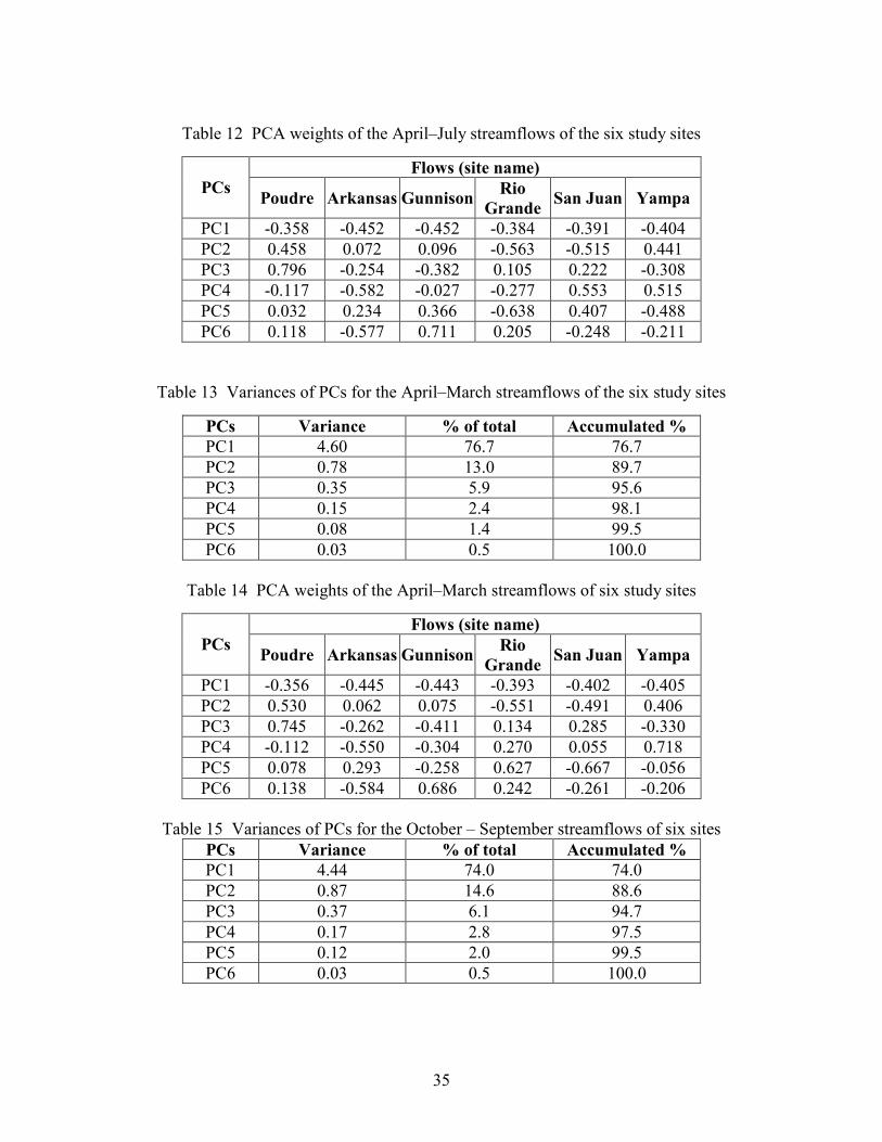
35

Table 12 PCA weights of the April–July streamflows of the six study sites

Flows (site name)

PCs Poudre Arkansas Gunnison

Rio

Grande San Juan Yampa

PC1 -0.358 -0.452 -0.452 -0.384 -0.391 -0.404

PC2 0.458 0.072 0.096 -0.563 -0.515 0.441

PC3 0.796 -0.254 -0.382 0.105 0.222 -0.308

PC4 -0.117 -0.582 -0.027 -0.277 0.553 0.515

PC5 0.032 0.234 0.366 -0.638 0.407 -0.488

PC6 0.118 -0.577 0.711 0.205 -0.248 -0.211

Table 13 Variances of PCs for the April–March streamflows of the six study sites

PCs Variance % of total Accumulated %

PC1 4.60 76.7 76.7

PC2 0.78 13.0 89.7

PC3 0.35 5.9 95.6

PC4 0.15 2.4 98.1

PC5 0.08 1.4 99.5

PC6 0.03 0.5 100.0

Table 14 PCA weights of the April–March streamflows of six study sites

Flows (site name)

PCs Poudre Arkansas Gunnison

Rio

Grande San Juan Yampa

PC1 -0.356 -0.445 -0.443 -0.393 -0.402 -0.405

PC2 0.530 0.062 0.075 -0.551 -0.491 0.406

PC3 0.745 -0.262 -0.411 0.134 0.285 -0.330

PC4 -0.112 -0.550 -0.304 0.270 0.055 0.718

PC5 0.078 0.293 -0.258 0.627 -0.667 -0.056

PC6 0.138 -0.584 0.686 0.242 -0.261 -0.206

Table 15 Variances of PCs for the October – September streamflows of six sites

PCs Variance % of total Accumulated %

PC1 4.44 74.0 74.0

PC2 0.87 14.6 88.6

PC3 0.37 6.1 94.7

PC4 0.17 2.8 97.5

PC5 0.12 2.0 99.5

PC6 0.03 0.5 100.0

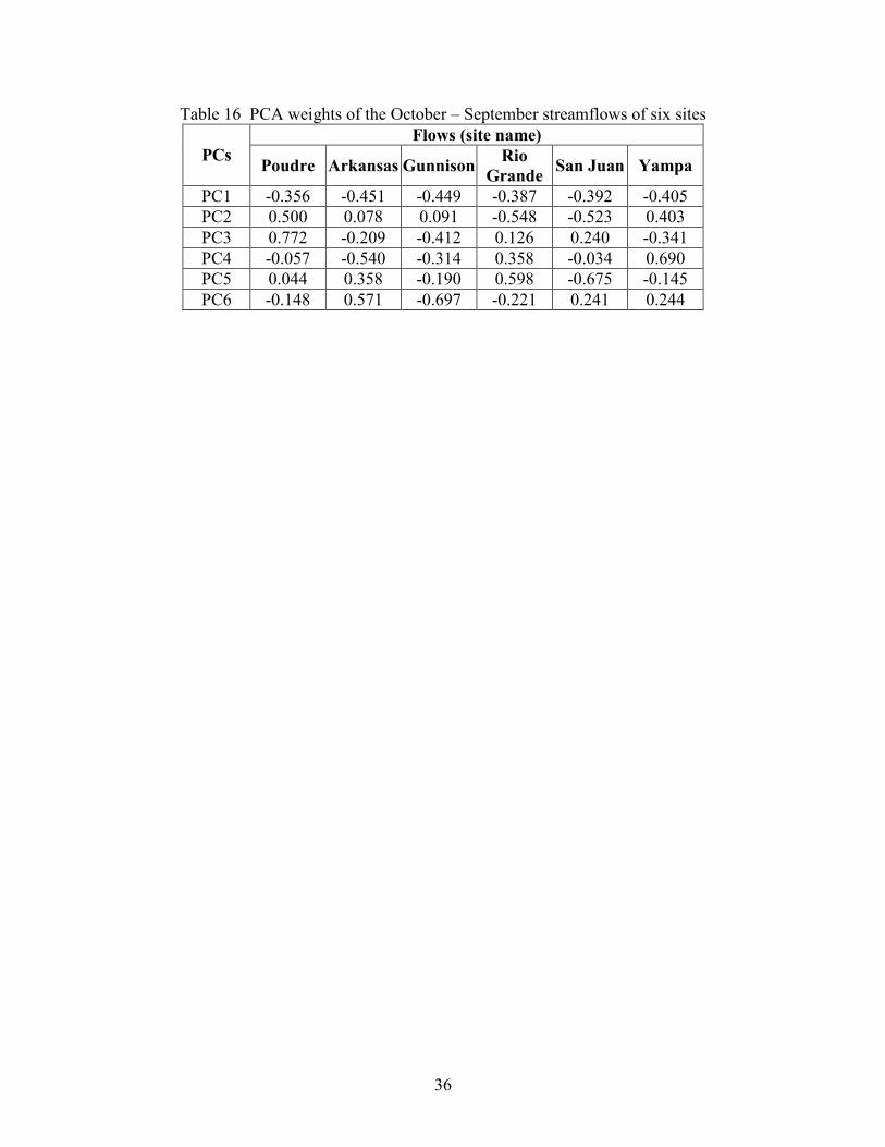
36

Table 16 PCA weights of the October – September streamflows of six sites

Flows (site name)

PCs Poudre Arkansas Gunnison

Rio

Grande San Juan Yampa

PC1 -0.356 -0.451 -0.449 -0.387 -0.392 -0.405

PC2 0.500 0.078 0.091 -0.548 -0.523 0.403

PC3 0.772 -0.209 -0.412 0.126 0.240 -0.341

PC4 -0.057 -0.540 -0.314 0.358 -0.034 0.690

PC5 0.044 0.358 -0.190 0.598 -0.675 -0.145

PC6 -0.148 0.571 -0.697 -0.221 0.241 0.244

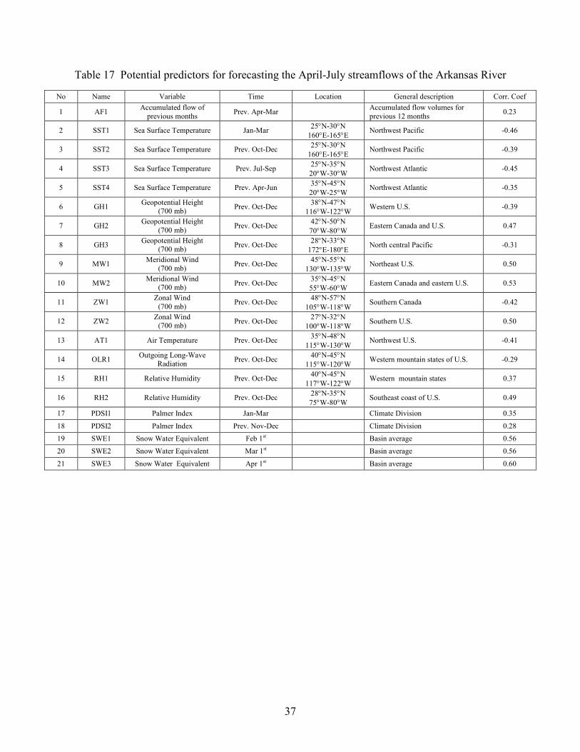
37

Table 17 Potential predictors for forecasting the April-July streamflows of the Arkansas River

No Name Variable Time Location General description Corr. Coef

1 AF1 Accumulated flow of

previous months Prev. Apr-Mar

Accumulated flow volumes for

previous 12 months 0.23

2 SST1 Sea Surface Temperature Jan-Mar 25°N-30°N

160°E-165°E Northwest Pacific -0.46

3 SST2 Sea Surface Temperature Prev. Oct-Dec 25°N-30°N

160°E-165°E Northwest Pacific -0.39

4 SST3 Sea Surface Temperature Prev. Jul-Sep 25°N-35°N

20°W-30°W Northwest Atlantic -0.45

5 SST4 Sea Surface Temperature Prev. Apr-Jun 35°N-45°N

20°W-25°W Northwest Atlantic -0.35

6 GH1 Geopotential Height

(700 mb) Prev. Oct-Dec

38°N-47°N

116°W-122°W Western U.S. -0.39

7 GH2 Geopotential Height

(700 mb) Prev. Oct-Dec

42°N-50°N

70°W-80°W Eastern Canada and U.S. 0.47

8 GH3 Geopotential Height

(700 mb) Prev. Oct-Dec

28°N-33°N

172°E-180°E North central Pacific -0.31

9 MW1 Meridional Wind

(700 mb) Prev. Oct-Dec

45°N-55°N

130°W-135°W Northeast U.S. 0.50

10 MW2 Meridional Wind

(700 mb) Prev. Oct-Dec

35°N-45°N

55°W-60°W Eastern Canada and eastern U.S. 0.53

11 ZW1 Zonal Wind

(700 mb) Prev. Oct-Dec

48°N-57°N

105°W-118°W Southern Canada -0.42

12 ZW2 Zonal Wind

(700 mb) Prev. Oct-Dec

27°N-32°N

100°W-118°W Southern U.S. 0.50

13 AT1 Air Temperature Prev. Oct-Dec 35°N-48°N

115°W-130°W Northwest U.S. -0.41

14 OLR1 Outgoing Long-Wave

Radiation Prev. Oct-Dec

40°N-45°N

115°W-120°W Western mountain states of U.S. -0.29

15 RH1 Relative Humidity Prev. Oct-Dec 40°N-45°N

117°W-122°W Western mountain states 0.37

16 RH2 Relative Humidity Prev. Oct-Dec 28°N-35°N

75°W-80°W Southeast coast of U.S. 0.49

17 PDSI1 Palmer Index Jan-Mar Climate Division 0.35

18 PDSI2 Palmer Index Prev. Nov-Dec Climate Division 0.28

19 SWE1 Snow Water Equivalent Feb 1st Basin average 0.56

20 SWE2 Snow Water Equivalent Mar 1st Basin average 0.56

21 SWE3 Snow Water Equivalent Apr 1st Basin average 0.60

38

Table 18 Potential predictors for forecasting the April-March streamflows of the Gunnison river

No Name Variable Time Location General description Corr. Coef

1 AF1 Lag-1 flow Prev. Apr-Mar 0.15

2 SST1 Sea Surface Temperature Jan-Mar 46°N-51°N

160°W-170°W Northeast Pacific 0.48

3 SST2 Sea Surface Temperature Jan-Mar 25°N-30°N

165°E-175°E Northwestl Pacific -0.39

4 SST3 Sea Surface Temperature Prev. Oct-Dec 43°N-48°N

170°W-175°W Northeast Pacific 0.41

5 SST4 Sea Surface Temperature Prev. Oct-Dec 26°N-31°N

165°E-170°E Northwest Pacific -0.41

6 SST5 Sea Surface Temperature Prev. Jul-Sep 27°N-32°N

25°W-30°W Northeast Atlantic -0.42

7 SSST1 Seesaw SST Jan-Mar SST1-SST2 0.49

8 SSST2 Seesaw SST Prev. Oct-Dec SST3-SST4 0.52

9 GH1 Geopotential Height

(700 mb) Jan-Mar

30°N-40°N

130°E-140°E Northwest Pacific -0.32

10 GH2 Geopotential Height

(700 mb) Prev. Oct-Dec

32°N-50°N

110°W-120°W Over U.S. -0.40

11 GH3 Geopotential Height

(700 mb) Prev. Oct-Dec

45°N-52°N

66°W-75°W Southeast Canada 0.44

12 GH4 Geopotential Height

(700 mb) Prev. Oct-Dec

27°N-32°N

175°E-180°E North central Pacific -0.35

13 GH5 Geopotential Height

(700 mb) Prev. Jul-Sep

30°N-35°N

160°E-165°E North central Pacific -0.36

14 GH6 Geopotential Height

(700 mb) Prev. Apr-Jun

50°N-60°N

80°W-85°W Northwest PAcific -0.29

15 MW1 Meridional Wind

(700 mb) Prev. Oct-Dec

42°N-47°N

85°W-95°W Northeast U.S. 0.49

16 MW2 Meridional Wind

(700 mb) Prev. Oct-Dec

45°N-50°N

125°W-130°W West coast of Canada -0.33

17 MW3 Meridional Wind

(700 mb) Prev. Oct-Dec

38°N-47°N

55°W-60°W Northwest Atlantic -0.38

18 ZW1 Zonal Wind

(700 mb) Jan-Mar

23°N-28°N

130°E-140°E Northwest Pacific 0.38

19 ZW2 Zonal Wind

(700 mb) Prev. Oct-Dec

28°N-33°N

105°W-115°W South U.S. 0.44

20 ZW3 Zonal Wind

(700 mb) Prev. Oct-Dec

50°N-55°N

110°W-115°W South Canada -0.39

21 AT1 Air Temperature Prev. Oct-Dec 47°N-52°N

110°W-120°W Northwest U.S. -0.49

22 AT2 Air Temperature Prev. Jul-Sep 26°N-31°N

115°W-120°W West coast of Mexico 0.32

23 AT3 Air Temperature Prev. Apr-Jun 47°N-52°N

70°W-85°W Southeast Canada -0.32

24 OLR1 Outgoing Long-Wave

Radiation Prev. Oct-Dec

35°N-44°N

110°W-120°W Southwest U.S. -0.44

25 OLR2 Outgoing Long-Wave

Radiation Prev. Apr-Jun

41°N-46°N

85°W-95°W Northeast U.S. -0.32

26 RH1 Relative Humidity Prev. Oct-Dec 40°N-45°N

11°W-120°W West U.S. 0.39

27 RH2 Relative Humidity Prev. Oct-Dec 30°N-35°N

75°W-80°W Southeast U.S. 0.51

28 RH3 Relative Humidity Prev. Oct-Dec 27°N-32°N

160°W-165°W Northeast Pacific 0.35

29 SWMR1 Southwest Monsoon

Rainfall Jan-Mar Arizona and New Mexico rainfall 0.33

30 SWE1 Snow Water Equivalent Feb 1st Basin average 0.71

31 SWE2 Snow Water Equivalent Mar 1st Basin average 0.73

32 SWE3 Snow Water Equivalent Apr 1st Basin average 0.82

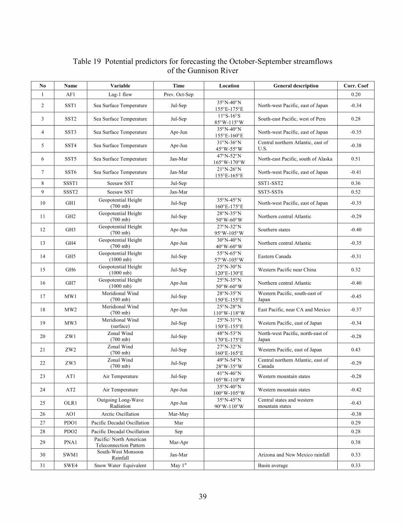
39

Table 19 Potential predictors for forecasting the October-September streamflows

of the Gunnison River

No Name Variable Time Location General description Corr. Coef

1 AF1 Lag-1 flow Prev. Oct-Sep 0.20

2 SST1 Sea Surface Temperature Jul-Sep 35°N-40°N

155°E-175°E North-west Pacific, east of Japan -0.34

3 SST2 Sea Surface Temperature Jul-Sep 11°S-16°S

85°W-115°W South-east Pacific, west of Peru 0.28

4 SST3 Sea Surface Temperature Apr-Jun 35°N-40°N

155°E-160°E North-west Pacific, east of Japan -0.35

5 SST4 Sea Surface Temperature Apr-Jun 31°N-36°N

45°W-55°W

Central northern Atlantic, east of

U.S. -0.38

6 SST5 Sea Surface Temperature Jan-Mar 47°N-52°N

165°W-170°W North-east Pacific, south of Alaska 0.51

7 SST6 Sea Surface Temperature Jan-Mar 21°N-26°N

155°E-165°E North-west Pacific, east of Japan -0.41

8 SSST1 Seesaw SST Jul-Sep SST1-SST2 0.36

9 SSST2 Seesaw SST Jan-Mar SST5-SST6 0.52

10 GH1 Geopotential Height

(700 mb) Jul-Sep

35°N-45°N

160°E-175°E North-west Pacific, east of Japan -0.35

11 GH2 Geopotential Height

(700 mb) Jul-Sep

28°N-35°N

50°W-60°W Northern central Atlantic -0.29

12 GH3 Geopotential Height

(700 mb) Apr-Jun

27°N-32°N

95°W-105°W Southern states -0.40

13 GH4 Geopotential Height

(700 mb) Apr-Jun

30°N-40°N

40°W-60°W Northern central Atlantic -0.35

14 GH5 Geopotential Height

(1000 mb) Jul-Sep

55°N-65°N

57°W-105°W Eastern Canada -0.31

15 GH6 Geopotential Height

(1000 mb) Jul-Sep

25°N-30°N

120°E-130°E Western Pacific near China 0.32

16 GH7 Geopotential Height

(1000 mb) Apr-Jun

25°N-35°N

50°W-60°W Northern central Atlantic -0.40

17 MW1 Meridional Wind

(700 mb) Jul-Sep

28°N-35°N

150°E-155°E

Western Pacific, south-east of

Japan -0.45

18 MW2 Meridional Wind

(700 mb) Apr-Jun

25°N-28°N

110°W-118°W East Pacific, near CA and Mexico -0.37

19 MW3 Meridional Wind

(surface) Jul-Sep

25°N-31°N

150°E-155°E Western Pacific, east of Japan -0.34

20 ZW1 Zonal Wind

(700 mb) Jul-Sep

48°N-53°N

170°E-175°E

North-west Pacific, north-east of

Japan -0.28

21 ZW2 Zonal Wind

(700 mb) Jul-Sep

27°N-32°N

160°E-165°E Western Pacific, east of Japan 0.43

22 ZW3 Zonal Wind

(700 mb) Jul-Sep

49°N-54°N

28°W-35°W

Central northern Atlantic, east of

Canada -0.29

23 AT1 Air Temperature Jul-Sep 41°N-46°N

105°W-110°W Western mountain states -0.28

24 AT2 Air Temperature Apr-Jun 35°N-40°N

100°W-105°W Western mountain states -0.42

25 OLR1 Outgoing Long-Wave

Radiation Apr-Jun

35°N-45°N

90°W-110°W

Central states and western

mountain states -0.43

26 AO1 Arctic Oscillation Mar-May -0.38

27 PDO1 Pacific Decadal Oscillation Mar 0.29

28 PDO2 Pacific Decadal Oscillation Sep 0.28

29 PNA1 Pacific/ North American

Teleconnection Pattern Mar-Apr 0.38

30 SWM1 South-West Monsoon

Rainfall Jan-Mar Arizona and New Mexico rainfall 0.33

31 SWE4 Snow Water Equivalent May 1st Basin average 0.33

40

Table 20 Selected predictors for forecasting the April–July streamflows for the six study sites

No. River Name Variable Time Corr. Coef.

1 SST8 Sea Surface

Temperature Prev. Apr-Jun -0.29

2 ZW3 Zonal Wind

(700 mb) Jan-Mar 0.41

3

Poudre

SWE3 Snow Water

Equivalent Apr 1st 0.65

4 SST4 Sea Surface

Temperature Prev. Jul-Sep -0.45

5 MW2 Meridional Wind

(700 mb) Prev. Oct-Dec -0.53

6 RH2 Relative Humidity Prev. Oct-Dec 0.49

7

Arkansas

SWE3 Snow Water

Equivalent Apr 1st 0.60

8 SST2 Sea Surface

Temperature Jan-Mar -0.45

9 SST7 Sea Surface

Temperature Prev. Apr-Jun 0.40

10 SST9 Sea Surface

Temperature Prev. Apr-Jun -0.31

11 GH5 Geopotential Height

(700 mb) Prev. Oct-Dec -0.35

12 RH4 Relative Humidity Prev. Oct-Dec 0.36

13 ZW2 Zonal Wind

(700 mb) Jan-Mar 0.34

14 PDSI1 Palmer Index Jan-Mar 0.70

15

Gunnison

SWE3 Snow Water

Equivalent Apr 1st 0.85

16 SSST1 Seesaw SST Jan-Mar 0.54

17 GH6 Geopotential Height

(700 mb) Prev. Oct-Dec -0.51

18 ZW4 Zonal Wind

(700 mb) Prev. Oct-Dec -0.47

19 RH2 Relative Humidity Prev. Oct-Dec 0.60

20

Rio Grande

SWE3 Snow Water

Equivalent Apr 1st 0.65

21 GH3 Geopotential Height

(700 mb) Prev. Oct-Dec 0.40

22 GH5 Geopotential Height

(700 mb) Prev. Jul-Sep -0.42

23 OLR1 Outgoing Long-Wave

Radiation Jan-Mar -0.58

24 OLR2 Outgoing Long-Wave

Radiation Prev. Oct-Dec -0.48

25

San Juan

SWE3 Snow Water

Equivalent Mar 1st 0.85

26 GH1 Geopotential Height

(700 mb) Jan-Mar -0.43

27 MW3 Meridional Wind

(700 mb) Prev. Oct-Dec -0.41

28 OLR3 Outgoing Long-Wave

Radiation Prev. Oct-Dec -0.49

29 PDSI1 Palmer Index Jan-Mar 0.66

30 PDSI2 Palmer Index Prev. Oct-Dec 0.40

31

Yampa

SWE2 Snow Water

Equivalent Mar 1st 0.57

41

Table 21 Forecast equations based on MLR for forecasting the April-July streamflows

for the six study sites

Site Equations

Poudre River z = − 0.24 × SST8(A-J) + 0.412 × ZW3(J-M) + 0.616 × SWE3(Apr 1st)

Arkansas River z = − 0.294 × SST4(J-S) − 0.140 × MW2(O-D) + 0.423× RH(O-D) + 0.392 × SWE3(Apr 1st)

Gunnison River z = 0.192 × SST2(J-M) + 0.124 × SST7(A-J) − 0.194 × SST9(A-J) − 0.231 × GH5(O-D) +

0.209 × ZW2(J-M) + 0.203 × RH4(O-D) + 0.288 × PDSI1(J-M) + 0.518 × SWE3(Apr 1st)

Rio Grande z = 0.249 × SSST1(J-M) − 0.213 × GH6(O-D) − 0.176 × ZW4(O-D) + 0.360 × RH2(O-D) +

0.425 × SWE3(Apr 1st)

San Juan River z = 0.187 × GH3(O-D) − 0.172 × GH5(J-S) − 0.170 × OLR1(J-M) − 0.130 × OLR2(O-D) +

0.623 × SWE3(Apr 1st)

Yampa River z = − 0.307 × GH1(J-M) − 0.174 × MW3(O-D) − 0.235 × OLR2(J-M) + 0.829 × PDSI1(J-

M) – 0.583 × PDSI2(O-D) + 0.273× SWE2(Mar 1st)

Note: The parenthesis in the equations indicate the time period. For example, SST8(A-J)

indicates the SST for the time period April-June of the previous year (refer to Table 13).

Table 22a Forecast model performance for single site based on MLR

Method Item Poudre Arkansas Gunnison Rio Grande San Juan Yampa

R2 0.64 0.64 0.89 0.83 0.85 0.81

Fitting adj. R

2 0.62 0.60 0.87 0.81 0.83 0.79

R2 0.52 0.52 0.83 0.77 0.79 0.72

Drop one adj. R

2 0.49 0.48 0.80 0.75 0.77 0.68

Table 22b Forecast skill scores for single site MLR models Method Item Poudre Arkansas Gunnison Rio Grande San Juan Yampa

Accuracy 0.53 0.53 0.72 0.68 0.64 0.72 Fitting

HSS 0.37 0.37 0.62 0.57 0.52 0.62

Accuracy 0.49 0.53 0.68 0.68 0.60 0.66 Drop one

HSS 0.32 0.37 0.57 0.57 0.47 0.55

Table 23a Cross-correlation coefficient for single site MLR models (fitting) Sites Poudre Arkansas Gunnison Rio Grande San Juan Yampa

Poudre 1 0.58 0.58 0.42 0.35 0.63

Arkansas 0.58 1 0.80 0.67 0.61 0.73

Gunnison 0.58 0.80 1 0.65 0.72 0.88

Rio Grande 0.42 0.67 0.65 1 0.84 0.53

San Juan 0.35 0.61 0.72 0.84 1 0.60

Yampa 0.63 0.73 0.88 0.53 0.60 1

42

Table 23b Cross-correlation coefficient for single site MLR models (drop one) Sites Poudre Arkansas Gunnison Rio Grande San Juan Yampa

Poudre 1 0.54 0.58 0.41 0.32 0.61

Arkansas 0.54 1 0.74 0.64 0.57 0.67

Gunnison 0.58 0.74 1 0.63 0.69 0.85

Rio Grande 0.41 0.64 0.63 1 0.82 0.53

San Juan 0.32 0.57 0.69 0.82 1 0.59

Yampa 0.61 0.67 0.85 0.53 0.59 1

Table 24 Variances of PCs for April–July streamflows of Poudre River

PCs Variance % Accum

% PCs Variance %

Accum

%

1 10.05 27.9 27.9 19 0.31 0.9 95.1

2 4.95 13.7 41.7 20 0.29 0.8 95.9

3 2.66 7.4 49.1 21 0.27 0.7 96.6

4 2.35 6.5 55.6 22 0.24 0.7 97.3

5 2.08 5.8 61.4 23 0.18 0.5 97.8

6 1.70 4.7 66.1 24 0.14 0.4 98.2

7 1.57 4.4 70.4 25 0.13 0.4 98.6

8 1.28 3.6 74.0 26 0.11 0.3 98.9

9 1.17 3.3 77.3 27 0.10 0.3 99.1

10 1.12 3.1 80.4 28 0.08 0.2 99.4

11 0.97 2.7 83.0 29 0.07 0.2 99.5

12 0.76 2.1 85.2 30 0.05 0.1 99.7

13 0.73 2.0 87.2 31 0.04 0.1 99.8

14 0.66 1.8 89.0 32 0.03 0.1 99.9

15 0.55 1.5 90.5 33 0.02 0.1 99.9

16 0.51 1.4 92.0 34 0.01 0.0 100.0

17 0.44 1.2 93.2 35 0.01 0.0 100.0

18 0.38 1.1 94.2 36 0.00 0.0 100.0

Table 25 Model parameters of PCA model for each site

Table 26a Model performance for single site PCA models

Method Item Poudre Arkansas Gunnison Rio Grande San Juan Yampa

R2 0.67 0.70 0.87 0.86 0.85 0.88

Fitting adj. R

2 0.63 0.66 0.85 0.84 0.83 0.87

R2 0.54 0.58 0.76 0.73 0.77 0.79

Drop one adj. R

2 0.49 0.54 0.73 0.70 0.74 0.77

Poudre Arkansas Gunnison Rio Grande San Juan Yampa

PCs beta PCs beta PCs beta PCs beta PCs beta PCs beta

PC1 -0.645 PC1 -0.731 PC1 -0.788 PC1 -0.809 PC1 -0.837 PC1 0.815

PC2 -0.315 PC3 0.189 PC2 -0.230 PC2 0.263 PC2 0.136 PC2 0.160

PC4 -0.173 PC4 -0.371 PC3 0.174 PC3 0.254 PC3 -0.143 PC3 0.190

PC10 0.228 PC10 -0.169 PC4 0.245 PC6 -0.160 PC7 -0.115 PC12 -0.163

PC12 -0.197 PC12 0.177 PC6 0.146 PC9 -0.152 PC8 -0.223 PC17 0.256

PC12 0.162 PC11 0.115

43

Table 26b Forecast skill scores for single site PCA models

Method Item Poudre Arkansas Gunnison Rio Grande San Juan Yampa

Accuracy 0.55 0.57 0.60 0.66 0.74 0.70 Fitting

HSS 0.39 0.42 0.47 0.56 0.65 0.60

Accuracy 0.49 0.53 0.57 0.58 0.68 0.62 Drop one

HSS 0.32 0.37 0.42 0.46 0.57 0.50

Table 27a Cross-correlation coefficient for single site PCA models (fitting)

Sites Poudre Arkansas Gunnison Rio Grande San Juan Yampa

Poudre 1 0.66 0.65 0.45 0.48 0.72

Arkansas 0.66 1 0.83 0.65 0.65 0.76

Gunnison 0.65 0.83 1 0.63 0.70 0.88

Rio Grande 0.45 0.65 0.63 1 0.86 0.56

San Juan 0.48 0.65 0.70 0.86 1 0.61

Yampa 0.72 0.76 0.88 0.56 0.61 1

Table 27b Cross-correlation coefficient for single site PCA models (drop one)

Sites Poudre Arkansas Gunnison Rio Grande San Juan Yampa

Poudre 1 0.67 0.66 0.45 0.48 0.72

Arkansas 0.67 1 0.78 0.61 0.64 0.72

Gunnison 0.66 0.78 1 0.60 0.67 0.86

Rio Grande 0.45 0.61 0.60 1 0.82 0.56

San Juan 0.48 0.64 0.67 0.82 1 0.61

Yampa 0.72 0.72 0.86 0.56 0.61 1

Table 28 Parameters of the forecast model that only use climatic variables

for the April–July streamflows of Gunnison River

Table 29 Model performance for the model that only use climatic variables for the

April–July streamflows of Gunnison River

Values of R2 Values of skill scores

Method Item Values Item Values

R2 0.63 Accuracy 0.47

Fitting adj. R

2 0.61 HSS 0.30

R2 0.53 Accuracy 0.47

Drop one adj. R

2 0.50 HSS 0.30

PCs beta

PC1 0.717

PC2 0.177

PC5 -0.299

44

Table 30 Variances of PCs obtained from all potential predictors for 6 sites

PCs Variance % Accumulated

% PCs Variance %

Accumulated

% PCs Variance %

Accumulated

%

1 51.7 25.1 25.1 26 1.4 0.7 92.5 52 0.2 0.1 100.0

2 23.4 11.4 36.5 27 1.2 0.6 93.1 53 ~ 207 0.0 0.0 100.0

3 15.0 7.3 43.7 28 1.2 0.6 93.7

4 12.1 5.9 49.6 29 1.1 0.5 94.2

5 11.4 5.6 55.2 30 1.0 0.5 94.7

6 9.9 4.8 60.0 31 1.0 0.5 95.2

7 7.8 3.8 63.8 32 1.0 0.5 95.6

8 6.5 3.1 66.9 33 0.9 0.4 96.1

9 5.9 2.9 69.8 34 0.8 0.4 96.5

10 5.1 2.5 72.3 35 0.7 0.4 96.8

11 4.7 2.3 74.5 36 0.7 0.3 97.1

12 4.0 1.9 76.5 37 0.7 0.3 97.5

13 3.8 1.8 78.3 38 0.6 0.3 97.7

14 3.4 1.7 80.0 39 0.6 0.3 98.0

15 3.2 1.6 81.5 40 0.5 0.2 98.3

16 2.9 1.4 83.0 41 0.5 0.2 98.5

17 2.6 1.3 84.2 42 0.4 0.2 98.7

18 2.4 1.2 85.4 43 0.4 0.2 98.9

19 2.3 1.1 86.5 44 0.4 0.2 99.1

20 2.1 1.0 87.5 45 0.3 0.2 99.2

21 2.0 1.0 88.5 46 0.3 0.1 99.4

22 1.9 0.9 89.4 47 0.3 0.1 99.5

23 1.8 0.9 90.3 48 0.3 0.1 99.7

24 1.6 0.8 91.0 49 0.2 0.1 99.8

25 1.6 0.8 91.8 50 0.2 0.1 99.8

Table 31a Model performance for multisite CCA models

Method Item Poudre Arkansas Gunnison Rio Grande San Juan Yampa

R2 0.58 0.78 0.78 0.76 0.75 0.82

Fitting adj. R

2 0.52 0.74 0.74 0.71 0.68 0.80

R2 0.41 0.63 0.64 0.69 0.62 0.71

Drop one adj. R

2 0.33 0.57 0.56 0.63 0.52 0.67

Table 31b Forecast skill scores for multisite CCA models

Method Item Poudre Arkansas Gunnison Rio Grande San Juan Yampa

Accuracy 0.47 0.57 0.53 0.60 0.60 0.66 Fitting

HSS 0.29 0.42 0.37 0.47 0.47 0.55

Accuracy 0.43 0.57 0.49 0.57 0.55 0.57 Drop one

HSS 0.24 0.42 0.32 0.42 0.40 0.42

Table 32a Cross-correlation coefficient for multisite CCA models (fitting)

Sites Poudre Arkansas Gunnison Rio Grande San Juan Yampa

Poudre 1 0.78 0.78 0.48 0.53 0.85

Arkansas 0.78 1 0.96 0.68 0.73 0.91

45

Gunnison 0.78 0.96 1 0.64 0.76 0.93

Rio Grande 0.48 0.68 0.64 1 0.92 0.47

San Juan 0.53 0.73 0.76 0.92 1 0.55

Yampa 0.85 0.91 0.93 0.47 0.55 1

Table 32b Cross-correlation coefficient for multisite CCA models (drop one)

Sites Poudre Arkansas Gunnison Rio Grande San Juan Yampa

Poudre 1 0.67 0.66 0.39 0.50 0.77

Arkansas 0.67 1 0.78 0.50 0.67 0.73

Gunnison 0.66 0.78 1 0.39 0.65 0.81

Rio Grande 0.39 0.50 0.39 1 0.85 0.40

San Juan 0.50 0.67 0.65 0.85 1 0.58

Yampa 0.77 0.73 0.81 0.40 0.58 1

Table 33a Model performance for the aggregation – disaggregation models

Method Item Poudre Arkansas Gunnison Rio Grande San Juan Yampa

R2 0.38 0.71 0.70 0.62 0.66 0.50

Fitting adj. R

2 0.30 0.66 0.64 0.55 0.57 0.43

R2 0.30 0.63 0.63 0.58 0.62 0.44

Drop one adj. R

2 0.19 0.57 0.57 0.51 0.51 0.35

Table 33b Forecast skill scores for the aggregation – disaggregation models

Method Item Poudre Arkansas Gunnison Rio Grande San Juan Yampa

Accuracy 0.34 0.64 0.51 0.55 0.34 0.47 Fitting

HSS 0.12 0.52 0.35 0.40 0.13 0.30

Accuracy 0.32 0.57 0.47 0.51 0.38 0.43 Drop one

HSS 0.10 0.42 0.30 0.35 0.18 0.24

Table 34a Cross-correlation coefficient for the aggregation – disaggregation models (fitting)

Sites Poudre Arkansas Gunnison Rio Grande San Juan Yampa

Poudre 1 0.70 0.65 0.46 0.54 0.51

Arkansas 0.70 1 0.92 0.71 0.72 0.70

Gunnison 0.65 0.92 1 0.62 0.67 0.74

Rio Grande 0.46 0.71 0.62 1 0.83 0.26

San Juan 0.54 0.72 0.67 0.83 1 0.33

Yampa 0.51 0.70 0.74 1.26 0.33 1

Table 34b Cross-correlation coefficient for the aggregation – disaggregation models (drop one)

Sites Poudre Arkansas Gunnison Rio Grande San Juan Yampa

Poudre 1 0.68 0.67 0.11 0.30 0.66

Arkansas 0.68 1 0.92 0.30 0.37 0.77

Gunnison 0.67 0.92 1 0.34 0.44 0.82

Rio Grande 0.11 0.30 0.34 1 0.82 0.18

San Juan 0.30 0.37 0.44 0.82 1 0.26

Yampa 0.66 0.77 0.82 0.18 0.26 1

46

Table 35 Model parameters for the April – March streamflow forecast of Gunnison River

Table 36 Model performance for the April – March streamflow forecast of Gunnison River

Values of R2 Values of skill scores

Method Item Values Item Values

R2 0.75 Accuracy 0.62

Fitting adj. R

2 0.73 HSS 0.50

R2 0.67 Accuracy 0.57

Drop one adj. R

2 0.64 HSS 0.42

Table 37 Model parameters for October – September streamflow forecast of Gunnison River

Table 38 Model performance for October – September streamflow forecast of Gunnison River

Values of R2 Values of skill scores

Method Item Values Item Values

R2 0.65 Accuracy 0.55

Fitting adj. R

2 0.62 HSS 0.40

R2 0.54 Accuracy 0.47

Drop one adj. R

2 0.50 HSS 0.30

PCs beta

PC1 -0.785

PC6 0.275

PC7 -0.175

PC11 0.165

PCs beta

PC1 -0.670

PC5 -0.271

PC10 -0.298

PC11 0.188

47

Table 41 RMSE of the CCA model using random drop-10% method

RMSE (AF) Method

Poudre Arkansas Gunnison Rio Grande San Juan Yampa

For fitting

part 55587 61714 137037 98003 196874 150513

For drop10%

part 71566 74480 173282 114357 229386 196312

Figure 1. Map of flow sites

48

0

20

40

60

80

100

PC1 PC2 PC3 PC4 PC5 PC6

PCs

% of total variances

Figure 2 Plot of the variances of PCs for the April–July streamflows of the 6 sites

-1.0

-0.5

0.0

0.5

1.0

Poudre Arkansas Gunnison Rio Grande San Juan Yampa

Flows

Weights

for PC1 for PC2

for PC3 for PC4

for PC5 for PC6

Figure 3 Plot of the weights for the April-July streamflows of the 6 sites

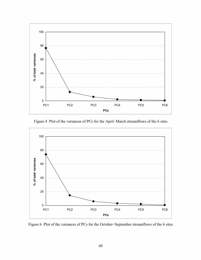
49

0

20

40

60

80

100

PC1 PC2 PC3 PC4 PC5 PC6

PCs

% of total variances

Figure 4 Plot of the variances of PCs for the April–March streamflows of the 6 sites

0

20

40

60

80

100

PC1 PC2 PC3 PC4 PC5 PC6

PCs

% of total variances

Figure 6 Plot of the variances of PCs for the October–September streamflows of the 6 sites

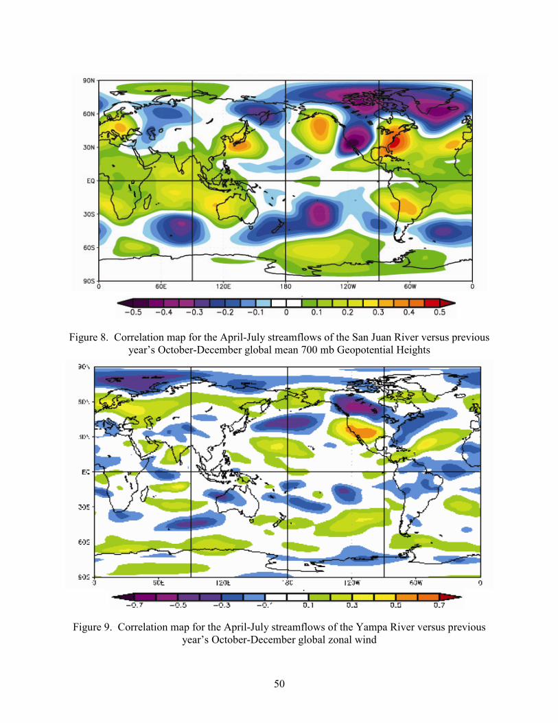
50

Figure 8. Correlation map for the April-July streamflows of the San Juan River versus previous

year’s October-December global mean 700 mb Geopotential Heights

Figure 9. Correlation map for the April-July streamflows of the Yampa River versus previous

year’s October-December global zonal wind

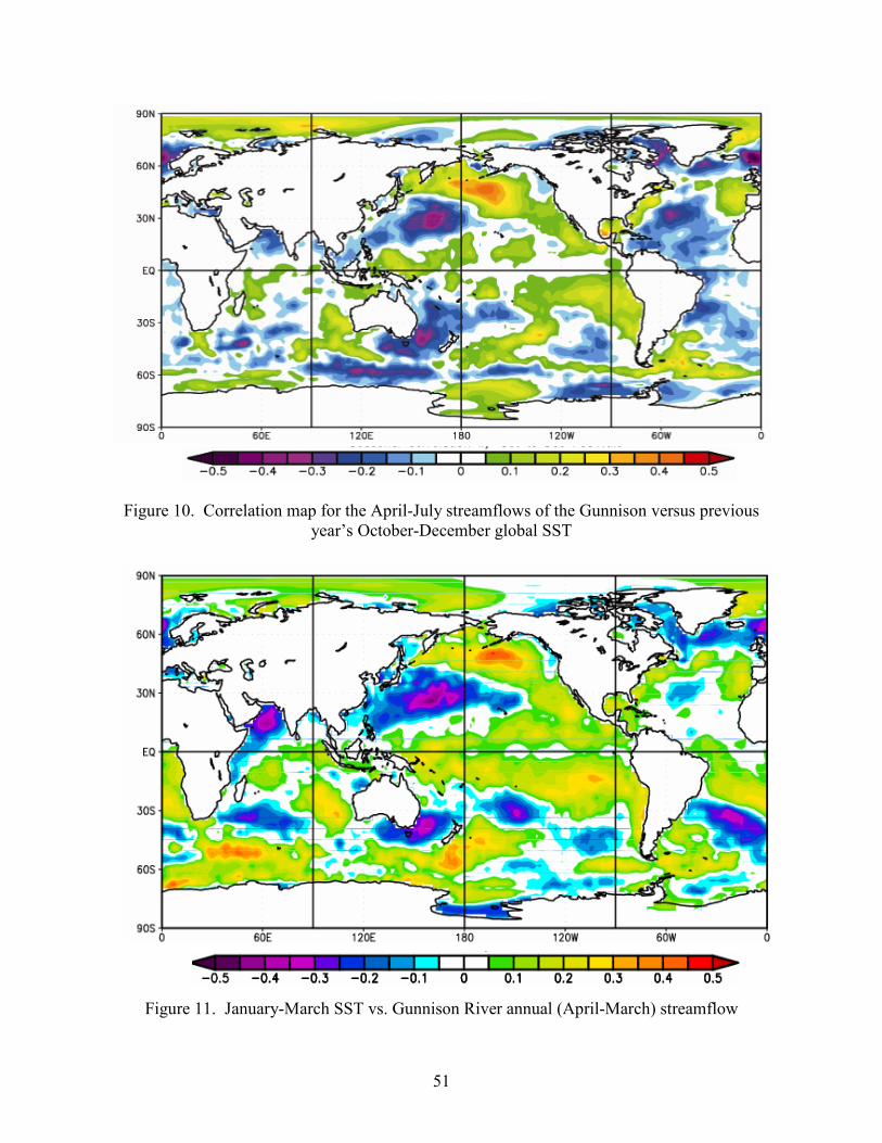
51

Figure 10. Correlation map for the April-July streamflows of the Gunnison versus previous

year’s October-December global SST

Figure 11. January-March SST vs. Gunnison River annual (April-March) streamflow

52

Figure 12. July-September SST vs. Gunnison River annual (October-September) streamflow

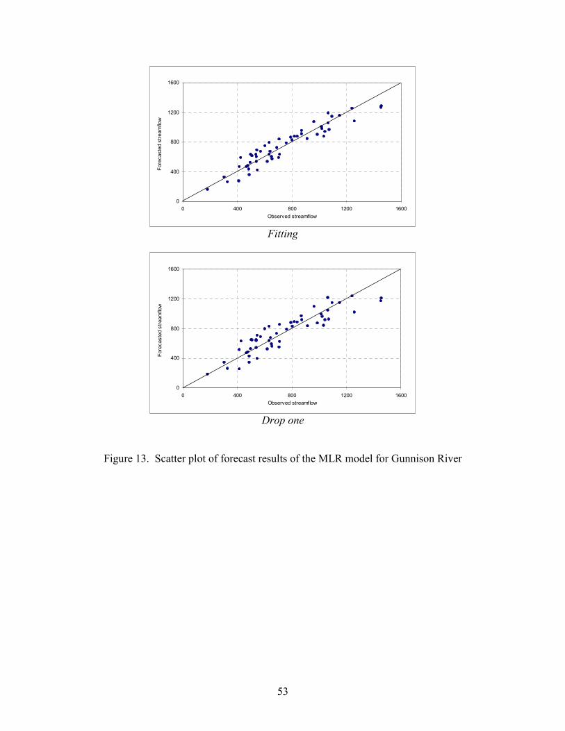
53

0

400

800

1200

1600

0 400 800 1200 1600

Observed streamflow

Fore

caste

d s

tream

flow

Fitting

0

400

800

1200

1600

0 400 800 1200 1600

Observed streamflow

Fore

caste

d s

tream

flow

Drop one

Figure 13. Scatter plot of forecast results of the MLR model for Gunnison River

54

0

400

800

1200

1600

1945 1950 1955 1960 1965 1970 1975 1980 1985 1990 1995 2000 2005

Years

Flo

w, T

AF

Observed

Forecast

Fitting

0

400

800

1200

1600

1945 1950 1955 1960 1965 1970 1975 1980 1985 1990 1995 2000 2005

Years

Flo

w, T

AF

Observed

Forecast

Drop one

Figure 14. Time series plots of the forecast results of MLR model for Gunnison River

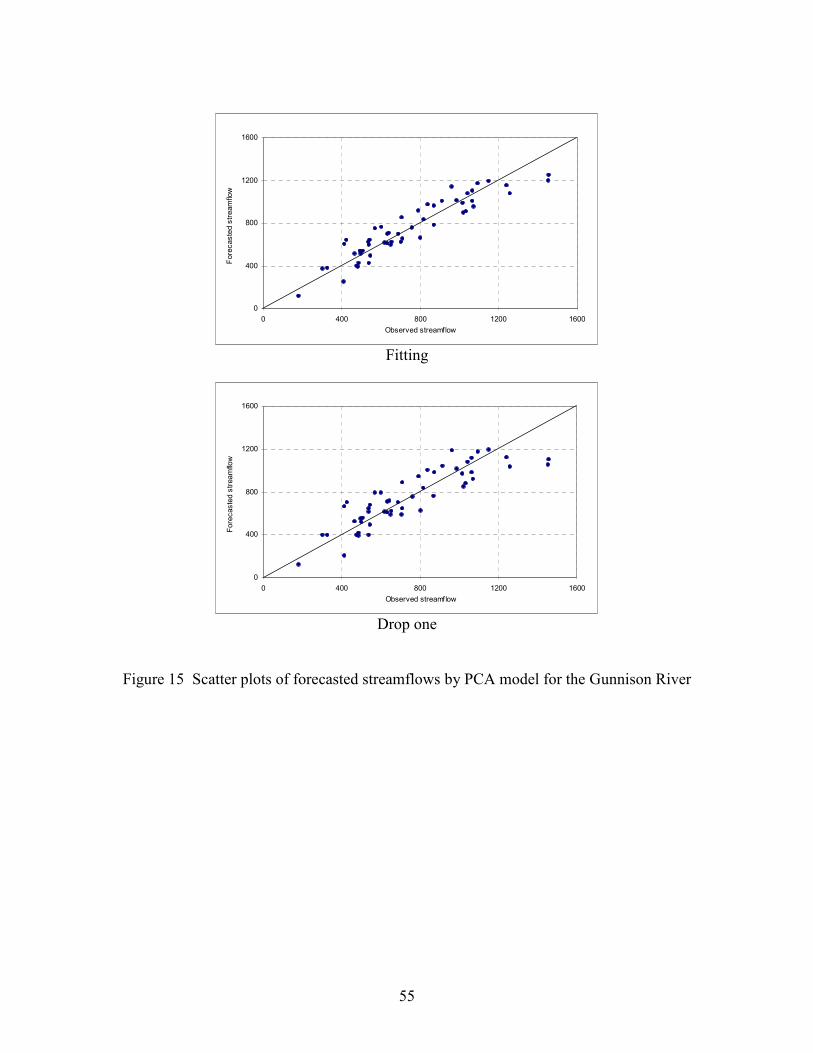
55

0

400

800

1200

1600

0 400 800 1200 1600

Observed streamflow

Fore

caste

d s

tream

flow

Fitting

0

400

800

1200

1600

0 400 800 1200 1600

Observed streamflow

Fore

caste

d s

tream

flow

Drop one

Figure 15 Scatter plots of forecasted streamflows by PCA model for the Gunnison River

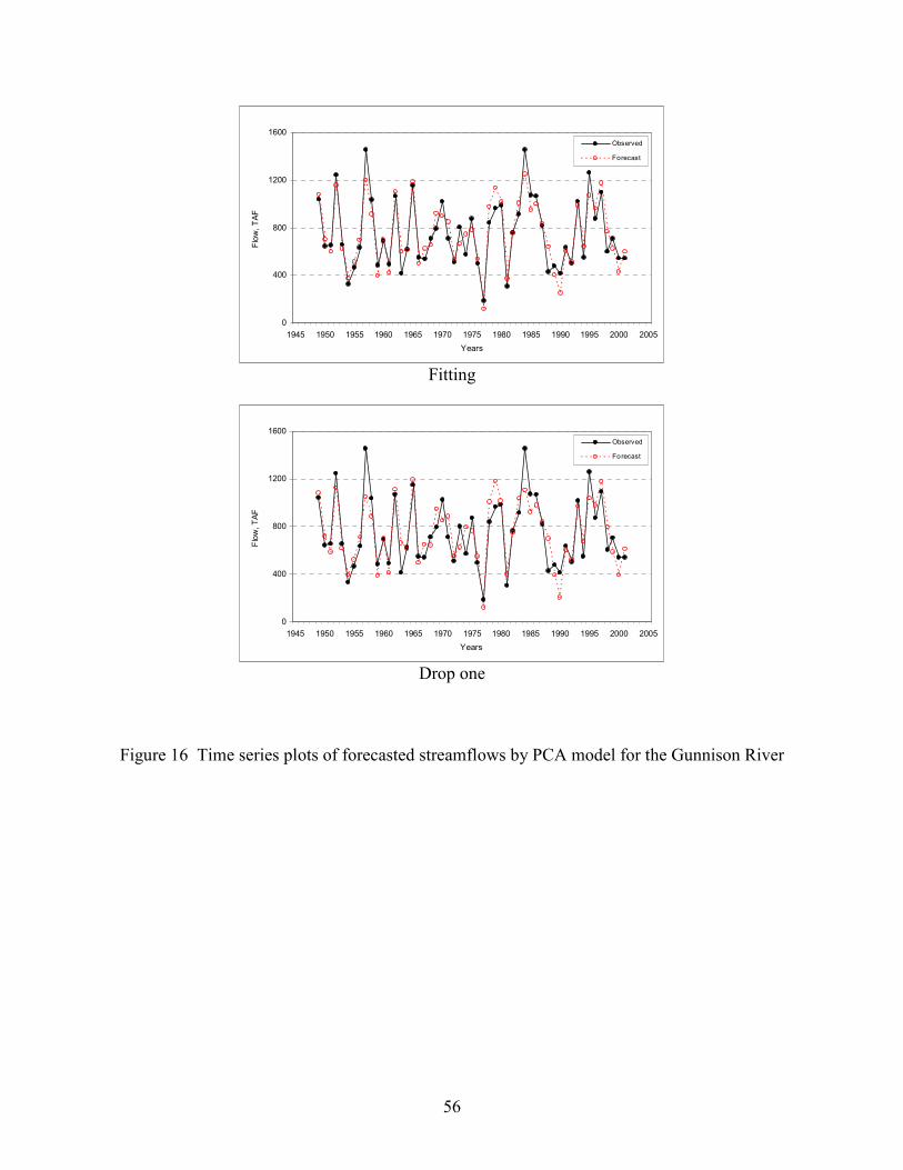
56

0

400

800

1200

1600

1945 1950 1955 1960 1965 1970 1975 1980 1985 1990 1995 2000 2005

Years

Flo

w, T

AF

Observed

Forecast

Fitting

0

400

800

1200

1600

1945 1950 1955 1960 1965 1970 1975 1980 1985 1990 1995 2000 2005

Years

Flo

w, T

AF

Observed

Forecast

Drop one

Figure 16 Time series plots of forecasted streamflows by PCA model for the Gunnison River

57

0.0

0.2

0.4

0.6

0.8

1.0

Poudre Arkansas Gunnison Rio Grande San Juan Yampa

Model performance for fitting

R-square

PCA model MLR model

Fitting

0.0

0.2

0.4

0.6

0.8

1.0

Poudre Arkansas Gunnison Rio Grande San Juan Yampa

Model performance for drop one

R-square

PCA model MLR model

Drop one

Figure 17a Comparison of R2 for the models in sections 6.3.1. and 6.3.2.

58

0.0

0.2

0.4

0.6

0.8

1.0

Poudre Arkansas Gunnison Rio Grande San Juan Yampa

Forecast skills for fitting

Accuracy

PCA model MLR model

Fitting

0.0

0.2

0.4

0.6

0.8

1.0

Poudre Arkansas Gunnison Rio Grande San Juan Yampa

Forecast skills for drop one

Accuracy

PCA model MLR model

Drop one

Figure 17b Comparison of forecast skills for the models in sections 6.3.1 and 6.3.2

59

0.0

0.2

0.4

0.6

0.8

1.0

Fitting Drop one Drop 10%

R-square

All variables Only climatic variables

R

2

0.0

0.2

0.4

0.6

0.8

1.0

Fitting Drop one Drop 10%

Accuray

All variables Only climatic variables

Accuracy

0.0

0.2

0.4

0.6

0.8

1.0

Fitting Drop one Drop 10%

HSS

All variables Only climatic variables

HSS

Figure 18. Comparison of R2 for the models in sections 6.3.2 and 6.3.3

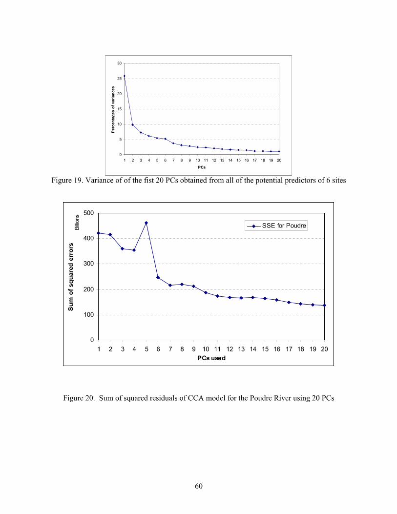
60

0

5

10

15

20

25

30

1 2 3 4 5 6 7 8 9 10 11 12 13 14 15 16 17 18 19 20

PCs

Percentages of variances

Figure 19. Variance of of the fist 20 PCs obtained from all of the potential predictors of 6 sites

0

100

200

300

400

500

1 2 3 4 5 6 7 8 9 10 11 12 13 14 15 16 17 18 19 20

Billio

ns

PCs used

Sum of squared errors

SSE for Poudre

Figure 20. Sum of squared residuals of CCA model for the Poudre River using 20 PCs

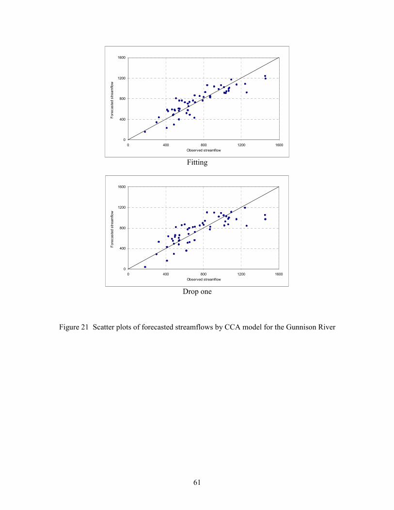
61

0

400

800

1200

1600

0 400 800 1200 1600

Observed streamflow

Fore

caste

d s

tream

flow

Fitting

0

400

800

1200

1600

0 400 800 1200 1600

Observed streamflow

Fore

cas

ted s

tre

am

flow

Drop one

Figure 21 Scatter plots of forecasted streamflows by CCA model for the Gunnison River

62

0

400

800

1200

1600

1945 1950 1955 1960 1965 1970 1975 1980 1985 1990 1995 2000 2005

Years

Flo

w,

TA

F

Observed

Forecast

Fitting

0

400

800

1200

1600

1945 1950 1955 1960 1965 1970 1975 1980 1985 1990 1995 2000 2005

Years

Flo

w, T

AF

Observed

Forecast

Drop one

Figure 22 Time series plots of forecasted streamflows by CCA model for the Gunnison River

63

0.0

0.2

0.4

0.6

0.8

1.0

Poudre Arkansas Gunnison Rio Grande San Juan Yampa

Model performance for fitting

R-square

PCA model CCA model

Fitting

0.0

0.2

0.4

0.6

0.8

1.0

Poudre Arkansas Gunnison Rio Grande San Juan Yampa

Model performance for drop one

R-square

PCA model CCA model

Drop one

Figure 23 Comparison of R2 for the forecast models based on PCA and CCA for Gunnison River

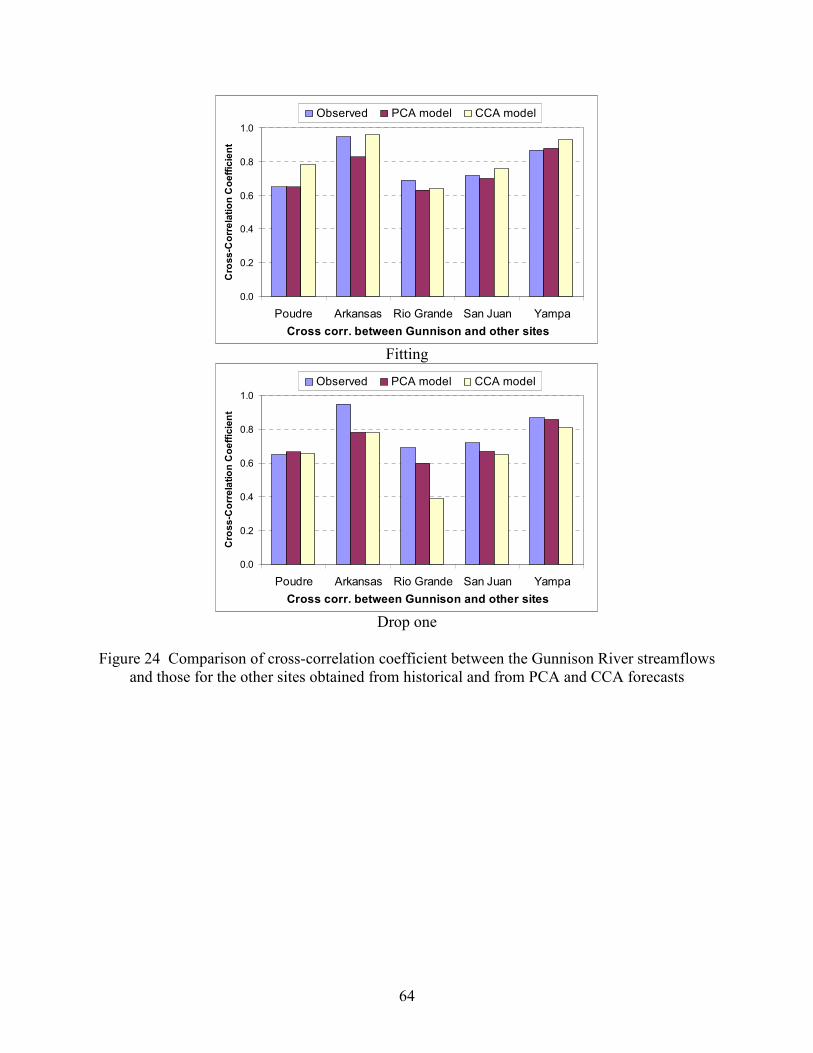
64

0.0

0.2

0.4

0.6

0.8

1.0

Poudre Arkansas Rio Grande San Juan Yampa

Cross corr. between Gunnison and other sites

Cross-Correlation Coefficient

Observed PCA model CCA model

Fitting

0.0

0.2

0.4

0.6

0.8

1.0

Poudre Arkansas Rio Grande San Juan Yampa

Cross corr. between Gunnison and other sites

Cross-Correlation Coefficient

Observed PCA model CCA model

Drop one

Figure 24 Comparison of cross-correlation coefficient between the Gunnison River streamflows

and those for the other sites obtained from historical and from PCA and CCA forecasts

65

0

400

800

1200

1600

0 400 800 1200 1600

Observed streamflow

Fore

caste

d s

tream

flow

Fitting

0

400

800

1200

1600

0 400 800 1200 1600

Observed streamflow

Fore

ca

ste

d s

tream

flow

Drop one

Figure 25 Scatter plots of the forecast results by the aggregation – disaggregation model for

Gunnison River

66

0

400

800

1200

1600

1945 1950 1955 1960 1965 1970 1975 1980 1985 1990 1995 2000 2005

Years

Flo

w, T

AF

Observed

Forecast

Fitting

0

400

800

1200

1600

1945 1950 1955 1960 1965 1970 1975 1980 1985 1990 1995 2000 2005

Years

Flo

w, T

AF

Observed

Forecast

Drop one

Figure 26 Time series plots of the forecast results by the aggregation – disaggregation model for

Gunnison River

67

0.0

0.2

0.4

0.6

0.8

1.0

Poudre Arkansas Gunnison Rio Grande San Juan Yampa

Model performance for fitting

R-square

Aggregation CCA model PCA model

Fitting

0.0

0.2

0.4

0.6

0.8

1.0

Poudre Arkansas Gunnison Rio Grande San Juan Yampa

Model performance for drop one

R-square

Aggregation CCA model PCA model

Drop one

Figure 27. Comparisons of R2 for the Aggregation – Disaggregation, CCA and PCA models

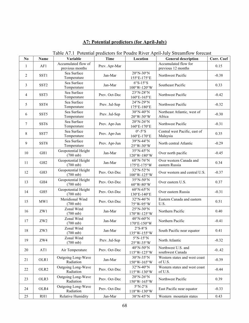
68

A7: Potential predictors (for April-July)

Table A7.1 Potential predictors for Poudre River April-July Streamflow forecast No Name Variable Time Location General description Corr. Coef

1 AF1 Accumulated flow of

previous months Prev. Apr-Mar

Accumulated flow for

previous 12 months 0.15

2 SST1 Sea Surface

Temperature Jan-Mar

20°N-30°N

155°E-175°E Northwest Pacific -0.38

3 SST2 Sea Surface

Temperature Jan-Mar

6°S-15°S

100°W-120°W Southeast Pacific 0.33

4 SST3 Sea Surface

Temperature Prev. Oct-Dec

23°N-28°N

160°E-165°E Northwest Pacific -0.42

5 SST4 Sea Surface

Temperature Prev. Jul-Sep

24°N-29°N

175°E-180°E Northwest Pacific -0.32

6 SST5 Sea Surface

Temperature Prev. Jul-Sep

30°N-40°N

20°W-30°W

Northeast Atlantic, west of

Africa -0.30

7 SST6 Sea Surface

Temperature Prev. Apr-Jun

20°N-26°N

160°E-170°E Northwest Pacific -0.31

8 SST7 Sea Surface

Temperature Prev. Apr-Jun

0°-5°S

160°E-170°E

Central west Pacific, east of

Malaysia 0.35

9 SST8 Sea Surface

Temperature Prev. Apr-Jun

39°N-44°N

25°W-30°W North central Atlantic -0.29

10 GH1 Geopotential Height

(700 mb) Jan-Mar

35°N-45°N

120°W-180°W Over north pacific -0.45

11 GH2 Geopotential Height

(700 mb) Jan-Mar

68°N-76°N

175°E-175°W

Over western Canada and

eastern Russia 0.34

12 GH3 Geopotential Height

(700 mb) Prev. Oct-Dec

32°N-52°N

100°W-125°W Over western and central U.S. -0.37

13 GH4 Geopotential Height

(700 mb) Prev. Oct-Dec

35°N-50°N

60°W-80°W Over eastern U.S. 0.37

14 GH5 Geopotential Height

(700 mb) Prev. Oct-Dec

60°N-65°N

130°E-140°E Over eastern Russia -0.31

15 MW1 Meridional Wind

(700 mb) Prev. Oct-Dec

32°N-46°N

75°W-95°W

Eastern Canada and eastern

U.S. 0.51

16 ZW1 Zonal Wind

(700 mb) Jan-Mar

25°N-30°N

170°W-125°W Northern Pacific 0.40

17 ZW2 Zonal Wind

(700 mb) Jan-Mar

48°N-60°N

170°E-150°W Northern Pacific -0.41

18 ZW3 Zonal Wind

(700 mb) Jan-Mar

2°S-8°S

135°W-155°W South Pacific near equator 0.41

19 ZW4 Zonal Wind

(700 mb) Prev. Jul-Sep

5°N-15°N

25°W-35°W North Atlantic -0.32

20 AT1 Air Temperature Prev. Oct-Dec 40°N-50°N

115°W-125°W

Northwest U.S. and

southwest Canada -0..42

21 OLR1 Outgoing Long-Wave

Radiation Jan-Mar

30°N-35°N

150°W-165°W

Western states and west coast

of U.S. -0.39

22 OLR2 Outgoing Long-Wave

Radiation Prev. Oct-Dec

32°N-40°N

115°W-130°W

Western states and west coast

of U.S. -0.44

23 OLR3 Outgoing Long-Wave

Radiation Prev. Oct-Dec

20°N-26°N

150°W-165°W Northwest Pacific 0.39

24 OLR4 Outgoing Long-Wave

Radiation Prev. Oct-Dec

5°N-2°S

118°W-130°W East Pacific near equator -0.33

25 RH1 Relative Humidity Jan-Mar 38°N-45°N Western mountain states 0.43

69

117°W-122°W

26 RH2 Relative Humidity Jan-Mar 38°N-45°N

85°W-95°W Eastern U.S. 0.42

27 NAO1 North Atlantic

Oscillation Jan 0.34

28 NOI1 Northern Oscillation

Index Jan-Mar -0.42

29 PNA1 Pacific North America

Index Mar 0.38

30 PDO1 Pacific Decadal

Oscillation Mar 0.31

31 SOI1 Southern Oscillation

Index Jan-Mar -0.28

32 PDSI1 Palmer Index Jan-Mar Climate Division 0.32

33 PDSI2 Palmer Index Nov-Dec Climate Division 0.28

34 SWE1 Snow Water

Equivalent Feb 1

st Basin average 0.46

35 SWE2 Snow Water

Equivalent Mar 1

st Basin average 0.49

36 SWE3 Snow Water

Equivalent Apr 1

st Basin average 0.65

Table A7.2 Potential predictors for Arkansas River April-July Flow No Name Variable Time Location General description Corr. Coef

1 AF1 Accumulated flow of

previous months Prev. Apr-Mar

Accumulated flow volumes

for previous 12 months 0.23

2 SST1 Sea Surface

Temperature Jan-Mar

25°N-30°N

160°E-165°E Northwest Pacific -0.46

3 SST2 Sea Surface

Temperature Prev. Oct-Dec

25°N-30°N

160°E-165°E Northwest Pacific -0.39

4 SST3 Sea Surface

Temperature Prev. Jul-Sep

25°N-35°N

20°W-30°W Northwest Atlantic -0.45

5 SST4 Sea Surface

Temperature Prev. Apr-Jun

35°N-45°N

20°W-25°W Northwest Atlantic -0.35

6 GH1 Geopotential Height

(700 mb) Prev. Oct-Dec

38°N-47°N

116°W-122°W Western U.S. -0.39

7 GH2 Geopotential Height

(700 mb) Prev. Oct-Dec

42°N-50°N

70°W-80°W Eastern Canada and U.S. 0.47

8 GH3 Geopotential Height

(700 mb) Prev. Oct-Dec

28°N-33°N

172°E-180°E North central Pacific -0.31

9 MW1 Meridional Wind

(700 mb) Prev. Oct-Dec

45°N-55°N

130°W-135°W Northeast U.S. 0.50

10 MW2 Meridional Wind

(700 mb) Prev. Oct-Dec

35°N-45°N

55°W-60°W

Eastern Canada and eastern

U.S. 0.53

11 ZW1 Zonal Wind

(700 mb) Prev. Oct-Dec

48°N-57°N

105°W-118°W Southern Canada -0.42

12 ZW2 Zonal Wind

(700 mb) Prev. Oct-Dec

27°N-32°N

100°W-118°W Southern U.S. 0.50

13 AT1 Air Temperature Prev. Oct-Dec 35°N-48°N

115°W-130°W Northwest U.S. -0.41

14 OLR1 Outgoing Long-Wave

Radiation Prev. Oct-Dec

40°N-45°N

115°W-120°W

Western mountain states of

U.S. -0.29

15 RH1 Relative Humidity Prev. Oct-Dec 40°N-45°N

117°W-122°W Western mountain states 0.37

16 RH2 Relative Humidity Prev. Oct-Dec 28°N-35°N

75°W-80°W Southeast coast of U.S. 0.49

17 PDSI1 Palmer Index Jan-Mar Climate Division 0.35

18 PDSI2 Palmer Index Prev. Nov-Dec Climate Division 0.28

19 SWE1 Snow Water Feb 1st Basin average 0.56

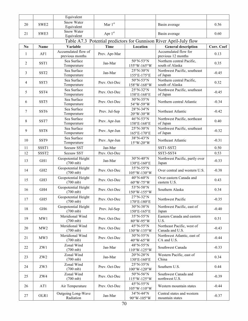
70

Equivalent

20 SWE2 Snow Water

Equivalent Mar 1

st Basin average 0.56

21 SWE3 Snow Water

Equivalent Apr 1

st Basin average 0.60

Table A7.3 Potential predictors for Gunnison River April-July flow No Name Variable Time Location General description Corr. Coef

1 AF1 Accumulated flow of

previous months Prev. Apr-Mar

Accumulated flow for

previous 12 months 0.13

2 SST1 Sea Surface

Temperature Jan-Mar

50°N-53°N

155°W-165°W

Northern central Pacific,

south of Alaska 0.35

3 SST2 Sea Surface

Temperature Jan-Mar

25°N-30°N

155°E-175°E

Northwest Pacific, southeast

of Japan -0.45

4 SST3 Sea Surface

Temperature Prev. Oct-Dec

50°N-53°N

158°W-168°W

Northern central Pacific,

south of Alaska 0.32

5 SST4 Sea Surface

Temperature Prev. Oct-Dec

25°N-32°N

158°E-168°E

Northwest Pacific, southeast

of Japan -0.45

6 SST5 Sea Surface

Temperature Prev. Oct-Dec

30°N-35°N

54°W-59°W Northern central Atlantic -0.34

7 SST6 Sea Surface

Temperature Prev. Jul-Sep

28°N-34°N

20°W-30°W Northeast Atlantic -0.42

8 SST7 Sea Surface

Temperature Prev. Apr-Jun

46°N-53°N

158°E-168°E

Northwest Pacific, northeast

of Japan 0.40

9 SST8 Sea Surface

Temperature Prev. Apr-Jun

25°N-30°N

165°E-170°E

Northwest Pacific, southeast

of Japan -0.32

10 SST9 Sea Surface

Temperature Prev. Apr-Jun

38°N-43°N

15°W-20°W Northeast Atlantic -0.31

11 SSST1 Seesaw SST Jan-Mar SST1-SST2 0.50

12 SSST2 Seesaw SST Prev. Oct-Dec SST3-SST4 0.53

13 GH1 Geopotential Height

(700 mb) Jan-Mar

30°N-40°N

130°E-160°E

Northwest Pacific, partly over

Japan -0.33

14 GH2 Geopotential Height

(700 mb) Prev. Oct-Dec

35°N-55°N

105°W-130°W Over central and western U.S. -0.38

15 GH3 Geopotential Height

(700 mb) Prev. Oct-Dec

40°N-60°N

60°W-75°W

Over eastern Canada and

eastern U.S. 0.43

16 GH4 Geopotential Height

(700 mb) Prev. Oct-Dec

53°N-58°N

150°W-155°W Southern Alaska 0.34

17 GH5 Geopotential Height

(700 mb) Prev. Oct-Dec

27°N-32°N

170°E-180°E Northwest Pacific -0.35

18 GH6 Geopotential Height

(700 mb) Prev. Jul-Sep

30°N-38°N

150°E-165°E

Northwest Pacific, east of

Japan -0.40

19 MW1 Meridional Wind

(700 mb) Prev. Oct-Dec

35°N-55°N

80°W-95°W

Eastern Canada and eastern

U.S. 0.51

20 MW2 Meridional Wind

(700 mb) Prev. Oct-Dec

45°N-55°N

130°W-135°W

Northeast Pacific, west of

Canada and U.S. -0.43

21 MW3 Meridional Wind

(700 mb) Prev. Oct-Dec

30°N-55°N

40°W-65°W

Northwest Atlantic, east of

CA and U.S. -0.44

22 ZW1 Zonal Wind

(700 mb) Jan-Mar

48°N-55°N

110°W-125°W Southwest Canada -0.33

23 ZW2 Zonal Wind

(700 mb) Jan-Mar

20°N-28°N

130°E-160°E

Western Pacific, east of

China 0.34

24 ZW3 Zonal Wind

(700 mb) Prev. Oct-Dec

25°N-35°N

100°W-120°W Southern U.S. 0.44

25 ZW4 Zonal Wind

(700 mb) Prev. Oct-Dec

50°N-56°N

115°W-125°W

Southwest Canada and

northwest U.S. -0.39

26 AT1 Air Temperature Prev. Oct-Dec 45°N-55°N

105°W-110°W Western mountain states -0.44

27 OLR1 Outgoing Long-Wave

Radiation Jan-Mar

34°N-44°N

90°W-105°W

Central states and western

mountain states -0.37

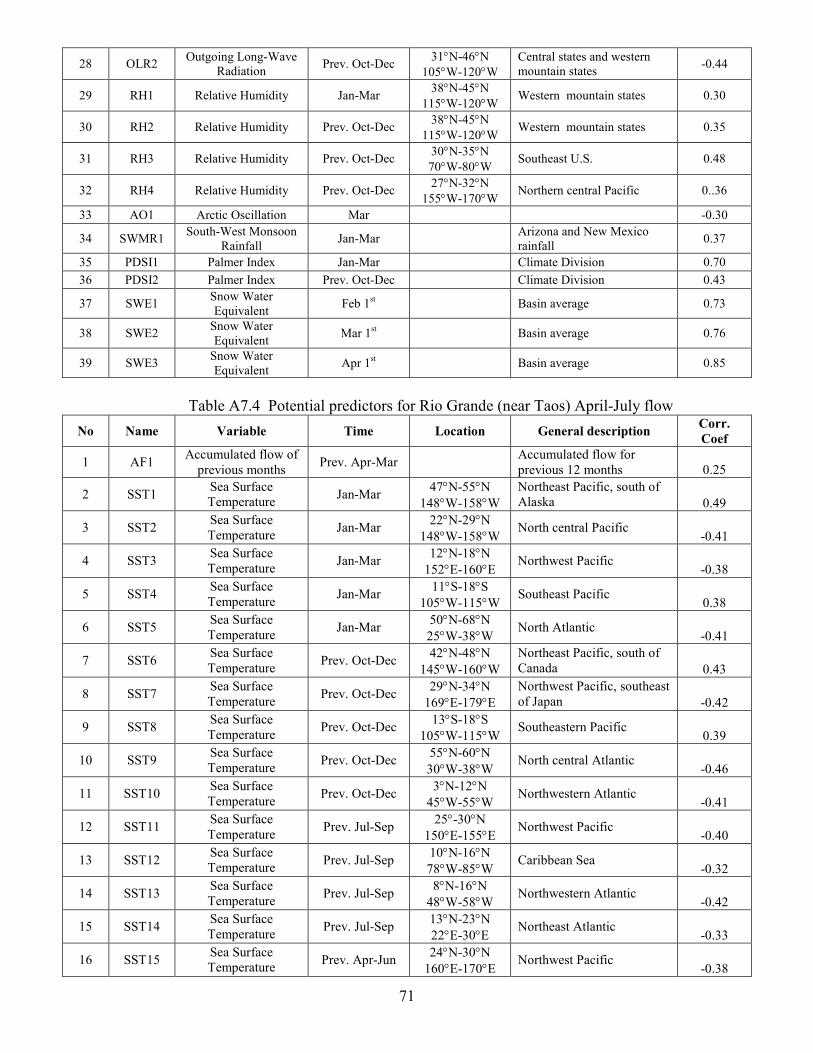
71

28 OLR2 Outgoing Long-Wave

Radiation Prev. Oct-Dec

31°N-46°N

105°W-120°W

Central states and western

mountain states -0.44

29 RH1 Relative Humidity Jan-Mar 38°N-45°N

115°W-120°W Western mountain states 0.30

30 RH2 Relative Humidity Prev. Oct-Dec 38°N-45°N

115°W-120°W Western mountain states 0.35

31 RH3 Relative Humidity Prev. Oct-Dec 30°N-35°N

70°W-80°W Southeast U.S. 0.48

32 RH4 Relative Humidity Prev. Oct-Dec 27°N-32°N

155°W-170°W Northern central Pacific 0..36

33 AO1 Arctic Oscillation Mar -0.30

34 SWMR1 South-West Monsoon

Rainfall Jan-Mar

Arizona and New Mexico

rainfall 0.37

35 PDSI1 Palmer Index Jan-Mar Climate Division 0.70

36 PDSI2 Palmer Index Prev. Oct-Dec Climate Division 0.43

37 SWE1 Snow Water

Equivalent Feb 1

st Basin average 0.73

38 SWE2 Snow Water

Equivalent Mar 1

st Basin average 0.76

39 SWE3 Snow Water

Equivalent Apr 1

st Basin average 0.85

Table A7.4 Potential predictors for Rio Grande (near Taos) April-July flow

No Name Variable Time Location General description Corr.

Coef

1 AF1 Accumulated flow of

previous months Prev. Apr-Mar

Accumulated flow for

previous 12 months 0.25

2 SST1 Sea Surface

Temperature Jan-Mar

47°N-55°N

148°W-158°W

Northeast Pacific, south of

Alaska 0.49

3 SST2 Sea Surface

Temperature Jan-Mar

22°N-29°N

148°W-158°W North central Pacific

-0.41

4 SST3 Sea Surface

Temperature Jan-Mar

12°N-18°N

152°E-160°E Northwest Pacific

-0.38

5 SST4 Sea Surface

Temperature Jan-Mar

11°S-18°S

105°W-115°W Southeast Pacific

0.38

6 SST5 Sea Surface

Temperature Jan-Mar

50°N-68°N

25°W-38°W North Atlantic

-0.41

7 SST6 Sea Surface

Temperature Prev. Oct-Dec

42°N-48°N

145°W-160°W

Northeast Pacific, south of

Canada 0.43

8 SST7 Sea Surface

Temperature Prev. Oct-Dec

29°N-34°N

169°E-179°E

Northwest Pacific, southeast

of Japan -0.42

9 SST8 Sea Surface

Temperature Prev. Oct-Dec

13°S-18°S

105°W-115°W Southeastern Pacific

0.39

10 SST9 Sea Surface

Temperature Prev. Oct-Dec

55°N-60°N

30°W-38°W North central Atlantic

-0.46

11 SST10 Sea Surface

Temperature Prev. Oct-Dec

3°N-12°N

45°W-55°W Northwestern Atlantic

-0.41

12 SST11 Sea Surface

Temperature Prev. Jul-Sep

25°-30°N

150°E-155°E Northwest Pacific

-0.40

13 SST12 Sea Surface

Temperature Prev. Jul-Sep

10°N-16°N

78°W-85°W Caribbean Sea

-0.32

14 SST13 Sea Surface

Temperature Prev. Jul-Sep

8°N-16°N

48°W-58°W Northwestern Atlantic

-0.42

15 SST14 Sea Surface

Temperature Prev. Jul-Sep

13°N-23°N

22°E-30°E Northeast Atlantic

-0.33

16 SST15 Sea Surface

Temperature Prev. Apr-Jun

24°N-30°N

160°E-170°E Northwest Pacific

-0.38

72

17 SST16 Sea Surface

Temperature Prev. Apr-Jun

52°N-59°N

25°W-35°W North Atlantic

-0.45

18 SST17 Sea Surface

Temperature Prev. Apr-Jun

35°N-45°N

10°W-20°W Northeast Atlantic

-0.45

19 SSST1 Seesaw SST Jan-Mar SST1-SST2 0.54

20 SSST2 Seesaw SST Prev. Oct-Dec SST6-SST7 0.52

21 GH1 Geopotential Height

(700 mb) Jan-Mar

29°N-39°N

120°W-130°W West coast of U.S.

-0.39

22 GH2 Geopotential Height

(700 mb) Prev. Oct-Dec

30°N-40°N

110°W-120°W Southwest U.S.

-0.46

23 GH3 Geopotential Height

(700 mb) Prev. Oct-Dec

28°N-38°N

70°W-80°W Southeast U.S.

0.61

24 GH4 Geopotential Height

(700 mb) Prev. Oct-Dec

46°N-56°N

140°W-150°W Northeast Pacific

0.50

25 GH5 Geopotential Height

(700 mb) Prev. Oct-Dec

60°N-70°N

90°W-105°W Northeast Canada

-0.44

26 GH6 Geopotential Height

(700 mb) Prev. Oct-Dec

52°N-62°N

28°W-38°W Northern Atlantic

-0.51

27 GH7 Geopotential Height

(700 mb) Prev. Jul-Sep

30°N-40°N

160°E-170°E Northwest Pacific

-0.35

28 MW1 Meridional Wind

(700 mb) Prev. Oct-Dec

44°N-54°N

132°W-124°W

Northwestern U.S. and

southwest coast of Canada -0.57

29 MW2 Meridional Wind

(700 mb) Prev. Oct-Dec

28°N-44°N

80°W-100°W Eastern U.S.

0.61

30 MW3 Meridional Wind

(700 mb) Prev. Oct-Dec

44°N-50°N

50°W-60°W East coast of Canada

-0.52

31 ZW1 Zonal Wind

(700 mb) Jan-Mar

40°N-50°N

108°W-122°W Northwest U.S.

-0.45

32 ZW2 Zonal Wind

(700 mb) Jan-Mar

20°N-30°N

110°W-120°W

Northeastern Pacific, west

of Mexico 0.46

33 ZW3 Zonal Wind

(700 mb) Prev. Oct-Dec

20°N-30°N

100°W-120°W South of U.S.

0.61

34 ZW4 Zonal Wind

(700 mb) Prev. Oct-Dec

22°N-28°N

60°W-85°W Caribbean Sea

-0.47

35 ZW5 Zonal Wind

(700 mb) Prev. Jul-Sep

7°N-15°N

50°W-58°W Northwest Atlantic

-0.45

36 ZW6 Zonal Wind

(700 mb) Prev. Jul-Sep

22°N-30°N

35°W-60°W Central north Atlantic

0.41

37 AT1 Air Temperature Prev. Oct-Dec 32°N-50°N

105°W-120°W Western U.S.

-0.67

38 OLR1 Outgoing Long-Wave

Radiation Jan-Mar

32°N-40°N

105°W-115°W Southwestern U.S.

-0.49

39 OLR2 Outgoing Long-Wave

Radiation Prev. Oct-Dec

30°N-42°N

100°W-112°W Southwestern U.S.

-0.61

40 RH1 Relative Humidity Jan-Mar 33°N-40°N

105°W-115°W Southwestern U.S.

0.53

41 RH2 Relative Humidity Prev. Oct-Dec 30°N-40°N

105°W-118°W Southwestern U.S.

0.60

42 RH3 Relative Humidity Prev. Oct-Dec 32°N-40°N

89°W-109°W Central east U.S.

0.59

43 PDO1 Pacific Decadal

Oscillation Mar

0.40

44 PDSI1 Palmer Index Jan-Mar Climate Division 0.51

45 PDSI2 Palmer Index Prev. Nov-Dec Climate Division 0.36

46 SWE1 Snow Water

Equivalent Feb 1

st Basin average

0.46

73

47 SWE2 Snow Water

Equivalent Mar 1

st Basin average

0.49

48 SWE3 Snow Water

Equivalent Apr 1

st Basin average

0.65

Table A7.5 Potential predictors for San Juan River April-July flow No Name Variable Time Location General description Corr. Coef

1 AF1 Accumulated flow of

previous months Prev. Apr-Mar

Accumulated flow of

previous 12 months -0.08

2 SST1 Sea Surface

Temperature Jan-Mar

40°N-50°N

145°W-155°W Northeast Pacific 0.40

3 SST2 Sea Surface

Temperature Jan-Mar

12°S-20°S

105°W-115°W Southeast Pacific 0.32

4 SST3 Sea Surface

Temperature Prev. Oct-Dec

42°N-48°N

160°W-170°W

North central Pacific, south

of Alaska 0.31

5 SST4 Sea Surface

Temperature Prev. Oct-Dec

28°N-33°N

170°E-175°E

Northwest Pacific, southeast

of Japan -0.48

6 SST5 Sea Surface

Temperature Prev. Jul-Sep

18°N-30°N

20°W-25°W North central Atlantic -0.43

7 SST6 Sea Surface

Temperature Prev. Apr-Jun

25°N-30°N

150°E-170°E Northwest Pacific -0.35

8 SST7 Sea Surface

Temperature Prev. Apr-Jun

30°N-46°N

15°W-20°W Northeast Atlantic -0.41

9 GH1 Geopotential Height

(700 mb) Jan-Mar

30°N-35°N

115°W-125°W West coast of U.S. -0.59

10 GH2 Geopotential Height

(700 mb) Prev. Oct-Dec

30°N-35°N

110°W-120°W Southwest U.S. -0.46

11 GH3 Geopotential Height

(700 mb) Prev. Oct-Dec

31°N-36°N

70°W-75°W Southeast U.S. 0.40

12 GH4 Geopotential Height

(700 mb) Prev. Oct-Dec

45°N-55°N

145°W-150°W Northeast Pacific 0.42

13 GH5 Geopotential Height

(700 mb) Prev. Oct-Dec

28°N-33°N

175°E-180°E North central Pacific -0.42

14 MW1 Meridional Wind

(700 mb) Prev. Oct-Dec

32°N-45°N

80°W-92°W Eastern U.S. 0.49

15 MW2 Meridional Wind

(700 mb) Prev. Oct-Dec

33°N-45°N

120°W-128°W West coast of U.S. -0.50

16 MW3 Meridional Wind

(700 mb) Prev. Oct-Dec

45°N-50°N

50°W-60°W Northwest Atlantic -0.40

17 ZW1 Zonal Wind

(700 mb) Jan-Mar

45°N-50°N

110°W-120°W Northern U.S. -0.43

18 ZW2 Zonal Wind

(700 mb) Jan-Mar

22°N-29°N

115°W-122°W Northeast Pacific 0.54

19 ZW3 Zonal Wind

(700 mb) Prev. Oct-Dec

22°N-29°N

115°W-122°W Northeast Pacific 0.50

20 AT1 Air Temperature Prev. Oct-Dec 35°N-46°N

115°W-120°W Western U.S. -0.54

21 AT2 Air Temperature Prev. Oct-Dec 28°N-33°N

80°W-85°W Southeast U.S. 0.38

22 OLR1 Outgoing Long-Wave

Radiation Jan-Mar

33°N-40°N

110°W-115°W Central U.S. -0.58

23 OLR2 Outgoing Long-Wave

Radiation Prev. Oct-Dec

33°N-40°N

110°W-115°W Central U.S. -0.48

24 RH1 Relative Humidity Jan-Mar 28°N-33°N

110°W-115°W Southwest U.S. 0.57

25 RH2 Relative Humidity Prev. Oct-Dec 28°N-33°N

110°W-115°W Southwest U.S. 0.48

26 NOI1 Northern Oscillation

Index Jan-Mar -0.31

27 SWMR1 Southwest Monsoon Jan-Mar Arizona and New Mexico 0.60

74

Rainfall rainfall

28 PDSI1 Palmer Index Jan-Mar Climate Division 0.64

29 PDSI2 Palmer Index Prev. Nov-Dec Climate Division 0.38

30 SWE1 Snow Water

Equivalent Feb 1

st Basin average 0.62

31 SWE2 Snow Water

Equivalent Mar 1

st Basin average 0.67

32 SWE3 Snow Water

Equivalent Apr 1

st Basin average 0.85

Table A7.6 Potential predictors for Yampa River April-July flow No Name Variable Time Location General description Corr. Coef

1 AF1 Accumulated flow of

previous months Prev. Apr-Mar

Accumulated flow for

previous 12 months 0.22

2 SST1 Sea Surface

Temperature Jan-Mar

45°N-50°N

170°W-175°W

Northern central Pacific,

south of Alaska 0.42

3 SST2 Sea Surface

Temperature Jan-Mar

25°N-30°N

160°E-165°E

Northwest Pacific, southeast

of Japan -0.52

4 SST3 Sea Surface

Temperature Prev. Jul-Sep

29°N-34°N

20°W-30°W Northeast Atlantic -0.45

5 SST4 Sea Surface

Temperature Prev. Apr-Jun

30°N-35°N

170°W-180°W Northern central Pacific -0.37

6 GH1 Geopotential Height

(700 mb) Jan-Mar

30°N-35°N

155°E-160°E Northwest Pacific -0.43

7 GH2 Geopotential Height

(700 mb) Prev. Oct-Dec

35°N-50°N

100°W-120°W Northern U.S. -0.53

8 GH3 Geopotential Height

(700 mb) Prev. Oct-Dec

53°N-58°N

60°W-65°W Eastern Canada 0.38

9 MW1 Meridional Wind

(700 mb) Prev. Oct-Dec

45°N-55°N

85°W-95°W

Eastern Canada and eastern

U.S. 0.54

10 MW2 Meridional Wind

(700 mb) Prev. Oct-Dec

45°N-56°N

135°W-145°W West coast of Canada -0.43

11 MW3 Meridional Wind

(700 mb) Prev. Oct-Dec

35°N-45°N

57°W-62°W Northwest Atlantic -0.41

12 ZW1 Zonal Wind

(700 mb) Jan-Mar

31°N-36°N

115°W-120°W West coast of U.S. 0.42

13 ZW2 Zonal Wind

(700 mb) Jan-Mar

52°N-57°N

115°W-120°W Southern Canada -0.36

14 ZW3 Zonal Wind

(700 mb) Jan-Mar

22°N-28°N

150°E-160°E Northwest Pacific 0.41

15 ZW4 Zonal Wind

(700 mb) Jan-Mar

42°N-48°N

155°E-165°E Northwest Pacific -0.38

16 ZW5 Zonal Wind

(700 mb) Prev. Oct-Dec

30°N-35°N

105°W-120°W Southern U.S. 0.56

17 ZW6 Zonal Wind

(700 mb) Prev. Oct-Dec

55°N-60°N

110°W-122°W Southern Canada -0.52

18 AT1 Air Temperature Prev. Oct-Dec 48°N-55°N

110°W-122°W Western Canada -0.56

19 OLR1 Outgoing Long-Wave

Radiation Jan-Mar

33°N-38°N

116°W-121°W Southwest U.S. -0.34

20 OLR2 Outgoing Long-Wave

Radiation Jan-Mar

38°N-43°N

90°W-100°W Eastern U.S. -0.38

21 OLR3 Outgoing Long-Wave

Radiation Prev. Oct-Dec

33°N-40°N

115°W-120°W Southwest U.S. -0.49

22 RH1 Relative Humidity Jan-Mar 33°N-38°N

115°W-120°W Western U.S. 0.35

23 RH2 Relative Humidity Jan-Mar 32°N-37°N

87°W-92°W Southeast U.S. 0.37

75

24 RH3 Relative Humidity Prev. Oct-Dec 33°N-38°N

115°W-120°W Western U.S. 0.36

25 PDO1 Pacific Decadal

Oscillation Mar 0.30

26 SWMR1 South-West Monsoon

Rainfall Jan

Arizona and New Mexico

rainfall 0.30

27 PDSI1 Palmer Index Jan-Mar Climate Division 0.66

28 PDSI2 Palmer Index Prev. Nov-Dec Climate Division 0.40

29 SWE1 Snow Water

Equivalent Feb 1

st Basin average 0.54

30 SWE2 Snow Water

Equivalent Mar 1

st Basin average 0.57

31 SWE3 Snow Water

Equivalent Apr 1

st Basin average 0.51

A8: Potential predictors for yearly

Table A8.1 Potential predictors for Poudre River April-March flow No Name Variable Time Location General description Corr. Coef

1 Log-1 Lag-1 flow Prev. Apr-Mar 0.20

2 SST1 Sea Surface

Temperature Jan-Mar

20°N-28°N

160°E-170°E Northwest Pacific -0.42

3 SST2 Sea Surface

Temperature Jan-Mar

5°S-15°S

110°W-120°W Southeast Pacific 0.33

4 SST3 Sea Surface

Temperature Oct-Dec

24°N-30°N

160°E-170°E Northwest Pacific -0.43

5 SST4 Sea Surface

Temperature Oct-Dec

5°S-20°S

85°W-110°W Southeast Pacific 0.30

6 SST5 Sea Surface

Temperature Jul-Sep

23°N-29°N

172°E-180°W Northwest Pacific -0.33

7 SST6 Sea Surface

Temperature Jul-Sep

30°N-36°N

22°W-30°W Northeast Atlantic -0.35

8 SST7 Sea Surface

Temperature Apr-Jun

20°N-25°N

160°E-170°E Northwest Pacific -0.33

9 SST8 Sea Surface

Temperature Apr-Jun

33°N-38°N

25°W-30°W Northeast Atlantic -0.29

10 SSST1 Seesaw SST Jan-Mar SST2 – SST1 0.52

11 SSST2 Seesaw SST Oct-Dec SST4 – SST3 0.46

12 GH1 Geopotential Height

(700 mb) Jan-Mar

32°N-45°N

170°E-150°W North Pacific -0.41

13 GH2 Geopotential Height

(700 mb) Oct-Dec

40°N-50°N

105°W-120°W West U.S. -0.38

14 GH3 Geopotential Height

(700 mb) Oct-Dec

40°N-50°N

60°W-70°W East U.S. 0.38

15 GH4 Geopotential Height

(700 mb) Jul-Sep

15°N-20°N

25°W-32°W East Atlantic 0.30

16 MW1 Meridional Wind

(700 mb) Jan-Mar

14°N-19°N

120°W-125°W Northeast Pacific -0.44

17 MW2 Meridional Wind

(700 mb) Oct-Dec

35°N-45°N

80°E-90°W

Northwest U.S. and

southwest Canada 0.52

18 ZW1 Zonal Wind

(700 mb) Jan-Mar

50°N-60°N

170°E-180°E Northwest Pacific -0.45

19 ZW2 Zonal Wind

(700 mb) Jan-Mar

25°N-30°N

170°E-175°W Central north Pacific 0.33

20 ZW3 Zonal Wind

(700 mb) Oct-Dec

53°N-58°N

108°W-120°W South Canada -0.38

21 ZW4 Zonal Wind

(700 mb) Jul-Sep

5°N-15°N

25°W-40°W Northeast Atlantic -0.34

76

22 AT1 Air Temperature Oct-Dec 42°N-55°N

110°W-125°W

Northwest U.S. and

southwest Canada -0.45

23 AT2 Air Temperature Jul-Sep 58°N-65°N

30°W-45°W South Greenland -0.38

24 OLR1 Outgoing Long-Wave

Radiation Oct-Dec

33°N-45°S

110°W-125°W West U.S. -0.45

25 RH1 Relative Humidity Jan-Mar 35°N-40°N

90°W-95°W Central U.S. 0.47

26 EA1 East Atlantic

Oscillation Jun 0.38

27 MEI1 Multivariate ENSO

Index Mar 0.31

28 NAO1 North Atlantic

Oscillation Jan 0.34

29 NOI1 Northern Oscillation

Index Jan-Mar -0.42

30 PDO1 Pacific Decadal

Oscillation Mar 0.33

31 PNA1 Pacific North

American Index Mar 0.35

32 PNA2 Pacific North

American Index Oct-Dec -0.33

33 SOI1 Southern Oscillation

Index Feb -0.32

34 SWM1 Southwest Monsoon

Rainfall Jan-Mar 0.36

35 PDSI1 Palmer Index Mar Climate Division 0.48

36 PDSI2 Palmer Index Feb Climate Division 0.37

37 PDSI3 Palmer Index Jan Climate Division 0.36

38 SWE Snow Water

Equivalent Feb 1

st Basin average 0.49

39 SWE Snow Water

Equivalent Mar 1

st Basin average 0.44

40 SWE Snow Water

Equivalent Apr 1

st Basin average 0.63

Table A8.2 Potential predictors for Poudre River October-September flow No Name Variable Time Location General description Corr. Coef

1 Lag-1 Lag-1 flow Prev. Oct-Sep 0.16

2 SST1 Sea Surface

Temperature Jul-Sep

23°N-28°N

172°E-179°E Central North Pacific -0.37

3 SST2 Sea Surface

Temperature Jul-Sep

25°N-30°N

85°W-90°W

Southeast Pacific, west of

Peru 0.31

4 SST3 Sea Surface

Temperature Jul-Sep

30°N-35°N

14°W-28°W Northeast Atlantic -0.33

5 SST4 Sea Surface

Temperature Apr-Jun

22°N-29°N

172°W-179°W Central North Pacific -0.33

6 SST5 Sea Surface

Temperature Apr-Jun

32°N-38°N

21°W-32°W Northeast Atlantic -0.35

7 SST6 Sea Surface

Temperature Jan-Mar

31°N-36°N

69°W-74°W Northeast Atlantic -0.29

8 SST7 Sea Surface

Temperature Oct-Dec

31°N-38°N

55°W-62°W Northeast Atlantic -0.32

9 GH1 Geopotential Height

(700 mb) Jul-Sep

12°N-20°N

20°W-30°W Northeast Atlantic 0.31

10 GH2 Geopotential Height

(700 mb) Apr-Jun

44°N-50°N

120°W-1130°W

Northwest U.S. and

southwest Canada 0.30

11 GH3 Geopotential Height

(700 mb) Apr-Jun

1°N-6°N

22°W-30°W North Atlantic near equator 0.29

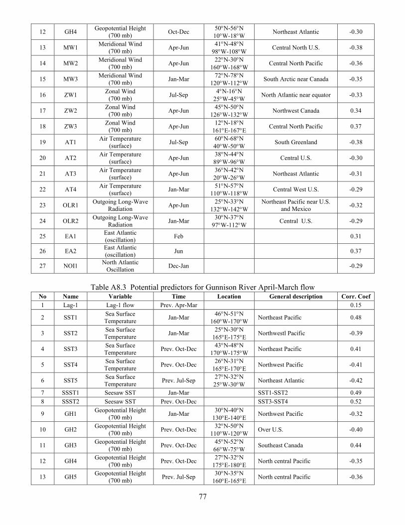
77

12 GH4 Geopotential Height

(700 mb) Oct-Dec

50°N-56°N

10°W-18°W Northeast Atlantic -0.30

13 MW1 Meridional Wind

(700 mb) Apr-Jun

41°N-48°N

98°W-108°W Central North U.S. -0.38

14 MW2 Meridional Wind

(700 mb) Apr-Jun

22°N-30°N

160°W-168°W Central North Pacific -0.36

15 MW3 Meridional Wind

(700 mb) Jan-Mar

72°N-78°N

120°W-112°W South Arctic near Canada -0.35

16 ZW1 Zonal Wind

(700 mb) Jul-Sep

4°N-16°N

25°W-45°W North Atlantic near equator -0.33

17 ZW2 Zonal Wind

(700 mb) Apr-Jun

45°N-50°N

126°W-132°W Northwest Canada 0.34

18 ZW3 Zonal Wind

(700 mb) Apr-Jun

12°N-18°N

161°E-167°E Central North Pacific 0.37

19 AT1 Air Temperature

(surface) Jul-Sep

60°N-68°N

40°W-50°W South Greenland -0.38

20 AT2 Air Temperature

(surface) Apr-Jun

38°N-44°N

89°W-96°W Central U.S. -0.30

21 AT3 Air Temperature

(surface) Apr-Jun

36°N-42°N

20°W-26°W Northeast Atlantic -0.31

22 AT4 Air Temperature

(surface) Jan-Mar

51°N-57°N

110°W-118°W Central West U.S. -0.29

23 OLR1 Outgoing Long-Wave

Radiation Apr-Jun

25°N-33°N

132°W-142°W

Northeast Pacific near U.S.

and Mexico -0.32

24 OLR2 Outgoing Long-Wave

Radiation Jan-Mar

30°N-37°N

97°W-112°W Central U.S. -0.29

25 EA1 East Atlantic

(oscillation) Feb 0.31

26 EA2 East Atlantic

(oscillation) Jun 0.37

27 NOI1 North Atlantic

Oscillation Dec-Jan -0.29

Table A8.3 Potential predictors for Gunnison River April-March flow No Name Variable Time Location General description Corr. Coef

1 Lag-1 Lag-1 flow Prev. Apr-Mar 0.15

2 SST1 Sea Surface

Temperature Jan-Mar

46°N-51°N

160°W-170°W Northeast Pacific 0.48

3 SST2 Sea Surface

Temperature Jan-Mar

25°N-30°N

165°E-175°E Northwestl Pacific -0.39

4 SST3 Sea Surface

Temperature Prev. Oct-Dec

43°N-48°N

170°W-175°W Northeast Pacific 0.41

5 SST4 Sea Surface

Temperature Prev. Oct-Dec

26°N-31°N

165°E-170°E Northwest Pacific -0.41

6 SST5 Sea Surface

Temperature Prev. Jul-Sep

27°N-32°N

25°W-30°W Northeast Atlantic -0.42

7 SSST1 Seesaw SST Jan-Mar SST1-SST2 0.49

8 SSST2 Seesaw SST Prev. Oct-Dec SST3-SST4 0.52

9 GH1 Geopotential Height

(700 mb) Jan-Mar

30°N-40°N

130°E-140°E Northwest Pacific -0.32

10 GH2 Geopotential Height

(700 mb) Prev. Oct-Dec

32°N-50°N

110°W-120°W Over U.S. -0.40

11 GH3 Geopotential Height

(700 mb) Prev. Oct-Dec

45°N-52°N

66°W-75°W Southeast Canada 0.44

12 GH4 Geopotential Height

(700 mb) Prev. Oct-Dec

27°N-32°N

175°E-180°E North central Pacific -0.35

13 GH5 Geopotential Height

(700 mb) Prev. Jul-Sep

30°N-35°N

160°E-165°E North central Pacific -0.36

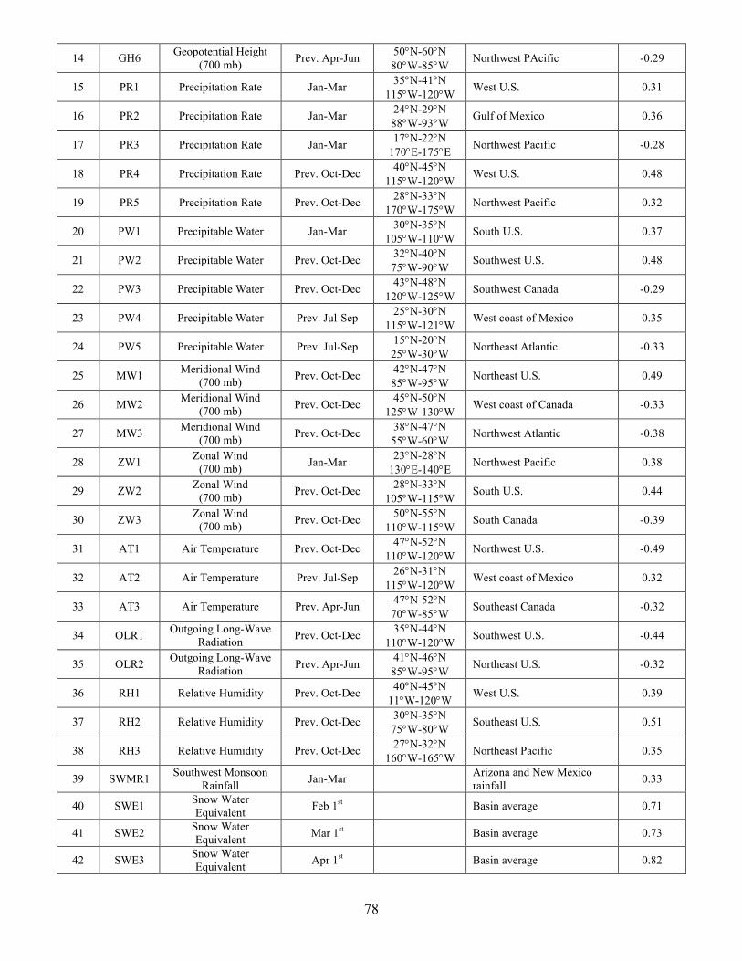
78

14 GH6 Geopotential Height

(700 mb) Prev. Apr-Jun

50°N-60°N

80°W-85°W Northwest PAcific -0.29

15 PR1 Precipitation Rate Jan-Mar 35°N-41°N

115°W-120°W West U.S. 0.31

16 PR2 Precipitation Rate Jan-Mar 24°N-29°N

88°W-93°W Gulf of Mexico 0.36

17 PR3 Precipitation Rate Jan-Mar 17°N-22°N

170°E-175°E Northwest Pacific -0.28

18 PR4 Precipitation Rate Prev. Oct-Dec 40°N-45°N

115°W-120°W West U.S. 0.48

19 PR5 Precipitation Rate Prev. Oct-Dec 28°N-33°N

170°W-175°W Northwest Pacific 0.32

20 PW1 Precipitable Water Jan-Mar 30°N-35°N

105°W-110°W South U.S. 0.37

21 PW2 Precipitable Water Prev. Oct-Dec 32°N-40°N

75°W-90°W Southwest U.S. 0.48

22 PW3 Precipitable Water Prev. Oct-Dec 43°N-48°N

120°W-125°W Southwest Canada -0.29

23 PW4 Precipitable Water Prev. Jul-Sep 25°N-30°N

115°W-121°W West coast of Mexico 0.35

24 PW5 Precipitable Water Prev. Jul-Sep 15°N-20°N

25°W-30°W Northeast Atlantic -0.33

25 MW1 Meridional Wind

(700 mb) Prev. Oct-Dec

42°N-47°N

85°W-95°W Northeast U.S. 0.49

26 MW2 Meridional Wind

(700 mb) Prev. Oct-Dec

45°N-50°N

125°W-130°W West coast of Canada -0.33

27 MW3 Meridional Wind

(700 mb) Prev. Oct-Dec

38°N-47°N

55°W-60°W Northwest Atlantic -0.38

28 ZW1 Zonal Wind

(700 mb) Jan-Mar

23°N-28°N

130°E-140°E Northwest Pacific 0.38

29 ZW2 Zonal Wind

(700 mb) Prev. Oct-Dec

28°N-33°N

105°W-115°W South U.S. 0.44

30 ZW3 Zonal Wind

(700 mb) Prev. Oct-Dec

50°N-55°N

110°W-115°W South Canada -0.39

31 AT1 Air Temperature Prev. Oct-Dec 47°N-52°N

110°W-120°W Northwest U.S. -0.49

32 AT2 Air Temperature Prev. Jul-Sep 26°N-31°N

115°W-120°W West coast of Mexico 0.32

33 AT3 Air Temperature Prev. Apr-Jun 47°N-52°N

70°W-85°W Southeast Canada -0.32

34 OLR1 Outgoing Long-Wave

Radiation Prev. Oct-Dec

35°N-44°N

110°W-120°W Southwest U.S. -0.44

35 OLR2 Outgoing Long-Wave

Radiation Prev. Apr-Jun

41°N-46°N

85°W-95°W Northeast U.S. -0.32

36 RH1 Relative Humidity Prev. Oct-Dec 40°N-45°N

11°W-120°W West U.S. 0.39

37 RH2 Relative Humidity Prev. Oct-Dec 30°N-35°N

75°W-80°W Southeast U.S. 0.51

38 RH3 Relative Humidity Prev. Oct-Dec 27°N-32°N

160°W-165°W Northeast Pacific 0.35

39 SWMR1 Southwest Monsoon

Rainfall Jan-Mar

Arizona and New Mexico

rainfall 0.33

40 SWE1 Snow Water

Equivalent Feb 1

st Basin average 0.71

41 SWE2 Snow Water

Equivalent Mar 1

st Basin average 0.73

42 SWE3 Snow Water

Equivalent Apr 1

st Basin average 0.82

79

Table A8.4 Potential predictors for Gunnison River October-September flow No Name Variable Time Location General description Corr. Coef

1 Lag-1 Lag-1 flow Prev. Oct-Sep 0.15

2 SST1 Sea Surface

Temperature Jul-Sep

35°N-40°N

155°E-175°E

North-west Pacific, east of

Japan -0.34

3 SST2 Sea Surface

Temperature Jul-Sep

11°S-16°S

85°W-115°W

South-east Pacific, west of

Peru 0.28

4 SST3 Sea Surface

Temperature Apr-Jun

35°N-40°N

155°E-160°E

North-west Pacific, east of

Japan -0.35

5 SST4 Sea Surface

Temperature Apr-Jun

31°N-36°N

45°W-55°W

Central northern Atlantic,

east of U.S. -0.38

6 SST5 Sea Surface

Temperature Jan-Mar

47°N-52°N

165°W-170°W

North-east Pacific, south of

Alaska 0.51

7 SST6 Sea Surface

Temperature Jan-Mar

21°N-26°N

155°E-165°E

North-west Pacific, east of

Japan -0.41

8 SSST1 Seesaw SST Jul-Sep SST1-SST2 0.36

9 SSST2 Seesaw SST Jan-Mar SST5-SST6 0.52

10 GH1 Geopotential Height

(700 mb) Jul-Sep

35°N-45°N

160°E-175°E

North-west Pacific, east of

Japan -0.35

11 GH2 Geopotential Height

(700 mb) Jul-Sep

28°N-35°N

50°W-60°W Northern central Atlantic -0.29

12 GH3 Geopotential Height

(700 mb) Apr-Jun

27°N-32°N

95°W-105°W Southern states -0.40

13 GH4 Geopotential Height

(700 mb) Apr-Jun

30°N-40°N

40°W-60°W Northern central Atlantic -0.35

14 GH5 Geopotential Height

(1000 mb) Jul-Sep

55°N-65°N

57°W-105°W Eastern Canada -0.31

15 GH6 Geopotential Height

(1000 mb) Jul-Sep

25°N-30°N

120°E-130°E Western Pacific near China 0.32

16 GH7 Geopotential Height

(1000 mb) Apr-Jun

25°N-35°N

50°W-60°W Northern central Atlantic -0.40

17 PR1 Precipitation Rate Jan-Mar 17°N-22°N

165°E-175°E

Western Pacific, north of

Marshall Islands -0.30

18 MW1 Meridional Wind

(700 mb) Jul-Sep

28°N-35°N

150°E-155°E

Western Pacific, south-east of

Japan -0.45

19 MW2 Meridional Wind

(700 mb) Apr-Jun

25°N-28°N

110°W-118°W

East Pacific, near CA and

Mexico -0.37

20 MW3 Meridional Wind

(surface) Jul-Sep

25°N-31°N

150°E-155°E Western Pacific, east of Japan -0.34

21 ZW1 Zonal Wind

(700 mb) Jul-Sep

48°N-53°N

170°E-175°E

North-west Pacific, north-east

of Japan -0.28

22 ZW2 Zonal Wind

(700 mb) Jul-Sep

27°N-32°N

160°E-165°E Western Pacific, east of Japan 0.43

23 ZW3 Zonal Wind

(700 mb) Jul-Sep

49°N-54°N

28°W-35°W

Central northern Atlantic,

east of Canada -0.29

24 AT1 Air Temperature Jul-Sep 41°N-46°N

105°W-110°W Western mountain states -0.28

25 AT2 Air Temperature Apr-Jun 35°N-40°N

100°W-105°W Western mountain states -0.42

26 OLR1 Outgoing Long-Wave

Radiation Apr-Jun

35°N-45°N

90°W-110°W

Central states and western

mountain states -0.43

27 AO1 Arctic Oscillation Mar-May -0.38

28 PDO1 Pacific Decadal

Oscillation Mar 0.29

29 PDO2 Pacific Decadal

Oscillation Sep 0.28

30 PNA1

Pacific/ North

American

Teleconnection Pattern

Mar-Apr 0.38

80

31 SWM1 South-West Monsoon

Rainfall Jan-Mar

Arizona and New Mexico

rainfall 0.33

31 SWE4 Snow Water

Equivalent May 1

st Basin average 0.33

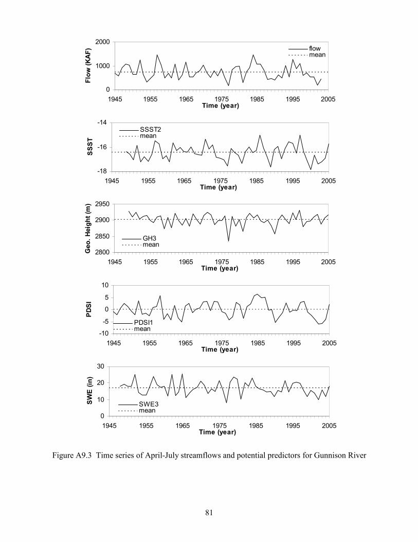
81

0

1000

2000

1945 1955 1965 1975 1985 1995 2005Time (year)

Flow (KAF) flow

mean

-18

-16

-14

1945 1955 1965 1975 1985 1995 2005Time (year)

SSST

SSST2mean

2800

2850

2900

2950

1945 1955 1965 1975 1985 1995 2005Time (year)

Geo. Height (m

)

GH3mean

-10

-5

0

5

10

1945 1955 1965 1975 1985 1995 2005Time (year)

PDSI

PDSI1mean

0

10

20

30

1945 1955 1965 1975 1985 1995 2005Time (year)

SWE (in)

SWE3mean

Figure A9.3 Time series of April-July streamflows and potential predictors for Gunnison River

82

0

200

400

600

800

24 25 26 27 28

SST (C)

Flow (KAF)

SST3 vs flow

0

200

400

600

800

2850 2900 2950 3000 3050

Geopotential Height (m)

Flow (KAF)

GH1 vs flow

(a) (b)

0

200

400

600

800

-3 -2 -1 0 1 2 3

Meridional w ind

Flow (KAF)

MW1 vs flow

0

200

400

600

800

0 5 10 15 20 25 30

SWE (in)

Flow (KAF)

SWE3 vs flow

(c) (d)

Figure A9.7 Potential predictor for Poudre River April-July streamflow: (a) SST3, (b) GH1, (c)

MW1, and (d) SWE3

0

200

400

600

800

20 20.5 21 21.5 22 22.5

SST (C)

Flow (KAF)

SST1 vs f low

0

200

400

600

800

2850 2880 2910 2940 2970 3000

Geopotential Height (m)

Flow (KAF)

GH2 vs f low

(a) (b)

0

200

400

600

800

-2 0 2 4 6

Precip Rate

Flow (KAF)

MW2 vs f low

0

200

400

600

800

0 5 10 15 20

SWE (in)

Flow (KAF)

SWE3 vs flow

(c) (d)

Figure A9.8 Potential predictor for Arkansas River April-July streamflow: (a) SST1, (b) GH2,

(c) MW2, and (d) SWE3

83

0

500

1000

1500

2000

-18 -17 -16 -15 -14

SSST

Flow (KAF)

SSST2 vs f low

0

500

1000

1500

2000

2820 2840 2860 2880 2900 2920 2940

Geopotential Height (m)

Flow (KAF)

GH3 vs flow

(a) (b)

0

500

1000

1500

2000

-8 -4 0 4 8

PDSI

Flow (KAF)

PDSI1 vs flow

0

500

1000

1500

2000

0 5 10 15 20 25 30

SWE (in)

Flow (KAF)

SWE3 vs f low

(c) (d)

Figure A9.9 Potential predictor vs. Gunnison River April-July streamflow: (a) SSST2, (b) GH3,

(c) PDSI1, and (d) SWE3

0

300

600

900

1200

-18 -16 -14 -12 -10

SSST

Flow (KAF)

SSST1 vs f low

0

300

600

900

1200

0 1 2 3 4 5 6 7

Zonal w ind

Flow (KAF)

ZW3 vs flow

(a) (b)

0

300

600

900

1200

3050 3070 3090 3110 3130 3150

Geopotential Height (m)

Flow (KAF)

GH3 vs flow

0

300

600

900

1200

0 5 10 15 20 25 30 35

SWE (in)

Flow (KAF)

SWE3 vs f low

(c) (d)

Figure A9.10 Potential predictor vs. Rio Grande April-July streamflow: (a) SSST1, (b) ZW3, (c)

GH3, and (d) SWE3

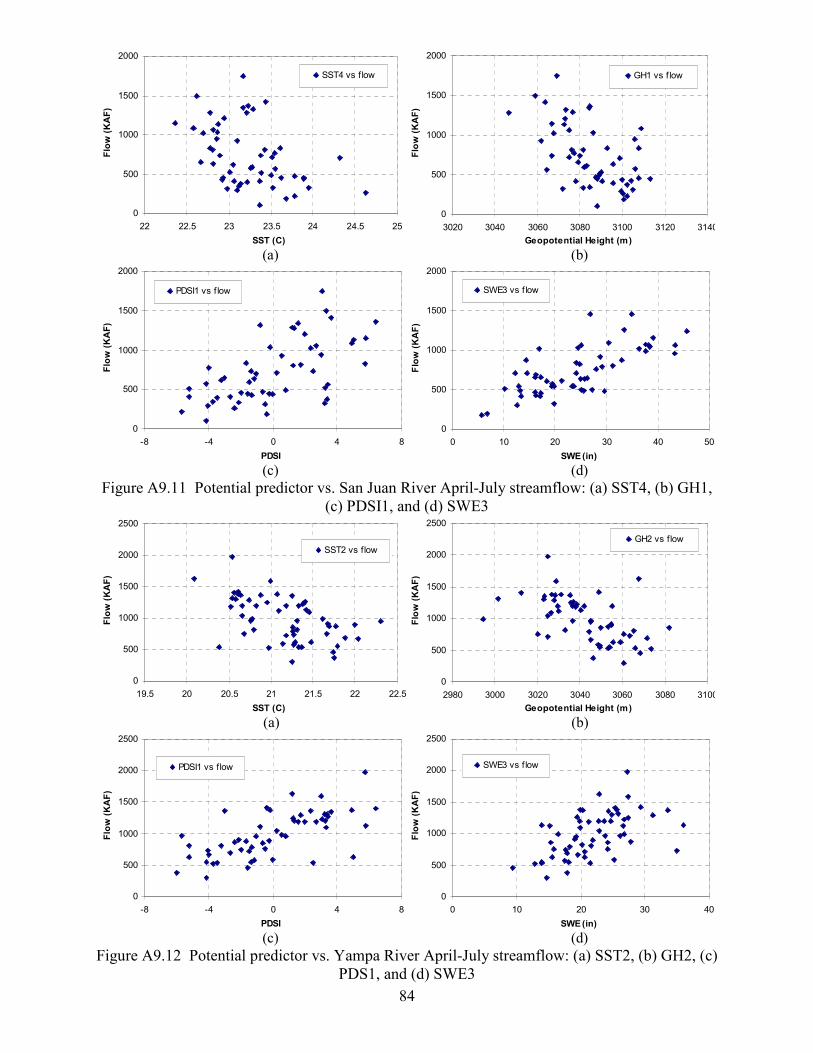
84

0

500

1000

1500

2000

22 22.5 23 23.5 24 24.5 25

SST (C)

Flow (KAF)

SST4 vs f low

0

500

1000

1500

2000

3020 3040 3060 3080 3100 3120 3140

Geopotential Height (m)

Flow (KAF)

GH1 vs f low

(a) (b)

0

500

1000

1500

2000

-8 -4 0 4 8

PDSI

Flow (KAF)

PDSI1 vs f low

0

500

1000

1500

2000

0 10 20 30 40 50

SWE (in)

Flow (KAF)

SWE3 vs f low

(c) (d)

Figure A9.11 Potential predictor vs. San Juan River April-July streamflow: (a) SST4, (b) GH1,

(c) PDSI1, and (d) SWE3

0

500

1000

1500

2000

2500

19.5 20 20.5 21 21.5 22 22.5

SST (C)

Flow (KAF)

SST2 vs flow

0

500

1000

1500

2000

2500

2980 3000 3020 3040 3060 3080 3100

Geopotential Height (m)

Flow (KAF)

GH2 vs flow

(a) (b)

0

500

1000

1500

2000

2500

-8 -4 0 4 8

PDSI

Flow (KAF)

PDSI1 vs flow

0

500

1000

1500

2000

2500

0 10 20 30 40

SWE (in)

Flow (KAF)

SWE3 vs f low

(c) (d)

Figure A9.12 Potential predictor vs. Yampa River April-July streamflow: (a) SST2, (b) GH2, (c)

PDS1, and (d) SWE3

85

Appendix B: Results of PCA and CCA

B1: Results of PCA on the potential predictors for each site

Table B1.1 Variances of PCs for Poudre River

PCs Variance % Accum

% PCs Variance %

Accum

%

1 10.05 27.9 27.9 19 0.31 0.9 95.1

2 4.95 13.7 41.7 20 0.29 0.8 95.9

3 2.66 7.4 49.1 21 0.27 0.7 96.6

4 2.35 6.5 55.6 22 0.24 0.7 97.3

5 2.08 5.8 61.4 23 0.18 0.5 97.8

6 1.70 4.7 66.1 24 0.14 0.4 98.2

7 1.57 4.4 70.4 25 0.13 0.4 98.6

8 1.28 3.6 74.0 26 0.11 0.3 98.9

9 1.17 3.3 77.3 27 0.10 0.3 99.1

10 1.12 3.1 80.4 28 0.08 0.2 99.4

11 0.97 2.7 83.0 29 0.07 0.2 99.5

12 0.76 2.1 85.2 30 0.05 0.1 99.7

13 0.73 2.0 87.2 31 0.04 0.1 99.8

14 0.66 1.8 89.0 32 0.03 0.1 99.9

15 0.55 1.5 90.5 33 0.02 0.1 99.9

16 0.51 1.4 92.0 34 0.01 0.0 100.0

17 0.44 1.2 93.2 35 0.01 0.0 100.0

18 0.38 1.1 94.2 36 0.00 0.0 100.0

Table B1.2 Variances of PCs for Arkansas River

PCs Variance % Accum

% PCs Variance %

Accum

%

1 7.71 36.7 36.7 11 0.29 1.4 94.2

2 2.57 12.2 49.0 12 0.25 1.2 95.4

3 2.26 10.7 59.7 13 0.23 1.1 96.5

4 1.73 8.2 67.9 14 0.19 0.9 97.4

5 1.48 7.0 75.0 15 0.16 0.8 98.2

6 1.10 5.3 80.2 16 0.13 0.6 98.8

7 0.79 3.8 84.0 17 0.10 0.5 99.3

8 0.71 3.4 87.3 18 0.06 0.3 99.5

9 0.64 3.0 90.4 19 0.05 0.2 99.8

10 0.50 2.4 92.8 20 0.03 0.1 99.9

Table B1.3 Variances of PCs for Gunnison River

PCs Variance %

Accum

% PCs Variance %

Accum

%

1 11.50 29.5 29.5 21 0.25 0.6 96.5

2 3.77 9.7 39.2 22 0.23 0.6 97.1

3 3.09 7.9 47.1 23 0.21 0.5 97.7

4 2.77 7.1 54.2 24 0.17 0.4 98.1

5 2.40 6.2 60.3 25 0.14 0.4 98.5

6 2.12 5.4 65.8 26 0.12 0.3 98.8

7 1.69 4.3 70.1 27 0.11 0.3 99.0

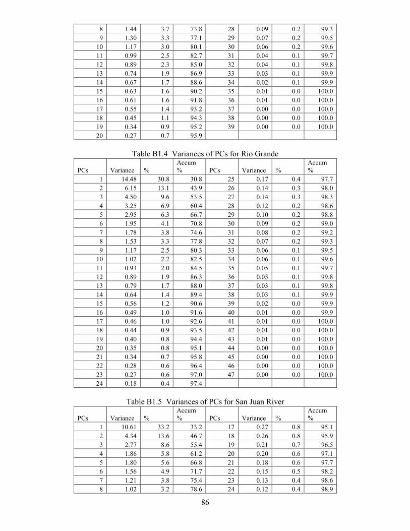
86

8 1.44 3.7 73.8 28 0.09 0.2 99.3

9 1.30 3.3 77.1 29 0.07 0.2 99.5

10 1.17 3.0 80.1 30 0.06 0.2 99.6

11 0.99 2.5 82.7 31 0.04 0.1 99.7

12 0.89 2.3 85.0 32 0.04 0.1 99.8

13 0.74 1.9 86.9 33 0.03 0.1 99.9

14 0.67 1.7 88.6 34 0.02 0.1 99.9

15 0.63 1.6 90.2 35 0.01 0.0 100.0

16 0.61 1.6 91.8 36 0.01 0.0 100.0

17 0.55 1.4 93.2 37 0.00 0.0 100.0

18 0.45 1.1 94.3 38 0.00 0.0 100.0

19 0.34 0.9 95.2 39 0.00 0.0 100.0

20 0.27 0.7 95.9

Table B1.4 Variances of PCs for Rio Grande

PCs Variance %

Accum

% PCs Variance %

Accum

%

1 14.48 30.8 30.8 25 0.17 0.4 97.7

2 6.15 13.1 43.9 26 0.14 0.3 98.0

3 4.50 9.6 53.5 27 0.14 0.3 98.3

4 3.25 6.9 60.4 28 0.12 0.2 98.6

5 2.95 6.3 66.7 29 0.10 0.2 98.8

6 1.95 4.1 70.8 30 0.09 0.2 99.0

7 1.78 3.8 74.6 31 0.08 0.2 99.2

8 1.53 3.3 77.8 32 0.07 0.2 99.3

9 1.17 2.5 80.3 33 0.06 0.1 99.5

10 1.02 2.2 82.5 34 0.06 0.1 99.6

11 0.93 2.0 84.5 35 0.05 0.1 99.7

12 0.89 1.9 86.3 36 0.03 0.1 99.8

13 0.79 1.7 88.0 37 0.03 0.1 99.8

14 0.64 1.4 89.4 38 0.03 0.1 99.9

15 0.56 1.2 90.6 39 0.02 0.0 99.9

16 0.49 1.0 91.6 40 0.01 0.0 99.9

17 0.46 1.0 92.6 41 0.01 0.0 100.0

18 0.44 0.9 93.5 42 0.01 0.0 100.0

19 0.40 0.8 94.4 43 0.01 0.0 100.0

20 0.35 0.8 95.1 44 0.00 0.0 100.0

21 0.34 0.7 95.8 45 0.00 0.0 100.0

22 0.28 0.6 96.4 46 0.00 0.0 100.0

23 0.27 0.6 97.0 47 0.00 0.0 100.0

24 0.18 0.4 97.4

Table B1.5 Variances of PCs for San Juan River

PCs Variance %

Accum

% PCs Variance %

Accum

%

1 10.61 33.2 33.2 17 0.27 0.8 95.1

2 4.34 13.6 46.7 18 0.26 0.8 95.9

3 2.77 8.6 55.4 19 0.21 0.7 96.5

4 1.86 5.8 61.2 20 0.20 0.6 97.1

5 1.80 5.6 66.8 21 0.18 0.6 97.7

6 1.56 4.9 71.7 22 0.15 0.5 98.2

7 1.21 3.8 75.4 23 0.13 0.4 98.6

8 1.02 3.2 78.6 24 0.12 0.4 98.9

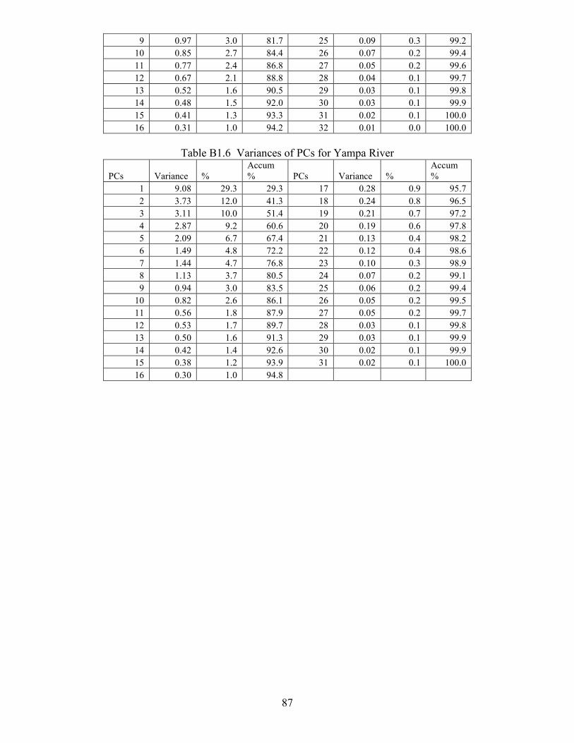
87

9 0.97 3.0 81.7 25 0.09 0.3 99.2

10 0.85 2.7 84.4 26 0.07 0.2 99.4

11 0.77 2.4 86.8 27 0.05 0.2 99.6

12 0.67 2.1 88.8 28 0.04 0.1 99.7

13 0.52 1.6 90.5 29 0.03 0.1 99.8

14 0.48 1.5 92.0 30 0.03 0.1 99.9

15 0.41 1.3 93.3 31 0.02 0.1 100.0

16 0.31 1.0 94.2 32 0.01 0.0 100.0

Table B1.6 Variances of PCs for Yampa River

PCs Variance %

Accum

% PCs Variance %

Accum

%

1 9.08 29.3 29.3 17 0.28 0.9 95.7

2 3.73 12.0 41.3 18 0.24 0.8 96.5

3 3.11 10.0 51.4 19 0.21 0.7 97.2

4 2.87 9.2 60.6 20 0.19 0.6 97.8

5 2.09 6.7 67.4 21 0.13 0.4 98.2

6 1.49 4.8 72.2 22 0.12 0.4 98.6

7 1.44 4.7 76.8 23 0.10 0.3 98.9

8 1.13 3.7 80.5 24 0.07 0.2 99.1

9 0.94 3.0 83.5 25 0.06 0.2 99.4

10 0.82 2.6 86.1 26 0.05 0.2 99.5

11 0.56 1.8 87.9 27 0.05 0.2 99.7

12 0.53 1.7 89.7 28 0.03 0.1 99.8

13 0.50 1.6 91.3 29 0.03 0.1 99.9

14 0.42 1.4 92.6 30 0.02 0.1 99.9

15 0.38 1.2 93.9 31 0.02 0.1 100.0

16 0.30 1.0 94.8

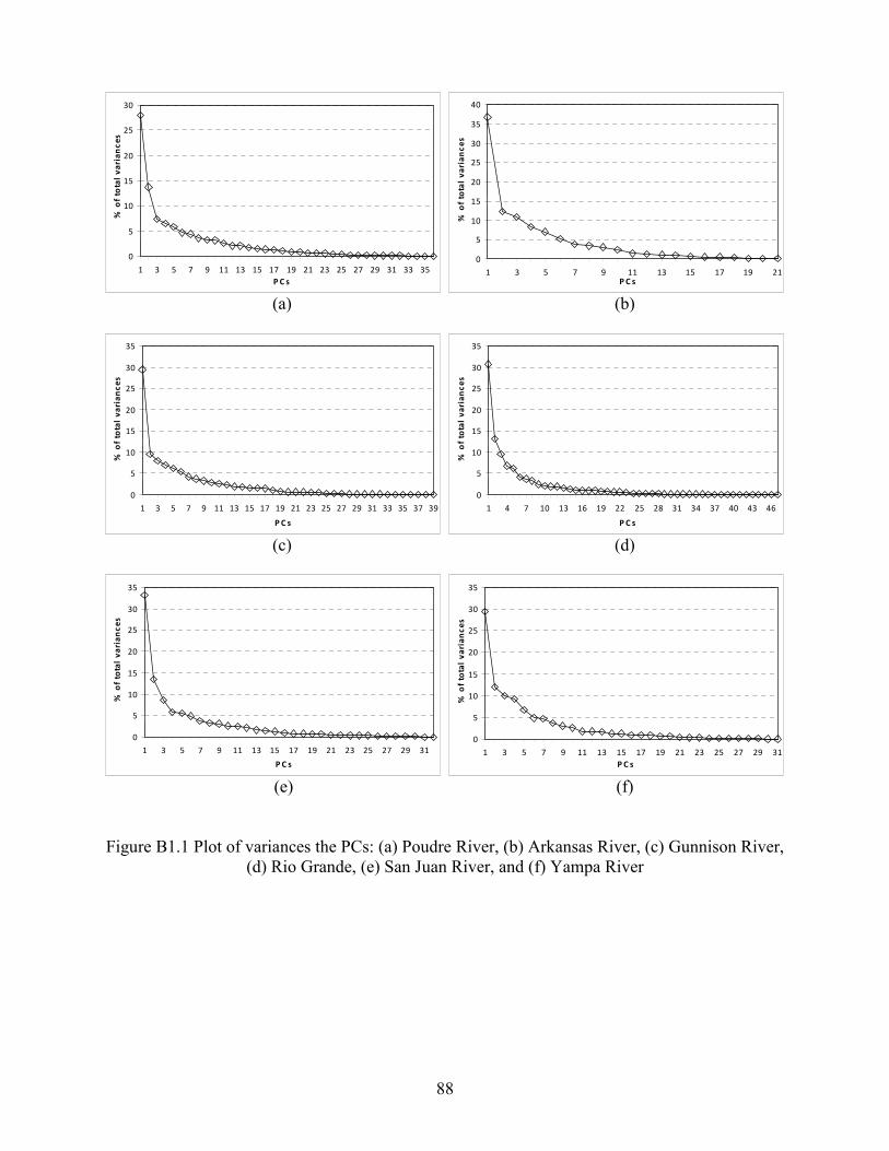
88

0

5

10

15

20

25

30

1 3 5 7 9 11 13 15 17 19 21 23 25 27 29 31 33 35

P C s

% o

f to

tal

va

ria

nc

es

0

5

10

15

20

25

30

35

40

1 3 5 7 9 11 13 15 17 19 21

P C s

% o

f to

tal

va

ria

nc

es

(a) (b)

0

5

10

15

20

25

30

35

1 3 5 7 9 11 13 15 17 19 21 23 25 27 29 31 33 35 37 39

P C s

% o

f to

tal

va

ria

nc

es

0

5

10

15

20

25

30

35

1 4 7 10 13 16 19 22 25 28 31 34 37 40 43 46

P C s

% o

f to

tal

va

ria

nc

es

(c) (d)

0

5

10

15

20

25

30

35

1 3 5 7 9 11 13 15 17 19 21 23 25 27 29 31

P C s

% o

f to

tal

va

ria

nc

es

0

5

10

15

20

25

30

35

1 3 5 7 9 11 13 15 17 19 21 23 25 27 29 31

P C s

% o

f to

tal

va

ria

nc

es

(e) (f)

Figure B1.1 Plot of variances the PCs: (a) Poudre River, (b) Arkansas River, (c) Gunnison River,

(d) Rio Grande, (e) San Juan River, and (f) Yampa River

89

B2: Results of PCA on the potential predictors for all sites

Table B2.1 Variances of PCs obtained from all of the potential predictors for 6 sites

PCs Variance % Accumulated

% PCs Variance %

Accumulated

% PCs Variance %

Accumulated

%

1 51.7 25.1 25.1 26 1.4 0.7 92.5 52 0.2 0.1 100.0

2 23.4 11.4 36.5 27 1.2 0.6 93.1 53 ~ 206 0.0 0.0 100.0

3 15.0 7.3 43.7 28 1.2 0.6 93.7

4 12.1 5.9 49.6 29 1.1 0.5 94.2

5 11.4 5.6 55.2 30 1.0 0.5 94.7

6 9.9 4.8 60.0 31 1.0 0.5 95.2

7 7.8 3.8 63.8 32 1.0 0.5 95.6

8 6.5 3.1 66.9 33 0.9 0.4 96.1

9 5.9 2.9 69.8 34 0.8 0.4 96.5

10 5.1 2.5 72.3 35 0.7 0.4 96.8

11 4.7 2.3 74.5 36 0.7 0.3 97.1

12 4.0 1.9 76.5 37 0.7 0.3 97.5

13 3.8 1.8 78.3 38 0.6 0.3 97.7

14 3.4 1.7 80.0 39 0.6 0.3 98.0

15 3.2 1.6 81.5 40 0.5 0.2 98.3

16 2.9 1.4 83.0 41 0.5 0.2 98.5

17 2.6 1.3 84.2 42 0.4 0.2 98.7

18 2.4 1.2 85.4 43 0.4 0.2 98.9

19 2.3 1.1 86.5 44 0.4 0.2 99.1

20 2.1 1.0 87.5 45 0.3 0.2 99.2

21 2.0 1.0 88.5 46 0.3 0.1 99.4

22 1.9 0.9 89.4 47 0.3 0.1 99.5

23 1.8 0.9 90.3 48 0.3 0.1 99.7

24 1.6 0.8 91.0 49 0.2 0.1 99.8

25 1.6 0.8 91.8 50 0.2 0.1 99.8

0

5

10

15

20

25

30

1 2 3 4 5 6 7 8 9 10 11 12 13 14 15 16 17 18 19 20

PCs

Perc

enta

ge o

f to

tal variance

First 20 PCs

Figure B2.1 Plot of vairance of of the fist 20 PCs obtained fron all of the potential predictors of 6

sites

90

B3: Result of CCA

Table B3.1 a matrix 0.0943 0.0219 0.0473 -0.0237 0.0305 0.015

-0.0339 0.095 0.0022 0.0348 -0.0006 -0.0268

-0.0059 -0.1231 -0.0054 0.0382 0.0242 0.0899

-0.0694 0.0375 0.1038 -0.0223 0.0213 0.0045

-0.0239 0.057 0.0042 -0.0991 -0.0647 0.0586

0.0094 0.0389 -0.1019 0.0784 0.0797 0.0314

-0.0693 0.0175 0.0479 -0.0233 0.1109 0.0484

-0.0342 0.0695 -0.0725 -0.0837 0.0784 0.011

0.1175 0.1079 -0.0199 0.0321 -0.108 0.0313

0.0334 0.0157 -0.0633 0.0597 -0.0203 -0.0009

-0.0332 -0.0073 -0.0945 -0.1367 0.108 -0.06

0.0845 -0.0499 -0.0457 -0.0666 0.0578 -0.0679

0.0111 0.0203 -0.0624 -0.016 0.0729 -0.0859

-0.0414 0.1318 -0.0293 0.0113 0.0957 0.0528

0.03 -0.0718 0.0956 -0.0089 -0.0214 -0.0381

-0.0492 -0.0441 0.0327 -0.0982 -0.0492 -0.1793

0.016 0.0048 -0.0444 0.0244 -0.0885 0.0957

0.0441 0.03 -0.1108 -0.0422 -0.0112 -0.1319

0.0297 0.0052 -0.036 -0.0267 -0.0297 0.0015

-0.014 -0.0798 0.0167 0.0085 -0.1177 -0.127

-0.0113 -0.0161 0.0105 -0.121 -0.0867 -0.1374

-0.0073 -0.049 0.131 0.029 0.031 -0.0988

0.0435 -0.0436 -0.0084 0.1104 -0.0465 -0.177

-0.0309 -0.0239 0.1267 -0.0794 0.0761 0.0368

0.0191 -0.0049 -0.0299 -0.1278 0.0495 -0.0682

-0.083 0.0105 0.1061 0.0228 0.156 -0.0059

-0.0098 -0.0884 -0.0573 0.0753 0.0541 0.0278

-0.0528 -0.0641 -0.042 -0.2432 -0.0046 -0.0196

-0.0418 0.0981 -0.0602 0.0049 -0.0648 0.1066

0.1095 -0.0174 -0.2407 -0.0309 0.1657 -0.0777

0.0728 -0.0798 -0.0507 -0.0073 0.1729 -0.0615

-0.0025 0.065 0.1863 0.3467 0.2018 -0.2754

-0.1306 0.0587 0.0947 0.0177 0.0056 0.0775

0.0747 0.012 -0.0251 0.0727 0.0413 -0.1434

-0.0268 0.0133 0.1342 0.0313 -0.0669 -0.1206

-0.0185 -0.0997 0.0939 -0.0626 0.215 -0.0297

Table B3.2 b matrix

-0.111 0.436 0.052 1.075 -0.168 1.142

0.539 -0.193 0.074 -0.089 -1.385 -1.199

-0.394 -0.815 1.691 1.606 2.031 0.422

-0.414 0.989 -1.010 0.582 0.144 -1.580

-0.586 -0.299 0.677 -1.469 -0.737 1.369

0.095 -0.515 -1.883 -1.453 -0.531 -0.236

91

Appendix C: Model performances

C1: Yearly streamflow forecast models

Table C1.1 Model performance for April – March streamflow forecast of Poudre River

Values of R2 Values of skill scores

Method Item Values Item Values

R2 0.62 Accuracy 0.53

Fitting adj. R

2 0.59 HSS 0.37

R2 0.44 Accuracy 0.51

Drop one adj. R

2 0.39 HSS 0.35

Table C1.2 Model performance for October – September streamflow forecast of Poudre River

Values of R2 Values of skill scores

Method Item Values Item Values

R2 0.65 Accuracy 0.55

Fitting adj. R

2 0.62 HSS 0.40

R2 0.54 Accuracy 0.47

Drop one adj. R

2 0.50 HSS 0.30

92

93

Appendix D: Plot of results

D1: Tim

e series plots for single-site models (M

LR m

odel)

Poudre

Riv

er

0

200

400

600

800

1945

1950

1955

1960

1965

1970

1975

1980

1985

1990

1995

2000

200

5

Years

Flow, TAF

Obs

erv

ed

Fo

reca

st

F

itti

ng

0

200

400

600

800

1945

1950

1955

1960

1965

1970

1975

1980

1985

1990

1995

2000

200

5

Years

Flow, TAF

Ob

se

rve

d

Fo

recas

t

D

rop-1

0%

Fig

. D

1.1

Com

par

ison o

f fo

reca

st r

esult

s fo

r P

oud

re R

iver

Ark

ansa

s R

iver

0

200

400

600

800

1945

1950

1955

1960

1965

1970

1975

1980

1985

1990

1995

2000

200

5

Years

Flow, TAF

Obs

erv

ed

Fo

reca

st

F

itti

ng

0

200

400

600

800

1945

1950

1955

1960

1965

1970

1975

1980

1985

1990

1995

2000

200

5

Years

Flow, TAF

Obse

rve

d

Fo

recas

t

D

rop-1

0%

Fig

. D

1.2

Com

par

ison o

f fo

reca

st r

esult

s fo

r A

rkan

sas

Riv

er

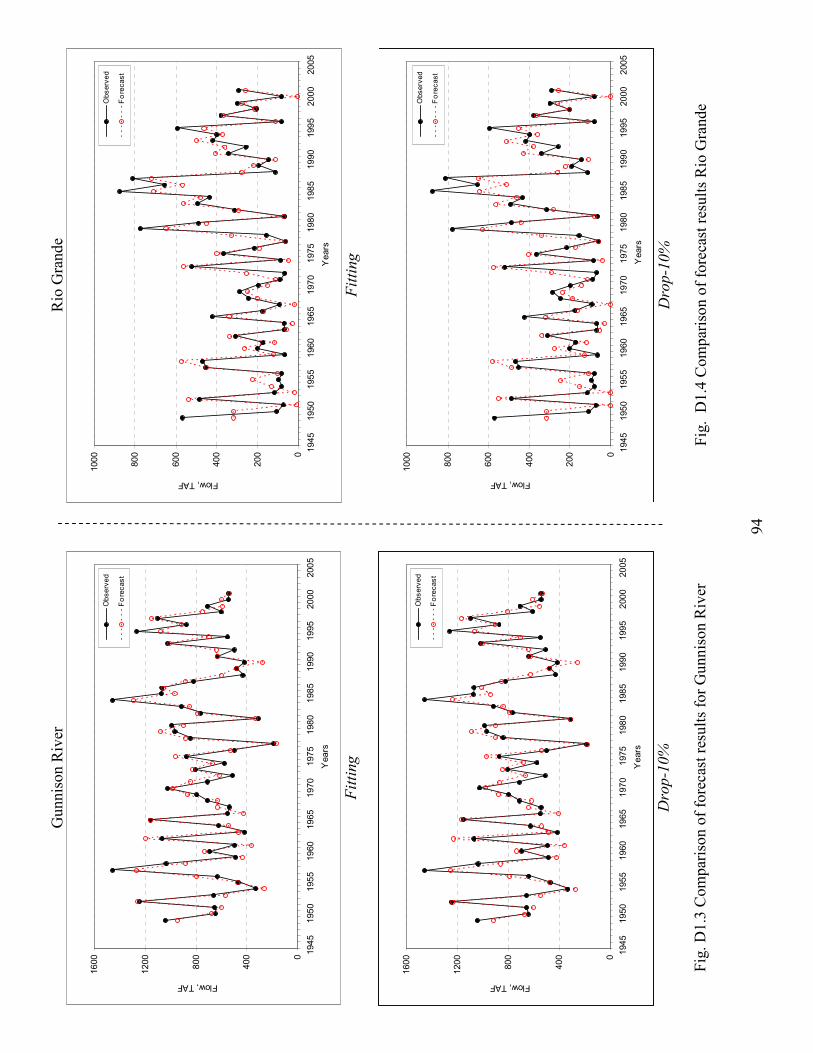
94

Gunnis

on R

iver

0

400

800

1200

1600

1945

1950

1955

1960

1965

1970

1975

1980

1985

1990

1995

2000

200

5

Years

Flow, TAF

Ob

se

rve

d

Fo

rec

as

t

F

itti

ng

0

400

800

1200

1600

1945

1950

1955

1960

1965

1970

1975

1980

1985

1990

1995

2000

2005

Years

Flow, TAF

Obs

erv

ed

Fo

recas

t

D

rop-1

0%

Fig

. D

1.3

Com

par

ison o

f fo

reca

st r

esult

s fo

r G

unn

ison R

iver

Rio

Gra

nde

0

200

400

600

800

1000

1945

1950

1955

1960

1965

1970

1975

1980

1985

1990

1995

2000

2005

Years

Flow, TAF

Obs

erv

ed

Fo

recas

t

F

itti

ng

0

200

400

600

800

10

00

1945

195

0195

519

60

19

65

19

70

1975

1980

198

5199

019

95

20

00

2005

Years

Flow, TAF

Observ

ed

Fo

rec

ast

D

rop-1

0%

Fig

. D

1.4

Com

par

ison o

f fo

reca

st r

esult

s R

io G

rande

95

San

Juan

Riv

er

0

500

10

00

15

00

20

00

1945

195

0195

519

60

19

65

19

70

1975

1980

198

5199

019

95

20

00

2005

Years

Flow, TAF

Observ

ed

Fo

rec

ast

F

itti

ng

0

50

0

100

0

150

0

200

0

19

45

195

0195

51960

1965

1970

1975

19

80

19

85

199

0199

52000

2005

Ye

ars

Flow, TAF

Obse

rved

Fo

recast

D

rop-1

0%

Fig

. D

1.5

Com

par

ison o

f fo

reca

st r

esult

s fo

r S

an J

uan

Riv

er

Yam

pa

Riv

er

0

50

0

100

0

150

0

200

0

250

0

19

45

195

0195

51960

1965

1970

1975

19

80

19

85

199

0199

52000

2005

Ye

ars

Flow, TAF

Obse

rved

Fo

recast

F

itti

ng

0

500

1000

1500

2000

2500

1945

1950

195

51960

1965

19

70

1975

1980

19

85

1990

1995

20

00

2005

Years

Flow, TAF

Ob

serv

ed

Fo

recas

t

D

rop-1

0%

Fig

. D

1.6

Com

par

ison o

f fo

reca

st r

esult

s fo

r Y

ampa

Riv

er

96

D2: Comparison of single –site m

odels (PCA) and CCA m

odel

Sin

gle

-sit

e m

odel

0

200

400

600

800

1945

1950

1955

1960

1965

1970

1975

1980

1985

1990

1995

2000

200

5

Years

Flow, TAF

Obs

erv

ed

Fo

reca

st

F

itti

ng

0

200

400

600

800

19

45

195

019

55

19

60

196

519

70

197

51

98

019

85

199

019

95

20

00

200

5

Yea

rs

Flow, TAF

Ob

se

rve

d

Fo

recas

t

D

rop-1

0%

Fig

. D

2.1

Com

par

ison o

f fo

reca

st r

esult

s fo

r P

oud

re R

iver

Mult

i-si

te -

CC

A

0

200

400

600

800

1945

1950

1955

1960

1965

1970

1975

1980

1985

1990

1995

2000

200

5

Years

Flow, TAF

Observ

ed

Fo

recast

F

itti

ng

0

200

400

600

800

19

45

195

019

55

19

60

196

519

70

197

51

98

019

85

199

019

95

20

00

200

5

Yea

rs

Flow, TAF

Observ

ed

Fo

recast

D

rop-1

0%

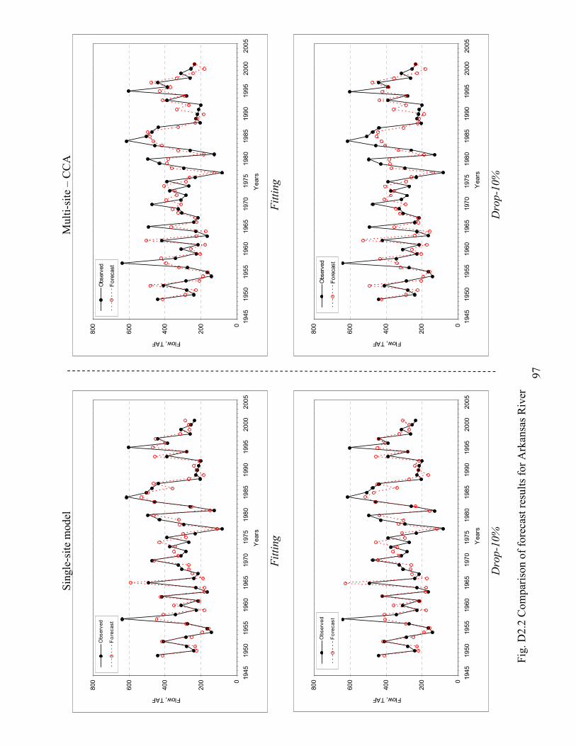
97

Sin

gle

-sit

e m

odel

0

200

400

600

800

19

45

195

019

55

19

60

196

519

70

197

51

98

019

85

199

019

95

20

00

200

5

Ye

ars

Flow, TAF

Obs

erv

ed

Fo

reca

st

F

itti

ng

0

20

0

40

0

60

0

80

0

1945

19

50

19

55

19

60

196

51

97

01

97

51

98

01

985

19

90

19

95

20

00

200

5

Yea

rs

Flow, TAF

Obse

rve

d

Fo

recas

t

D

rop-1

0%

Fig

. D

2.2

Com

par

ison o

f fo

reca

st r

esult

s fo

r A

rkan

sas

Riv

er

Mult

i-si

te –

CC

A

0

200

400

600

800

19

45

195

019

55

19

60

196

519

70

197

51

98

019

85

199

019

95

20

00

200

5

Ye

ars

Flow, TAF

Observ

ed

Fo

recast

F

itti

ng

0

200

400

600

800

1945

1950

1955

1960

1965

1970

1975

1980

1985

1990

1995

2000

2005

Years

Flow, TAF

Observ

ed

Fo

recast

D

rop-1

0%

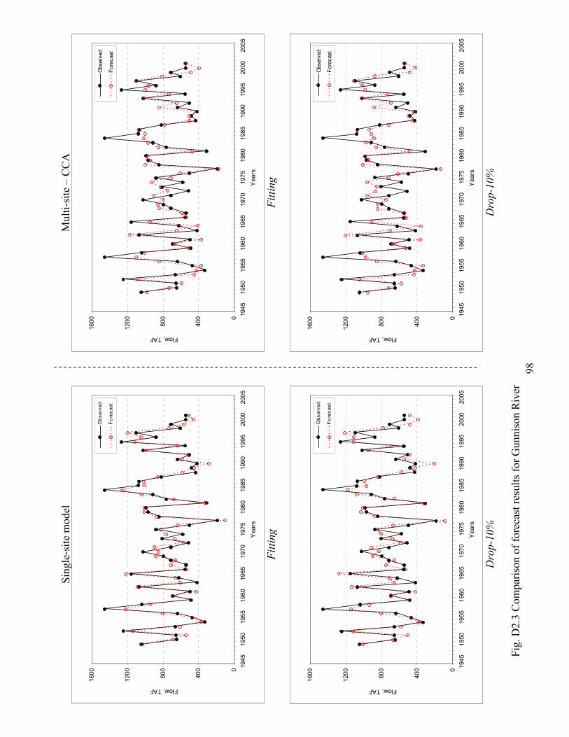
98

Sin

gle

-sit

e m

odel

0

400

800

1200

1600

1945

1950

1955

1960

1965

1970

1975

1980

1985

1990

1995

2000

200

5

Years

Flow, TAF

Ob

se

rve

d

Fo

rec

as

t

F

itti

ng

0

400

800

1200

1600

1945

1950

1955

1960

1965

1970

1975

1980

1985

1990

1995

2000

2005

Years

Flow, TAF

Obs

erv

ed

Fo

recas

t

D

rop-1

0%

Fig

. D

2.3

Com

par

ison o

f fo

reca

st r

esult

s fo

r G

unn

ison R

iver

Mult

i-si

te –

CC

A

0

400

800

1200

1600

1945

1950

1955

1960

1965

1970

1975

1980

1985

1990

1995

2000

2005

Years

Flow, TAF

Observ

ed

Fo

recast

F

itti

ng

0

400

800

1200

1600

1945

1950

1955

1960

1965

1970

1975

1980

1985

1990

1995

2000

2005

Years

Flow, TAF

Observ

ed

Fo

recast

D

rop-1

0%

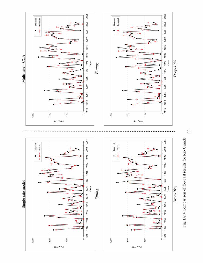
99

Sin

gle

-sit

e m

odel

0

400

800

1200

1945

1950

1955

1960

1965

1970

1975

1980

1985

1990

1995

2000

2005

Years

Flow, TAF

Obs

erv

ed

Fo

recas

t

F

itti

ng

0

400

800

1200

1945

1950

1955

1960

1965

1970

1975

1980

1985

1990

1995

2000

2005

Years

Flow, TAF

Observ

ed

Fo

rec

ast

D

rop-1

0%

Fig

. D

2.4

Com

par

ison o

f fo

reca

st r

esult

s fo

r R

io G

rande

Mult

i-si

te –

CC

A

0

400

800

1200

1945

1950

1955

1960

1965

1970

1975

1980

1985

1990

1995

2000

2005

Years

Flow, TAF

Observ

ed

Fo

recast

F

itti

ng

0

400

800

12

00

1945

195

0195

519

60

19

65

19

70

1975

1980

198

5199

019

95

20

00

20

05

Years

Flow, TAF

Observ

ed

Fo

recast

D

rop-1

0%

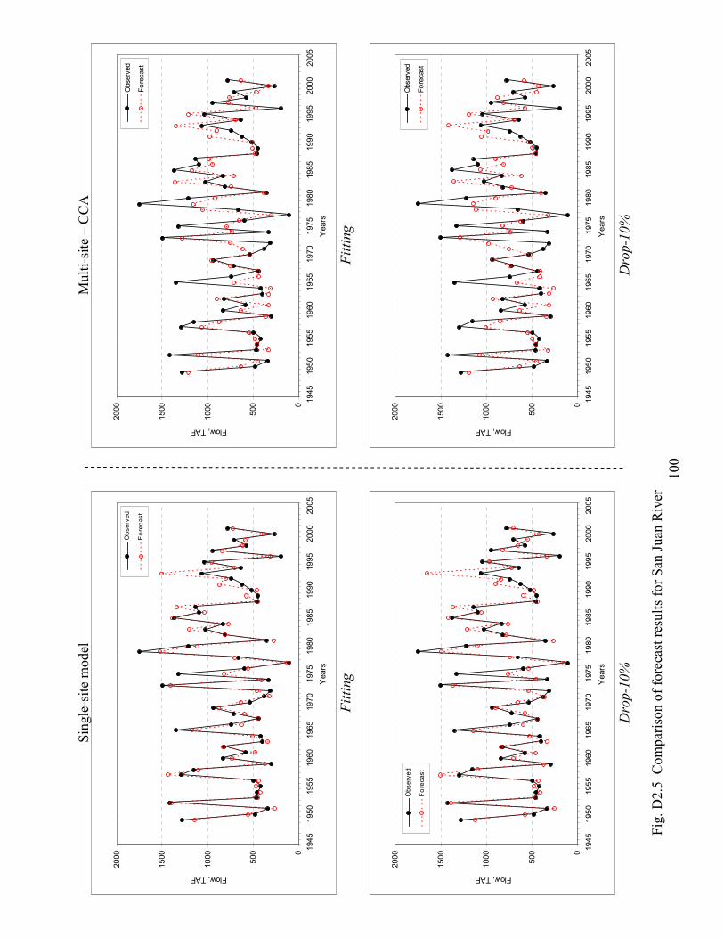
100

Sin

gle

-sit

e m

odel

0

500

10

00

15

00

20

00

1945

195

0195

519

60

19

65

19

70

1975

1980

198

5199

019

95

20

00

2005

Years

Flow, TAF

Observ

ed

Fo

rec

ast

F

itti

ng

0

50

0

100

0

150

0

200

0

19

45

195

0195

51960

1965

1970

1975

19

80

19

85

199

0199

52000

2005

Ye

ars

Flow, TAF

Obse

rved

Fo

recast

D

rop-1

0%

Fig

. D

2.5

C

om

par

ison o

f fo

reca

st r

esult

s fo

r S

an J

uan

Riv

er

Mult

i-si

te –

CC

A

0

500

10

00

15

00

20

00

1945

195

0195

519

60

19

65

19

70

1975

1980

198

5199

019

95

20

00

20

05

Years

Flow, TAF

Observ

ed

Fo

recast

F

itti

ng

0

50

0

100

0

150

0

200

0

19

45

195

0195

51960

1965

1970

1975

19

80

19

85

199

0199

52000

2005

Ye

ars

Flow, TAF

Observ

ed

Fo

recast

D

rop-1

0%

101

Sin

gle

-sit

e m

odel

0

50

0

100

0

150

0

200

0

250

0

19

45

195

0195

51960

1965

1970

1975

19

80

19

85

199

0199

52000

2005

Ye

ars

Flow, TAF

Obse

rved

Fo

recast

F

itti

ng

0

500

1000

1500

2000

2500

1945

1950

195

51960

1965

19

70

1975

1980

19

85

1990

1995

20

00

2005

Years

Flow, TAF

Ob

serv

ed

Fo

recas

t

D

rop-1

0%

Fig

. D

2.6

Com

par

ison o

f fo

reca

st r

esult

s fo

r Y

ampa

Riv

er

Mult

i-si

te –

CC

A

0

50

0

100

0

150

0

200

0

250

0

19

45

195

0195

51960

1965

1970

1975

19

80

19

85

199

0199

52000

2005

Ye

ars

Flow, TAF

Observ

ed

Fo

recast

F

itti

ng

0

500

1000

1500

2000

2500

1945

1950

195

51960

1965

19

70

1975

1980

198

51990

1995

20

00

2005

Years

Flow, TAF

Observ

ed

Fo

recast

D

rop-1

0%

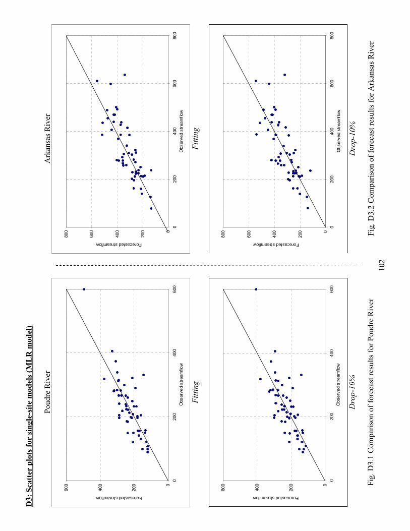
102

D3: Scatter plots for single-site models (M

LR m

odel)

Poudre

Riv

er

0

200

400

600

0200

400

600

Observ

ed s

tream

flow

Forecasted streamflow

F

itti

ng

0

200

400

600

0200

400

600

Observ

ed s

tream

flow

Forecasted streamflow

D

rop-1

0%

Fig

. D

3.1

Com

par

ison o

f fo

reca

st r

esult

s fo

r P

oud

re R

iver

Ark

ansa

s R

iver

0

200

400

600

800

0200

400

600

800

Observ

ed s

tream

flow

Forecasted streamflow

F

itti

ng

0

200

400

600

800

020

040

060

080

0

Obs

erv

ed s

trea

mfl

ow

Forecasted streamflow

D

rop-1

0%

Fig

. D

3.2

Com

par

ison o

f fo

reca

st r

esult

s fo

r A

rkan

sas

Riv

er

103

Gunnis

on R

iver

0

40

0

80

0

120

0

160

0

04

00

80

01

20

01

60

0

Obs

erv

ed s

trea

mfl

ow

Forecasted streamflow

F

itti

ng

0

400

800

12

00

16

00

040

08

00

120

016

00

Obs

erv

ed

str

ea

mfl

ow

Forecasted streamflow

D

rop-1

0%

Fig

. D

3.3

Com

par

ison o

f fo

reca

st r

esult

s fo

r G

unn

ison R

iver

Rio

Gra

nde

0

200

400

600

800

10

00

02

00

40

060

08

00

10

00

Obs

erv

ed

str

ea

mfl

ow

Forecasted streamflow

F

itti

ng

0

20

0

40

0

60

0

80

0

100

0

02

00

400

60

08

00

1000

Ob

se

rve

d s

tre

am

flow

Forecasted streamflow

D

rop-1

0%

Fig

. D

3.4

Com

par

ison o

f fo

reca

st r

esult

s R

io G

ran

de

104

San

Juan

Riv

er

0

50

0

100

0

150

0

200

0

050

0100

01

50

02

000

Ob

se

rve

d s

tre

am

flow

Forecasted streamflow

F

itti

ng

0

500

10

00

15

00

20

00

0500

10

00

1500

200

0

Ob

serv

ed s

tre

am

flow

Forecasted streamflow

D

rop-1

0%

Fig

. D

3.5

Com

par

ison o

f fo

reca

st r

esult

s fo

r S

an J

uan

Riv

er

Yam

pa

Riv

er

0

500

10

00

15

00

20

00

0500

10

00

1500

200

0

Ob

serv

ed s

tre

am

flow

Forecasted streamflow

F

itti

ng

0

50

0

100

0

150

0

200

0

05

00

100

01

500

200

0

Ob

serv

ed s

trea

mflo

w

Forecasted streamflow

D

rop-1

0%

Fig

. D

3.6

. C

om

par

ison o

f fo

reca

st r

esult

s fo

r Y

ampa

Riv

er

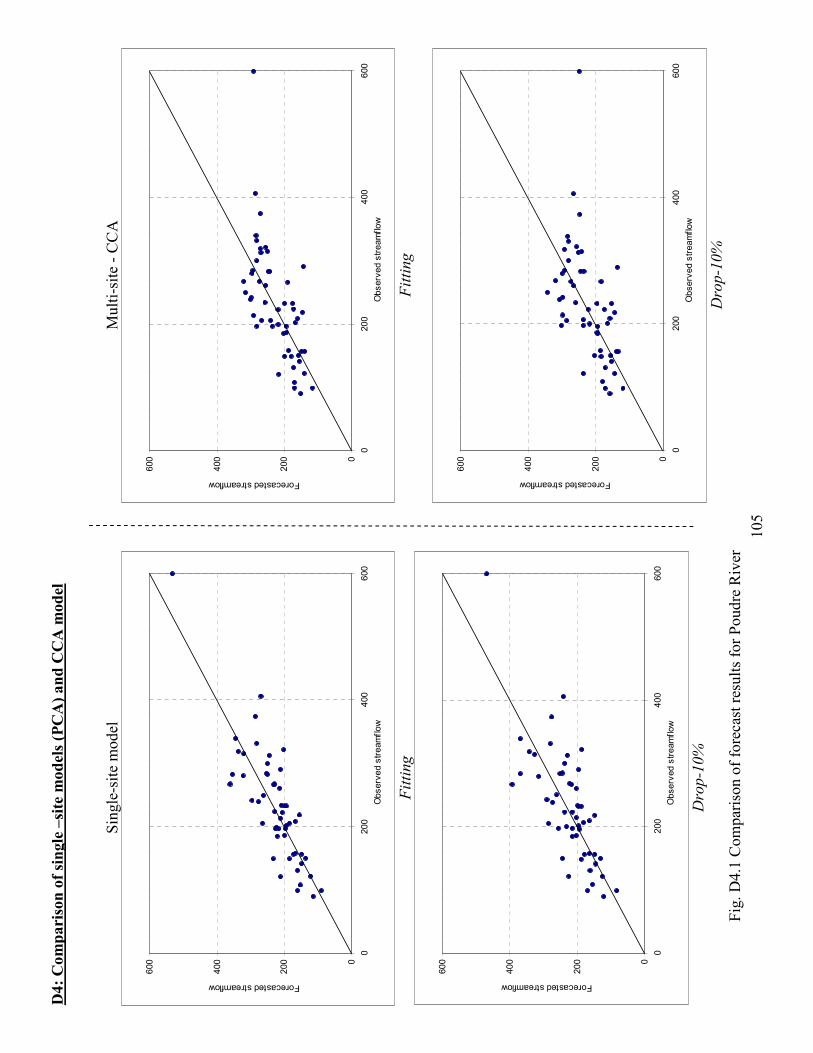
105

D4: Comparison of single –site m

odels (PCA) and CCA m

odel

Sin

gle

-sit

e m

odel

0

200

400

600

0200

400

600

Observ

ed s

tream

flow

Forecasted streamflow

F

itti

ng

0

200

400

600

0200

400

600

Observ

ed s

tream

flow

Forecasted streamflow

D

rop-1

0%

Fig

. D

4.1

Com

par

ison o

f fo

reca

st r

esult

s fo

r P

oud

re R

iver

Mult

i-si

te -

CC

A

0

200

400

600

0200

400

600

Observ

ed s

tream

flow

Forecasted streamflow

F

itti

ng

0

200

400

600

0200

400

600

Observ

ed s

tream

flow

Forecasted streamflow

D

rop-1

0%

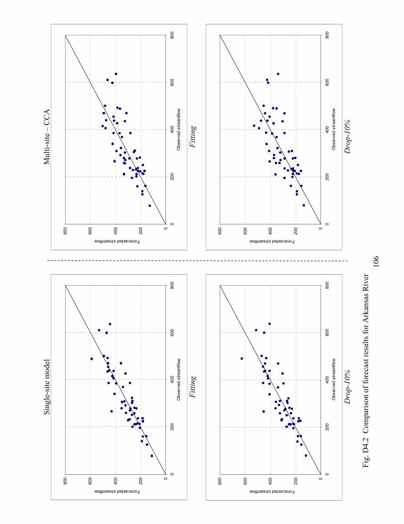
106

Sin

gle

-sit

e m

odel

0

200

400

600

800

0200

400

600

800

Observ

ed s

tream

flow

Forecasted streamflow

F

itti

ng

0

200

400

600

800

020

040

060

080

0

Obs

erv

ed s

trea

mfl

ow

Forecasted streamflow

D

rop-1

0%

Fig

. D

4.2

C

om

par

ison o

f fo

reca

st r

esult

s fo

r A

rkan

sas

Riv

er

Mult

i-si

te –

CC

A

0

200

400

600

800

0200

400

600

800

Observ

ed s

tream

flow

Forecasted streamflow

F

itti

ng

0

200

400

600

800

020

040

060

080

0

Obs

erv

ed s

trea

mfl

ow

Forecasted streamflow

D

rop-1

0%

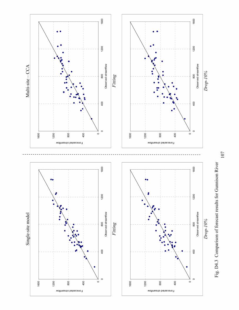
107

Sin

gle

-sit

e m

odel

0

40

0

80

0

120

0

160

0

04

00

80

01

20

01

60

0

Obs

erv

ed s

trea

mfl

ow

Forecasted streamflow

F

itti

ng

0

400

800

12

00

16

00

040

08

00

120

016

00

Obs

erv

ed

str

ea

mfl

ow

Forecasted streamflow

D

rop-1

0%

Fig

. D

4.3

C

om

par

ison o

f fo

reca

st r

esult

s fo

r G

un

nis

on R

iver

Mult

i-si

te –

CC

A

0

40

0

80

0

120

0

160

0

04

00

80

01

20

01

60

0

Obs

erv

ed s

trea

mfl

ow

Forecasted streamflow

F

itti

ng

0

400

800

12

00

16

00

040

08

00

120

016

00

Obs

erv

ed

str

ea

mfl

ow

Forecasted streamflow

D

rop-1

0%

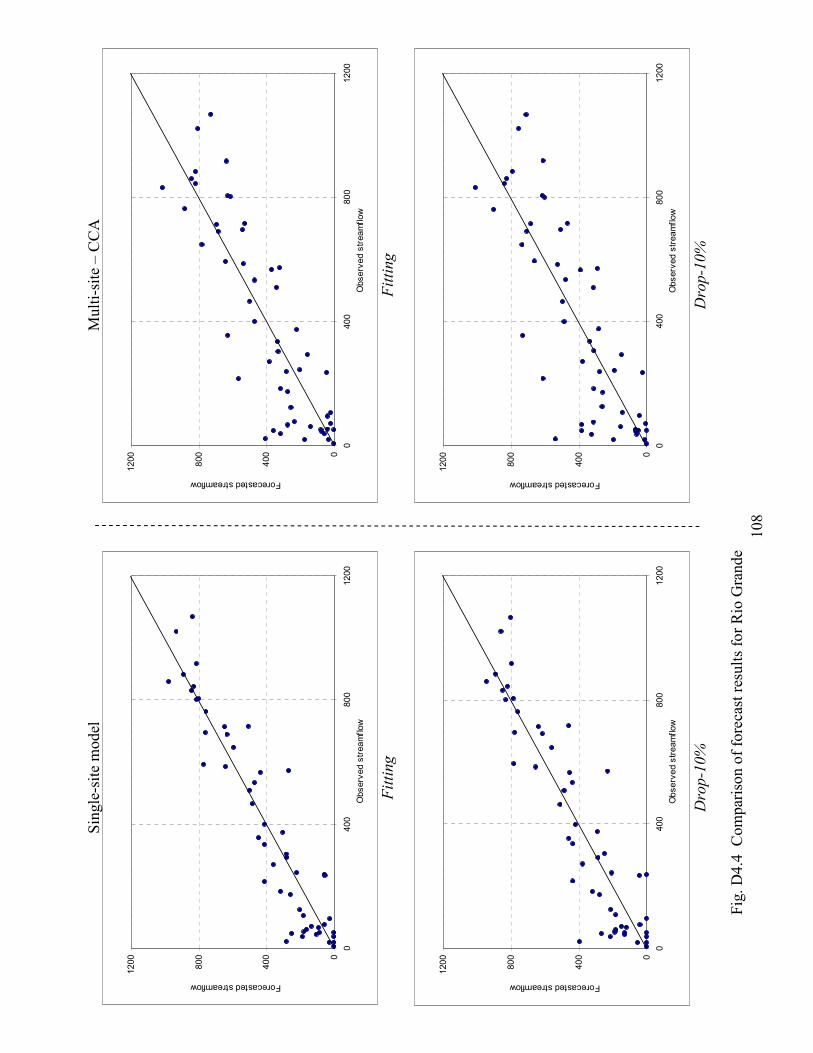
108

Sin

gle

-sit

e m

odel

0

400

800

12

00

040

080

012

00

Obs

erv

ed

str

ea

mfl

ow

Forecasted streamflow

F

itti

ng

0

40

0

80

0

120

0

0400

80

01

200

Ob

se

rve

d s

tre

am

flow

Forecasted streamflow

D

rop-1

0%

Fig

. D

4.4

C

om

par

ison o

f fo

reca

st r

esult

s fo

r R

io G

rande

Mult

i-si

te –

CC

A

0

400

800

12

00

040

080

012

00

Obse

rved s

trea

mfl

ow

Forecasted streamflow

F

itti

ng

0

40

0

80

0

120

0

0400

80

012

00

Obs

erv

ed

str

ea

mfl

ow

Forecasted streamflow

D

rop-1

0%

109

Sin

gle

-sit

e m

odel

0

50

0

100

0

150

0

200

0

050

0100

01

50

02

000

Ob

se

rve

d s

tre

am

flow

Forecasted streamflow

F

itti

ng

0

500

10

00

15

00

20

00

0500

10

00

1500

200

0

Ob

serv

ed s

tre

am

flow

Forecasted streamflow

D

rop-1

0%

Fig

. D

4.5

C

om

par

ison o

f fo

reca

st r

esult

s fo

r S

an J

uan

Riv

er

Mult

i-si

te –

CC

A

0

50

0

100

0

150

0

200

0

050

0100

01

500

20

00

Ob

se

rve

d s

tre

am

flow

Forecasted streamflow

F

itti

ng

0

500

10

00

15

00

20

00

0500

10

00

1500

200

0

Ob

serv

ed s

tre

am

flow

Forecasted streamflow

D

rop-1

0%

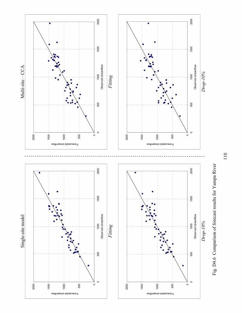
110

Sin

gle

-sit

e m

odel

0

500

10

00

15

00

20

00

0500

10

00

1500

200

0

Ob

serv

ed s

tre

am

flow

Forecasted streamflow

F

itti

ng

0

50

0

100

0

150

0

200

0

05

00

100

01

500

200

0

Ob

serv

ed s

trea

mflo

w

Forecasted streamflow

D

rop-1

0%

Fig

. D

4.6

C

om

par

ison o

f fo

reca

st r

esult

s fo

r Y

ampa

Riv

er

Mult

i-si

te –

CC

A

0

500

10

00

15

00

20

00

0500

10

00

1500

200

0

Ob

serv

ed s

tre

am

flow

Forecasted streamflow

F

itti

ng

0

50

0

100

0

150

0

200

0

0500

100

01

500

20

00

Ob

serv

ed s

trea

mflo

w

Forecasted streamflow

D

rop-1

0%

111

D6: Comparison of forecasts for all predictors vs. climatic/oceanic predictors only

0

400

800

1200

1600

0 400 800 1200 1600

Observed streamflow

Fo

reca

ste

d s

trea

mflo

w

0

400

800

1200

1600

0 400 800 1200 1600

Observed streamflow

Fore

ca

ste

d s

tream

flow

Fitting Fitting

0

400

800

1200

1600

0 400 800 1200 1600

Observed streamflow

Fore

ca

ste

d s

trea

mflo

w

0

400

800

1200

1600

0 400 800 1200 1600

Observed streamflow

Fo

reca

ste

d s

tre

am

flow

Drop one Drop one

0

400

800

1200

1600

0 400 800 1200 1600

Observed streamflow

Fo

reca

ste

d s

tre

am

flow

0

400

800

1200

1600

0 400 800 1200 1600

Observed streamflow

Fo

reca

ste

d s

tre

am

flow

Drop 10% Drop 10%

Figure D6.1 Scatter plots of the forecast results for Gunnison River

(Left panel: all variables; Right: climate/oceanic variables only)

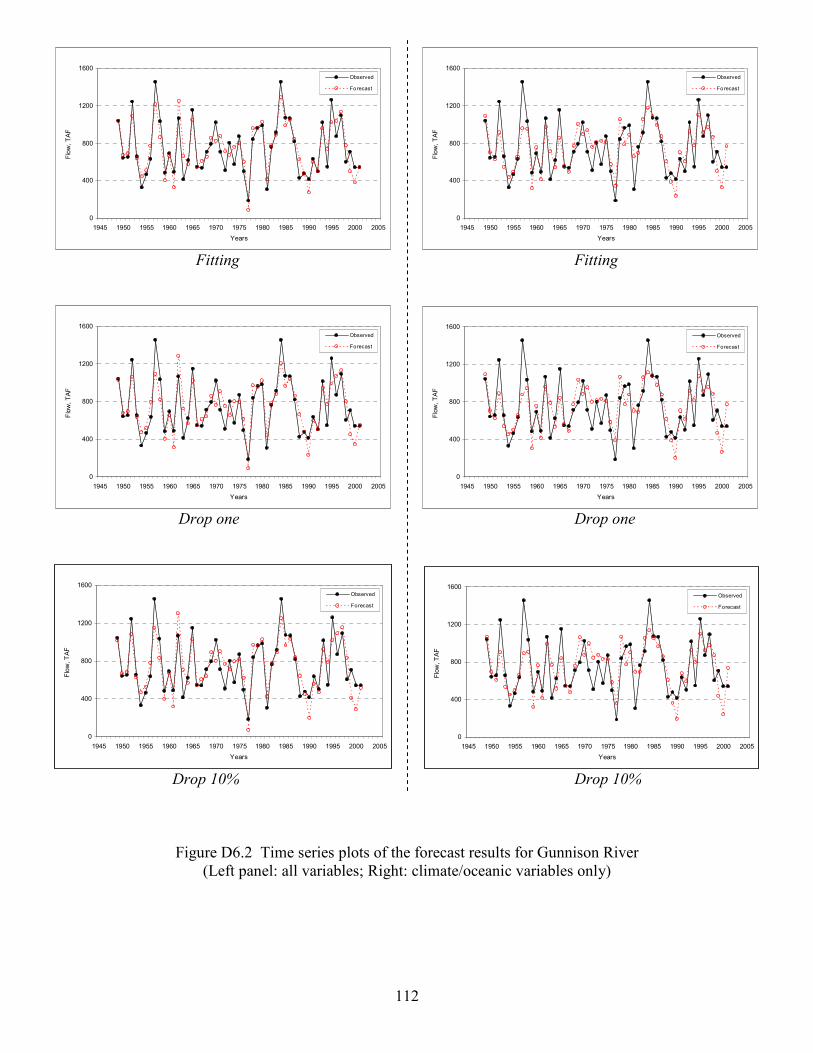
112

0

400

800

1200

1600

1945 1950 1955 1960 1965 1970 1975 1980 1985 1990 1995 2000 2005

Years

Flo

w,

TA

F

Observed

Forecast

0

400

800

1200

1600

1945 1950 1955 1960 1965 1970 1975 1980 1985 1990 1995 2000 2005

Years

Flo

w,

TA

F

Observed

Forecast

Fitting Fitting

0

400

800

1200

1600

1945 1950 1955 1960 1965 1970 1975 1980 1985 1990 1995 2000 2005

Years

Flo

w, T

AF

Observed

Forecast

0

400

800

1200

1600

1945 1950 1955 1960 1965 1970 1975 1980 1985 1990 1995 2000 2005

Years

Flo

w, T

AF

Observed

Forecast

Drop one Drop one

0

400

800

1200

1600

1945 1950 1955 1960 1965 1970 1975 1980 1985 1990 1995 2000 2005

Years

Flo

w, T

AF

Observed

Forecast

0

400

800

1200

1600

1945 1950 1955 1960 1965 1970 1975 1980 1985 1990 1995 2000 2005

Years

Flo

w, T

AF

Observed

Forecast

Drop 10% Drop 10%

Figure D6.2 Time series plots of the forecast results for Gunnison River

(Left panel: all variables; Right: climate/oceanic variables only)

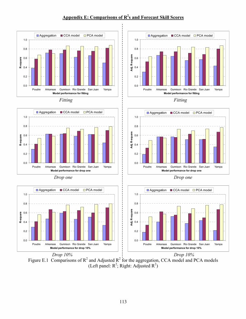
113

Appendix E: Comparisons of R2s and Forecast Skill Scores

0.0

0.2

0.4

0.6

0.8

1.0

Poudre Arkansas Gunnison Rio Grande San Juan Yampa

Model performance for fitting

R-square

Aggregation CCA model PCA model

0.0

0.2

0.4

0.6

0.8

1.0

Poudre Arkansas Gunnison Rio Grande San Juan Yampa

Model performance for fitting

Adj. R-square

Aggregation CCA model PCA model

Fitting Fitting

0.0

0.2

0.4

0.6

0.8

1.0

Poudre Arkansas Gunnison Rio Grande San Juan Yampa

Model performance for drop one

R-square

Aggregation CCA model PCA model

0.0

0.2

0.4

0.6

0.8

1.0

Poudre Arkansas Gunnison Rio Grande San Juan Yampa

Model performance for drop one

Adj. R-square

Aggregation CCA model PCA model

Drop one Drop one

0.0

0.2

0.4

0.6

0.8

1.0

Poudre Arkansas Gunnison Rio Grande San Juan Yampa

Model performance for drop 10%

R-square

Aggregation CCA model PCA model

0.0

0.2

0.4

0.6

0.8

1.0

Poudre Arkansas Gunnison Rio Grande San Juan Yampa

Model performance for drop 10%

Adj. R-square

Aggregation CCA model PCA model

Drop 10% Drop 10%

Figure E.1 Comparisons of R2 and Adjusted R

2 for the aggregation, CCA model and PCA models

(Left panel: R2; Right: Adjusted R

2)

114

0.0

0.2

0.4

0.6

0.8

1.0

Poudre Arkansas Gunnison Rio Grande San Juan Yampa

Forecast skills for fitting

Accuracy

Aggregation CCA model PCA model

0.0

0.2

0.4

0.6

0.8

1.0

Poudre Arkansas Gunnison Rio Grande San Juan Yampa

Forecast skills for fitting

HSS

Aggregation CCA model PCA model

Fitting Fitting

0.0

0.2

0.4

0.6

0.8

1.0

Poudre Arkansas Gunnison Rio Grande San Juan Yampa

Forecast skills for drop one

Accuracy

Aggregation CCA model PCA model

0.0

0.2

0.4

0.6

0.8

1.0

Poudre Arkansas Gunnison Rio Grande San Juan Yampa

Forecast skills for drop one

HSS

Aggregation CCA model PCA model

Drop one Drop one

0.0

0.2

0.4

0.6

0.8

1.0

Poudre Arkansas Gunnison Rio Grande San Juan Yampa

Forecast skills for drop 10%

Accuracy

Aggregation CCA model PCA model

0.0

0.2

0.4

0.6

0.8

1.0

Poudre Arkansas Gunnison Rio Grande San Juan Yampa

Forecast skills for drop 10%

HSS

Aggregation CCA model PCA model

Drop 10% Drop 10%

Figure E.2 Comparisons of forecast skill scores for the aggregation, CCA model and PCA models

(Left panel: Accuracy; Right: HSS)

115

0.0

0.2

0.4

0.6

0.8

1.0

April - July April May June July

Poudre River

R2 and adj. R2

R2 adj. R2

0.0

0.2

0.4

0.6

0.8

1.0

April - July April May June July

Arkansas River

R2 and adj. R2

R2 adj. R2

0.0

0.2

0.4

0.6

0.8

1.0

April - July April May June July

Gunnison River

R2 and adj. R2

R2 adj. R2

0.0

0.2

0.4

0.6

0.8

1.0

April - July April May June July

Rio Grande

R2 and adj. R2

R2 adj. R2

0.0

0.2

0.4

0.6

0.8

1.0

April - July April May June July

San Juan River

R2 and adj. R2

R2 adj. R2

0.0

0.2

0.4

0.6

0.8

1.0

April - July April May June July

Yampa River

R2 and adj. R2

R2 adj. R2

Figure E.3 Comparisons of R2 and Adjusted R

2 for the PCA model and the temporal disaggregation (fitting)

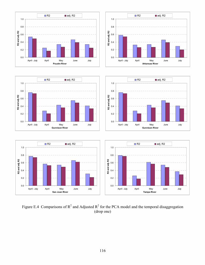
116

0.0

0.2

0.4

0.6

0.8

1.0

April - July April May June July

Poudre River

R2 and adj. R2

R2 adj. R2

0.0

0.2

0.4

0.6

0.8

1.0

April - July April May June July

Arkansas River

R2 and adj. R2

R2 adj. R2

0.0

0.2

0.4

0.6

0.8

1.0

April - July April May June July

Gunnison River

R2 and adj. R2

R2 adj. R2

0.0

0.2

0.4

0.6

0.8

1.0

April - July April May June July

Gunnison River

R2 and adj. R2

R2 adj. R2

0.0

0.2

0.4

0.6

0.8

1.0

April - July April May June July

San Juan River

R2 and adj. R2

R2 adj. R2

0.0

0.2

0.4

0.6

0.8

1.0

April - July April May June July

Yampa River

R2 and adj. R2

R2 adj. R2

Figure E.4 Comparisons of R2 and Adjusted R

2 for the PCA model and the temporal disaggregation

(drop one)

117

0.0

0.2

0.4

0.6

0.8

1.0

April - July April May June July

Poudre River

R2 and adj. R2

R2 adj. R2

0.0

0.2

0.4

0.6

0.8

1.0

April - July April May June July

Arkansas River

R2 and adj. R2

R2 adj. R2

0.0

0.2

0.4

0.6

0.8

1.0

April - July April May June July

Gunnison River

R2 and adj. R2

R2 adj. R2

0.0

0.2

0.4

0.6

0.8

1.0

April - July April May June July

Rio Grande

R2 and adj. R2

R2 adj. R2

0.0

0.2

0.4

0.6

0.8

1.0

April - July April May June July

San Juan River

R2 and adj. R2

R2 adj. R2

0.0

0.2

0.4

0.6

0.8

1.0

April - July April May June July

Yampa River

R2 and adj. R2

R2 adj. R2

Figure E.5 Comparisons of R2 and Adjusted R

2 for the PCA model and the temporal disaggregation

(drop 10%)

118

0.0

0.2

0.4

0.6

0.8

1.0

April - July April May June July

Poudre River

Accuracy and HSS

Accuracy HSS

0.0

0.2

0.4

0.6

0.8

1.0

April - July April May June July

Arkansas River

Accuracy and HSS

Accuracy HSS

0.0

0.2

0.4

0.6

0.8

1.0

April - July April May June July

Gunnison River

Accuracy and HSS

Accuracy HSS

0.0

0.2

0.4

0.6

0.8

1.0

April - July April May June July

Rio Grande

Accuracy and HSS

Accuracy HSS

0.0

0.2

0.4

0.6

0.8

1.0

April - July April May June July

San Juan River

Accuracy and HSS

Accuracy HSS

0.0

0.2

0.4

0.6

0.8

1.0

April - July April May June July

Yampa River

Accuracy and HSS

Accuracy HSS

Figure E.6 Comparisons of forecast skills for the PCA model and the temporal disaggregation (fitting)

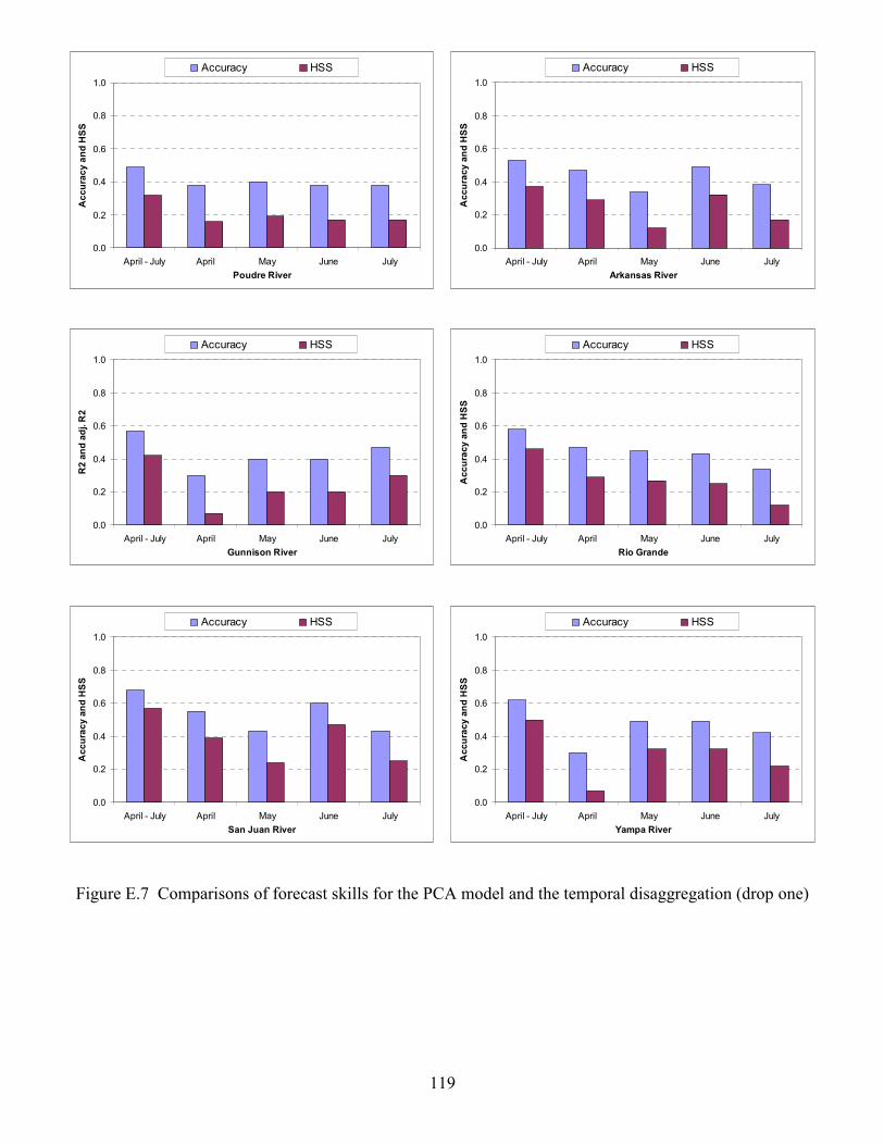
119

0.0

0.2

0.4

0.6

0.8

1.0

April - July April May June July

Poudre River

Accuracy and HSS

Accuracy HSS

0.0

0.2

0.4

0.6

0.8

1.0

April - July April May June July

Arkansas River

Accuracy and HSS

Accuracy HSS

0.0

0.2

0.4

0.6

0.8

1.0

April - July April May June July

Gunnison River

R2 and adj. R2

Accuracy HSS

0.0

0.2

0.4

0.6

0.8

1.0

April - July April May June July

Rio Grande

Accuracy and HSS

Accuracy HSS

0.0

0.2

0.4

0.6

0.8

1.0

April - July April May June July

San Juan River

Accuracy and HSS

Accuracy HSS

0.0

0.2

0.4

0.6

0.8

1.0

April - July April May June July

Yampa River

Accuracy and HSS

Accuracy HSS

Figure E.7 Comparisons of forecast skills for the PCA model and the temporal disaggregation (drop one)

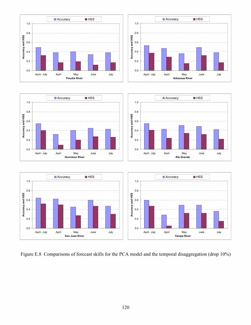
120

0.0

0.2

0.4

0.6

0.8

1.0

April - July April May June July

Poudre River

Accuracy and HSS

Accuracy HSS

0.0

0.2

0.4

0.6

0.8

1.0

April - July April May June July

Arkansas River

Accuracy and HSS

Accuracy HSS

0.0

0.2

0.4

0.6

0.8

1.0

April - July April May June July

Gunnison River

Accuracy and HSS

Accuracy HSS

0.0

0.2

0.4

0.6

0.8

1.0

April - July April May June July

Rio Grande

Accuracy and HSS

Accuracy HSS

0.0

0.2

0.4

0.6

0.8

1.0

April - July April May June July

San Juan River

Accuracy and HSS

Accuracy HSS

0.0

0.2

0.4

0.6

0.8

1.0

April - July April May June July

Yampa River

Accuracy and HSS

Accuracy HSS

Figure E.8 Comparisons of forecast skills for the PCA model and the temporal disaggregation (drop 10%)