65

5. DUAL LP, SOLUTION INTERPRETATION, ANDPOST-OPTIMALITY

5.1 DUALITY

Associated with every linear programming problem (the primal) is another linear programmingproblem called its dual. If the primal involves n variables and m constraints, the dual involves nconstraints and m variables. The solution to either is sufficient for readily obtaining the solutionto the other. In fact, it is immaterial which is designated as the primal since the dual of a dual isthe primal.

Suppose that the primal problem is:

Max Z = C1 X1 + C2 X2 + ... + Cn Xn ...[5.1]

s.t.: A11 X1 + A12 X2 + ... + A1n Xn ≤ B1 ...[5.2]

A21 X1 + A22 X2 + ... + A2n Xn ≤ B2

...

Am1 X1 + Am2 X2 + ... + Amn Xn ≤ Bm

Xj ≥ 0 (for j = 1, 2, ..., n) ...[5.3]

or

Max Z = CTX ...[5.4]

s.t.: AX ≤ B ...[5.5]

If the above (Expressions [5.1] through [5.5]) is the primal LP problem, the dual problem is:

Min ˜ Z = B1 Y1 + B2 Y2 + ... + Bm Ym ...[5.6]

s.t.: A11 Y1 + A21 Y2 + ... + Am1 Ym ≥ C1 ...[5.7]

A12 Y1 + A22 Y2 + ... + Am2 Ym ≥ C2 ...[5.8]

...

A1n Y1 + A2n Y2 + ... + Amn Ym ≥ Cn ...[5.9]

66

Yi ≥ 0 (for all i = 1, 2, ..., m) ...[5.10]

or

Min ˜ Z = BTY ...[5.11]

s.t.: ATY ≥ C ...[5.12]

The variables Yi are called the “dual variables”. One dual variable will be associated with eachconstraint in the primal problem. Note that equality constraints are either replaced by two ine-qualities or, if left as an equality, then the associated dual variable is unrestricted in sign.

5.2 AN EXAMPLE OF THE PRIMAL-DUAL RELATIONSHIP

Consider the following primal problem and its corresponding dual:

Primal Problem:

Min Zx = 10 X1 + 4 X2 ...[5.13]

Dual Variables

s.t.: X1 ≥ 4 Y1 ...[5.14]

X2 ≥ 6 Y2 ...[5.15]

X1 + 2 X2 ≥ 20 Y3 ...[5.16]

2 X1 + X2 ≥ 17 Y4 ...[5.17]

Dual Problem:

Max Zy = 4 Y1 + 6 Y2 + 20 Y3 + 17 Y4 ...[5.18]

s.t.: Y1 + Y3 + 2 Y4 ≤ 10 ...[5.19]

Y2 + 2 Y3 + Y4 ≤ 4 ...[5.20]

The solutions for these two linear optimization problems are:

67

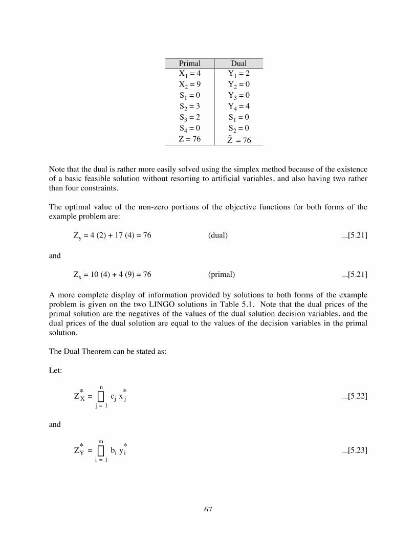
Primal DualX1 = 4X2 = 9S1 = 0S2 = 3S3 = 2S4 = 0Z = 76

Y1 = 2Y2 = 0Y3 = 0Y4 = 4S1 = 0S2 = 0˜ Z = 76

Note that the dual is rather more easily solved using the simplex method because of the existenceof a basic feasible solution without resorting to artificial variables, and also having two ratherthan four constraints.

The optimal value of the non-zero portions of the objective functions for both forms of theexample problem are:

Zy = 4 (2) + 17 (4) = 76 (dual) ...[5.21]

and

Zx = 10 (4) + 4 (9) = 76 (primal) ...[5.21]

A more complete display of information provided by solutions to both forms of the exampleproblem is given on the two LINGO solutions in Table 5.1. Note that the dual prices of theprimal solution are the negatives of the values of the dual solution decision variables, and thedual prices of the dual solution are equal to the values of the decision variables in the primalsolution.

The Dual Theorem can be stated as:

Let:

Z X* =

j = 1

n

 cj x j* ...[5.22]

and

ZY* =

i = 1

m

 bi yi* ...[5.23]

68

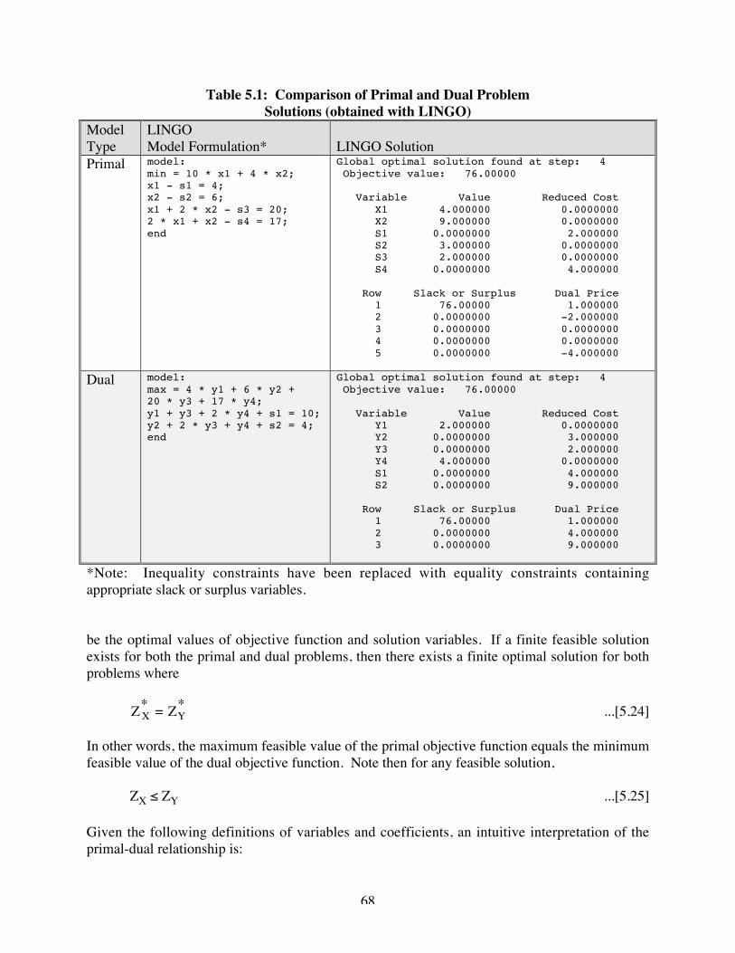
Table 5.1: Comparison of Primal and Dual ProblemSolutions (obtained with LINGO)

ModelType

LINGOModel Formulation* LINGO Solution

Primal model:min = 10 * x1 + 4 * x2;x1 - s1 = 4;x2 - s2 = 6;x1 + 2 * x2 - s3 = 20;2 * x1 + x2 - s4 = 17;end

Global optimal solution found at step: 4 Objective value: 76.00000

Variable Value Reduced Cost X1 4.000000 0.0000000 X2 9.000000 0.0000000 S1 0.0000000 2.000000 S2 3.000000 0.0000000 S3 2.000000 0.0000000 S4 0.0000000 4.000000

Row Slack or Surplus Dual Price 1 76.00000 1.000000 2 0.0000000 -2.000000 3 0.0000000 0.0000000 4 0.0000000 0.0000000 5 0.0000000 -4.000000

Dual model:max = 4 * y1 + 6 * y2 +20 * y3 + 17 * y4;y1 + y3 + 2 * y4 + s1 = 10;y2 + 2 * y3 + y4 + s2 = 4;end

Global optimal solution found at step: 4 Objective value: 76.00000

Variable Value Reduced Cost Y1 2.000000 0.0000000 Y2 0.0000000 3.000000 Y3 0.0000000 2.000000 Y4 4.000000 0.0000000 S1 0.0000000 4.000000 S2 0.0000000 9.000000

Row Slack or Surplus Dual Price 1 76.00000 1.000000 2 0.0000000 4.000000 3 0.0000000 9.000000

*Note: Inequality constraints have been replaced with equality constraints containingappropriate slack or surplus variables.

be the optimal values of objective function and solution variables. If a finite feasible solutionexists for both the primal and dual problems, then there exists a finite optimal solution for bothproblems where

Z X* = ZY

* ...[5.24]

In other words, the maximum feasible value of the primal objective function equals the minimumfeasible value of the dual objective function. Note then for any feasible solution,

ZX ≤ ZY ...[5.25]

Given the following definitions of variables and coefficients, an intuitive interpretation of theprimal-dual relationship is:

69

Primal Dual

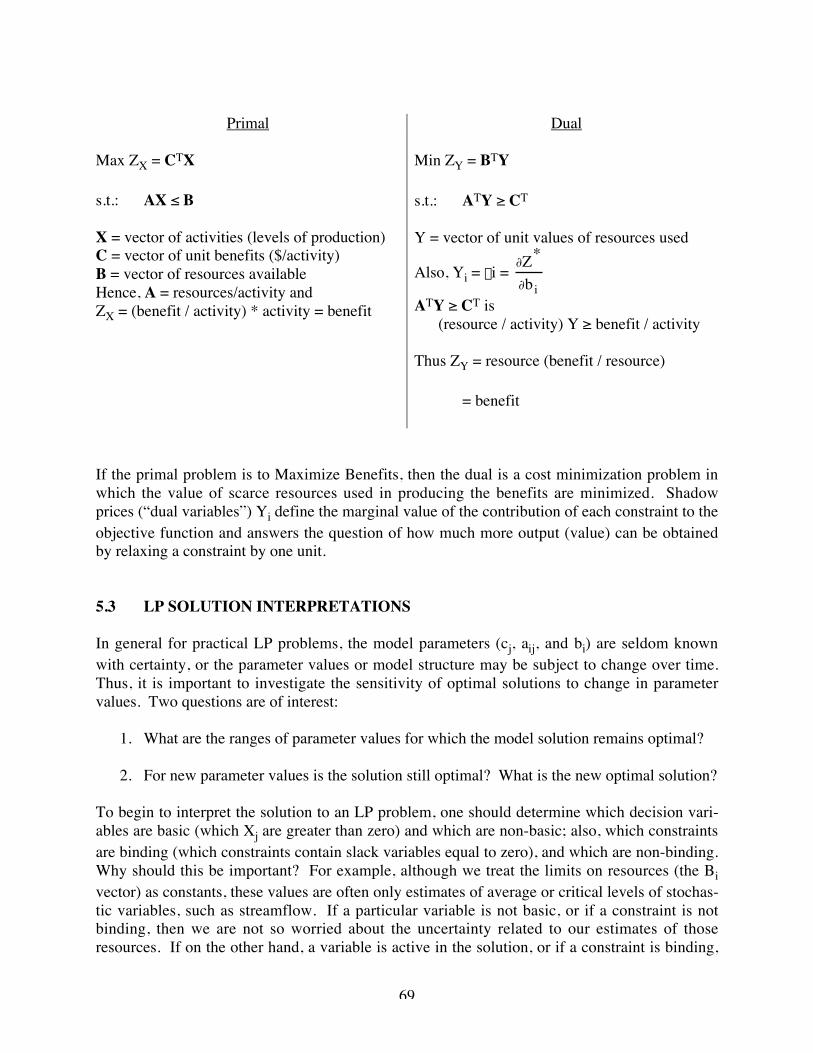
Max ZX = CTX

s.t.: AX ≤ B

X = vector of activities (levels of production)C = vector of unit benefits ($/activity)B = vector of resources availableHence, A = resources/activity andZX = (benefit / activity) * activity = benefit

Min ZY = BTY

s.t.: ATY ≥ CT

Y = vector of unit values of resources used

Also, Yi = li = ∂Z*

∂biATY ≥ CT is

(resource / activity) Y ≥ benefit / activity

Thus ZY = resource (benefit / resource)

= benefit

If the primal problem is to Maximize Benefits, then the dual is a cost minimization problem inwhich the value of scarce resources used in producing the benefits are minimized. Shadowprices (“dual variables”) Yi define the marginal value of the contribution of each constraint to theobjective function and answers the question of how much more output (value) can be obtainedby relaxing a constraint by one unit.

5.3 LP SOLUTION INTERPRETATIONS

In general for practical LP problems, the model parameters (cj, aij, and bi) are seldom knownwith certainty, or the parameter values or model structure may be subject to change over time.Thus, it is important to investigate the sensitivity of optimal solutions to change in parametervalues. Two questions are of interest:

1. What are the ranges of parameter values for which the model solution remains optimal?

2. For new parameter values is the solution still optimal? What is the new optimal solution?

To begin to interpret the solution to an LP problem, one should determine which decision vari-ables are basic (which Xj are greater than zero) and which are non-basic; also, which constraintsare binding (which constraints contain slack variables equal to zero), and which are non-binding.Why should this be important? For example, although we treat the limits on resources (the Bivector) as constants, these values are often only estimates of average or critical levels of stochas-tic variables, such as streamflow. If a particular variable is not basic, or if a constraint is notbinding, then we are not so worried about the uncertainty related to our estimates of thoseresources. If on the other hand, a variable is active in the solution, or if a constraint is binding,

70

then we would like to know how important are errors in our estimates of those resources or ofunit costs or benefits from those variables. Various types of sensitivity analysis can answer suchquestions.

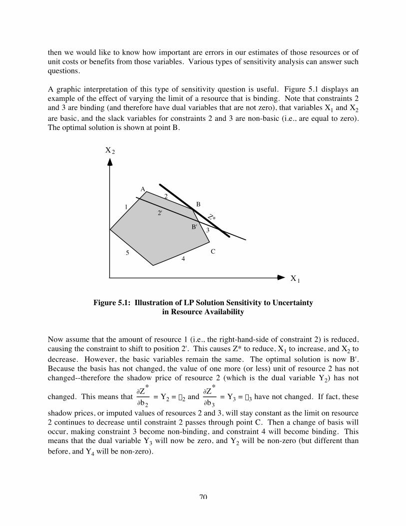
A graphic interpretation of this type of sensitivity question is useful. Figure 5.1 displays anexample of the effect of varying the limit of a resource that is binding. Note that constraints 2and 3 are binding (and therefore have dual variables that are not zero), that variables X1 and X2are basic, and the slack variables for constraints 2 and 3 are non-basic (i.e., are equal to zero).The optimal solution is shown at point B.

X 2

X 1

12

3

45

A

B

C

Z*B'

2'

Figure 5.1: Illustration of LP Solution Sensitivity to Uncertaintyin Resource Availability

Now assume that the amount of resource 1 (i.e., the right-hand-side of constraint 2) is reduced,causing the constraint to shift to position 2'. This causes Z* to reduce, X1 to increase, and X2 todecrease. However, the basic variables remain the same. The optimal solution is now B'.Because the basis has not changed, the value of one more (or less) unit of resource 2 has notchanged--therefore the shadow price of resource 2 (which is the dual variable Y2) has not

changed. This means that ∂Z*

∂b2 = Y2 = l2 and ∂Z*

∂b3 = Y3 = l3 have not changed. If fact, these

shadow prices, or imputed values of resources 2 and 3, will stay constant as the limit on resource2 continues to decrease until constraint 2 passes through point C. Then a change of basis willoccur, making constraint 3 become non-binding, and constraint 4 will become binding. Thismeans that the dual variable Y3 will now be zero, and Y2 will be non-zero (but different thanbefore, and Y4 will be non-zero).

71

Some LP algorithms have a utility called RANGE that produces information on the range overwhich and right-hand-side (RHS) can vary before the shadow prices (the dual variables) change.The LINGO solutions give the value of the shadow prices in the column of the ROWS sectionlabeled DUAL PRICE. We now have several names for the same parameter, as follows:

Yi = l i = shadow price = imputed value of resource = dual price = dual variable = ∂Z*

∂bi

5.4 SENSITIVITY ANALYSIS OF OBJECTIVE COEFFICIENTS (Cj)

Another type of sensitivity analysis considers the effect of varying the values of the cost, or Cj,coefficients (the value or cost of one unit of Xj). Imagine what would happen if the values ofeither C1 or C2 or both were to change. This would cause the slope of the objective function, Z,to increase or decrease. This would change the value of Z*, but not the optimal level of X1 or X2(and therefore there would not be a basis change) unless the change causes the slope of Z toincrease enough to equal or exceed the slope of constraint 3 (refer to Figure 5.1). At this point achange of basic variables would occur, and X1

* and X2* would change.

The LINGO solution file has a column in the Variables section labeled REDUCED COST. Thiscolumn gives the change in Z* per unit Xj if a non-basic Xj were to enter the basis. That is,

REDUCED COST = ∂Z*

∂xj...[5.26]

for non-basic Xj.

5.5 PARAMETRIC PROGRAMMING

The following distinction is made between sensitivity analysis and parametric programming:

1. Sensitivity analysis--examination of discrete parameter changes

2. Parametric programming--analysis of changes in optimal solutions for continuous or sys-tematic parameter changes of one or several parameters simultaneously.

The general types of parameter and model structure changes to be examined in LP problems are:

1. Objective function coefficients, Cj

2. Resource limits or RHS values, Bi

72

3. Changes in technical (constraint) coefficients, Aij

4. Effect of an additional constraint

5. Effect of additional variables

5.5.1 Changes in Objective Function Coefficients, Cj

To evaluate changes in objective function coefficients, the original objective function

Z = j = 1

n

 Cj Xj ...[5.27]

is rewritten as:

Z = j = 1

n

 (Cj + qj) Xj ...[5.28]

where the qjs are relative rates of change for the Cjs. Note, for qj = 0, we have the original LPproblem. qj varies from zero to some specified positive number, V, such that 0 ≤ qj ≤ V. Thegoal is to find an optimal solution to the modified LP problem (subject to the original con-straints) as a function of q. The parametric analysis must determine when and how the optimalsolution changes, and to what, over the range of q.

5.5.2 Changes in Resource Limits, Bi

The effects of changes in resource limits as expressed in an LP model can be evaluated in afashion similar to the above analysis of the Cjs. For this, the original constraint

j = 1

n

 Aij Xj ≤ Bi (i = 1, 2, ..., m) ...[5.29]

is rewritten as:

j = 1

n

 Aij Xj ≤ Bi + ai (i = 1, 2, ..., m) ...[5.30]

and the LP problem is then solved as the value of ai is varied over a range. The goal is to iden-tify changes in optimal solutions as a function of ai.

73

5.5.3 Strategy of Post-Optimality Analysis

Clearly, adjusting the model, resolving, and comparing could get answers to questions posed.Research devoted to the subject has developed more efficient procedures by working from thepresent optimal solution. Procedures are usually available as part of standard computer LP pack-ages.

74

5.6 PROBLEMS

1. Solve (using LINGO) both the primal and the dual of the following problem and comparethe solutions:

Max Z = 2 A + 3 B + C

s.t.: A + 5 B ≤ 15

A + B + C ≥ 6

A ≥ B + C

a. What are the dual prices of the primal? How do they compare to the decision vari-ables of the dual?

b. What are the dual prices of the dual, and how do they compare with the decision vari-ables of the primal?

2. Repeat Problem 1, above, with the inequality in the last constraint changed to an equality.

Note: The following procedure will help avoid errors in the homework, and is highly rec-ommended:

a. Before writing the dual, always convert the constraints into the following form:

• for maximization problems, make all constraints take the form g(x ) ≤ b bychanging signs if necessary

• for minimization problems, make all constraints take the form g(x) ≥ b, again bychanging signs if necessary

b. For a strict equality constraint, specify that the corresponding dual variable is unre-stricted in sign. However, since the simplex method does not in general allow nega-tive decision variables, if you were doing a simplex solution by hand you could usethe following transform:

Y1 = Ya - Yb

Then, Ya and Yb would be set in the optimal simplex solution to be nonnegative.

For a manual derivation of the dual, replace the single primal constraint with twoconstraints that are it’s equivalent. For example, if the primal problem includes:

75

Max Z

s.t.: 2 X1 + X2 = 5

replace the above equality constraint with the following two constraints:

2 X1 + X2 ≤ 5

2 X1 + X2 ≥ 5

Then convert the second inequality constraint into:

-2 X1 - X2 ≤ -5

before writing the dual.

76

(this page is left intentionally blank)