Embed Size (px)
Citation preview
8/6/2019 Long Term and Shrt Run relationship between Macroeconomic variables and stock market in India
http://slidepdf.com/reader/full/long-term-and-shrt-run-relationship-between-macroeconomic-variables-and-stock 1/48
1
University of Newcastle Upon Tyne
Business School
MSc. International Economics and Finance
IS THERE A LONG RUN EQUILIBRIUM AND SHORT RUN DYNAMIC RELATIONSHIP BETWEEN
MACROECONOMIC VARIABLES AND STOCK PRICES IN INDIA?
Supervisor: Dr. Simon Vicary
June 2010

8/6/2019 Long Term and Shrt Run relationship between Macroeconomic variables and stock market in India
http://slidepdf.com/reader/full/long-term-and-shrt-run-relationship-between-macroeconomic-variables-and-stock 2/48
2
Dedication
This dissertation is dedicated to my parents and sisters.

8/6/2019 Long Term and Shrt Run relationship between Macroeconomic variables and stock market in India
http://slidepdf.com/reader/full/long-term-and-shrt-run-relationship-between-macroeconomic-variables-and-stock 3/48
3
Acknowledgements
I would like to express my gratitude to my supervisor and personal tutor, Dr. Simon Vicary,
for his guidance and support throughout the dissertation work.
I would like to thank all my professors for their support all the year which was a great help
for me.
I would like to thank my parents for giving me motivation and determination to complete
this dissertation. I would also like to thank my friends for helping me out in small issues that
made this dissertation look better.
8/6/2019 Long Term and Shrt Run relationship between Macroeconomic variables and stock market in India
http://slidepdf.com/reader/full/long-term-and-shrt-run-relationship-between-macroeconomic-variables-and-stock 4/48
4
Abstract
Understanding the reasons for the changes in stock prices has always been
topic of interest among analysts and investors. This study aims at finding the
effects of changes in macroeconomic variables on stock prices in long run and
short run for Indian economy using Vector auto regression, impulse response,
forecast error variance decomposition and Granger Causality. Results show
that stock prices are not related to macroeconomic variable in long run or
short run. Only exception is Exchange Rate which affects stock prices in short
run. This study shows that stock prices are not much dependent on domestic
factors.
8/6/2019 Long Term and Shrt Run relationship between Macroeconomic variables and stock market in India
http://slidepdf.com/reader/full/long-term-and-shrt-run-relationship-between-macroeconomic-variables-and-stock 5/48
5
Table of Contents
Abstract.........................................................................................................................4
Table of Contents...........................................................................................................5
List of Figures.................................................................................................................6
List of Tables...................................................................................................................7
1.0 Introduction.....................................................................................................9
1.1 Development of Indian Economy....................................................9
2.0 Literature Review............................................................................................12
2.1 Chronological Review of Literature................................................13
3.0 Theoretical Framework...................................................................................19
(3.1) Inflation..........................................................................................19
(3.2) Exchange Rate................................................................................20
(3.3) Money Supply.................................................................................20
(3.4) Interest Rate...................................................................................21
(3.5) Industrial Production......................................................................21
4.0 Empirical Framework......................................................................................21
(4.1) Stationary and Non Stationary Data...............................................21
(4.2) Augmented Dickey Fuller................................................................22
(4.3) Engle Granger Cointegration Test...................................................23
(4.4) Granger Causality...........................................................................23
(4.5) Vector Auto Regression (VAR)........................................................24
(4.5.1) Variance Decomposition............................................26
8/6/2019 Long Term and Shrt Run relationship between Macroeconomic variables and stock market in India
http://slidepdf.com/reader/full/long-term-and-shrt-run-relationship-between-macroeconomic-variables-and-stock 6/48
6
(4.5.2) Impulse Response......................................................26
5.0 Tests and Results..............................................................................................26
6.0 Conclusion.........................................................................................................35
7.0 References........................................................................................................37
8.0 Appendix...........................................................................................................39
8/6/2019 Long Term and Shrt Run relationship between Macroeconomic variables and stock market in India
http://slidepdf.com/reader/full/long-term-and-shrt-run-relationship-between-macroeconomic-variables-and-stock 7/48
7
List of Figures
Figure 1............................................................................................................................10
Figure 2.............................................................................................................................30
Figure 3.............................................................................................................................30
Figure 4.............................................................................................................................30
Figure 5..............................................................................................................................30
Figure 6..............................................................................................................................30
8/6/2019 Long Term and Shrt Run relationship between Macroeconomic variables and stock market in India
http://slidepdf.com/reader/full/long-term-and-shrt-run-relationship-between-macroeconomic-variables-and-stock 8/48
8
List of Tables
Table 1.........................................................................................................................27
Table 2.........................................................................................................................27
Table 3..........................................................................................................................28
Table 4..........................................................................................................................28
Table 5..........................................................................................................................31
Table 6...........................................................................................................................31
Table 7...........................................................................................................................32
Table 8...........................................................................................................................32
Table 9...........................................................................................................................33
Table 10.........................................................................................................................34
Table 11.........................................................................................................................34
Table 12.........................................................................................................................39
Table 13.........................................................................................................................40
Table 14..........................................................................................................................42
Table 15..........................................................................................................................43
Table 16..........................................................................................................................45
Table 17..........................................................................................................................46
8/6/2019 Long Term and Shrt Run relationship between Macroeconomic variables and stock market in India
http://slidepdf.com/reader/full/long-term-and-shrt-run-relationship-between-macroeconomic-variables-and-stock 9/48
9
(1) Introduction:
This dissertation is an attempt to study the long run equilibrium and short run dynamic
relationship of Indian Stock Market with its Macroeconomic variables during 1991 to 2009.
Reason for choosing this study was the fact that there had been very less research work
done on relationship between stock prices and macroeconomic variables for developing
countries, especially India, whereas one can find lot of work in this field for developed
economies like US, UK, Japan and other European economies. Most of the studies on this
topic, in relation to Indian economy, have been very limited in terms of number of variables
used in research. Some studies have been done on Indian economy but those were
concentrated on developing nations as a whole rather than looking specifically at India. I
could not find any research paper using five macroeconomic variables to find the
relationship between macroeconomic variables and stock prices in India. In this topic I am
trying to find whether a dynamic relationship between Indian stock market Growth and
macroeconomic variables exists in long run and short run. In emerging economies like India,
often the company information is late and of low standards which makes it difficult to
correctly evaluate the true value of company shares (Bekaert and Harvey 1998). Few
questions that need to be answered through this dissertation are
Is there long run equilibrium between Indian Stock Prices and its macroeconomic
variables?
Is there a short run causal relationship between variables?
How much one variable can be explained by innovation in other variable?
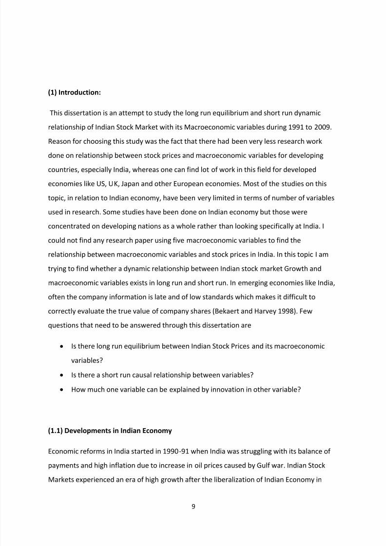
(1.1) Developments in Indian Economy
Economic reforms in India started in 1990-91 when India was struggling with its balance of
payments and high inflation due to increase in oil prices caused by Gulf war. Indian Stock
Markets experienced an era of high growth after the liberalization of Indian Economy in
8/6/2019 Long Term and Shrt Run relationship between Macroeconomic variables and stock market in India
http://slidepdf.com/reader/full/long-term-and-shrt-run-relationship-between-macroeconomic-variables-and-stock 10/48
10
1991. Indian economy was on the brink of bankruptcy as foreign reserves were almost
extinct in 1991 with inflation as high as 11% and economy was about to collapse. Then
finance minister and current Prime Minister of India Mr. Manmohan Singh took first step
towards liberalization by privatizing sectors like Telecom, Aviation, Banks etc. and openingup the gates for FDIs and FIIs in India and hence calling an end to high tax regime in India.
With more flow of foreign capital, the Indian stock markets saw its capitalization going up
exponentially. From the period between 1990 and 2010, Indian economy has grown at more
than 6% annually. Economic reforms helped boost sectors like Information Technology,
Pharmaceuticals, Telecom, Aviation, banking, textile and Real Estate which lead to more
private players playing important role in the economy. In 2009, seven Indian firms were
listed among the top 15 technology outsourcing companies in the world.
While the credit
rating of India was hit by its nuclear tests in 1998, it has been raised to investment level in
2007 by S&P and Moody's.
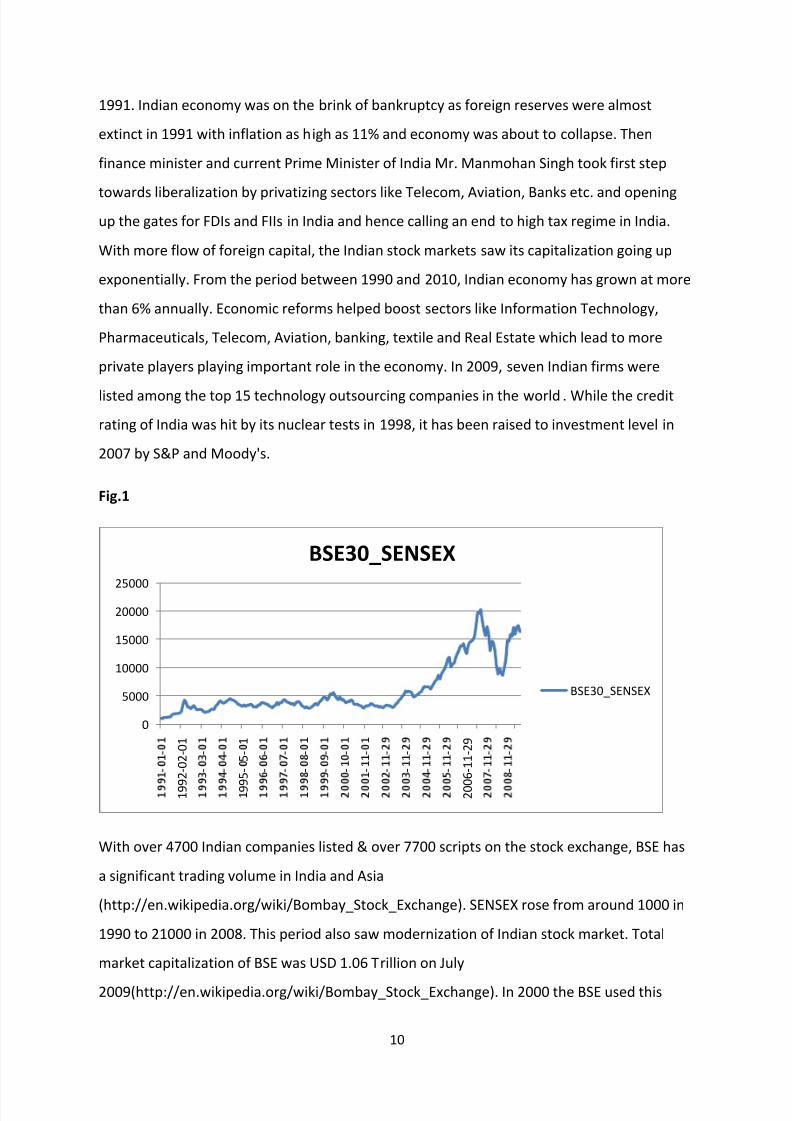
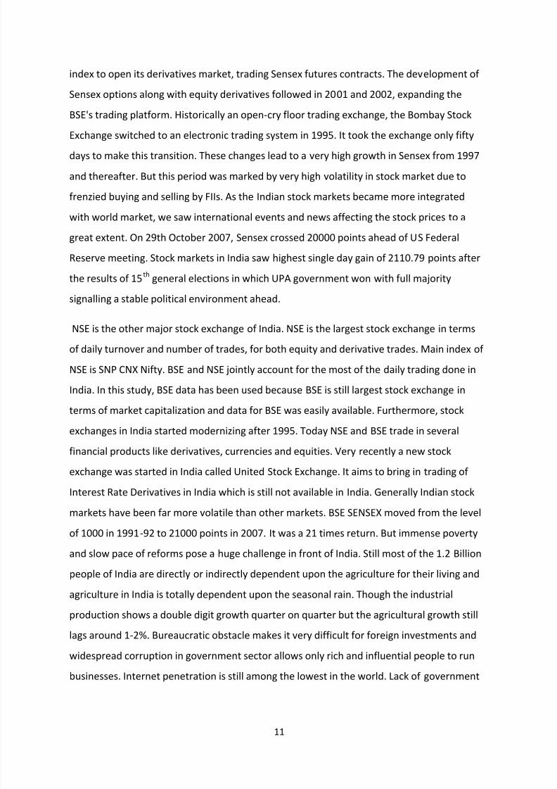
Fig.1
With over 4700 Indian companies listed & over 7700 scripts on the stock exchange, BSE has
a significant trading volume in India and Asia
(http://en.wikipedia.org/wiki/Bombay_Stock_Exchange). SENSEX rose from around 1000 in
1990 to 21000 in 2008. This period also saw modernization of Indian stock market. Total
market capitalization of BSE was USD 1.06 Trillion on July
2009(http://en.wikipedia.org/wiki/Bombay_Stock_Exchange). In 2000 the BSE used this
0
5000
10000
15000
20000
25000
-
-
1 9 9 2 - 0 2 - 0 1
-
-
-
-
9 9 5 -
5 -
1
-
-
-
-
-
-
-
-
-
-
-
-
-
-
-
-
-
-
-
-
2 0 0 6 - 1 1 - 2 9
-
-
-
-
BSE30_SENSEX
BSE30_SENSEX
8/6/2019 Long Term and Shrt Run relationship between Macroeconomic variables and stock market in India
http://slidepdf.com/reader/full/long-term-and-shrt-run-relationship-between-macroeconomic-variables-and-stock 11/48
11
index to open its derivatives market, trading Sensex futures contracts. The development of
Sensex options along with equity derivatives followed in 2001 and 2002, expanding the
BSE's trading platform. Historically an open-cry floor trading exchange, the Bombay Stock
Exchange switched to an electronic trading system in 1995. It took the exchange only fiftydays to make this transition. These changes lead to a very high growth in Sensex from 1997
and thereafter. But this period was marked by very high volatility in stock market due to
frenzied buying and selling by FIIs. As the Indian stock markets became more integrated
with world market, we saw international events and news affecting the stock prices to a
great extent. On 29th October 2007, Sensex crossed 20000 points ahead of US Federal
Reserve meeting. Stock markets in India saw highest single day gain of 2110.79 points after
the results of 15th general elections in which UPA government won with full majority
signalling a stable political environment ahead.
NSE is the other major stock exchange of India. NSE is the largest stock exchange in terms
of daily turnover and number of trades, for both equity and derivative trades. Main index of
NSE is SNP CNX Nifty. BSE and NSE jointly account for the most of the daily trading done in
India. In this study, BSE data has been used because BSE is still largest stock exchange in
terms of market capitalization and data for BSE was easily available. Furthermore, stockexchanges in India started modernizing after 1995. Today NSE and BSE trade in several
financial products like derivatives, currencies and equities. Very recently a new stock
exchange was started in India called United Stock Exchange. It aims to bring in trading of
Interest Rate Derivatives in India which is still not available in India. Generally Indian stock
markets have been far more volatile than other markets. BSE SENSEX moved from the level
of 1000 in 1991-92 to 21000 points in 2007. It was a 21 times return. But immense poverty
and slow pace of reforms pose a huge challenge in front of India. Still most of the 1.2 Billion
people of India are directly or indirectly dependent upon the agriculture for their living and
agriculture in India is totally dependent upon the seasonal rain. Though the industrial
production shows a double digit growth quarter on quarter but the agricultural growth still
lags around 1-2%. Bureaucratic obstacle makes it very difficult for foreign investments and
widespread corruption in government sector allows only rich and influential people to run
businesses. Internet penetration is still among the lowest in the world. Lack of government
8/6/2019 Long Term and Shrt Run relationship between Macroeconomic variables and stock market in India
http://slidepdf.com/reader/full/long-term-and-shrt-run-relationship-between-macroeconomic-variables-and-stock 12/48
12
spending on key sectors like infrastructure can cause India to lose the race to be an
economic superpower in future.
India has done remarkably well in few sectors. Information Technology has been the pillar of
the Indian growth story. BPOs and KPOs have become very common in every big city of
India. Most of the jobs are being off shored to India because of the availability of super
cheap labour. This is why India is now being called back office of the world. Another miracle
industry is Telecommunication Industry. With cheapest call rates, India is the fastest
growing telecom market of the world. India has maximum number of mobile users after
China. Healthcare has been another growth area for Indian economy.
India has become one of the most attractive investment destinations among the emerging
economies but the growth of the country will depend upon the future policies of the
government. It would be interesting to see how the changes in macroeconomic policies in
future will affect the stock market in India. According to World Bank estimates India would
need $ 1000Billion by 2015 for the development of its infrastructure. This opens further
opportunities for investment in India.
(2)Literature Review
Several studies have been done in the past on the relationship between stock Growth and
fundamental variables using different models and variables (for example Fama, 1965;
Granger and Morgerstern, 1963). There has been increased interest for research in this field
after development of co integration Techniques by Granger (1986) and Engle and Granger
(1987). It has been shown in some papers that the causal relation between stock Growth
and various macroeconomic variables exist in almost all the countries in long run but in
short run it may or may not exist.
Keywords used for locating these literatures were MACROECONOMIC VARIABLES, STOCK
PRICES, GROWTH, VECTOR AUTO CORRELATION, VAR, COINTEGRATION and INDIA. Firstly, I
started with looking for MACROECONOMIC and STOCK PRICES. I found lot of articles, many
of them were irrelevant. After reading few papers I found that my study would be based on
VAR and VECM models and I need to find more papers which were employing the
econometrics techniques like VAR and VECM. So I searched for VAR and COINTEGRATION
8/6/2019 Long Term and Shrt Run relationship between Macroeconomic variables and stock market in India
http://slidepdf.com/reader/full/long-term-and-shrt-run-relationship-between-macroeconomic-variables-and-stock 13/48
13
technique on EBSCO search. I got many relevant papers. Search criterion was filtered for
only PEER REVIEWED PAPERS. Term INDIA was also included in every search but I could not
find any relevant paper on Indian economy. This shows very little work has been done in this
field in Indian context. Database used was EBSCO.
Following literatures gives us an idea about studies on relationship between stock Growth
and macroeconomic variables of different countries. All studies have considered different
economic variables and used different econometric techniques to find the relationship
between macroeconomic variables and stock prices. These studies are listed in
chronological order of year of being published.
(2.1) CHRONOLOGICAL REVIEW OF LITERATURES:
An important study in this field was done by Abdulla (1993). Though this study was on US
economy which is not much related with the study on Indian economy but the methods
used in this study have been explained very well and makes it very easy for the reader to
reach a conclusion. All the inferences are very well supported by the theoretical arguments
and compared with the results obtained by previous studies. This study was aimed at finding
the fluctuations of US stock market using monthly data which was not often used in other
studies in US. Abdullah and Hayworth have emphasised on use of monthly data in place of
weakly and daily by explaining that use of daily and weekly data eliminates many the use of
many important variables from the study due to unavailability of the complete data. Model
used in this analysis is VAR estimation with tests for Granger Causality, Variance
Decomposition and sum of coefficient of the lag variables. VAR estimation and Granger
Causality Test were simple and same as done in numerous other studies. But test for error
variance decomposition was employed using two orders of variables to check the effect of
innovation in one variable on other variables. Order of selection of variables has been
discussed in detailed. Sum of coefficients of lag variables are not generally used in analysis
but in this study, the test gives some important outcomes which are according to the
theoretical studies on economy. Choice of variables in this study was another interesting
part; variables used were S&P, Trading Deficit, Budget Deficit, CPI, Money Supply, Short
Term Interest Rates and Long Term Interest Rates. Other important variables like Industrial
Production and Exchange Rates were not included into the study. All the processes of
8/6/2019 Long Term and Shrt Run relationship between Macroeconomic variables and stock market in India
http://slidepdf.com/reader/full/long-term-and-shrt-run-relationship-between-macroeconomic-variables-and-stock 14/48
14
testing are explained in detail which makes it easy to interpret the results. But there were
few short comings. This study doesn’t seem to distinguish very clearly about the short term
and long term impact of changes in macroeconomic variables on stock prices like use of
Cointegration techniques could have given clearer view of long run relationship betweenstock prices and macroeconomic variables. The final conclusion of the study was that stock
Growth are positively related to inflation and money supply and stock Growth are negatively
related to the trade deficit, budget deficit, long term interest rates and short term interest
rates. This work seems to be very precise and accurate at same time. Models seem to be
useful tools in analysis which can be used in my dissertation; I will need few more models to
test the consistency of my results though. This study doesn’t use any alternative model to
check the consistency of the results.
Korean stock market reacts in a different way than US and Japan stock markets to the
change in economic fundamentals. This was founded by Kwon (1999). This paper is very
relevant for my study because economic history of India and Korea has been similar in few
aspects in past 20 years. Both of the economies opened the gates for foreign investment in
1991 and since then both of the economies have seen substantial growth of stock markets
as well as their economy. His study found that stock markets are not the leading indicatorfor macroeconomic fundamentals and stock markets in US and other developed economies
were more efficient than Korean Stock Market. Two indices were used in research namely
KOSPI and SMLS. This was the first time that Cointegration technique was used to find the
relationship between stock Growth and macroeconomic variables in Korea. Unit Root
hypothesis used Augmented Dickey Fuller Test. VECM and Granger Causality were employed
to find causal relationship. Cointegration and VECM proved that there exists Cointegration
between stock prices and macroeconomic variables- Production Index, Trade balance,
Exchange Rate and Money Supply. There are few differences between Indian economy and
Korean economy that need to be considered while selecting variables for Indian economy
like Trade Balance is not a very important factor when it comes to Indian economy because
Indian economy, unlike Korea, is not a export oriented economy. This means that I can drop
Trade Balance from my study and I can rather take some other more relevant variable. This
study proves the existence of long run relationship and Cointegration between the
economic variables and stock prices. Not much has been done to find short run relationship
8/6/2019 Long Term and Shrt Run relationship between Macroeconomic variables and stock market in India
http://slidepdf.com/reader/full/long-term-and-shrt-run-relationship-between-macroeconomic-variables-and-stock 15/48
15
in this study. Techniques like variance decomposition and impulse response could have
been employed to get a clearer picture of the effects of change in one variable on other
variables. This is very basic and fundamental study but it gives very useful results which are
in accordance with the theoretical aspects of Korean economy. This study proves thatKorean stock market is very different from other stock markets of advanced economies like
US and Japan, and behaves more like other emerging economies which are more sensitive
to change in inflation and interest rates. This work provides a better understanding of
development in emerging economies than Moradoglu (2000). Results are more concrete
and according to the previous findings
A research done by Muradoglu (2000) was first research covering almost all the developing
nations at that time. It included 19 developing nations. Aim of the study was to find the
causal relationship between stock Growth and macroeconomic variables. He used data from
1976 to 1997 which is a fairly long period and can be considered for long run analysis.
Macroeconomic variables which he considered were Exchange rate, Interest Rate, Inflation
and Industrial Production. He reached different conclusions for different countries. This
predominantly showed that different emerging economies respond to the changes in
economic fundamentals and stock prices in different ways. In regard to India, the resultsshowed that real sector and domestic production in India followed the stock Growth. Also,
exchange rates were Granger caused by stock Growth in India. Study found that out of
nineteen countries only twelve countries had causal relationship with stock market. He
concluded that these 12 countries are the one where liberalization started earlier and
markets in these countries became more developed and much more integrated with the
international markets. This study gives a wide overview of many developing countries of the
world but there some major shortcomings which need to be considered. There has been use
of only Granger causality to find the inferences. Consistency of the results was not
established by the authors. This may lead to some wrong interpretation of real scenario.
Study didn’t tell much about how much one variable can be explained by innovation in other
variable.
Another study in this field was done by Ibhrahim (2003) on Malaysian Economy. This study
also tried to find the co movement of Malaysian stock prices with US and Japan Markets.
This is done basically because Malaysia depends upon its exports and imports heavily and
8/6/2019 Long Term and Shrt Run relationship between Macroeconomic variables and stock market in India
http://slidepdf.com/reader/full/long-term-and-shrt-run-relationship-between-macroeconomic-variables-and-stock 16/48
16
two most important trading partner of Malaysian economy are US and Japan. The method
of estimation used in this study was VAR analysis. He used Impulse Response and Variance
Decomposition to find the dynamic relationship between all the considered variables. Study
seems to give good insight shock in one variable and its effect on other variable while takingin account the effects on rest of the variables. For testing the Cointegration, the method
employed was Johansen (JJ) Cointegration which is considered to be more powerful test
than Engle-Granger test. Augmented Dickey Fuller Test was used for testing the unit roots.
Malaysian economy has many similarities with Indian economy. Both of the economies
started liberalization process during late 80s and early 90s. Both Indian and Malaysian
economies saw phase of very high growth rate after liberalisation and stock markets
responded with exponential growth. But there lies a very basic difference in the economic
framework of both the countries; while Malaysian economy is export oriented and depends
upon trading partners to a large extent, Indian economy, on the other hand, is driven by
high domestic consumption. So, though the techniques used in analysis of both the
economies can be same but we can’t expect same kind of relationship between various
variables as in case of Malaysian Economy. We can expect Malaysian stock prices to be
more sensitive towards variables like Exchange Rates, Industrial Production as these factors
directly influence the results of any firm. But from the perspective of Indian Economy, we
expect stock prices to be more integrated with factors like Inflation, Interest Rates.
Exchange rates are important in Indian context too. The results from this study revealed
some important facts about Malaysian Economy. There is a negative relationship between
the stock Growth and exchange rates. This shows that when value of Malaysian currency
goes up, the stock market too responds by an upward movement. This shows that though
Malaysia is export oriented economy, even then Malaysia depends upon its imports a lot.
Relationship between stock prices and CPI is negative which is different from what was
found in the recent studies for other countries. An interesting observation came up while
comparing the stock movement of Malaysia with US and Japanese counterpart. It was found
that Malaysian stock market is positively related with US and negatively related with Japan.
This seemed to be contradictory. I won’t discuss these results as co movement of stock
prices of different countries is not the part of this study. Results of this study are compared
by analysing them through Cointegrating Equation, Impulse Response function and VarianceDecomposition. All the three techniques present a consistent result and give a very good
8/6/2019 Long Term and Shrt Run relationship between Macroeconomic variables and stock market in India
http://slidepdf.com/reader/full/long-term-and-shrt-run-relationship-between-macroeconomic-variables-and-stock 17/48
17
understanding of dynamic relationship between various variables in long run and short run.
Most of the inferences are very well supported by the arguments on happenings in real
economy.
Patra (2006) identified that there exists both long run and short run relationship between
stock Growth and macroeconomic variables for Greek Stock Market. He used the data from
period 1990 to 1999. Variables used in his study were Stock Prices, Inflation, exchange rate,
money supply and trading volumes. He found that causality existed between all the
economic indicators except exchange rate. He attributed this kind of behaviour to the fact
that Greece joined EMU between this period. Various models were used to test the
consistency of the findings. These were Granger Causality, Co integration Techniques, ARCH
Model and Error Correction model (ECM). All the models proved that the results were
consistent. This study is very useful for understanding relationship between stock Growth
and macroeconomic indicators for emerging economies. Fundamental changes in Greek and
Indian economy happened during same period from 1990 and stock markets of both the
economies behaved in somewhat similar pattern during this period. His findings very well
support the real economic activities happening in Greece. Stock markets in Greece rose
sharply after 1997. Greek interest rates dropped a lot by 1997 and investors moved towardsstock market in order to get better Return. With Greece’s entry into Exchange Rate
Mechanism, the investors’ confidence on Greek Stock Market increased further and as a
result Greek stock market reached new peak in 1998. Similarly, Greece saw very high
inflation during 1990 to 1999 but with strong control on money supply by Greek
government the inflation dropped to 2.6% in 1999 from 19.5% in 1990. This boosted the
investors’ confidence further and led to rise in stock market. All these economic events are
according to the findings by Patra (2006). It was concluded in his study that Athens Stock
Exchange is inefficient as macroeconomic variables and trading volume can be good
predictors of the stock prices.
Ratanapakorn (2007) reaches different conclusion for US stock market. He used six
macroeconomic variables in his research namely Inflation, Money Supply, Exchange rates,
long term Interest rates, short term interest rates and Industrial Production. The study
8/6/2019 Long Term and Shrt Run relationship between Macroeconomic variables and stock market in India
http://slidepdf.com/reader/full/long-term-and-shrt-run-relationship-between-macroeconomic-variables-and-stock 18/48
18
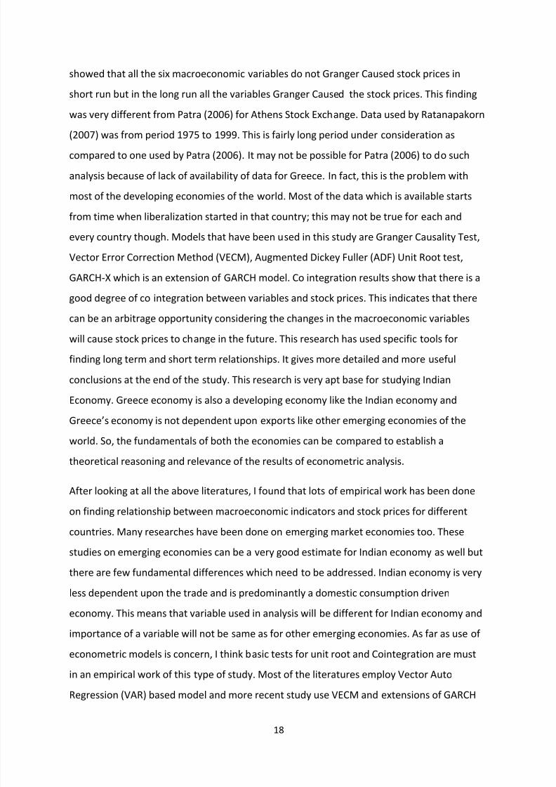
showed that all the six macroeconomic variables do not Granger Caused stock prices in
short run but in the long run all the variables Granger Caused the stock prices. This finding
was very different from Patra (2006) for Athens Stock Exchange. Data used by Ratanapakorn
(2007) was from period 1975 to 1999. This is fairly long period under consideration ascompared to one used by Patra (2006). It may not be possible for Patra (2006) to do such
analysis because of lack of availability of data for Greece. In fact, this is the problem with
most of the developing economies of the world. Most of the data which is available starts
from time when liberalization started in that country; this may not be true for each and
every country though. Models that have been used in this study are Granger Causality Test,
Vector Error Correction Method (VECM), Augmented Dickey Fuller (ADF) Unit Root test,
GARCH-X which is an extension of GARCH model. Co integration results show that there is a
good degree of co integration between variables and stock prices. This indicates that there
can be an arbitrage opportunity considering the changes in the macroeconomic variables
will cause stock prices to change in the future. This research has used specific tools for
finding long term and short term relationships. It gives more detailed and more useful
conclusions at the end of the study. This research is very apt base for studying Indian
Economy. Greece economy is also a developing economy like the Indian economy and
Greece’s economy is not dependent upon exports like other emerging economies of the
world. So, the fundamentals of both the economies can be compared to establish a
theoretical reasoning and relevance of the results of econometric analysis.
After looking at all the above literatures, I found that lots of empirical work has been done
on finding relationship between macroeconomic indicators and stock prices for different
countries. Many researches have been done on emerging market economies too. These
studies on emerging economies can be a very good estimate for Indian economy as well but
there are few fundamental differences which need to be addressed. Indian economy is very
less dependent upon the trade and is predominantly a domestic consumption driven
economy. This means that variable used in analysis will be different for Indian economy and
importance of a variable will not be same as for other emerging economies. As far as use of
econometric models is concern, I think basic tests for unit root and Cointegration are must
in an empirical work of this type of study. Most of the literatures employ Vector Auto
Regression (VAR) based model and more recent study use VECM and extensions of GARCH
8/6/2019 Long Term and Shrt Run relationship between Macroeconomic variables and stock market in India
http://slidepdf.com/reader/full/long-term-and-shrt-run-relationship-between-macroeconomic-variables-and-stock 19/48
19
model. Another very important method which is used in almost all the study was Granger
causality test but there is two more tests which I think are more informative and gives a
clearer picture of long run and short run relationships; these methods are Variance
Decomposition and Impulse Response. Although not all the research works use these twomethods but they are employed very often to check the consistency of the results obtained
by other models. There is scope of doing univariate analysis too with multivariate analysis.
Univariate analysis can be used to forecast the price of stock prices and then it can be
compared with forecast of multivariate analysis to see if we get same or different result.
Amount of difference in the result can also tell us that macroeconomic indicators which we
chose are how much efficient in deciding the movement of stock prices. All these literatures
provide a very good base for understanding the methodologies to use. They also give
information regarding which model is how much efficient in reaching conclusion. There are
conflicting results in the literatures but they are probably due to the fact that the countries
used in the studies are different and they have different economic fundamentals.
(3) THEORETICAL FRAMEWORK
Economic Variables which will be used in this research are Inflation, Interest rates, exchange
rates, Industrial Production and Money Supply. These economic variables are supposed to
be important indicators of stock Growth (see Fama 1981; Chan et al., 1986; Smith and Sims,
1993, etc.). Understanding of the cause and effect relationship of various variables with
stock Growth is very important for framing the economic policies for a country.
(3.1) Inflation
Inflation has negative relationship with stock prices; this can be seen in various researches
like Malkiel (1979). Chaudhary (2001) found positive relationship between stock prices and
inflation in economies like Argentina, Chile, Mexico and Venezuela. Lee (1992) tried to
explain this relationship using VAR and VECM models for US. He found that stock prices do
not explain variation in inflation much but interest rates do explain the variation in inflation.
The relationship between stock prices and inflation has always been a debatable issue
8/6/2019 Long Term and Shrt Run relationship between Macroeconomic variables and stock market in India
http://slidepdf.com/reader/full/long-term-and-shrt-run-relationship-between-macroeconomic-variables-and-stock 20/48
20
among the researchers. Negative relationship between stock prices and Inflation may be
due to the fact that more inflation means that currency of that country losing its value
which may cause foreign investors to withdraw money from that country and move to some
other country. But this has not always been true. We can often seen period of high inflationand stock prices rise in emerging economies. India and China are the most recent example
to this. So, though some studies prove the negative relationship but we need to look into
the other factors also.
(3.2) Exchange rate
Exchange rate is also an important variable in this research. Exchange rates can affect the
profits of a company and hence, affect the price of its stock. Abdalla and Murinde (1997)
used Granger Causality and co integration test to find that there exists a unidirectional
causality between exchange rate and stock price in developing countries like India, Pakistan
and Korea. A study done by Granger, Huang and Yang (2000) on nine Asian countries
showed different results for different countries. Impact of Exchange Rates can be on either
side. If a country is export dominant then fall in exchange rate will cause stock prices to go
up as the firms will have more profitability from exchange rates but if a country is import
dominant then increase in exchange rates will cause firms to buy at higher prices, thus
reducing their profitability and resulting in fall of stock prices.
(3.3) Interest Rate
Interest Rates causes stock prices to move in opposite direction in both long and short run.
A decrease in interest rate may in increase the profitability of a company by reducing itscosts. This may result in rise in stock prices (Ratanapakorn, 2007). A study done by
Mukherjee and Naka (1995) shows that there is a direct relation between stock prices and
short term interest rates in Japan.
(3.4) Money Supply
8/6/2019 Long Term and Shrt Run relationship between Macroeconomic variables and stock market in India
http://slidepdf.com/reader/full/long-term-and-shrt-run-relationship-between-macroeconomic-variables-and-stock 21/48
21
M3 can be said to be the amount of money in hands of people in an economy. M3 gives us a
measure of action taken by Central Bank of a country to regulate the money supply in the
economy, RBI in case of India. How do these measures affect the stock prices? This can be
estimated by the help of the M3. Increase in money can cause stock market to move upbecause as the money supply increases, the interest rates will fall and this will raise the
stock prices. Also the fact, that increase in money supply will increase the expected inflation
and hence increase the discount rates which can cause stock prices to fall. This makes
money supply a debatable topic for researchers. Ratanapakorn, O. et al (2007).
(3.5) Industrial Production
Industrial Production is a measure of how an economy is doing. If industrial production of an
economy is increasing then its stock must move up as the valuation of the firms and
businesses in that economy goes up. If IP figures of an economy are good then stock
markets tend to give good Return.
(4) EMPIRICAL FRAMEWORK
In this research, variables used are monthly average prices of BSE (SENSEX), Inflation (INF),
Industrial Production (IP), Exchange Rate (EX), Interest Rates (IR) and Money Supply (MS).
Here inflation and IP represents goods market and IR and MS represent money market.
Econometric tests and models used are Augmented Dickey Fuller, Granger Causality, Engle-
Granger Cointegration Technique, VAR analysis using Impulse Response and Variance
Decomposition. These tests and models are explained below:
(4.1)Stationary and Non stationary Data: We must check stationarity of our time series
data before using it in our models. Data is considered to be non-stationary if its first three
moments namely mean, variance and covariance are not constant. If a time series is non
stationary then it moves away from its mean value, whereas if a series is stationary then it
comes back to mean value after going up or down. Non stationary data can be made
stationary by differencing it. But this doesn’t mean that first differenced series will be
stationary. We may need second or third or even more difference depending upon the data.
Hypothesis for testing stationarity is presence of Unit Root. A series with unit root present in
8/6/2019 Long Term and Shrt Run relationship between Macroeconomic variables and stock market in India
http://slidepdf.com/reader/full/long-term-and-shrt-run-relationship-between-macroeconomic-variables-and-stock 22/48
22
it is said to be non stationary and a series where no unit root is present is said to be a
stationary series.
Studies done in the past have found that if a unit root is present in a series then that will
lead to spurious regression. Spurious regression may cause wrong results as the results
show strong relationship between the variables which may not necessarily be the case. If
this happens then we may reach to a wrong or meaningless conclusion. There are many
methods to test unit roots:
Dickey Fuller
Augmented Dickey Fuller
Philips-Perron (PP) Test
In this paper ADF has been to use as this is the most commonly used unit root test by
econometricians.
(4.2)Augmented Dickey Fuller: ADF is the augmented form of Dickey Fuller Test. This test is
used for checking the presence of unit root. ADF is used for complicated time series data.
ADF is used in following type of models
∆ = + + −1 + 1∆−1 +⋯+ ∆− +
Where is a constant, is coefficient of time trend and p is the lag order of autoregressive
process. This means that ADF allows high order autoregressive processes. To find which
order to use in a ADF, we can do the regression and see which coefficients are significant or
alternatively we can use any of the information criterion like Akaike Information Criterion,
Bayesian information criterion or Hannan Quinn information criterion. Unit root test
hypothesis is:
0: = 0 Unit Root Present
0: < 0 No Unit Root
(4.3) Cointegration Theory and Engle Granger Cointegration Test: Two series are said to be
cointegrated if they have unit root present individually in each of them and their linear
8/6/2019 Long Term and Shrt Run relationship between Macroeconomic variables and stock market in India
http://slidepdf.com/reader/full/long-term-and-shrt-run-relationship-between-macroeconomic-variables-and-stock 23/48
23
combination has lower order of integration. This theory was developed first by Engle and
Granger (1987). If we have and as non stationary series of I(1) and on regressing on
:
= +
we find that ~ I(0) then these two series are said to be cointegrated of order one. This is
precisely the Engle Granger Test. Engle Granger Cointegration technique firstly requires a
Unit Root Test to check whether the considered series are stationary or not. This unit root
test can be performed using Augmented Dickey Fuller or Philips Perron (PP) test. Co
integration technique is used to find long term relationship between the macroeconomic
variables and stock Growth.
(4.4) Granger Causality: Engle and Granger (1987) said that in two series are cointegrated
then there must be some causality between them. If we have two series and and we
regress on its lag and the lags of variable, then if coefficient of the regression are
jointly significant then we say that granger causes . Granger causality is used to find
short run and long run causal relationship. It helps in understanding the relationship in 4
ways namely
Unidirectional causality from macroeconomic variables to stock Growth,
Unidirectional causality from stock return to macroeconomic variables,
Bidirectional causality,
No relationship.
To test the hypothesis that X granger causes Y we look at following regressions:
= 1−1 + 1−1 + (Unrestricted Regression)
= 2−1 + (Restricted Regression)
To test the null hypothesis that ‘X does not cause Y’ we perform a F-Test:
8/6/2019 Long Term and Shrt Run relationship between Macroeconomic variables and stock market in India
http://slidepdf.com/reader/full/long-term-and-shrt-run-relationship-between-macroeconomic-variables-and-stock 24/48
24
=
( −)( − )
( − )
Where n is the number of observations and k is the number of estimable parameters in each
regression.
To find the causal relationship between stock prices and macroeconomic variables following
equation has been used:
=
0 +
1
=1 −+
2
=1 −+
3
=1 −
+4
=13−+5
=1− +
If the coefficient of any of the lagged macroeconomic variable is jointly significant then we
can say that the variable Granger causes the stock return.
(4.5) Vector Auto Regression (VAR): In VAR equation for each variable explains the
evolution of that variable based on its own lag and lag of other variables which are included
in the model. This study uses 5 macroeconomic variables to model VAR. The equation for
VAR is given by:
= 0 +
=1 − +
Here, = 5 × 1
0 = 5 × 1 , = 5 × 5 ,
= 5 × 1
8/6/2019 Long Term and Shrt Run relationship between Macroeconomic variables and stock market in India
http://slidepdf.com/reader/full/long-term-and-shrt-run-relationship-between-macroeconomic-variables-and-stock 25/48
25
Vector Auto Regression (VAR) is used to find the relationships between various variables by
taking into account the feedback by other variables. Estimation based on VAR includes
endogenous as well as exogenous variables in the equation making it an important tool for
multivariate analysis.
It is very important for the order of integration of all the variables used in model to be
same. If variables are I(0) then it is said to be VAR at level. If variables are I(d) where d>0
then we have to add a error correction term into our model. This type of model is called
VECM (Vector error correction model). If variables are not cointegrated and are I(d) then we
have VAR at difference. While selecting the lags for the VAR model following three
Information Criterions have been employed:
Akaike Information Criterion: It was proposed by Hirotsugu Akaike in 1974. It is used to find
the goodness of fit of any econometric model. It basically tells us about the amount of
information lost while a model is being used to describe the reality. Generalized form of AIC
can be written as:
= 2 − 2ln ()
Where k is the number of parameters in the statistical model, L is maximised value of
likelihood function for the estimated model. AIC not only measures the goodness of a fit but
it also punishes for the increased number of estimated parameter. So it can be said that AIC
discourages the over fitting. Value assigned by the AIC is meant only to ranks the model and
find the best from different models. The value is nowhere used in our estimation or
Hypothesis at any point. Model with the least value of AIC is said to be the best model.
Bayesian Information Criterion or Schwartz Information Criterion: This criterion used forsame purpose but it penalizes more for including extra parameter in model than AIC. While
using maximum likelihood estimation for estimating a model, it is possible to increase the
likelihood by adding the parameters but this may lead to over fitting. By using BIC we can
resolve this problem because BIC introduces a penalty term. As in AIC, model with lower
value to BIC should be chosen.
Hannan Quinn Information Criterion: It is also the measure of goodness of fit like AIC and
BIC.
8/6/2019 Long Term and Shrt Run relationship between Macroeconomic variables and stock market in India
http://slidepdf.com/reader/full/long-term-and-shrt-run-relationship-between-macroeconomic-variables-and-stock 26/48
26
Two very useful methods of examining the properties of VAR are Variance Decomposition
and Impulse Response.
(4.5.1) Variance Decomposition is also known as forecast error variance decomposition. It
explains the amount of information that each variable contributes towards the change in
other variables. It tells how an exogenous shock in some variables contributes to the
forecast error variance of other variable. Order of selecting the variables is an important
issue in variance decomposition. We employ Cholesky Decomposition to decide the order of
the included variables.
(4.5.2) Impulse Response is basically the graphical representation of the change caused to
other variables by the shock or impulse in one variable. This is shock in error term of one
equation which propagates into the entire system. We can also say that, we trace the
response of endogenous variables to a ‘unit’ change of error term of a particular equation.
Numerous methods can be employed to know what kind of unit change we need to make
into the system but generally we make use of positive change of one standard deviation.
This change propagates into the system and changes the value of the dependent variables
for each time period.
All the data is collected from Datastream and PCgive statistical package will be used for
calculation. Data used for the analysis will be from 1991 to 2010 which is comparatively
short period for finding the long run relationship between the variables. For long run
analysis we should have data of past 30 years at least but due to unavailability of data
before 1991 we are restricted to consider data from 1991 only.
(5.0) Tests and Results
Test for stationarity of all the series used in our analysis namely BSE, INF, EX, IR, IP, M3 is
done using Augmented Dickey Fuller Test (ADF). The results show that all of the series
contain unit root except M3 and IP. So we conclude here that M3 and IP cannot be
cointegrated with other variables because for a series to be cointegrated with other series
should be at least integrated to first order, I(1) and hence, it can be said that M3 and IP has
no long run relationship with other variables. IP is stationary at 5% significance level but it is
8/6/2019 Long Term and Shrt Run relationship between Macroeconomic variables and stock market in India
http://slidepdf.com/reader/full/long-term-and-shrt-run-relationship-between-macroeconomic-variables-and-stock 27/48
27
non stationary at 10% significance level. We would not consider 10% level significance in
this study as this may lead to misguided results in the end. For rest of the variables, they are
I(1) and we proceed with Cointegration test on them. Results for ADF test are shown in
Table 1.
Table 1:
Variable Coefficient t-statistic Variable Coefficient t-static
BSE 0.0059 1.2026 INF -0.0071 -0.9251
EX 0.0018 1.4220 IP** 0.0089 2.7785
M3 0.0135 8.8012 IR -0.0008 -0.257
**significant at 10%. Coefficient being significant means we reject the null hypothesis that unit root is present.
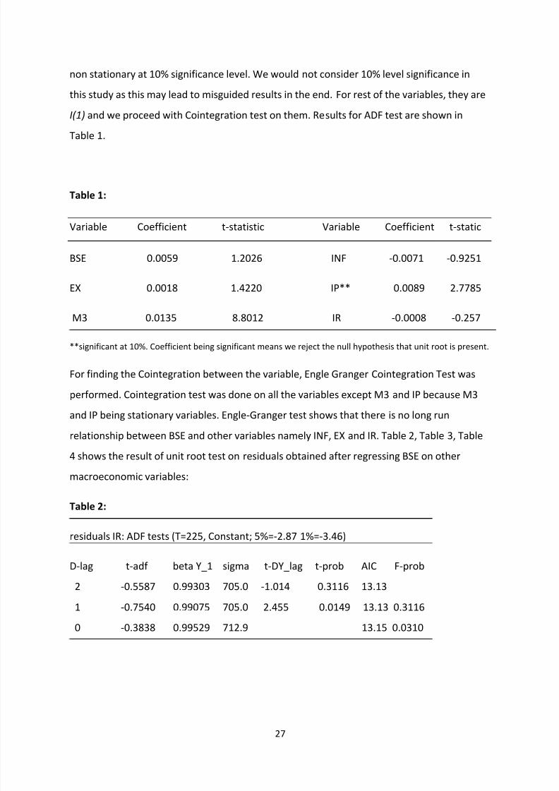
For finding the Cointegration between the variable, Engle Granger Cointegration Test was
performed. Cointegration test was done on all the variables except M3 and IP because M3
and IP being stationary variables. Engle-Granger test shows that there is no long run
relationship between BSE and other variables namely INF, EX and IR. Table 2, Table 3, Table
4 shows the result of unit root test on residuals obtained after regressing BSE on other
macroeconomic variables:
Table 2:
residuals IR: ADF tests (T=225, Constant; 5%=-2.87 1%=-3.46)
D-lag t-adf beta Y_1 sigma t-DY_lag t-prob AIC F-prob
2 -0.5587 0.99303 705.0 -1.014 0.3116 13.13
1 -0.7540 0.99075 705.0 2.455 0.0149 13.13 0.3116
0 -0.3838 0.99529 712.9 13.15 0.0310
8/6/2019 Long Term and Shrt Run relationship between Macroeconomic variables and stock market in India
http://slidepdf.com/reader/full/long-term-and-shrt-run-relationship-between-macroeconomic-variables-and-stock 28/48
28
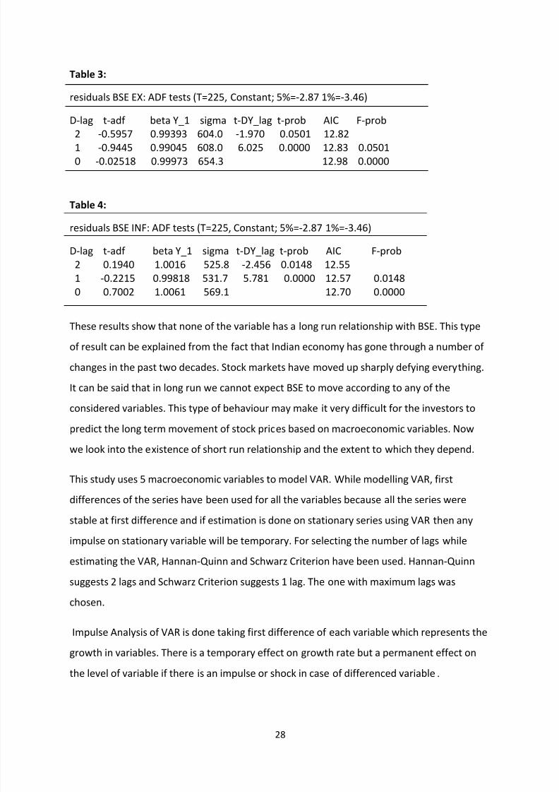
Table 3:
residuals BSE EX: ADF tests (T=225, Constant; 5%=-2.87 1%=-3.46)
D-lag t-adf beta Y_1 sigma t-DY_lag t-prob AIC F-prob
2 -0.5957 0.99393 604.0 -1.970 0.0501 12.821 -0.9445 0.99045 608.0 6.025 0.0000 12.83 0.0501
0 -0.02518 0.99973 654.3 12.98 0.0000
Table 4:
residuals BSE INF: ADF tests (T=225, Constant; 5%=-2.87 1%=-3.46)
D-lag t-adf beta Y_1 sigma t-DY_lag t-prob AIC F-prob
2 0.1940 1.0016 525.8 -2.456 0.0148 12.55
1 -0.2215 0.99818 531.7 5.781 0.0000 12.57 0.01480 0.7002 1.0061 569.1 12.70 0.0000
These results show that none of the variable has a long run relationship with BSE. This type
of result can be explained from the fact that Indian economy has gone through a number of
changes in the past two decades. Stock markets have moved up sharply defying everything.
It can be said that in long run we cannot expect BSE to move according to any of the
considered variables. This type of behaviour may make it very difficult for the investors to
predict the long term movement of stock prices based on macroeconomic variables. Now
we look into the existence of short run relationship and the extent to which they depend.
This study uses 5 macroeconomic variables to model VAR. While modelling VAR, first
differences of the series have been used for all the variables because all the series were
stable at first difference and if estimation is done on stationary series using VAR then any
impulse on stationary variable will be temporary. For selecting the number of lags while
estimating the VAR, Hannan-Quinn and Schwarz Criterion have been used. Hannan-Quinn
suggests 2 lags and Schwarz Criterion suggests 1 lag. The one with maximum lags was
chosen.
Impulse Analysis of VAR is done taking first difference of each variable which represents the
growth in variables. There is a temporary effect on growth rate but a permanent effect on
the level of variable if there is an impulse or shock in case of differenced variable.
8/6/2019 Long Term and Shrt Run relationship between Macroeconomic variables and stock market in India
http://slidepdf.com/reader/full/long-term-and-shrt-run-relationship-between-macroeconomic-variables-and-stock 29/48
29
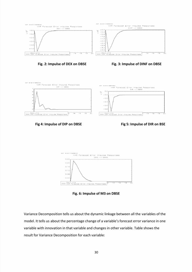
Innovations in growth of exchange rate, Inflation and Interest rates cause stock Growth to
fall of the stock prices and stock prices are set at a new level after the innovation.
In case of exchange rates and Inflation, the stock Growth take approximately 6 periods to
return to zero level, which means growth of stock prices become as they were before the
shock in 6 months. Negative effect of innovation in exchange rate on stock market is
according to the fact that India is an import dominant country and exchange rate should
have negative relationship with stock market. Shock in inflation can cause markets to go
down. This is according to the findings of Malkiel (1979).
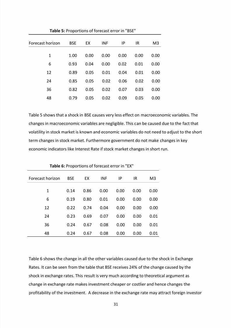
Shock caused due to Interest Rates take even less time, 4 to 5 months, for stock Growth to
come back to zero line. Effect of an innovation in Interest rates is negative on stock Growth.
These inferences are according to the functioning of an economy and can be explained
theoretically. Increase in interest rates makes it costlier for investors and businesses to
borrow for investment. Hence they move to other low interest destinations.
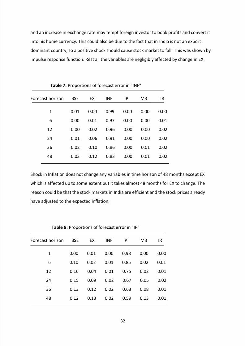
An impulse on growth of Industrial Production and Money Supply cause stock growth to
increase for sometime but the level of stock prices increase permanently. It takes almost 6
to 7 months for stock Growth to come back to zero line. This is according to the predicted
theoretical behaviour because increase in Industrial Production and Money supply means
more profit for the firms and more money in hands of people to spend. Hence this should
lead to an increase in stock growth.
These impulse responses gives us direction of the movement of stock prices with respect to
the shock in macroeconomic variables but the responses are of very small magnitude
(except for EX). So, based on these results, it can’t be said that there is a very strong
evidence of relationship between stock prices and macroeconomic variables. In fact, only EX
seem to be cause substantial movement in stock prices and rest other variables can be said
to have a negligible effect on stock growth. Results of Impulse response are show in figures
below:
8/6/2019 Long Term and Shrt Run relationship between Macroeconomic variables and stock market in India
http://slidepdf.com/reader/full/long-term-and-shrt-run-relationship-between-macroeconomic-variables-and-stock 30/48
30
Fig. 2: Impulse of DEX on DBSE Fig. 3: Impulse of DINF on DBSE
Fig 4: Impulse of DIP on DBSE Fig 5: Impulse of DIR on BSE
Fig. 6: Impulse of M3 on DBSE
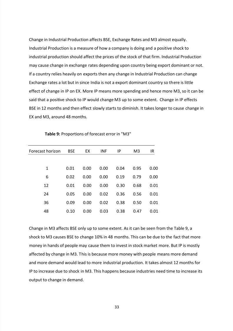
Variance Decomposition tells us about the dynamic linkage between all the variables of the
model. It tells us about the percentage change of a variable’s forecast error variance in one
variable with innovation in that variable and changes in other variable. Table shows the
result for Variance Decomposition for each variable:
8/6/2019 Long Term and Shrt Run relationship between Macroeconomic variables and stock market in India
http://slidepdf.com/reader/full/long-term-and-shrt-run-relationship-between-macroeconomic-variables-and-stock 31/48
31
Table 5: Proportions of forecast error in "BSE"
Forecast horizon BSE EX INF IP IR M3
1 1.00 0.00 0.00 0.00 0.00 0.006 0.93 0.04 0.00 0.02 0.01 0.00
12 0.89 0.05 0.01 0.04 0.01 0.00
24 0.85 0.05 0.02 0.06 0.02 0.00
36 0.82 0.05 0.02 0.07 0.03 0.00
48 0.79 0.05 0.02 0.09 0.05 0.00
Table 5 shows that a shock in BSE causes very less effect on macroeconomic variables. The
changes in macroeconomic variables are negligible. This can be caused due to the fact that
volatility in stock market is known and economic variables do not need to adjust to the short
term changes in stock market. Furthermore government do not make changes in key
economic indicators like Interest Rate if stock market changes in short run.
Table 6: Proportions of forecast error in "EX"
Forecast horizon BSE EX INF IP IR M3
1 0.14 0.86 0.00 0.00 0.00 0.00
6 0.19 0.80 0.01 0.00 0.00 0.00
12 0.22 0.74 0.04 0.00 0.00 0.00
24 0.23 0.69 0.07 0.00 0.00 0.01
36 0.24 0.67 0.08 0.00 0.00 0.01
48 0.24 0.67 0.08 0.00 0.00 0.01
Table 6 shows the change in all the other variables caused due to the shock in Exchange
Rates. It can be seen from the table that BSE receives 24% of the change caused by the
shock in exchange rates. This result is very much according to theoretical argument as
change in exchange rate makes investment cheaper or costlier and hence changes the
profitability of the investment. A decrease in the exchange rate may attract foreign investor
8/6/2019 Long Term and Shrt Run relationship between Macroeconomic variables and stock market in India
http://slidepdf.com/reader/full/long-term-and-shrt-run-relationship-between-macroeconomic-variables-and-stock 32/48
32
and an increase in exchange rate may tempt foreign investor to book profits and convert it
into his home currency. This could also be due to the fact that in India is not an export
dominant country, so a positive shock should cause stock market to fall. This was shown by
impulse response function. Rest all the variables are negligibly affected by change in EX.
Table 7: Proportions of forecast error in "INF"
Forecast horizon BSE EX INF IP M3 IR
1 0.01 0.00 0.99 0.00 0.00 0.00
6 0.00 0.01 0.97 0.00 0.00 0.01
12 0.00 0.02 0.96 0.00 0.00 0.02
24 0.01 0.06 0.91 0.00 0.00 0.02
36 0.02 0.10 0.86 0.00 0.01 0.02
48 0.03 0.12 0.83 0.00 0.01 0.02
Shock in Inflation does not change any variables in time horizon of 48 months except EX
which is affected up to some extent but it takes almost 48 months for EX to change. The
reason could be that the stock markets in India are efficient and the stock prices already
have adjusted to the expected inflation.
Table 8: Proportions of forecast error in "IP"
Forecast horizon BSE EX INF IP M3 IR
1 0.00 0.01 0.00 0.98 0.00 0.00
6 0.10 0.02 0.01 0.85 0.02 0.01
12 0.16 0.04 0.01 0.75 0.02 0.01
24 0.15 0.09 0.02 0.67 0.05 0.02
36 0.13 0.12 0.02 0.63 0.08 0.01
48 0.12 0.13 0.02 0.59 0.13 0.01
8/6/2019 Long Term and Shrt Run relationship between Macroeconomic variables and stock market in India
http://slidepdf.com/reader/full/long-term-and-shrt-run-relationship-between-macroeconomic-variables-and-stock 33/48
33
Change in Industrial Production affects BSE, Exchange Rates and M3 almost equally.
Industrial Production is a measure of how a company is doing and a positive shock to
industrial production should affect the prices of the stock of that firm. Industrial Productionmay cause change in exchange rates depending upon country being export dominant or not.
If a country relies heavily on exports then any change in Industrial Production can change
Exchange rates a lot but in since India is not a export dominant country so there is little
effect of change in IP on EX. More IP means more spending and hence more M3, so it can be
said that a positive shock to IP would change M3 up to some extent. Change in IP effects
BSE in 12 months and then effect slowly starts to diminish. It takes longer to cause change in
EX and M3, around 48 months.
Table 9: Proportions of forecast error in "M3"
Forecast horizon BSE EX INF IP M3 IR
1 0.01 0.00 0.00 0.04 0.95 0.00
6 0.02 0.00 0.00 0.19 0.79 0.00
12 0.01 0.00 0.00 0.30 0.68 0.01
24 0.05 0.00 0.02 0.36 0.56 0.01
36 0.09 0.00 0.02 0.38 0.50 0.01
48 0.10 0.00 0.03 0.38 0.47 0.01
Change in M3 affects BSE only up to some extent. As it can be seen from the Table 9, a
shock to M3 causes BSE to change 10% in 48 months. This can be due to the fact that more
money in hands of people may cause them to invest in stock market more. But IP is mostly
affected by change in M3. This is because more money with people means more demand
and more demand would lead to more industrial production. It takes almost 12 months for
IP to increase due to shock in M3. This happens because industries need time to increase its
output to change in demand.
8/6/2019 Long Term and Shrt Run relationship between Macroeconomic variables and stock market in India
http://slidepdf.com/reader/full/long-term-and-shrt-run-relationship-between-macroeconomic-variables-and-stock 34/48
34
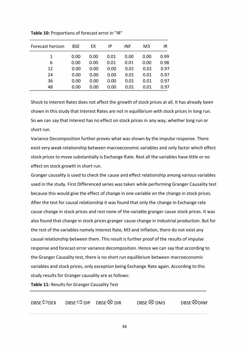
Table 10: Proportions of forecast error in "IR"
Forecast horizon BSE EX IP INF M3 IR
1 0.00 0.00 0.01 0.00 0.00 0.99
6 0.00 0.00 0.01 0.01 0.00 0.9812 0.00 0.00 0.00 0.01 0.01 0.97
24 0.00 0.00 0.00 0.01 0.01 0.97
36 0.00 0.00 0.00 0.01 0.01 0.97
48 0.00 0.00 0.00 0.01 0.01 0.97
Shock to Interest Rates does not affect the growth of stock prices at all. It has already been
shown in this study that Interest Rates are not in equilibrium with stock prices in long run.
So we can say that Interest has no effect on stock prices in any way, whether long run or
short run.
Variance Decomposition further proves what was shown by the impulse response. There
exist very weak relationship between macroeconomic variables and only factor which effect
stock prices to move substantially is Exchange Rate. Rest all the variables have little or no
effect on stock growth in short run.
Granger causality is used to check the cause and effect relationship among various variables
used in the study. First Differenced series was taken while performing Granger Causality test
because this would give the effect of change in one variable on the change in stock prices.
After the test for causal relationship it was found that only the change in Exchange rate
cause change in stock prices and rest none of the variable granger cause stock prices. It was
also found that change in stock prices granger cause change in Industrial production. But for
the rest of the variables namely Interest Rate, M3 and Inflation, there do not exist any
causal relationship between them. This result is further proof of the results of impulse
response and forecast error variance decomposition. Hence we can say that according to
the Granger Causality test, there is no short run equilibrium between macroeconomic
variables and stock prices, only exception being Exchange Rate again. According to this
study results for Granger causality are as follows:
Table 11: Results for Granger Causality Test
DBSE DEX DBSE DIP DBSE DIR DBSE DM3 DBSE DINF
8/6/2019 Long Term and Shrt Run relationship between Macroeconomic variables and stock market in India
http://slidepdf.com/reader/full/long-term-and-shrt-run-relationship-between-macroeconomic-variables-and-stock 35/48
35
6.0 ConclusionThis dissertation is aimed to find the long run equilibrium and the short run dynamic
relationship between Indian stock prices and its macroeconomic variables. This study shows
that there is no long run equilibrium between macroeconomic variables and stock prices.
This means that in long run stock prices do not adjust for the change in macroeconomic
variables. This behaviour is very rare, not seen in many economies. Possible reason for such
behaviour can be the fact that Indian economy has been very volatile in past 20 years. None
of the variables have been stable in past. Another reason could be that data used in this
study is only 20 year old. A longer time frame could have shown much clearer picture of the
long run equilibrium between macroeconomic variables and stock prices but due to the
constraints of availability of data, only past 20 years were taken into consideration in this
study. Results of short run dynamic relationship between macroeconomic variables and
stock prices too show that macroeconomic variables affect Indian stock prices up to very
small extent. The only exception is Exchange Rate which can be said to have a short run
relationship with stock prices. Rest all the variables effect stock prices but very little.
Impulse response proves that EX, INF and IR cause BSE to change negatively and M3 and IP
change stock prices in same direction as the impulse. These results are further consolidated
by the outcomes from Forecast Error Variance Decomposition and Granger Causality. These
results show that Indian stock prices do not depend on macroeconomic variables. It can be
said that Indian stock market depends more on international events and other stock
markets than the domestic factors like macroeconomic situations. In recent years Indian
stock markets have become more integrated with stock markets of big economies like US
and UK. Due to this integration the markets are more affected by the broader events of
world economies than the domestic economy. Another reason for such results may be the
fact that Indian economy is driven mostly by domestic consumption and in the past 20 years
there has been a steep rise in Indian middle class which has caused domestic consumption
to increase multiple times. This phenomenon might have over shadowed the other
macroeconomic events. This also shows that it may be very difficult for government tocontrol stock prices from going down or up using macroeconomic variables and hence

8/6/2019 Long Term and Shrt Run relationship between Macroeconomic variables and stock market in India
http://slidepdf.com/reader/full/long-term-and-shrt-run-relationship-between-macroeconomic-variables-and-stock 36/48
36
government would be left with options such as applying cap on amount of foreign indirect
investments into the country. In past, Indian government have in fact capped many sectors
from foreign direct investments and foreign indirect investments.
Further study in this field may to look into the specific sectors of Indian economy and see if stock prices, of these sectors, are affected by the change in macroeconomic variables.
Another direction of study may be to include other factors which can affect stock prices like
US stock exchange prices, crude oil price, etc.
8/6/2019 Long Term and Shrt Run relationship between Macroeconomic variables and stock market in India
http://slidepdf.com/reader/full/long-term-and-shrt-run-relationship-between-macroeconomic-variables-and-stock 37/48
37
7.0 References:
Abdalla, I. S. A. and Murinde, V. (1997) Exchange rate and stock price interactions in
emerging financial markets: evidence on India, Korea, Pakistan and the Philippines,
Applied Financial Economics, 7, 25 –35.
Abdullah, D.A. and S.C. Hayworth, Macroeconomics of stock price fluctuations. Quarterly
Journal of Business & Economics, 1993. 32(1): p. 50.
Bekaert, G., et al., Distributional characteristics of emerging market returns and asset
allocation. Journal of Portfolio Management, 1998. 24(2): p. 102-+.
Chen, N. F., Roll, R. and Ross, S. (1986) Economic forces and the stock market , Journal of
Business, 59, 383 –403.
Choudhary, T. (2001) Inflation and rates of return on stocks: evidence from high inflation
countries, Journal of International Financial Markets, Institutions and Money, 11, 75 –96.
Engle, R. and Granger, C. W. S. (1987) Cointegration and error correction: representation
estimation and testing, Econometrica, 55, 251 –76.
Fama, E. (1981) Stock return, real activity, inflation and money , American Economic
Review, 65, 269 –82.
Fama, E., The behaviour of stock market prices, Journal of Business, 1965, 38, p. 34 –105.
Granger, C. W. and Morgerstern, O., Spectral Analysis of New York stock market prices,
Kyklos, 1963, 16, p.1 –27.
8/6/2019 Long Term and Shrt Run relationship between Macroeconomic variables and stock market in India
http://slidepdf.com/reader/full/long-term-and-shrt-run-relationship-between-macroeconomic-variables-and-stock 38/48
38
Granger, C. W., Huang, B. N. and Yang, C. W. (2000) A bivariate causality between stock
prices and exchange rates: evidence from recent Asian flu, The Quarterly Review of
Economics and Finance, 40, 337 –54.
Granger, C. W., Some recent developments in the concept of causality , Journal of
Econometrics, 1986, 39, p. 194 –211.
Ibrahim, M.H., MACROECONOMIC FORCES AND CAPITAL MARKET INTEGRATION. Journal
of the Asia Pacific Economy, 2003. 8(1): p. 19.
Kwon, C.S. and T.S. Shin, Cointegration and causality between macroeconomic variables
and stock market returns. Global Finance Journal, 1999. 10(1): p. 71.
Malkiel, B (1979), the capital formation problem in the, United States, Journal of Finance,
34, p. 291 –306.
Muradoglu, G., F. Taskin, and I. Bigan, Causality Between Stock Returns and
Macroeconomic Variables in Emerging Markets. Russian & East European Finance &
Trade, 2000. 36(6): p. 33.
Patra, T. and S. Poshakwale, Economic variables and stock market returns: evidence from
the Athens stock exchange. Applied Financial Economics, 2006. 16(13): p. 993-1005.
Ratanapakorn, O. and S.C. Sharma, Dynamic analysis between the US stock returns and
the macroeconomic variables. Applied Financial Economics, 2007. 17(5): p. 369-377.
Smith, K. and Sims, A. (1993) Stock market performance and macroeconomic variables,
Applied Financial Economics, 3, 55 –60.
8/6/2019 Long Term and Shrt Run relationship between Macroeconomic variables and stock market in India
http://slidepdf.com/reader/full/long-term-and-shrt-run-relationship-between-macroeconomic-variables-and-stock 39/48
39
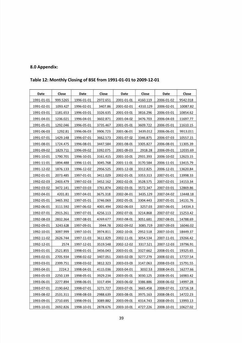
8.0 Appendix:
Table 12: Monthly Closing of BSE from 1991-01-01 to 2009-12-01
Date Close Date Close Date Close Date Close
1991-01-01 999.5265 1996-01-01 2972.651 2001-01-01 4160.119 2006-01-02 9542.018
1991-02-01 1093.427 1996-02-01 3407.86 2001-02-01 4310.129 2006-02-01 10087.82
1991-03-01 1181.653 1996-03-01 3326.635 2001-03-01 3816.296 2006-03-01 10854.62
1991-04-01 1236.021 1996-04-01 3602.871 2001-04-02 3476.703 2006-04-03 11697.771991-05-01 1292.046 1996-05-01 3735.467 2001-05-01 3609.722 2006-05-01 11610.15
1991-06-03 1292.81 1996-06-03 3906.723 2001-06-01 3439.012 2006-06-01 9913.011
1991-07-01 1429.148 1996-07-01 3662.573 2001-07-02 3346.875 2006-07-03 10557.15
1991-08-01 1724.475 1996-08-01 3447.584 2001-08-01 3305.827 2006-08-01 11305.39
1991-09-02 1829.711 1996-09-02 3392.075 2001-09-03 2918.28 2006-09-01 12035.69
1991-10-01 1790.701 1996-10-01 3161.415 2001-10-01 2931.393 2006-10-02 12623.15
1991-11-01 1894.488 1996-11-01 3045.768 2001-11-01 3170.584 2006-11-01 13415.79
1991-12-02 1876.133 1996-12-02 2956.525 2001-12-03 3312.825 2006-12-01 13620.84
1992-01-01 2073.485 1997-01-01 3411.029 2002-01-01 3353.313 2007-01-01 13998.33
1992-02-03 2403.479 1997-02-03 3452.162 2002-02-01 3528.575 2007-02-01 14153.34
1992-03-02 3472.141 1997-03-03 3761.874 2002-03-01 3572.347 2007-03-01 12869.86
1992-04-01 4201.81 1997-04-01 3675.318 2002-04-01 3435.129 2007-04-02 13448.18
1992-05-01 3465.392 1997-05-01 3746.069 2002-05-01 3304.443 2007-05-01 14131.76
1992-06-01 3111.592 1997-06-02 4001.494 2002-06-03 3257.03 2007-06-01 14334.3
1992-07-01 2915.261 1997-07-01 4256.113 2002-07-01 3214.868 2007-07-02 15253.42
1992-08-03 2832.364 1997-08-01 4269.677 2002-08-01 3051.681 2007-08-01 14788.69
1992-09-01 3243.628 1997-09-01 3944.78 2002-09-02 3085.719 2007-09-03 16046.02
1992-10-01 3097.999 1997-10-01 3974.811 2002-10-01 2952.518 2007-10-01 18449.37
1992-11-02 2626.744 1997-11-03 3611.829 2002-11-01 3054.534 2007-11-01 19266.42
1992-12-01 2574 1997-12-01 3519.548 2002-12-02 3317.521 2007-12-03 19796.91
1993-01-01 2521.855 1998-01-01 3456.043 2003-01-01 3327.662 2008-01-01 19325.65
1993-02-01 2705.934 1998-02-02 3407.051 2003-02-03 3277.279 2008-02-01 17727.54
1993-03-01 2399.751 1998-03-02 3812.323 2003-03-03 3147.063 2008-03-03 15791.55
1993-04-01 2224.2 1998-04-01 4115.036 2003-04-01 3032.53 2008-04-01 16277.66
1993-05-03 2250.139 1998-05-01 3929.234 2003-05-01 3030.125 2008-05-01 16983.42
1993-06-01 2277.894 1998-06-01 3317.494 2003-06-02 3386.886 2008-06-02 14997.28
1993-07-01 2190.642 1998-07-01 3271.727 2003-07-01 3665.458 2008-07-01 13716.18
1993-08-02 2531.311 1998-08-03 2988.639 2003-08-01 3975.163 2008-08-01 14722.23
1993-09-01 2710.695 1998-09-01 3089.882 2003-09-01 4314.743 2008-09-01 13993.13
1993-10-01 2692.826 1998-10-01 2878.676 2003-10-01 4727.226 2008-10-01 10627.02
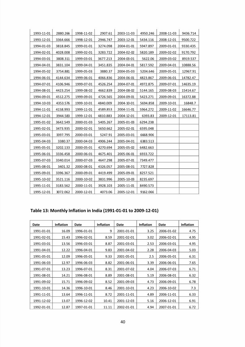
8/6/2019 Long Term and Shrt Run relationship between Macroeconomic variables and stock market in India
http://slidepdf.com/reader/full/long-term-and-shrt-run-relationship-between-macroeconomic-variables-and-stock 40/48
40
1993-11-01 2880.266 1998-11-02 2907.61 2003-11-03 4950.246 2008-11-03 9436.714
1993-12-01 3364.666 1998-12-01 2946.747 2003-12-01 5434.116 2008-12-01 9500.722
1994-01-03 3818.845 1999-01-01 3274.098 2004-01-01 5947.897 2009-01-01 9330.435
1994-02-01 4028.008 1999-02-01 3283.722 2004-02-02 5820.189 2009-02-02 9170.792
1994-03-01 3808.311 1999-03-01 3677.213 2004-03-01 5622.06 2009-03-02 8919.537
1994-04-01 3831.104 1999-04-01 3451.835 2004-04-01 5817.592 2009-04-01 10888.56
1994-05-02 3754.881 1999-05-03 3880.37 2004-05-03 5204.646 2009-05-01 12967.91
1994-06-01 4144.634 1999-06-01 4066.836 2004-06-01 4823.867 2009-06-01 14782.47
1994-07-01 4106.946 1999-07-01 4526.254 2004-07-01 4972.875 2009-07-01 14635.19
1994-08-01 4423.254 1999-08-02 4662.839 2004-08-02 5144.165 2009-08-03 15414.67
1994-09-01 4512.275 1999-09-01 4726.565 2004-09-01 5423.271 2009-09-01 16372.88
1994-10-03 4353.576 1999-10-01 4840.009 2004-10-01 5694.858 2009-10-01 16848.7
1994-11-01 4158.993 1999-11-01 4589.853 2004-11-01 5964.272 2009-11-02 16646.77
1994-12-01 3944.583 1999-12-01 4810.883 2004-12-01 6393.83 2009-12-01 17113.81
1995-01-02 3642.549 2000-01-03 5405.267 2005-01-03 6294.238
1995-02-01 3473.935 2000-02-01 5650.662 2005-02-01 6595.048
1995-03-01 3397.795 2000-03-01 5247.91 2005-03-01 6668.906
1995-04-03 3380.37 2000-04-03 4906.244 2005-04-01 6383.513
1995-05-01 3202.133 2000-05-01 4270.694 2005-05-02 6482.663
1995-06-01 3336.458 2000-06-01 4675.401 2005-06-01 6933.722
1995-07-03 3340.014 2000-07-03 4647.298 2005-07-01 7349.477
1995-08-01 3401.32 2000-08-01 4326.057 2005-08-01 7727.828
1995-09-01 3396.367 2000-09-01 4419.499 2005-09-01 8257.521
1995-10-02 3521.116 2000-10-02 3831.996 2005-10-03 8235.697
1995-11-01 3183.562 2000-11-01 3928.103 2005-11-01 8490.573
1995-12-01 3072.062 2000-12-01 4073.06 2005-12-01 9162.066
Table 13: Monthly Inflation in India (1991-01-01 to 2009-12-01)
Date Inflation Date Inflation Date Inflation Date Inflation
1991-01-01 16.09 1996-01-01 9 2001-01-01 3.25 2006-01-02 4.75
1991-02-01 15.43 1996-02-01 8.59 2001-02-01 3.02 2006-02-01 4.95
1991-03-01 13.56 1996-03-01 8.87 2001-03-01 2.53 2006-03-01 4.95
1991-04-01 12.22 1996-04-01 9.83 2001-04-02 2.28 2006-04-03 5.03
1991-05-01 12.09 1996-05-01 9.33 2001-05-01 2.5 2006-05-01 6.31
1991-06-03 12.97 1996-06-03 8.82 2001-06-01 3.39 2006-06-01 7.65
1991-07-01 13.23 1996-07-01 8.31 2001-07-02 4.04 2006-07-03 6.71
1991-08-01 14.21 1996-08-01 8.89 2001-08-01 5.19 2006-08-01 6.32
1991-09-02 15.71 1996-09-02 8.52 2001-09-03 4.73 2006-09-01 6.78
1991-10-01 14.36 1996-10-01 8.46 2001-10-01 4.23 2006-10-02 7.3
1991-11-01 13.64 1996-11-01 8.72 2001-11-01 4.89 2006-11-01 6.33
1991-12-02 13.07 1996-12-02 10.41 2001-12-03 5.16 2006-12-01 6.91
1992-01-01 12.87 1997-01-01 11.11 2002-01-01 4.94 2007-01-01 6.72
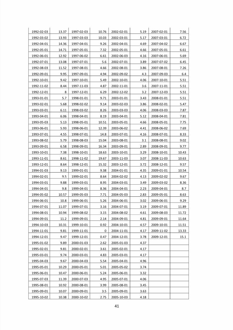
8/6/2019 Long Term and Shrt Run relationship between Macroeconomic variables and stock market in India
http://slidepdf.com/reader/full/long-term-and-shrt-run-relationship-between-macroeconomic-variables-and-stock 41/48
41
1992-02-03 13.37 1997-02-03 10.76 2002-02-01 5.19 2007-02-01 7.56
1992-03-02 13.93 1997-03-03 10.03 2002-03-01 5.17 2007-03-01 6.72
1992-04-01 14.36 1997-04-01 9.26 2002-04-01 4.69 2007-04-02 6.67
1992-05-01 14.71 1997-05-01 7.32 2002-05-01 4.66 2007-05-01 6.61
1992-06-01 12.92 1997-06-02 6.61 2002-06-03 4.16 2007-06-01 5.69
1992-07-01 13.08 1997-07-01 5.6 2002-07-01 3.89 2007-07-02 6.45
1992-08-03 11.52 1997-08-01 4.66 2002-08-01 3.86 2007-08-01 7.26
1992-09-01 9.95 1997-09-01 4.94 2002-09-02 4.3 2007-09-03 6.4
1992-10-01 9.42 1997-10-01 5.49 2002-10-01 4.06 2007-10-01 5.51
1992-11-02 8.44 1997-11-03 4.87 2002-11-01 3.6 2007-11-01 5.51
1992-12-01 8 1997-12-01 6.29 2002-12-02 3.2 2007-12-03 5.51
1993-01-01 5.7 1998-01-01 9.71 2003-01-01 3.43 2008-01-01 5.51
1993-02-01 5.68 1998-02-02 9.14 2003-02-03 3.86 2008-02-01 5.47
1993-03-01 6.11 1998-03-02 8.26 2003-03-03 4.06 2008-03-03 7.87
1993-04-01 6.06 1998-04-01 8.19 2003-04-01 5.12 2008-04-01 7.81
1993-05-03 5.13 1998-05-01 10.51 2003-05-01 4.66 2008-05-01 7.75
1993-06-01 5.93 1998-06-01 12.39 2003-06-02 4.41 2008-06-02 7.69
1993-07-01 4.55 1998-07-01 14.8 2003-07-01 4.16 2008-07-01 8.33
1993-08-02 5.79 1998-08-03 15.04 2003-08-01 3.1 2008-08-01 9.02
1993-09-01 6.58 1998-09-01 16.34 2003-09-01 2.89 2008-09-01 9.77
1993-10-01 7.38 1998-10-01 18.63 2003-10-01 3.29 2008-10-01 10.43
1993-11-01 8.61 1998-11-02 19.67 2003-11-03 3.07 2008-11-03 10.63
1993-12-01 8.64 1998-12-01 15.32 2003-12-01 3.72 2008-12-01 9.57
1994-01-03 9.13 1999-01-01 9.38 2004-01-01 4.35 2009-01-01 10.54
1994-02-01 9.5 1999-02-01 8.64 2004-02-02 4.13 2009-02-02 9.67
1994-03-01 9.88 1999-03-01 8.95 2004-03-01 3.49 2009-03-02 8.36
1994-04-01 9.8 1999-04-01 8.36 2004-04-01 2.23 2009-04-01 8.7
1994-05-02 10.57 1999-05-03 7.71 2004-05-03 2.83 2009-05-01 8.63
1994-06-01 10.8 1999-06-01 5.26 2004-06-01 3.02 2009-06-01 9.29
1994-07-01 11.07 1999-07-01 3.16 2004-07-01 3.19 2009-07-01 11.89
1994-08-01 10.94 1999-08-02 3.15 2004-08-02 4.61 2009-08-03 11.72
1994-09-01 11.2 1999-09-01 2.14 2004-09-01 4.81 2009-09-01 11.64
1994-10-03 10.31 1999-10-01 0.92 2004-10-01 4.57 2009-10-01 11.51
1994-11-01 9.81 1999-11-01 0 2004-11-01 4.17 2009-11-02 13.331994-12-01 9.47 1999-12-01 0.47 2004-12-01 3.78 2009-12-01 15.1
1995-01-02 9.89 2000-01-03 2.62 2005-01-03 4.37
1995-02-01 9.81 2000-02-01 3.61 2005-02-01 4.17
1995-03-01 9.74 2000-03-01 4.83 2005-03-01 4.17
1995-04-03 9.67 2000-04-03 5.54 2005-04-01 4.96
1995-05-01 10.29 2000-05-01 5.01 2005-05-02 3.74
1995-06-01 10.47 2000-06-01 5.24 2005-06-01 3.32
1995-07-03 11.39 2000-07-03 4.95 2005-07-01 4.06
1995-08-01 10.92 2000-08-01 3.99 2005-08-01 3.45
1995-09-01 10.07 2000-09-01 3.5 2005-09-01 3.63
1995-10-02 10.38 2000-10-02 2.75 2005-10-03 4.18
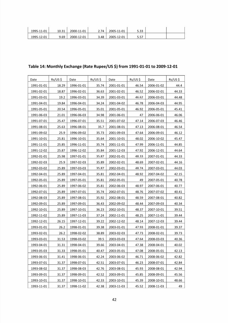
8/6/2019 Long Term and Shrt Run relationship between Macroeconomic variables and stock market in India
http://slidepdf.com/reader/full/long-term-and-shrt-run-relationship-between-macroeconomic-variables-and-stock 42/48
42
1995-11-01 10.31 2000-11-01 2.74 2005-11-01 5.33
1995-12-01 9.69 2000-12-01 3.48 2005-12-01 5.57
Table 14: Monthly Exchange (Rate Rupee/US $) from 1991-01-01 to 2009-12-01
Date Rs/US $ Date Rs/US $ Date Rs/US $ Date Rs/US $
1991-01-01 18.29 1996-01-01 35.74 2001-01-01 46.54 2006-01-02 44.4
1991-02-01 18.87 1996-02-01 36.63 2001-02-01 46.52 2006-02-01 44.33
1991-03-01 19.2 1996-03-01 34.39 2001-03-01 46.62 2006-03-01 44.48
1991-04-01 19.84 1996-04-01 34.24 2001-04-02 46.78 2006-04-03 44.95
1991-05-01 20.54 1996-05-01 35.01 2001-05-01 46.92 2006-05-01 45.41
1991-06-03 21.01 1996-06-03 34.98 2001-06-01 47 2006-06-01 46.06
1991-07-01 25.47 1996-07-01 35.51 2001-07-02 47.14 2006-07-03 46.46
1991-08-01 25.63 1996-08-01 35.7 2001-08-01 47.13 2006-08-01 46.54
1991-09-02 25.9 1996-09-02 35.73 2001-09-03 47.64 2006-09-01 46.12
1991-10-01 25.81 1996-10-01 35.64 2001-10-01 48.02 2006-10-02 45.47
1991-11-01 25.85 1996-11-01 35.74 2001-11-01 47.99 2006-11-01 44.85
1991-12-02 25.87 1996-12-02 35.84 2001-12-03 47.92 2006-12-01 44.64
1992-01-01 25.98 1997-01-01 35.87 2002-01-01 48.33 2007-01-01 44.33
1992-02-03 25.9 1997-02-03 35.89 2002-02-01 48.69 2007-02-01 44.16
1992-03-02 25.89 1997-03-03 35.87 2002-03-01 48.74 2007-03-01 44.031992-04-01 25.89 1997-04-01 35.81 2002-04-01 48.92 2007-04-02 42.15
1992-05-01 25.89 1997-05-01 35.81 2002-05-01 49 2007-05-01 40.78
1992-06-01 25.89 1997-06-02 35.81 2002-06-03 48.97 2007-06-01 40.77
1992-07-01 25.89 1997-07-01 35.74 2002-07-01 48.76 2007-07-02 40.41
1992-08-03 25.89 1997-08-01 35.92 2002-08-01 48.59 2007-08-01 40.82
1992-09-01 25.89 1997-09-01 36.43 2002-09-02 48.44 2007-09-03 40.34
1992-10-01 25.89 1997-10-01 36.23 2002-10-01 48.37 2007-10-01 39.51
1992-11-02 25.89 1997-11-03 37.24 2002-11-01 48.25 2007-11-01 39.44
1992-12-01 26.15 1997-12-01 39.22 2002-12-02 48.14 2007-12-03 39.44
1993-01-01 26.2 1998-01-01 39.38 2003-01-01 47.93 2008-01-01 39.37
1993-02-01 26.2 1998-02-02 38.89 2003-02-03 47.73 2008-02-01 39.73
1993-03-01 31.53 1998-03-02 39.5 2003-03-03 47.64 2008-03-03 40.36
1993-04-01 31.31 1998-04-01 39.66 2003-04-01 47.38 2008-04-01 40.02
1993-05-03 31.33 1998-05-01 40.47 2003-05-01 47.08 2008-05-01 42.13
1993-06-01 31.41 1998-06-01 42.24 2003-06-02 46.71 2008-06-02 42.82
1993-07-01 31.37 1998-07-01 42.51 2003-07-01 46.23 2008-07-01 42.84
1993-08-02 31.37 1998-08-03 42.76 2003-08-01 45.93 2008-08-01 42.94
1993-09-01 31.37 1998-09-01 42.52 2003-09-01 45.85 2008-09-01 45.56
1993-10-01 31.37 1998-10-01 42.33 2003-10-01 45.39 2008-10-01 48.66
1993-11-01 31.37 1998-11-02 42.38 2003-11-03 45.52 2008-11-03 49

8/6/2019 Long Term and Shrt Run relationship between Macroeconomic variables and stock market in India
http://slidepdf.com/reader/full/long-term-and-shrt-run-relationship-between-macroeconomic-variables-and-stock 43/48
43
1993-12-01 31.37 1998-12-01 42.55 2003-12-01 45.59 2008-12-01 48.63
1994-01-03 31.37 1999-01-01 42.51 2004-01-01 45.46 2009-01-01 48.83
1994-02-01 31.37 1999-02-01 42.47 2004-02-02 45.27 2009-02-02 49.26
1994-03-01 31.37 1999-03-01 42.45 2004-03-01 45.02 2009-03-02 51.23
1994-04-01 31.37 1999-04-01 42.73 2004-04-01 43.93 2009-04-01 50.06
1994-05-02 31.37 1999-05-03 42.77 2004-05-03 45.25 2009-05-01 48.53
1994-06-01 31.37 1999-06-01 43.14 2004-06-01 45.51 2009-06-01 47.77
1994-07-01 31.37 1999-07-01 43.29 2004-07-01 46.04 2009-07-01 48.48
1994-08-01 31.37 1999-08-02 43.46 2004-08-02 46.34 2009-08-03 48.34
1994-09-01 31.37 1999-09-01 43.53 2004-09-01 46.1 2009-09-01 48.44
1994-10-03 31.37 1999-10-01 43.45 2004-10-01 45.78 2009-10-01 46.72
1994-11-01 31.39 1999-11-01 43.4 2004-11-01 45.13 2009-11-02 46.57
1994-12-01 31.39 1999-12-01 43.49 2004-12-01 43.98 2009-12-01 46.63
1995-01-02 31.37 2000-01-03 43.55 2005-01-03 43.75
1995-02-01 31.38 2000-02-01 43.61 2005-02-01 43.68
1995-03-01 31.65 2000-03-01 43.59 2005-03-01 43.69
1995-04-03 31.41 2000-04-03 43.64 2005-04-01 43.74
1995-05-01 31.42 2000-05-01 43.98 2005-05-02 43.49
1995-06-01 31.4 2000-06-01 44.69 2005-06-01 43.58
1995-07-03 31.38 2000-07-03 44.78 2005-07-01 43.54
1995-08-01 31.58 2000-08-01 45.68 2005-08-01 43.62
1995-09-01 33.18 2000-09-01 45.89 2005-09-01 43.92
1995-10-02 34.54 2000-10-02 46.34 2005-10-03 44.82
1995-11-01 34.74 2000-11-01 46.78 2005-11-01 45.73
1995-12-01 34.96 2000-12-01 46.75 2005-12-01 45.64
Table 15: Monthly Industrial Production in India (1991-01-01 to 2009-12-01)
Date IP Date IP Date IP Date IP
1991-01-01 45.1 1996-01-01 61.7 2001-01-01 78.8 2006-01-02 109.3
1991-02-01 44.5 1996-02-01 60.2 2001-02-01 76.9 2006-02-01 105
1991-03-01 55.2 1996-03-01 65.7 2001-03-01 82.3 2006-03-01 116.4
1991-04-01 39.7 1996-04-01 58.6 2001-04-02 74.2 2006-04-03 104
1991-05-01 39.6 1996-05-01 59.2 2001-05-01 75.2 2006-05-01 109.9
1991-06-03 39.5 1996-06-03 56.6 2001-06-01 74.4 2006-06-01 108.3
1991-07-01 40.9 1996-07-01 56.9 2001-07-02 74.2 2006-07-03 108.3
1991-08-01 39.4 1996-08-01 57.9 2001-08-01 75 2006-08-01 108.1
1991-09-02 40.2 1996-09-02 59 2001-09-03 74.8 2006-09-01 111.9
1991-10-01 39.7 1996-10-01 58.4 2001-10-01 74.6 2006-10-02 109.8
1991-11-01 40.2 1996-11-01 60.2 2001-11-01 76.8 2006-11-01 113.6
1991-12-02 44.4 1996-12-02 59.1 2001-12-03 81.9 2006-12-01 119.3
1992-01-01 46.9 1997-01-01 64.4 2002-01-01 82 2007-01-01 122.7
1992-02-03 46.2 1997-02-03 63.8 2002-02-01 79.1 2007-02-01 116.5
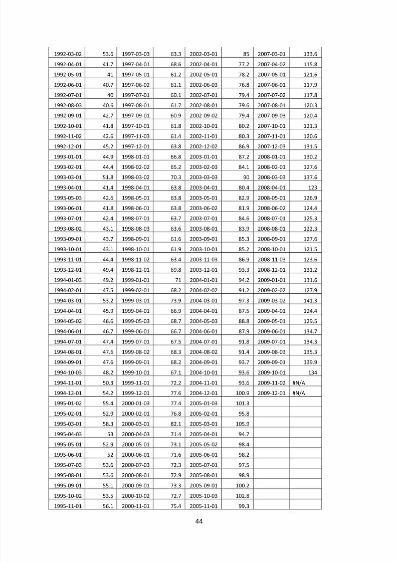
8/6/2019 Long Term and Shrt Run relationship between Macroeconomic variables and stock market in India
http://slidepdf.com/reader/full/long-term-and-shrt-run-relationship-between-macroeconomic-variables-and-stock 44/48
44
1992-03-02 53.6 1997-03-03 63.3 2002-03-01 85 2007-03-01 133.6
1992-04-01 41.7 1997-04-01 68.6 2002-04-01 77.2 2007-04-02 115.8
1992-05-01 41 1997-05-01 61.2 2002-05-01 78.2 2007-05-01 121.6
1992-06-01 40.7 1997-06-02 61.1 2002-06-03 76.8 2007-06-01 117.9
1992-07-01 40 1997-07-01 60.1 2002-07-01 79.4 2007-07-02 117.8
1992-08-03 40.6 1997-08-01 61.7 2002-08-01 79.6 2007-08-01 120.3
1992-09-01 42.7 1997-09-01 60.9 2002-09-02 79.4 2007-09-03 120.4
1992-10-01 41.8 1997-10-01 61.8 2002-10-01 80.2 2007-10-01 121.3
1992-11-02 42.6 1997-11-03 61.4 2002-11-01 80.3 2007-11-01 120.6
1992-12-01 45.2 1997-12-01 63.8 2002-12-02 86.9 2007-12-03 131.5
1993-01-01 44.9 1998-01-01 66.8 2003-01-01 87.2 2008-01-01 130.2
1993-02-01 44.4 1998-02-02 65.2 2003-02-03 84.1 2008-02-01 127.6
1993-03-01 51.8 1998-03-02 70.3 2003-03-03 90 2008-03-03 137.6
1993-04-01 41.4 1998-04-01 63.8 2003-04-01 80.4 2008-04-01 123
1993-05-03 42.6 1998-05-01 63.8 2003-05-01 82.9 2008-05-01 126.9
1993-06-01 41.8 1998-06-01 63.8 2003-06-02 81.9 2008-06-02 124.4
1993-07-01 42.4 1998-07-01 63.7 2003-07-01 84.6 2008-07-01 125.3
1993-08-02 43.1 1998-08-03 63.6 2003-08-01 83.9 2008-08-01 122.3
1993-09-01 43.7 1998-09-01 61.6 2003-09-01 85.3 2008-09-01 127.6
1993-10-01 43.1 1998-10-01 61.9 2003-10-01 85.2 2008-10-01 121.5
1993-11-01 44.4 1998-11-02 63.4 2003-11-03 86.9 2008-11-03 123.6
1993-12-01 49.4 1998-12-01 69.8 2003-12-01 93.3 2008-12-01 131.2
1994-01-03 49.2 1999-01-01 71 2004-01-01 94.2 2009-01-01 131.6
1994-02-01 47.5 1999-02-01 68.2 2004-02-02 91.2 2009-02-02 127.9
1994-03-01 53.2 1999-03-01 73.9 2004-03-01 97.3 2009-03-02 141.3
1994-04-01 45.9 1999-04-01 66.9 2004-04-01 87.5 2009-04-01 124.4
1994-05-02 46.6 1999-05-03 68.7 2004-05-03 88.8 2009-05-01 129.5
1994-06-01 46.7 1999-06-01 66.7 2004-06-01 87.9 2009-06-01 134.7
1994-07-01 47.4 1999-07-01 67.5 2004-07-01 91.8 2009-07-01 134.3
1994-08-01 47.6 1999-08-02 68.3 2004-08-02 91.4 2009-08-03 135.3
1994-09-01 47.6 1999-09-01 68.2 2004-09-01 93.7 2009-09-01 139.9
1994-10-03 48.2 1999-10-01 67.1 2004-10-01 93.6 2009-10-01 134
1994-11-01 50.3 1999-11-01 72.2 2004-11-01 93.6 2009-11-02 #N/A
1994-12-01 54.2 1999-12-01 77.6 2004-12-01 100.9 2009-12-01 #N/A1995-01-02 55.4 2000-01-03 77.4 2005-01-03 101.3
1995-02-01 52.9 2000-02-01 76.8 2005-02-01 95.8
1995-03-01 58.3 2000-03-01 82.1 2005-03-01 105.9
1995-04-03 53 2000-04-03 71.4 2005-04-01 94.7
1995-05-01 52.9 2000-05-01 73.1 2005-05-02 98.4
1995-06-01 52 2000-06-01 71.6 2005-06-01 98.2
1995-07-03 53.6 2000-07-03 72.3 2005-07-01 97.5
1995-08-01 53.6 2000-08-01 72.9 2005-08-01 98.9
1995-09-01 55.1 2000-09-01 73.3 2005-09-01 100.2
1995-10-02 53.5 2000-10-02 72.7 2005-10-03 102.8
1995-11-01 56.1 2000-11-01 75.4 2005-11-01 99.3
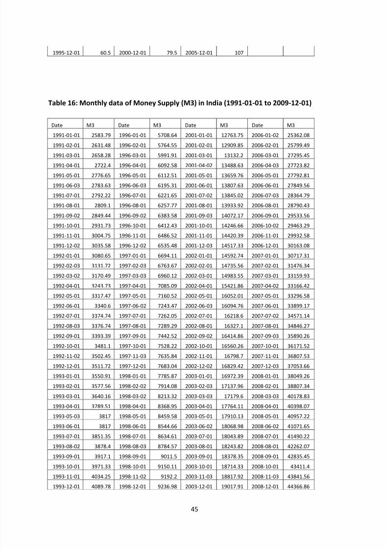
8/6/2019 Long Term and Shrt Run relationship between Macroeconomic variables and stock market in India
http://slidepdf.com/reader/full/long-term-and-shrt-run-relationship-between-macroeconomic-variables-and-stock 45/48
45
1995-12-01 60.5 2000-12-01 79.5 2005-12-01 107
Table 16: Monthly data of Money Supply (M3) in India (1991-01-01 to 2009-12-01)
Date M3 Date M3 Date M3 Date M3
1991-01-01 2583.79 1996-01-01 5708.64 2001-01-01 12763.75 2006-01-02 25362.08
1991-02-01 2631.48 1996-02-01 5764.55 2001-02-01 12909.85 2006-02-01 25799.49
1991-03-01 2658.28 1996-03-01 5991.91 2001-03-01 13132.2 2006-03-01 27295.45
1991-04-01 2722.4 1996-04-01 6092.58 2001-04-02 13488.63 2006-04-03 27723.82
1991-05-01 2776.65 1996-05-01 6112.51 2001-05-01 13659.76 2006-05-01 27792.81
1991-06-03 2783.63 1996-06-03 6195.31 2001-06-01 13807.63 2006-06-01 27849.56
1991-07-01 2792.22 1996-07-01 6221.65 2001-07-02 13845.02 2006-07-03 28364.79
1991-08-01 2809.1 1996-08-01 6257.77 2001-08-01 13933.92 2006-08-01 28790.43
1991-09-02 2849.44 1996-09-02 6383.58 2001-09-03 14072.17 2006-09-01 29533.56
1991-10-01 2931.73 1996-10-01 6412.43 2001-10-01 14246.66 2006-10-02 29463.29
1991-11-01 3004.75 1996-11-01 6486.52 2001-11-01 14420.39 2006-11-01 29932.58
1991-12-02 3035.58 1996-12-02 6535.48 2001-12-03 14517.33 2006-12-01 30163.08
1992-01-01 3080.65 1997-01-01 6694.11 2002-01-01 14592.74 2007-01-01 30717.31
1992-02-03 3131.72 1997-02-03 6763.67 2002-02-01 14735.56 2007-02-01 31476.34
1992-03-02 3170.49 1997-03-03 6960.12 2002-03-01 14983.55 2007-03-01 33159.93
1992-04-01 3243.73 1997-04-01 7085.09 2002-04-01 15421.86 2007-04-02 33166.421992-05-01 3317.47 1997-05-01 7160.52 2002-05-01 16052.01 2007-05-01 33296.58
1992-06-01 3340.6 1997-06-02 7243.47 2002-06-03 16094.76 2007-06-01 33899.17
1992-07-01 3374.74 1997-07-01 7262.05 2002-07-01 16218.6 2007-07-02 34571.14
1992-08-03 3376.74 1997-08-01 7289.29 2002-08-01 16327.1 2007-08-01 34846.27
1992-09-01 3393.39 1997-09-01 7442.52 2002-09-02 16414.86 2007-09-03 35890.26
1992-10-01 3481.1 1997-10-01 7528.22 2002-10-01 16560.26 2007-10-01 36171.52
1992-11-02 3502.45 1997-11-03 7635.84 2002-11-01 16798.7 2007-11-01 36807.53
1992-12-01 3511.72 1997-12-01 7683.04 2002-12-02 16829.42 2007-12-03 37053.66
1993-01-01 3550.91 1998-01-01 7785.87 2003-01-01 16972.39 2008-01-01 38049.26
1993-02-01 3577.56 1998-02-02 7914.08 2003-02-03 17137.96 2008-02-01 38807.34
1993-03-01 3640.16 1998-03-02 8213.32 2003-03-03 17179.6 2008-03-03 40178.83
1993-04-01 3789.51 1998-04-01 8368.95 2003-04-01 17764.11 2008-04-01 40398.07
1993-05-03 3817 1998-05-01 8459.58 2003-05-01 17910.13 2008-05-01 40957.22
1993-06-01 3817 1998-06-01 8544.66 2003-06-02 18068.98 2008-06-02 41071.65
1993-07-01 3851.35 1998-07-01 8634.61 2003-07-01 18043.89 2008-07-01 41490.22
1993-08-02 3878.4 1998-08-03 8784.57 2003-08-01 18243.82 2008-08-01 42262.07
1993-09-01 3917.1 1998-09-01 9011.5 2003-09-01 18378.35 2008-09-01 42835.45
1993-10-01 3971.33 1998-10-01 9150.11 2003-10-01 18714.33 2008-10-01 43411.4
1993-11-01 4034.25 1998-11-02 9192.2 2003-11-03 18817.92 2008-11-03 43841.56
1993-12-01 4089.78 1998-12-01 9236.98 2003-12-01 19017.91 2008-12-01 44366.86
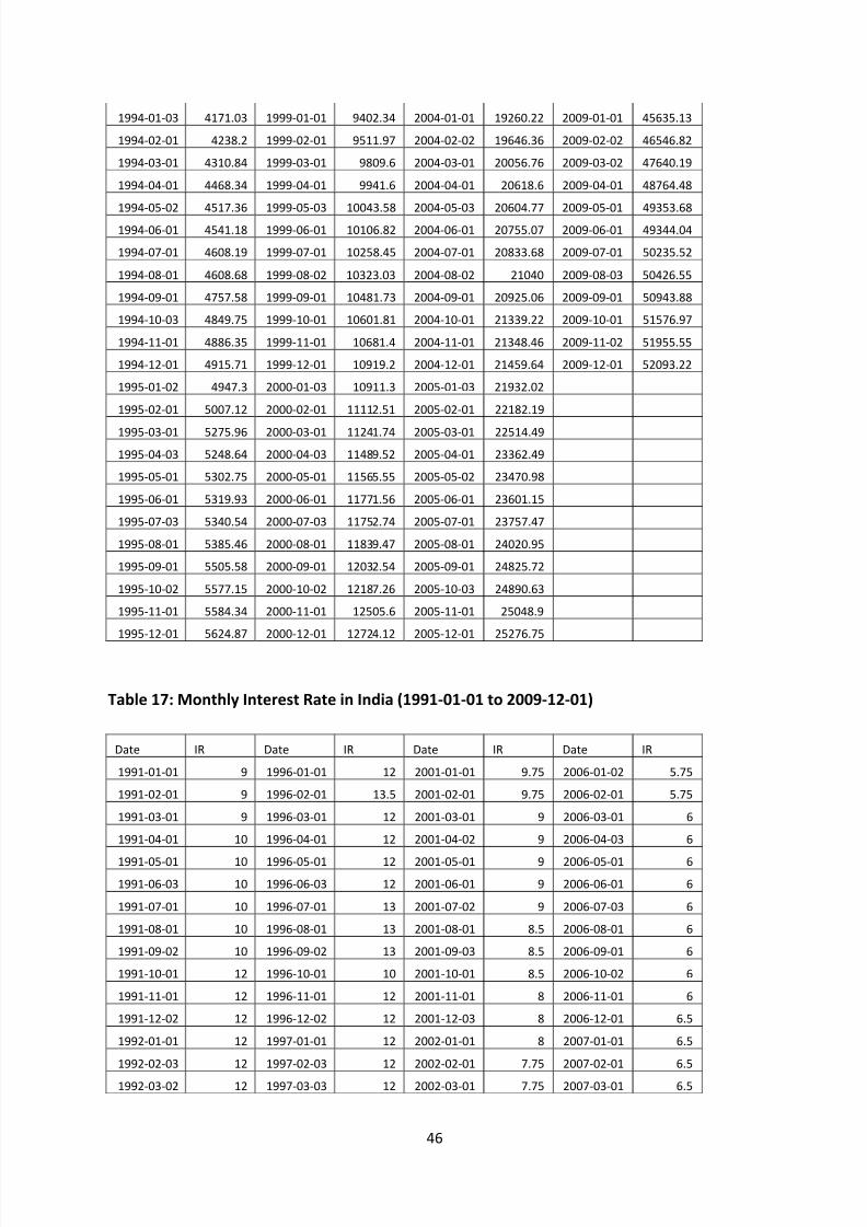
8/6/2019 Long Term and Shrt Run relationship between Macroeconomic variables and stock market in India
http://slidepdf.com/reader/full/long-term-and-shrt-run-relationship-between-macroeconomic-variables-and-stock 46/48
46
1994-01-03 4171.03 1999-01-01 9402.34 2004-01-01 19260.22 2009-01-01 45635.13
1994-02-01 4238.2 1999-02-01 9511.97 2004-02-02 19646.36 2009-02-02 46546.82
1994-03-01 4310.84 1999-03-01 9809.6 2004-03-01 20056.76 2009-03-02 47640.19
1994-04-01 4468.34 1999-04-01 9941.6 2004-04-01 20618.6 2009-04-01 48764.48
1994-05-02 4517.36 1999-05-03 10043.58 2004-05-03 20604.77 2009-05-01 49353.68
1994-06-01 4541.18 1999-06-01 10106.82 2004-06-01 20755.07 2009-06-01 49344.04
1994-07-01 4608.19 1999-07-01 10258.45 2004-07-01 20833.68 2009-07-01 50235.52
1994-08-01 4608.68 1999-08-02 10323.03 2004-08-02 21040 2009-08-03 50426.55
1994-09-01 4757.58 1999-09-01 10481.73 2004-09-01 20925.06 2009-09-01 50943.88
1994-10-03 4849.75 1999-10-01 10601.81 2004-10-01 21339.22 2009-10-01 51576.97
1994-11-01 4886.35 1999-11-01 10681.4 2004-11-01 21348.46 2009-11-02 51955.55
1994-12-01 4915.71 1999-12-01 10919.2 2004-12-01 21459.64 2009-12-01 52093.22
1995-01-02 4947.3 2000-01-03 10911.3 2005-01-03 21932.02
1995-02-01 5007.12 2000-02-01 11112.51 2005-02-01 22182.19
1995-03-01 5275.96 2000-03-01 11241.74 2005-03-01 22514.49
1995-04-03 5248.64 2000-04-03 11489.52 2005-04-01 23362.49
1995-05-01 5302.75 2000-05-01 11565.55 2005-05-02 23470.98
1995-06-01 5319.93 2000-06-01 11771.56 2005-06-01 23601.15
1995-07-03 5340.54 2000-07-03 11752.74 2005-07-01 23757.47
1995-08-01 5385.46 2000-08-01 11839.47 2005-08-01 24020.95
1995-09-01 5505.58 2000-09-01 12032.54 2005-09-01 24825.72
1995-10-02 5577.15 2000-10-02 12187.26 2005-10-03 24890.63
1995-11-01 5584.34 2000-11-01 12505.6 2005-11-01 25048.9
1995-12-01 5624.87 2000-12-01 12724.12 2005-12-01 25276.75
Table 17: Monthly Interest Rate in India (1991-01-01 to 2009-12-01)
Date IR Date IR Date IR Date IR
1991-01-01 9 1996-01-01 12 2001-01-01 9.75 2006-01-02 5.75
1991-02-01 9 1996-02-01 13.5 2001-02-01 9.75 2006-02-01 5.75
1991-03-01 9 1996-03-01 12 2001-03-01 9 2006-03-01 6
1991-04-01 10 1996-04-01 12 2001-04-02 9 2006-04-03 6
1991-05-01 10 1996-05-01 12 2001-05-01 9 2006-05-01 6
1991-06-03 10 1996-06-03 12 2001-06-01 9 2006-06-01 6
1991-07-01 10 1996-07-01 13 2001-07-02 9 2006-07-03 6
1991-08-01 10 1996-08-01 13 2001-08-01 8.5 2006-08-01 6
1991-09-02 10 1996-09-02 13 2001-09-03 8.5 2006-09-01 6
1991-10-01 12 1996-10-01 10 2001-10-01 8.5 2006-10-02 6
1991-11-01 12 1996-11-01 12 2001-11-01 8 2006-11-01 6
1991-12-02 12 1996-12-02 12 2001-12-03 8 2006-12-01 6.5
1992-01-01 12 1997-01-01 12 2002-01-01 8 2007-01-01 6.5
1992-02-03 12 1997-02-03 12 2002-02-01 7.75 2007-02-01 6.5
1992-03-02 12 1997-03-03 12 2002-03-01 7.75 2007-03-01 6.5
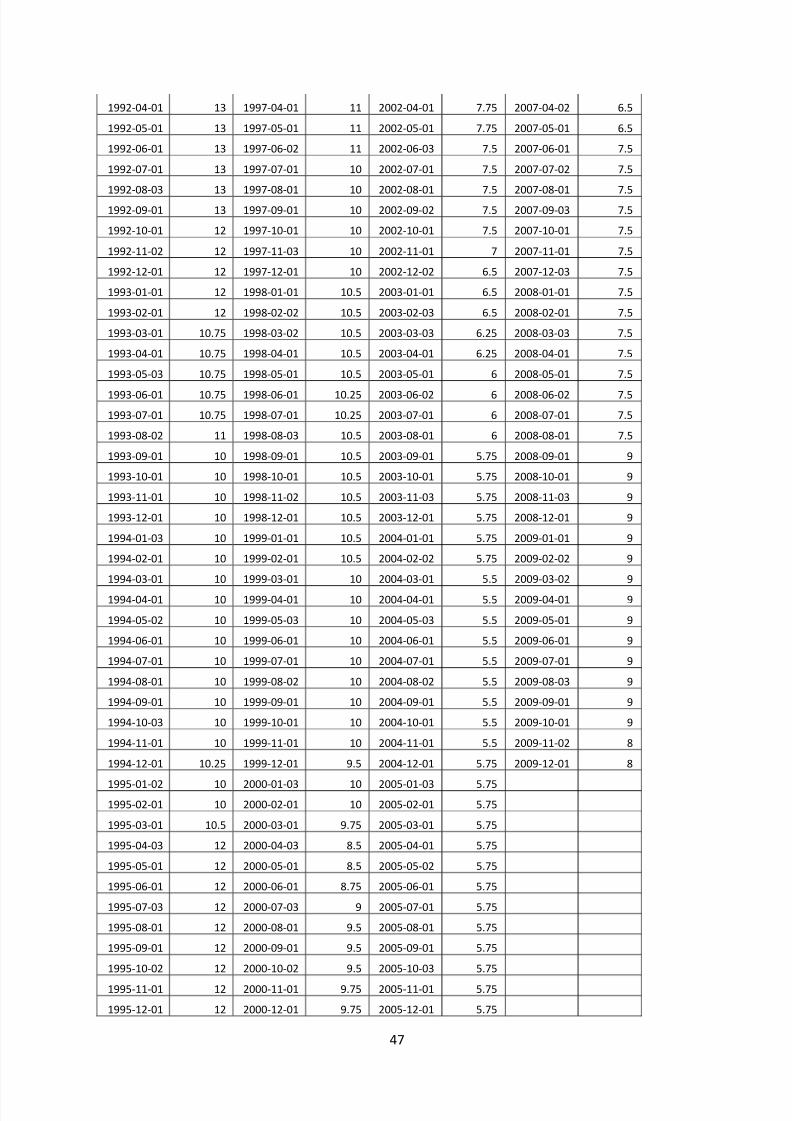
8/6/2019 Long Term and Shrt Run relationship between Macroeconomic variables and stock market in India
http://slidepdf.com/reader/full/long-term-and-shrt-run-relationship-between-macroeconomic-variables-and-stock 47/48
47
1992-04-01 13 1997-04-01 11 2002-04-01 7.75 2007-04-02 6.5
1992-05-01 13 1997-05-01 11 2002-05-01 7.75 2007-05-01 6.5
1992-06-01 13 1997-06-02 11 2002-06-03 7.5 2007-06-01 7.5
1992-07-01 13 1997-07-01 10 2002-07-01 7.5 2007-07-02 7.5
1992-08-03 13 1997-08-01 10 2002-08-01 7.5 2007-08-01 7.5
1992-09-01 13 1997-09-01 10 2002-09-02 7.5 2007-09-03 7.5
1992-10-01 12 1997-10-01 10 2002-10-01 7.5 2007-10-01 7.5
1992-11-02 12 1997-11-03 10 2002-11-01 7 2007-11-01 7.5
1992-12-01 12 1997-12-01 10 2002-12-02 6.5 2007-12-03 7.5
1993-01-01 12 1998-01-01 10.5 2003-01-01 6.5 2008-01-01 7.5
1993-02-01 12 1998-02-02 10.5 2003-02-03 6.5 2008-02-01 7.5
1993-03-01 10.75 1998-03-02 10.5 2003-03-03 6.25 2008-03-03 7.5
1993-04-01 10.75 1998-04-01 10.5 2003-04-01 6.25 2008-04-01 7.5
1993-05-03 10.75 1998-05-01 10.5 2003-05-01 6 2008-05-01 7.5
1993-06-01 10.75 1998-06-01 10.25 2003-06-02 6 2008-06-02 7.5
1993-07-01 10.75 1998-07-01 10.25 2003-07-01 6 2008-07-01 7.5
1993-08-02 11 1998-08-03 10.5 2003-08-01 6 2008-08-01 7.5
1993-09-01 10 1998-09-01 10.5 2003-09-01 5.75 2008-09-01 9
1993-10-01 10 1998-10-01 10.5 2003-10-01 5.75 2008-10-01 9
1993-11-01 10 1998-11-02 10.5 2003-11-03 5.75 2008-11-03 9
1993-12-01 10 1998-12-01 10.5 2003-12-01 5.75 2008-12-01 9
1994-01-03 10 1999-01-01 10.5 2004-01-01 5.75 2009-01-01 9
1994-02-01 10 1999-02-01 10.5 2004-02-02 5.75 2009-02-02 9
1994-03-01 10 1999-03-01 10 2004-03-01 5.5 2009-03-02 9
1994-04-01 10 1999-04-01 10 2004-04-01 5.5 2009-04-01 9
1994-05-02 10 1999-05-03 10 2004-05-03 5.5 2009-05-01 9
1994-06-01 10 1999-06-01 10 2004-06-01 5.5 2009-06-01 9
1994-07-01 10 1999-07-01 10 2004-07-01 5.5 2009-07-01 9
1994-08-01 10 1999-08-02 10 2004-08-02 5.5 2009-08-03 9
1994-09-01 10 1999-09-01 10 2004-09-01 5.5 2009-09-01 9
1994-10-03 10 1999-10-01 10 2004-10-01 5.5 2009-10-01 9
1994-11-01 10 1999-11-01 10 2004-11-01 5.5 2009-11-02 8
1994-12-01 10.25 1999-12-01 9.5 2004-12-01 5.75 2009-12-01 8
1995-01-02 10 2000-01-03 10 2005-01-03 5.751995-02-01 10 2000-02-01 10 2005-02-01 5.75
1995-03-01 10.5 2000-03-01 9.75 2005-03-01 5.75
1995-04-03 12 2000-04-03 8.5 2005-04-01 5.75
1995-05-01 12 2000-05-01 8.5 2005-05-02 5.75
1995-06-01 12 2000-06-01 8.75 2005-06-01 5.75
1995-07-03 12 2000-07-03 9 2005-07-01 5.75
1995-08-01 12 2000-08-01 9.5 2005-08-01 5.75
1995-09-01 12 2000-09-01 9.5 2005-09-01 5.75
1995-10-02 12 2000-10-02 9.5 2005-10-03 5.75
1995-11-01 12 2000-11-01 9.75 2005-11-01 5.75
1995-12-01 12 2000-12-01 9.75 2005-12-01 5.75

8/6/2019 Long Term and Shrt Run relationship between Macroeconomic variables and stock market in India
http://slidepdf.com/reader/full/long-term-and-shrt-run-relationship-between-macroeconomic-variables-and-stock 48/48