THE RELATIONSHIP BETWEEN MACROECONOMICVARIABLES AND THE CHINESE STOCK MARKET-AN

APPLICATION OF VECTOR ERROR CORRECTIONMODEL

Submitted by

Zhe Zeng

A thesis submitted to the Department of Statistics inpartial fulfillment of the requirements for a two-year Master

degree in Statistics in the Faculty of Social Sciences

Supervisor

Per Johansson

Spring, 2017

ABSTRACT

Using Johansen’s vector error correction model, this paper investigates the long-term equi-

librium between stock price and six selected macroeconomic variables in China. On testing dif-

ferent VECM models, we find that there is no long-term equilibrium between stock price and

6 macroeconomic variables, although there may exist long-term equilibrium among macroe-

conomic variables themselves. However, by applying impulse responses plots, we find that

industrial production, exchange rate and interest rate do have effects on stock price that are

consistent with economic hypotheses. This indicates that Chinese stock market does reflect

economic situation to some extent, so it can be considered as an indicator of the real economy.

Contents

1 Introduction and review of literature 3

2 Hypothesized Equilibrium Relations 5

3 Methodology 6

4 Data 8

5 Empirical Analysis 10

5.1 Checking Stationarity . . . . . . . . . . . . . . . . . . . . . . . . . . . . . . . 10

5.2 Model Specification . . . . . . . . . . . . . . . . . . . . . . . . . . . . . . . . 13

5.3 Cointegration Test . . . . . . . . . . . . . . . . . . . . . . . . . . . . . . . . . 15

5.4 VECM Based On VAR(2) . . . . . . . . . . . . . . . . . . . . . . . . . . . . . 17

5.5 Impulse Responses and Variance Decomposition . . . . . . . . . . . . . . . . 18

6 Conclusion 20

2

1 Introduction and review of literature

Some people think stock market is the barometer of the real economy, maybe this opinion

is true in some mature markets such as the U.S., Japan, and Sweden. However, this seems not

the case for Chinese stock market.

During 1992, stock market drop to 400 points from 1500 points. However, the real econ-

omy was working well at that time. Before which, former state leader Mr. Deng just finished

his famous 1992 "southern tour" and the whole country was concentrating on developing. Al-

though the market soon bottom out, it’s nothing to do with the real economy, but the result of

the government’s bailout program.

In 1999, China had yet recovered from The Asian financial crisis. However, a bull market1

emerged, the stock price first rise from 1050 points to 1700 points, then drop slightly, finally

peaked at 2245 points begging next year.

After that, the stock market drop to 998 points after years of decline until 2005. Then

another bull market emerged. This time, it is related with the real economy. Several reasons

result in this bull market. First reason is the rise of RMB exchange rate from, which led a inflow

of foreign currency, and then a increase in currency liquidity2 and stock price. Second reason is

the reform of the shareholder structure in listed companies and this resolved this longstanding

institutional problem that hindered the development of the securities market. The third reason

is home prices in the whole country was rising at that time, which induced the the development

of other industries like steel, cement, furniture, etc. The result is the stock market rose to

unbelievable 6124 points on the rampage, this is the only bull market that is close correlated

with the real economic situation.

In October 2014, the bull market that rose from 1800 points to 5100 points is still unrelated

with real economy, many industries are falling down with no profit or very little profit at that

time. Many people just entered the stock market for speculation, some even rushed into the

market with up to 5 times leverage.

Taken together, the stock market seems a reflection of current economic situation some-

times, but other times, it’s totally unrelated with the real economy. Some people argued that

the reason behind this phenomenon are the RMB is not freely convertible, many channels to

invest in China, and Share splitting, etc. Stock market is really not the barometer of the real

1A market in which stock prices are rising, encouraging buying.2Monetary circulation quantity in the market.

3

economy in China? Are macroeconomic variables really not correlated with stock price? This

is what this article want to examine.

As early as 1930s, Fisher (1930) has begin his theoretical research on stock-focused asset

prices fluctuation, which try to reveal the underlying mechanism that how macroeconomic

variables affect stock price. After that, a lot of scholars had conducted deep research on this

topic. Until recently, the most frequently used model in this regard is Arbitrage Pricing Theory

developed by Ross (1976), which essentially measure the risk premium attach to risk factors

and test if they are priced into stock returns. Using this model, Chen Roll and Rose (1986)

showed that economic indicators do have significant effects on stock returns.

The development of cointegration analysis provide researcher another choice of study this

relationship. Granger(1986) verified the long-run equilibrium between the economic indica-

tors and stock prices found by Chen Roll and Rose (1986) through a cointegration analysis.

In statistics, several time-series variables are cointegrated if they are nonstationary variables

and the a linear combination of them are stationary. In economics, such a linear combination

implies a long-run equilibrium among variables.

Compared to standard vector autoregressive model, one advantage of cointegration analysis

is that it provide a better framework for examining both the long-run relationships and the

short-run adjustments through building an error correction model, which provide us a better

interpretation of model. In this paper, we employ Johansen’s (1991) vector error correction

model to check if there exist any long-run equilibrium between macroeconomic variables and

stock price in China.

Many researchers have examine the relationship of the macroeconomic variables and the

stock price in other market using vector error correction model. Mukherjee and Naka (1995)

concluded Tokyo stock exchange index does have a long-term relationship with the macroeco-

nomic variables, namely the industrial production, money supply, inflation, long-term govern-

ment bond, call money rate and exchange rate. The sign of the long-term elasticity coefficients

are generally consistent with their hypothesized equilibrium relations.

Maysami and Koh (2000) verified the relationship using data collected from Singapore.

They found that although industrial production and trade are are not cointegrated with stock

price, money supply growth, inflation, changes in short-term and long-term interest rate and

changes in exchange rate do have a long-run equilibrium with the changes in Singapore’s stock

market levels. They also show that Singapore stock market are cointegrated with the U.S. and

4

Japanese market

Some research have also been conducted in Chinese stock market, Liu and Shrestha (2008)

show that the cointegrated relationship does exist between the macroeconomic variables and

stock price in the highly speculative Chinese stock market.

This paper will try to construct the VECM model with more recently data and incorporate

impulse responses and variance decomposition to better investigate the relationship between

stock price and macroeconomic indicators.

2 Hypothesized Equilibrium Relations

Firstly, we need to establish a basic hypothesis between the Chinese stock price and the

macroeconomic variables: money supply M2, inflation, industrial production, RMB currency

exchange, short-term interest rate and long-term interest rate base on "simple and intuitive

financial theory" as Chen, Roll and Ross (1986) suggested.

The relationship between the money supply and the stock price is not very clear. The

increase of money supply will stimulate the economy by giving tremendous liquidity to the

market, which tend to increase future cash flow and result in an increase of stock price. How-

ever, an increase in money supply is considered to be accompanied by an increase of inflation,

which leads to an increase in discount rate, so this implies a negative effect between the money

supply and stock price. So the effect of stock price on stock price is still an empirical question.

The relationship between the interest rate and stock price is pretty clear, and increase in

the interest rate will increase the attraction of the interest-bearing securities and decrease the

attraction of stock, people will also prefer putting money in banks if the interest increase.

Additionally, an increase in both long-run and short-run interest rate will tend to increase the

risk-free interest rate, so does the discount rate. To sum up, we assume that there exist an

negative relationship between the interest rate and the stock price.

The effect of inflation rate on stock price is pretty straightforward, we hypothesize a neg-

ative relationship between them. An expected inflation rate will tend lower the stock price by

leading a tightening economic policies. Moreover, an increase in inflation rate will raise in

discount rate by raising the risk-free interest rate. This hypothesized relationship have been

verified by many empirical studies, such as Fama and Schwert (1977), Geske and Roll (1983),

and Chen, Roll and Ross (1986).

5

We hypothesize industrial production has an positive effect on stock price, this one is also

very straightforward. The prosperity of the industrial production will lead a development of

whole economy, so there will be an increase in expected in future cash flow, so do the stock

prices. This relationship is particularly important in for china, for which, as the world factory,

industrial production is literally the pillar of the economy.

The effect of RMB exchange rate on Chinese stock price is also an empirical question. On

one hand, an appreciation of RMB will lead to a relative increase of price of Chinese products

in foreign markets, so a decrease of competitiveness and demand of Chinese products, so the

earning for Chinese company will drop. On the other hand, an an appreciation of RMB will

attract an inflow of foreign currency, this will stimulate the whole economy, and is likely to

drive the stock prices going up.

3 Methodology

We’ll check if there exist any long-term relationship between macroeconomic variables and

stock price using Johansen’s VECM. Although Engle-Granger’s two-step procedure can also be

used to get the long-run relationship in a multivariate context, we prefer to the use Johansen’s

procedure, which use maximum likelihood estimation to build cointegrated variables while

Engle-Granger’s two-step procedure use OLS estimation. The advantage of Johansen’s proce-

dure over Engle-Granger’s two-step procedure is that it could find more than one cointegration

relations and more efficient estimators. The vector error correction takes the following form:

∆Yt =k−1∑j=1

Γj∆Yt−j + ΠYt−1 + φDt + εt (1)

where∑k−1

j=0 Γj∆Yt−j represent the vector autoregressive component (VAR). ΠYt−1 is the error-

correction component. φDt is the deterministic term including constant term and time trend. εt

is the white noise error term, εt is i.i.d. ∼ Nn(0,Ω). If data vector Yt is no more than I(1)3 and

could be cointegrated, Π has a reduced rank r < n and be decomposed as Π = αβ′. α is called

short-run adjustment, β is the combining matrix of r long-run cointegrating vectors. A large

α implies a faster convergence to long-term equilibrium when there is a short-term deviation

from this long-term equilibrium.

3Integration of order 1.

6

In Johansen’s VECM procedure, the basic assumption is the data vector Yt is no more than

I(1), specically, if Yt = (Y1t, ..., Ynt)′, then either Yit ∼ I(0) or ∆Yit ∼ I(0). So we’ll need

to check if the variables in levels and their first difference is stationary. To do this, we use the

augmented Dickey-Fuller test (ADF) and Phillips-perron test (PP) to check the unit roots. Then

we can examine if there is any cointegrated relation between variables of integrated of order 1.

Vector error correction model is nothing more than an vector autoregressive model, so nest

step is to decide the lag length of the the model. To do this, we use four information criteria,

namely Akaike information criterion (AIC), Hannan-Quinn criterion (HQ), Schwarz criterion

(SC) and Akaike’s final prediction error criterion (FPE). AIC = 2k − 2ln(Lmax), HQ =

−2Lmax + 2kln(ln(n)) and SC = −2Lmax + mlnn. These information criteria minimize the

logarithm of residual sum of square adjusted for sample size and number of parameters, and

then the lag length is corresponding to the statistics with minimized value.

The nest step is to estimate the vector error correction model, and then determine the rank

of Π = αβ′. The eigenvector in β′ are estimated from the canonical correlation of the set of

residuals from the regression equations. Then we could determine the order of cointegration

r by calculate the full rank of Π. In order to determine the rank of Π, we use the maximum

eigenvalue test λmax and the trace test λtrace, where

λmax = −T ln(1− λr+1), (2)

λtrace = −Tp∑

i=r+1

ln(1− λi), (3)

the λi are the estimated eigenvalues. We will reject the hypothesis that there are cointegrating

relationships if the rank of Π is 0, and r = n implies that Π is full rank, hence there is no unit

root and thus the system is I(0), there is no need to use VECM, VAR is enough.

After determining the order of cointegration, we could estimate the VECM and get the long-

run cointegrating vectors and the short-run adjustment. Usually, the rank of Π is more than 1,

so there will be more than one cointegrating relationships. In that case, we tend to use the the

eigenvector corresponding to the largest eigenvalue according to Mukherjee and Naka (1995)

and Maysami and Koh (2000). Because we want to examine the effect of macroeconomic

variables on stock price, so we will normalize the β′ with respect to the coefficient for stock

price.

Then we need to test if the the long-run parameters β′ are significant, in order to do this, we

7

take use of likelihood ratio test. Hypotheses on the long-run coefficients β′ can be formulated

in terms of linear restrictions on β′:

H0 : R′β = 0 or β = BΨ, (4)

where Ψ are the unknown parameters in the cointegrating vectors β, B = R⊥ and R⊥ is the

orthogonal complement of R such that R′R⊥ = 0. The LR test statistic is:

−2logQ(H0|H(r)) = T

r∑i=1

log((1− λ∗i )/(1− λi)), (5)

The LR test statistic is asymptotically χ2 distributed with degrees of freedom. In order to test

whether single coefficient of β is significant, we could set one element of R equals to 1 while

others are 0.

Finally, our interest lies in the impulse responses and variance decomposition, which help

explain how shocks transmit in the system and how much of the variance of the forecast error

of yi,t+s is due to an exogenous shock to yj,t respectively. For multivariate case, the impulse

responses variable i at time t+ s of a shock to variable j at time t is defined as:

∂yi,t+s

∂εj,t, (6)

and the proportion of forecast error variance of variable m attributable to variable j at horizon s

is:

Ξj,s(m,m)

Ξs(m,m), (7)

The numerator is the contribution of variable j to MSE while the denominator is the variables’

total MSE.

4 Data

The stock price and six macroeconomic variables data and their explanation are presented in

upper panel of Table 1. The seven variables including the stock price are all monthly data col-

lected from http://d.qianzhan.com/, which is an online database contain a variety of economic

8

Variables Definitions of variables

LshindextNatural logarithm of the month-end Shanghai StockExchange Composite Index

LM2tNatural logarithm of the month-end M2 money supplyin China

LCPItNatural logarithm of the month-end Consumer PriceIndex

LPMItNatural logarithm of the month-end PurchasingManagers’ Index

LRMBindextNatural logarithm of the month-end Real effectiveexchange rate index for RMB

LinttNatural logarithm of the month-end 14-day ShanghaiInterbank Offered Rate (Shibor)

LY 5BtNatural logarithm of the month-end yield on 5-yeargovernment securities

Transformation Definitions of transformation

∆shindext = Lshindext − Lshindext−1Monthly return on the Shanghai Stock Exchange(ex-dividend)

∆M2t = LM2t − LM2t−1 Monthly growth rate of money supply∆CPIt = LCPIt − LCPIt−1 Monthly realized inflation rate∆PMIt = LPMIt − LPMIt−1 Monthly change of PMI∆RMBindext = LRMBindext − LRMBindext−1 Monthly change of RMB exchange rate∆intt = Lintt − Lintt−1 Monthly return of 14-day Shibor∆Y 5Bt = LY 5Bt − LY 5Bt−1 Monthly return of 5-year government securities

Table 1: Definitions of variables and their first differences

data of China. There are several remarkable points:

1. The stock price is represented by the price index instead of price itself, and SSE Com-

posite Index is calculated using a Paasche weighted composite price index formula.

2. The Purchasing Managers’ Index (PMI) is an indicator of the economic health of the

manufacturing sector, this is a suitable variable for industrial production.

3. We use exchange rate index instead of any bilateral exchange rate here since exchange

rate index weights together different bilateral exchange rates to create an effective ex-

change rate which better represent the value of a country’s currency.

4. Here we use Shibor instead of benchmark bank loan rate since benchmark bank loan rate

is determined by the central bank which means it’s not floating with the market.

Since these variable are all variables related to economy and finance, so are interested in how

the percentage change in the stock price is related with the percentage change in the macroeco-

nomic variables. In this situation, we take natural logarithm the variables and use them in the

model. Because we will also need to check the stationary of the first differences of variables,

so their explanation are also presented in Table 1.

9

The the data period are from July 2009 to Feb February 2017, totally 92 observations. The

reason this period of time is chosen is because subprime crisis happened in the United States

in 2007 which in turn, led to global financial tsunami. This global financial crisis unavoidably

impacted China which is a member of global financial and trade system. From October 2007

to October 2008, Chinese stock market dropped from 6124 points to 1664 points, biggest fall

reached 73%. So we are interested in the performance of stock market in the post-crisis era.

Also, some data are only available since 2009, so this period of time is when we can get the

complete data of all the variables we use in this paper.

5 Empirical Analysis

5.1 Checking Stationarity

In order to use Johansen’s VECM procedure, we’ll need to check if the variables and their

first difference are stationary. Table 2 gives us the summary statistics of the variables in levels

and in first differences. After the first order difference, standard deviation decline significantly,

Median Mean Std Dev Minimum Maxium skew kurtosisVariables in levels

Lshindext 7.90 7.89 0.20 7.59 8.44 0.41 -0.34LM2t 13.85 13.81 0.30 13.26 14.27 -0.21 -1.19LCPIt 4.71 4.69 0.06 4.57 4.78 -0.59 -0.79LPMIt 3.94 3.95 0.05 3.87 4.08 1.09 0.55LRMBindext 4.74 4.73 0.10 4.56 4.88 -0.01 -1.34Lintt 1.22 1.18 0.36 0.39 1.96 -0.33 -0.29LY 5Bt 1.17 1.17 0.15 0.91 1.49 0.26 -0.81

Variables in first differences∆shindext 0.01 0.00 0.07 -0.26 0.19 -0.60 1.93∆M2t 0.01 0.01 0.01 -0.01 0.04 0.21 -0.09∆CPIt 0.00 0.00 0.01 -0.01 0.02 0.37 -0.20∆PMIt 0.00 0.00 0.03 -0.07 0.06 -0.12 -0.13∆RMBindext 0.00 0.00 0.01 -0.03 0.04 0.23 -0.02∆intt 0.01 0.01 0.21 -0.51 0.70 0.50 1.72∆Y 5Bt 0.00 0.00 0.05 -0.09 0.18 0.71 1.83

Table 2: Descriptive statistics of variables

and all the variables seems concentrate on the neighbor of 0, this is a good sign of integration

of 1.

This guess is verified in Figure 1 and Figure 2 which show the time series plot for variables

in levels and in first differences. In Figure 1, it seems none of variables in levels are stationary,

moreover, some of them are likely to have trends. For Lshindext, it keeps declining from the

beginning of the data until early 2014, then rebound rapidly at the latter half of this year which

10

Figure 1: Time series plot of variables in levels

then leads to another drop. The change trend for LY 5B is somewhat reversed, which has a

upward trend first, peak at 2004, then decline. LM2, LCPI and LRMBindex have upward

trends while LPMI has a downward trend throughout the whole period. After the first order

difference, the time series plot become pretty stable, they variate around 0.

Then we use augmented Dickey-Fuller test to check the existence of unit roots, the result

is reported in Table 3, the truncated lags are determined by the Akaike information criterion

(AIC). The result is consistent with our guess. It shows that augmented Dickey-Fuller test

for all the variables in level can not be rejected at 10% while augmented Dickey-Fuller test

for all the variables in first differences are rejected at significance of 1%. So variables in

levels are non-stationary while their first order differences are not, we conclude that all the

variables in level are integrated of order 1. Given the order of integration of these variables,

cointegrations between them is possible. Now we get the variables to included in the model are

(Lshindext, LM2t, LCPIt, LPMIt, LRMBindext, Lintt, LY 5Bt).

11

Figure 2: Time series plot of variables in first differences

Critical valuesVariable Deterministic terms Lags Test value

1% 5% 10%

Lshindext constant, trend 1 -2.0684 -4.04 -3.45 -3.15

∆shindext constant 1 -6.7684 -3.51 -2.89 2.58

LM2t constant, trend 8 -1.0082 -4.04 -3.45 -3.15

∆M2t constant 7 -5.0129 -3.51 -2.89 2.58

LCPIt constant, trend 1 -2.9432 -4.04 -3.45 -3.15

∆CPIt constant 2 -6.4728 -3.51 -2.89 2.58

LPMIt constant, trend 6 -2.0118 -4.04 -3.45 -3.15

∆PMIt constant 5 -6.855 -3.51 -2.89 2.58

LRMBindext constant, trend 3 -2.1344 -4.04 -3.45 -3.15

∆RMBindext constant 1 -5.0806 -3.51 -2.89 2.58

Lintt constant, trend 5 -3.1049 -4.04 -3.45 -3.15

∆intt constant 4 -6.7175 -3.51 -2.89 2.58

LY 5Bt constant, trend 1 -2.5839 -4.04 -3.45 -3.15

∆Y 5Bt constant 1 -5.2113 -3.51 -2.89 2.58

Table 3: Augmented Dickey-Fuller tests for variables

12

5.2 Model Specification

A VECM is nothing more than a restricted VAR4. So next step of our analysis is to find

an initial unrestricted VAR model on which our following cointegration test is based. For this

purpose, we employ information criteria to find the optimal lag length for the basic VAR model

with constant and deterministic trend. The result is show in Table 4. We use the four informa-

tion criteria introduced in section Methodology. The information criteria analysis shows that

AIC and FPE suggest lag = 5, while HQ and SC suggest lag = 1. For these two suggested lag

length, we need conduct several diagnostic test to decide which one is better.

Figure 3: Plot of VAR(1) for equation "Lshindext"

4Vector Autoregression Model.

13

Figure 4: Plot of VAR(5) for equation "Lshindext"

Criteria 1 2 3 4 5 Selection

AIC(n) -5.094951e+01 -5.128284e+01 -5.118991e+01 -5.121593e+01 -5.174263e+01 5

HQ(n) -5.023048e+01 -5.000456e+01 -4.935239e+01 -4.881916e+01 -4.878662e+01 1

SC(n) -4.916386e+01 -4.810833e+01 -4.662656e+01 -4.526373e+01 -4.440159e+01 1

FPE(n) 7.501805e-23 5.508280e-23 6.421022e-23 7.027307e-23 5.056195e-23 5

Table 4: Determine lag length with information criteria

Then we use lag = 1 and lag = 5 to do the regression and get the serially residuals

respectively, the results are show in Figure 3 and Figure 4. For both lag = 1 and lag = 5, time

series plots imply residuals are stable, and the autocorrelogram and partial-autocorrelogram

don’t suggest any serially correlation.

Then we conduct test against autocorrelation, nonnormality and ARCH effects in the VAR

residuals with Breusch-Godfrey test, Jarque-Bera test and ARCH-LM test respectively. Breusch-

14

ModelBreusch-Godfrey LM testlag=14 p value

ARCH-LM testlag=10 p value Jarque-Bera test p value

VAR(1) 637 0.9095 2268 1 91.979 1.602e-13VAR(5) 609 0.984 2156 1 17.097 0.2511

Table 5: Diagnostic tests of VAR(p) specifications

h0 λ CV10% CV5% CV1%Trace Test

r <= 6 6.83 10.49 12.25 16.26r <= 5 15.67 22.76 25.32 30.45r <= 4 33.76 39.06 42.44 48.45r <= 3 61.32∗ 59.14 62.99 70.05r <= 2 98.68∗∗∗ 83.20 87.31 96.58r <= 1 143.97∗∗∗ 110.42 114.90 124.75r = 0 218.04∗∗∗ 141.01 146.76 158.49

Maximum Eigenvalue Testr <= 6 6.83 10.49 12.25 16.26r <= 5 8.84 16.85 18.96 23.65r <= 4 18.08 23.11 25.54 30.34r <= 3 27.56 29.12 31.46 36.65r <= 2 37.37∗ 34.75 37.52 42.36r <= 1 45.28∗∗ 40.91 43.97 49.51r = 0 74.08∗∗∗ 46.32 49.42 54.71

Table 6: Results and critical values for the λtrace and λmax test

Godfrey test is based on the idea of Lagrange multiplier test, it is also referred to as LM test

for serial correlation. Jarque-Bera test is a goodness-of-fit test of if the skewness and kurtosis

of the data matching a normal distribution. ARCH-LM test is also a Lagrange multiplier test

which test for autoregressive conditional heteroscedasticity. The result of these three test for

two lags are shown in Table 5. For lag = 5, none of these three diagnostic tests suggest signs of

misspecification. However, the VAR(1)5 model is rejected by Jarque-Bera test, which implies

heteroscedasticity of residuals. After doing these diagnostic test, VAR(5)6 is found to be a more

suitable model.

5.3 Cointegration Test

The next step is to determine the order of cointegration r, in order for that, we use the

maximum eigenvalue test λmax and the trace test λtrace. Table 6 reports the result statistics

and critical values of λmax and λtrace. It shows that λtrace is not rejected at r <= 3 at 10%

significance level, while r <= 4 is rejected at 10% significance level, this indicates that there is

3 cointegration vectors. For λmax, it rejects r <= 2 in favor of r = 3 at 10% significance level.

Consider these two tests, we conclude that there are three cointegration vectors. The three

5VAR model with lag = 16VAR model with lag = 5

15

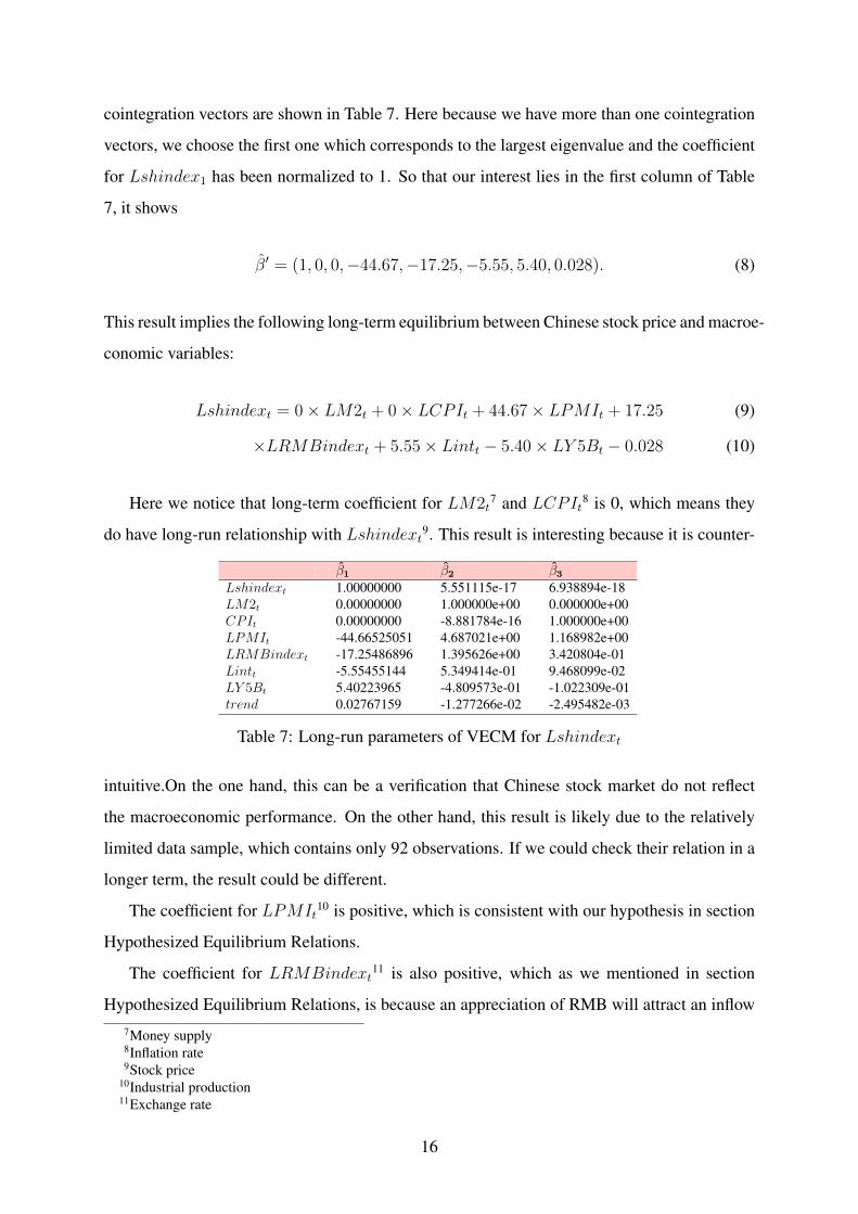
cointegration vectors are shown in Table 7. Here because we have more than one cointegration

vectors, we choose the first one which corresponds to the largest eigenvalue and the coefficient

for Lshindex1 has been normalized to 1. So that our interest lies in the first column of Table

7, it shows

β′ = (1, 0, 0,−44.67,−17.25,−5.55, 5.40, 0.028). (8)

This result implies the following long-term equilibrium between Chinese stock price and macroe-

conomic variables:

Lshindext = 0× LM2t + 0× LCPIt + 44.67× LPMIt + 17.25 (9)

×LRMBindext + 5.55× Lintt − 5.40× LY 5Bt − 0.028 (10)

Here we notice that long-term coefficient for LM2t7 and LCPIt8 is 0, which means they

do have long-run relationship with Lshindext9. This result is interesting because it is counter-

β1 β2 β3Lshindext 1.00000000 5.551115e-17 6.938894e-18LM2t 0.00000000 1.000000e+00 0.000000e+00CPIt 0.00000000 -8.881784e-16 1.000000e+00LPMIt -44.66525051 4.687021e+00 1.168982e+00LRMBindext -17.25486896 1.395626e+00 3.420804e-01Lintt -5.55455144 5.349414e-01 9.468099e-02LY 5Bt 5.40223965 -4.809573e-01 -1.022309e-01trend 0.02767159 -1.277266e-02 -2.495482e-03

Table 7: Long-run parameters of VECM for Lshindext

intuitive.On the one hand, this can be a verification that Chinese stock market do not reflect

the macroeconomic performance. On the other hand, this result is likely due to the relatively

limited data sample, which contains only 92 observations. If we could check their relation in a

longer term, the result could be different.

The coefficient for LPMIt10 is positive, which is consistent with our hypothesis in section

Hypothesized Equilibrium Relations.

The coefficient for LRMBindext11 is also positive, which as we mentioned in section

Hypothesized Equilibrium Relations, is because an appreciation of RMB will attract an inflow7Money supply8Inflation rate9Stock price

10Industrial production11Exchange rate

16

of foreign currency, which stimulate the whole economy, and drive the stock price high.

For interest rate, the result is interesting. We assume there is a negative relationship between

stock price and interest rate in previous section. Here we notice that this assumption is verified

by long-term interest rate LY 5Bt. However, for short-term interest rate Lintt, this is not the

case. Actually, this finding is consistent with Mukherjee and Naka’s (1995) and Maysami

and Koh’s (2000) findings in Japanese stock market and Singapore stock market respectively.

Mukherjee and Naka (1995) think this is because long-run interest rate LY 5Bt is likely to serve

as a better proxy variable for the risk-free component in the asset pricing model.

Then we need to test if the the long-run parameters β′ are significant, in order to do this,

we conduct a likelihood ratio test that has been introduced in section Methodology, the result

is shown in Table 8. The result indicates that long-run parameters β′ are significant for all

Null hypothesis: β1 = 0 β2 = 0 β3 = 0 β4 = 0 β5 = 0 β6 = 0 β7 = 0Test statistics 29.81 36.45 15.23 25.43 25.43 18.71 9.43p value 0 0 0 0 0 0 0.02

Table 8: Likelihood ratio test for restrictions on β

the variables at 5% significance level. This result is a violation of the result we got in Table,

since we found earlier that the long-term coefficients for LM2t and LCPIt are actually 0. This

could be a sign of misspecification of the basic VAR model and the long-term coefficients for

Lshindext, LM2t and LCPIt is likely to be insignificant. We’ll check this later in section

with VAR(2).

5.4 VECM Based On VAR(2)

As mentioned in last section, the contradiction of the point estimates of long-term coeffi-

cients β and their likelihood ratio test implies a misspecification of the model. Now we use the

VAR(2) to construct VECM. Maximum eigenvalue test λmax and the trace test λtrace in Table

9 shows there are only 1 cointegration vector.

Now we get the long-term β and corresponding p-value of likelihood ratio test. The result

is shown in Table 10. We have the following long-term relationship between stock price and

macroeconomic variables:

Lshindext = 10.1× LM2t − 108.9× LCPIt + 34.9× LPMIt + 9.9 (11)

×LRMBindext + 8.9× Lintt − 4.9× LY 5Bt + 0.09 (12)

17

h0 λ CV10% CV5% CV1%Trace Test

r <= 6 4.57 10.49 12.25 16.26r <= 5 12.20 22.76 25.32 30.45r <= 4 21.62 39.06 42.44 48.45r <= 3 36.07 59.14 62.99 70.05r <= 2 61.90 83.20 87.31 96.58r <= 1 106.80 110.42 114.90 124.75r = 0 180.66∗∗∗ 141.01 146.76 158.49

Maximum Eigenvalue Testr <= 6 4.57 10.49 12.25 16.26r <= 5 7.63 16.85 18.96 23.65r <= 4 9.42 23.11 25.54 30.34r <= 3 14.46 29.12 31.46 36.65r <= 2 25.82 34.75 37.52 42.36r <= 1 44.90∗∗ 40.91 43.97 49.51r = 0 73.86∗∗∗ 46.32 49.42 54.71

Table 9: Results and critical values for the λtrace and λmax test

We notice that although the signs of long-term relationship are consistent with our hy-

pothesis in section Hypothesized Equilibrium Relations, the coefficient for Lshindext is not

significant, this implies there is no significant long-term relationship between stock price and

macroeconomic variables although there may exist long-term equilibrium among economic

variables themselves.

Lshindext LM2t LCPIt LPMIt LRMBindext Lintt LY 5Bt

β 1 -10.1 108.9 -34.9 -9.9 -8.9 4.9p value 0.48 0.49 0 0 0.11 0 0

Table 10: β and corresponding p-value

5.5 Impulse Responses and Variance Decomposition

After getting the long-term relationship, our interest lies in the impulse responses and vari-

ance decomposition, which help explain how shocks transmit in the system and how much of

the variance of the forecast error of Lshindext is due to an exogenous shock to macroeconomic

variables. Here we use the VECM model based on VAR(5) to conduct impulse responses and

variance decomposition.

Figure 5 shows the responses of Lshindext to 6 macroeconomic variables together with

95% bootstrap confidence intervals base on 100 bootstrap replications. We notice that the point

estimate of long-term coefficients for LM2t and LCPIt in Table 7 are 0. But here we see in

Figure 5, a money supply shock εLM2t and a CPI shock εLCPIt lead to a negative and a positive

shock for stock price Lshindext respectively. This could be a proof of model no long-term

18

Figure 5: Responses of Lshindext to economic shocks with 95% confidence interval

equilibrium between stock price and 6 macroeconomic variables.

An industrial production shock εLPMIt has a positive shock for stock price Lshindext

reaching the maximum effect after about 10 months. A RMB currency exchange rate shock

εLRMBindext and a short-term interest rate shock εLinttalso have a positive shock for stock price

Lshindext reaching the maximum effect after about 7 months and 6 months respectively. A

long-term interest rate shock εLY 5Bt leads to a significant drop in Lshindext reaching the max-

imum effect after about 10 months. The sign of these four effect are consistent with the sign of

the estimate for long-term coefficients in Table 7 and Table 10.

Period Lshindext LM2t LCPIt LPMIt LRMBindext Lintt LY 5Bt

1 1.0000000 0.00000000 0.00000000 0.00000000 0.00000000 0.00000000 0.00000000

4 0.8813252 0.06103997 0.017813679 0.002314556 0.010792909 0.018064060 0.0086496683

8 0.7616360 0.11475628 0.018043496 0.012295687 0.023007225 0.028166457 0.0420948397

12 0.7424293 0.11405763 0.011792498 0.014530338 0.023738074 0.023351159 0.0701009829

24 0.7388168 0.11537311 0.007205497 0.012477996 0.026352095 0.019379647 0.0803948369

48 0.7354606 0.11674182 0.004503672 0.011612312 0.027329837 0.017517538 0.0868341996

Table 11: Forecast error variance decomposition of Lshindext

19

To assess the relative importance of the stock market shocks, we list forecast error variance

decomposition of stock price Lshindext for different horizons in Table 11. We notice that at

long-horizon, money supply LM2t and long-term interest rate LY 5Bt are vey important in

explaining the variance in stock price Lshindext. After s = 48, money supply shocks explain

about a fraction of 11.7% of the variance in stock price and long-term interest rate shocks

explain about a fraction of 8.7% of the variance in stock price.

6 Conclusion

This paper use Johansen’s VECM method to investigate the long-term equilibrium between

stock price and 6 macroeconomic variables in China. Using VAR(5) and VAR(2) to con-

struct VECM models respectively, we found there is no long-term equilibrium between stock

price and 6 macroeconomic variables, although there may exist long-term equilibrium among

macroeconomic variables themselves. However, this doesn’t mean that stock price cannot re-

flect the real economy. Impulse responses plots indicate although the effect of money supply

and inflation rate CPI on stock price are contradictory with hypothesis. Industrial production,

exchange rate and interest rate do have effect on stock price that are consistent with economic

hypothesis. In conclusion, we cannot say Chinese stock market isn’t the barometer of the real

economy.

References

[1] Johansen, S., & Juselius, K. (1990). Maximum likelihood estimation and inference on

cointegration with application to the demand for money. Oxford Bulletin of Economics

and Statistics 52, 169-210.

[2] Mukherjee, T. K., & Naka, A. (1995). Dynamic relations between macroeconomic vari-

ables and the Japanese stock market: an application of a vector error correction model.

Journal of Financial Research, 18(2), 223-237.

[3] Chen, N., Roll, R., & Ross, S. (1986). Economic Forces and the Stock Market. The Jour-

nal of Business, 59(3), 383-403.

20

[4] Engle, R. E., & Granger, C. (1987). Cointegration and error-correction: representation,

estimation and testing. Econometrica 55, 251-276.

[5] Johansen, S. (1988). Statistical analysis of cointegration vectors. Journal of economic

dynamics and control, 12(2-3), 231-254.

[6] Lütkepohl, H. K. M. P. P. (2004). Applied Time Series Econometrics. Cambridge: Cam-

bridge University Press.

[7] Fama, E. F., & Schwert, W. G. (1977). Asset returns and inflation. Journal of Financial

Economics 5, 115-146.

[8] Geske, R., & Roll, R. (1983). The fiscal and monetary linkage between stock returns and

inflation. Journal of Finance 38, 7-33.

[9] Fisher, I. (1930). Theory of interest. Augustus M Kelley publishers.

[10] Johansen, S. (1991). Estimation and hypothesis testing of cointegration vectors in Gaus-

sian vector autoregressive models. Econometrica: Journal of the Econometric Society,

1551-1580.

[11] Liu, M. H., & Shrestha, K. M. (2008). Analysis of the long-term relationship between

macro-economic variables and the Chinese stock market using heteroscedastic cointegra-

tion. Managerial Finance, 34(11), 744-755.

[12] Fama, E. F. (1981). Stock returns, real activity, inflation and money. The American Eco-

nomic Review 71, 545-565.

[13] Ross, S.A. (1976). The arbitrage theory of capital asset pricing. Journal of Economic

Theory 13, 341-360.

[14] Pfaff, B. (2008). Analysis of integrated and cointegrated time series with R. Springer

Science & Business Media.

[15] Pfaff, B. (2008). VAR, SVAR and SVEC models: Implementation within R package vars.

Journal of Statistical Software, 27(4), 1-32.

[16] Maysami, R. C., & Koh, T. S. (2000). A vector error correction model of the Singapore

stock market. International Review of Economics & Finance, 9(1), 79-96.

21

[17] Hamilton, J. D. (1994). Time series analysis (Vol. 2). Princeton: Princeton university

press.

22