Embed Size (px)
DESCRIPTION
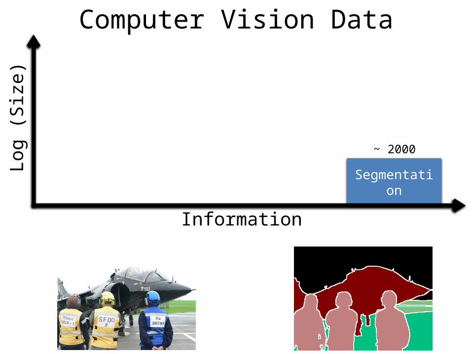
Loss-based Learning with Weak Supervision. M. Pawan Kumar. Computer Vision Data. Log (Size). ~ 2000. Segmentation. Information. Computer Vision Data. ~ 1 M. Log (Size). Bounding Box. ~ 2000. Segmentation. Information. Computer Vision Data. > 14 M. ~ 1 M. Log (Size). Image-Level. - PowerPoint PPT Presentation
Citation preview
Loss-based Learning with Weak Supervision
M. Pawan Kumar
Segmentation
Information
Log (
Siz
e)
~ 2000
Computer Vision Data
Segmentation
Log (
Siz
e)
~ 2000
Information
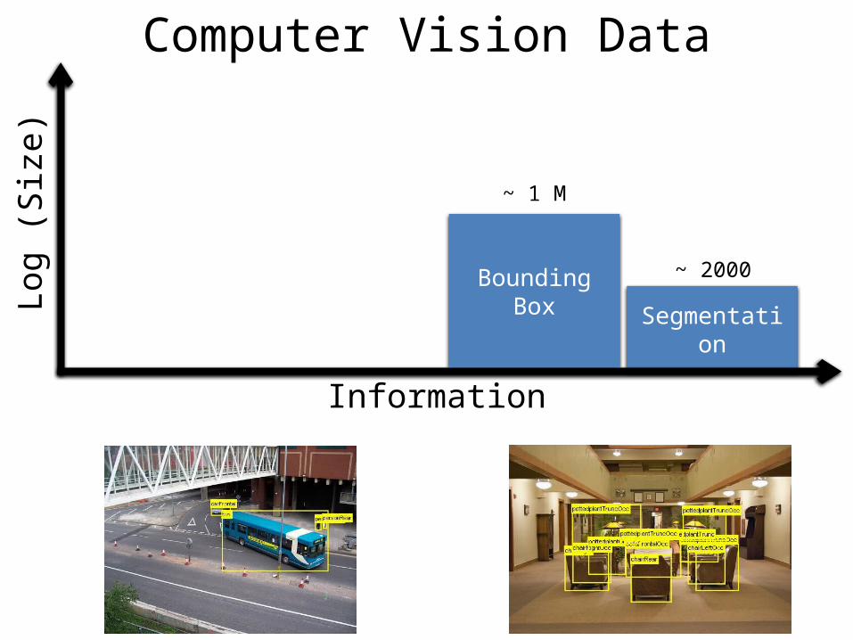
Bounding Box
~ 1 M
Computer Vision Data
Segmentation
Log (
Siz
e)
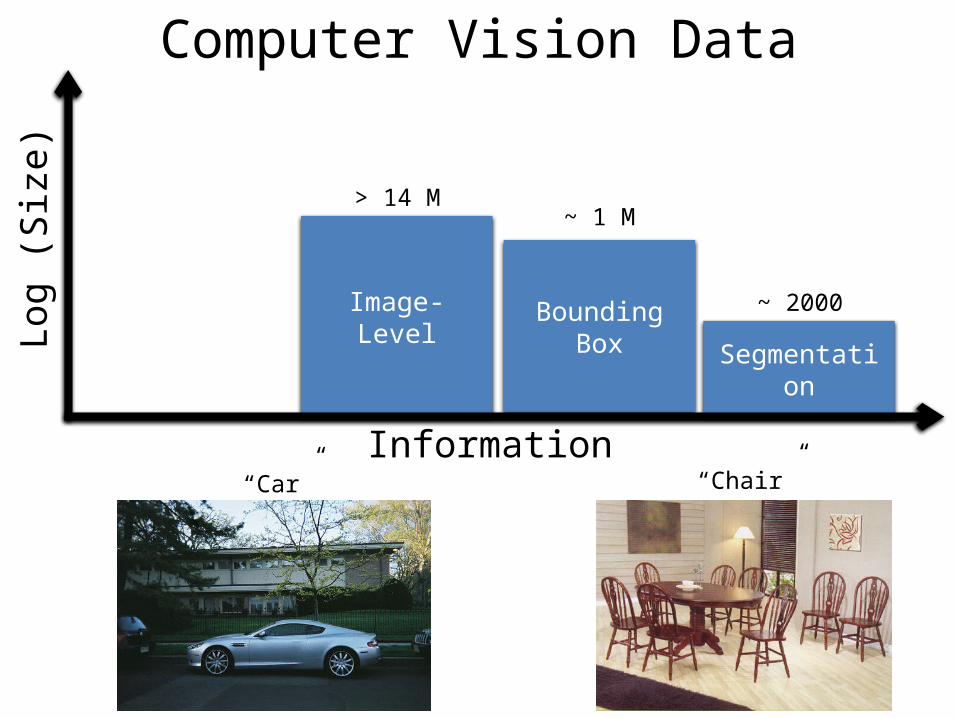
Bounding BoxImage-Level~ 2000
~ 1 M> 14 M
“Car” “Chair”Information
Computer Vision Data
Segmentation
Log (
Siz
e)
Image-Level
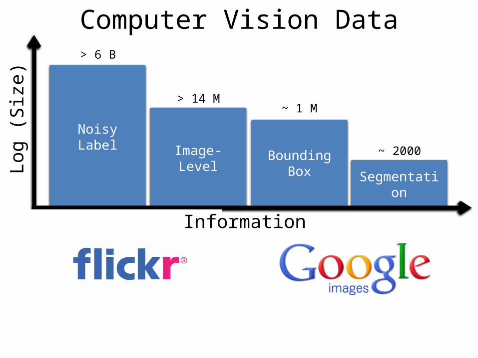
Noisy Label~ 2000
> 14 M
> 6 B
Information
Bounding Box
~ 1 M
Computer Vision Data
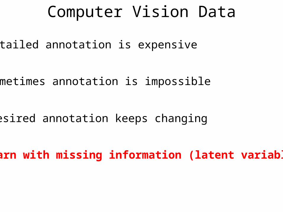
Learn with missing information (latent variables)
Detailed annotation is expensive
Sometimes annotation is impossible
Desired annotation keeps changing
Computer Vision Data
• Two Types of Problems
• Part I – Annotation Mismatch
• Part II – Output Mismatch
Outline
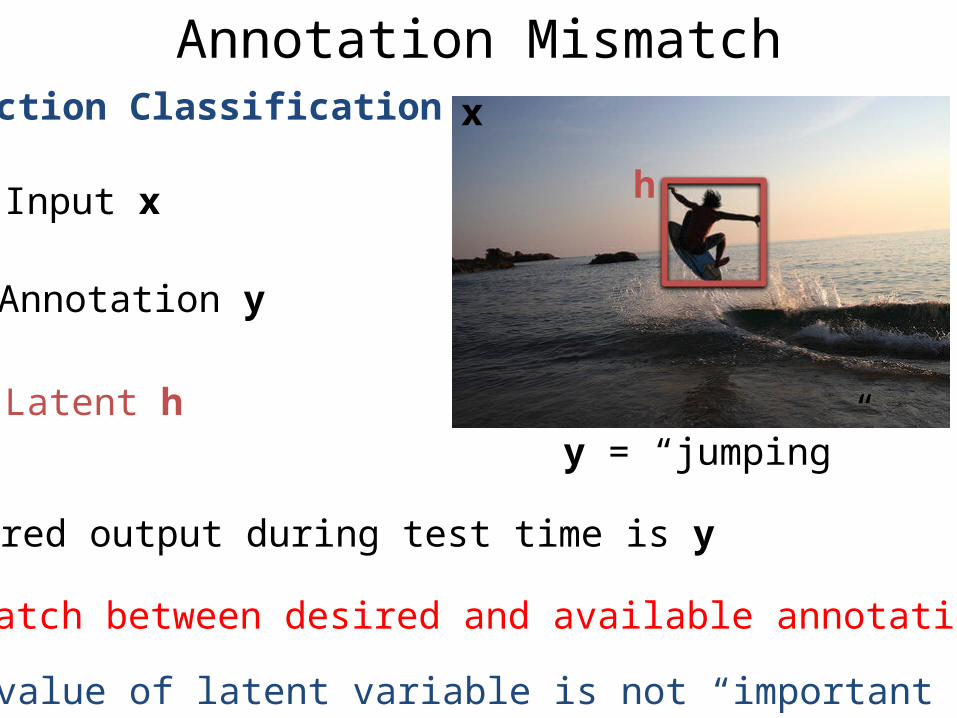
Annotation Mismatch
Input x
Annotation y
Latent h
x
y = “jumping”
h
Action Classification
Mismatch between desired and available annotations
Exact value of latent variable is not “important”
Desired output during test time is y
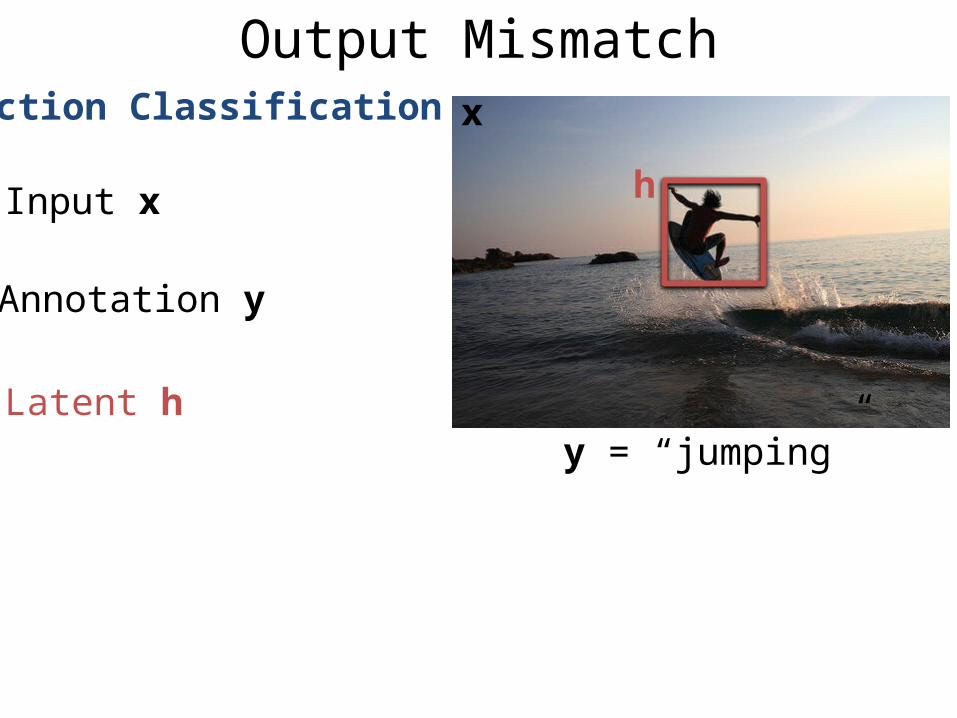
Output Mismatch
Input x
Annotation y
Latent h
x
y = “jumping”
h
Action Classification

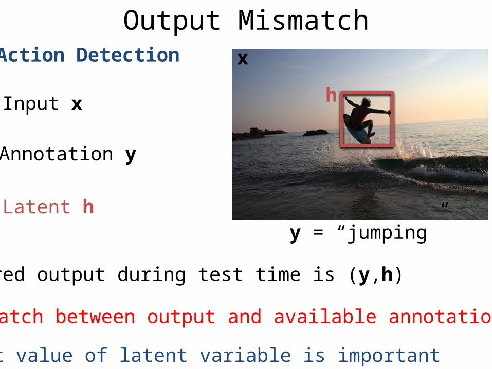
Output Mismatch
Input x
Annotation y
Latent h
x
y = “jumping”
h
Action Detection
Mismatch between output and available annotations
Exact value of latent variable is important
Desired output during test time is (y,h)

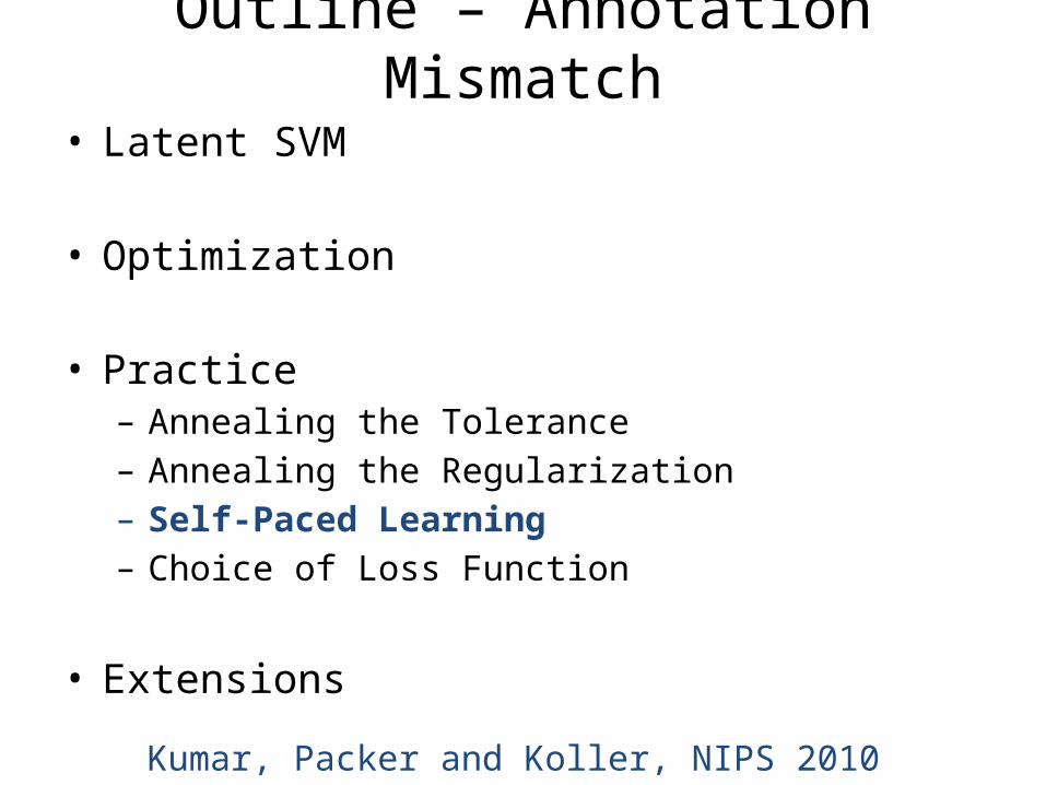
Part I
• Latent SVM
• Optimization
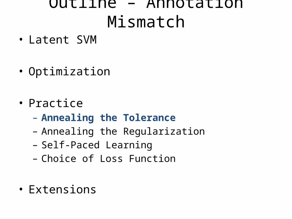
• Practice
• Extensions
Outline – Annotation Mismatch
Andrews et al., NIPS 2001; Smola et al., AISTATS 2005;Felzenszwalb et al., CVPR 2008; Yu and Joachims, ICML 2009

Weakly Supervised Data
Input x
Output y {-1,+1}
Hidden h
x
y = +1
h

Weakly Supervised Classification
Feature Φ(x,h)
Joint Feature Vector
Ψ(x,y,h)
x
y = +1
h
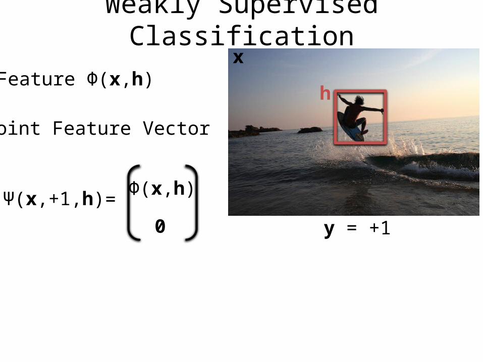
Weakly Supervised Classification
Feature Φ(x,h)
Joint Feature Vector
Ψ(x,+1,h) Φ(x,h)
0
=
x
y = +1
h
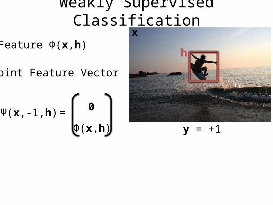
Weakly Supervised Classification
Feature Φ(x,h)
Joint Feature Vector
Ψ(x,-1,h) 0
Φ(x,h)
=
x
y = +1
h
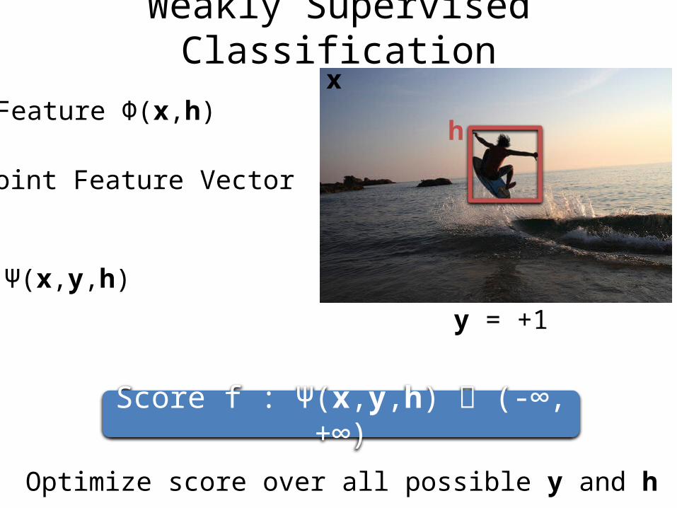
Weakly Supervised Classification
Feature Φ(x,h)
Joint Feature Vector
Ψ(x,y,h)
Score f : Ψ(x,y,h) (-∞, +∞)
Optimize score over all possible y and h
x
y = +1
h
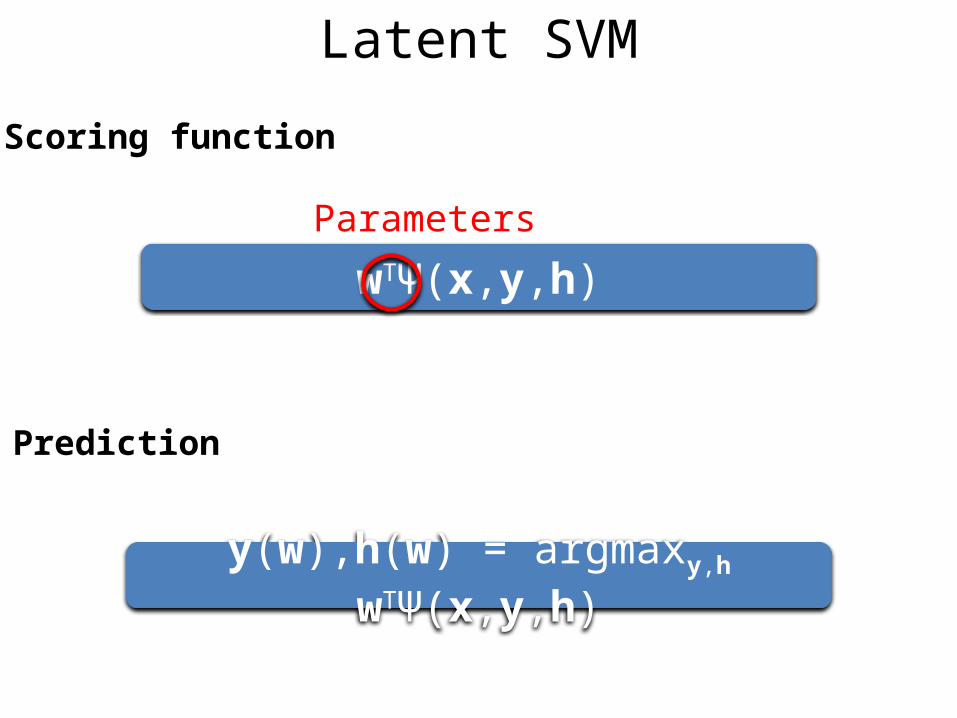
Scoring function
wTΨ(x,y,h)
Prediction
y(w),h(w) = argmaxy,h wTΨ(x,y,h)
Latent SVM
Parameters
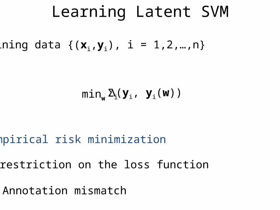
Learning Latent SVM
(yi, yi(w))Σi
Empirical risk minimization
minw
No restriction on the loss function
Annotation mismatch
Training data {(xi,yi), i = 1,2,…,n}
Learning Latent SVM
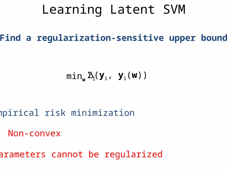
(yi, yi(w))Σi
Empirical risk minimization
minw
Non-convex
Parameters cannot be regularized
Find a regularization-sensitive upper bound
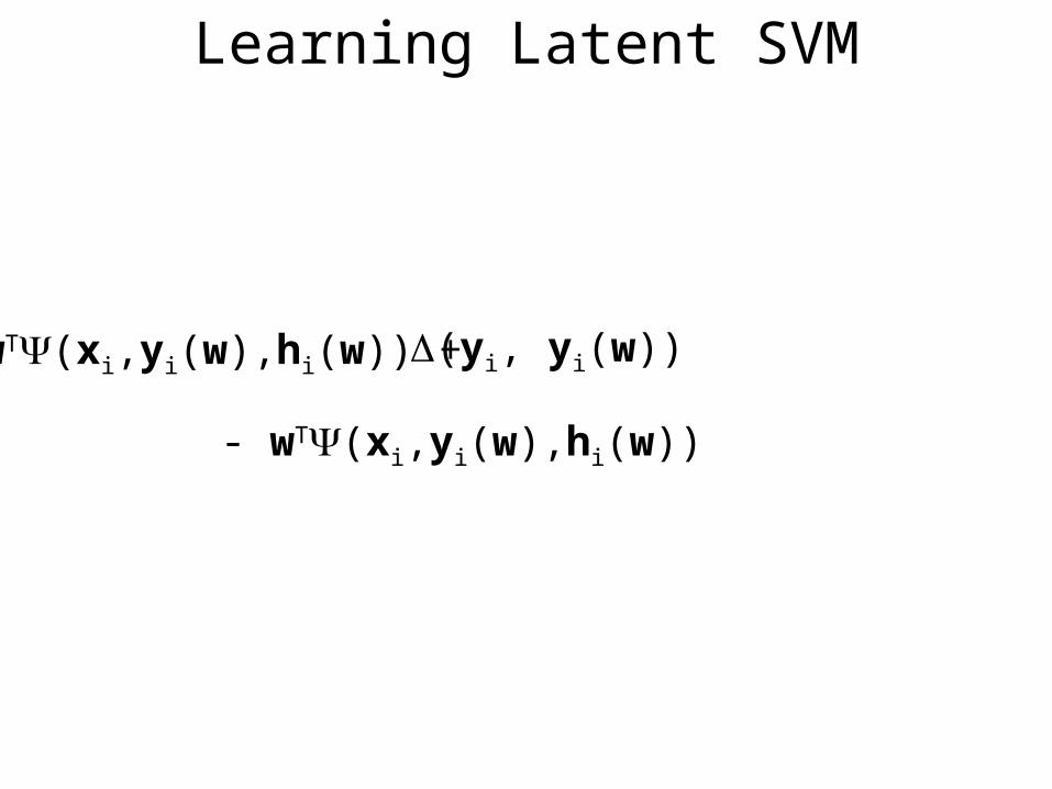
Learning Latent SVM
- wT(xi,yi(w),hi(w))
(yi, yi(w))wT(xi,yi(w),hi(w)) +
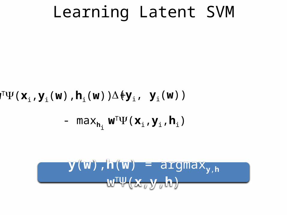
Learning Latent SVM
(yi, yi(w))wT(xi,yi(w),hi(w)) +
- maxhi wT(xi,yi,hi)
y(w),h(w) = argmaxy,h wTΨ(x,y,h)
Learning Latent SVM
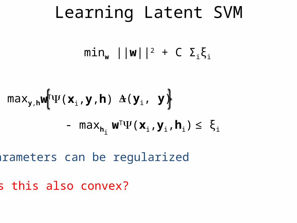
(yi, y)wT(xi,y,h) +maxy,h
- maxhi wT(xi,yi,hi) ≤ ξi
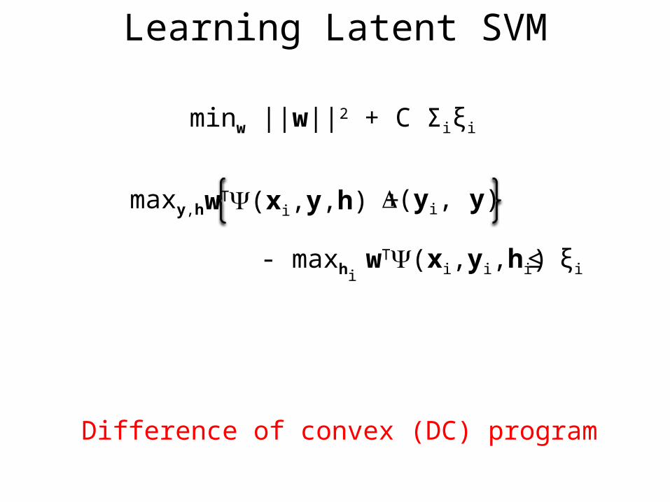
minw ||w||2 + C Σiξi
Parameters can be regularized
Is this also convex?
Learning Latent SVM
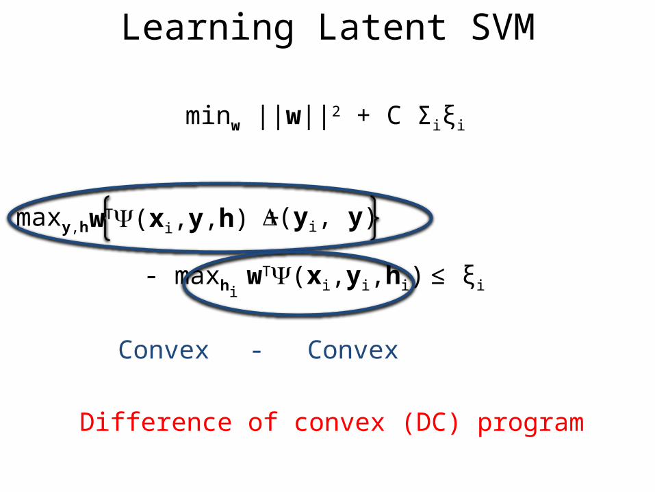
(yi, y)wT(xi,y,h) +maxy,h
- maxhi wT(xi,yi,hi) ≤ ξi
minw ||w||2 + C Σiξi
Convex Convex-
Difference of convex (DC) program
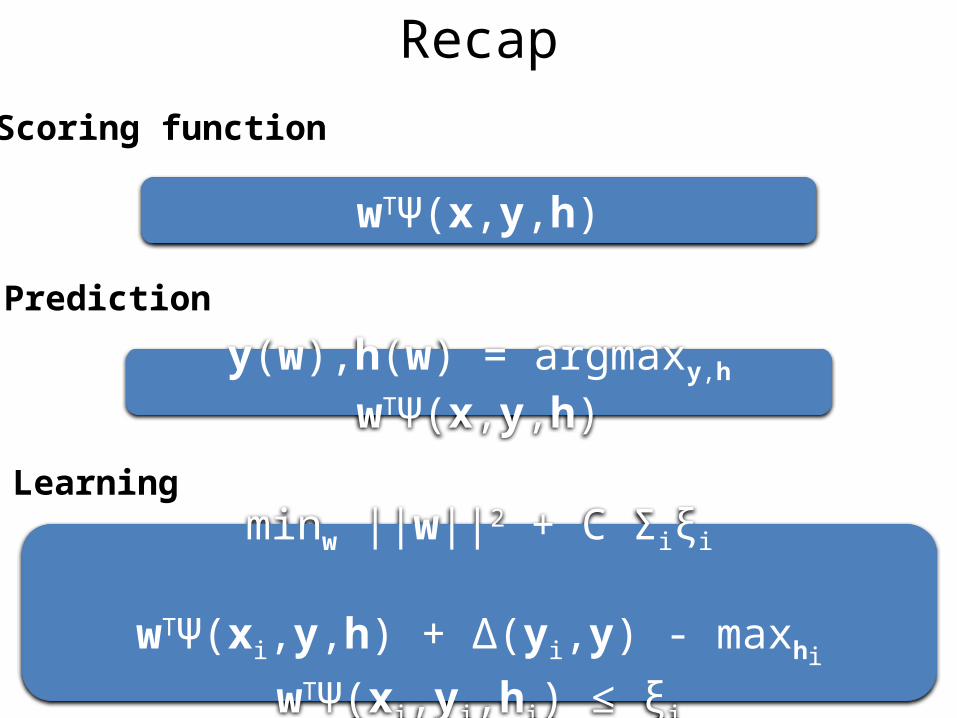
minw ||w||2 + C Σiξi
wTΨ(xi,y,h) + Δ(yi,y) - maxhi wTΨ(xi,yi,hi) ≤ ξi
Scoring function
wTΨ(x,y,h)
Prediction
y(w),h(w) = argmaxy,h wTΨ(x,y,h)
Learning
Recap
• Latent SVM
• Optimization
• Practice
• Extensions
Outline – Annotation Mismatch
Learning Latent SVM
(yi, y)wT(xi,y,h) +maxy,h
- maxhi wT(xi,yi,hi) ≤ ξi
minw ||w||2 + C Σiξi
Difference of convex (DC) program
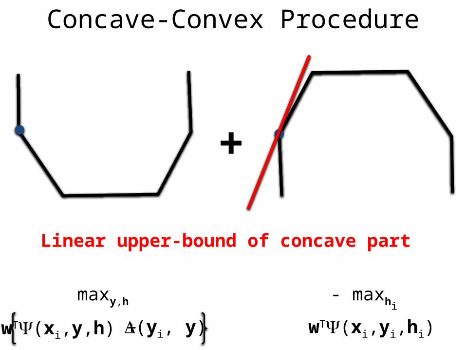
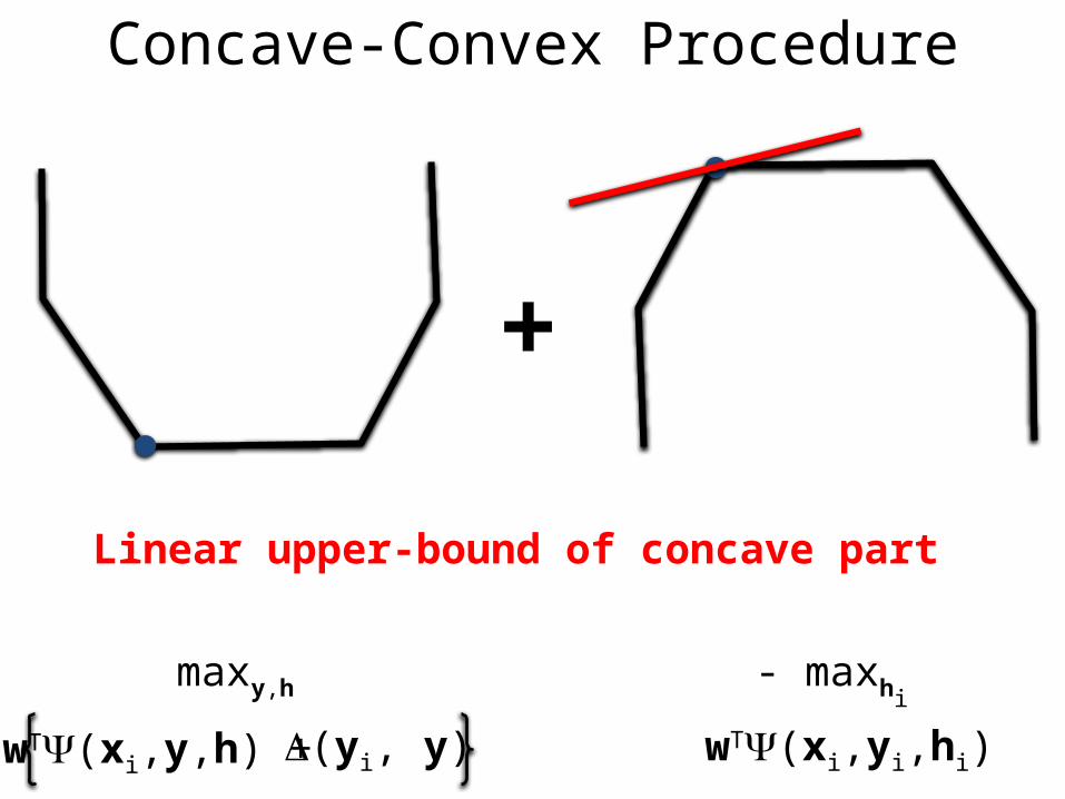
Concave-Convex Procedure
+
(yi, y)wT(xi,y,h) +
maxy,h
wT(xi,yi,hi)
- maxhi
Linear upper-bound of concave part
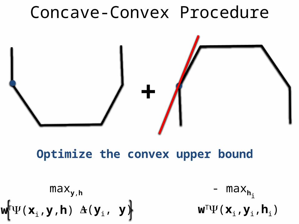
Concave-Convex Procedure
+
(yi, y)wT(xi,y,h) +
maxy,h
wT(xi,yi,hi)
- maxhi
Optimize the convex upper bound
Concave-Convex Procedure
+
(yi, y)wT(xi,y,h) +
maxy,h
wT(xi,yi,hi)
- maxhi
Linear upper-bound of concave part
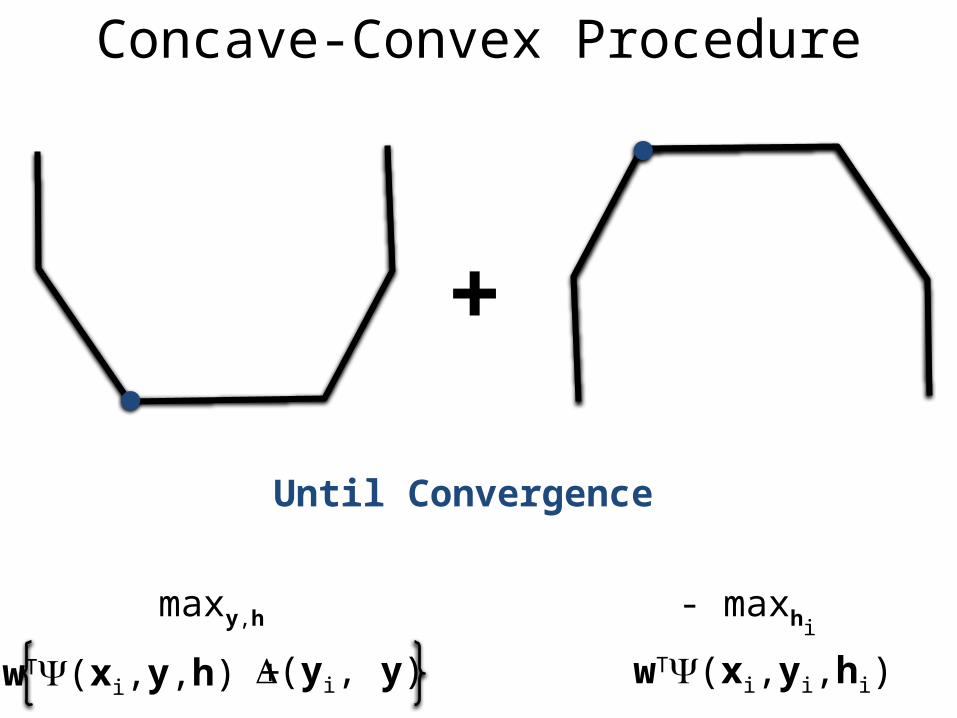
Concave-Convex Procedure
+
(yi, y)wT(xi,y,h) +
maxy,h
wT(xi,yi,hi)
- maxhi
Until Convergence
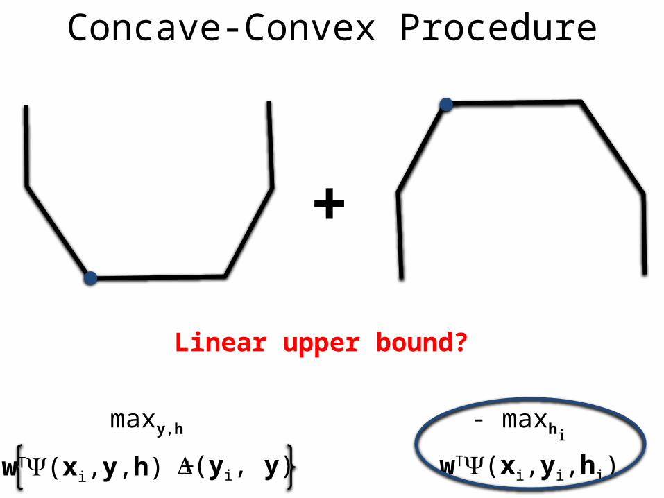
Concave-Convex Procedure
+
(yi, y)wT(xi,y,h) +
maxy,h
wT(xi,yi,hi)
- maxhi
Linear upper bound?
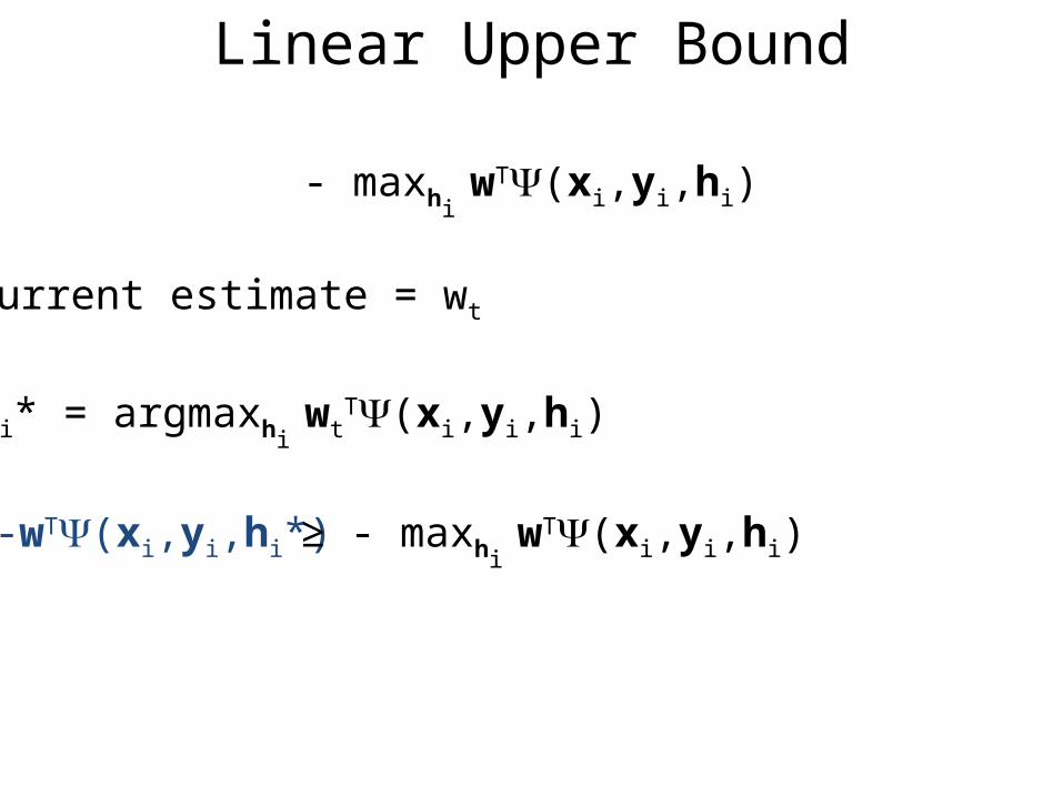
Linear Upper Bound
- maxhi wT(xi,yi,hi)
-wT(xi,yi,hi*)
hi* = argmaxhi wt
T(xi,yi,hi)
Current estimate = wt
≥ - maxhi wT(xi,yi,hi)
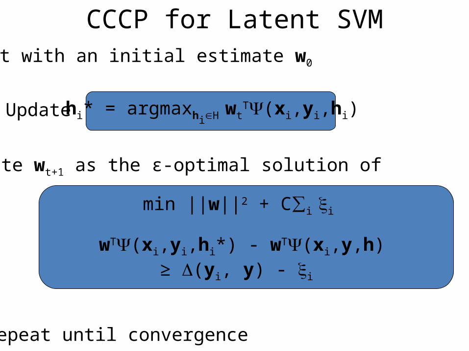
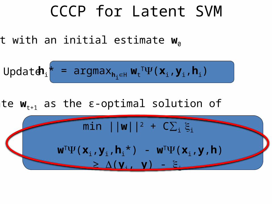
CCCP for Latent SVMStart with an initial estimate w0
Update
Update wt+1 as the ε-optimal solution of
min ||w||2 + C∑i i
wT(xi,yi,hi*) - wT(xi,y,h)≥ (yi, y) - i
hi* = argmaxhiH wtT(xi,yi,hi)
Repeat until convergence
• Latent SVM
• Optimization
• Practice
• Extensions
Outline – Annotation Mismatch
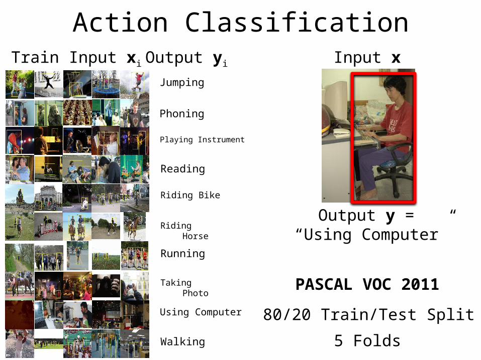
Action ClassificationInput x
Output y = “Using Computer”
PASCAL VOC 2011
80/20 Train/Test Split
5 Folds
Jumping
Phoning
Playing Instrument
Reading
Riding Bike
Riding Horse
Running
Taking Photo
Using Computer
Walking
Train Input xi Output yi
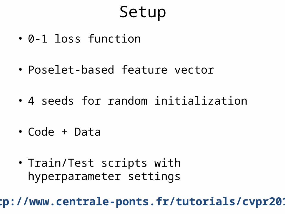
• 0-1 loss function
• Poselet-based feature vector
• 4 seeds for random initialization
• Code + Data
• Train/Test scripts with hyperparameter settings
Setup
http://www.centrale-ponts.fr/tutorials/cvpr2013/
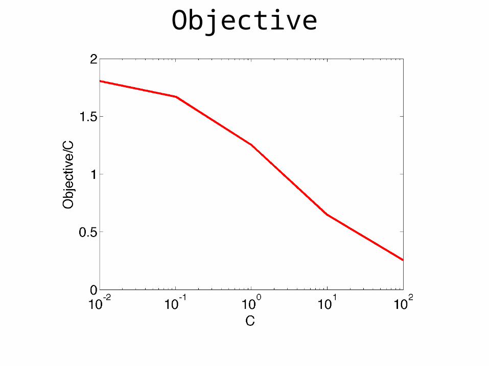
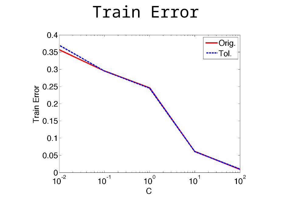
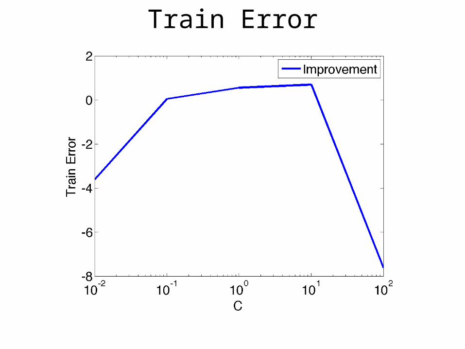
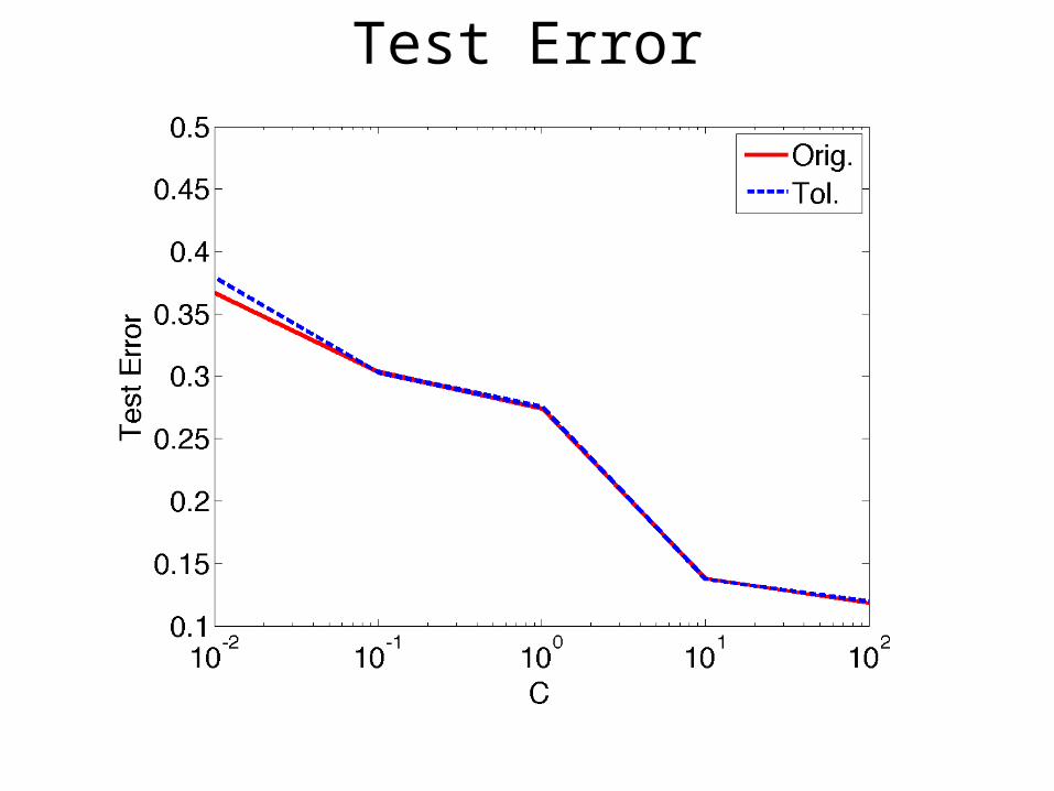
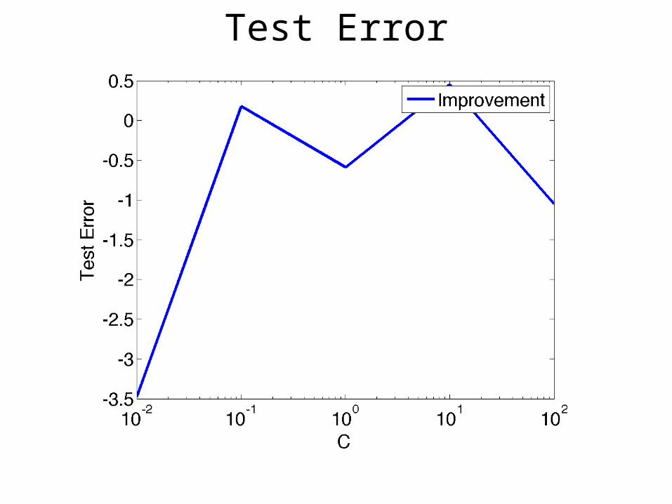
Objective
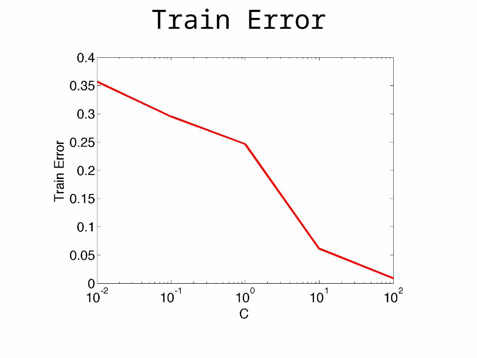
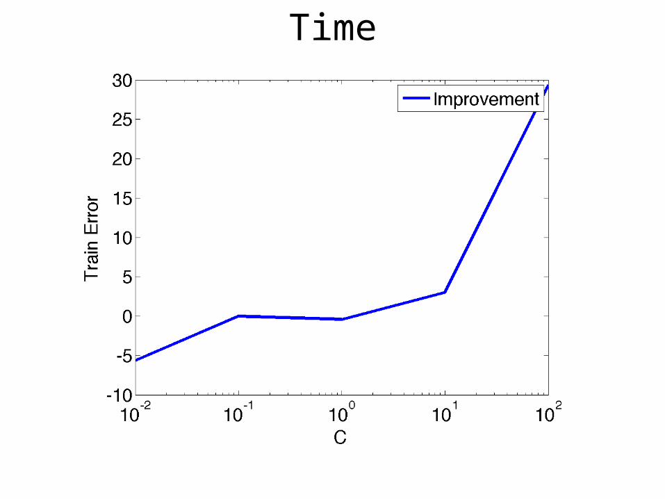
Train Error
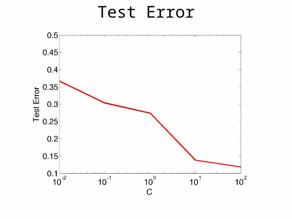
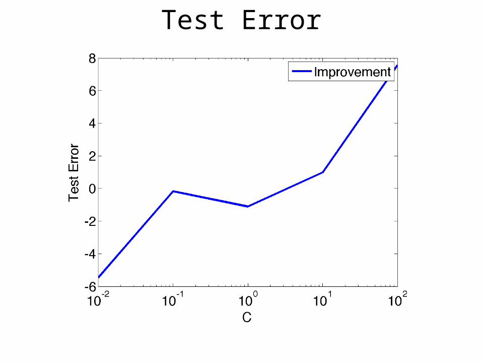
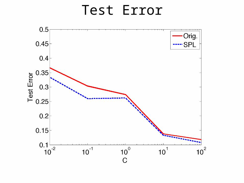
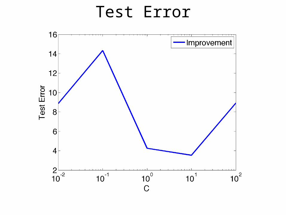
Test Error
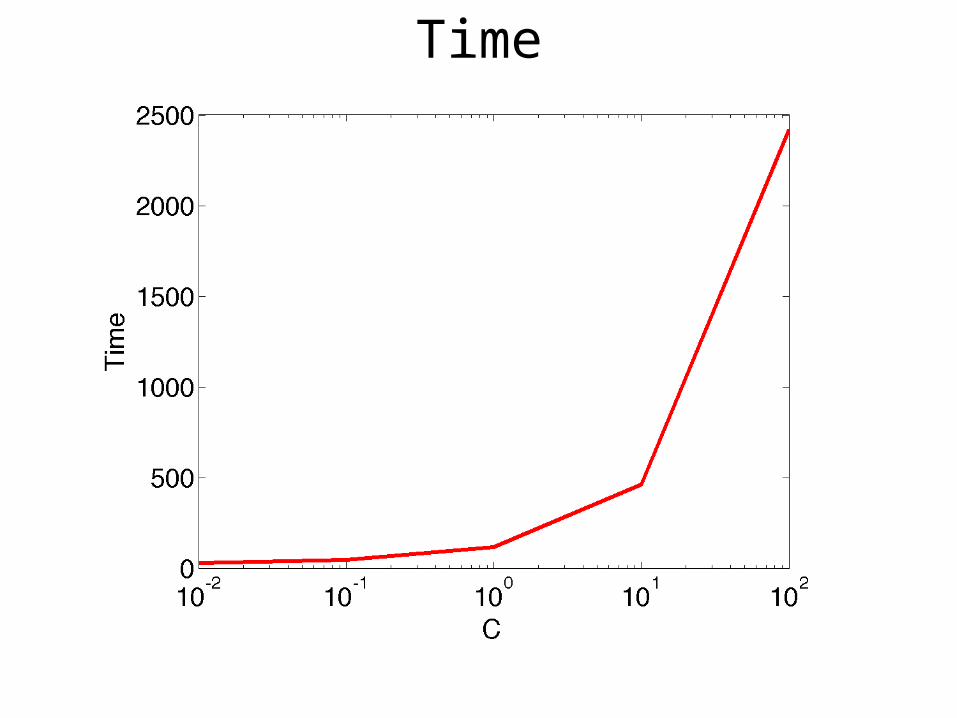
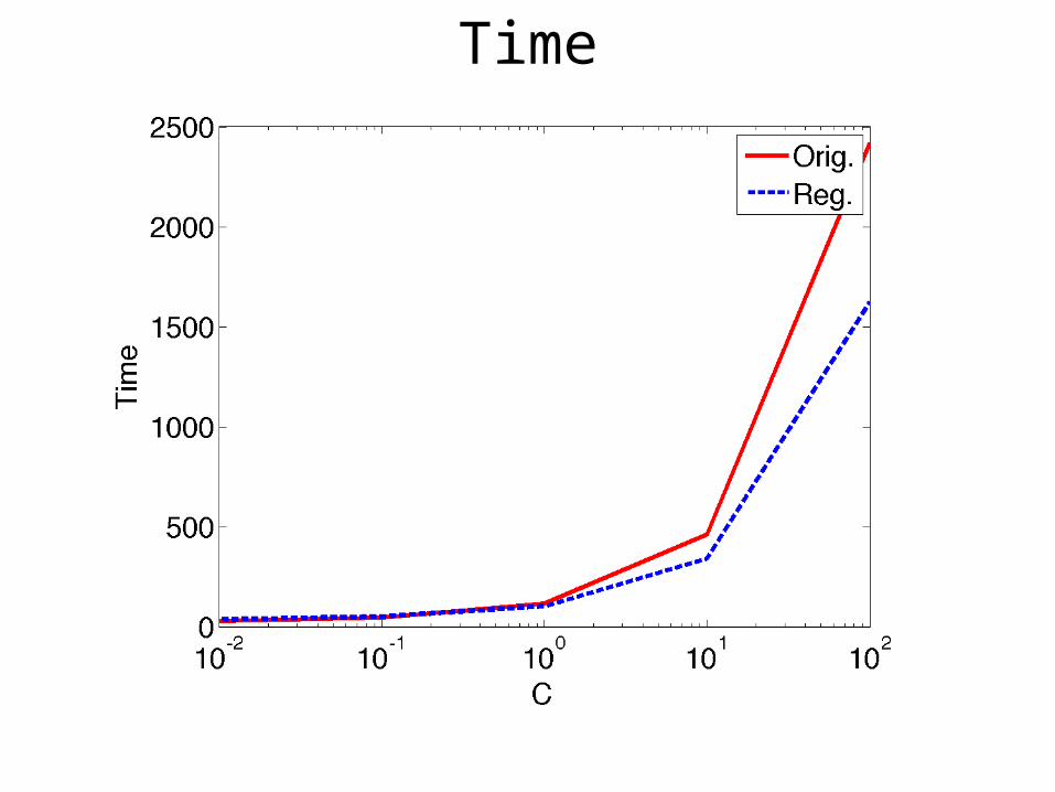
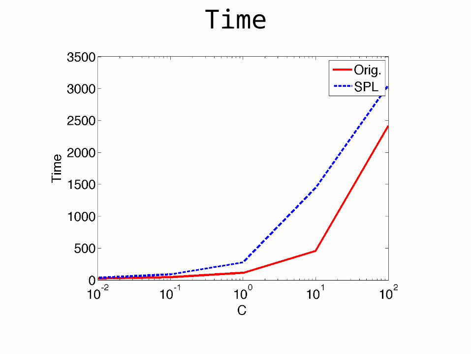
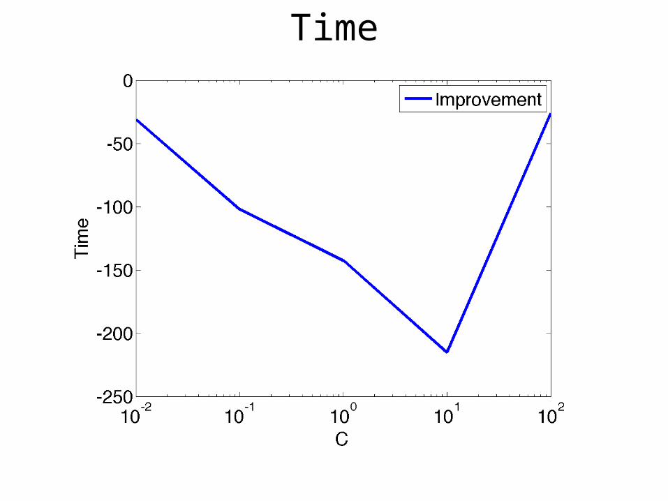
Time
• Latent SVM
• Optimization
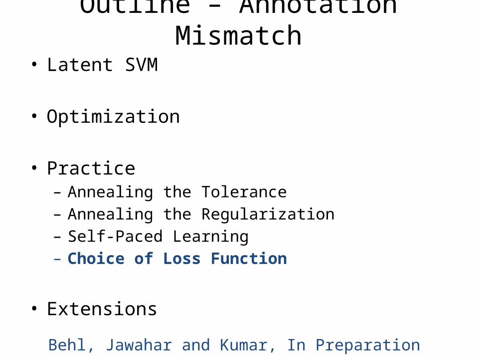
• Practice– Annealing the Tolerance– Annealing the Regularization– Self-Paced Learning– Choice of Loss Function
• Extensions
Outline – Annotation Mismatch

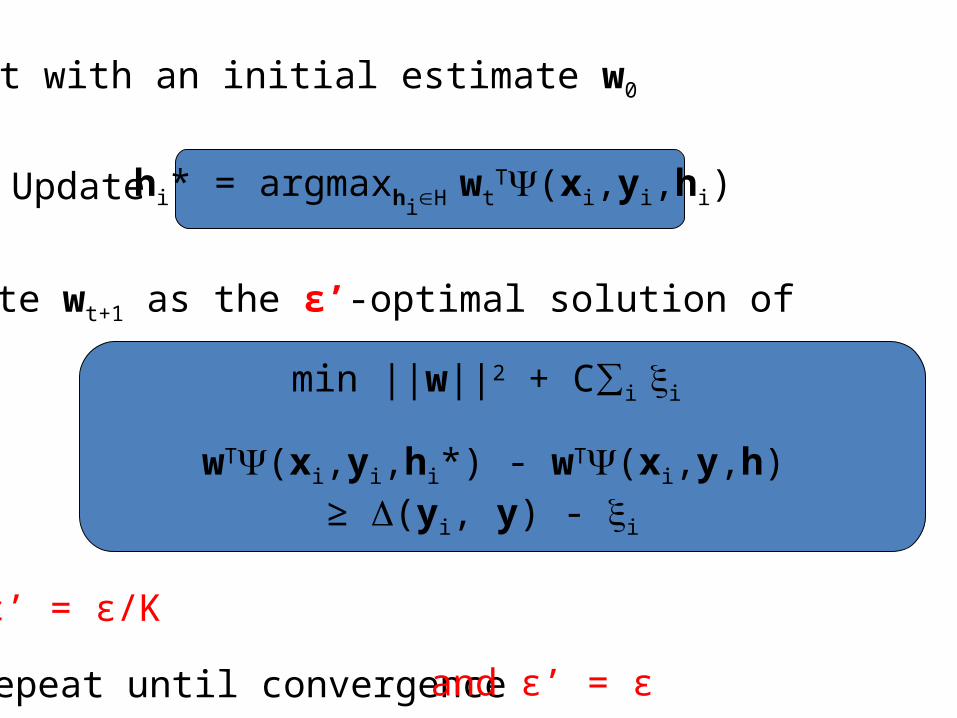
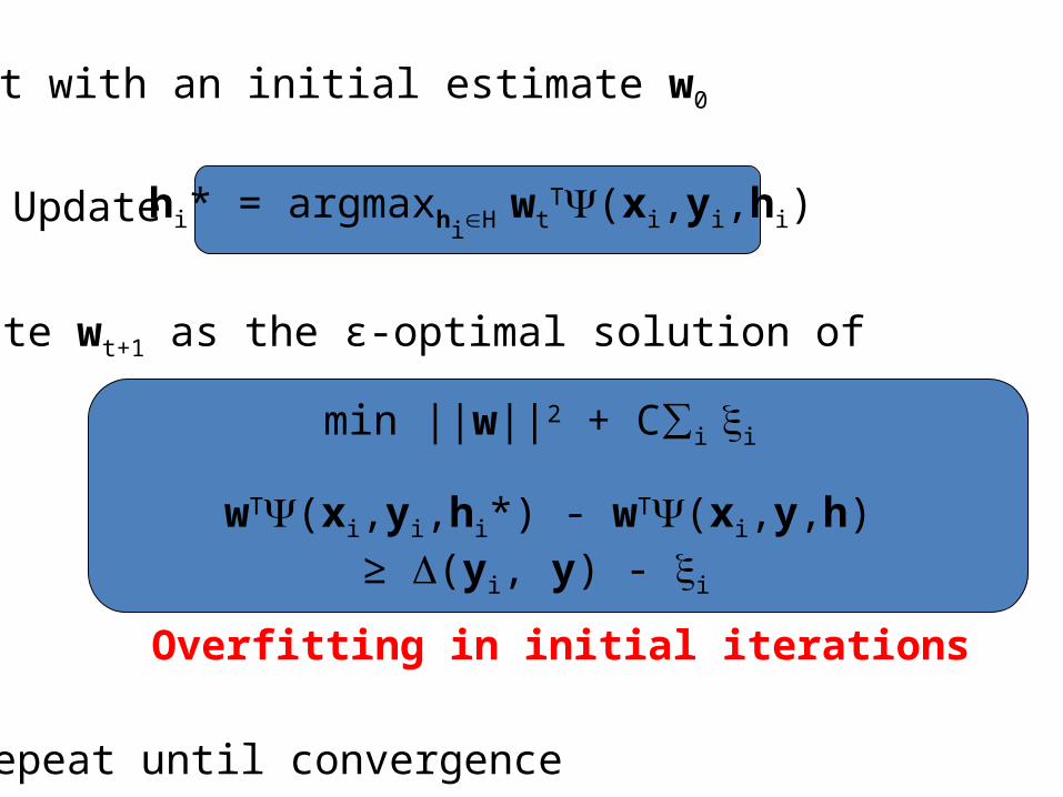
Start with an initial estimate w0
Update
Update wt+1 as the ε-optimal solution of
min ||w||2 + C∑i i
wT(xi,yi,hi*) - wT(xi,y,h)≥ (yi, y) - i
hi* = argmaxhiH wtT(xi,yi,hi)
Repeat until convergence
Overfitting in initial iterations
Repeat until convergence
ε’ = ε/K
and ε’ = ε
Start with an initial estimate w0
Update
Update wt+1 as the ε’-optimal solution of
min ||w||2 + C∑i i
wT(xi,yi,hi*) - wT(xi,y,h)≥ (yi, y) - i
hi* = argmaxhiH wtT(xi,yi,hi)
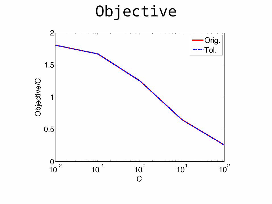
Objective
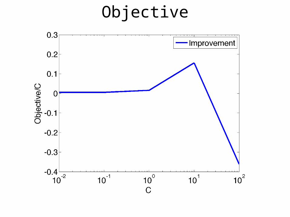
Objective
Train Error
Train Error
Test Error
Test Error
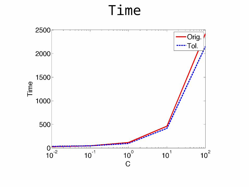
Time
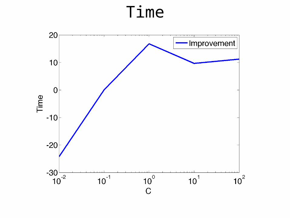
Time

• Latent SVM
• Optimization
• Practice– Annealing the Tolerance– Annealing the Regularization– Self-Paced Learning– Choice of Loss Function
• Extensions
Outline – Annotation Mismatch
Start with an initial estimate w0
Update
Update wt+1 as the ε-optimal solution of
min ||w||2 + C∑i i
wT(xi,yi,hi*) - wT(xi,y,h)≥ (yi, y) - i
hi* = argmaxhiH wtT(xi,yi,hi)
Repeat until convergence
Overfitting in initial iterations

Repeat until convergence
C’ = C x K
and C’ = C
Start with an initial estimate w0
Update
Update wt+1 as the ε-optimal solution of
min ||w||2 + C’∑i i
wT(xi,yi,hi*) - wT(xi,y,h)≥ (yi, y) - i
hi* = argmaxhiH wtT(xi,yi,hi)
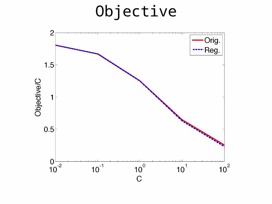
Objective
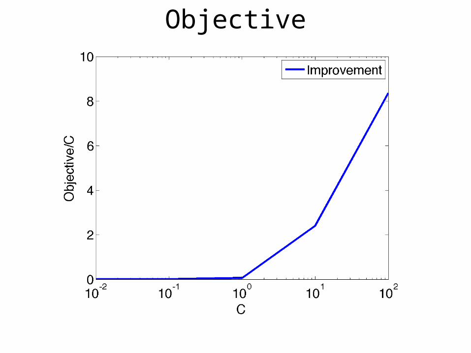
Objective
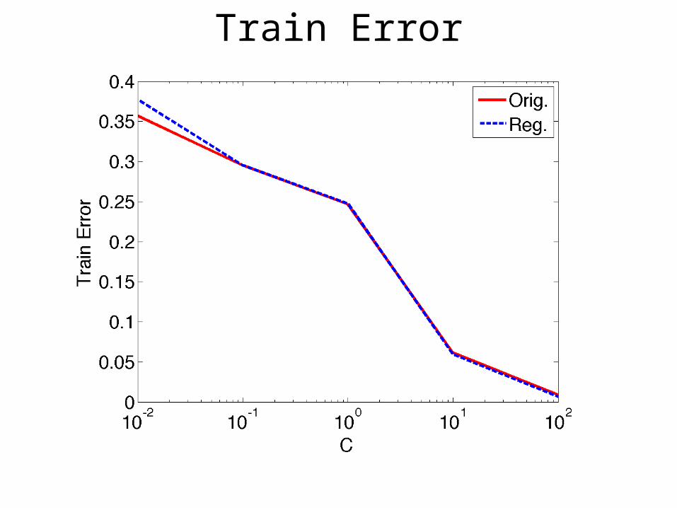
Train Error
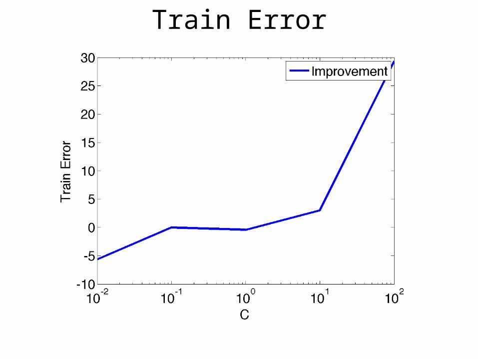
Train Error
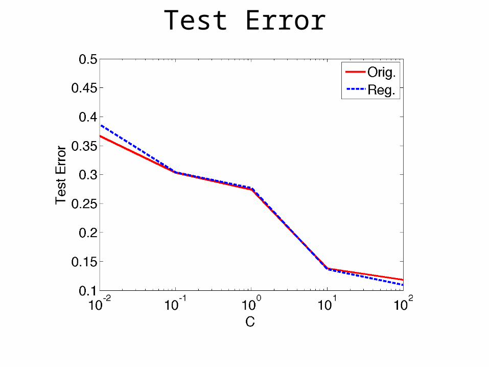
Test Error
Test Error
Time
Time
• Latent SVM
• Optimization
• Practice– Annealing the Tolerance– Annealing the Regularization– Self-Paced Learning– Choice of Loss Function
• Extensions
Outline – Annotation Mismatch
Kumar, Packer and Koller, NIPS 2010
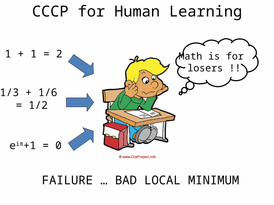
1 + 1 = 2
1/3 + 1/6 = 1/2
eiπ+1 = 0
Math is for losers !!
FAILURE … BAD LOCAL MINIMUM
CCCP for Human Learning
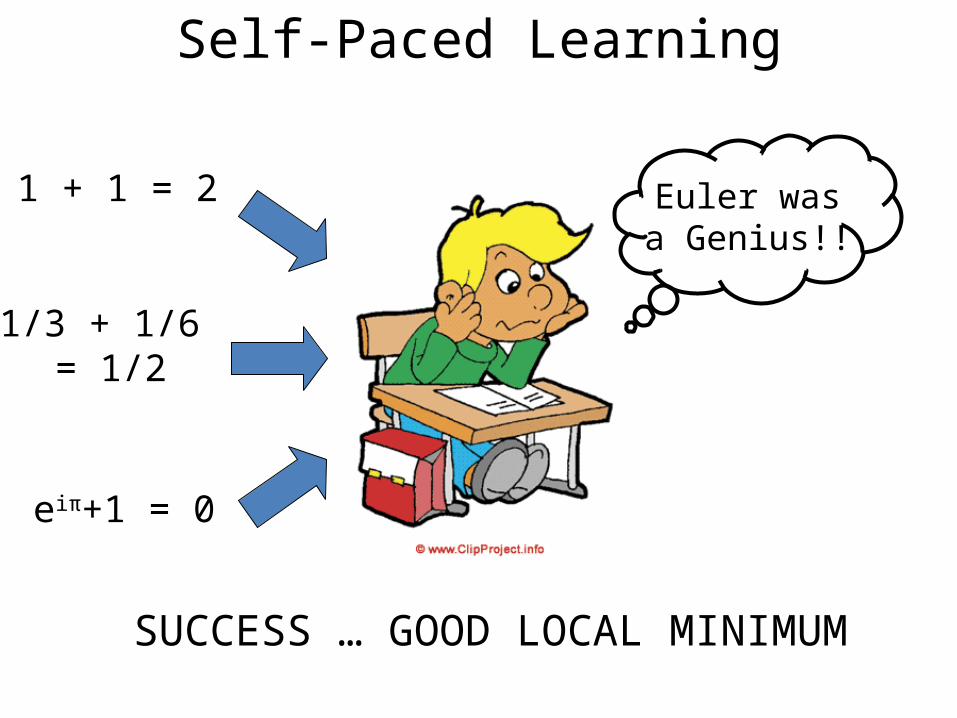
Euler wasa Genius!!
SUCCESS … GOOD LOCAL MINIMUM
1 + 1 = 2
1/3 + 1/6 = 1/2
eiπ+1 = 0
Self-Paced Learning
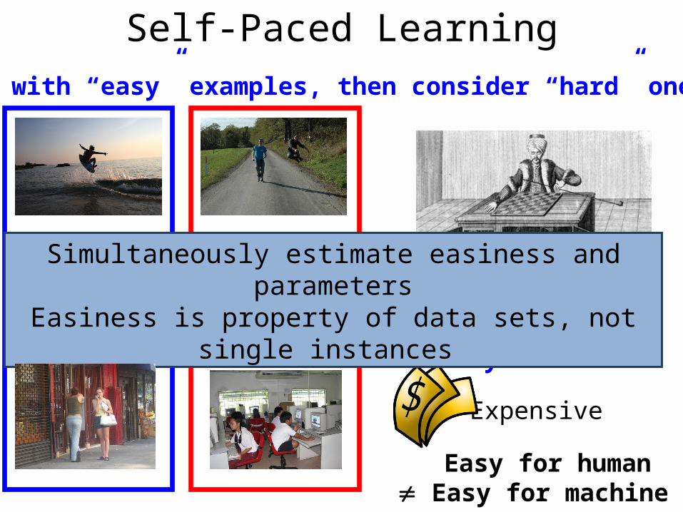
Start with “easy” examples, then consider “hard” ones
Easy vs. Hard
Expensive
Easy for human Easy for machine
Self-Paced Learning
Simultaneously estimate easiness and parametersEasiness is property of data sets, not single instances
Start with an initial estimate w0
Update
Update wt+1 as the ε-optimal solution of
min ||w||2 + C∑i i
wT(xi,yi,hi*) - wT(xi,y,h)≥ (yi, y) - i
hi* = argmaxhiH wtT(xi,yi,hi)
CCCP for Latent SVM
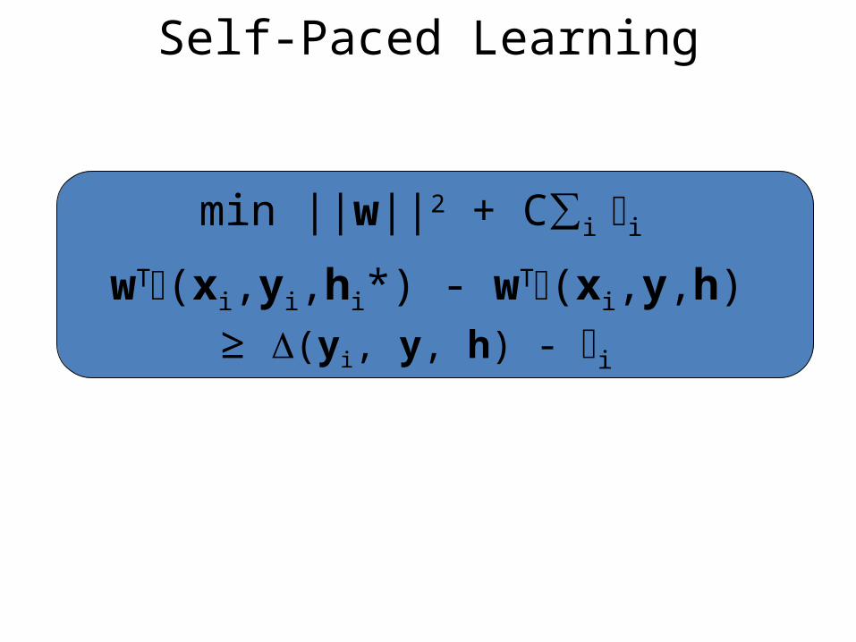
min ||w||2 + C∑i i
wT(xi,yi,hi*) - wT(xi,y,h)≥ (yi, y, h) - i
Self-Paced Learning

min ||w||2 + C∑i vii
wT(xi,yi,hi*) - wT(xi,y,h)≥ (yi, y, h) - i
vi {0,1}
Trivial Solution
Self-Paced Learning
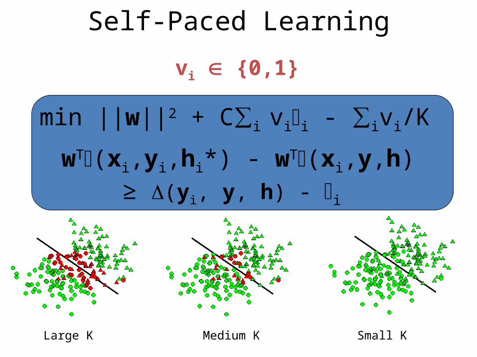
vi {0,1}
Large K Medium K Small K
min ||w||2 + C∑i vii - ∑ivi/K
wT(xi,yi,hi*) - wT(xi,y,h)≥ (yi, y, h) - i
Self-Paced Learning
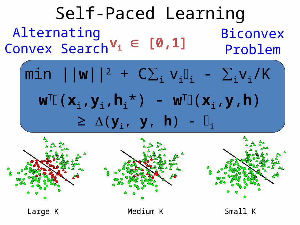
vi [0,1]
min ||w||2 + C∑i vii - ∑ivi/K
wT(xi,yi,hi*) - wT(xi,y,h)≥ (yi, y, h) - i
Large K Medium K Small K
BiconvexProblem
AlternatingConvex Search
Self-Paced Learning
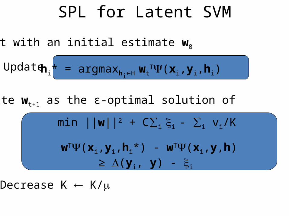
Start with an initial estimate w0
Update
min ||w||2 + C∑i i - ∑i vi/K
wT(xi,yi,hi*) - wT(xi,y,h)≥ (yi, y) - i
hi* = argmaxhiH wtT(xi,yi,hi)
Decrease K K/
SPL for Latent SVM
Update wt+1 as the ε-optimal solution of
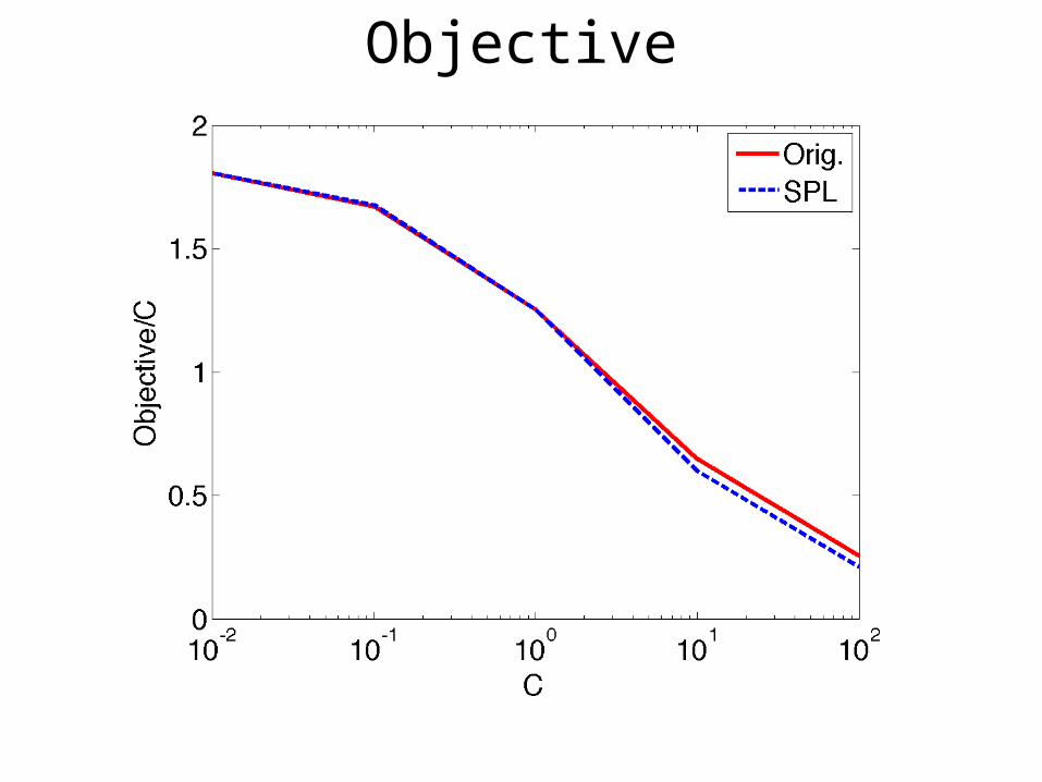
Objective
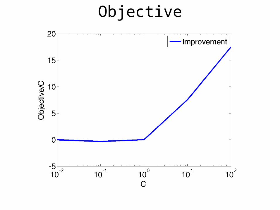
Objective
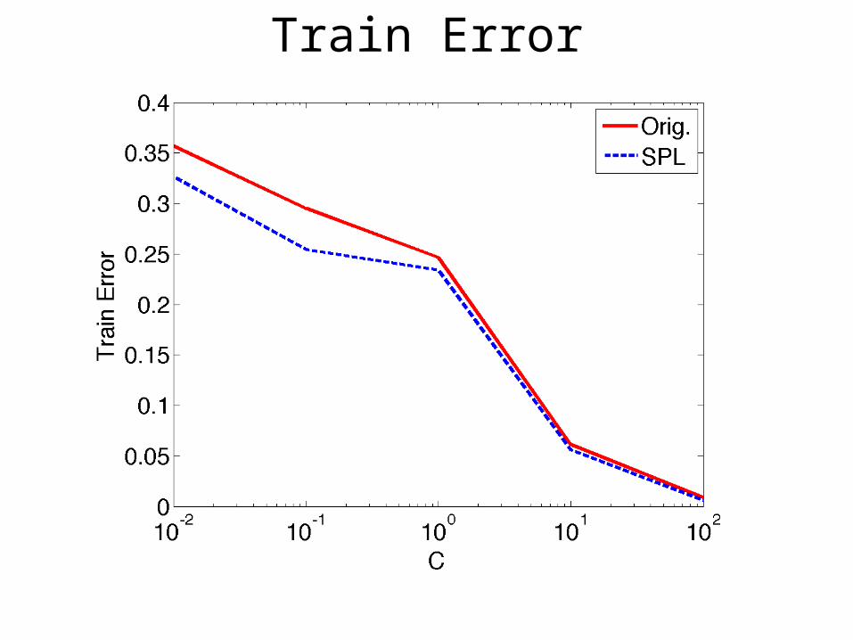
Train Error
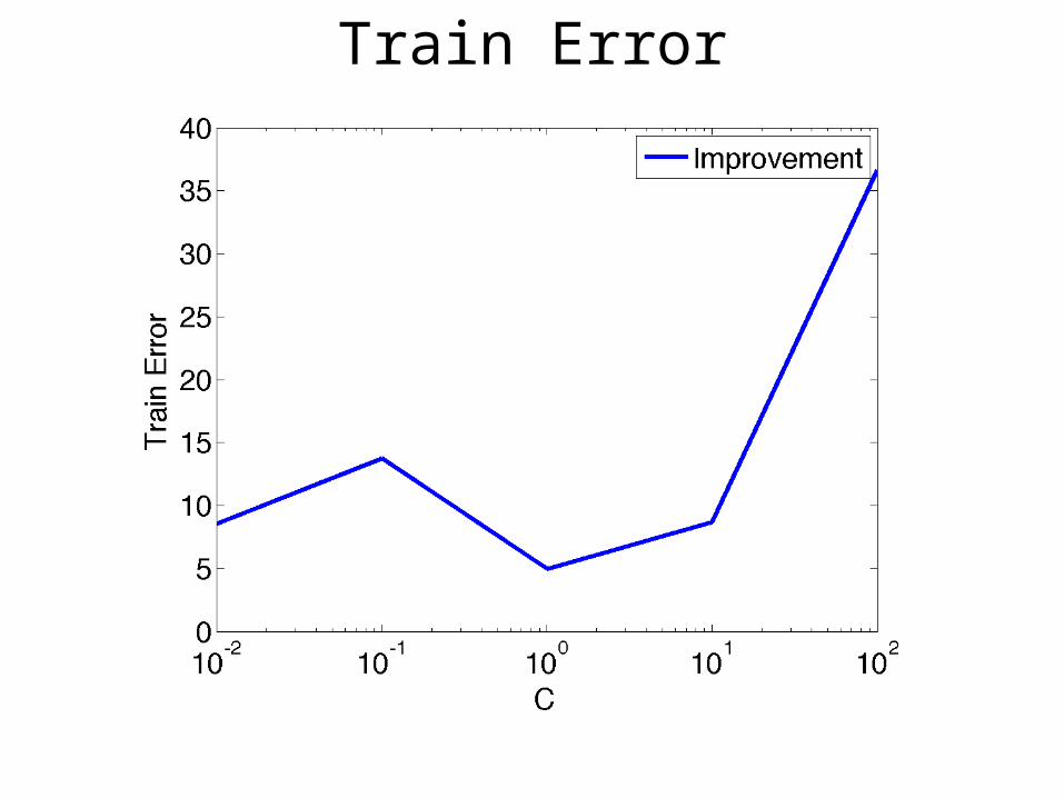
Train Error
Test Error
Test Error
Time
Time
• Latent SVM
• Optimization
• Practice– Annealing the Tolerance– Annealing the Regularization– Self-Paced Learning– Choice of Loss Function
• Extensions
Outline – Annotation Mismatch
Behl, Jawahar and Kumar, In Preparation
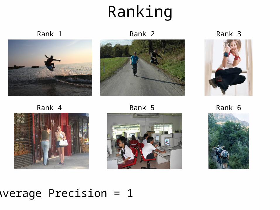
RankingRank 1 Rank 2 Rank 3
Rank 4 Rank 5 Rank 6
Average Precision = 1
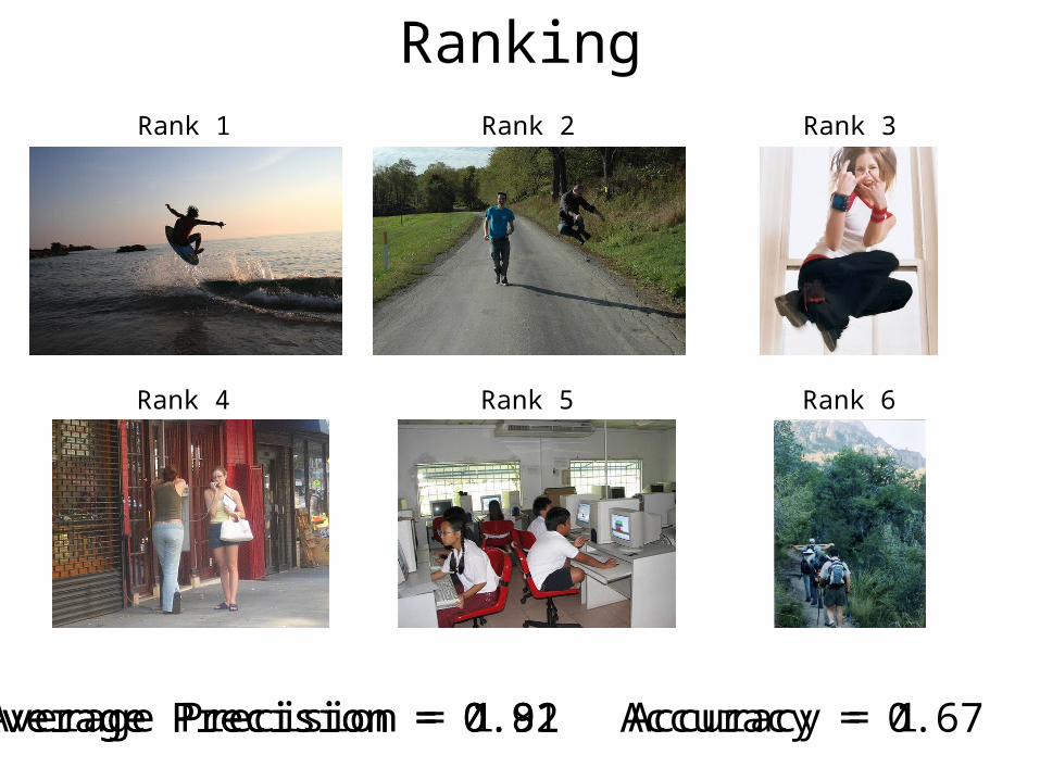
RankingRank 1 Rank 2 Rank 3
Rank 4 Rank 5 Rank 6
Average Precision = 1 Accuracy = 1Average Precision = 0.92 Accuracy = 0.67Average Precision = 0.81
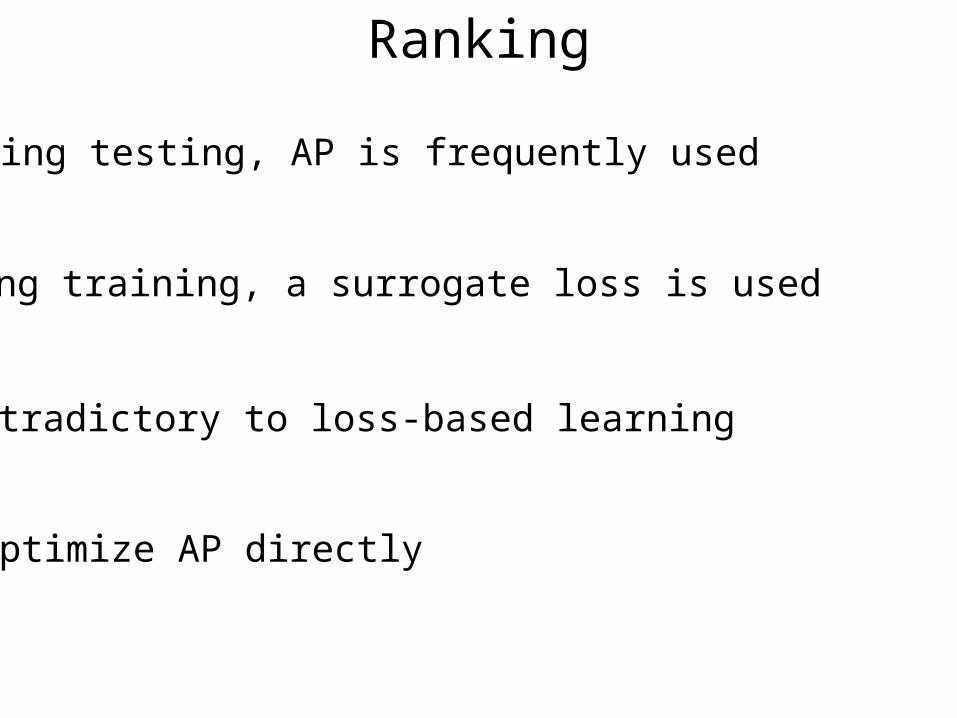
Ranking
During testing, AP is frequently used
During training, a surrogate loss is used
Contradictory to loss-based learning
Optimize AP directly
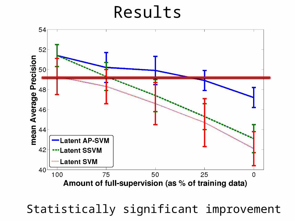
Results
Statistically significant improvement
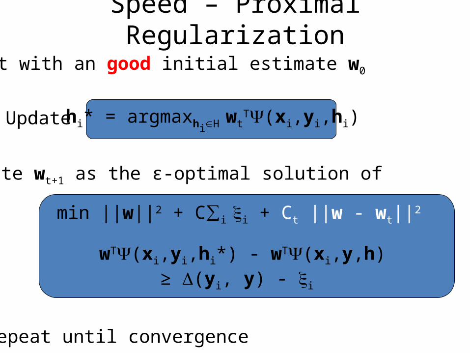
Speed – Proximal Regularization
Start with an good initial estimate w0
Update
Update wt+1 as the ε-optimal solution of
min ||w||2 + C∑i i + Ct ||w - wt||2
wT(xi,yi,hi*) - wT(xi,y,h)≥ (yi, y) - i
hi* = argmaxhiH wtT(xi,yi,hi)
Repeat until convergence
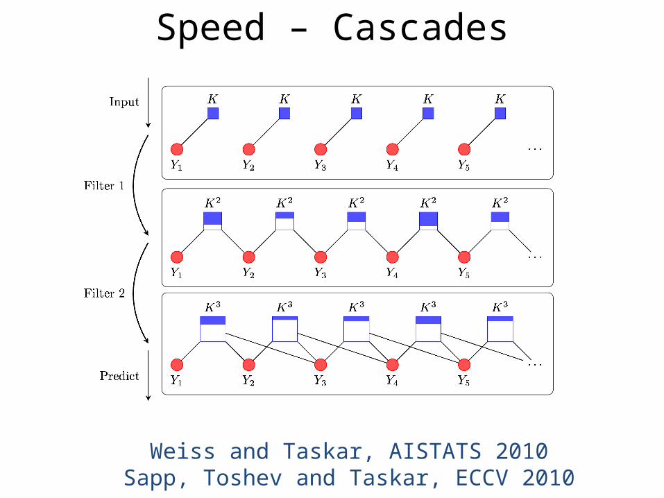
Speed – Cascades
Weiss and Taskar, AISTATS 2010Sapp, Toshev and Taskar, ECCV 2010
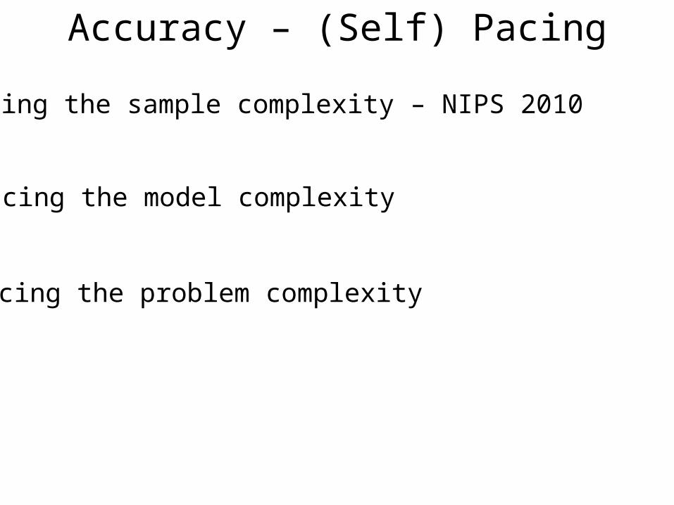
Accuracy – (Self) Pacing
Pacing the sample complexity – NIPS 2010
Pacing the model complexity
Pacing the problem complexity
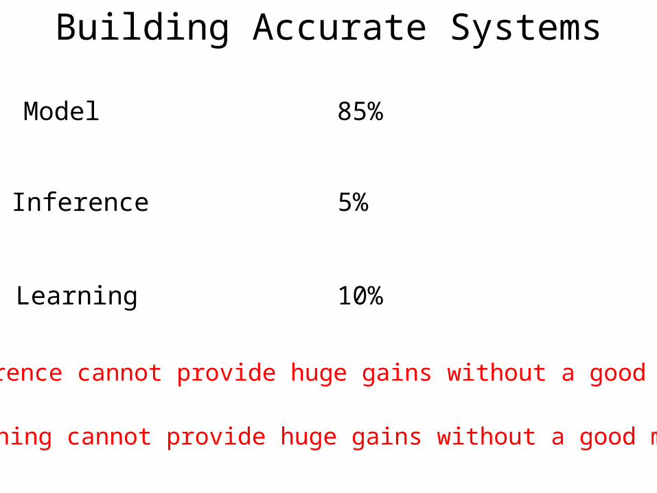
Building Accurate Systems
Model
Inference
Learning
85%
5%
10%
Learning cannot provide huge gains without a good model
Inference cannot provide huge gains without a good model
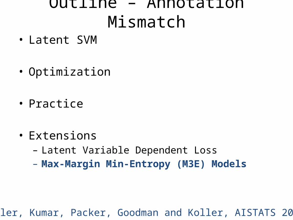
• Latent SVM
• Optimization
• Practice
• Extensions– Latent Variable Dependent Loss– Max-Margin Min-Entropy Models
Outline – Annotation Mismatch
Yu and Joachims, ICML 2009
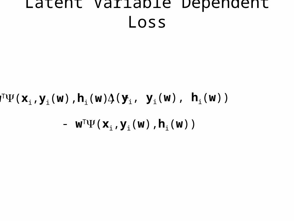
Latent Variable Dependent Loss
- wT(xi,yi(w),hi(w))
(yi, yi(w), hi(w))wT(xi,yi(w),hi(w)) +
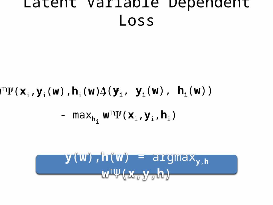
Latent Variable Dependent Loss
(yi, yi(w), hi(w))wT(xi,yi(w),hi(w)) +
- maxhi wT(xi,yi,hi)
y(w),h(w) = argmaxy,h wTΨ(x,y,h)
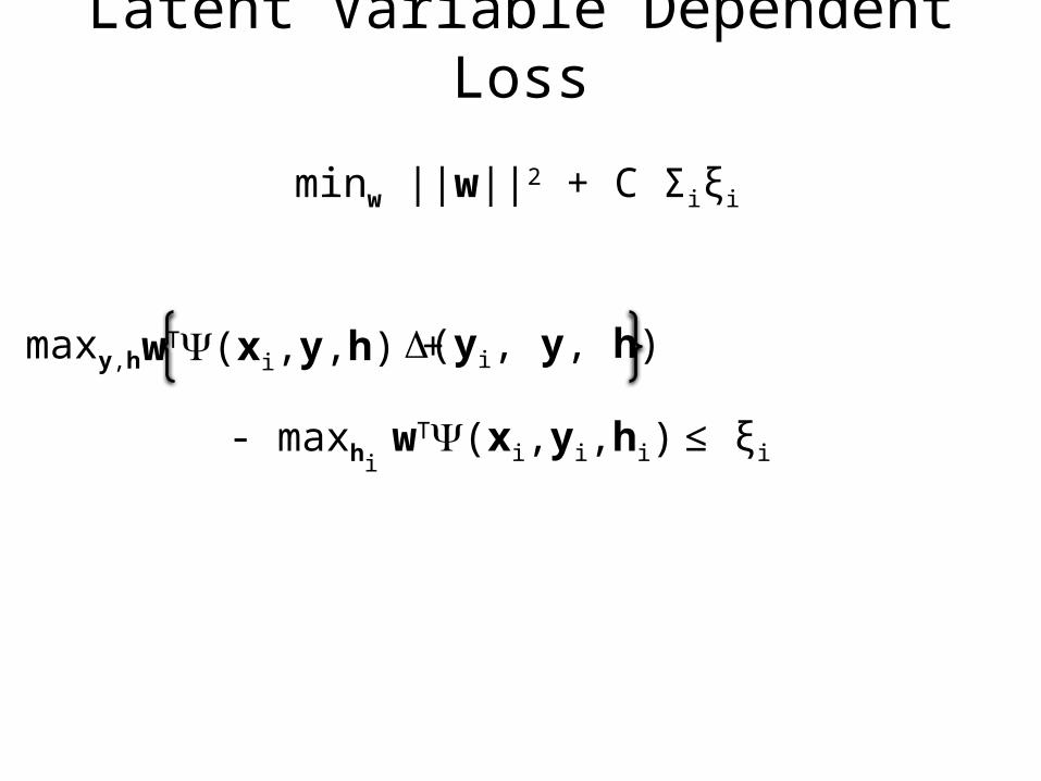
Latent Variable Dependent Loss
(yi, y, h)wT(xi,y,h) +maxy,h
- maxhi wT(xi,yi,hi) ≤ ξi
minw ||w||2 + C Σiξi
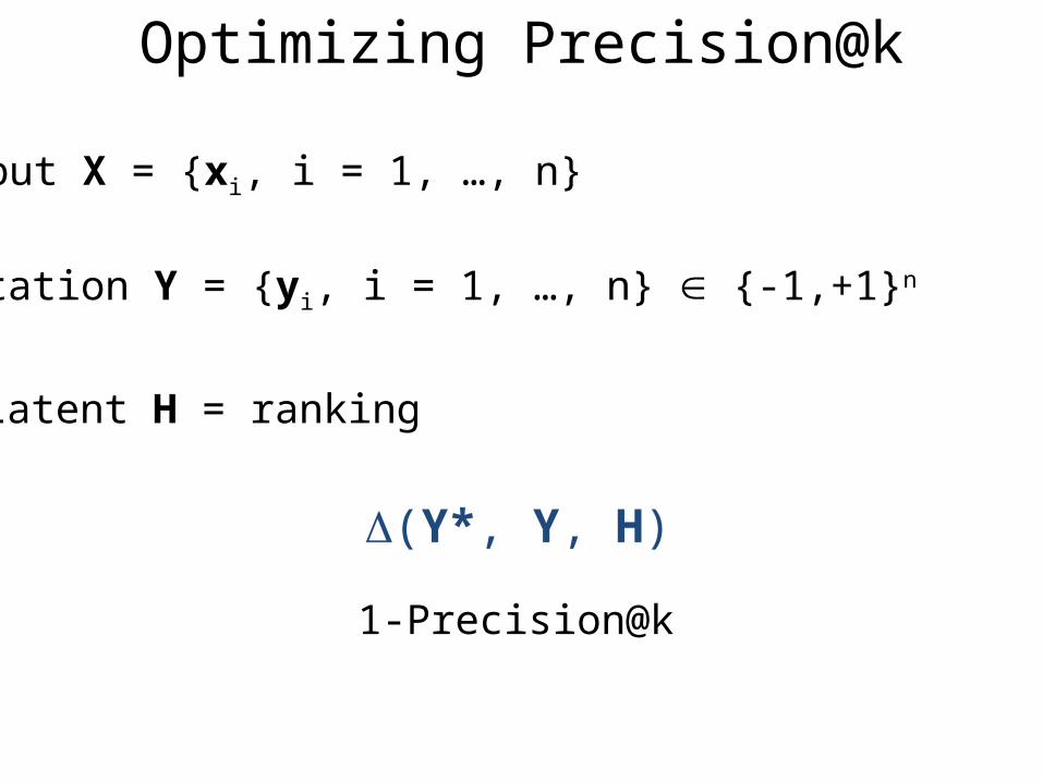
Optimizing Precision@k
Input X = {xi, i = 1, …, n}
Annotation Y = {yi, i = 1, …, n} {-1,+1}n
Latent H = ranking
(Y*, Y, H)
1-Precision@k
• Latent SVM
• Optimization
• Practice
• Extensions– Latent Variable Dependent Loss– Max-Margin Min-Entropy (M3E) Models
Outline – Annotation Mismatch
Miller, Kumar, Packer, Goodman and Koller, AISTATS 2012
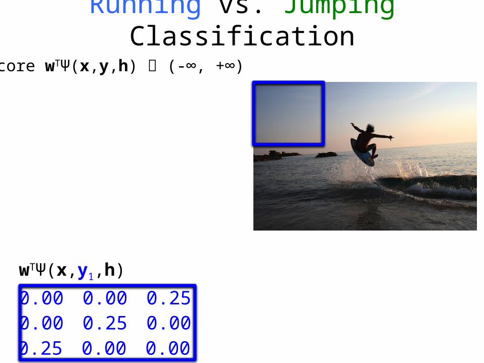
Running vs. Jumping Classification
0.00 0.00 0.250.00 0.25 0.000.25 0.00 0.00
Score wTΨ(x,y,h) (-∞, +∞)
wTΨ(x,y1,h)
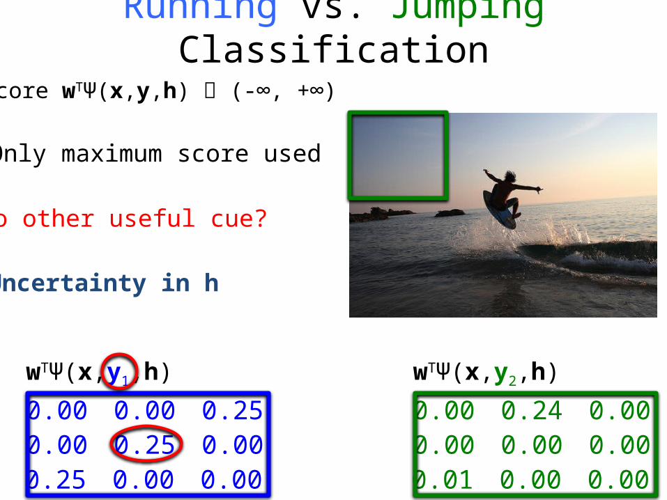
0.00 0.24 0.000.00 0.00 0.000.01 0.00 0.00
wTΨ(x,y2,h)
0.00 0.00 0.250.00 0.25 0.000.25 0.00 0.00
wTΨ(x,y1,h)
Only maximum score used
No other useful cue?
Score wTΨ(x,y,h) (-∞, +∞)
Uncertainty in h
Running vs. Jumping Classification
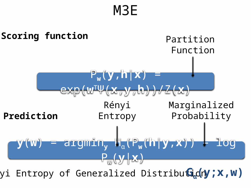
Scoring function
Pw(y,h|x) = exp(wTΨ(x,y,h))/Z(x)
Prediction
y(w) = argminy Hα(Pw(h|y,x)) – log Pw(y|x)
Partition Function
MarginalizedProbability
RényiEntropy
Rényi Entropy of Generalized Distribution Gα(y;x,w)
M3E
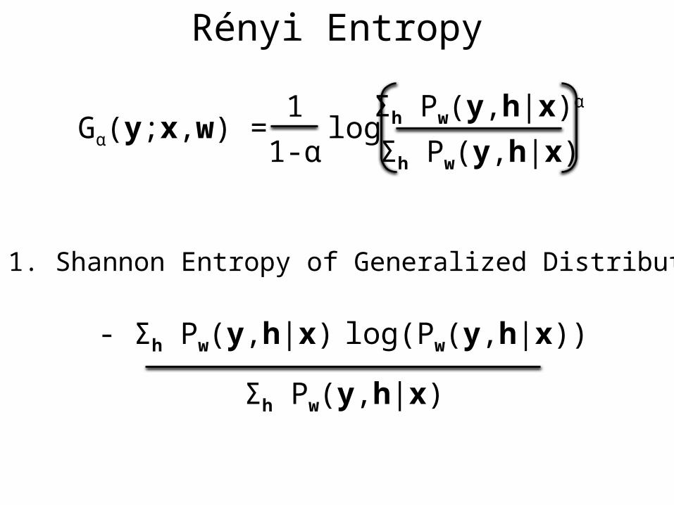
Gα(y;x,w) =1
1-αlog
Σh Pw(y,h|x)α
Σh Pw(y,h|x)
α = 1. Shannon Entropy of Generalized Distribution
- Σh Pw(y,h|x) log(Pw(y,h|x))
Σh Pw(y,h|x)
Rényi Entropy
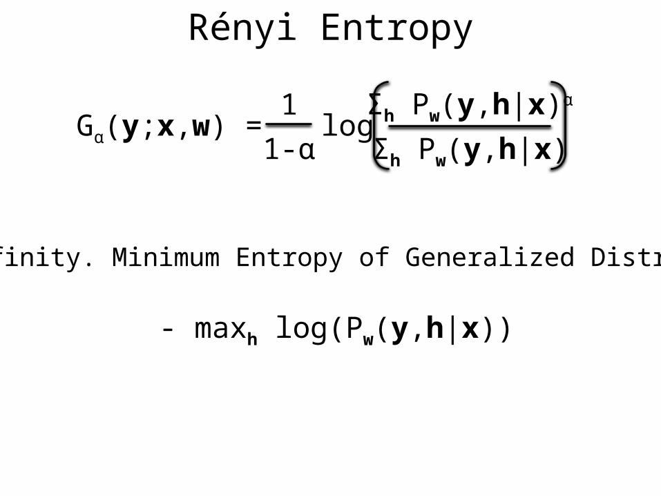
Gα(y;x,w) =1
1-αlog
Σh Pw(y,h|x)α
Σh Pw(y,h|x)
α = Infinity. Minimum Entropy of Generalized Distribution
- maxh log(Pw(y,h|x))
Rényi Entropy
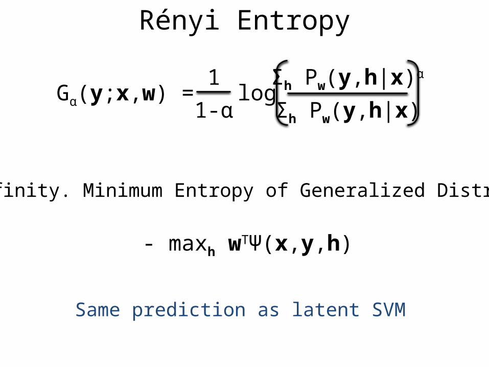
Gα(y;x,w) =1
1-αlog
Σh Pw(y,h|x)α
Σh Pw(y,h|x)
α = Infinity. Minimum Entropy of Generalized Distribution
- maxh wTΨ(x,y,h)
Same prediction as latent SVM
Rényi Entropy
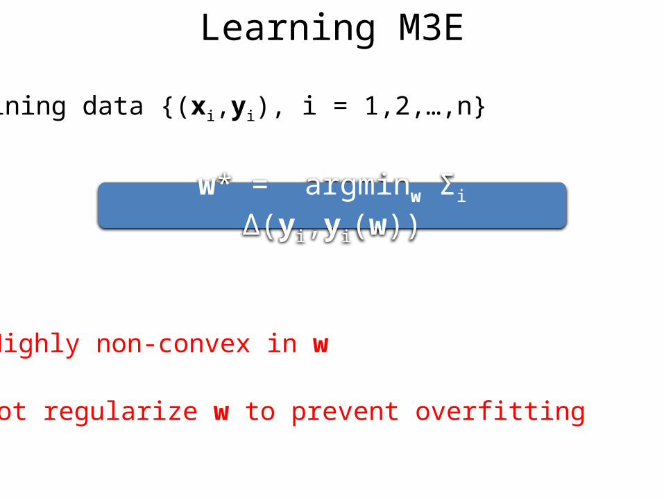
Training data {(xi,yi), i = 1,2,…,n}
Highly non-convex in w
Cannot regularize w to prevent overfitting
w* = argminw Σi Δ(yi,yi(w))
Learning M3E
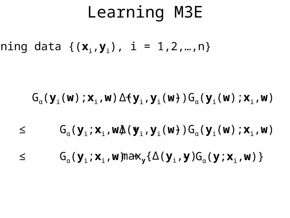
Δ(yi,yi(w))Gα(yi(w);xi,w) +
Training data {(xi,yi), i = 1,2,…,n}
- Gα(yi(w);xi,w)
Δ(yi,yi(w))≤ Gα(yi;xi,w) + - Gα(yi(w);xi,w)
maxy{Δ(yi,y)≤ Gα(yi;xi,w) + - Gα(y;xi,w)}
Learning M3E
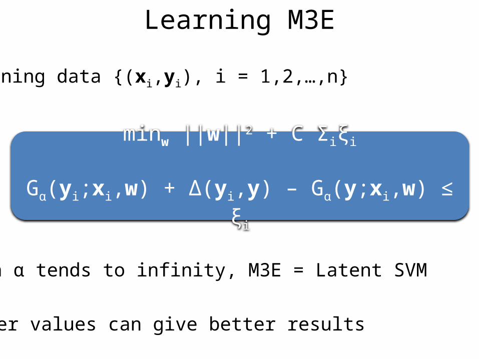
Training data {(xi,yi), i = 1,2,…,n}
minw ||w||2 + C Σiξi
Gα(yi;xi,w) + Δ(yi,y) – Gα(y;xi,w) ≤ ξi
When α tends to infinity, M3E = Latent SVM
Other values can give better results
Learning M3E
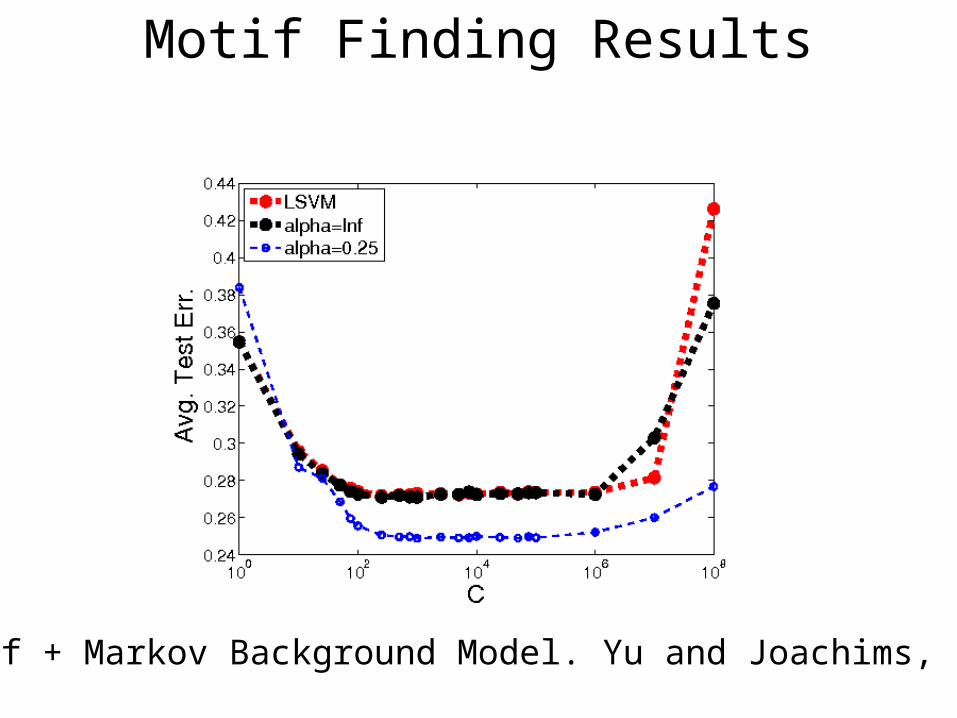
Motif + Markov Background Model. Yu and Joachims, 2009
Motif Finding Results

Part II
Output Mismatch
Input x
Annotation y
Latent h
x
y = “jumping”
h
Action Detection
Mismatch between output and available annotations
Exact value of latent variable is important
Desired output during test time is (y,h)
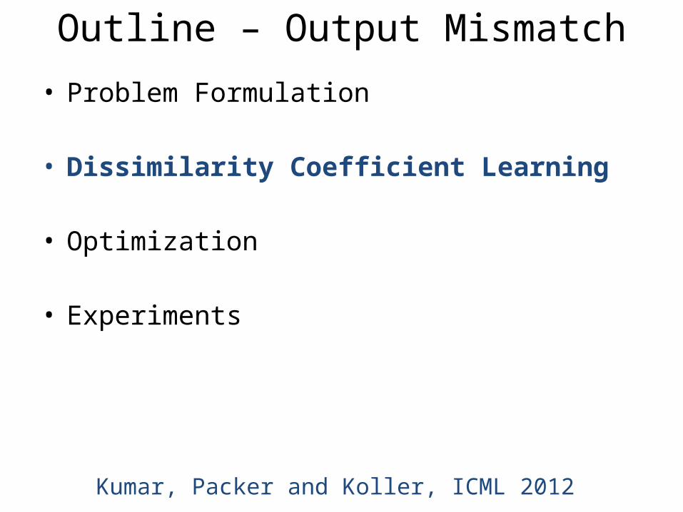
• Problem Formulation
• Dissimilarity Coefficient Learning
• Optimization
• Experiments
Outline – Output Mismatch
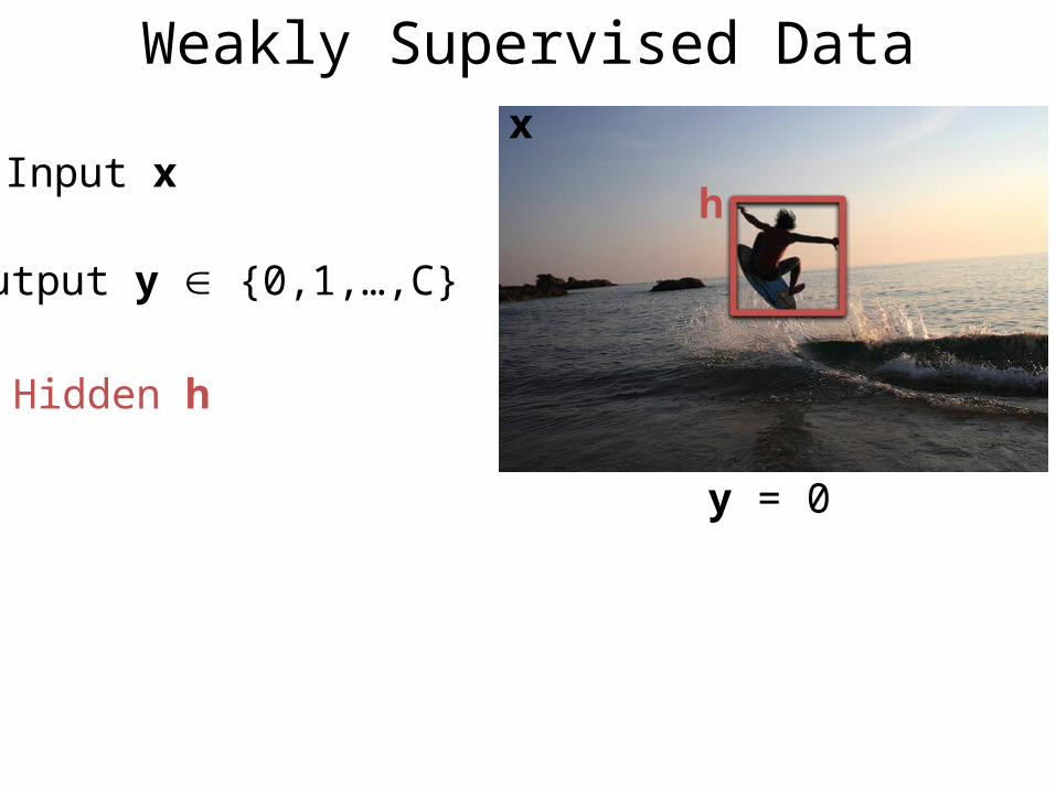
Weakly Supervised Data
Input x
Output y {0,1,…,C}
Hidden h
x
y = 0
h
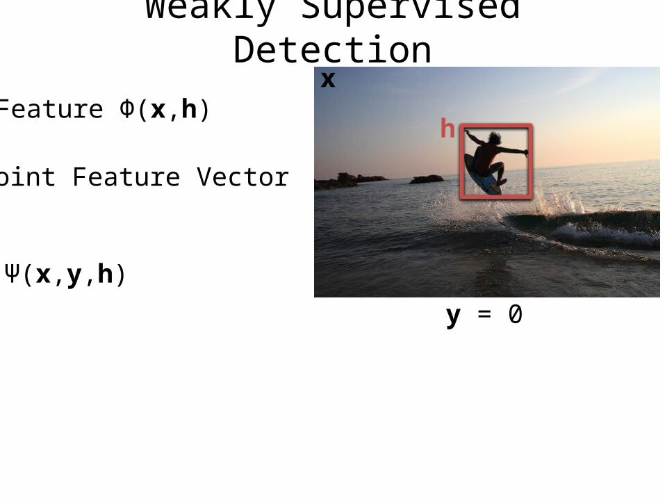
Weakly Supervised Detection
Feature Φ(x,h)
Joint Feature Vector
Ψ(x,y,h)
x
y = 0
h
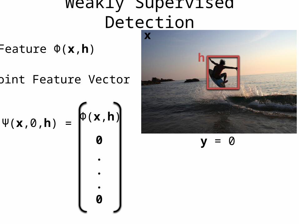
Weakly Supervised Detection
Feature Φ(x,h)
Joint Feature Vector
Ψ(x,0,h) Φ(x,h)
0
=
x
y = 0
h
0
.
.
.

Weakly Supervised Detection
Feature Φ(x,h)
Joint Feature Vector
Ψ(x,1,h) 0
Φ(x,h)
=
x
y = 0
h
0
.
.
.
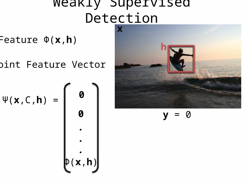
Weakly Supervised Detection
Feature Φ(x,h)
Joint Feature Vector
Ψ(x,C,h) 0
0
=
x
y = 0
h
Φ(x,h)
.
.
.
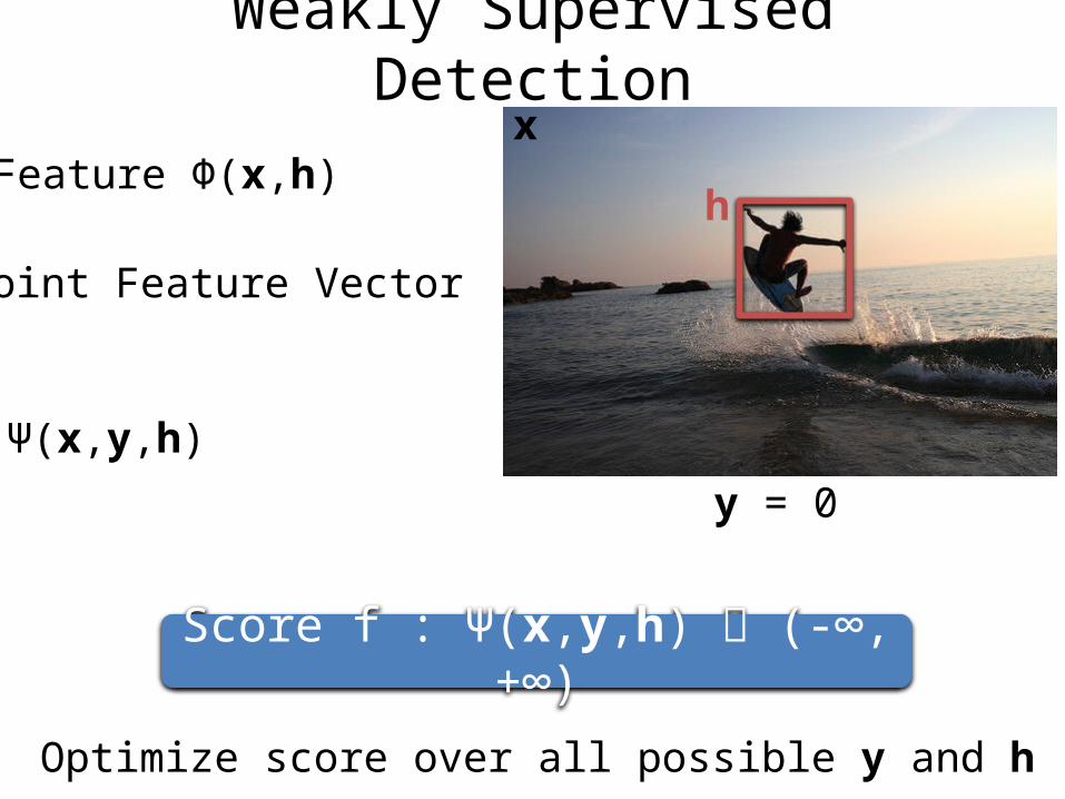
Weakly Supervised Detection
Feature Φ(x,h)
Joint Feature Vector
Ψ(x,y,h)
Score f : Ψ(x,y,h) (-∞, +∞)
Optimize score over all possible y and h
x
y = 0
h
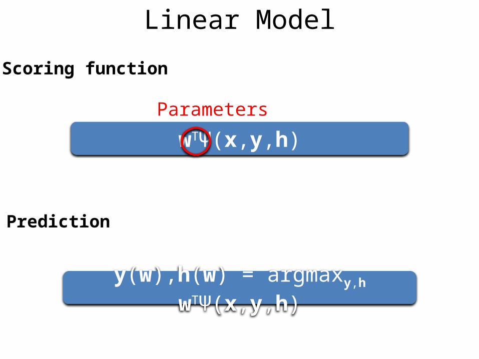
Scoring function
wTΨ(x,y,h)
Prediction
y(w),h(w) = argmaxy,h wTΨ(x,y,h)
Linear Model
Parameters
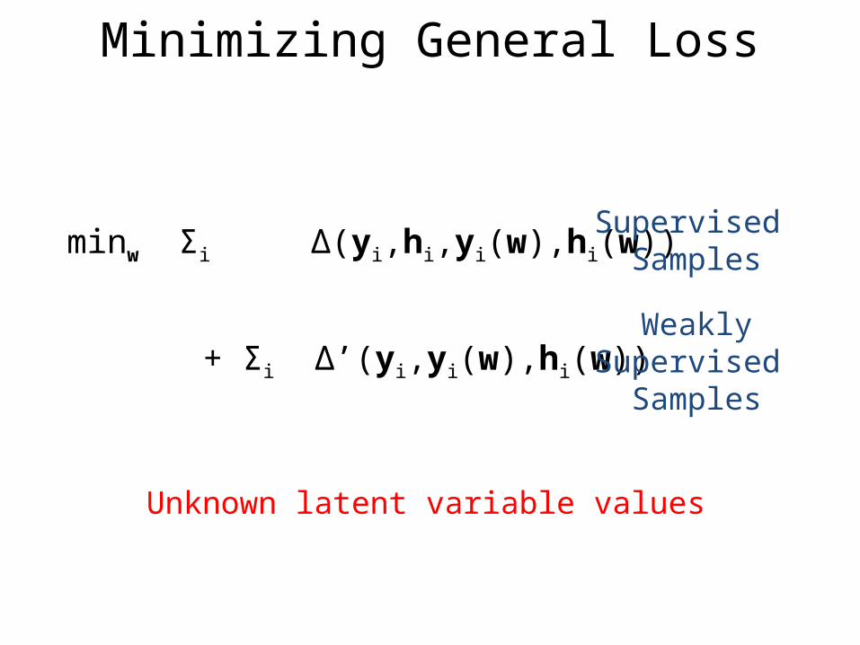
Minimizing General Loss
minw Σi Δ(yi,hi,yi(w),hi(w))
Unknown latent variable values
Supervised Samples
+ Σi Δ’(yi,yi(w),hi(w))Weakly
Supervised Samples
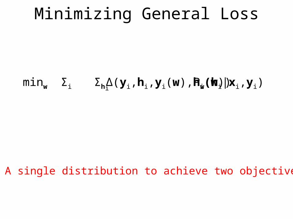
Minimizing General Loss
minw Σi Δ(yi,hi,yi(w),hi(w))
A single distribution to achieve two objectives
Pw(hi|xi,yi)Σhi
• Problem Formulation
• Dissimilarity Coefficient Learning
• Optimization
• Experiments
Outline – Output Mismatch
Kumar, Packer and Koller, ICML 2012
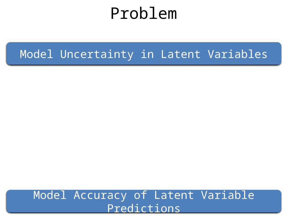
Problem
Model Uncertainty in Latent Variables
Model Accuracy of Latent Variable Predictions
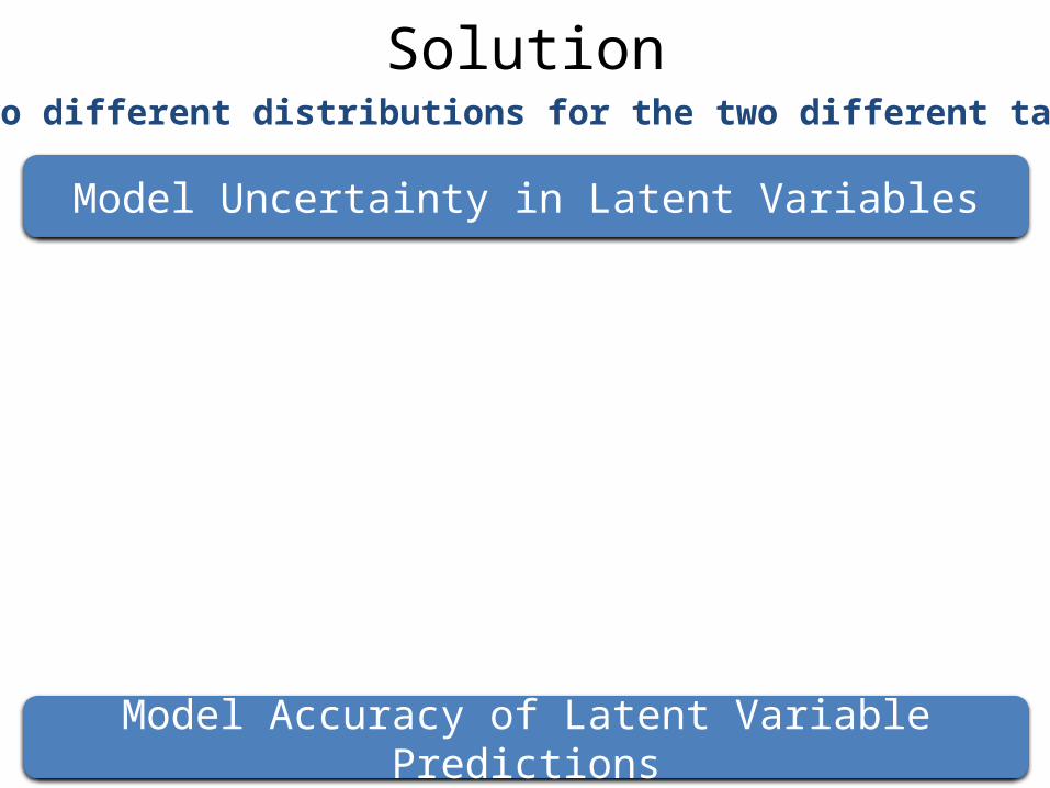
Solution
Model Uncertainty in Latent Variables
Model Accuracy of Latent Variable Predictions
Use two different distributions for the two different tasks
Solution
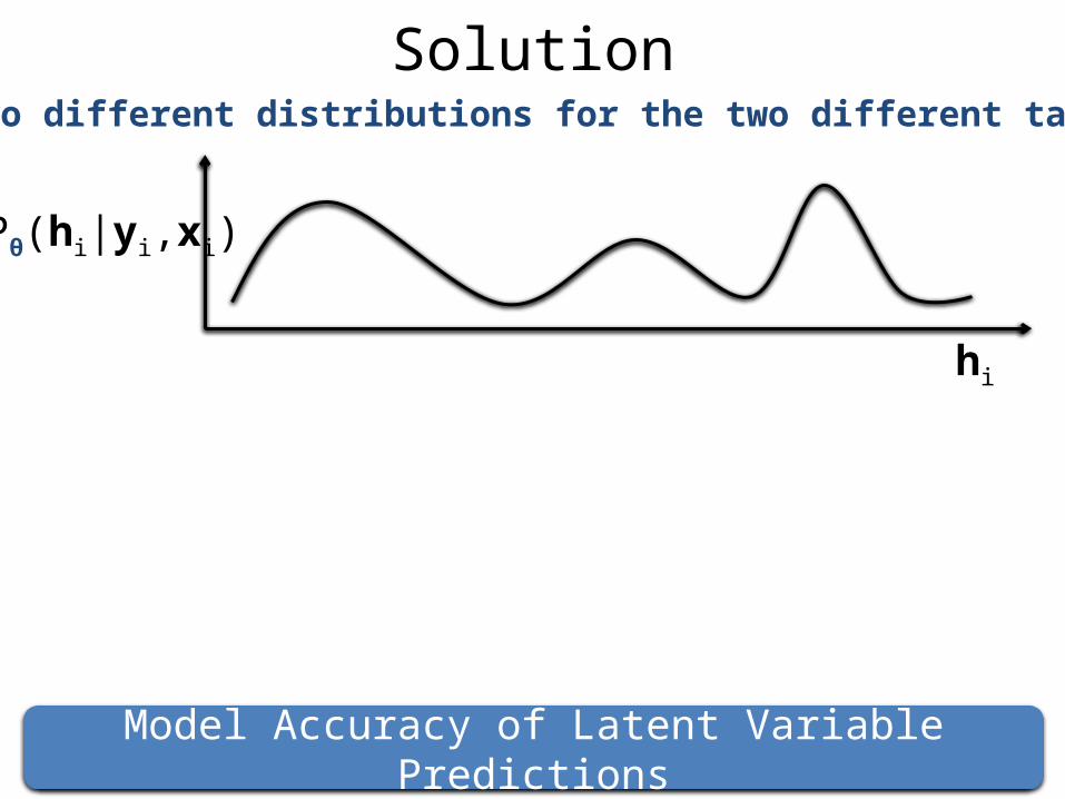
Model Accuracy of Latent Variable Predictions
Use two different distributions for the two different tasks
Pθ(hi|yi,xi)
hi
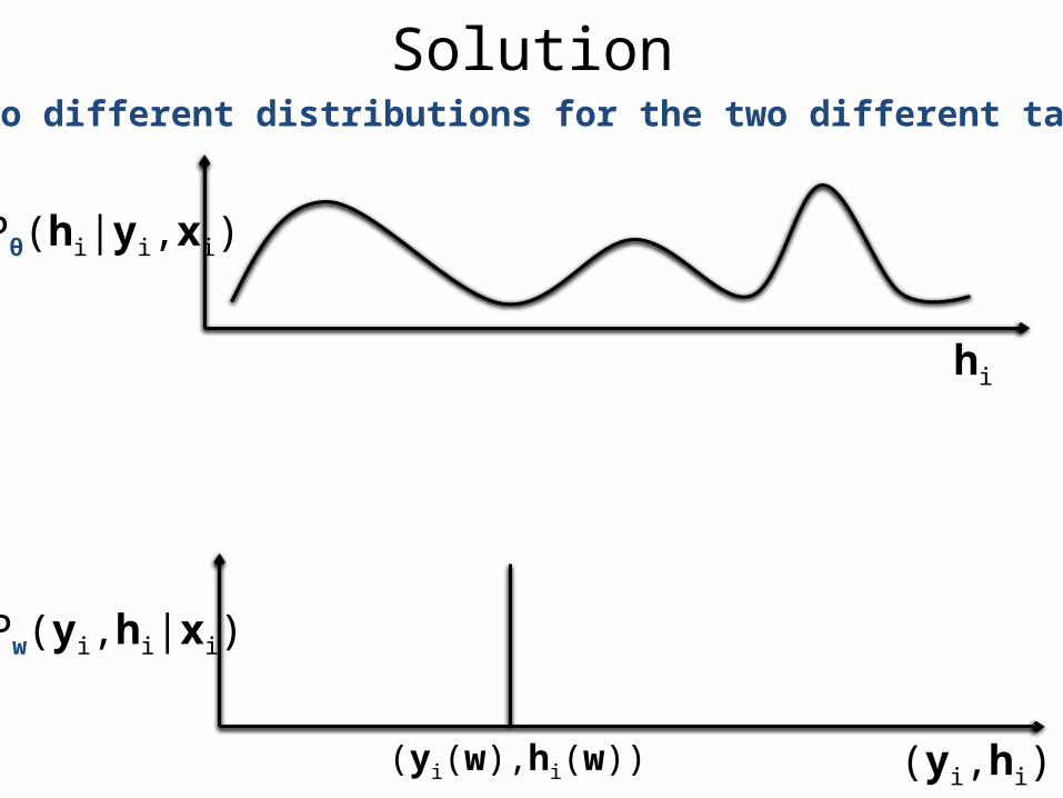
SolutionUse two different distributions for the two different tasks
hi
Pw(yi,hi|xi)
(yi,hi)(yi(w),hi(w))
Pθ(hi|yi,xi)
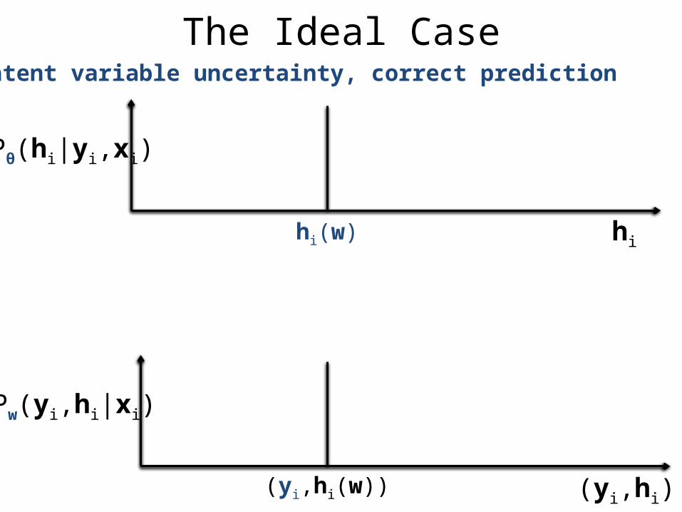
The Ideal CaseNo latent variable uncertainty, correct prediction
hi
Pw(yi,hi|xi)
(yi,hi)(yi,hi(w))
Pθ(hi|yi,xi)
hi(w)
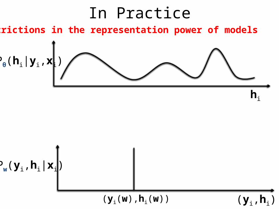
In PracticeRestrictions in the representation power of models
hi
Pw(yi,hi|xi)
(yi,hi)(yi(w),hi(w))
Pθ(hi|yi,xi)
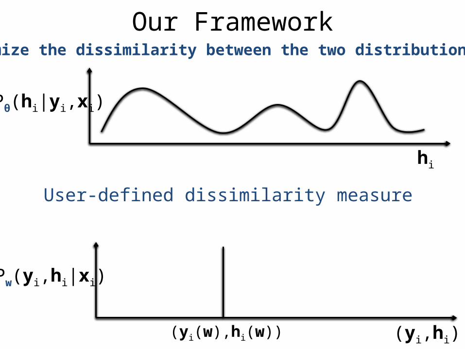
Our FrameworkMinimize the dissimilarity between the two distributions
hi
Pw(yi,hi|xi)
(yi,hi)(yi(w),hi(w))
Pθ(hi|yi,xi)
User-defined dissimilarity measure
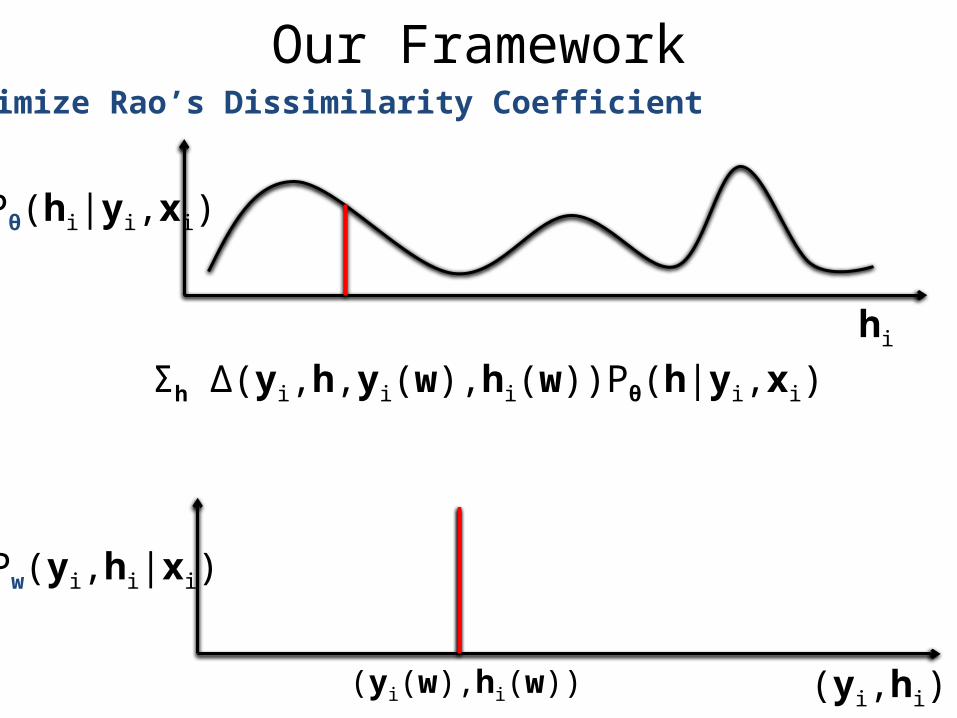
Our FrameworkMinimize Rao’s Dissimilarity Coefficient
hi
Pw(yi,hi|xi)
(yi,hi)(yi(w),hi(w))
Pθ(hi|yi,xi)
Σh Δ(yi,h,yi(w),hi(w))Pθ(h|yi,xi)
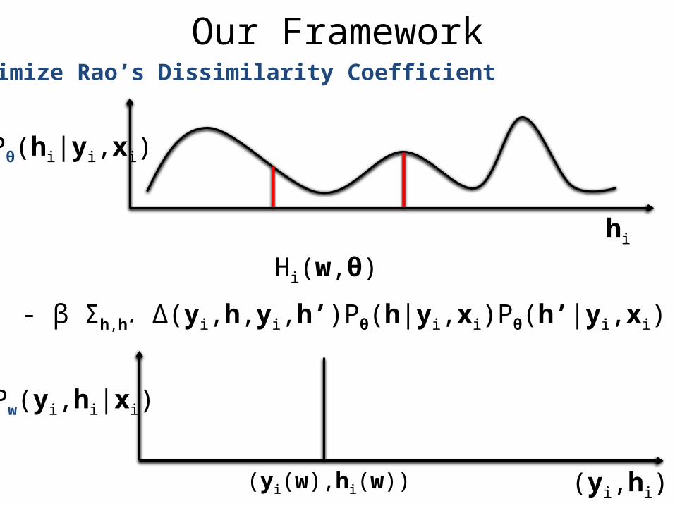
Our FrameworkMinimize Rao’s Dissimilarity Coefficient
hi
Pw(yi,hi|xi)
(yi,hi)(yi(w),hi(w))
Pθ(hi|yi,xi)
- β Σh,h’ Δ(yi,h,yi,h’)Pθ(h|yi,xi)Pθ(h’|yi,xi)
Hi(w,θ)
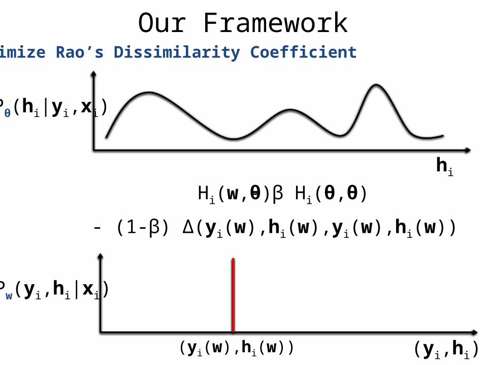
Our FrameworkMinimize Rao’s Dissimilarity Coefficient
hi
Pw(yi,hi|xi)
(yi,hi)(yi(w),hi(w))
Pθ(hi|yi,xi)
- (1-β) Δ(yi(w),hi(w),yi(w),hi(w))
- β Hi(θ,θ)Hi(w,θ)
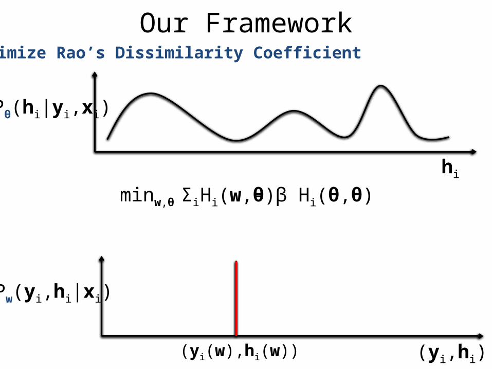
Our FrameworkMinimize Rao’s Dissimilarity Coefficient
hi
Pw(yi,hi|xi)
(yi,hi)(yi(w),hi(w))
Pθ(hi|yi,xi)
- β Hi(θ,θ)Hi(w,θ)minw,θ Σi
• Problem Formulation
• Dissimilarity Coefficient Learning
• Optimization
• Experiments
Outline – Output Mismatch
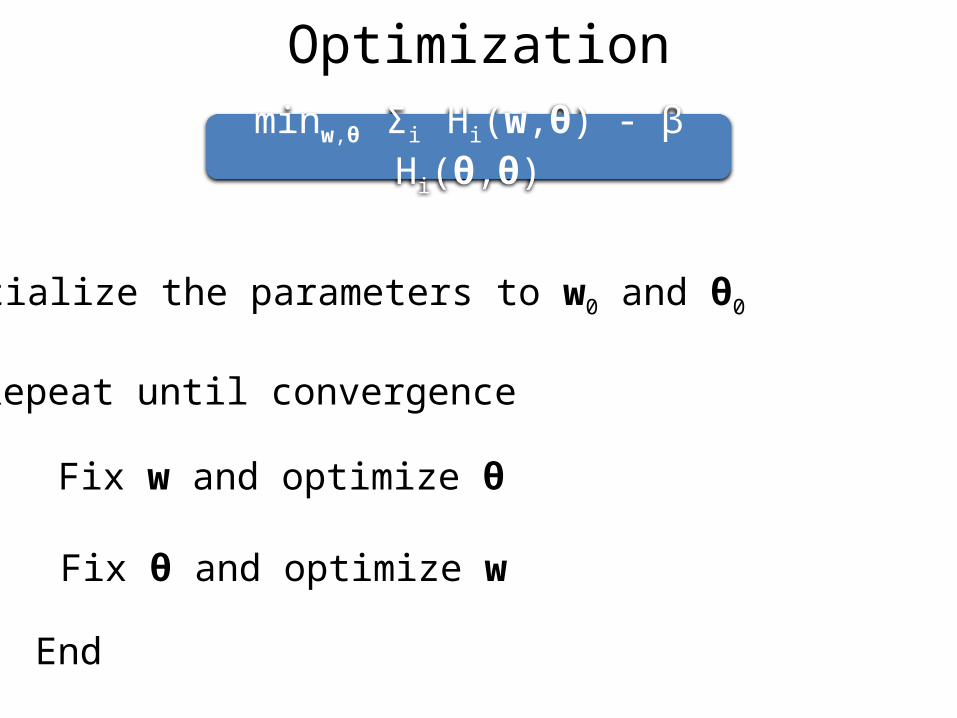
Optimization
minw,θ Σi Hi(w,θ) - β Hi(θ,θ)
Initialize the parameters to w0 and θ0
Repeat until convergence
End
Fix w and optimize θ
Fix θ and optimize w
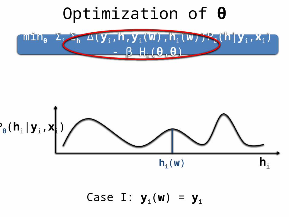
Optimization of θ
minθ Σi Σh Δ(yi,h,yi(w),hi(w))Pθ(h|yi,xi) - β Hi(θ,θ)
hi
Pθ(hi|yi,xi)
Case I: yi(w) = yi
hi(w)
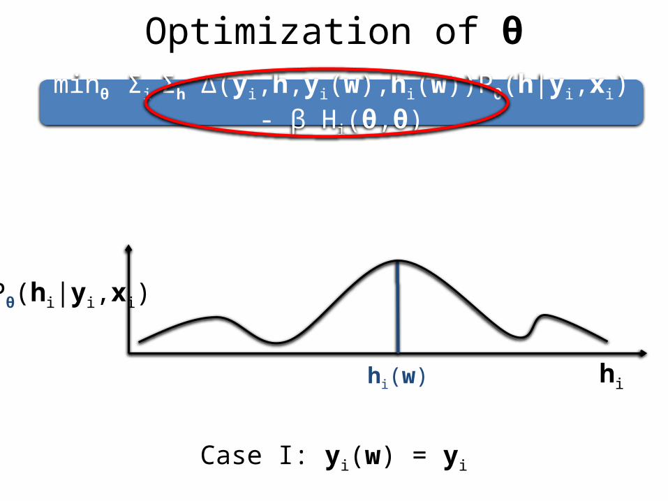
Optimization of θ
minθ Σi Σh Δ(yi,h,yi(w),hi(w))Pθ(h|yi,xi) - β Hi(θ,θ)
hi
Pθ(hi|yi,xi)
Case I: yi(w) = yi
hi(w)
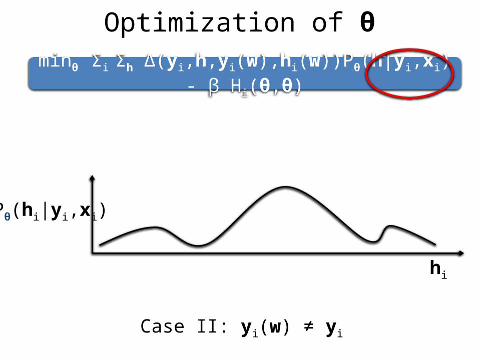
Optimization of θ
minθ Σi Σh Δ(yi,h,yi(w),hi(w))Pθ(h|yi,xi) - β Hi(θ,θ)
hi
Pθ(hi|yi,xi)
Case II: yi(w) ≠ yi
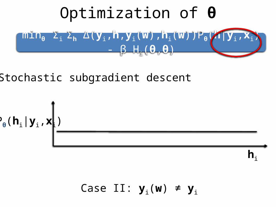
Optimization of θ
minθ Σi Σh Δ(yi,h,yi(w),hi(w))Pθ(h|yi,xi) - β Hi(θ,θ)
hi
Pθ(hi|yi,xi)
Case II: yi(w) ≠ yi
Stochastic subgradient descent
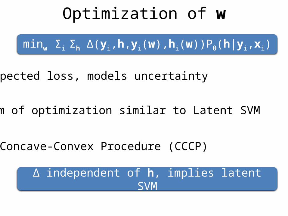
Optimization of w
minw Σi Σh Δ(yi,h,yi(w),hi(w))Pθ(h|yi,xi)
Expected loss, models uncertainty
Form of optimization similar to Latent SVM
Δ independent of h, implies latent SVM
Concave-Convex Procedure (CCCP)
• Problem Formulation
• Dissimilarity Coefficient Learning
• Optimization
• Experiments
Outline – Output Mismatch
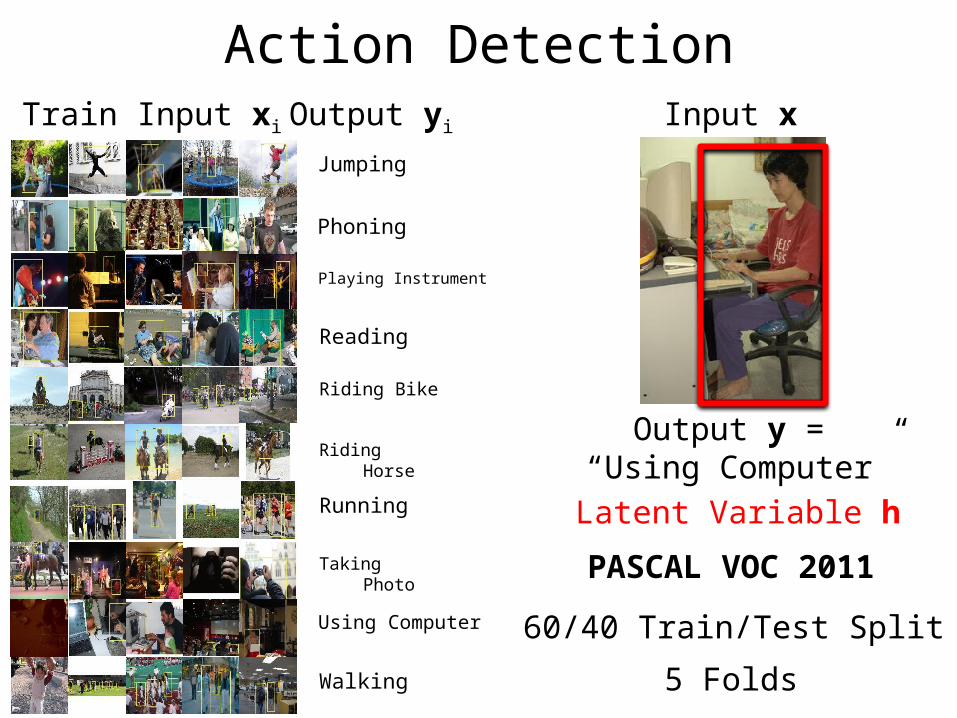
Action DetectionInput x
Output y = “Using Computer”
Latent Variable h
PASCAL VOC 2011
60/40 Train/Test Split
5 Folds
Jumping
Phoning
Playing Instrument
Reading
Riding Bike
Riding Horse
Running
Taking Photo
Using Computer
Walking
Train Input xi Output yi
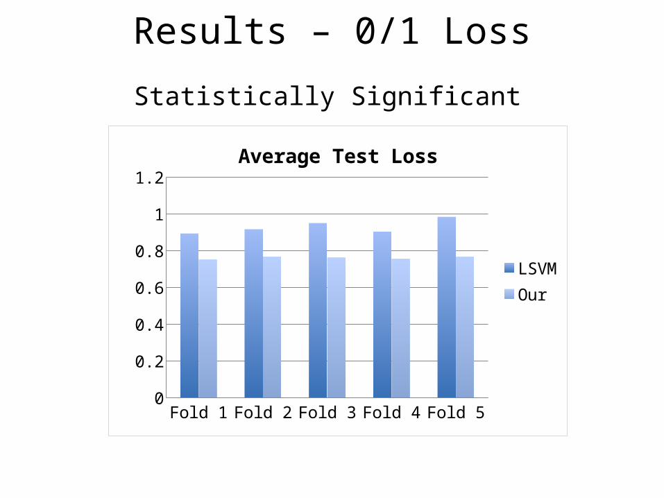
Results – 0/1 Loss
Fold 1 Fold 2 Fold 3 Fold 4 Fold 50
0.2
0.4
0.6
0.8
1
1.2
Average Test Loss
LSVMOur
Statistically Significant
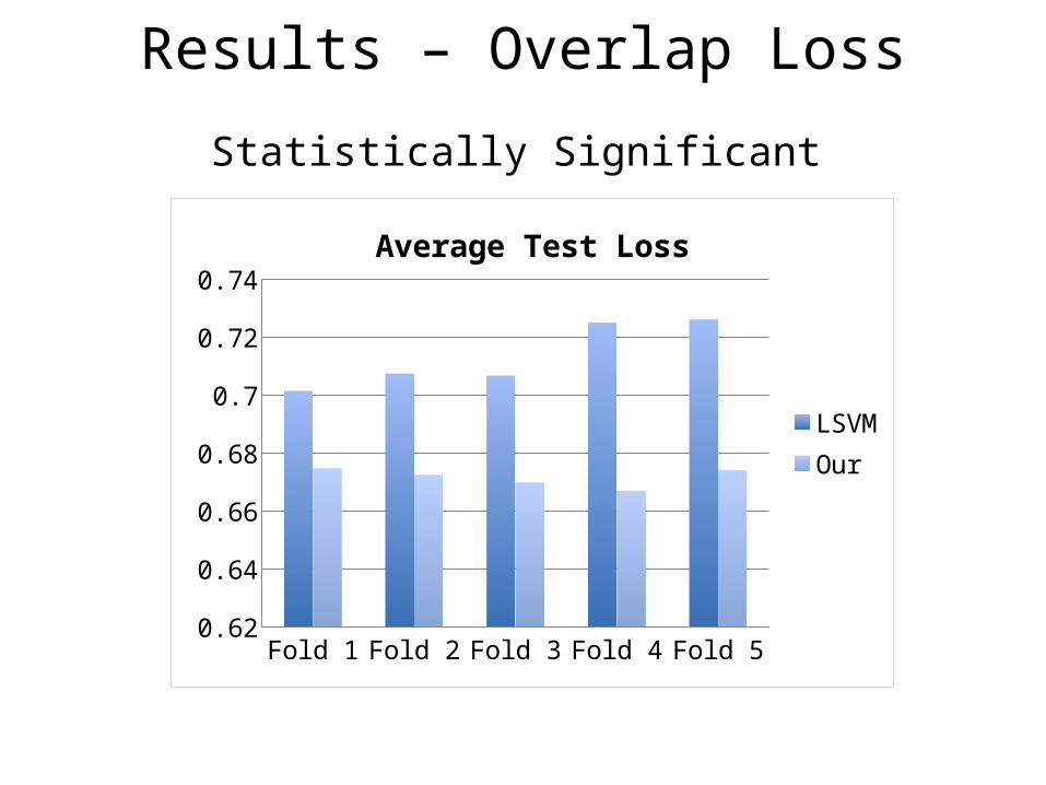
Results – Overlap Loss
Fold 1 Fold 2 Fold 3 Fold 4 Fold 50.62
0.64
0.66
0.68
0.7
0.72
0.74
Average Test Loss
LSVMOur
Statistically Significant

Questions?
http://www.centrale-ponts.fr/personnel/pawan