Low-Complexity Separable Beamformers for Massive Antenna

IET Research Journals

Research Article

Low-Complexity Separable Beamformers forMassive Antenna Array Systems

ISSN 1751-8644doi: 0000000000www.ietdl.org

Lucas N. Ribeiro1 , André L. F. de Almeida1, Josef A. Nossek1,2, João César M. Mota1

1Wireless Telecommunications Research Group, Federal University of Ceará, Fortaleza, Brazil.2Department of Electrical and Computer Engineering, Technical University Munich, Munich, Germany.

E-mail: [email protected]

Abstract:Future cellular systems will likely employ massive bi-dimensional arrays to improve performance by large array gain and moreaccurate spatial filtering, motivating the design of low-complexity signal processing methods. We propose optimising a Kronecker-separable beamforming filter that takes advantage of the bi-dimensional array geometry to reduce computational costs. TheKronecker factors are obtained using two strategies: alternating optimisation, and sub-array minimum mean square error beam-forming with Tikhonov regularization. According to the simulation results, the proposed methods are computationally efficient butcome with source recovery degradation, which becomes negligible when the sources are sufficiently separated in space.

1 Introduction

The number of wireless connected devices has been growing sig-nificantly, bringing new challenges to engineers. Future mobilecommunications systems, for example, are expected to provide veryhigh throughput to several mobile terminals. In order to boost sys-tem capacity, new transceiver and network architectures are underinvestigation. Massive multiple-input-multiple-output (MIMO) tech-nology, which consists of employing a large number of antennaelements at the base station (BS) to serve many multi-antennausers, is expected to yield significant spectral efficiency improve-ment [1, 2]. Such massive systems should be implemented usingplanar arrays in order to reduce the array’s physical dimensionsand to perform elevation and azimuth beamforming. This imple-mentation, known as full-dimension MIMO (FD-MIMO), allowsfor better interference mitigation and has already been incorporatedinto 3GPP standards [3]. These technologies pose new engineeringchallenges concerning computational and energy efficiency [4], call-ing for research efforts to design computationally efficient signalprocessing methods for high-dimensional systems. ∗

The high computational complexity of multidimensional filter-ing systems is not a new problem, though, and the first attemptsto tackle this problem can be traced back to some decades ago.For instance, the authors in [5] proposed a multi-stage represen-tation for bi-dimensional filters based on the coefficient matrixeigendecomposition, yielding computer storage and speed savings.However, computing the eigendecomposition of high-dimensionalobservations is expensive in general. More recent works have beeninterested in exploiting the algebraic structure present in someproblems to reduce computational costs and to improve system per-formance. The authors in [6] introduced tensor-based blind sourceseparation methods which reduce the number of parameters to beestimated by exploiting the structure of low-rank signals. Such prop-erty implies that signals can be well approximated by a finite sumof low-dimensional Kronecker products. Although this representa-tion simplifies the parameter estimation problem, signal accuracyis degraded. Kronecker separability has also been exploited in [7–9] to increase the convergence rate of adaptive algorithms. Gradient

∗This paper is a preprint of a paper accepted by IET Signal Processing and

is subject to Institution of Engineering and Technology Copyright. When

the final version is published, the copy of record will be available at the

IET Digital Library

descent-based solutions were presented in [7, 8] to identify second-order Kronecker separable systems, which can be useful to modeltelephone hybrid causing electrical echoes. In [9], the authors showthat Volterra systems with separable kernels can be expressed interms of Kronecker products. In [10], we introduce a supervisedsystem identification method to identify third-order Kronecker sep-arable impulse responses based on alternating optimisation. Theproposed identification method is applied to identify the telephonehybrid-like impulse response of [7]. Simulation results indicate thatthe proposed method exhibits better accuracy than the classicalWiener filter solution. In [11], the method of [10] is extended to copewith low-rank Kronecker separable systems, allowing for the identi-fication of more intricate acoustic responses. In [12], fast recursiveleast squares methods for identifying second-order Kronecker sep-arable (bilinear) systems are presented. Analytical and simulationresults confirm the low computational costs and the identificationperformance of the proposed bilinear methods.

It is well-known that the spatial signature of planar arrays canbe decomposed along its two dimensions [13]. Based on this prop-erty, beamforming techniques have been proposed. The authorsin [14] obtained a low-complexity two-dimensional MIMO precod-ing scheme by exploiting the Kronecker structure in the steeringvectors of rectangular arrays. Therein, the proposed separable zero-forcing (ZF) precoder is presented based on the small angular spreadat the elevation domain assumption, which enables algebraic sep-aration of the azimuth and elevation domains by filtering. Resultsshow that when this assumption is satisfied, the proposed separa-ble ZF filter exhibits acceptable performance. However, in morerealistic scenarios, this assumption is seldom met, and the perfor-mance of the separable ZF filter is severely degraded. In [15], aclever hybrid analogue/digital beamforming method based on theKronecker product is proposed for multi-cell multi-user MIMO sys-tems. The analogue beamformers are designed exploiting the mixedproduct property of the Kronecker product to null inter-cell interfer-ence and to enhance the desired signal power. In [16], the authorsinvestigate the performance of a tensor global sidelobe canceller(GSC). Simulation results suggest that this tensor-based beamformerrequires fewer snapshots than the classical GSC filter to achievethe desired performance. A tensor minimum variance distortionlessresponse beamformer has been introduced in [17] for polarizationsensitive arrays. In [18], we express the received signal vector ofa massive MIMO system equipped with a planar array using mul-tilinear (tensor) algebra. From this model, we derived a two-steplow-complexity equaliser which exploits each signal dimension,

IET Research Journals, pp. 1–10c© The Institution of Engineering and Technology 2015 1

similar to [14]. It basically consists of sub-array ZF beamform-ing followed by a low-dimensional minimum mean square error(MMSE) equaliser.

In this present work, we propose novel beamforming techniqueswhich exploit the array separability to reduce their computationalcosts. Our methods are based on the classical MMSE beamformer,also known as Wiener filter [19]. This filter may be computationallyimpractical due to the inversion of a possibly very large covari-ance matrix. The matrix inversion lemma [20] can be applied to theMMSE beamformer when the signal statistics are perfectly known,however, in practice, this seldom happens. As alternatives to the clas-sical MMSE solution, we propose methods which aim at optimisinga beamforming filter with Kronecker structure, i.e., the coefficientsvector admits a Kronecker factorization. Thus, instead of optimis-ing a large beamforming vector, we propose designing two relativelysmall beamforming vectors corresponding to the Kronecker factors.We present two strategies to design a Kronecker separable filter. Inthe first strategy, the mean square error (MSE) function is minimisedby means of alternating optimisation. This strategy was first intro-duced in [21], where the beamforming filter is obtained using sampleestimates of the received signal covariance matrix. Here, we deriveanalytical expressions for the beamformer assuming perfect knowl-edge of the array manifold matrix. The second strategy consists ofa closed-form solution based on the Khatri-Rao factorization of theseparable array manifold matrix. Each sub-beamformer is obtainedby performing sub-array MMSE beamforming with Tikhonov regu-larization. Simulation results show that the proposed methods can becomputationally efficient, however, they come with source recoverydegradation, which becomes insignificant when the wavefronts aresufficiently separated in the space.

The following notation is adopted throughout the paper: x denotesa scalar, x a vector, and X a matrix. The (i, j)-th entry of X isgiven by [X]i,j . The transposed, conjugated transposed (Hermi-tian), and pseudo-inverse of X are denoted by XT, XH, and X†,respectively. The (M ×M)-dimensional identity matrix is repre-sented by IM . The absolute value, the Frobenius and `2 norms, andthe expected value operator are respectively denoted by | · |, ‖·‖F,‖ · ‖2, and E [·]. The Kronecker, Khatri-Rao, and n-mode productsare represented by ⊗, �, and ×n, respectively. O(·) represents theBig-O notation.

This work is organized as follows: the system model is introducedin Section 2 and the proposed beamforming methods are presented inSection 3. Therein, we also discuss their computational complexity.Simulation results are shown and discussed in Section 4, and thework is concluded in Section 5.

2 System Model

Consider a multi-antenna system equipped with a uniform rectangu-lar array (URA) with Nh antennas in the horizontal axis, and Nv inthe vertical axis. This array of N = NhNv antennas is distributedalong the y-z plane, as illustrated in Figure 1. Each antenna ele-ment has the same beam pattern g(φ, θ), where φ and θ denote theazimuth and elevation angles, respectively∗. The array is illuminatedby R independent narrow-band wavefronts in far-field propaga-tion arriving from directions (φr, θr), r = 1, . . . , R and carryingdigitally-modulated signals. The wavefronts are assumed to have thesame wavelength λ. The modulated signals at discrete-time instant kare denoted by sr[k] and assumed to be mutually uncorrelated withzero mean and variance σ2s .

∗In practical antenna arrays, the element beampatterns would be differ-

ent due to phenomena like mutual coupling, among others. To model such

scenario, one would need to consider individual antenna beampatterns

gn(φ, θ) for all n ∈ {1, . . . , N}.

unit ball

wavefront

Fig. 1: Uniform Rectangular Array (URA) in the y-z plane.

The received signal at the n-th antenna can be modelled as thesuperposition of the R incoming wavefronts:

xn[k] =

R∑r=1

g(φr, θr)an(φr, θr)sr[k] + bn[k], (1)

where an(φr, θr) denotes the array response to the r-th wavefrontat the n-th antenna, and bn[k] the complex additive white Gaus-sian sensor noise (AWGN) with zero mean and variance σ2b . Theinter-antenna spacing in both the horizontal and vertical axes isdh = dv = λ/2, thus the array response can be written as

an(φr, θr) = ejπ[(nh−1) sinφr sin θr+(nv−1) cos θr].

with n = nh + (nv − 1)Nh, nh ∈ {1, . . . , Nh}, nv ∈ {1, . . . , Nv}.For notation simplicity, we define direction cosines with respectto the horizontal and vertical axis as pr = sinφr sin θr andqr = cos θr , respectively. Then, using matrix notation andassuming omni-directional antennas, the received signals vectorx[k] = [x1[k], . . . , xN [k]]T can be represented as

x[k] =

R∑r=1

a(pr, qr)sr[k] + b[k] = As[k] + b[k], (2)

where a(pr, qr) = [a1(pr, qr), . . . , aN (pr, qr)]T stands for the

array steering vector, s[k] = [s1[k], . . . , sR[k]]T the symbols vec-tor, and b[k] = [b1[k], . . . , bN [k]]T the AWGN vector. Note thatthe model (2) is valid only for a specific angular range whereg(φr, θr) = 1. Now the array manifold matrix can be written as

A = [a(p1, q1), . . . ,a(pR, qR)] ∈ CN×R. (3)

From our assumptions, it follows that the covariance matrix of thereceived signals is given by

Rxx = E[x[k]x[k]H

]= ARssA

H + Rbb,

where Rss = E[s[k]s[k]H

]= σ2sIR and Rbb = E

[b[k]b[k]H

]=

σ2bIN . The multi-antenna system employs a beamformer to recovera desired signal among theR incoming signals. We define the signal-to-noise ratio (SNR) as the desired signal power over the AWGNvariance, i.e. SNR = σ2s/σ

2b .

IET Research Journals, pp. 1–102 c© The Institution of Engineering and Technology 2015

Lucas Nogueira Ribeiro

The array response can be separated into horizontal and verti-cal contributions owing to the URA bi-dimensionality [13]. Morespecifically, the array response with respect to any wavefront can befactorized as

an(pr, qr) = anh(pr)anv (qr), (4)

where anh(pr) = ejπ(nh−1)pr and anv (qr) = ejπ(nv−1)qr . Thesub-array steering vectors are then defined as

ah(pr) = [a1(pr), . . . , aNh(pr)]

T ,

av(qr) = [a1(qr), . . . , aNv(qr)]

T .

The horizontal and vertical sub-arrays of a URA are depicted inFigure 1. The separable representation in (4) leads to the Kroneckerfactorization of the array steering vectors:

a(pr, qr) = av(qr)⊗ ah(pr),

and, consequently, the array manifold matrix (3) can be written as aKhatri-Rao product

A = [av(q1)⊗ ah(p1), . . . ,av(qR)⊗ ah(pR)] = Av �Ah,(5)

where

Ah = [ah(p1), . . . ,ah(pR)] ∈ CNh×R,

Av = [av(q1), . . . ,av(qR)] ∈ CNv×R,

stand for the vertical and horizontal sub-array manifold matrices,respectively. Equation (5) emphasizes the separable structure of theURA and shall be exploited in beamforming design.

3 Beamforming Methods

We are interested in spatially filtering the received signals x[k] toextract sd[k], the signal of d-th (desired) wavefront, while attenuat-ing the interfering signals. To this end, we design the beamformingfilter w ∈ CN so that its output y[k] = wHx[k] approximates thedesired signal. We choose to optimise this filter to minimise the meansquare error (MSE) function

JMSE(w) = E[|sd[k]−wHx[k]|2

](6)

= σ2s − pHxsw −wHpxs + wHRxxw,

where pxs = E [x[k]s∗d[k]] = ARssed ∈ CN denotes the cross-covariance vector, and er ∈ CR the r-th canonical vector in theR-dimensional space. The MMSE beamformer yields the globalminimum of JMSE(w) and is given by the Wiener filter wopt =R−1xx pxs [19]. For large array systems, the computation of this filterbecomes impractical since it involves the inversion of a very largecovariance matrix. Iterative algorithms, such as the gradient descentmethod, can be used to simplify the calculations, however each oftheir iterations can still be computationally expensive.

To simplify the calculations of the MMSE beamforming fil-ter, we impose the following Kronecker structure: w = wv ⊗wh,wm ∈ CNm , m ∈ {v, h}. Such a representation is motivated bythe computational reduction of the beamformer design, since only(Nv +Nh) parameters need to be optimised, against NvNh whenseparability is not considered. In order to gain more insight into thearray separability, let us consider an example with N antennas andR = 1 impinging wavefront. The received signal in this case is given

by x[k] = a(pd, qd)s[k] + b[k]. The output signal for the filter w isthen written as

y[k] = wHx[k] = AF · s[k] + wHb[k],

where AF = wHa(pd, qd) is the array factor. Note that it can berewritten as

AF =[wHv av(qd)

]·[wHhah(pd)

]. (7)

Equation (7) shows that the total array factor is given by the prod-uct of the sub-array factors. Note that this property does not dependon the beam pattern of the antenna elements, since it only relies onthe factorization of the array factor. The steering vectors of somearray geometries, such as circular arrays, for example, do not permita Kronecker factorization. In this case, we cannot directly apply themethods proposed in this work.

We present two novel beamforming strategies based on theMMSE filter that exploits array separability to reduce computationalcosts. In the first strategy, we recast the MSE function (6) using ten-sor algebra, and then we devise an iterative beamformer based onalternating minimisation. The reader is referred to [22, 23] for anintroduction to tensor algebra. In the second strategy, we obtain aclosed-form beamforming filter by employing sub-array MMSE fil-tering. In the end, we discuss the computational complexity of theproposed methods.

3.1 Tensor MMSE Beamformer

Let us first reformulate the received signal model (1) using tensoralgebra. Considering array separability (4), the received signal at then-th antenna can be rewritten as

xnh,nv [k] =

R∑r=1

= a(v)nv (qr)a

(h)nh (pr)sr[k] + bnh,nv [k], (8)

Now, define the received signals matrix [X[k]]nh,nv = xnh,nv [k],the array manifold tensor [A]nh,nv,r = a

(h)nh (pr)a

(v)nv (qr), and the

AWGN matrix [B[k]]nh,nv = bnh,nv [k]. Using tensor modal prod-ucts [22], the received signals matrix can be expressed as

X[k] = A×3 s[k]T + B[k] ∈ CNh×Nv . (9)

The array manifold tensor A is a three-dimensional array withdimensions Nh ×Nv ×R. The two first array modes refer to thephysical array dimensions, whereas the third one represents thetransmitted signal dimension, i.e. the number of wavefronts. Thistensor can be unfolded into matrices in three different manners [22]:

[A](1) =[ah(p1)av(q1)T, . . . ,ah(pR)av(qR)T

]∈ CNh×NvR,

[A](2) =[av(q1)ah(p1)T, . . . ,av(qR)ah(pR)T

]∈ CNv×NhR,

[A](3) = (Av �Ah)T = AT ∈ CR×NvNh .

Let us now rewrite the beamformer output y[k] = wHx[k] interms of wh and wv by considering the Kronecker factorization of


w and the bi-dimensional representation of the received signals (8):

y[k] =

N∑n=1

[w]∗nxn[k]

=

Nh∑nh=1

Nv∑nv=1

[wh]∗nh[wv]∗nv

xnh,nv [k]. (10)

Using matrix notation, (10) can be rewritten as

y[k] = wHhX[k]w∗v = wH

vX[k]Tw∗h.

The MSE function (6) can now be reformulated as the followingbi-linear function

JMSE(wh,wv) = (11)

E[∣∣∣sd[k]−wH

hX[k]w∗v∣∣∣2] = E

[∣∣∣sd[k]−wHvX[k]Tw∗h

∣∣∣2] .Unfortunately, minimising (11) is not straightforward. The gra-

dient of JMSE(wh,wv) with respect to any of its vector variablesdepends on the other variable. This coupling disables the directapplication of methods such as gradient descent, calling for alternat-ing minimisation techniques. To this end, let us define the horizontaland vertical sub-array input signals

uh[k] = X[k]w∗v ∈ CNh , (12)

uv[k] = X[k]Tw∗h ∈ CNv . (13)

and rewrite (11) as

JMSE(wh,wv) = E[∣∣∣sd[k]−wH

huh[k]∣∣∣2] (14)

= E[∣∣∣sd[k]−wH

v uv[k]∣∣∣2] . (15)

It is easy to recognize (14) and (15) as linear functions of whand wv , respectively, when the other vector variable is fixed.The proposed beamforming method, referred to as Tensor MMSE(TMMSE), consists of sequentially minimising (14) and (15) usingthe MMSE solution for each sub-filter until a convergence criterionis satisfied. The sub-beamformers are calculated according to thefollowing theorem:

Theorem 1. The minimisers of (14) and (15) conditioned on wvand wh are respectively given by

wh = R−1hhphs,

wv = R−1vv pvs,

where

Rhh = E[uh[k]uh[k]H

]= [A](1)(Rss ⊗w∗vw

Tv )[A]H(1) + σ2b‖wv‖

22INh

∈ CNh×Nh ,

Rvv = E[uv[k]uv[k]H

]= [A](2)(Rss ⊗w∗hw

Th )[A]H(2) + σ2b‖wh‖

22INv

∈ CNv×Nv

denote the covariance matrices of the sub-array input signals, and

phs = E[uh[k]s∗d[k]

]= [A](1)(Rssed ⊗w∗v) ∈ CNh ,

pvs = E[uv[k]s∗d[k]

]= [A](2)(Rssed ⊗w∗h) ∈ CNv

the cross-covariance vectors between the sub-array input signalsand the signal of interest.

Algorithm 1 Tensor MMSE algorithm

1: Randomly initialize wh and wv2: repeat3: Form Rhh and phs4: wh ← R−1hhphs5: Form Rvv and pvs6: wv ← R−1vv pvs7: until convergence criterion triggers8: w ← wv ⊗wh

Proof: See the appendix.

Theorem 1 can be applied when the signals’ statistics (Rss andRbb), and the array manifold matrix are known. However, suchinformation might not be available in practice, and thus the sub-array covariance matrices and cross-covariance vectors need to beestimated. It can be done by using sample estimates over K timesnapshots. In this sense, the covariance matrices Rhh and Rvv canbe estimated as

Rhh =1

K

K−1∑k=0

uh[k]uh[k]H,

Rvv =1

K

K−1∑k=0

uv[k]uv[k]H,

and the cross-covariance vectors phs and pvs as

phs =1

K

K−1∑k=0

uh[k]s∗d[k],

pvs =1

K

K−1∑k=0

uv[k]s∗d[k].

Note that uh[k] and uv[k] can be easily formed by observingx[k], reshaping into X[k], and using Equations (12) and (13),respectively. The steps to compute the TMMSE beamformer aresummarized in Algorithm 1.

3.2 Kronecker MMSE Beamformer

Let us consider the following Khatri-Rao product property. Let A ∈CP×M , B ∈ CQ×N , C ∈ CM×R, and D ∈ CN×R. From [24],it follows that

(A⊗B)(C �D) = (AC) � (BD) ∈ CPQ×R. (16)

This result suggests that a Kronecker separable beamformer can beindividually applied to the corresponding sub-array manifold matrixin (5). In this case, the filtering operation y[k] = wHx[k] can becarried out as

y[k] = (wv ⊗wh)H(Av �Ah)s[k] + wHb[k]

=[(wH

vAv) � (wHhAh)

]s[k] + wHb[k].

Therefore, instead of optimising an N -dimensional beamformer forA, we can design two independent low-dimensional beamform-ers for Ah and Av individually. According to this approach, eachsub-beamformer is fed only with signals from the correspondingantenna sub-array. In this sense, we define the horizontal and verticalobserved signals:

xh[k] = Ahs[k] + bh[k] ∈ CNh

xv[k] = Avs[k] + bv[k] ∈ CNv ,

where bh[k] ∈ CNh and bv[k] ∈ CNv represent the additive Gaus-sian noise vector observed at the horizontal and vertical sub-arrays,


respectively. These vectors are defined as

[bh[k]]nh = bnh+(nv−1)Nh[k]∣∣∣nv=1

,

[bv[k]]nv = bnh+(nv−1)Nh[k]∣∣∣nh=1

.

We propose to optimise each sub-beamformer according to theMMSE criterion. However, the direct application of the MMSE fil-ter to each sub-beamformer would be prone to numerical problems.Often in many practical scenarios, e.g. mobile communications, dif-ferent signals are closely separated in an angular domain (azimuthor elevation). In this case, either the vertical or horizontal sub-array manifold matrices become almost rank deficient, turning theMSE minimisation problem ill-posed. To overcome this issue, weresort to Tikhonov regularization [25], which avoids singular covari-ance matrices by penalizing large-norm solutions. The proposedbeamforming method, hereafter referred to as Kronecker MMSE(KMMSE), independently minimises the following cost functions

J(h)MSE(wh, ρ) = E

[|sd[k]−wH

hxh[k]|2]

+ ρ‖wh‖22, (17)

J(v)MSE(wv, ρ) = E

[|sd[k]−wH

v xv[k]|2]

+ ρ‖wv‖22, (18)

where ρ ≥ 0 denotes the regularization parameter. Define

Rm = AmRssAHm + Rbb,m, (19)

pm = AmRssed, (20)

with Rbb,m = σ2bINmfor m ∈ {h, v}. The minimisers for (17)

and (18) are thus given by wm = (Rm + ρINm)−1pm for m ∈

{h, v}. Due to regularization, the KMMSE output signal is not guar-anteed to have the same power as the desired signal. Thus, weemploy the following scaling to correct the KMMSE output power:yKMMSE[k] = (σs/σp)p[k], where p[k] = (wv ⊗wh)Hx[k] andσp denotes the standard deviation of p[k]. In a practical implementa-tion, this scaling correction can be performed by the automatic gaincontrol circuit. The computation of the KMMSE filter is summarizedin Algorithm 2.

In practice, one might not have a priori knowledge of the sub-array manifold matrices (Ah and Av) and signals’ statistics. Onecan estimate (19) and (20) using the received signals from thehorizontal and vertical sub-arrays, represented by

xm[k] = Ams[k] + bm[k], m ∈ {h, v}.

For the horizontal sub-array, we define

[xh[k]]nh = xnh+(nv−1)Nh[k]∣∣∣nv=1

= xnh [k],

with nh ∈ {1, . . . , Nh} and r ∈ {1, . . . , R}. Similarly, for thevertical sub-array:

[xv[k]]nv = xnh+(nv−1)Nh[k]∣∣∣nh=1

= x1+(nv−1)Nh[k],

with nv ∈ {1, . . . , Nv} and r ∈ {1, . . . , R}. Now, the covariancematrices can be estimated as

Rh =

(1

K

K−1∑k=0

xh[k]xh[k]H),

Rv =

(1

K

K−1∑k=0

xv[k]xv[k]H),

and the cross-covariance vectors as

ph =

(1

K

K−1∑k=0

xh[k]s∗d[k]

),

pv =

(1

K

K−1∑k=0

xv[k]s∗d[k]

).

The proposed closed-form KMMSE beamformer can be seen asa sub-optimal solution which relies on a covariance matrix approx-imation. According to the mixed product property of the Kroneckerproduct [24], the KMMSE beamformer can be expressed as

w = [(Rv + ρINv)⊗ (Rh + ρINh

)]−1 (pv ⊗ ph). (21)

The Kronecker product of covariance matrices in (21) can beregarded as an approximation of Rxx. Also, it is straightforwardto see in (21) that the cross-covariance vector pxs can be exactlyfactorized into pv ⊗ ph. We now conduct an asymptotic analysis ofKMMSE to provide insights on its performance.

First, consider the classical MMSE filter

wopt = R−1xx pxs =(ARssA

H + Rbb

)−1ARssed.

Applying the matrix inversion lemma [20], its Hermitian vector canbe written as

wHopt = eTd

(R−1ss + AHR−1bb A

)−1AHR−1bb .

From the signal statistics assumptions in Section 2, we have

wHopt = eTd

(σ2bσ2s

IR + AHA

)−1AH. (22)

Now we rewrite the Kronecker factors of the KMMSE filter using(22) and for ρ = 0 to obtain

wH =

eTd(σ2bσ2s

IR + AHvAv

)−1AHv

⊗eTd

(σ2bσ2s

IR + AHhAh

)−1AHh

. (23)

At high SNR, the noise power drops and σ2b → 0. If the inversematrix (AH

mAm)−1 exists for m ∈ {h, v}, then

wH →(eTdA

†v

)⊗(eTdA

†h

). (24)

As expected, each sub-array beamformer converges to a ZF filter.Using (16) and (24), we see that the KMMSE output signal at highSNR converges to

y[k]→[(

eTdA†vAv

)�(eTdA

†hAh

)]s[k] = sd[k].

The inverse (AHmAm)−1 exists if and only if AH

mAm is not rankdeficient, i.e., the wavefronts arrive from different directions. How-ever, when the wavefronts are closely spaced in the angular domain,AHmAm becomes ill-conditioned and the ZF filter performs poorly.

Fortunately, when ρ > 0, the inverse matrix is defined, allowing fordesired signal recovery.


Algorithm 2 Kronecker MMSE filter

1: Select ρ ≥ 02: Form Rh and ph3: wh ← (Rh + ρINh

)−1ph4: Form Rv and pv5: wv ← (Rv + ρINv

)−1pv6: w ← wv ⊗wh

At low SNR the term σ2b

σ2sIR dominates and (23) goes to

wH =

(eTdσ2sσ2b

AHv

)⊗

(eTdσ2sσ2b

AHh

)

=σ4sσ4b

av(φd, θd)H ⊗ ah(φd, θd)H. (25)

Equation (25) shows that, as in the classical MMSE filter, the factorsof w converge to matched filters which maximize the desired sig-nal power. In this case, the KMMSE output signal can be written asy[k]→ σ4

s

σ4b

[(av(φd, θd)HAv) � (ah(φd, θd)HAh)]s[k] + wHb[k].If the incoming wavefronts are sufficiently separated in the angu-lar domain, i.e., if all av and all ah are mutually orthogonal, theny[k]→ σ4

s

σ4b

sd[k] + wHb[k]. The analysis above shows that the pro-posed KMMSE filter is able to recover the desired signal from thereceived signals despite the covariance matrix approximations. Notethat it is based on the assumption that the incoming signals aresufficiently separated in the angular domain.

The proposed beamforming methods work with low-dimensionalsub-array manifold matrices to decrease their computational com-plexity. However, this also reduces their degrees of freedom, whichare important for attenuating interfering signals. An MMSE filterdesigned for N antennas has N degrees of freedom, i.e., it is capa-ble of recovering the desired signal and rejecting N − 1 undesiredsources. Our separable beamforming framework, by contrast, offersNh and Nv degrees of freedom for the horizontal and vertical sub-arrays. Therefore, the separable filter performance is limited by theleast degree of freedom. Hence, the proposed methods are capa-ble of recovering the desired signal and rejecting min(Nh, Nv)− 1undesired sources. The proposed separable beamforming frame-work exchanges degrees of freedom for computational complexityreduction.

3.3 Computational Complexity

The MMSE filter is known to be computationally complex. How-ever, if the array manifold matrix A and the signal statistics Rss

and Rbb are known, one can employ the matrix inversion lemma tothe MMSE filter and obtain the low-complexity MMSE expression(22), in which aR×Rmatrix is inverted. However, this informationmay not be available, and then sample estimates are needed to com-pute the MMSE filter. In this case, the inversion lemma cannot beapplied, and, thus an N ×N covariance matrix is inverted in orderto get the MMSE filter coefficients. Such an operation has complex-ity O(N3), which can be overwhelming for massive array systems.In this case, the proposed methods can be used since they are muchless expensive in computational terms, as we show in the following.

The TMMSE filter calculates its beamformer coefficients throughan iterative process of I iterations, in which Nh- and Nv-dimensional matrices are inverted. Therefore, the TMMSE filterrequires O(I(N3

h +N3v )) operations. Therefore, this method is less

complex than the classical approach provided that I , Nh and Nvare not too large. The authors in [26] discussed the convergenceof alternating MMSE-based methods and concluded that they aremonotonically convergent. Other numerical properties such as con-vergence rate and stability are not discussed and, to the best of ourknowledge, the investigation of these aspects remains a researchchallenge. The analytical convergence study of the proposed methodis beyond the scope of this work.

4 × 4 8 × 8 12 × 12 16 × 16103

104

105

106

107

108

Nh ×Nv

Num

bero

fflop

s

MMSETMMSEKMMSE

Fig. 2: Number of flops as function of array size for R = 4wavefronts.

The KMMSE filter is much simpler than the previous methodssince it performs sub-array beamforming using closed-form solu-tions. To obtain the beamformer coefficients, one needs to invertNh-and Nv-dimensional matrices only once. Thus, this method carriesout O(N3

h +N3v ) operations.

4 Simulation Results

We present numerical results from simulations conducted to assessthe performance of the proposed methods. At each simulation, sig-nal data is generated as follows: R independent sequences of KQPSK-modulated symbols are generated to form s[k], for all k ∈{1, . . . ,K}. Next, the direction cosines (pr and qr) of the R wave-fronts are randomly generated according to a uniform distributionin the range [−0.9, 0.9] so the array manifold matrix A is formed.Note that selecting the direction cosines within this range ensuresthe omnidirectional propagation assumption of Section 2. Finally,the observed signals (2) are formed by contaminating the receivedsymbols with additive noise.

We investigate the computational complexity and source recov-ery performance of the proposed beamforming methods in terms offloating point operations (flops) and uncoded bit error ratio (BER)of the desired signal. We choose BER as figure of merit becauseit reveals the noise and interference rejection performance. There-fore, if the beamforming operation is correctly carried out, thenthe interfering wavefronts are attenuated, and the desired signalBER decreases. The graphs in Figures 3, 4 and 5 were obtained byaveraging the results from 105 independent experiments consider-ingR = 4 wavefronts,Nh ×Nv = 8× 8 antennas, andK = 1000symbols. Figures 6–10, however, were collected from a single exper-iment with R = 6 wavefronts, Nh ×Nv = 4× 4 antennas, andK = 1000 symbols. The parameter selection for the latter figureswill be motivated in the following paragraphs. The convergence ofthe TMMSE method is achieved when the normalised filter resid-ual between consecutive iterations is smaller than a tolerance valueε > 0, i.e. ‖ wi

‖wi‖2 −wi−1

‖wi−1‖2 ‖2 < ε, where i denotes the iteration

number. In all experiments, we set ε = 10−3. Preliminary simula-tions have shown that the average number of TMMSE iterationsis 5.

The computational complexity, measured in flops, is plotted asa function of the array size in Figure 2. We use the MATLABLightspeed toolbox [27] for flops counting since it provides the


−20 −10 0 10 2010−4

10−3

10−2

10−1

100

SNR [dB]

BE

R

ρ = 0.0

ρ = 0.1

ρ = 0.5

ρ = 1.0

Fig. 3: KMMSE BER performance for different regularizationparameter ρ. Nh ×Nv = 8× 8, R = 4 wavefronts.

−20 −10 0 10 20100

101

102

103

104

SNR [dB]

Con

ditio

nnu

mbe

r

ρ = 0.0

ρ = 0.1

ρ = 0.5

ρ = 1.0

Fig. 4: Condition number of (19) for different regularization param-eter ρ. Nh ×Nv = 8× 8, R = 4 wavefronts.

approximate number of operations required for inverting matrices.This result shows that the proposed method substantially reduces thecomputational complexity of beamforming design. For an array of16× 16 antennas, the complexity difference between MMSE andKMMSE is around three orders of magnitude. While KMMSE isinexpensive in all scenarios, TMMSE is costly for relatively smallarrays due to the iterative optimisation procedure. For arrays of8× 8 antennas, a set-up expected for 5G systems [3], both separablebeamformers are less expensive than MMSE.

We investigate the influence of the regularization parameter ρon the KMMSE BER performance in Figure 3. We observe thatregularization plays a little role in the performance for low SNR(< 0 dB). In this case, the noise term on (19) has enough energyto complete the rank of the covariance matrix, decreasing its con-dition number [28], thus making the horizontal and vertical MMSEbeamformers numerically stable. However, for high SNR (≥ 0 dB),regularization is paramount to achieve a satisfactory performance.This is because the noise term is not strong anymore to fill the

−20 −10 0 10 2010−6

10−5

10−4

10−3

10−2

10−1

100

SNR [dB]

BE

R

MMSETMMSEKMMSE

(ρ = 0.5)

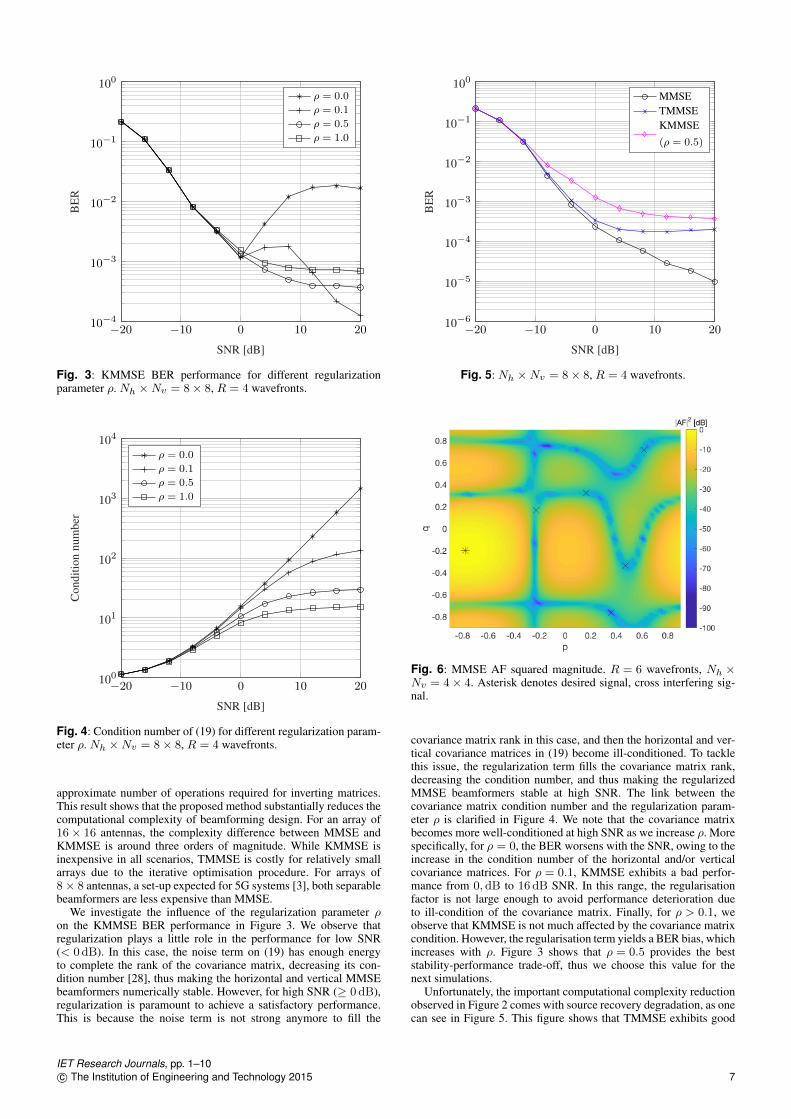
Fig. 5: Nh ×Nv = 8× 8, R = 4 wavefronts.

Fig. 6: MMSE AF squared magnitude. R = 6 wavefronts, Nh ×Nv = 4× 4. Asterisk denotes desired signal, cross interfering sig-nal.

covariance matrix rank in this case, and then the horizontal and ver-tical covariance matrices in (19) become ill-conditioned. To tacklethis issue, the regularization term fills the covariance matrix rank,decreasing the condition number, and thus making the regularizedMMSE beamformers stable at high SNR. The link between thecovariance matrix condition number and the regularization param-eter ρ is clarified in Figure 4. We note that the covariance matrixbecomes more well-conditioned at high SNR as we increase ρ. Morespecifically, for ρ = 0, the BER worsens with the SNR, owing to theincrease in the condition number of the horizontal and/or verticalcovariance matrices. For ρ = 0.1, KMMSE exhibits a bad perfor-mance from 0, dB to 16 dB SNR. In this range, the regularisationfactor is not large enough to avoid performance deterioration dueto ill-condition of the covariance matrix. Finally, for ρ > 0.1, weobserve that KMMSE is not much affected by the covariance matrixcondition. However, the regularisation term yields a BER bias, whichincreases with ρ. Figure 3 shows that ρ = 0.5 provides the beststability-performance trade-off, thus we choose this value for thenext simulations.

Unfortunately, the important computational complexity reductionobserved in Figure 2 comes with source recovery degradation, as onecan see in Figure 5. This figure shows that TMMSE exhibits good


Fig. 7: TMMSE AF squared magnitude. R = 6 wavefronts, Nh ×Nv = 4× 4. Asterisk denotes desired signal, cross interfering sig-nal.

Fig. 8: KMMSE AF squared magnitude. R = 6 wavefronts, Nh ×Nv = 4× 4, ρ = 0.5. Asterisk denotes desired signal, cross inter-fering signal.

performance from−20 dB to 0 dB, while KMMSE with regulariza-tion parameter ρ = 0.5 performs similarly to the benchmark onlyfrom −20 dB to −8 dB. At high SNR, the BER performance of theseparable beamformers is heavily penalized compared to the bench-mark. When one of the direction cosines (pr or qr) of the interferingwavefronts is adjacent to those of the desired signal, the separablebeamformers fail to recover it, yielding a significant number of biterrors. Since the direction cosines of all wavefronts are randomlyselected according to a uniform distribution, it is rather commonthat the interfering wavefronts are close to the desired signal ineither p- or q-domain. As a consequence, beamforming fails dueto ill-conditioned covariance matrices, as discussed in the previousparagraph. At high SNR, the poor BER performance is especiallyaccentuated because the noise component does not have enoughpower to fill the covariance matrix rank. However, whenever thewavefronts are sufficiently separated in space, the separable beam-formers exhibit good source recovery performance. The presentedresults suggest that the proposed methods are appealing alternativesto the standard MMSE beamformer. In Figure 2, the computationalcomplexity of KMMSE, for example, is two orders of magnitudesmaller than that of MMSE for Nh ×Nv = 8× 8. On the otherhand, Figure 5 indicates that KMMSE is 5 dB apart from MMSEfor the uncoded BER of 10−3.

Fig. 9: Horizontal KMMSE AF squared magnitude. R = 6 wave-fronts, Nh = 4, ρ = 0.5. Asterisk denotes desired signal, crossinterfering signal.

Fig. 10: Vertical KMMSE AF squared magnitude. R = 6 wave-fronts, Nv = 4, ρ = 0.5. Asterisk denotes desired signal, crossinterfering signal.

To better understand why the separable beamformers are moresensitive to closely-spaced wavefronts, let us investigate their nor-malised array factor. We consider a scenario in which the proposedbeamformers fail due to lack of degrees of freedom. For visualisa-tion easiness, we consider a scenario where a 4× 4 array is appliedto filter R = 6 wavefronts in the following. In this case, each sub-array beamformer has only 4 degrees of freedom and will fail to filtertheR = 6 signals. By contrast, the classical MMSE beamformer has16 degrees of freedom and is able to null the interfering wavefrontsand recover the desired signal. Figures 6, 7, and 8 show the magni-tude of the MMSE, TMMSE, and KMMSE normalised array factorsas functions of the direction cosines, respectively. One can see thatthe MMSE filter accurately places nulls at the interfering wavefrontsdirections, while a strong beam is pointed towards the desired sig-nal. This is possible because the 16-dimensional filter has sufficientdegrees of freedom to separate the wavefronts. In contrast to thebenchmark method, KMMSE does not accurately distribute nulls,hindering interference attenuation. In Figures 9 and 10, one can seethat the KMMSE sub-beamformers do not have enough degrees offreedom to attenuate the interfering wavefronts. As a consequence,the undesired signal at (p, q) = (0.5,−0.3) is not properly attenu-ated, as seen in Figure 8. We observe that only 3 nulls are placed toattenuate 5 interfering wavefronts in Figure 9. The same is observed


in Figure 10. To solve this issue, one would need to increase the num-ber of antennas to, at least, Nh ×Nv = 6× 6. Figure 7 reveals thatTMMSE is more accurate than KMMSE at null placement. This isbecause the null locations are optimised as the alternating algorithmiterates. This accuracy is important especially at high SNR, as onecan see in Figure 5. We conclude that the separable beamformersare more sensitive to the number of impinging signals and closelyspaced wavefronts than the classical MMSE beamformer due to thereduced degrees of freedom of the sub-beamformers.

5 Conclusion

We presented two beamforming methods that exploit array separa-bility to reduce the computational complexity of the classical MMSEbeamformer. The TMMSE filter is based on tensor algebra and min-imises the MMSE by means of alternating minimisation, while theKMMSE filter relies on regularized sub-array MMSE beamforming.Our simulation results show that TMMSE provides moderate com-putational complexity reduction with small source recovery degra-dation. By contrast, KMMSE is computationally inexpensive butexhibits poorer BER performance at high SNR. Therefore, TMMSEshould be employed when source recovery performance is moreimportant than computation efficiency, and KMMSE on the contrary.This work paves the way to future contributions, including the exten-sion to massive MIMO architectures, e.g., hybrid analogue/digitaltransceivers. Furthermore, it would be of interest to validate the pro-posed methods with array responses simulated in an electromagneticfield simulator software.

6 Appendix

It is well-known that the minimisers of (14) and (15) are given bythe classical MMSE filters wh = R−1hhphs and wv = R−1vv pvs,respectively. In this appendix, we obtain the covariance matricesand cross-covariance vectors necessary to calculate these filters. Inour demonstrations, we consider only the horizontal sub-array. Thestatistics for the vertical sub-array are analogously derived.

First, let us represent (9) in terms of the matrix unfoldings of A.Unfolding this tensor along its first mode gives [22]

X[k] = [A](1)(s[k]⊗ INv) + B[k].

Now the horizontal sub-array input (12) can be expressed as

uh[k](a)=[[A](1)(s[k]⊗ INv

) + B[k]]

(1⊗w∗v)

(b)= [A](1)(s[k]⊗w∗v) + B[k]w∗v , (26)

where (a) follows by considering w∗v = 1⊗w∗v , and (b) is theapplication of the mixed product property [24]:

(A⊗B)(C ⊗D) = (AC)⊗ (BD)

for any matrices A, B, C, D with matching dimensions. Thecovariance matrix of (26) is then given by

Rhh = [A](1)(Rss ⊗w∗vwTv )[A]H(1) + Rcc,

where Rcc = E[c[k]cH[k]

], and c[k] = B[k]w∗v ∈ CNh . Note we

have used the fact that E [A⊗B] = E [A]⊗ E [B] for matricesA and B with mutually independent elements, and that the inputsof B[k] and s[k] are uncorrelated. To calculate Rcc, consider the

element-wise representation of c[k]:

[c[k]]nh =

Nv∑nv=1

[B[k]]nh,nv [wv]∗nv, nh ∈ {1, . . . , Nh}.

The elements of Rcc are given by:

[Rcc]nh,n′h= E

[[c[k]]nh [c[k]H]n′h

]= E

Nv∑nv=1

Nv∑n′v=1

[B[k]]nh,nv[B[k]]∗n′h,n′v

[wv]nv[wv]∗n′v

for nh, n

′h ∈ {1, . . . , Nh}. As the AWGN vector has mutually

independent elements, it follows that

E[[B[k]]nh,nv

[B[k]]∗n′h,n′v

]= 0

for all nv 6= n′v and nh 6= n′h. Therefore, the off-diagonal elementsof Rcc are zero and those at the main diagonal are given by

[Rcc]nh,nh =

Nv∑nv=1

E[[B[k]]nh,nv

[B[k]]∗nh,nv

][wv]nv

[wv]∗nv

+ σ2b

Nv∑nv=1

[wv]nv[wv]∗nv

= σ2b‖wv‖22

and, consequently, we get Rcc = σ2b‖wv‖22INh

, concluding thederivation of Rhh. From the definition of phs and uh[k], it followsthat:

phs = E[(

[A](1)(s[k]⊗w∗v) + B[k]w∗v)

(s∗d[k]⊗ 1)]

= [A](1)(s[k]s∗d[k]⊗w∗v) = [A](1)(Rssed ⊗w∗v),

finalising our proof. �

Acknowledgment

This work is supported by the National Council for Scientific andTechnological Development – CNPq, CAPES/PROBRAL Proc. no.88887.144009/2017-00, and FUNCAP.

7 References1 E. G. Larsson, O. Edfors, F. Tufvesson, and T. L. Marzetta, “Massive MIMO for

next generation wireless systems,” IEEE Communications Magazine, vol. 52, no. 2,pp. 186–195, Feb. 2014.

2 S. Schwarz and M. Rupp, “Society in motion: challenges for LTE and beyondmobile communications,” IEEE Communications Magazine, vol. 54, no. 5, pp. 76–83, May 2016.

3 H. Ji, Y. Kim, J. Lee, E. Onggosanusi, Y. Nam, J. Zhang, B. Lee, and B. Shim,“Overview of full-dimension MIMO in LTE-advanced pro,” IEEE Communica-tions Magazine, vol. 55, no. 2, pp. 176–184, 2017.

4 L. N. Ribeiro, S. Schwarz, M. Rupp, and A. L. de Almeida, “Energy efficiency ofmmWave massive MIMO precoding with low-resolution DACs,” IEEE Journal ofSelected Topics in Signal Processing, vol. 12, no. 2, pp. 298–312, 2018.

5 S. Treitel and J. L. Shanks, “The design of multistage separable planar filters,”IEEE Transactions on Geoscience Electronics, vol. 9, no. 1, pp. 10–27, 1971.

6 M. Boussé, O. Debals, and L. De Lathauwer, “A tensor-based method for large-scale blind source separation using segmentation,” IEEE Transactions on SignalProcessing, vol. 65, no. 2, pp. 346–358, 2017.

7 M. Rupp and S. Schwarz, “A tensor LMS algorithm,” in Proc. 2015 IEEE Inter-national Conference on Acoustics, Speech and Signal Processing (ICASSP), 2015,pp. 3347–3351.

8 ——, “Gradient-based approaches to learn tensor products,” in Proc. 2015 23rdEuropean Signal Processing Conference (EUSIPCO), 2015, pp. 2486–2490.

9 F. C. Pinheiro and C. G. Lopes, “Nonlinear adaptive algorithms on rank-one tensormodels,” arXiv preprint arXiv:1610.07520, 2016.


10 L. N. Ribeiro, A. L. de Almeida, and J. C. M. Mota, “Identification of sepa-rable systems using trilinear filtering,” in Proc. of the 2015 IEEE 6th Interna-tional Workshop on Computational Advances in Multi-Sensor Adaptive Processing(CAMSAP), pp. 189–192.

11 C. Paleologu, J. Benesty, and S. Ciochina, “Linear system identification based ona Kronecker product decomposition,” IEEE/ACM Transactions on Audio, Speech,and Language Processing, 2018.

12 C. Elisei-Iliescu, C. Stanciu, C. Paleologu, J. Benesty, C. Anghel, and S. Ciochina,“Efficient recursive least-squares algorithms for the identification of bilinearforms,” Digital Signal Processing, vol. 83, pp. 280–296, 2018.

13 H. L. Van Trees, Optimum array processing: Part IV of detection, estimation andmodulation theory. Wiley Online Library, 2002, vol. 1.

14 Z. Wang, W. Liu, C. Qian, S. Chen, and L. Hanzo, “Two-dimensional precoding for3-D massive MIMO,” IEEE Transactions on Vehicular Technology, vol. 66, no. 6,pp. 5485–5490, Jun. 2017.

15 G. Zhu, K. Huang, V. K. Lau, B. Xia, X. Li, and S. Zhang, “Hybrid beamformingvia the Kronecker decomposition for the millimeter-wave massive MIMO sys-tems,” IEEE Journal on Selected Areas in Communications, vol. 35, no. 9, pp.2097–2114, 2017.

16 R. K. Miranda, J. P. C. da Costa, F. Roemer, A. L. de Almeida, and G. Del Galdo,“Generalized sidelobe cancellers for multidimensional separable arrays,” in Com-putational Advances in Multi-Sensor Adaptive Processing (CAMSAP), 2015 IEEE6th International Workshop on. IEEE, 2015, pp. 193–196.

17 L. Liu, J. Xie, L. Wang, Z. Zhang, and Y. Zhu, “Robust tensor beamforming forpolarization sensitive arrays,” Multidimensional Systems and Signal Processing,pp. 1–22, 2018.

18 L. N. Ribeiro, S. Schwarz, M. Rupp, A. L. F. de Almeida, and J. C. M. Mota, “Alow-complexity equalizer for massive MIMO systems based on array separabil-ity,” in Proc. 2017 25th European Signal Processing Conference (EUSIPCO), pp.2522–2526.

19 S. Haykin, “Adaptive filtering theory,” Englewood Cliffs, NJ: Prentice-Hall, 1996.20 K. B. Petersen and M. S. Pedersen, “The matrix cookbook,” 2012.21 L. N. Ribeiro, A. L. F. De Almeida, and J. C. M. Mota, “Tensor beamforming

for multilinear translation invariant arrays,” in Proc. 2016 IEEE InternationalConference on Acoustics, Speech and Signal Processing (ICASSP), 2016, pp.2966–2970.

22 T. Kolda and B. Bader, “Tensor decompositions and applications,” SIAM Review,vol. 51, no. 3, pp. 455–500, Aug. 2009.

23 P. Comon, X. Luciani, and A. L. De Almeida, “Tensor decompositions, alternat-ing least squares and other tales,” Journal of Chemometrics: A Journal of theChemometrics Society, vol. 23, no. 7-8, pp. 393–405, 2009.

24 S. Liu and G. Trenkler, “Hadamard, Khatri-Rao, Kronecker and other matrix prod-ucts,” International Journal of Information and Systems Sciences, vol. 4, no. 1, pp.160–177, 2008.

25 D. P. Palomar and Y. C. Eldar, Convex optimization in signal processing andcommunications. Cambridge university press, 2010.

26 A. Yener, R. D. Yates, and S. Ulukus, “Interference management for CDMAsystems through power control, multiuser detection, and beamforming,” IEEETransactions on Communications, vol. 49, no. 7, pp. 1227–1239, 2001.

27 T. Minka, “The Lightspeed MATLAB toolbox, version 2.8,” 2017. [Online].Available: https://github.com/tminka/lightspeed

28 G. H. Golub and C. F. Van Loan, Matrix computations. JHU Press, 2012, vol. 3.


Documents

Low-Complexity Separable Beamformers for Massive Antenna