Low-Rank Matrices

(aka Spectral Methods)

Sujay Sanghavi

ECE University of Texas, Austin

Outline

1.  Background - Low-rank Matrices, Eigenvalues, eigenvectors, etc.

2.  Principal Components Analysis

3.  Spectral Clustering

4.  Predictions / collaborative filtering

5.  Structured low-rank matrices: NNMF, Sparse PCA etc.

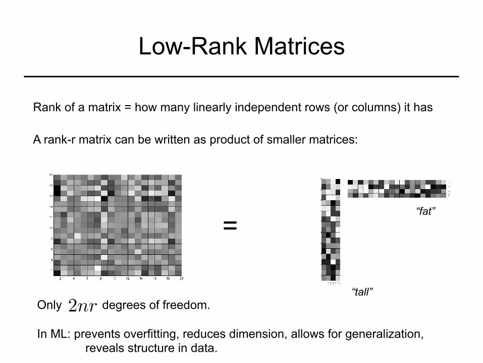
Low-Rank Matrices

Rank of a matrix = how many linearly independent rows (or columns) it has

A rank-r matrix can be written as product of smaller matrices:

Only degrees of freedom. In ML: prevents overfitting, reduces dimension, allows for generalization,

reveals structure in data.

=

2nr“tall”

“fat”

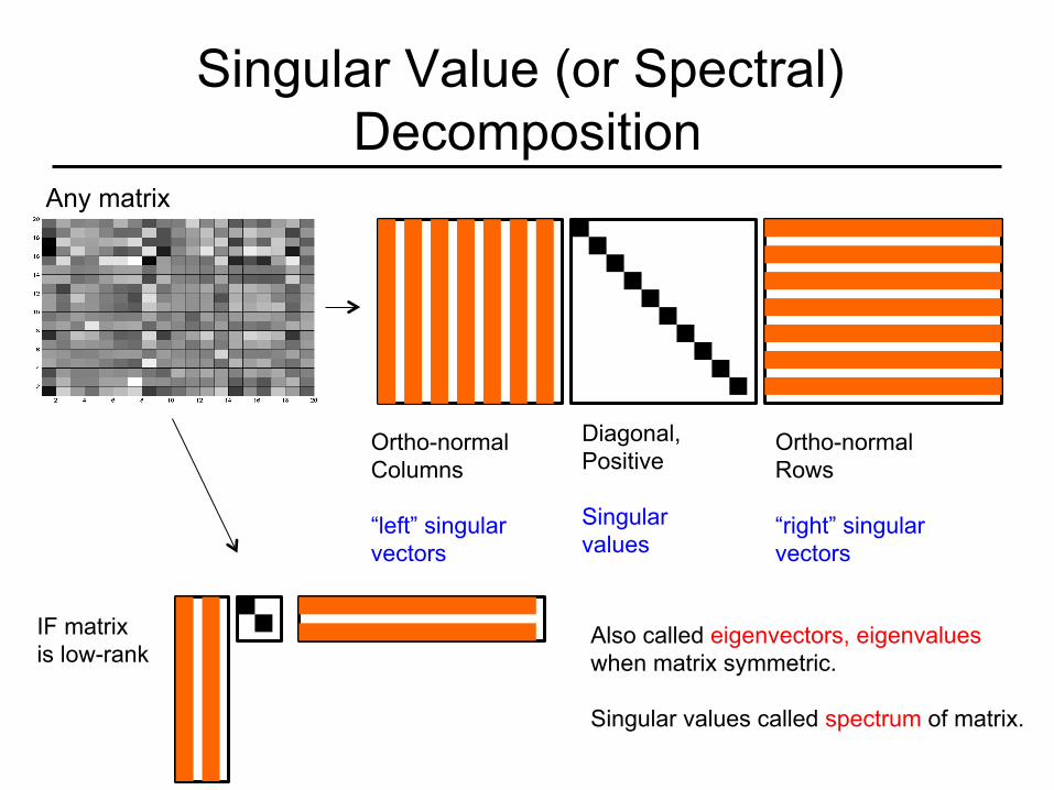
Singular Value (or Spectral) Decomposition

Ortho-normal Columns “left” singular vectors

Diagonal, Positive Singular values

Ortho-normal Rows “right” singular vectors

Any matrix

IF matrix is low-rank

Also called eigenvectors, eigenvalues when matrix symmetric. Singular values called spectrum of matrix.

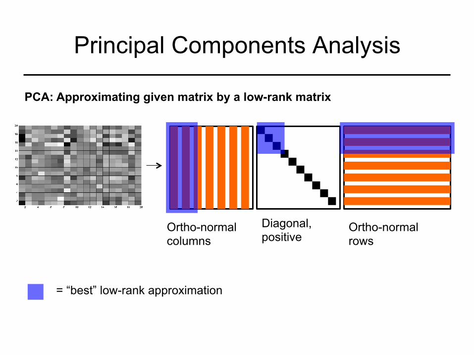
Principal Components Analysis

Ortho-normal columns

Diagonal, positive

Ortho-normal rows

= “best” low-rank approximation

PCA: Approximating given matrix by a low-rank matrix

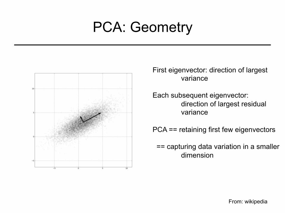
PCA: Geometry

First eigenvector: direction of largest variance

Each subsequent eigenvector:

direction of largest residual variance

PCA == retaining first few eigenvectors == capturing data variation in a smaller

dimension

From: wikipedia

Uses of PCA: Visualization

Each country a 3-d vector (area, avg. income, population) Then take top-2 PCA

From: wikipedia

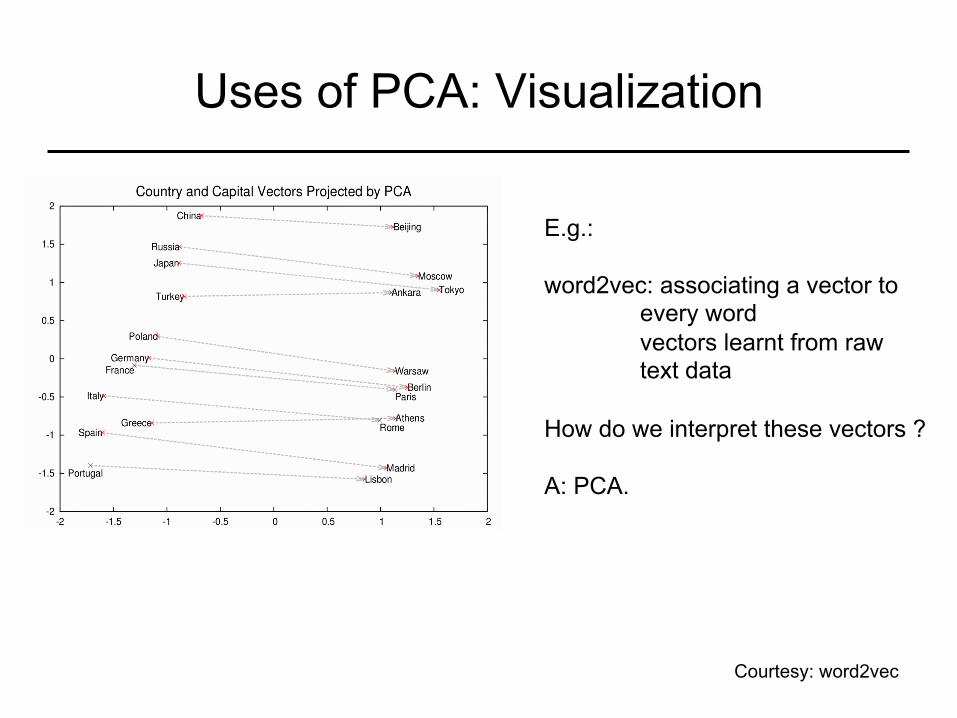
Uses of PCA: Visualization

E.g.: word2vec: associating a vector to

every word vectors learnt from raw text data

How do we interpret these vectors ? A: PCA.

Courtesy: word2vec

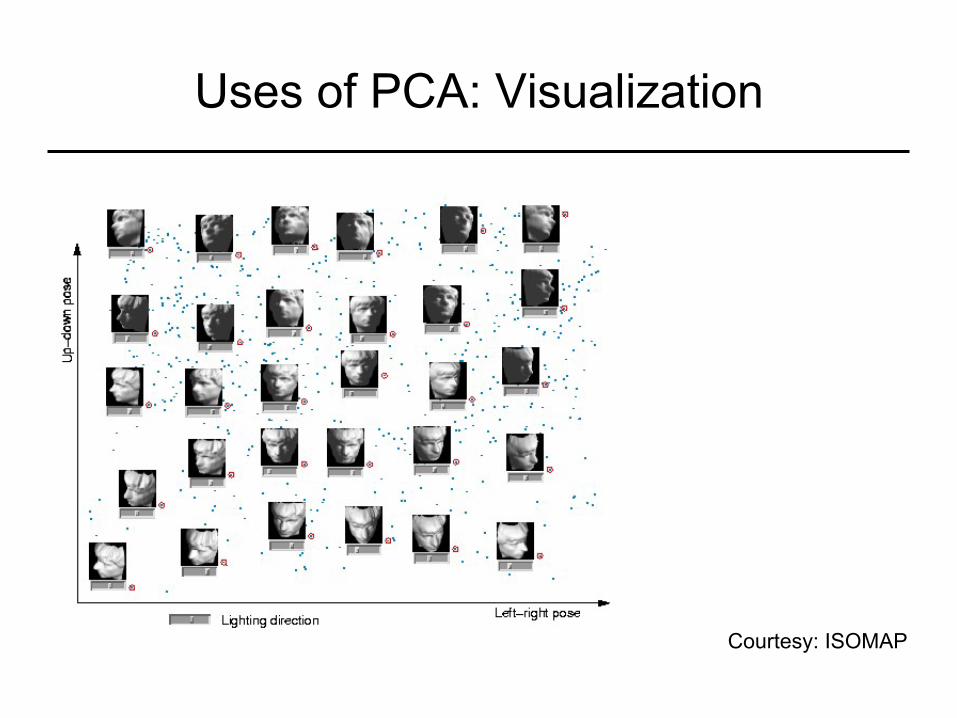
Uses of PCA: Visualization

Courtesy: ISOMAP

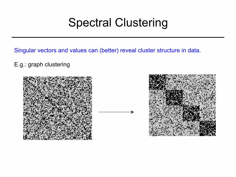
Spectral Clustering

Singular vectors and values can (better) reveal cluster structure in data. E.g.: graph clustering

Spectral Clustering

1.  Organize data into matrix: each column is one data point

2.  Find top r “left” singular vectors. This is the top-r subspace.

3.  Represent each data point as a vector in by projecting onto this subspace.

4.  Do some “naïve” clustering of these vectors in

Rr

Rr

subspace projections

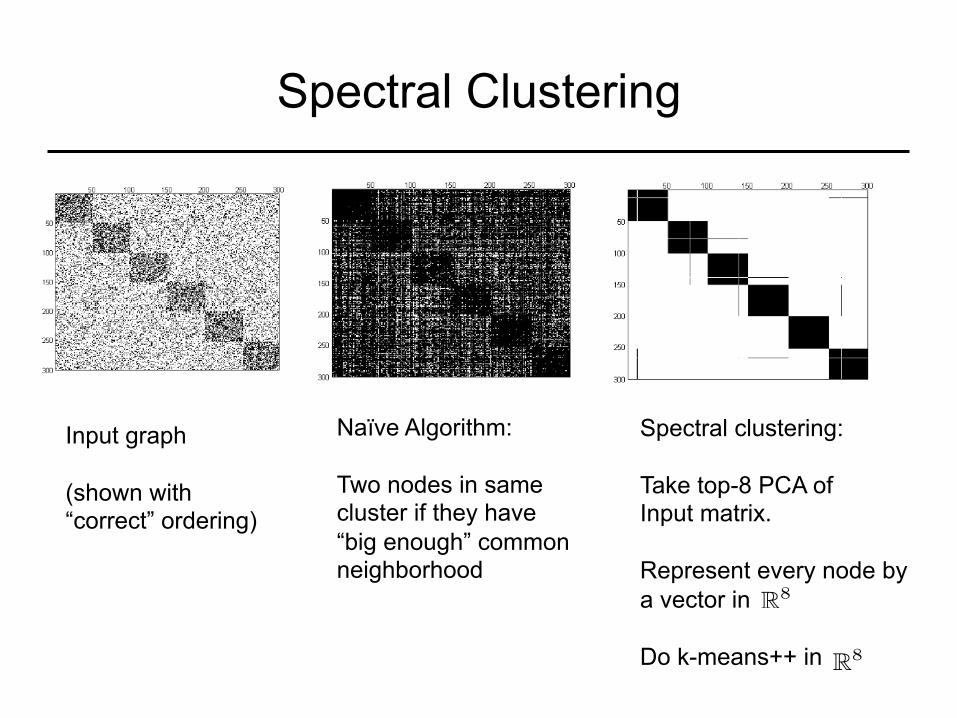
Spectral Clustering

Naïve Algorithm: Two nodes in same cluster if they have “big enough” common neighborhood

Spectral clustering: Take top-8 PCA of Input matrix. Represent every node by a vector in Do k-means++ in

R8

R8

Input graph (shown with “correct” ordering)

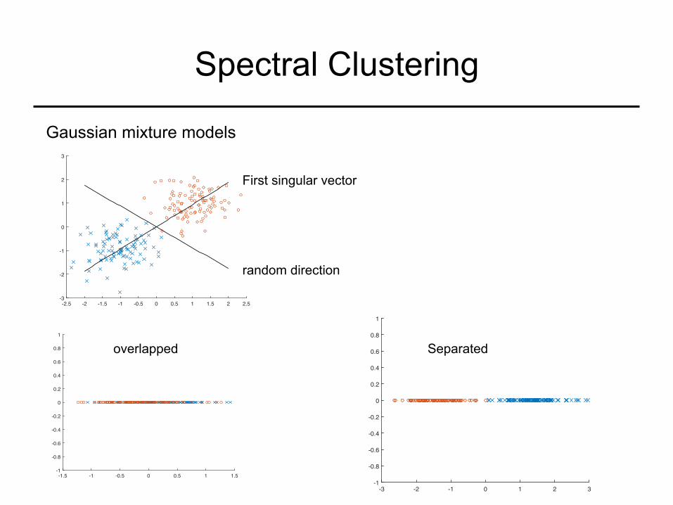
Spectral Clustering

Gaussian mixture models

-2.5 -2 -1.5 -1 -0.5 0 0.5 1 1.5 2 2.5-3

-2

-1

0

1

2

3

Given: Unlabeled points from several different Gaussian distributions

Task: Find means of these Gaussians. Spectral clustering: Retains “direction of separation”, removes other directions (and noise therein)

Spectral Clustering

Gaussian mixture models

-2.5 -2 -1.5 -1 -0.5 0 0.5 1 1.5 2 2.5-3

-2

-1

0

1

2

3

-1.5 -1 -0.5 0 0.5 1 1.5-1

-0.8

-0.6

-0.4

-0.2

0

0.2

0.4

0.6

0.8

1

-3 -2 -1 0 1 2 3-1

-0.8

-0.6

-0.4

-0.2

0

0.2

0.4

0.6

0.8

1

random direction

First singular vector

overlapped Separated

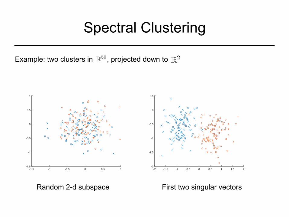
Spectral Clustering

-2 -1.5 -1 -0.5 0 0.5 1 1.5 2-2

-1.5

-1

-0.5

0

0.5

-1.5 -1 -0.5 0 0.5 1-1.5

-1

-0.5

0

0.5

1

Example: two clusters in , projected down to R50 R2

Random 2-d subspace First two singular vectors

Spectral Clustering

More general settings:

1.  Make pairwise similarity matrix

2.  Find top r singular vectors of similarity matrix

3.  Represent each point as a vector in

4.  Run k-means or other simple method

Rr

sij = e�dij

“kernel trick”

Matrix Completion

1

3

4

10

7 5 2 1

7 5 2 1

70 50 20 10

21 15 6 3

28 20 8 4

Task: given few elements of a matrix, find the remaining elements NOT possible in general. MAY be possible for low-rank matrix – because few degrees of freedom. Applications: in a couple of slides …

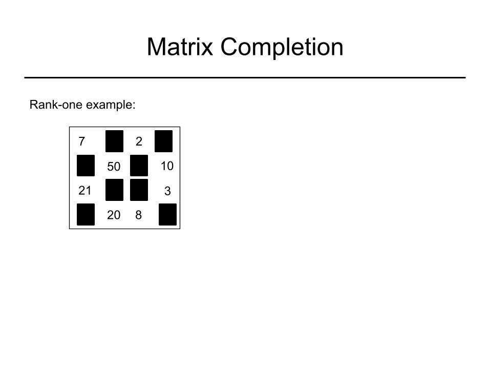
Matrix Completion

7 5 2 1

70 50 20 10

21 15 6 3

28 20 8 4

Rank-one example:

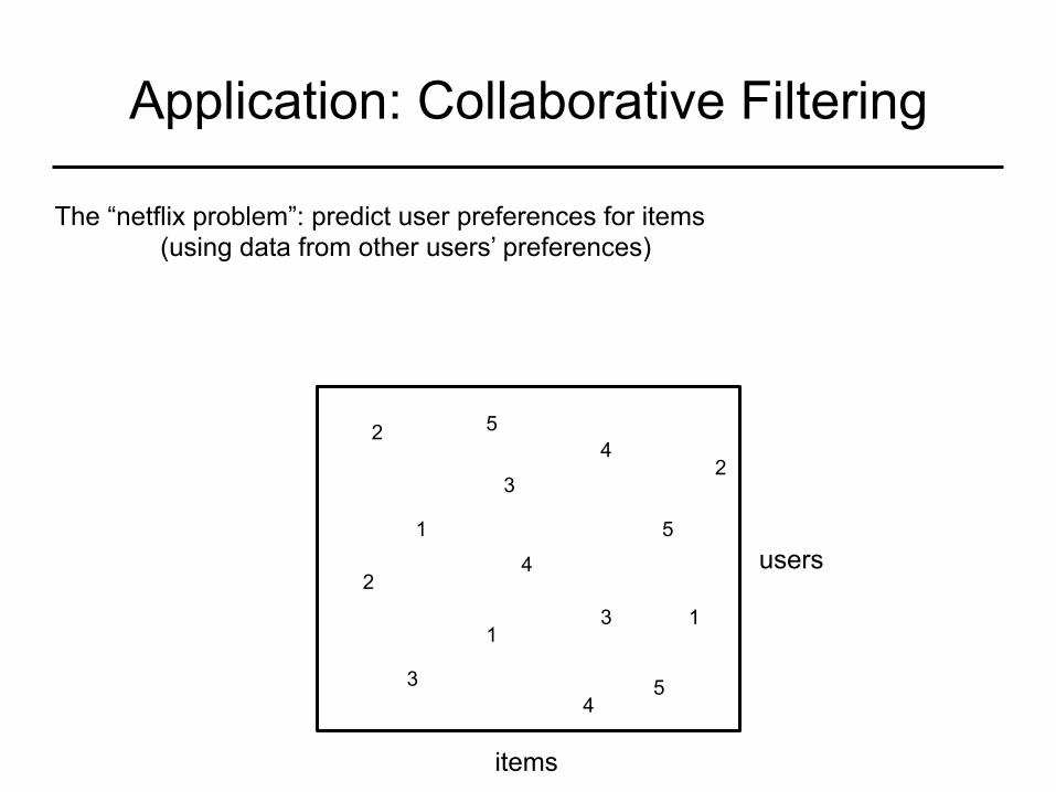
Application: Collaborative Filtering

The “netflix problem”: predict user preferences for items (using data from other users’ preferences)

users

items

5

2

3

1

4

5

2

3

1

4 5

2

3

1

4

Application: Collaborative Filtering

Low rank == a “small number of hidden factors” govern our likes and dislikes

users

items

5

2

3

1

4

5

2

3

1

4 5

2

3

1

4

mij ⇡ f(hui, vji)

Matrix Completion

Most popular method: Alternating Least Squares:

minU,V

X

(i,j)2⌦

(mij � hui, vji)2

U

V 0

Iteratively and alternately: hold one of U (or V) fixed, solve least-squares for the other Fast, parellel / distributed etc. If link function f non-linear, do Alternating Minimization. Very recently: theoretical guarantees on when this works.

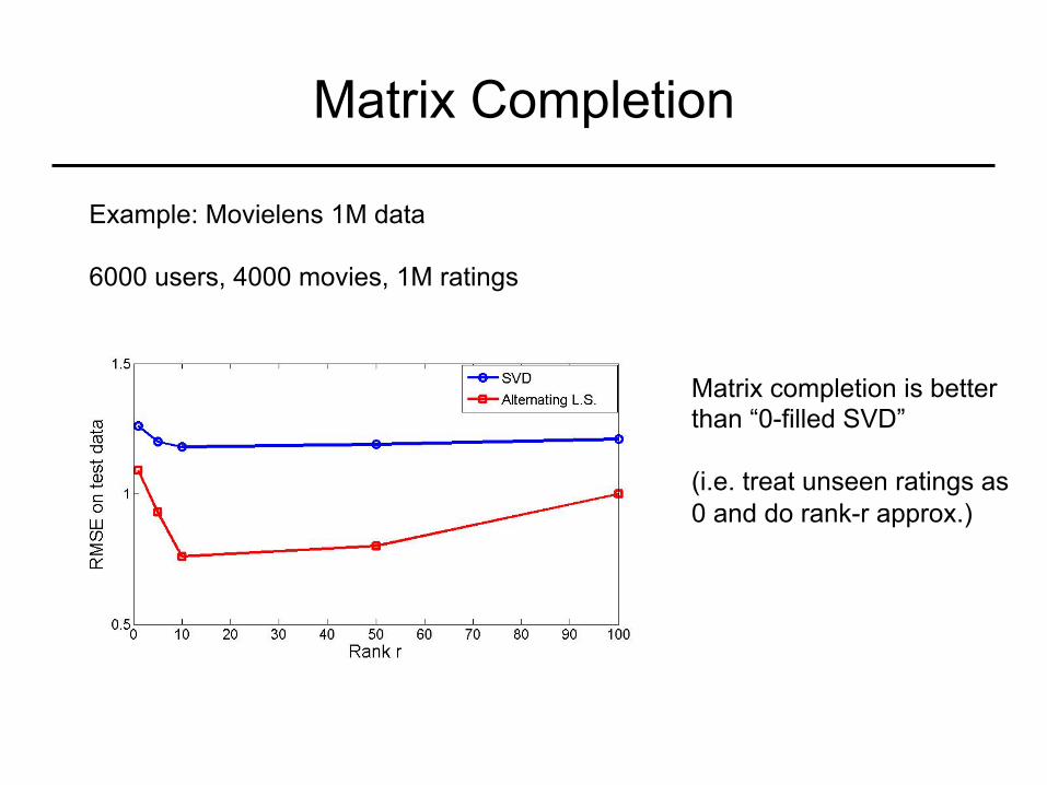
Matrix Completion

Example: Movielens 1M data 6000 users, 4000 movies, 1M ratings

Matrix completion is better than “0-filled SVD” (i.e. treat unseen ratings as 0 and do rank-r approx.)

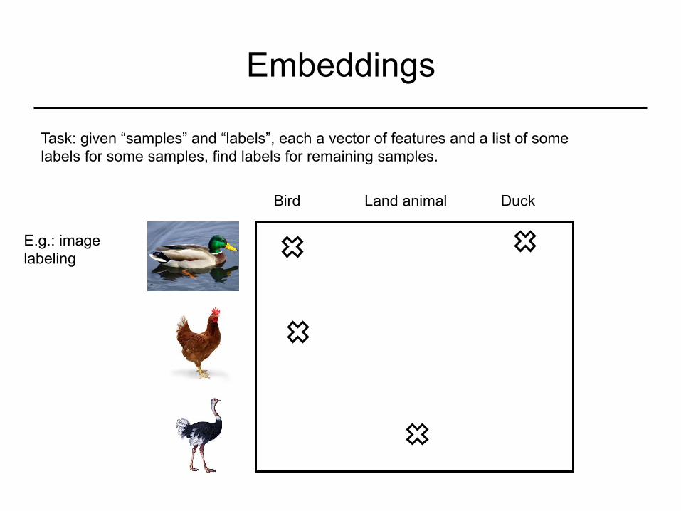
Embeddings

E.g.: image labeling

Bird Land animal Duck

Task: given “samples” and “labels”, each a vector of features and a list of some labels for some samples, find labels for remaining samples.

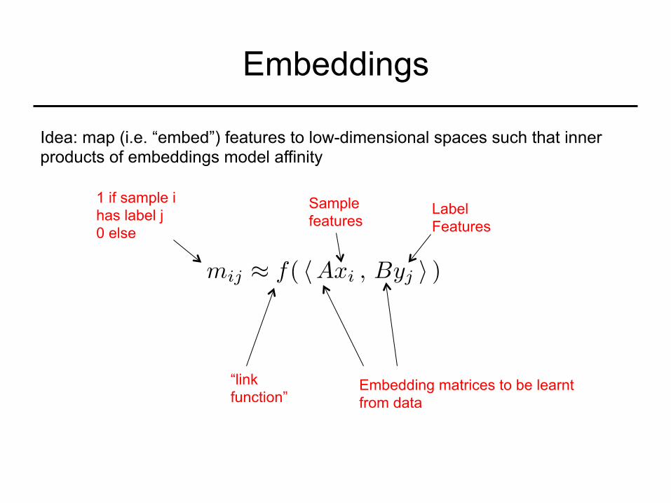
Embeddings

Idea: map (i.e. “embed”) features to low-dimensional spaces such that inner products of embeddings model affinity

mij ⇡ f( hAxi , Byj i )

1 if sample i has label j 0 else

“link function”

Embedding matrices to be learnt from data

Sample features

Label Features

Embeddings

0 0.05 0.1 0.15 0.2 0.25 0.3 0.35 0.414

16

18

20

22

24

26

28

30

32

34

D/L (bibtex)

%

<Train> P@3(iter#30000)max(WSABIE): 32.94%

max(MELR): 20.28%

WSABIEMELR

0 0.05 0.1 0.15 0.2 0.25 0.3 0.35 0.415

20

25

30

D/L (bibtex)

%

<Validation> P@3(iter#30000)max(WSABIE): 28.94%

max(MELR): 18.98%

WSABIEMELR

0 0.05 0.1 0.15 0.2 0.25 0.3 0.35 0.415

20

25

30

D/L (bibtex)

%

<Test> P@3(iter#30000)max(WSABIE): 29.03%

max(MELR): 19.07%

WSABIEMELR

Example: predicting missing authors of documents “sample”: a paper. Features: words in the title, abstract. “label”: author name. Features: university, department, etc.

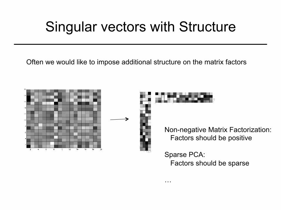
Singular vectors with Structure

Often we would like to impose additional structure on the matrix factors

Non-negative Matrix Factorization: Factors should be positive Sparse PCA: Factors should be sparse …

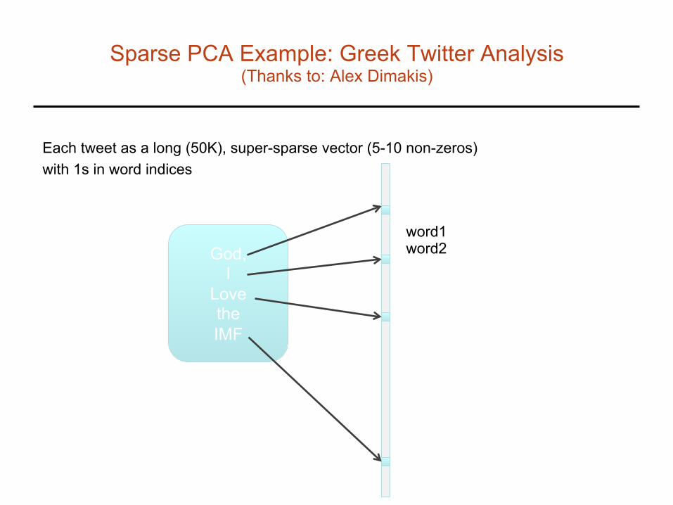
Sparse PCA Example: Greek Twitter Analysis (Thanks to: Alex Dimakis)

Each tweet as a long (50K), super-sparse vector (5-10 non-zeros) with 1s in word indices

God, I

Love the IMF

word1 word2

word n

Data Sample Matrix

We collect all tweet vectors in a sample matrix of size

m tweets

S = n words

n⇥m

. . .

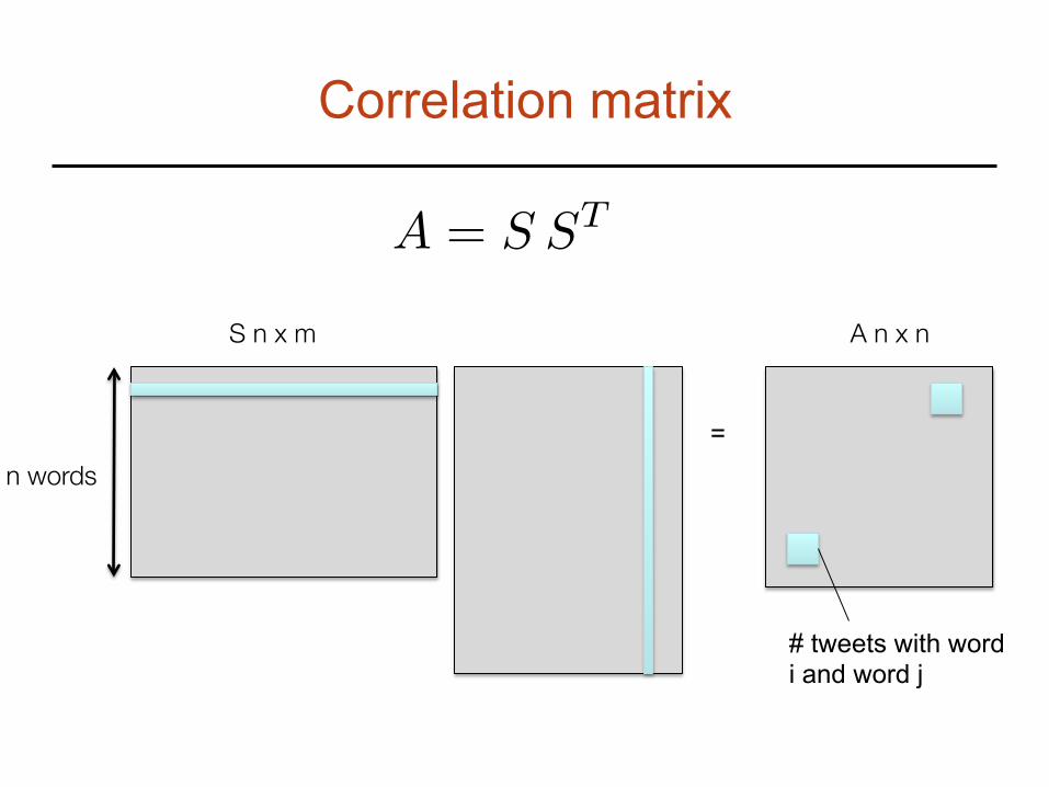
Correlation matrix

A = S ST

n words =

A n x n S n x m

# tweets with word i and word j

vanilla PCA

Largest Eigenvector. Maximizes `explained variance’ of the data set Very useful for dimensionality reduction Easy to compute

PCA finds An `EigenTweet’

Finds a vector that closely matches most tweets i.e, a vector that maximizes the sum of projections with each tweet

⇥

max kxTSk2

. . .

The problem with PCA

•  Top Eigenvector will be dense!

32

Eurovision Protests Greece Morning

Deals Engage Offers

Uprising Protest

Elections teachers Summer support Schools

.

.

. Crisis

Earthquake IMF

Dense = A tweet with thousands of words

(makes no sense)

0.1 0.02

.

.

.

0.001

The problem with PCA

•  Top Eigenvector will be dense!

•  We want super sparse Sparse = Interpretable

33

Strong Earthquake

Greece Morning

Eurovision Protests Greece Morning

Deals Engage Offers

Uprising Protest

Elections teachers Summer support Schools

.

.

. Crisis

Earthquake IMF

Dense = A tweet with thousands of words

(makes no sense)

0.1 0.02

.

.

.

0.001

0.75 0.49 0.23 0.31

Experiments (5 days in May 2011)

skype, microsoft, acquisition, billion, acquired, acquires, buy, dollars, acquire, google

eurovision greece lucas finals final stereo semifinal contest greek watching

love received greek know damon amazing hate twitter great sweet

downtown athens murder years brutal stabbed incident camera year crime

k=10, top 4 sparse PCs for the data set (65,000 tweets)

Summary

Low-rank matrices have a lot of algebraic structure The are widely used in data analysis and machine learning

- visualization - preprocessing data and dimensionality reduction - to prevent over-fitting in prediction - to reveal insights from data

Research Directions:

- algorithm design for matrix factorizations w/ extra structure - theoretical analyses (esp. statistical guarantees) - big-data settings (e.g. one-pass or two-pass algorithms) - applications

Thanks !