Online Learning in the Embedded Manifold of Low-rank Matrices

Journal of Machine Learning Research 13 (2012) 429-458 Submitted 6/11; Revised 11/11; Published 2/12

Online Learning in the Embedded Manifold of Low-rank Matrices

Uri Shalit ∗ URI.SHALIT@MAIL .HUJI.AC.ILComputer Science Department and ICNC/ELSCThe Hebrew University of Jerusalem91904 Jerusalem, Israel

Daphna Weinshall [email protected] Science DepartmentThe Hebrew University of Jerusalem91904 Jerusalem, Israel

Gal Chechik† [email protected]

The Gonda Brain Research CenterBar Ilan University52900 Ramat-Gan, Israel

Editor: Léon Bottou

AbstractWhen learning models that are represented in matrix forms, enforcing a low-rank constraint candramatically improve the memory and run time complexity, while providing a natural regularizationof the model. However, naive approaches to minimizing functions over the set of low-rank matricesare either prohibitively time consuming (repeated singular value decomposition of the matrix) ornumerically unstable (optimizing a factored representation of the low-rank matrix). We build onrecent advances in optimization over manifolds, and describe an iterative online learning procedure,consisting of a gradient step, followed by asecond-order retractionback to the manifold. Whilethe ideal retraction is costly to compute, and so is the projection operator that approximates it, wedescribe another retraction that can be computed efficiently. It has run time and memory complexityof O((n+m)k) for a rank-k matrix of dimensionm× n, when using an online procedure withrank-one gradients. We use this algorithm, LORETA, to learn a matrix-form similarity measureover pairs of documents represented as high dimensional vectors. LORETA improves the meanaverage precision over a passive-aggressive approach in a factorized model, and also improves overa full model trained on pre-selected features using the samememory requirements. We furtheradapt LORETA to learn positive semi-definite low-rank matrices, providing an online algorithmfor low-rank metric learning. LORETA also shows consistent improvement over standard weaklysupervised methods in a large (1600 classes and 1 million images, usingImageNet) multi-labelimage classification task.Keywords: low rank, Riemannian manifolds, metric learning, retractions, multitask learning,online learning

1. Introduction

Many learning problems involve models represented in matrix form. These include metric learning,collaborative filtering, and multi-task learning where all tasks operate overthe same set of features.

∗. Also at The Gonda Brain Research Center, Bar Ilan University, 52900 Ramat-Gan, Israel.†. Also at Google Research, 1600 Amphitheatre Parkway, Mountain ViewCA, 94043.

c©2012 Uri Shalit, Daphna Weinshall and Gal Chechik.

SHALIT , WEINSHALL AND CHECHIK

In many of these tasks, a natural way to regularize the model is to limit the rank of the correspondingmatrix. In metric learning, a low-rank constraint allows to learn a low dimensional representationof the data in a discriminative way. In multi-task problems, low-rank constraintsprovide a way totie together different tasks. In all cases, low-rank matrices can be represented in a factorized formthat dramatically reduces the memory and run-time complexity of learning and inference with thatmodel. Low-rank matrix models could therefore scale to handle substantially many more featuresand classes than models with full rank dense matrices.

Unfortunately, the rank constraint is non-convex, and in the general case, minimizing a convexfunction subject to a rank constraint is NP-hard (Natarajan, 1995).1 As a result of these issues, twomain approaches have been commonly used to address the problem of learning under a low-rankconstraint. Sometimes, a matrixW ∈ R

n×m of rankk is represented as a product of two low dimen-sion matricesW = ABT ,A∈ R

n×k,B∈ Rm×k and simple gradient descent techniques are applied to

each of the product terms separately (Bai et al., 2009). Second, projected gradient algorithms canbe applied by repeatedly taking a gradient step and projecting back to the manifold of low-rankmatrices. Unfortunately, computing the projection to that manifold becomes prohibitively costly forlarge matrices and cannot be computed after every gradient step.

Work in the field has focused mostly on two realms. First, learning low-rank positive semi-definite (PSD) models (as opposed to general low-rank models), as in the works of Kulis et al.(2009) and Meyer et al. (2011). Second, approximating a noisy matrix ofobservations by a low-rank matrix, as in the work of Negahban and Wainwright (2010). This taskis commonly addressedin the field of recommender systems. Importantly, the current paper does not address the problemof low-rank approximation to a given data matrix, but rather addresses the problem of learning alow-rank parametric modelin the context of ranking and classification.

In this paper we propose new algorithms for online learning on the manifold oflow-rank matri-ces. It is based on an operation calledretraction, which is an operator that maps from a vector spacethat is tangent to the manifold, into the manifold (Do Carmo, 1992; Absil et al., 2008). Retrac-tions include the projection operator as a special case, but also include other operators that can becomputed substantially more efficiently. We use second order retractions to develop LORETA —anonline algorithm for learning low-rank matrices. LORETA has a memory and run time complexity ofO((n+m)k) per update when the gradients have rank one. We show below that the case of rank-onegradients is relevant to numerous online learning problems.

We test LORETA in two different domains and learning tasks. First, we learn a bilinear similaritymeasure among pairs of text documents, where the number of features (text terms) representing eachdocument could become very large. LORETA performed better than other techniques that operateon a factorized model, and also improves retrieval precision by 33% as compared with training afull rank model over pre-selected most informative features, using comparable memory footprint.Second, we applied LORETA to image multi-label ranking, a problem in which the number of classescould grow to millions. LORETA significantly improved over full rank models, using a fraction ofthe memory required. These two experiments suggest that low-rank optimization could becomevery useful for learning in high-dimensional problems.

1. Some special cases are solvable (notably, PCA), relying mainly on singular value decomposition (Fazel et al., 2005)and semi-definite programming techniques. For SDP of rankk≥ 2 it is not known whether this problem is NP-hard.For k = 1 it is equivalent to the MAX-CUT problem (Briët et al., 2010). Both SDP and SVD scale poorly to largescale tasks.

430

ONLINE LEARNING IN THE EMBEDDED MANIFOLD OF LOW-RANK MATRICES

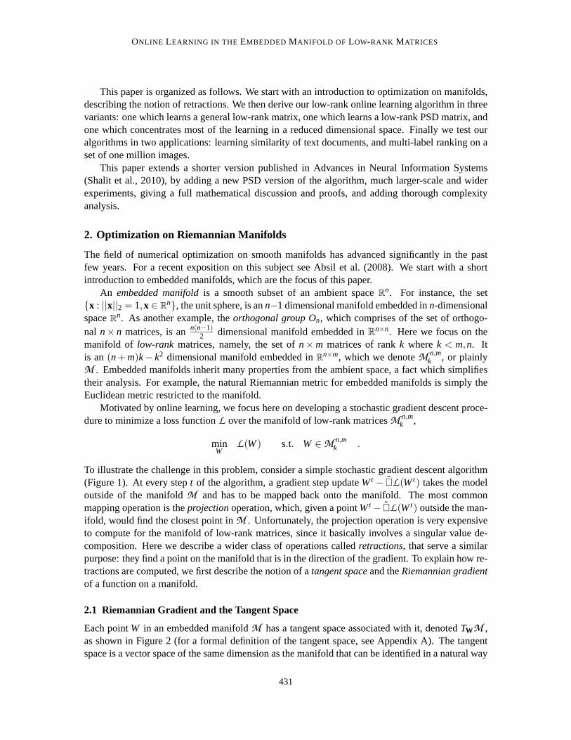
This paper is organized as follows. We start with an introduction to optimization on manifolds,describing the notion of retractions. We then derive our low-rank online learning algorithm in threevariants: one which learns a general low-rank matrix, one which learns alow-rank PSD matrix, andone which concentrates most of the learning in a reduced dimensional space. Finally we test ouralgorithms in two applications: learning similarity of text documents, and multi-label ranking on aset of one million images.

This paper extends a shorter version published in Advances in Neural Information Systems(Shalit et al., 2010), by adding a new PSD version of the algorithm, much larger-scale and widerexperiments, giving a full mathematical discussion and proofs, and addingthorough complexityanalysis.

2. Optimization on Riemannian Manifolds

The field of numerical optimization on smooth manifolds has advanced significantly in the pastfew years. For a recent exposition on this subject see Absil et al. (2008). We start with a shortintroduction to embedded manifolds, which are the focus of this paper.

An embedded manifoldis a smooth subset of an ambient spaceRn. For instance, the set

{x : ||x||2 = 1,x ∈ Rn}, the unit sphere, is ann−1 dimensional manifold embedded inn-dimensional

spaceRn. As another example, theorthogonal group On, which comprises of the set of orthogo-nal n× n matrices, is ann(n−1)

2 dimensional manifold embedded inRn×n. Here we focus on themanifold of low-rank matrices, namely, the set ofn×m matrices of rankk wherek < m,n. Itis an(n+m)k− k2 dimensional manifold embedded inRn×m, which we denoteM n,m

k , or plainlyM . Embedded manifolds inherit many properties from the ambient space, a fact which simplifiestheir analysis. For example, the natural Riemannian metric for embedded manifolds is simply theEuclidean metric restricted to the manifold.

Motivated by online learning, we focus here on developing a stochastic gradient descent proce-dure to minimize a loss functionL over the manifold of low-rank matricesM n,m

k ,

minW

L(W) s.t. W ∈M n,mk .

To illustrate the challenge in this problem, consider a simple stochastic gradient descent algorithm(Figure 1). At every stept of the algorithm, a gradient step updateWt − ∇L(Wt) takes the modeloutside of the manifoldM and has to be mapped back onto the manifold. The most commonmapping operation is theprojectionoperation, which, given a pointWt− ∇L(Wt) outside the man-ifold, would find the closest point inM . Unfortunately, the projection operation is very expensiveto compute for the manifold of low-rank matrices, since it basically involves a singular value de-composition. Here we describe a wider class of operations calledretractions, that serve a similarpurpose: they find a point on the manifold that is in the direction of the gradient. To explain how re-tractions are computed, we first describe the notion of atangent spaceand theRiemannian gradientof a function on a manifold.

2.1 Riemannian Gradient and the Tangent Space

Each pointW in an embedded manifoldM has a tangent space associated with it, denotedTWM ,as shown in Figure 2 (for a formal definition of the tangent space, see Appendix A). The tangentspace is a vector space of the same dimension as the manifold that can be identified in a natural way

431


Figure 1: Projection onto the manifold is just a particular case of a retraction.Retractions aredefined as operators that approximate the geodesic gradient flow on the manifold.

with a linear subspace of the ambient space. It is usually simple to compute the linear projectionPW

of any point in the ambient space onto the tangent spaceTWM .

Given a manifoldM and a differentiable functionL :M →R, theRiemannian gradient∇L(W)of L onM at a pointW is a vector in the tangent spaceTWM . A very useful property of embeddedmanifolds is the following: given a differentiable functionf defined on the ambient space (and thuson the manifold), the Riemannian gradient off at pointW is simply the linear projectionPW of theEuclidean gradient off onto the tangent spaceTWM .

Thus, if we denote the Euclidean gradient ofL in Rn×m by ∇L , we have∇L(W) =PW(∇L). An

important consequence follows in case the manifold represents the set of points obeying a certainconstraint. In this case the Riemannian gradient off is equivalent to the Euclidean gradient offminus the component which is normal to the constraint. Indeed this normal component is exactlythe component which is irrelevant when performing constrained optimization.

The Riemannian gradient allows us to computeWt+ 12 =Wt−ηt∇L(W), for a given iterate point

Wt and step sizeηt . We now examine howWt+ 12 can be mapped back onto the manifold.

2.2 Retractions

Intuitively, retractionscapture the notion of "going along a straight line" on the manifold. The math-ematically ideal retraction is called theexponential mapping(Do Carmo, 1992, Chapter 3): it mapsthe tangent vectorξ ∈ TWM to a point along a geodesic curve which goes throughW in the direc-tion of ξ Figure 1. Unfortunately, for many manifolds (including the low-rank manifoldconsideredhere) calculating the geodesic curve is computationally expensive (Vandereycken et al., 2009). Amajor insight from the field of Riemannian manifold optimization is that one can use retractionswhich merely approximate the exponential mapping. Using such retractions maintains the conver-

432


gence properties obtained with the exponential mapping, but is much cheaper computationally for asuitable choice of mapping.

Definition 1 Given a point W in an embedded manifoldM , a retraction is any function RW :TWM →M which satisfies the following two conditions (Absil et al., 2008, Chapter 4):

1. Centering: RW(0) =W.

2. Local rigidity: The curveγ : (−ε,ε)→M defined byγξ(τ) = RW(τξ) satisfiesγξ(0) = ξ, whereγ is the derivative ofγ by τ.

It can be shown that any such retraction approximates the exponential mapping to a first or-der (Absil et al., 2008).Second-order retractions, which approximate the exponential mapping tosecond order aroundW, have to satisfy in addition the following stricter condition:

PW

(

dRW(τξ)dτ2 |τ=0

)

= 0,

for all ξ ∈ TWM , wherePW is thelinear projection from the ambient space onto the tangent spaceTWM . When viewed intrinsically, the curveRW(τξ) defined by a second-order retraction has zeroacceleration at pointW, namely, its second order derivatives are all normal to the manifold. The bestknown example of a second-order retraction onto embedded manifolds is theprojection operation(Absil and Malick, 2010), which maps a pointX to the pointY ∈M which is closest to it in theFrobenius norm. That is, the projection ofX ontoM is simply:

Pro jM (X) = argminY∈M

‖X−Y‖Fro

Importantly, such projections are viewed here as one type of a second order approximation to theexponential mapping, which can be replaced by any other second-order retractions, when computingthe projection is too costly (see Figure 1).

Given the tangent space and a retraction, we now define a Riemannian gradient descent proce-dure for the lossL at pointWt ∈M . Conceptually, the procedure has three steps (Figure 2):

1. Step 1: Ambient gradient: Obtain the Euclidean gradient∇L(Wt) in the ambient space.

2. Step 2: Riemannian gradient:Linearly project the ambient gradient onto the tangent spaceTWM . Computeξt = PWt (∇L(Wt)).

3. Step 3: Retraction: Retract the Riemannian gradientξt back to the manifold:Wt+1 =RWt (ξt).

With a proper choice of step size, this procedure can be proved to have local convergence forany retraction (Absil et al., 2008). In practice, the algorithm merges thesethree steps for efficiency,as discussed in the next section.

433


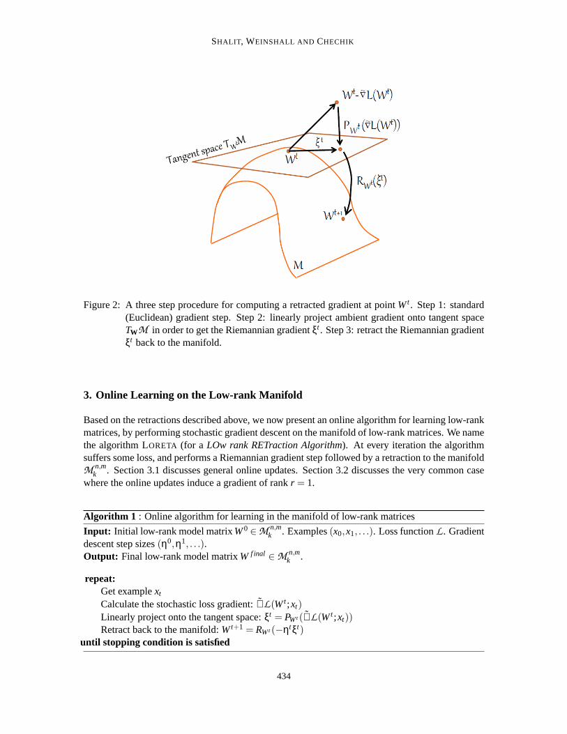
Figure 2: A three step procedure for computing a retracted gradient at point Wt . Step 1: standard(Euclidean) gradient step. Step 2: linearly project ambient gradient ontotangent spaceTWM in order to get the Riemannian gradientξt . Step 3: retract the Riemannian gradientξt back to the manifold.

3. Online Learning on the Low-rank Manifold

Based on the retractions described above, we now present an online algorithm for learning low-rankmatrices, by performing stochastic gradient descent on the manifold of low-rank matrices. We namethe algorithm LORETA (for a LOw rank RETraction Algorithm). At every iteration the algorithmsuffers some loss, and performs a Riemannian gradient step followed by aretraction to the manifoldM

n,mk . Section 3.1 discusses general online updates. Section 3.2 discusses thevery common case

where the online updates induce a gradient of rankr = 1.

Algorithm 1 : Online algorithm for learning in the manifold of low-rank matrices

Input: Initial low-rank model matrixW0∈M n,mk . Examples(x0,x1, . . .). Loss functionL . Gradient

descent step sizes(η0,η1, . . .).Output: Final low-rank model matrixW f inal ∈M n,m

k .

repeat:Get examplext

Calculate the stochastic loss gradient:∇L(Wt ;xt)

Linearly project onto the tangent space:ξt = PWt (∇L(Wt ;xt))Retract back to the manifold:Wt+1 = RWt (−ηtξt)

until stopping condition is satisfied

434


In what follows, lowercase Greek letters likeξ denote an abstract tangent vector, and uppercaseRoman letters likeA denote concrete matrix representations as kept in memory (takingn×m floatnumbers to store). We intermix the two notations, as inξ = AZ, when the meaning is clear from thecontext. The set ofn×k matrices of rankk is denotedRn×k

∗ .

3.1 The General-Rank LORETA Algorithm

In online learning we are repeatedly given a rank-r gradient matrixZ = ∇LW, and want to computea step onM n,m

k in the direction ofZ. As a first step we find its linear projection onto the tangentspaceZ = PW(Z).

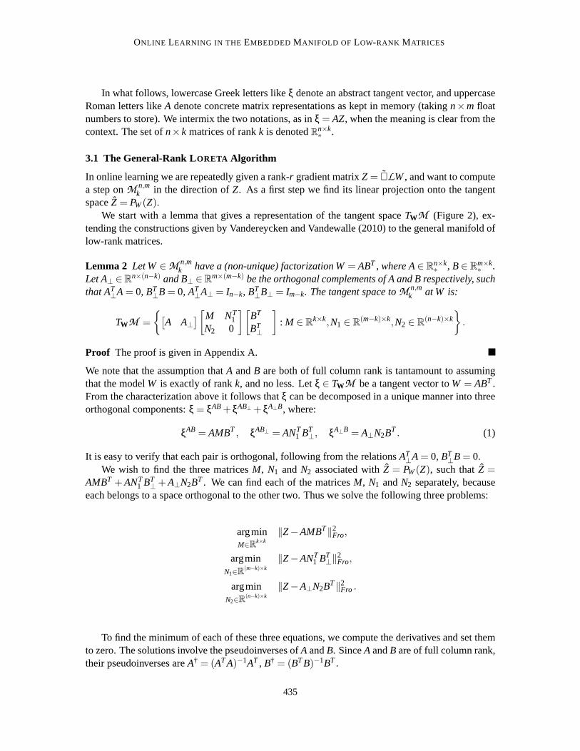
We start with a lemma that gives a representation of the tangent spaceTWM (Figure 2), ex-tending the constructions given by Vandereycken and Vandewalle (2010) to the general manifold oflow-rank matrices.

Lemma 2 Let W∈M n,mk have a (non-unique) factorization W= ABT , where A∈R

n×k∗ , B∈R

m×k∗ .

Let A⊥ ∈Rn×(n−k) and B⊥ ∈Rm×(m−k) be the orthogonal complements of A and B respectively, suchthat AT

⊥A= 0, BT⊥B= 0, AT

⊥A⊥ = In−k, BT⊥B⊥ = Im−k. The tangent space toM n,m

k at W is:

TWM =

{

[

A A⊥]

[

M NT1

N2 0

][

BT

BT⊥

]

: M ∈ Rk×k,N1 ∈ R

(m−k)×k,N2 ∈ R(n−k)×k

}

.

Proof The proof is given in Appendix A.

We note that the assumption thatA andB are both of full column rank is tantamount to assumingthat the modelW is exactly of rankk, and no less. Letξ ∈ TWM be a tangent vector toW = ABT .From the characterization above it follows thatξ can be decomposed in a unique manner into threeorthogonal components:ξ = ξAB+ξAB⊥+ξA⊥B, where:

ξAB = AMBT , ξAB⊥ = ANT1 BT⊥, ξA⊥B = A⊥N2BT . (1)

It is easy to verify that each pair is orthogonal, following from the relationsAT⊥A= 0, BT

⊥B= 0.We wish to find the three matricesM, N1 andN2 associated withZ = PW(Z), such thatZ =

AMBT +ANT1 BT⊥+A⊥N2BT . We can find each of the matricesM, N1 andN2 separately, because

each belongs to a space orthogonal to the other two. Thus we solve the following three problems:

argminM∈R

k×k

‖Z−AMBT‖2Fro,

argminN1∈R

(m−k)×k

‖Z−ANT1 BT⊥‖

2Fro,

argminN2∈R

(n−k)×k

‖Z−A⊥N2BT‖2Fro .

To find the minimum of each of these three equations, we compute the derivatives and set themto zero. The solutions involve the pseudoinverses ofA andB. SinceA andB are of full column rank,their pseudoinverses areA† = (ATA)−1AT , B† = (BTB)−1BT .

435


M = (ATA)−1ATZB(BTB)−1 = A†ZB†T, (2)

N1 = BT⊥ZTA(ATA)−1 = BT

⊥ZTA†,

N2 = AT⊥ZB(BTB)−1 = AT

⊥ZB†T.

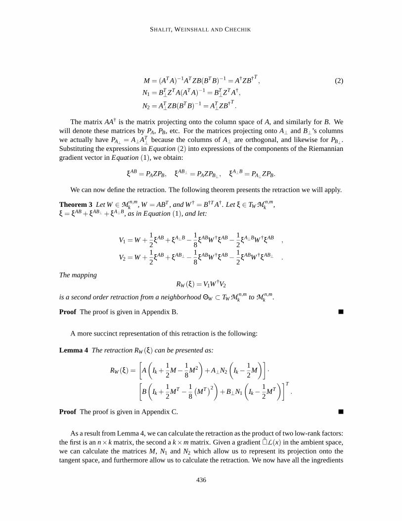
The matrixAA† is the matrix projecting onto the column space ofA, and similarly forB. Wewill denote these matrices byPA, PB, etc. For the matrices projecting ontoA⊥ andB⊥’s columnswe actually havePA⊥ = A⊥AT

⊥ because the columns ofA⊥ are orthogonal, and likewise forPB⊥ .Substituting the expressions inEquation(2) into expressions of the components of the Riemanniangradient vector inEquation(1), we obtain:

ξAB = PAZPB, ξAB⊥ = PAZPB⊥ , ξA⊥B = PA⊥ZPB.

We can now define the retraction. The following theorem presents the retraction we will apply.

Theorem 3 Let W∈M n,mk , W = ABT , and W† = B†TA†. Letξ ∈ TWM

n,mk ,

ξ = ξAB+ξAB⊥+ξA⊥B, as in Equation(1), and let:

V1 =W+12

ξAB+ξA⊥B−18

ξABW†ξAB−12

ξA⊥BW†ξAB ,

V2 =W+12

ξAB+ξAB⊥−18

ξABW†ξAB−12

ξABW†ξAB⊥ .

The mappingRW(ξ) =V1W

†V2

is a second order retraction from a neighborhoodΘW ⊂ TWMn,mk toM n,m

k .

Proof The proof is given in Appendix B.

A more succinct representation of this retraction is the following:

Lemma 4 The retraction RW(ξ) can be presented as:

RW(ξ) =[

A

(

Ik+12

M−18

M2)

+A⊥N2

(

Ik−12

M

)]

·

[

B

(

Ik+12

MT −18

(

MT)2)

+B⊥N1

(

Ik−12

MT)]T

.

Proof The proof is given in Appendix C.

As a result from Lemma 4, we can calculate the retraction as the product of two low-rank factors:the first is ann×k matrix, the second ak×mmatrix. Given a gradient∇L(x) in the ambient space,we can calculate the matricesM, N1 and N2 which allow us to represent its projection onto thetangent space, and furthermore allow us to calculate the retraction. We nowhave all the ingredients

436


Algorithm 2 : Naive Riemannian stochastic gradient descent

Input: Matrices A ∈ Rn×k∗ , B ∈ R

m×k∗ s.t. W = ABT . Gradient matrixG ∈ R

n×m s.t.G = −η∇L(W) ∈ R

n×m, where ∇L(W) is the gradient in the ambient space andη > 0 isthe step size.

Output: MatricesZ1 ∈ Rn×k∗ , Z2 ∈ R

m×k∗ such thatZ1ZT

2 = RW(−η∇L(W)).

Compute: matrix dimensionA† = (ATA)−1AT , B† = (BTB)−1BT k×n, k×mA⊥, B⊥= orthogonal complements ofA,B n× (n−k), m× (m−k)M = A†GB†T k×kN1 = BT

⊥GTA†T (m−k)×kN2 = AT

⊥GB†T (n−k)×kZ1 = A

(

Ik+ 12M− 1

8M2)

+A⊥N2(

Ik− 12M

)

n×kZ2 = B

(

Ik+ 12MT − 1

8(MT)2

)

+B⊥N1(

Ik− 12MT

)

m×k

necessary for a Riemannian stochastic gradient descent algorithm. The procedure is outlined inAlgorithm 2.

Algorithm 2 explicitly computes and stores the orthogonal complement matricesA⊥ andB⊥,which in the low rank casek≪ m,n, have sizeO(mn), the same as the full sizedW. To improvethe memory complexity, we use the fact that the matricesA⊥ and B⊥ always operate with theirtranspose. SinceA⊥ andB⊥ have orthogonal columns, the matrixA⊥AT

⊥ is actually the projectionmatrix that we denoted earlier byPA⊥ , and likewise forB⊥. Because of orthogonal complementarity,these projection matrices are equal toIn−PA andIm−PB respectively. Thus we can writeA⊥N2 =(

I −AA†)

ZB†T, and a similar identity forB⊥N1.

Consider now the case where the gradient matrix is of rank-r and is available in a factorizedform Z = G1GT

2 , with G1 ∈ Rn×r , G2 ∈ R

m×r . Using the factorized gradient we can reformulate thealgorithm to keep in memory only matrices of size at most max(n,m)×k or max(n,m)× r. Optimiz-ing the order of matrix operations so that the number of operations is minimized gives Algorithm3. The runtime complexity of Algorithm 3 is readily computed based on matrix multiplicationscomplexity,2 and isO

(

(n+m)(k+ r)2)

.

3.2 LORETA With Rank-one Gradients

In many learning problems, the gradient matrix∇L(W) required for a gradient step update has arank of one. This is the case for example, when the matrix modelW acts as a bilinear form on twovectors,p andq, and the loss is a piecewise linear function ofpTWq (as in Grangier and Bengio,2008; Chechik et al., 2010; Weinberger and Saul, 2009; Shalev-Shwartz et al., 2004 and Section 7.1below). In that case, the gradient is the rank-one outer product matrixpqT . As another example,consider the case of multitask learning, where the matrix modelW operates on a vector inputp, andthe loss is the squared loss‖Wp−q‖2 between the multiple predictionsWp and the true labelsq.The gradient of this loss is(Wp−q)pT , which is again a rank-one matrix. We now show how to

2. We assume throughout this paper the use of ordinary (schoolbook)matrix multiplication.

437


Algorithm 3 : L ORETA -r - General-rank Riemannian stochastic gradient descent

Input: Matrices A ∈ Rn×k∗ , B ∈ R

m×k∗ s.t. W = ABT . Matrices G1 ∈ R

n×r , G2 ∈ Rm×r s.t.

G1GT2 = −η∇L(W) ∈ R

n×m, where∇L(W) is the gradient in the ambient space andη > 0 is thestep size.


m×k∗ such thatZ1ZT

2 = RW(−η∇L(W)).

Compute: matrix dimension runtime complexityA† = (ATA)−1AT , B† = (BTB)−1BT k×n, k×m O((n+m)k2)a1 = A† ·G1, b1 = B† ·G2 k× r, k× r O((n+m)kr)a2 = A·a1 n× r O(nkr)Q= b1

T ·a1 r× r O(kr2)

a3 =−12a2+

38a2 ·Q+G1−

12G1 ·Q n× r O(nr2)

Z1 = A+a3 ·b1T n×k O(nkr)

b2 =(

GT2 B

)

·B† r×m O(mkr)b3 =−

12b2+

38Q·b2+GT

2 −12Q·GT

2 r×m O(mr2)ZT

2 = BT +a1 ·b3 k×m O(mkr)

reduce the complexity of each iteration to be linear in the model rankk when the rank of the gradientmatrix isr = 1.

Algorithm 4 : L ORETA -1 - Rank-one Riemannian stochastic gradient descent

Input: MatricesA∈ Rn×k∗ , B∈ R

m×k∗ s.t. W = ABT . MatricesA† andB†, the pseudo-inverses ofA

andB respectively. Vectorsp ∈ Rn×1, q ∈ R

m×1 s.t. pqT = −η∇L(W) ∈ Rn×m, where∇L(W) is

the gradient in the ambient space andη > 0 is the step size.


m×k∗ s.t. Z1ZT

2 = RW(−η∇L(W)). MatricesZ†1 andZ†

2, thepseudo-inverses ofZ1 andZ2 respectively.

Compute: matrix dimension runtime complexitya1 = A† ·p,b1 = B† ·q k×1 O((n+m)k)a2 = A·a1 n×1 O(nk)s= b1

T ·a1 1×1 O(k)a3 = a2

(

−12 +

38s)

+p(1− 12s) n×1 O(n)

Z1 = A+a3 ·b1T n×k O(nk)

b2 =(

qTB)

·B† 1×m O(mk)b3 = b2

(

−12 +

38s)

+qT(1− 12s) 1×m O(m)

ZT2 = BT +a1 ·b3 k×m O(mk)

Z†1 = rank_one_pseudoinverse_update(A,A†,a3,b1) k×n O(nk)

Z†2 = rank_one_pseudoinverse_update(B,B†,b3,a1) k×m O(mk)

Given rank-one gradients, the most computationally demanding step in Algorithm 3 is the com-putation of the pseudo-inverse of the matricesA andB, takingO(nk2) andO(mk2) operations. Allother operations areO(max(n,m) · k) at most. To speed up calculations we use the fact that for

438


r = 1 the outputsZ1 andZ2 become rank-one updates of the input matricesA andB. This enablesus to keep the pseudo-inversesA† andB† from the previous round, and perform a rank-one updateto them, following a procedure developed by Meyer (1973). The full procedure is included in Ap-pendix D. This procedure is similar to the better known Sherman-Morrison formula for the inverseof a rank-one perturbed matrix, and its computational complexity for ann× k matrix isO(nk) op-erations. Using that procedure, we derive our final algorithm, LORETA-1, the rank-one Riemannianstochastic gradient descent. Its overall time and space complexity are bothO((n+m)k) per gradientstep. It can be seen that the LORETA-1 algorithm uses only basic matrix operations, with the mostexpensive ones being low-rank matrix-vector multiplication and low-rank matrix-matrix addition.The memory requirement of LORETA-1 is about 4nk (assumingm= n), since it receives four in-put matrices of sizenk (A,B,A†,B†) and assuming it can compute the four outputs (Z1,Z2,Z

†1,Z

†2),

in-place while destroying previously computed terms.

4. Online Learning of Low-rank Positive Semidefinite Matrices

In this section we adapt the derivation above to the special case of positive semidefinite (PSD)matrices. PSD matrices are of special interest because they encode a trueEuclidean metric. Ann-by-nPSD matrixW of rank-k can be factored asW=YYT , withY∈R

n×k. Thus, the bilinear formxTWzis equal to(Yx)T(Yz), which is a Euclidean inner product in the space spanned byY’s columns.These properties have led to an extensive use of PSD matrix models in metric and similarity learning,see, for example, Xing et al. (2002), Goldberger et al. (2005), Globerson and Roweis (2006), Bar-Hillel et al. (2006) and Jain et al. (2008). The set ofn-by-n PSD matrices of rank-k forms a manifoldof dimensionnk− k(k−1)

2 , embedded in the Euclidean spaceRn×n (Vandereycken et al., 2009). We

denote this manifold byS+(k,n).We now give a characterization of the tangent space of this manifold, due toVandereycken and

Vandewalle (2010).

Lemma 5 Let W∈ S+(k,n) have a (non-unique) factorization W= YYT , where Y∈ Rn×k∗ . Let

Y⊥ ∈ Rn×(n−k) be the orthogonal complement of Y such that YT

⊥Y = 0, YT⊥Y⊥ = In−k. The tangent

space toS+(k,n) at W is:

TWS+(k,n) =

{

[

Y Y⊥]

[

S NT

N 0

][

YT

YT⊥

]

: S∈ Rk×k,N ∈ R

(n−k)×k,S= ST}

.

Proof See Vandereycken and Vandewalle (2010), Proposition 5.2.

Let ξ∈TWS+(k,n) be a tangent vector toW=YYT . As shown by Vandereycken and Vandewalle(2010),ξ can be decomposed into two orthogonal components,ξ = ξS+ξP. Given a rank-r gradientmatrixZ, and using the projection matricesPY andPY⊥ they show that:

ξS= PYZ+ZT

2PY,

ξP = PY⊥Z+ZT

2PY +PY

Z+ZT

2PY⊥ .

Using this characterization of the tangent vector when given an ambient gradientZ, one candefine a retraction analogous to that defined in Section 3. This retraction is referred to asR(2)

W inVandereycken and Vandewalle (2010).

439


Theorem 6 Let W∈ S+(k,n), W = YYT , and W† be its pseudo-inverse. Letξ ∈ TWS+(k,n), ξ =ξS+ξP, as described above, and let

V =W+12

ξS+ξP−18

ξSW†ξS−12

ξPW†ξS.

The mapping RPSDW (ξ) =VW†V is a second order retraction from a neighborhood

ΘW ⊂ TWS+(k,n) to S+(k,n).

Proof See Vandereycken and Vandewalle (2010), Proposition 5.10.

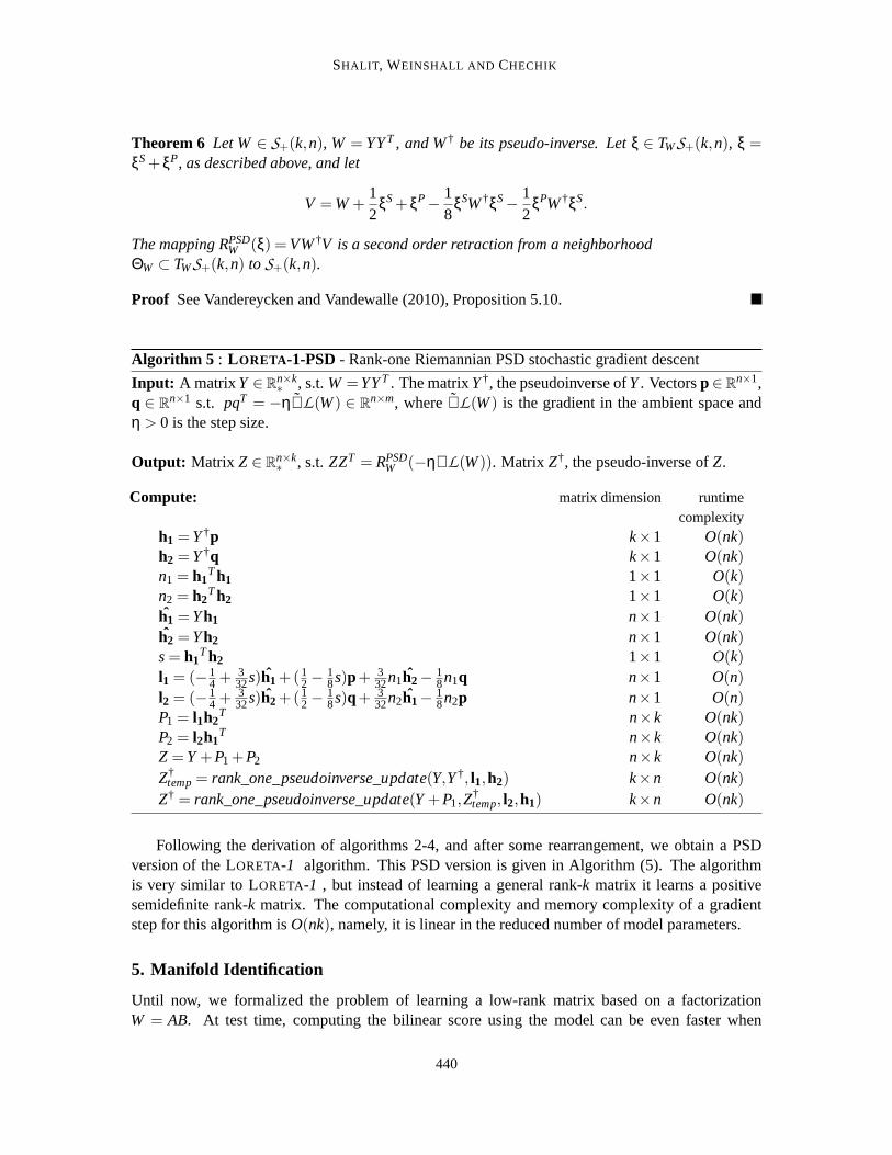
Algorithm 5 : L ORETA -1-PSD- Rank-one Riemannian PSD stochastic gradient descent

Input: A matrixY ∈Rn×k∗ , s.t.W =YYT . The matrixY†, the pseudoinverse ofY. Vectorsp∈R

n×1,q ∈ R

n×1 s.t. pqT = −η∇L(W) ∈ Rn×m, where∇L(W) is the gradient in the ambient space and

η > 0 is the step size.

Output: Matrix Z ∈ Rn×k∗ , s.t.ZZT = RPSD

W (−η∇L(W)). Matrix Z†, the pseudo-inverse ofZ.

Compute: matrix dimension runtimecomplexity

h1 =Y†p k×1 O(nk)h2 =Y†q k×1 O(nk)n1 = h1

Th1 1×1 O(k)n2 = h2

Th2 1×1 O(k)h1 =Yh1 n×1 O(nk)h2 =Yh2 n×1 O(nk)s= h1

Th2 1×1 O(k)l1 = (−1

4 +332s)h1+(1

2−18s)p+ 3

32n1h2−18n1q n×1 O(n)

l2 = (−14 +

332s)h2+(1

2−18s)q+ 3

32n2h1−18n2p n×1 O(n)

P1 = l1h2T n×k O(nk)

P2 = l2h1T n×k O(nk)

Z =Y+P1+P2 n×k O(nk)Z†

temp= rank_one_pseudoinverse_update(Y,Y†, l1,h2) k×n O(nk)Z† = rank_one_pseudoinverse_update(Y+P1,Z

†temp, l2,h1) k×n O(nk)

Following the derivation of algorithms 2-4, and after some rearrangement, we obtain a PSDversion of the LORETA-1 algorithm. This PSD version is given in Algorithm (5). The algorithmis very similar to LORETA-1 , but instead of learning a general rank-k matrix it learns a positivesemidefinite rank-k matrix. The computational complexity and memory complexity of a gradientstep for this algorithm isO(nk), namely, it is linear in the reduced number of model parameters.

5. Manifold Identification

Until now, we formalized the problem of learning a low-rank matrix based on afactorizationW = AB. At test time, computing the bilinear score using the model can be even faster when

440


the data is sparse. For instance, given two vectorsx1 andx2 with c1 andc2 non-zero values, com-puting the bilinear formxT

1 ABTx2 requiresO(c1k+k+kc2) = O((c1+c2)k) operations, and can besignificantly faster than the dense case. However, at training time, the LORETA-1 algorithm still hasa complexity ofO((m+n)k) for each iteration even when the data is sparse.

The current section describes an attempt to adapt LORETA-1 such that it treats sparse data moreefficiently. The empirical evaluation of this adaptation showed mixed results, but we include thederivation for completeness. The main idea is to separate the low-rank projection into two steps.First, a projection to a low dimensional spaceAx that can be computed efficiently whenx is sparse.Then, learning a second matrix, whose role is to tune the representation in thek-dimensional space.

To explain the idea, we focus on the case of learning a low-rank model which parametrizesa similarity function. The model isW = ABT , A ∈ R

n×k, B ∈ Rn×k. The similarity between two

vectorsp,q ∈ Rn is then given by

Sim(p,q) = pTWq = (ATp)T · (BTq). (3)

This similarity measure can be viewed as the cosine similarity inRk between the projected vectors

BTq andATp. We now introduce another similarity model which operates directly in the projectedspace. Formally, we haveM ∈ R

k×k, and the similarity model is

Sim(p,q) = (ATp)TM(BTq) = pTAMBTq. (4)

Clearly, since the model in Equation (4) involves only linear matrix multiplications, itsdescrip-tive power is equivalent to that of the model Equation (3). However, it has the potential to belearned faster. To speed the training we can iterate between learning the outer projections A,B us-ing LORETA , and learning the inner low-dimensional similarity modelM using standard methodsoperating in the low-dimensional space. Specifically, the idea is to executes update steps ofM forevery update step ofA,B (Algorithm 6). Afters update steps toM, it is decomposed using SVD toobtainM =USVT , and these factors are used to update the outer projections usingA← AUsqrt(S),B← BVsqrt(S).

Consider the computational complexity: Given two sparse vectorsx1, x2 with c1 andc2 non-zerovalues respectively, projecting them usingA andB to the low dimensional space takesO(k(c1+c2)),and an update step of M takesO(k2). DecomposingM using SVD takesO(k3), so the overallcomplexity fors updates isO

(

k ·(

s(k+c1+c2)+k2))

. Whens≥ k the cost of decomposition isamortized across manyM updates and does not increase the overall complexity. The update ofA, BtakesO(k(n+m)) as before. This approach is related to the idea of manifold identification (Oberlinand Wright, 2007), where the learning ofA, B "identifies" a manifold of rankk and the inner stepsoperate to tune the representation within that subspace.

This iterative procedure could be a significant speed up compared to the original O((m+n)k).Unfortunately, when we tested this algorithm in a similarity learning task (as in Section 7.1), itsperformance was not as good as that of LORETA-1. The main reason was numerical instability:The matrixM typically collapsed to match few directions inA, and decomposing it has amplifiedthe sameA directions. This approach awaits deeper investigation which is outside the scope of thecurrent paper.

6. Related Work

A recent summary of many advances in the field of optimization on manifolds is given by Absilet al. (2008). Advances in this field have lately been applied to matrix completion(Keshavan et al.,

441


Algorithm 6 : Manifold identification meta-algorithm

Input: Initial model matricesA ∈ Rn×k∗ , B ∈ R

m×k∗ s.t. W = ABT . MatricesA† and B†, the

pseudo-inverses ofA andB respectively. Loss functionL .Output: MatricesA∈ R

n×k∗ , B∈ R

m×k∗ s.t.W = ABT .

Parameters: η1: LORETA step size .η2: low-dimensional similarity learning step size.s: numberof low-dimensional learning steps per round

repeat:[g1,g2] = ∇L(ABT)[A,B,A†,B†] = LORETA

(

A,B,A†,B†,g1,g2,η1)

initialize M = Ikfor i=1:s

[g1,g2] = ∇L(AMBT)M = f ull − rank−metric− learning

(

M,ATg1,BTg2,η2)

endfor[U,S,V] = svd(M)A= A·U ·sqrt(S)B= B·V ·sqrt(S)

until stopping condition is satisfied

2010), tensor-rank estimation (Eldén and Savas, 2009; Ishteva et al., 2011) and sparse PCA (Journéeet al., 2010b).

Broadly speaking, there are two kinds of manifolds used in optimization. The first areembeddedmanifolds, manifolds that form a subset of Euclidean space, and are the ones we employ in this work.The second kind arequotient manifolds, which are formed by defining an equivalence relation ona Euclidean space, and endowing the resulting equivalence classes with an appropriate Riemannianmetric. For example, the equivalence relation onR

n defined byx∼ y ⇐⇒ ∃λ > 0, x= λy, yields aquotient space called thereal projective spacewhen given a proper Riemannian metric.

More specific to the field of low-rank matrix manifolds, work has been done on the generalproblem of optimization with low-rank positive semi-definite (PSD) matrices. Thelatest and mostrelevant is the work of Meyer et al. (2011). In this work, Meyer and colleagues develop a frameworkfor Riemannian stochastic gradient descent on the manifold of PSD matrices,and apply it to theproblem of kernel learning and the learning of Mahalanobis distances. Their main technical tool isthat of quotient manifolds mentioned above, as opposed to the embedded manifold we use in thiswork. Another paper which uses a quotient manifold representation is thatof Journée et al. (2010a),which introduces a method for optimizing over low-rank PSD matrices.

In their 2010 paper (Vandereycken and Vandewalle, 2010), Vandereycken et al. introduced aretraction for PSD matrices in the context of modeling systems of partial differential equations. Webuild on this work in order to construct our methods of learning general and PSD low-rank matrices.

In general, the problem of minimizing a convex function over the set of low-rank matrices wasaddressed by several authors, including Fazel (2002). Recht et al. (2010) and more recently Jainet al. (2011) also consider the same problem, with additional affine constraints, and its connectionto recent advances in compressed sensing. The main tools used in these papers are the trace norm

442


(sum of singular values) and semi-definite programming. See also Fazel etal. (2005) for a shortintroduction to these methods.

More closely related to the current paper are the papers by Kulis et al. (2009) and Meka et al.(2008). Kulis et al. (2009) deal with learning low-rank PSD matrices, anduse the rank-preservinglog-det divergence and clever factorization and optimization in order to derive an update rule withruntime complexity ofO(nk2) for ann×n matrix of rankk. Meka et al. (2008) use online learningin order to find a minimal rank square matrix under approximate affine constraints. The algorithmdoes not directly allow a factorized representation, and depends on an "oracle" component, whichtypically requires to compute an SVD.

Multi-class ranking with a large number of features was studied by Bai et al.(2009), and in thecontext of factored representations, by Weston et al. (2011) (WSABIE). WSABIE combines pro-jected gradient updates with a novel sampling scheme which is designed to minimizea ranking lossnamed WARP. WARP is shown to outperform simpler triplet sampling approaches. Since WARPyields rank-1 gradients, it can easily be adapted for Riemannian SGD, butwe leave experimentswith such sampling schemes to future work.

7. Experiments

We tested LORETA in two learning tasks: learning a similarity measure between pairs of text doc-uments using the 20-newsgroups data collected by Lang (1995), and learning to rank image labelannotations based on a multi-label annotated set, using theImageNetdata set (Deng et al., 2009).Matlab code for LORETA-1 is available online athttp://chechiklab.biu.ac.il/research/LORETA.

7.1 Learning Similarity on the 20 Newsgroups Data Set

In our first set of experiments, we looked at the problem of learning a similarity measure betweenpairs of text documents. Similarity learning is a well studied problem, closely related to metriclearning (see Yang 2007 for a review). It has numerous applications in information retrieval such asquery by example, and finding related content on the web.

One approach to learn pairwise relations is to measure the similarity of two documentsp,q∈Rn

using a bilinear form parametrized by a modelW ∈ Rn×n:

SW(p,q) = pTWq.

Such models can be learned online (Chechik et al., 2010) and were shownto achieve high precision.Sometimes the matrixW is required to be symmetric and positive definite, which means it actuallyencodes a metric, also known as a Mahalanobis distance. Unfortunately, since the number of param-eters grows asn2, storing the matrixW in memory is only feasible for limited feature dimensionality.To handle larger vocabularies, like those containing all textual terms foundin a corpus, a commonapproach is to pre-select a subset of the features and train a model over the low dimensional data.However, such preprocessing may remove crucial signals in the data even if features are selected ina discriminative way.

To overcome this difficulty, we used LORETA-1 and LORETA-1-PSD to learn a rank-k parametriza-tion of the modelW. This model can be factorized asW = ABT , whereA,B∈ R

n×k for the generalcase, or asW = AAT for the PSD case. In each of our experiments, we selected a subset ofn fea-tures, and trained a rankk model. We varied the number of featuresn and the rank of the matrixk

443


so as to use a fixed amount of memory. For example, we used a rank-10 model with 50K features,and a rank-50 model with 10K features.

7.1.1 SIMILARITY LEARNING WITH LORETA-1

We use an online procedure similar to that in Grangier and Bengio (2008) and Chechik et al. (2010).At each round, three instances are sampled: a query documentq∈R

n, and two documentsp+, p− ∈R

n such thatp+ is known to be more similar toq thanp−. We wish that the model assigns a highersimilarity score to the pair(q,p+) than the pair(q,p−), and hence use the online ranking hinge lossdefined aslW(q,p+,p−) = [1−SW(q,p+)+SW(q,p−)]+, where[z]+ = max(z,0).

We initialized the model to be a truncated identity matrix, with only the firstk ones along thediagonal. This corresponds in our case to choosing thek most informative terms as the initial dataprojection.

7.1.2 DATA PREPROCESSING ANDFEATURE SELECTION

We used the 20 newsgroups data set (people.csail.mit.edu/jrennie/20Newsgroups), containing 20classes with approximately 1000 documents each. We removed stop words but did not apply stem-ming. The document terms form a vocabulary of 50,000 terms, and we selected a subset of thesefeatures that conveyed high information about the identity of the class (over the training set) usingthe infogaincriterion (Yang and Pedersen, 1997). This is a discriminative criterion,which measuresthe number of bits gained for category prediction by knowing the presenceor absence of a term in adocument. The selected features were normalized usingtf-idf, and then represented each documentas a bag of words. Two documents were considered similar if they shared the same class label, outof the possible 20 labels.

7.1.3 EXPERIMENTAL PROCEDURE ANDEVALUATION PROTOCOL

The 20 newsgroups site proposes a split of the data into train and test sets.We repeated splitting 5times based on the sizes of the proposed splits (a train / test ratio of 65% / 35%). We evaluated thelearned similarity measures using a ranking criterion. We view every document q in the test set as aquery, and rank the remaining test documentsp by their similarity scoresqTWp. We then computethe precision (fraction of positives) at the topr ranked documents. We then average the precisionover all positionsr such that there exists a positive example in the topr. This final measure is calledmean average precision, and is commonly used in the information retrieval community (Manninget al., 2008, Chapter 8).

7.1.4 COMPARISONS

We compared LORETA with the following approaches.

1. Naive gradient descent(GD): similar to Bai et al. (2009). The model is represented as aproduct of two matricesW = ABT . Stochastic gradient descent steps are computed over thefactorsA andB, for the same loss used by LORETA lW(q,p+,p−). The GD steps are:

Anew= A−ηq(p−−p+)TB,

Bnew= B−η(p−−p+)qTA.

We found this approach to be very unstable, and thus its results are not presented.

444


2. Naive PSD gradient descent: similar to the method above, except that now the model is con-strained to be PSD. The model is represented as a productW = AAT . Stochastic gradient de-scent steps are computed over the factorA for the same loss used by LORETA : lW(q,p+,p−).As shown by Meyer et al. (2011), this is in fact equivalent to Riemannian stochastic GD in themanifold of PSD matrices when this manifold is endowed with a certain metric the authorscall theflat metric.

The GD step is:

Anew= A−η(

q(p−−p+)T +(p−−p+)qT)A.

The step sizeη was chosen by cross validation. This approach was more stable in the PSDcase than in the general case, probably because the invariant space here is only the groupof orthogonal matrices (which are well-conditioned), as opposed to the group of invertiblematrices which might be ill-conditioned.

3. Iterative Passive-Aggressive (PA): since we found the above general GD procedure(1) to bevery unstable, we experimented with a related online algorithm from the family ofpassive-aggressive algorithms (Crammer et al., 2006). We iteratively optimize overA given a fixedBand vice versa. The optimization is a tradeoff between minimizing the losslW, and limitinghow much the models change at each iteration. The steps sizes for updatingA andB arecomputed to be:

ηA = min

(

lW(q,p+,p−)‖q‖2 · ‖BT(p+−p−)‖2

,C

)

,

ηB = min

(

lW(q,p+,p−)‖(p+−p−)‖2 · ‖ATq‖2

,C

)

.

C is a predefined parameter controlling the maximum magnitude of the step size, chosen bycross-validation. This procedure is numerically more stable because of thenormalization bythe norms of the matrices multiplied by the gradient factors.

4. Full rank similarity learning models. We compared with two full rank online metric learn-ing methods, LEGO (Jain et al., 2008) and OASIS (Chechik et al., 2010). Both algorithmslearn a full (non-factorized) model, and were run withn = 1000, in order to be consistentwith the memory constraint of LORETA-1. We have also compared with both full-rank mod-els using rank 2000, that is, 4 times the memory constraint. We have not compared with batchapproaches such as Kulis et al. (2009), since they are not expected toscale to very large datasets such as those our work is ultimately aiming towards.

In addition, we have experimented with the method for learning PSD matrices using a polargeometry characterization of the quotient manifold, due to Meyer et al. (2011). This method’sruntime complexity isO((n+m)k2), and we have found that its performance was not in line withthe methods described above.

7.1.5 RESULTS

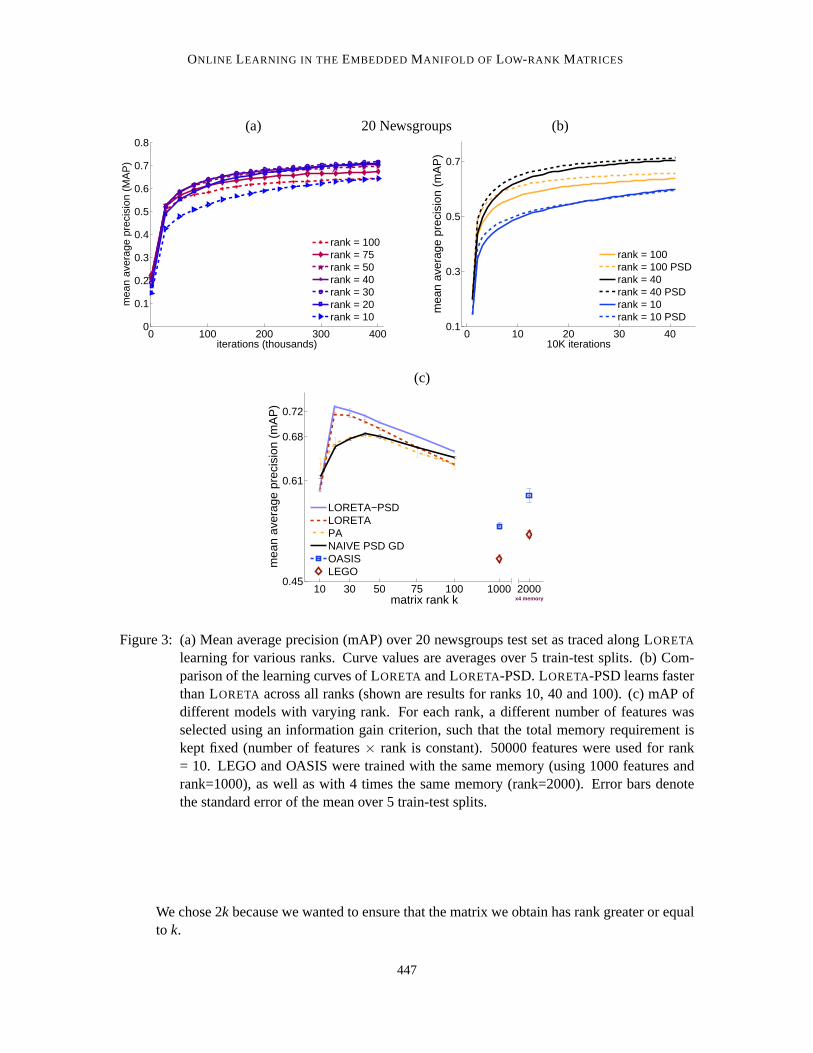
Figure 3c shows the mean average precision obtained with all the above methods. LORETA out-performs the other approaches across all ranks. LORETA-PSD achieves slightly higher precision

445


than LORETA. The reason may be that similarity was defined based on two samples belongingtoa common class, and this relation is symmetric and transitive, two relations which are respectedby PSD matrices but not by general similarity matrices. Moreover, LORETA-PSD learned fasteralong the training iterations when compared with LORETA - see Figure 3a for a comparison of thelearning curves. Interestingly, for both LORETA algorithms learning a low-rank model of rank 30,using the best 16660 features, was significantly more precise than learning a much fuller model ofrank 100 and 5000 features, or a model using the full 50000 word vocabulary but with rank 10 . Theintuition is that LORETA can be viewed as adaptively learning a linear projection of the data intolow dimensional space, which is tailored to the pairwise similarity task.

7.2 Image Multilabel Ranking

Our second set of experiments tackled the problem of learning to rank labels for images taken froma large number of classes(L = 1660) with multiple labels per image.

In our approach, we learn a linear classifier overn features for each labelc∈ C = {1, . . . ,L},and stack all models together to a single matrixW ∈ R

L×n. At test time, given an imagep ∈ Rn,

the productWp provides scores for every label for that imagep. Given ground truth labeling, agood model would rank the true labels higher than the false ones. Each rowof the matrix model canbe thought of as a sub-model for the corresponding label. Imposing a low-rank constraint on themodel implies that these sub-models are linear combinations of a smaller number oflatent models.Alternatively, we can view learning a factored rank-k modelW = ABT as learning a projection andclassifier in the projected space concurrently. The matrixBT projects the data onto ak dimensionalspace, and the matrixA consists ofL classifiers operating in the low-dimensional space. The datawe used for the experiment had∼1500 labels, but the full ImageNet data set currently has∼15000labels, and is growing.

7.2.1 ONLINE LEARNING OF LABEL RANKINGS WITH LORETA-1

At each iteration, an imagep is sampled, and using the current modelW the scores for all its labelsare computed,Wp. These scores are compared with the ground truth labelingy = {y1, . . . ,yr} ⊂ C .We wish for all the scores of the true labels to be higher than the scores forthe other labels bya margin of 1. Thus, the learner suffers a multilabel multiclass hinge loss as follows. Let y =argmaxs/∈y(Wp)s, be the negative label which obtained the highest score, where(Wp)s is thesth

component of the score vectorWp.The loss is thenL(W,p,y) = ∑r

i=1 [(Wp)y− (Wp)yi +1]+, which is the sum of the marginsbetween the top-ranked false label and all the positive labels which violatedthe margin of one fromit. We used the subgradientG of this loss for LORETA: for the set of indicesi1, i2, . . . id ⊂ y whichincurred a non zero hinge loss, thei j row of G is p, and for the row ¯y G is−d ·p. The matrixG isrank one, unless no loss was suffered in which case it is 0.

The non-convex and stochastic nature of the learning procedure has lead us to try several initialconditions:

• Zero matrix : in this initialization we begin with a low-rank matrix composed entirely ofzeros. This matrix is not included in the low-rank manifoldM n,m

k , since its rank is less thank. We therefore perform a simple pre-training session in which we add up subgradients untila matrix of rankk is obtained. In practice we added the first 2k subgradients (each suchsubgradient being of rank one), and then performed an SVD to obtain thebest rank-k model.

446


(a) 20 Newsgroups (b)

0 100 200 300 4000

0.1

0.2

0.3

0.4

0.5

0.6

0.7

0.8

iterations (thousands)

mea

n av

erag

e pr

ecis

ion

(MA

P)

rank = 100rank = 75rank = 50rank = 40rank = 30rank = 20rank = 10

0 10 20 30 400.1

0.3

0.5

0.7

10K iterations

mea

n av

erag

e pr

ecis

ion

(mA

P)

rank = 100rank = 100 PSDrank = 40rank = 40 PSDrank = 10rank = 10 PSD

(c)

10 30 50 75 100 1000 20000.45

0.61

0.68

0.72

matrix rank k

mea

n av

erag

e pr

ecis

ion

(mA

P)

LORETA−PSDLORETAPANAIVE PSD GDOASISLEGO

x4 memory

Figure 3: (a) Mean average precision (mAP) over 20 newsgroups testset as traced along LORETA

learning for various ranks. Curve values are averages over 5 train-test splits. (b) Com-parison of the learning curves of LORETA and LORETA-PSD. LORETA-PSD learns fasterthan LORETA across all ranks (shown are results for ranks 10, 40 and 100). (c)mAP ofdifferent models with varying rank. For each rank, a different numberof features wasselected using an information gain criterion, such that the total memory requirement iskept fixed (number of features× rank is constant). 50000 features were used for rank= 10. LEGO and OASIS were trained with the same memory (using 1000 features andrank=1000), as well as with 4 times the same memory (rank=2000). Error bars denotethe standard error of the mean over 5 train-test splits.

We chose 2k because we wanted to ensure that the matrix we obtain has rank greater or equalto k.

447


(a) ImageNet 50K (b) ImageNet 1M

10 50 150 250 400 10000

0.02

0.074

0.109

matrix rank k

mea

n av

erag

e pr

ecis

ion

(mA

P)

Loreta / trunc. id.Loreta−1 rand. init.Iterative PA / trunc. id.Iterative PA rand. init.Matrix PerceptronGroup MC Perceptron

10 50 150 250 400 10000

0.04

0.12

0.2

matrix rank k

mea

n av

erag

e pr

ecis

ion

(mA

P)

Loreta / trunc. id.Loreta / ind. Gauss.Loreta / zeroPA / trunc. id.PA / ind. Gauss.PA / zeroMatrix PerceptronGroup MC Perceptron

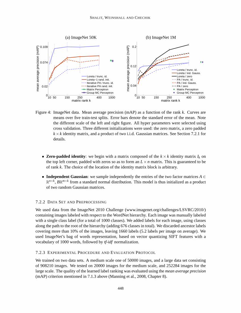
Figure 4: ImageNet data. Mean average precision (mAP) as a function ofthe rankk. Curves aremeans over five train-test splits. Error bars denote the standard error of the mean. Notethe different scale of the left and right figure. All hyper parameters were selected usingcross validation. Three different initializations were used: the zero matrix,a zero paddedk×k identity matrix, and a product of two i.i.d. Gaussian matrices. See Section 7.2.1 fordetails.

• Zero-padded identity: we begin with a matrix composed of thek× k identity matrixIk onthe top left corner, padded with zeros so as to form anL×n matrix. This is guaranteed to beof rankk. The choice of the location of the identity matrix block is arbitrary.

• Independent Gaussian: we sample independently the entries of the two factor matricesA∈R

n×k, BRm×k from a standard normal distribution. This model is thus initialized as a productof two random Gaussian matrices.

7.2.2 DATA SET AND PREPROCESSING

We used data from the ImageNet 2010 Challenge (www.imagenet.org/challenges/LSVRC/2010/)containing images labeled with respect to the WordNet hierarchy. Each imagewas manually labeledwith a single class label (for a total of 1000 classes). We added labels foreach image, using classesalong the path to the root of the hierarchy (adding 676 classes in total). We discarded ancestor labelscovering more than 10% of the images, leaving 1660 labels (5.2 labels per imageon average). Weused ImageNet’s bag of words representation, based on vector quantizing SIFT features with avocabulary of 1000 words, followed bytf-idf normalization.

7.2.3 EXPERIMENTAL PROCEDURE ANDEVALUATION PROTOCOL

We trained on two data sets. A medium scale one of 50000 images, and a large data set consistingof 908210 images. We tested on 20000 images for the medium scale, and 252284 images for thelarge scale. The quality of the learned label ranking was evaluated using themean average precision(mAP) criterion mentioned in 7.1.3 above (Manning et al., 2008, Chapter 8).

448


ImageNet 1M Precision vs. Time(a)

3 4 50

0.1

0.2

rank = 10

mea

n av

erag

e pr

ecis

ion

(mA

P)

LoretaPAMatrix PerceptronGroup MC Perceptron

3 4 50

0.1

0.2

rank = 25

3 4 50

0.1

0.2

rank = 50

3 4 50

0.1

0.2

rank = 150

log10

CPU time (sec)mea

n av

erag

e pr

ecis

ion

(mA

P)

3 4 50

0.1

0.2

rank = 250

log10

CPU time (sec)

3 4 50

0.1

0.2

rank = 400

log10

CPU time (sec)

(b)

3 4 50.1

0.15

0.2

log10

CPU time

mA

P

LoretaPAMatrix PerceptronGroup MC Perceptron

Figure 5: (a) Mean average precision (mAP) as function of single CPU processing time in secondsfor different algorithms and model ranks, presented on a log-scale. Matrix Perceptron(black squares) and Group Multi-Class Perceptron (purple crosses)are both full rank(rank=1000), and their curves are reproduced on all six panels forcomparison. For eachrank and algorithm (LORETA and PA), we used the best performing initialization scheme.(b) mAP of the best performing model for different algorithms and time points.Errorbars represent standard deviation across 5 train-test splits.

449


7.2.4 COMPARISONS

We compared the performance of LORETA on this task with three other approaches:

1. PA - Iterative Passive-Aggressive: same as described in Section 7.1.4 above for the 20Newsgroups experiment.

2. Matrix Perceptron : a full rank stochastic subgradient descent. The model is initialized as azero matrix of size 1660× 1000, and in each round the loss subgradient is subtracted from it.After a sufficient number of rounds, the model is typically full rank and dense.

3. Group Multi-Class Perceptron: a mixed (2,1) norm online mirror descent algorithm (Kakadeet al., 2010). This algorithm encourages a group-sparsity pattern within the learned matrixmodel, thus presenting an alternative form of regularization when compared with low-rankmodels.

LORETA and PA were run using a range of model ranks. For all three methods, thestep size (orthe C parameter for PA) was chosen by 5-fold cross validation on a validation set.

7.2.5 RESULTS

Figure 4 plots the mAP precision of LORETA and PA for different model ranks, while showing onthe right the mAP of the full rank 1000 Matrix Perceptron and(2,1) norm algorithms. LORETA

significantly improves over all other methods across all ranks. However,we note that LORETA,being a non-convex algorithm, does depend significantly on the method of initialization, with thezero-padded identity matrix being the best initialization for lower rank models, and the zero matrixthe best initialization for higher rank models (rank≥ 150).

In Figure 5 we show the accuracy as a function of CPU tim on a single CPU for the differentalgorithms and model ranks. We ran Matlab R2011a on an Intel Xeon 2.27 GHz machine, andused Matlab’s-singlethread flag to control multithreading. The higher-rank LORETA modelsoutperform all others both in the short time scale (∼ 1000 sec.) and the long time scale (∼ 100,000sec.). For some of the higher-rank models there is evident overtraining atsome point, but thisovertraining could be avoided by adopting an early-stopping procedure.

8. Discussion

We presented LORETA, an algorithm which learns a low-rank matrix based on stochastic Rie-mannian gradient descent and efficient retraction to the manifold of low-rank matrices. LORETA

achieves superior precision in a task of learning similarity in high dimensional feature spaces, andin multi-label annotation, where it scales well with the number of classes. A PSDvariant of LORETA

can be used efficiently for low-rank metric learning.There are many ways to tie together different classifiers in a multi-class setting. We have seen

here that a low-rank assumption coupled with a Riemannian SGD procedure outperformed the (2,1)mixed norm. Other approaches leverage the hierarchical structure inherent in many of these tasks.For example, Deng et al. (2011) use the label hierarchy of ImageNet to compute a similarity measurebetween images.

For similarity learning, the approach we take in this paper uses a weak supervision based onranking similar pairs: one only knows that the pair(q,p+) is more similar than the pair(q,p−). In

450


some cases, a stronger supervision signal is available, like the classes ofeach objects are known. Inthese cases, Deng et al. (2011) have shown how to use class identities to construct good features bytraining an SVM classifier on each class and using its scaled output as a feature. They show thatsuch features can lead to very good performance, with the added advantage that the features can belearned in parallel. The weak supervision approach that we take here aimsto handle the case, whichis particularly common in large scale data sets collected through web users’ activity, where weakersupervision is much easier to collect.

In this paper, we used simple sampling schemes for both the similarity learning andmultiple-labelling experiments. More elaborate sampling techniques such as those proposed by Weston et al.(2011), which focus on “hard negatives”, may yield significant performance improvements. Asthese approaches typically involve rank-one gradients when implemented asonline learning algo-rithms, they are well suited for being used in conjunction with LORETA, and this will be the subjectof future work.

LORETA yields a factorized representation of the low-rank matrix. For similarity learning, thesefactors project to a low-dimensional space where similarity is evaluated efficiently. For classifica-tion, it can be viewed as learning two matrix components: one that projects the high dimensionaldata into a low dimension, and a second that learns to classify in the low dimension. In bothapproaches, the low-dimensional space is useful for extracting the relevant structure from the high-dimensional data, and for exploring the relations between large numbers ofclasses.

Acknowledgments

G.C. was supported by the Israeli science foundation Grant 1001/08, and by a Marie Curie rein-tegration grant PIRG06-GA-2009-256566. U.S. and D.W. were supported by the European Unionunder the DIRAC integrated project IST-027787. Uri Shalit is a recipient of the Google EuropeFellowship in Machine Learning, and this research is supported in part bythis Google Fellowship.We would also like to thank the Gatsby Charitable Foundation for its generous support of the ICNC.

Appendix A. Proof of Lemma 2

We formally define the tangent space of a manifold at a point on the manifold, and then describe anauxiliary parametrization of the tangent space to the manifoldM

n,mk at a pointW ∈M n,m

k .

Definition 7 The tangent space TWM to a manifoldM ⊂ Rn at a point W∈M is the linear space

spanned by all the tangent vectors at 0 to smooth curvesγ : R→M such thatγ(0) = W. That is,the set of tangents inRn to smooth curves within the manifold which pass through the point W.

In order to characterize the tangent space ofMn,mk , we look into the properties of smooth curves

γ, where for eacht, γ(t) ∈M n,mk .

For any such curve, because of the rankk assumption, we may assume that for allt ∈ R, thereexist (non-unique) matricesA(t) ∈ R

n×k∗ , B(t) ∈ R

m×k∗ , such thatγ(t) = A(t)B(t)T . We now wish to

find the tangent vectors to these curves. By the product rule we have:

γ(0) = A(0)B(0)T + A(0)B(0)T .

451


SinceW = γ(0) = A(0)B(0)T = ABT we have forW = ABT :

TWMn,mk =

{

AXT +YBT |X ∈ Rm×k,Y ∈ R

n×k}

. (5)

This is because any choice of matricesX, Y such thatX = B, Y = A will give us some tangent vector,and for any tangent vector there exist such matrices. The space aboveis clearly a linear space. Beinga tangent space to a manifold, it has the same dimension as the manifold:(n+m)k−k2.

Recall the definition of the tangent space given in Lemma 1:

TWMn,mk =

{

[

A A⊥]

[

M NT1

N2 0

][

BT

BT⊥

]

: M ∈ Rk×k,N1 ∈ R

(m−k)×k,N2 ∈ R(n−k)×k

}

. (6)

To prove Lemma 2, it is easy to verify by counting that the dimension of the space as definedin Equation (6) above is(n+m)k− k2. Using the notation above, we can see that by takingX =MBT +N1BT

⊥ andY = A⊥N2, the space defined in Equation (6) is included inTWMn,mk as defined in

Equation (5). Since it is a linear subspace of equal dimension, both spaces must be equal�

Appendix B. Proof of Theorem 3

We state the theorem again here.

Theorem 8 Let W∈M n,mk , W = ABT , and W† = B†TA†. Letξ ∈ TWM

n,mk , ξ = ξAB+ξAB⊥+ξA⊥B,

as in 1, and let:

V1 =W+12

ξAB+ξA⊥B−18

ξABW†ξAB−12

ξA⊥BW†ξAB ,

V2 =W+12

ξAB+ξAB⊥−18

ξABW†ξAB−12

ξABW†ξAB⊥ .

The mappingRW(ξ) =V1W

†V2 (7)

is a second order retraction from a neighborhoodΘW ⊂ TWMn,mk toM n,m

k .

Proof To prove that Equation (7) defines a retraction, we first show thatV1W†V2 is a rank-k matrix.Note that there exist matricesZ1 ∈ R

n×k andZ2 ∈ Rm×k such thatV1 = Z1BT and ,V2 = AZT

2 . Asufficient condition for the matricesZ1 andZ2 to be of full rank is that the matrixM is of limitednorm. Thus, for all tangent vectors lying in some neighborhoodΘW ⊂ TWM

n,mk of 0 ∈ TWM

n,mk ,

the above relation is indeed a retraction to the manifold. In practice this is nevera problem, as theset of matrices not of full rank is of zero measure, and in practice we have found these matrices toalways be of full rank. Thus,RW(ξ) =V1W†V2 = Z1BTB(BTB)−1(ATA)−1ATAZT

2 = Z1ZT2 , which,

given thatZ1 andZ2 are of full column rank, is exactly a rank-k, n×mmatrix.Next we show thatRW(ξ) is a retraction, and of second order. It is obvious thatRW(0) = W,

since the projection of the zero vector is zero, and thusξAB, ξAB⊥ andξA⊥B are all zero.ExpandingV1W†V2 up to second order terms inξ, many terms cancel and we end up with:

RW(ξ) =W+ξAB+ξAB⊥+ξA⊥B+ξA⊥BW†ξAB⊥+O(‖ξ‖3)

=W+ξ+ξA⊥BW†ξAB⊥+O(‖ξ‖3).

452


Local first order rigidity is immediately apparent. If we expand the only second order term,ξA⊥BW†ξAB⊥ , we see that it equalsA⊥N2NT

1 BT⊥. We claim this term is orthogonal to the tangent

spaceTWMn,mk . If we take, using the characterization in Lemma 2, an arbitrary tangent vector

AMBT +ANT1 BT⊥+A⊥N2BT in TWM

n,mk , we can calculate the inner product:

⟨(

A⊥N2NT1 BT⊥

)

,(

AMBT +ANT1 BT⊥+A⊥N2BT)⟩=

tr(

B⊥N1NT2 AT⊥AMBT +B⊥N1NT

2 AT⊥ANT

1 BT⊥+B⊥N1NT

2 AT⊥A⊥N2BT)=

tr(

B⊥N1NT2 AT⊥A⊥N2BT)=

tr(

BTB⊥N1NT2 AT⊥A⊥N2

)

= 0

with the equalities stemming from the fact thatAT⊥A= 0, BT

⊥B= 0, and from standard trace identi-ties. Thus, the second order term cancels out if we project the second derivative of the curve definedby the retraction, as required by the second-order condition

PW

(

dRW(τξ)dτ2 |τ=0

)

= 0 ∀ξ ∈ TWM .

We see that the second order term is contained in the normal space. This concludes the proofthat the retraction is a second order retraction.

Appendix C. Proof of Lemma 4

Let us see how can we calculate the needed terms explicitly. When evaluating the expressionV1W†V2, we can use the algebraic relations:WW† = PA andW†W = PB. From this we can concludethat: WW†ξAB = ξAB, ξABW†W = ξAB, ξA⊥BW†W = ξA⊥B andWW†ξAB⊥ = ξAB⊥ . These relations,along with many terms that cancel out, lead to the following expression:

RW(ξ) =V1W†V2 =

W+ξAB+ξAB⊥+ξA⊥B−18

ξABW†ξABW†ξAB−38

ξABW†ξABW†ξAB⊥

−38

ξA⊥BW†ξABW†ξAB+ξA⊥BW†ξAB⊥−ξA⊥BW†ξABW†ξAB⊥

+116

ξABW†ξABW†ξABW†ξAB⊥+116

ξA⊥BW†ξABW†ξABW†ξAB

+164

ξABW†ξABW†ξABW†ξAB+14

ξA⊥BW†ξABW†ξABξAB⊥ .

We now substitute the matricesM, N1 andN2 into the above relation. Most terms cancel out.For example, we have the identityξABW†ξAB = AM2BT , ξABW†ξABW†ξAB = AM3BT and so forth.We obtain the following relation:

RW(ξ) = ABT +AMBT +ANT1 BT⊥+A⊥N2BT −

18

AM3BT

−38

AM2NT1 BT⊥−

38

A⊥N2M2BT +A⊥N2NT1 BT⊥−A⊥N2MNT

1 BT⊥

+116

AM3NT1 BT⊥+

116

A⊥N2M3BT +164

AM4BT +14

A⊥N2M2NT1 BT⊥.

453


Collecting terms by the leftmost and rightmost factors, we obtain:

RW(ξ) = A

(

Ik+M−18

M3+164

M4)

BT

+A

(

Ik−38

M2+116

M3)

NT1 BT⊥

+A⊥N2

(

Ik−38

M2+116

M3)

BT

+A⊥N2

(

Ik−M+14

M2)

NT1 BT⊥ .

Finally, treating the first and fourth lines as a polynomial expression inM, and taking its poly-nomial square root, we can split the above sum into the product of ann× k matrix and ak×mmatrix:

RW(ξ) =[

A

(

Ik+12

M−18

M2)

+A⊥N2

(

Ik−12

M

)]

·

[

B

(

Ik+12

MT −18

(

MT)2)

+B⊥N1

(

Ik−12

MT)]T

.

Appendix D. Rank One Pseudoinverse Update Rule

For completeness we develop below the procedure for updating the pseudoinverse of a rank-1 per-turbed matrix (Meyer, 1973), following the derivation of Petersen and Pedersen (2008). We wishto find a matrixG such that for a given matrixA along with its pseudo-inverseA†, and vectors ofappropriate dimensionc andd, we have:

(

A+cdT)†= A†+G.

We have used the fact thatA has a full column rank to simplify slightly the algorithm of Petersenand Pedersen (2008).

References

P.-A. Absil and J. Malick. Projection-like retractions on matrix manifolds. Technical Report UCL-INMA-2010.038, Department of Mathematical Engineering, Université catholique de Louvain,July 2010.

P.-A. Absil, R. Mahony, and R. Sepulchre.Optimization Algorithms on Matrix Manifolds. PrincetonUniv Press, 2008.

B. Bai, J. Weston, R. Collobert, and D. Grangier. Supervised semantic indexing. Advances inInformation Retrieval, pages 761–765, 2009.

A. Bar-Hillel, T. Hertz, N. Shental, and D. Weinshall. Learning a mahalanobis metric from equiva-lence constraints.Journal of Machine Learning Research, 6(1):937–965, 2006.

454


Algorithm 7 : Rank one pseudo-inverse update

Input: MatricesA,A† ∈ Rn×k∗ , such thatA† is the pseudo-inverse ofA, vectorsc∈ R

n×1, d ∈ Rk×1

Output: Matrix Z† ∈ Rk×n∗ , such thatZ† is the pseudo-inverse ofA+cdT .

Compute: matrix dimensionv= A†c k×1β = 1+dTv 1×1n= A†Td n×1n= A†n k×1w= c−Av n×1if β 6= 0 AND ‖w‖ 6= 0

G= 1β nwT k×n

s= β‖w‖2‖n‖2+β2 1×1

t = ‖w‖2

β n+v k×1

G= s· t(

‖n‖2

β w+n)T

k×n

G= G− G k×nelseifβ = 0 AND ‖w‖ 6= 0

G=−A† n‖n‖2 k×1

G= GnT k×1G= v wT

‖w‖2 k×n

G= G− G k×nelseifβ 6= 0 AND ‖w‖= 0

G=− 1βvnT k×n

elseifβ = 0 AND ‖w‖= 0v= 1

‖v‖2 v(

vTA†)

k×n

n= 1‖n‖2

(

A†n)

nT k×n

G= vTA†n‖v‖2‖n‖2 vnT − v− n k×n

endifZ† = A†+G

J. Briët, F.M. de Oliveira Filho, and F. Vallentin. The Grothendieck problemwith rank constraint.In Proceedings of the 19th International Symposium on Mathematical Theory of Networks andSystems, MTNS, 2010.

G. Chechik, V. Sharma, U. Shalit, and S. Bengio. Large scale online learning of image similaritythrough ranking.Journal of Machine Learning Research, 11:1109–1135, 2010.

K. Crammer, O. Dekel, J. Keshet, S. Shalev-Shwartz, and Y. Singer. Online passive-aggressivealgorithms.Journal of Machine Learning Research, 7:551–585, 2006.

J. Deng, W. Dong, R. Socher, L.J. Li, K. Li, and L. Fei-Fei. Imagenet: Alarge-scale hierarchicalimage database. InProceedings of the 22nd IEEE Conference on Computer Vision and Pattern

455


Recognition, pages 248–255, 2009.

J. Deng, A. Berg, and L. Fei-Fei. Hierarchical Semantic Indexing for Large Scale Image Retrieval.In Proceedings of the 24th IEEE Conference on Computer Vision and PatternRecognition, pages785–792, 2011.

M.P. Do Carmo.Riemannian Geometry. Birkhauser, 1992.

L. Eldén and B. Savas. A Newton–Grassmann method for computing the bestmulti-linear rank-(r1,r2, r3) approximation of a tensor.SIAM Journal on Matrix Analysis and applications, 31(2):248–271, 2009.

M. Fazel.Matrix Rank Minimization with Applications. PhD thesis, Electrical Engineering Depart-ment, Stanford University, 2002.

M. Fazel, H. Hindi, and S. Boyd. Rank minimization and applications in system theory. In Pro-ceedings of the 2004 American Control Conference, pages 3273–3278. IEEE, 2005.

A. Globerson and S. Roweis. Metric learning by collapsing classes. InAdvances in Neural Infor-mation Processing Systems, volume 18, page 451, 2006.

J. Goldberger, S. Roweis, G. Hinton, and R. Salakhutdinov. Neighbourhood components analysis.In Advances in Neural Information Processing Systems, volume 17, 2005.

D. Grangier and S. Bengio. A discriminative kernel-based model to rank images from text queries.IEEE Transactions on Pattern Analysis and Machine Intelligence, 30:1371–1384, 2008.

M. Ishteva, L. De Lathauwer, P.-A. Absil, and S. Van Huffel. Best low multilinear rank approxi-mation of higher-order tensors, based on the Riemannian trust-region scheme.SIAM Journal onMatrix Analysis and Applications, 32(1):115–132, 2011.

P. Jain, B. Kulis, I.S. Dhillon, and K. Grauman. Online metric learning and fast similarity search.In Advances in Neural Information Processing Systems, volume 20, pages 761–768, 2008.

P. Jain, R. Meka, and I. Dhillon. Guaranteed rank minimization via singular value projection. InAdvances in Neural Information Processing Systems, volume 24, pages 937–945, 2011.

M. Journée, F. Bach, P.-A. Absil, and R. Sepulchre. Low-Rank Optimization on the Cone of PositiveSemidefinite Matrices.SIAM Journal on Optimization, 20(5):2327–2351, 2010a.

M. Journée, Y. Nesterov, P. Richtárik, and R. Sepulchre. Generalized power method for sparseprincipal component analysis.The Journal of Machine Learning Research, 11:517–553, 2010b.

S.M. Kakade, S. Shalev-Shwartz, and A. Tewari. Regularization techniques for learning with ma-trices, 2010. Arxiv preprint arXiv:0910.0610v2.

R.H. Keshavan, A. Montanari, and S. Oh. Matrix completion from noisy entries. The Journal ofMachine Learning Research, 99:2057–2078, 2010.

B. Kulis, M.A. Sustik, and I.S. Dhillon. Low-rank kernel learning with bregman matrix divergences.The Journal of Machine Learning Research, 10:341–376, 2009.

456


K. Lang. Learning to filter netnews. InProceeding of the 12th Internation Conference on MachineLearning, pages 331–339, 1995.

C.D. Manning, P. Raghavan, H. Schutze, and Ebooks Corporation.Introduction to InformationRetrieval, volume 1. Cambridge University Press Cambridge, UK, 2008.

R. Meka, P. Jain, C. Caramanis, and I.S. Dhillon. Rank minimization via online learning. InProceedings of the 25th International Conference on Machine learning, pages 656–663, 2008.

C.D. Meyer. Generalized inversion of modified matrices.SIAM Journal on Applied Mathematics,24(3):315–323, 1973.

G. Meyer, S. Bonnabel, and R. Sepulchre. Regression on fixed-rank positive semidefinite matrices:a Riemannian approach.The Journal of Machine Learning Research, 12:593–625, 2011.

B.K. Natarajan. Sparse approximate solutions to linear systems.SIAM Journal on Computing, 24(2):227–234, 1995.

Sahand Negahban and Martin J. Wainwright. Estimation of (near) low-rankmatrices with noiseand high-dimensional scaling. InProceedings of the 27th International Conference on MachineLearning, pages 823–830, 2010.

C. Oberlin and S.J. Wright. Active set identification in nonlinear programming.SIAM Journal onOptimization, 17(2):577–605, 2007.

K.B. Petersen and M.S. Pedersen. The matrix cookbook, Oct. 2008.

B. Recht, M. Fazel, and P.A. Parrilo. Guaranteed minimum-rank solutions of linear matrix equationsvia nuclear norm minimization.SIAM Review, 52(3):471–501, 2010.

S. Shalev-Shwartz, Y. Singer, and A.Y. Ng. Online and batch learning ofpseudo-metrics. InProceedings of the Twenty-first International Conference on MachineLearning, page 94. ACM,2004.

Uri Shalit, Daphna Weinshall, and Gal Chechik. Online learning in the manifoldof low-rank ma-trices. InAdvances in Neural Information Processing Systems 23, pages 2128–2136. MIT Press,2010.

B. Vandereycken and S. Vandewalle. A Riemannian optimization approach for computing low-ranksolutions of Lyapunov equations.SIAM Journal on Matrix Analysis and Applications, 31(5):2553–2579, 2010.

B. Vandereycken, P.-A. Absil, and S. Vandewalle. Embedded geometry of the set of symmetricpositive semidefinite matrices of fixed rank. InStatistical Signal Processing, 2009. SSP’09.IEEE/SP 15th Workshop on, pages 389–392. IEEE, 2009.

K.Q. Weinberger and L.K. Saul. Distance metric learning for large margin nearest neighbor classi-fication. The Journal of Machine Learning Research, 10:207–244, 2009.

457


J. Weston, S. Bengio, and N. Usunier. Wsabie: Scaling up to large vocabulary image annotation.In Proceedings of the 22nd International Joint Conference on Artificial Intelligence (IJCAI–11),2011.

E.P. Xing, A.Y. Ng, M.I. Jordan, and S. Russell. Distance metric learning, with application to clus-tering with side-information. InAdvances in Neural Information Processing Systems, volume 15,pages 505–512. MIT Press, 2002.

L. Yang. An overview of distance metric learning. Technical report, School of Computer Science,Carnegie Mellon University, 2007.

Y. Yang and J.O. Pedersen. A comparative study on feature selection in text categorization. InProceedings of the 14th International Conference on Machine Learning, pages 412–420, 1997.

458

Documents

Online Learning in the Embedded Manifold of Low-rank Matrices