Luenberger Indicator and Directions of Measurement: A

Luenberger Indicator and Directions of Measurement: A Bottoms-up

Approach with an Empirical Illustration to German Saving Banks

Mohsen Afsharian1 and Heinz Ahn

Department of Business Sciences, Technische Universität Braunschweig, Fallersleber-Tor-Wall 23, 38100

Braunschweig, Germany

1 Corresponding author. Email: [email protected]; Phone: +495313913606; Fax: +495313918121

https://doi.org/10.24355/dbbs.084-201902080916-0

mailto:[email protected]

1 Luenberger Indicator and Directions of Measurement: A Bottoms-up Approach with an Empirical Illustration to German Saving Banks

Luenberger Indicator and Directions of Measurement: A Bottoms-up

Approach with an Empirical Illustration to German Saving Banks

Abstract. The Luenberger productivity indicator applies directional distance functions which allow

to specifying in what direction (i.e. direction of measurement) the operating units will be evaluated.

In the presence of a change in the direction of measurement, the standard components of the

existing Luenberger productivity indicator may provide values which are not compatible with

reality. In order to eliminate this pitfall, the so-called bottoms-up approach is used to revisit the

definition of the indicator and its components. We start with a list of selected sources of

productivity change, namely efficiency change, technical change and direction change, then

examine the best possible way of measuring each of the sources and combine them to derive a new

measure of productivity change. The proposed indicator will be illustrated by means of an empirical

application to a panel of 417 German saving banks over the time period 2006-2012. The example

explains how the proposed approach is able to properly measure efficiency change, technical

change and direction change. The results also provide conclusive evidence about the effect of the

change in direction of measurement on the results of the productivity over time in a centralized

management scenario.

Keywords: Data Envelopment Analysis (DEA); productivity measurement; direction change;

banking

JEL Classification C44, C67, D24



1. Introduction

Among the different indices for measuring productivity changes of decision making units (DMUs)

over time, Malmquist indices have commonly been used by researchers and practitioners in various

environments. Examples include the health sector (e.g., see Kirigia et al. 2007; Chowdhury et al.

2011), the electricity industry (e.g., see Tovar et al. 2011; Aghdam 2011), telecommunications (e.g.,

see Lam and Shiu 2010; Hisali and Yawe 2011), the water industry (e.g., see Corton and Berg 2009;

Portela et al. 2011), agriculture (e.g., see Kao 2010; Xu 2012), transportation (e.g., see Gitto and

Mancuso 2012; Pires and Fernandes 2012), the banking industry (e.g., see Asmild et al. 2004;

Portela and Thanassoulis 2010) and others.

Caves et al. (1982) introduced the earliest type of the Malmquist index and showed how the change

in productivity experienced by an operating unit can be measured over time. Nischimizu and Page

(1982) identified technological change and change in technical efficiency as two components of

productivity change over time. Färe et al. (1992) used data envelopment analysis (DEA), proposed

by Farrell (1957) and developed by Charnes et al. (1978), as mathematical programming-based

methodology to measure the Malmquist productivity index. In the same paper, they also showed

how the Malmquist index can be exhibited as the product of technical change and efficiency change

components (i.e. FGLR decomposition of the Malmquist index). After this seminal work, there have

been a considerable number of studies in the literature about the framework (see, e.g. Berg et al.

1992; Shestalova 2003; Pastor and Lovell 2005; Pastor et al. 2011), decomposition (see, e.g., Färe

et al. 1994; Ray and Desli 1997; Wheelock and Wilson 1999; Gilbert and Wilson 1998; Grifell-

Tatje and Lovell 1999), and computation (see, e.g., Chen 2003; Grifell-Tatje et al. 1998; Portela et

al. 2004) of the Malmquist index.

Since the introduction of the primal Malmquist index by Färe et al. (1992), one of the limitations

often faced by researchers in measuring this index has been to choose either an input- or an output-

oriented perspective. The reason is that the Malmquist index requires a choice to be made between

an input distance function and an output distance function yielding the input and output Malmquist

productivity indices, respectively. In contrast, many practical situations suggest to combine both

views, i.e. input-saving and output-expanding scenarios have to be taken into account

simultaneously. In order to overcome this limitation, Chambers et al. (1996) introduced the

Luenberger productivity indicator (hereafter named Luenberger indicator) for measuring

productivity changes over time. The authors showed that this indicator, which has an additive

structure rather than multiplicative, contains the input/output Malmquist productivity indices as its

special cases. Motivated by FGLR decomposition of the Malmquist index, they also describe how



the Luenberger indicator can be decomposed into technical change (shift in the frontier of the

benchmark technology) and changes in technical efficiency (change in the individual initiatives and

activities) as two components of productivity change over time.

The Luenberger indicator applies directional distance functions which allow to specifying in what

direction (i.e. direction of measurement) the operating units will be evaluated (see, e.g., Färe and

Grosskopf 2000). Within this framework, the performance of a unit is characterized by measuring

the distance to the boundary of the benchmark technology along the predetermined direction of

measurement, i.e. a directed distance is defined. This property provides the possibility to work with

a multidirectional productivity analysis in a way that a desired structure (e.g., central management’s

preference) concerning the potential improvement of inputs and outputs can be incorporated. It also

enables to deal with special structures of input/output data when measuring productivity changes

over time. Examples are the Luenberger-type indicators to measure environmentally sensitive

productivity growth where some outputs are undesirable (see, e.g., Chung et al. 1997) and to

measure productivity change under negative data (see, e.g., Portela et al. 2010). Among other

advantages (see, e.g., Chambers et al. 1998), the above-described property of directional distance

functions has made the Luenberger indicator an important managerial tool which can facilitate

decision making and control in performance management systems.

A review of the studies focusing on multiple time period analysis leads to the conclusion that not

only the shape and the characteristics of the benchmark technology can change (e.g., due to policy

directives, the competitive situation and economic conditions) but also the direction of

measurement. Among different situations in which the direction of measurement is likely to change

over time, we address the scenario that a centralized management exists which supervises the

operating units. In such cases, the centralized management of the organization is often responsible,

e.g., for coordinating decision making within the group, determining strategic directions and

making general policy decisions as well as monitoring the activities of the operating units. Within

this scenario, some variables are controlled by the central management not only to promote

efficiency and effectiveness but also to improve the level of learning, coordination and motivation

among the operating units (Bogetoft and Otto 2011). Possible examples concern organizations with

operating units like bank branches, pharmacy stores, university departments, police stations etc.

(different perspectives on centralized assessment of operating units by DEA can be found, e.g., in

Athanassopoulos 1995; Li and Ng 1995; Lozano and Villa 2004; Cook and Zhu 2007; Asmild et al.

2009; Ahn et al. 2012; Fang 2013).



In cases like that, a preferred direction of measurement can be determined with regard to the

corporate strategy and overall goals of the organization. This direction is usually beyond the control

of local managers and may change over time. Thereby, the responsible employees in the operating

units are often rewarded on the basis of the results from the performance measurement system (for a

detailed discussion of this issue see, e.g., Langfield-Smith 1997; Nudurupati et al. 2011). In such a

context, any change in the direction of measurement can force the operating units to adapt their

local variables (e.g., local strategy, scale of operation etc.) in order to avoid their productivity to be

affected over time. Accordingly, apart from efficiency change (change in the individual initiatives

and activities) and technical change (shift in the frontier of the benchmark technology) as two

standard drivers of productivity change, any regress or progress in the productivity of a unit may

also be explained by considering the change in the direction of measurement.

As it will be shown, the existing two-way decomposition of the Luenberger indicator is unable to

distinguish between the shift in the frontier of the benchmark technology and the change in the

direction of measurement. Consequently, in the presence of a change in the direction of

measurement, the standard components of the Luenberger indicator may provide values which are

not compatible with reality. This pitfall has not been identified or solved so far in previous studies

where the direction of measurement is addressed and, among others, is defined as the mean values

(see, e.g., Park and Weber 2006) or the ideal point (see, e.g., Portela and Thanassoulis 2010) of the

data in each time period. Against this background, we revisit the Luenberger indicator and its

components in order to remedy the outlined pitfall. Using the bottoms-up approach suggested by

Balk (2001) we start with a list of selected sources of productivity change, examine the best

possible way of measuring each of these sources and combine them to derive a new measure of

productivity change. The new indicator will not only properly measure efficiency change and

technical change components, but is also able to capture the degree to which predetermined

directions of measurement affect the productivity of units over time.

The paper proceeds as follows: Section 2 presents an overview of the process of efficiency

measurement by means of directional distance functions. It will also be shown how performance,

which comprises magnitude and direction, can systematically be affected by different specifications

of both benchmark technology and direction of measurement. In section 3, it will be investigated

why the existing two-way decomposition of the Luenberger indicator is unable to properly measure

productivity change in the presence of a change in the direction of measurement. The proposed

Luenberger indicator and the corresponding components – namely efficiency change, technical

change and direction change – will be introduced and described in Section 4. The mathematical

aspects of the proposed indicator will also be investigated. Section 5 analyzes the proposed



Luenberger indicator and its advantages on the basis of an empirical illustration to a panel of 417

German saving banks over the time period 2006-2012. Section 6 concludes the paper with a

summary and an outlook on future research opportunities.

2. Benchmark technology and directional distance function

Suppose that there exist n DMUs in t (t = 1,…,T) time periods. Let 1 2( )t t t t mj j j mjX x ,x ,...,x += ∈ℜ and

1 2( )t t t t sj j j sjY y , y ,..., y += ∈ℜ be non-zero vectors which quantify the level of inputs and outputs of

DMUj in period t. The benchmark technology, which is defined as the set of all feasible

combinations of input and output quantities in t, is usually shown as:

{ }( ) can produce .t t t m s t tT X ,Y X Y+ += ∈ℜ ×ℜ (1)

In terms of properties satisfied by each benchmark technology, tT can be characterized precisely by

applying desired mathematical axioms such as free disposability, returns to scale, convexity etc.

(see, e.g., Charnes et al. 1978; Banker et al. 1984). Throughout the paper, without loss of generality

(see, e.g., Färe et al. 1994), we assume that each benchmark technology satisfies the following

axioms:

1. (Non-emptiness). The observed ( , )t t tj jX Y T∈ , j = 1,…,n.

2. (Free disposability). If ( , ) , ,tX Y T X X Y Y′ ′∈ ≥ ≤ , then ( , ) tX Y T′ ′ ∈ .

3. (Constant returns to scale). If ( , ) tX Y T∈ , then ( , ) tX Y Tα α ∈ for all 0α ≥ .

4. (Convexity). If ( , )X Y and ( , )X Y% %, then ( , ) (1 )( , ) tX Y X Y Tλ λ+ − ∈% % for any [ ]0 1,λ∈ .

5. (Minimum extrapolation). tT is the smallest set which satisfies axioms 1 to 4.

The benchmark technology in time period t can now be specified as follows:

1 1( ) ; 0; 1 .

n nt t t m s t t t t t t t

j ij j rj jj j

T X ,Y X λ x , Y λ y λ j ,...,n+ += =

= ∈ℜ ×ℜ ≥ ≤ ≥ =

∑ ∑ (2)

Following Chambers et al. (1998), the directional distance function which simultaneously seeks to

expand the outputs and contract the inputs in time period t can be defined as:



{ }( , , ) sup :( , ) ( , ) ,t t t t t tx y x yD X ,Y d d X Y d d Td d= + − ∈% (3)

where ( , )x yd d d= −ur

defines a directional vector so that 1 2( ) += ∈ℜmx x x xmd d ,d ,...,d and

1 2( ) += ∈ℜsy y y ysd d ,d ,...,d . This direction allows us to work with a multidirectional efficiency

analysis by which we can incorporate a desired structure (e.g., central management’s preference)

over the potential improvement of inputs and outputs. Detailed properties of the directional distance

function can be found in Chambers et al. (1996; 1998).

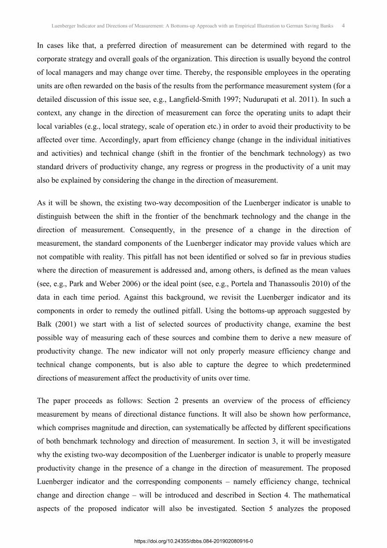
Figure 1 illustrates the process of measurement by means of a simple case of production process in

which a single input is used to produce a single output.

Figure 1. Benchmark technology and directional distance function.

According to definition (3), given a directional vector dur

, ( , )t tX Y is projected onto the boundary

of the technology tT at * *( , )t tx yX d Y dd d− + , where * ( , , )t t t

x yD X ,Y d dd = % . On this basis, the

value of the distance function *d depends not only on the characteristics of the benchmark

technology tT , but also on the direction of measurement dur

as well as on the corresponding

distance of the unit under evaluation from the frontier of the benchmark technology. In other words,

the performance comprises both magnitude and direction and is systematically affected by different

specifications of both the benchmark technology and the direction of measurement. Therefore, this

can be considered as a primary motivation to distinguish between properties which characterize the

benchmark technology and the choice of direction by which the performance is measured. The

reason is that, on one hand, the performance is concerned by the shape of the benchmark technology

which can be affected itself by regulations, competitive situations and economic conditions etc. On

the other hand, it can be significantly oriented towards the direction of measurement determined

with regard to the corporate strategy and overall goals of the organization. A detailed discussion of



the role of the benchmark technology in the process of efficiency measurement can be found, e.g.,

in Grosskopf (1986).

3. The Luenberger indicator and change in the direction of measurement

Suppose that an individual unit, DMUp (p = 1,…,n), in time periods t and t+1 is represented by

( )t t tp p pDMU X ,Y= and 1 1 1( )t t t

p p pDMU X ,Y+ + += , respectively. In order to measure the productivity

change for this unit between the two time periods, the directional distance functions can be

determined corresponding to either the first technology tT or the second technology 1tT + as best-

practice reference. Accordingly, Chambers et al. (1996) define the Luenberger indicator, here

denoted by 1 1( , )t t t tp p p pLI X ,Y X ,Y+ + , as the arithmetic mean of the two measures of productivity

change which are computed on the benchmark technologies t and t+1 as follows:

{

1 1

1 1 1 1

1 1

( , )1 ( , , ) ( , , )2

( , , ) ( , , )

t t t tp p p p

t t t t t tp p x y p p x y


LI X ,Y X ,Y

D X ,Y d d D X ,Y d d


+ +

+ + + +

+ +

= − +

−

% %

% %

(4)

Furthermore, it has been shown that the Luenberger indicator can additively be decomposed into the

following components (for further details see, e.g., Chambers et al. 1996):

1 1 1

1 1 1

( ) ( , , ) ( , , )

( , , ) ( , , )



Efficiency Change EC TE X ,Y d d TE X ,Y d d


+ + +

+ + +

= −

= −% % (5)

{}

1, 1 1

1 1 1 1 1

1

( ) ( , , , )1 ( , , ) ( , , )2

( , , ) ( , , )

t t t t t tp p p p x y



Technical Change TC TC X ,Y X ,Y d d



+ + +

+ + + + +

+

=

= −

+ −

% %

% %

(6)

This decomposition reveals that the change in productivity can be affected by two components. The

former is efficiency change (EC). It captures the change in the technical efficiency of the unit under

consideration between time periods t and t+1. The latter is technical change (TC). It is computed by

an arithmetic mean of the two basic technical changes which represent the change in the frontier of

the benchmark technology between the two time periods.

If the value of the Luenberger indicator or any of its components is less than one, it denotes regress,

while a value greater than one implies progress; a value of one indicates an unchanged situation. In



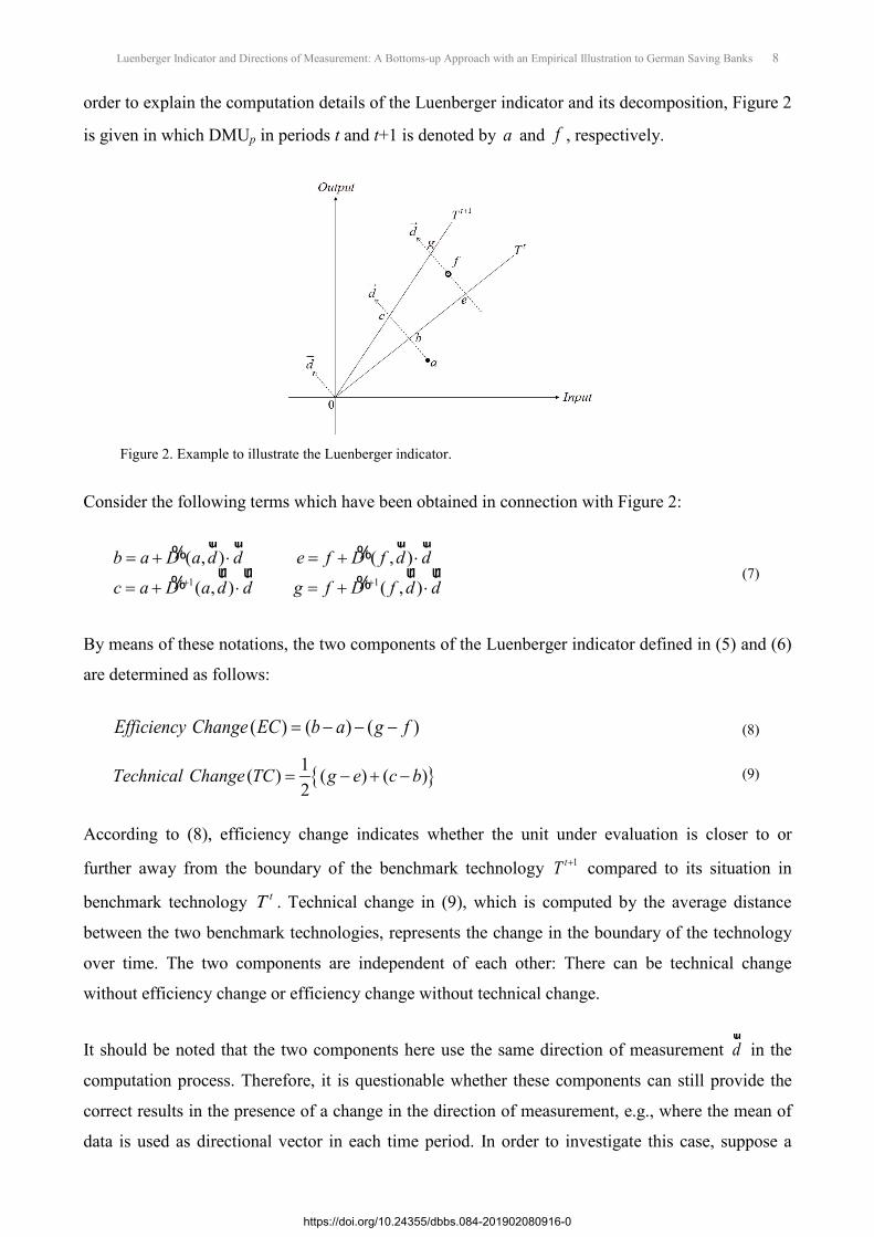
order to explain the computation details of the Luenberger indicator and its decomposition, Figure 2

is given in which DMUp in periods t and t+1 is denoted by a and f , respectively.

Figure 2. Example to illustrate the Luenberger indicator.

Consider the following terms which have been obtained in connection with Figure 2:

1 1

( , ) ( , )

( , ) ( , )

t t

t t

b a D a d d e f D f d d

c a D a d d g f D f d d+ +

= + ⋅ = + ⋅

= + ⋅ = + ⋅

ur ur ur ur% %ur ur ur ur% %

(7)

By means of these notations, the two components of the Luenberger indicator defined in (5) and (6)

are determined as follows:

( ) ( ) ( )Efficiency Change EC b a g f= − − − (8)

{ }1( ) ( ) ( )2

Technical Change TC g e c b= − + − (9)

According to (8), efficiency change indicates whether the unit under evaluation is closer to or

further away from the boundary of the benchmark technology 1tT + compared to its situation in

benchmark technology tT . Technical change in (9), which is computed by the average distance

between the two benchmark technologies, represents the change in the boundary of the technology

over time. The two components are independent of each other: There can be technical change

without efficiency change or efficiency change without technical change.

It should be noted that the two components here use the same direction of measurement dur

in the

computation process. Therefore, it is questionable whether these components can still provide the

correct results in the presence of a change in the direction of measurement, e.g., where the mean of

data is used as directional vector in each time period. In order to investigate this case, suppose a



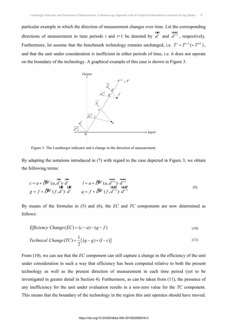
particular example in which the direction of measurement changes over time. Let the corresponding

directions of measurement in time periods t and t+1 be denoted by tduur

and 1td +uuur

, respectively.

Furthermore, let assume that the benchmark technology remains unchanged, i.e. 1 ( )t t UCT T T+= = ,

and that the unit under consideration is inefficient in either periods of time, i.e. it does not operate

on the boundary of the technology. A graphical example of this case is shown in Figure 3.

Figure 3. The Luenberger indicator and a change in the direction of measurement.

By adapting the notations introduced in (7) with regard to the case depicted in Figure 3, we obtain

the following terms:

1 1

1 1

( , ) ( , )

( , ) ( , )

UC t t UC t t

UC t t UC t t

c a D a d d l a D a d d

g f D f d d q f D f d d

+ +

+ +

= + ⋅ = + ⋅

= + ⋅ = + ⋅

uur uur uuur uuur% %


(9)

By means of the formulas in (5) and (6), the EC and TC components are now determined as

follows:

( ) ( ) ( )Efficiency Change EC c a q f= − − − (10)

{ }1( ) ( ) ( )2

Technical Change TC q g l c= − + − (11)

From (10), we can see that the EC component can still capture a change in the efficiency of the unit

under consideration in such a way that efficiency has been computed relative to both the present

technology as well as the present direction of measurement in each time period (yet to be

investigated in greater detail in Section 4). Furthermore, as can be taken from (11), the presence of

any inefficiency for the unit under evaluation results in a non-zero value for the TC component.

This means that the boundary of the technology in the region this unit operates should have moved.



However, this is obviously not the case, what can be observed from the figure which is based on the

primal assumption that 1 ( )t t UCT T T+= = . It must therefore be concluded that the current TC

component is unable to properly characterize technological progress/regress as change in the

boundary of the technology. The reason is that this component does not distinguish between the

change in frontier technology and another important factor which can capture the change in the

direction of measurement. In the presence of such a kind of change, the TC component and

accordingly the entire decomposition may provide values which are not compatible with what has

been experienced in reality.

In order to eliminate the depicted pitfall, the so-called bottoms-up approach is used in the following

to revisit the definition of the aforementioned components in the presence of change in the direction

of measurement. More precisely, we start with a list of selected sources of productivity change, then

examine the best possible way of measuring each of the sources and combine them to derive a

measure of productivity change. As it will be shown, the resulting new indicator properly measures

efficiency change as well as technical change components and is able to capture the degree to which

predetermined directions of measurement affect the productivity of units over time.

4. The proposed Luenberger indicator

4.1 Notations

Consider n DMUs observed in time period t (t = 1,…,T). We use the same notations for the level of

inputs and outputs as well as the same assumptions for the benchmark technologies as introduced in

Section 2. We consider the case that not only the benchmark technology can change over time but

also the direction of measurement. Therefore, we use the following modified notation of the

directional distance function:

{ }( ) sup :( , ) ( , ) ,t

tT t t t t t t t

x ydD X ,Y X Y d d Td d= + − ∈% (12)

where ( , )t t tx yd d d= −

uur defines a directional vector in time period t (t = 1,…,T) so that

1 2( ) += ∈ℜt t t t mx x x xmd d ,d ,...,d and 1 2( ) += ∈ℜt t t t s

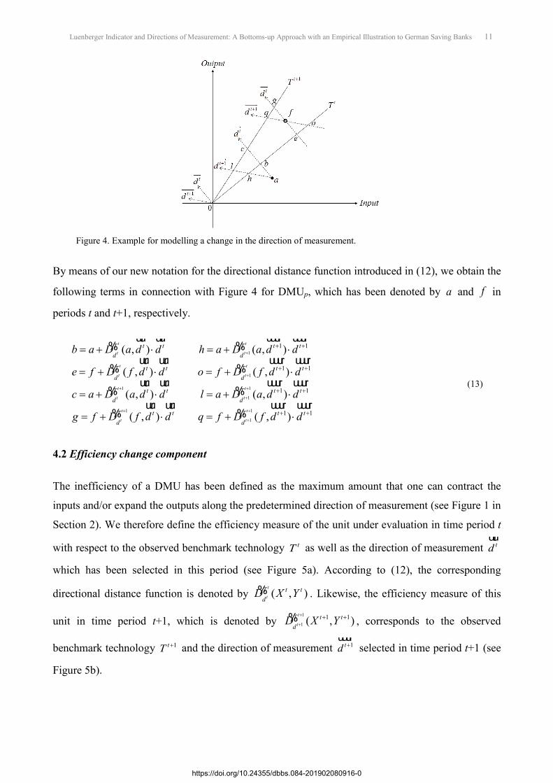
y y y ysd d ,d ,...,d . Figure 4 shows a graphical example

with two time periods t and t+1, accordingly two benchmark technologies tT and 1tT + as well as

two directions of measurement tduur

and 1td +uuur

.



Figure 4. Example for modelling a change in the direction of measurement.

By means of our new notation for the directional distance function introduced in (12), we obtain the

following terms in connection with Figure 4 for DMUp, which has been denoted by a and f in

periods t and t+1, respectively.

1

1

1 1

1

1

1 1

1 1

1 1

( , ) ( , )

( , ) ( , )

( , ) ( , )

( , )

t t

t t

t t

t t

t t

t t

t

t

T t t T t td d

T t t T t td d

T t t T t td d

T td

b a D a d d h a D a d d

e f D f d d o f D f d d

c a D a d d l a D a d d

g f D f d

+

+

+ +

+

+

+ +

+ +

+ +

= + ⋅ = + ⋅

= + ⋅ = + ⋅

= + ⋅ = + ⋅

= + ⋅




uur% 1

11 1( , )

t

tt T t t

dd q f D f d d

+

++ += + ⋅

uur uuur uuur%

(13)

4.2 Efficiency change component

The inefficiency of a DMU has been defined as the maximum amount that one can contract the

inputs and/or expand the outputs along the predetermined direction of measurement (see Figure 1 in

Section 2). We therefore define the efficiency measure of the unit under evaluation in time period t

with respect to the observed benchmark technology tT as well as the direction of measurement tduur

which has been selected in this period (see Figure 5a). According to (12), the corresponding

directional distance function is denoted by ( , )t

tT t td

D X Y% . Likewise, the efficiency measure of this

unit in time period t+1, which is denoted by 1

11 1( , )

t

tT t td

D X Y+

++ +% , corresponds to the observed

benchmark technology 1tT + and the direction of measurement 1td +uuur

selected in time period t+1 (see

Figure 5b).



(a)

(b)

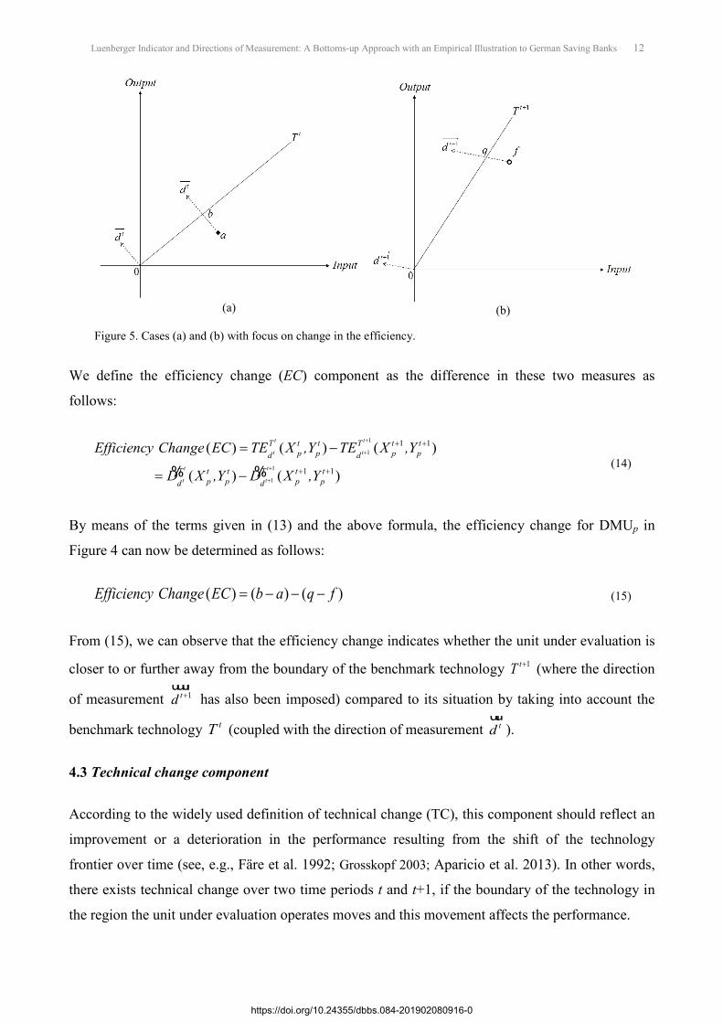
Figure 5. Cases (a) and (b) with focus on change in the efficiency.

We define the efficiency change (EC) component as the difference in these two measures as

follows:

1

1

1

1

1 1

1 1

( ) ( ) ( )

( ) ( )

t t

t t

t t

t t

T t t T t tp p p pd d

T t t T t tp p p pd d

Efficiency Change EC TE X ,Y TE X ,Y

D X ,Y D X ,Y

+

+

+

+

+ +

+ +

= −

= −% % (14)

By means of the terms given in (13) and the above formula, the efficiency change for DMUp in

Figure 4 can now be determined as follows:

( ) ( ) ( )Efficiency Change EC b a q f= − − − (15)

From (15), we can observe that the efficiency change indicates whether the unit under evaluation is

closer to or further away from the boundary of the benchmark technology 1tT + (where the direction

of measurement 1td +uuur

has also been imposed) compared to its situation by taking into account the

benchmark technology tT (coupled with the direction of measurement tduur

).

4.3 Technical change component

According to the widely used definition of technical change (TC), this component should reflect an

improvement or a deterioration in the performance resulting from the shift of the technology

frontier over time (see, e.g., Färe et al. 1992; Grosskopf 2003; Aparicio et al. 2013). In other words,

there exists technical change over two time periods t and t+1, if the boundary of the technology in

the region the unit under evaluation operates moves and this movement affects the performance.



(a)

(b)

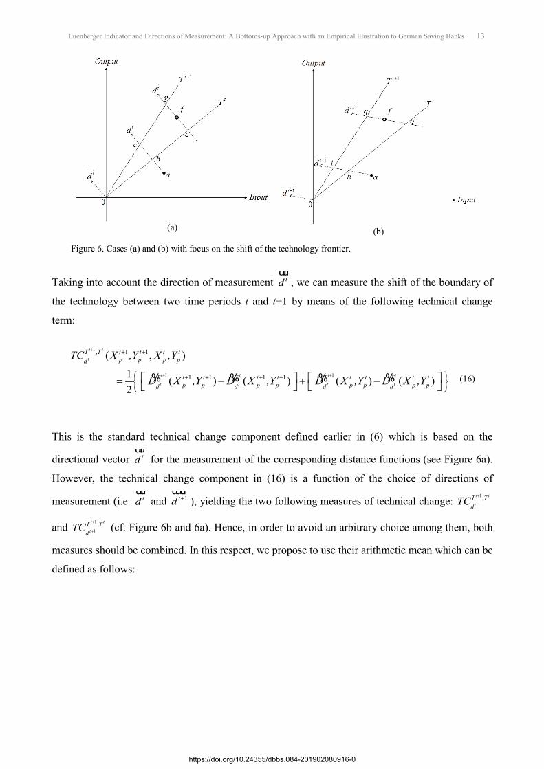
Figure 6. Cases (a) and (b) with focus on the shift of the technology frontier.

Taking into account the direction of measurement tduur

, we can measure the shift of the boundary of

the technology between two time periods t and t+1 by means of the following technical change

term:

{ }

1

1 1

, 1 1

1 1 1 1

( , )

1 ( ) ( ) ( ) ( )2

t t

t

t t t t

t t t t

T T t t t tp p p pd

T t t T t t T t t T t tp p p p p p p pd d d d

TC X ,Y X ,Y

D X ,Y D X ,Y D X ,Y D X ,Y

+

+ +

+ +

+ + + + = − + − % % % %

(16)

This is the standard technical change component defined earlier in (6) which is based on the

directional vector tduur

for the measurement of the corresponding distance functions (see Figure 6a).

However, the technical change component in (16) is a function of the choice of directions of

measurement (i.e. tduur

and 1td +uuur

), yielding the two following measures of technical change: 1 ,t t

tT Td

TC+

and 1

1,t t

tT Td

TC+

+ (cf. Figure 6b and 6a). Hence, in order to avoid an arbitrary choice among them, both

measures should be combined. In this respect, we propose to use their arithmetic mean which can be

defined as follows:



{ }{

1 1

1

1 1

1

1

, 1 1 , 1 1

1 1 1 1

1 1

1( ) ( , ) ( , )2

1 ( ) ( ) ( ) ( )4

( )

t t t t

t t

t t t t

t t t t

t

t

T T t t t t T T t t t tp p p p p p p pd d


T t tp pd

Technical Change TC TC X ,Y X ,Y TC X ,Y X ,Y


D X ,Y

+ +

+

+ +

+

+

+ + + +

+ + + +

+ +

= +

= − + −

−

% % % %

% % }1

1 1 11 1( ) ( ) ( )

t t t

t t tT t t T t t T t t

p p p p p pd d dD X ,Y D X ,Y D X ,Y

+

+ + ++ + + −

% %

(17)

By means of the terms given in (13) and the above formula, the technical change for DMUp in

Figure 4 can now be determined as follows:

{ }1( ) ( ) ( ) ( ) ( )4

Technical Change TC g e c b q o l h= − + − + − + − (18)

As can be seen in (18), the framework to measure the technical change component has been

equipped with the two directions of measurement so that it is able to properly capture the shift of

the technology frontier between the two periods of time.

Supposing an unchanged direction of measurement 1( )t t UCd d d+= =uur uuur uuur

in t and t+1, the indicator in

(17) will collapse to the traditional one suggested by Chambers et al. (1996). Furthermore, the

proposed indicator of technical change always provides a value of zero for situations in which 1 ( )t t UCT T T+= = , as it is the case for the DMUp under evaluation in Section 3 (see Figure 3). This

desirable property is easy to see from (17).

4.4 Direction change component

We introduce the concept of direction change in order to measure the effect of predetermined

directions of measurement on the results of productivity over time. There exists direction change

(DC) over two time periods t and t+1, if the direction of measurement in the region the unit under

evaluation operates change and this change affects the performance. Accordingly, the DC

component will reflect improvement or deterioration in the performance resulting from the change

in the direction of measurement over time.

On the basis of the benchmark technology tT , we can measure the change in the direction of

measurement between two time periods t and t+1 by means of the following direction change term:



{ }1

1 1

1 1,

1 1 1 1

( , )

1 ( ) ( ) ( ) ( )2

t

t t

t t t t

t t t t

T t t t tp p p pd d


DC X ,Y X ,Y


+

+ +

+ +

+ + + + = − + − % % % %

(19)

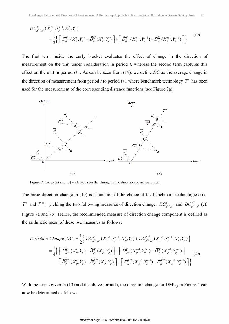
The first term inside the curly bracket evaluates the effect of change in the direction of

measurement on the unit under consideration in period t, whereas the second term captures this

effect on the unit in period t+1. As can be seen from (19), we define DC as the average change in

the direction of measurement from period t to period t+1 where benchmark technology tT has been

used for the measurement of the corresponding distance functions (see Figure 7a).

(a)

(b)

Figure 7. Cases (a) and (b) with focus on the change in the direction of measurement.

The basic direction change in (19) is a function of the choice of the benchmark technologies (i.e. tT and 1tT + ), yielding the two following measures of direction change: 1 ,

t

t tTd d

DC + and 1

1 ,

t

t tTd d

DC+

+ (cf.

Figure 7a and 7b). Hence, the recommended measure of direction change component is defined as

the arithmetic mean of these two measures as follows:

{ }{

1

1 1

1 1

1

1

1 1 1 1, ,

1 1 1 1

1( ) ( , ) ( , )2

1 ( ) ( ) ( ) ( )4

( )

t t

t t t t

t t t t

t t t t

t

t t

T t t t t T t t t tp p p p p p p pd d d d


T t t Tp pd d

Direction Change DC DC X ,Y X ,Y DC X ,Y X ,Y


D X ,Y D

+

+ +

+ +

+

+

+ + + +

+ + + +

= +

= − + −

−

% % % %

% % }1 1 1

11 1 1 1( ) ( ) ( )

t t t

t tt t T t t T t tp p p p p pd d

X ,Y D X ,Y D X ,Y+ + +

++ + + + + −

% %

(20)

With the terms given in (13) and the above formula, the direction change for DMUp in Figure 4 can

now be determined as follows:



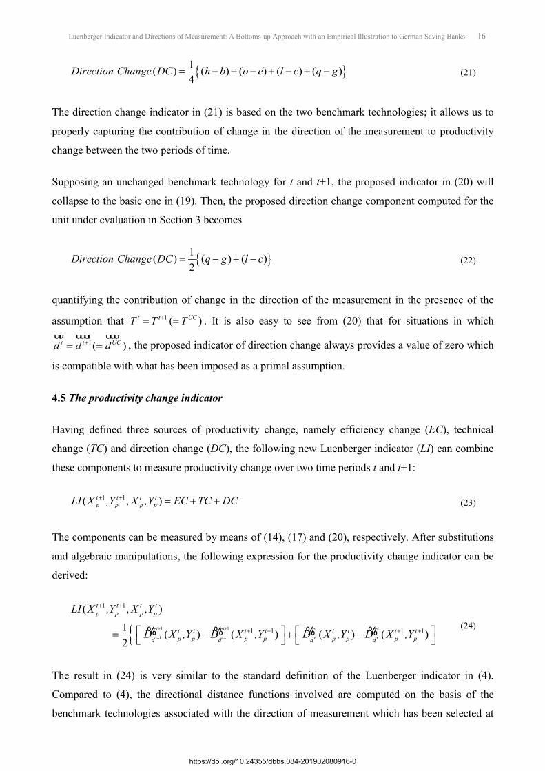
{ }1( ) ( ) ( ) ( ) ( )4

Direction Change DC h b o e l c q g= − + − + − + − (21)

The direction change indicator in (21) is based on the two benchmark technologies; it allows us to

properly capturing the contribution of change in the direction of the measurement to productivity

change between the two periods of time.

Supposing an unchanged benchmark technology for t and t+1, the proposed indicator in (20) will

collapse to the basic one in (19). Then, the proposed direction change component computed for the

unit under evaluation in Section 3 becomes

{ }1( ) ( ) ( )2

Direction Change DC q g l c= − + − (22)

quantifying the contribution of change in the direction of the measurement in the presence of the

assumption that 1 ( )t t UCT T T+= = . It is also easy to see from (20) that for situations in which

1( )t t UCd d d+= =uur uuur uuur

, the proposed indicator of direction change always provides a value of zero which

is compatible with what has been imposed as a primal assumption.

4.5 The productivity change indicator

Having defined three sources of productivity change, namely efficiency change (EC), technical

change (TC) and direction change (DC), the following new Luenberger indicator (LI) can combine

these components to measure productivity change over two time periods t and t+1:

1 1( , )t t t tp p p pLI X ,Y X ,Y EC TC DC+ + = + + (23)

The components can be measured by means of (14), (17) and (20), respectively. After substitutions

and algebraic manipulations, the following expression for the productivity change indicator can be

derived:

{ 1 1

1 1

1 1

1 1 1 1

( , )1 ( ) ( ) ( ) ( )2

t t t t

t t t t

t t t tp p p p


LI X ,Y X ,Y

D X ,Y D X ,Y D X ,Y D X ,Y+ +

+ +

+ +

+ + + + = − + − % % % % (24)

The result in (24) is very similar to the standard definition of the Luenberger indicator in (4).

Compared to (4), the directional distance functions involved are computed on the basis of the

benchmark technologies associated with the direction of measurement which has been selected at



the time. In other words, the direction of measurement kduur

is considered as an element of kT (k = t,

t+1). Consequently, the standard Luenberger indicator in (4) coincides with the proposed measure

of productivity change in (24) where kduur

(resp. 1kd +uuuur

) coupled with kT (resp. 1kT + ) is used in the

computation of the indicator. However, the two-way decomposition and the corresponding

components derived by (4) are not identical with those proposed in this section. It is clear that the

EC and TC components of the two approaches will give the same values if the direction of

measurement remains unchanged over time: the direction change in (20) becomes zero and the

efficiency change and technical change components in (14) and (17) will collapse to the standard

ones given in (5) and (6), respectively.

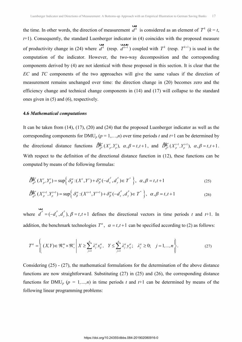
4.6 Mathematical computations

It can be taken from (14), (17), (20) and (24) that the proposed Luenberger indicator as well as the

corresponding components for DMUp (p = 1,…,n) over time periods t and t+1 can be determined by

the directional distance functions ( ), , , 1T t tp pd

D X ,Y t tα

β α β = +% , and 1 1( ), , , 1T t tp pd

D X ,Y t tα

β α β+ + = +% .

With respect to the definition of the directional distance function in (12), these functions can be

computed by means of the following formulas:

{ }( ) sup :( , ) ( , ) , , , 1T t t t tp p x yd

D X ,Y X Y d d T t t= + − ∈ = +%α β β α

βα αβ βd d α β (25)

{ }1 1 1 1( ) sup :( , ) ( , ) , , , 1T t t t tp p x yd

D X ,Y X Y d d T t t+ + + += + − ∈ = +%α β β α

βα αβ βd d α β (26)

where ( , ), , 1x yd d d t t= − = +uur

β β β

β defines the directional vectors in time periods t and t+1. In

addition, the benchmark technologies , , 1T t t= +α α can be specified according to (2) as follows:

1 1( ) ; 0; 1 .

n nm s

j ij j rj jj j

T X,Y X λ x , Y λ y λ j ,...,n+ += =

= ∈ℜ ×ℜ ≥ ≤ ≥ =

∑ ∑α α α α α α (27)

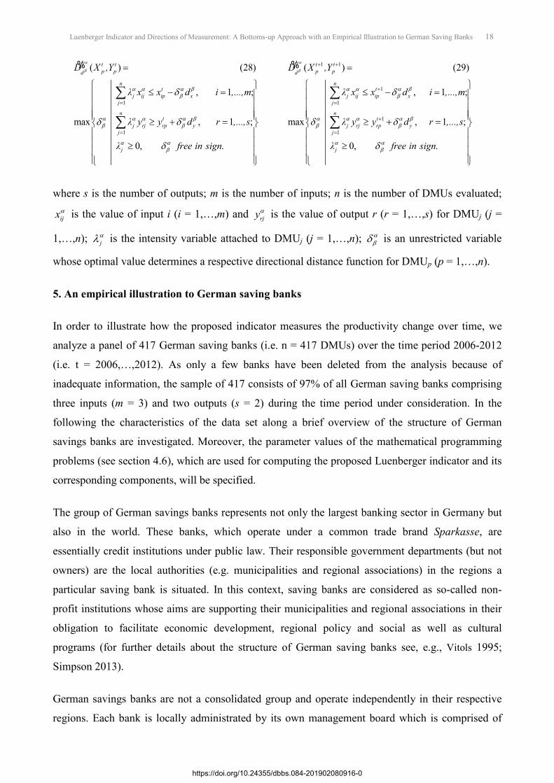
Considering (25) - (27), the mathematical formulations for the determination of the above distance

functions are now straightforward. Substituting (27) in (25) and (26), the corresponding distance

functions for DMUp (p = 1,…,n) in time periods t and t+1 can be determined by means of the

following linear programming problems:



1

1

( ) (28)

, 1 ;

max , 1 ;

0, .

T t tp pd

nt

j ij ip xj

nt

j rj rp yj

j

D X ,Y

λ x x d i ,...,m

λ y y d r ,...,s

λ free in sign

=

=

=

≤ − =

≥ + = ≥

∑

∑

%α

β

α α α ββ

α α α α ββ β

α αβ

d

d d

d

1 1

1

1

1

1

( ) (29)

, 1 ;

max , 1 ;

0, .

T t tp pd

nt

j ij ip xj

nt

j rj rp yj

j

D X ,Y

λ x x d i ,...,m

λ y y d r ,...,s

λ free in sign

+ +

+

=

+

=

=

≤ − =

≥ + = ≥

∑

∑

%α

β

α α α ββ

α α α α ββ β

α αβ

d

d d

d

where s is the number of outputs; m is the number of inputs; n is the number of DMUs evaluated;

ijxα is the value of input i (i = 1,…,m) and rjyα is the value of output r (r = 1,…,s) for DMUj (j =

1,…,n); jαλ is the intensity variable attached to DMUj (j = 1,…,n); α

βd is an unrestricted variable

whose optimal value determines a respective directional distance function for DMUp (p = 1,…,n).

5. An empirical illustration to German saving banks

In order to illustrate how the proposed indicator measures the productivity change over time, we

analyze a panel of 417 German saving banks (i.e. n = 417 DMUs) over the time period 2006-2012

(i.e. t = 2006,…,2012). As only a few banks have been deleted from the analysis because of

inadequate information, the sample of 417 consists of 97% of all German saving banks comprising

three inputs (m = 3) and two outputs (s = 2) during the time period under consideration. In the

following the characteristics of the data set along a brief overview of the structure of German

savings banks are investigated. Moreover, the parameter values of the mathematical programming

problems (see section 4.6), which are used for computing the proposed Luenberger indicator and its

corresponding components, will be specified.

The group of German savings banks represents not only the largest banking sector in Germany but

also in the world. These banks, which operate under a common trade brand Sparkasse, are

essentially credit institutions under public law. Their responsible government departments (but not

owners) are the local authorities (e.g. municipalities and regional associations) in the regions a

particular saving bank is situated. In this context, saving banks are considered as so-called non-

profit institutions whose aims are supporting their municipalities and regional associations in their

obligation to facilitate economic development, regional policy and social as well as cultural

programs (for further details about the structure of German saving banks see, e.g., Vitols 1995;

Simpson 2013).

German savings banks are not a consolidated group and operate independently in their respective

regions. Each bank is locally administrated by its own management board which is comprised of



banking professionals and qualified members. The management board is responsible for the day-to-

day conduct of the business and reporting to a supervisory board of representatives of the

customers, employees and the regional association/council. Furthermore, saving banks are also

controlled centrally by the German Savings Banks Association (Deutscher Sparkassen- und

Giroverband, DSGV) which is the umbrella organization responsible for coordinating decision

making within the group, determining strategic directions, making general policy decisions and

monitoring the activities of the banks to ensure effective and efficient operation with low risk. (see,

e.g., dsgv.de; Simpson 2013).

In the banking literature, productivity measurement and improvement using DEA-based

productivity change indicators/indices have been addressed in many theoretical and application-

oriented studies. An extensive literature review can be found, e.g., in Chen and Yang (2011) as well

as in Paradi and Zhu (2013). In order to measure productivity, input and output factors of banks’

activities must be determined. Two popular approaches have been widely used by researchers, the

production approach and the intermediation approach (Asmild et al. 2004). The production

approach treats banks as producers of products and services such as loans and deposits using labor,

fixed assets and operating expenses. In the intermediation approach, banks are considered as

financial intermediaries, which collect monetary funds from savers/investors and transpose these

funds into further investments. According to these views and based on the data we had access to, we

specified the following inputs and outputs:

• Input #1 (x1): number of employees,

• Input #2 (x2): fixed assets,

• Input #3 (x3): total non-interest expenses,

• Output #1 (y1): total customer deposits,

• Output #2 (y2): total loans.

The selected input and output data have been extracted from the Bankscope database. Descriptive

statistics of the three inputs and two outputs over the time period 2006-2012 are given in Table 1.



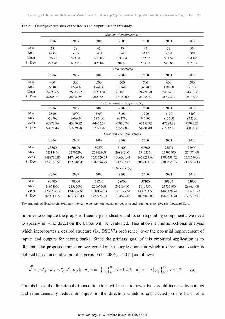
Table 1. Descriptive statistics of the inputs and outputs used in this study.

Number of employees(x1)

2006 2007 2008 2009 2010 2011 2012

Min 39 39 42 39 40 38 39 Max 4785 5328 5434 5547 5622 5724 5891 Mean 525.77 523.34 530.03 533.04 532.53 531.52 531.82

St. Dev. 492.46 498.29 498.04 502.91 508.95 510.86 515.13

Fixed assets(x2)

2006 2007 2008 2009 2010 2011 2012

Min 400 500 500 500 700 600 500 Max 163300 174900 176900 171600 167500 178800 221500 Mean 27690.65 26605.52 25903.84 25343.17 24971.70 24526.86 24386.33

St. Dev. 27525.77 26365.59 26007.50 26190.09 26085.73 25813.39 26138.33

Total non-interest expenses(x3) 2006 2007 2008 2009 2010 2011 2012

Min 2800 3000 2900 3100 3200 3100 3400 Max 650700 660300 658400 694700 747100 813500 842300 Mean 43877.94 45000.72 44462.59 45810.79 45253.72 47389.21 49041.25

St. Dev. 52075.44 52929.78 52277.99 53552.82 54881.49 67232.55 70802.30

Total customer deposits(y1)

2006 2007 2008 2009 2010 2011 2012

Min 83300 86100 89500 94400 95800 95600 97900 Max 22534400 22805200 25543300 26884300 27122300 27392700 27977400 Mean 1418720.86 1478100.96 1551620.38 1606601.44 1658254.68 1700399.52 1751694.96

St. Dev. 1736168.56 1799788.41 1942096.79 2017807.13 2059021.12 2100355.65 2177764.19

Total loans(y2)

2006 2007 2008 2009 2010 2011 2012

Min 69400 70000 61800 58900 57100 59300 63900 Max 21938900 21355600 22667500 24213400 26165500 27730900 29865400 Mean 1286707.19 1299539.81 1338154.68 1361285.61 1405734.53 1465370.74 1513901.92

St. Dev. 1653111.77 1636937.48 1727723.88 1784676.43 1873045.80 1962518.98 2067717.46

The amounts of fixed assets, total non-interest expenses, total customer deposits and total loans are given in thousand Euro.

In order to compute the proposed Luenberger indicator and its corresponding components, we need

to specify in what direction the banks will be evaluated. This allows a multidirectional analysis

which incorporates a desired structure (i.e. DSGV’s preference) over the potential improvement of

inputs and outputs for saving banks. Since the primary goal of this empirical application is to

illustrate the proposed indicator, we consider the simplest case in which a directional vector is

defined based on an ideal point in period t (t = 2006,…,2012) as follows:

{ } { }417 417

1 2 3 1 2 1 1( ; , ); min , 1,2,3; max , 1,2

= == − − − = = = =

uurt t t t t t t t t t

x x x y y xi ij yr rjj jd d , d , d d d d x i d y r (30)

On this basis, the directional distance functions will measure how a bank could increase its outputs

and simultaneously reduce its inputs in the direction which is constructed on the basis of a



hypothetical unit with maximum outputs and minimum inputs in each time period. Values of the

components of the above directional vectors can also be obtained from Table 1. It should be noted

that the idea of the ideal point has also been used in different contexts for the measurement of

efficiency and productivity change (see, e.g., Färe et al. 2004; Portela et al., 2004; Portela and

Thanassoulis 2010).

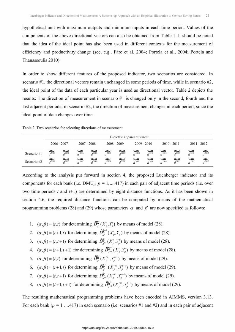
In order to show different features of the proposed indicator, two scenarios are considered. In

scenario #1, the directional vectors remain unchanged in some periods of time, while in scenario #2,

the ideal point of the data of each particular year is used as directional vector. Table 2 depicts the

results: The direction of measurement in scenario #1 is changed only in the second, fourth and the

last adjacent periods; in scenario #2, the direction of measurement changes in each period, since the

ideal point of data changes over time.

Table 2. Two scenarios for selecting directions of measurement.

Directions of measurement

2006 - 2007 2007 - 2008 2008 - 2009 2009 - 2010 2010 - 2011 2011 - 2012

Scenario #1 2006duuuur

2006duuuur

2006duuuur

2008duuuur

2008duuuur

2008duuuur

2008duuuur

2010duuuur

2010duuuur

2010duuuur

2010duuuur

2012duuuur

Scenario #2 2006duuuur

2007duuuur

2007duuuur

2008duuuur

2008duuuur

2009duuuur

2009duuuur

2010duuuur

2010duuuur

2011duuuur

2011duuuur

2012duuuur

According to the analysis put forward in section 4, the proposed Luenberger indicator and its

components for each bank (i.e. DMUp; p = 1,…,417) in each pair of adjacent time periods (i.e. over

two time periods t and t+1) are determined by eight distance functions. As it has been shown in

section 4.6, the required distance functions can be computed by means of the mathematical

programming problems (28) and (29) whose parameters α and β are now specified as follows:

1. ( ) ( , )α β =, t t for determining ( )%t

tT t t

p pdD X ,Y by means of model (28).

2. ( ) ( 1, )α β = +, t t for determining 1

( )t

tT t t

p pdD X ,Y

+% by means of model (28).

3. ( ) ( , 1)α β = +, t t for determining 1 ( )t

tT t t

p pdD X ,Y+% by means of model (28).

4. ( ) ( 1, 1)α β = + +, t t for determining 1

1 ( )t

tT t t

p pdD X ,Y

+

+% by means of model (28).

5. ( ) ( , )α β =, t t for determining 1 1( )+ +%t

tT t t


6. ( ) ( 1, )α β = +, t t for determining 1 1 1( )

t

tT t t

p pdD X ,Y

+ + +% by means of model (29).

7. ( ) ( , 1)α β = +, t t for determining 11 1( )

t

tT t t

p pdD X ,Y+

+ +% by means of model (29).

8. ( ) ( 1, 1)α β = + +, t t for determining 1

11 1( )

+

++ +%t

tT t t


The resulting mathematical programming problems have been encoded in AIMMS, version 3.13.

For each bank (p = 1,…,417) in each scenario (i.e. scenarios #1 and #2) and in each pair of adjacent



time periods (i.e. 2006-07, 2007-08, 2008-09, 2009-10, 2010-11, 2011-12) the above eight distance

functions have been calculated. Thus, in total (417×2×6×8 =) 40032 linear programming problems

have been solved. The results have subsequently been used to determine the proposed Luenberger

indicator and its components for each bank in each scenario and in each pair of adjacent time

periods as follows:

• Efficiency change (EC) component has been determined by applying formula (14) on the

basis of the results of the distance functions in (1) and (8),

• Technical change (TC) component has been determined by applying formula (17) on the

basis of the results of the distance functions in (1), (2), (4), (5), (6), (7) and (8),

• Direction change (DC) component has been determined by applying formula (20) on the

basis of the results of the distance functions in (1)-(8),

• The Luenberger indicator (LI) has been determined by applying formula (24) on the basis of

the results of the distance functions in (1), (4), (5) and (8).

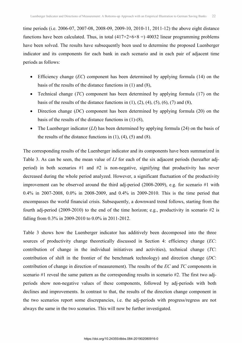
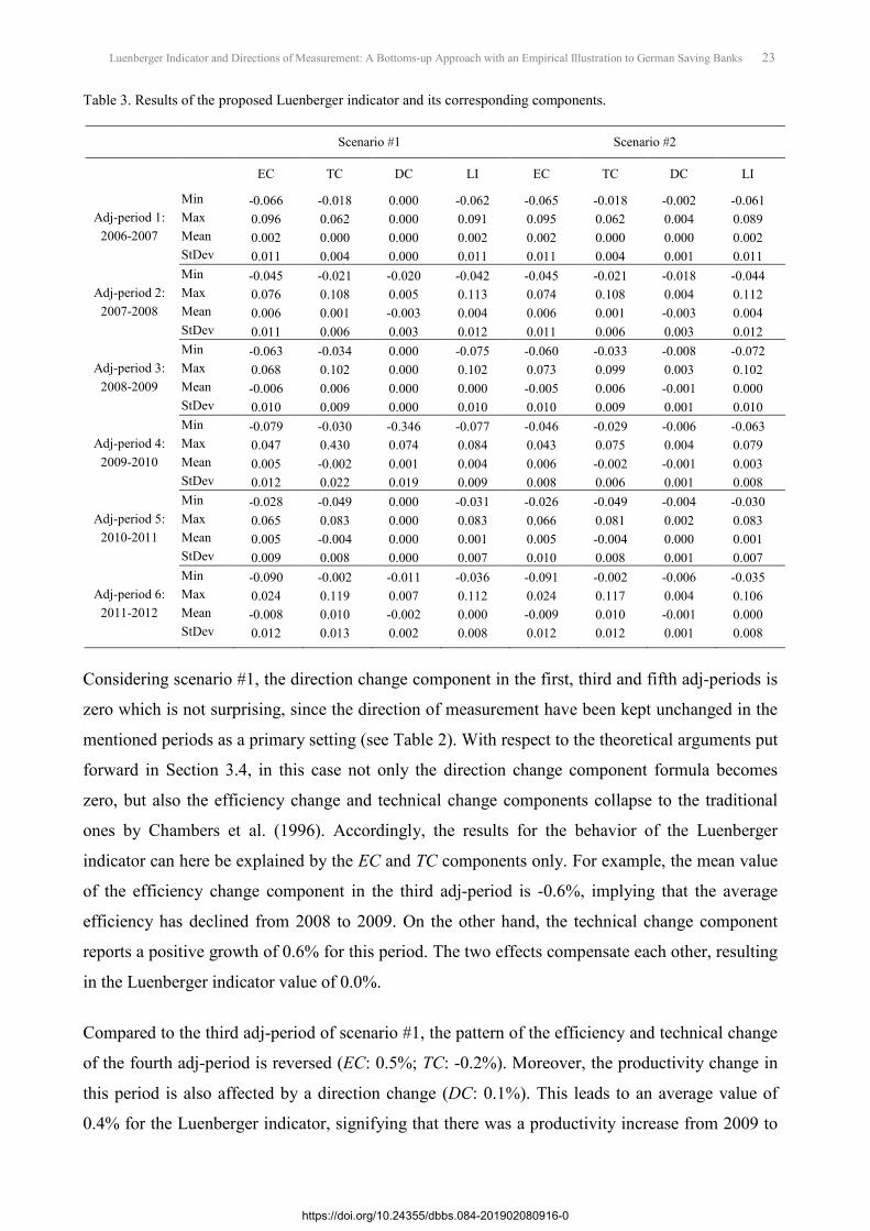
The corresponding results of the Luenberger indicator and its components have been summarized in

Table 3. As can be seen, the mean value of LI for each of the six adjacent periods (hereafter adj-

period) in both scenarios #1 and #2 is non-negative, signifying that productivity has never

decreased during the whole period analyzed. However, a significant fluctuation of the productivity

improvement can be observed around the third adj-period (2008-2009), e.g. for scenario #1 with

0.4% in 2007-2008, 0.0% in 2008-2009, and 0.4% in 2009-2010. This is the time period that

encompasses the world financial crisis. Subsequently, a downward trend follows, starting from the

fourth adj-period (2009-2010) to the end of the time horizon; e.g., productivity in scenario #2 is

falling from 0.3% in 2009-2010 to 0.0% in 2011-2012.

Table 3 shows how the Luenberger indicator has additively been decomposed into the three

sources of productivity change theoretically discussed in Section 4: efficiency change (EC:

contribution of change in the individual initiatives and activities), technical change (TC:

contribution of shift in the frontier of the benchmark technology) and direction change (DC:

contribution of change in direction of measurement). The results of the EC and TC components in

scenario #1 reveal the same pattern as the corresponding results in scenario #2. The first two adj-

periods show non-negative values of these components, followed by adj-periods with both

declines and improvements. In contrast to that, the results of the direction change component in

the two scenarios report some discrepancies, i.e. the adj-periods with progress/regress are not

always the same in the two scenarios. This will now be further investigated.



Table 3. Results of the proposed Luenberger indicator and its corresponding components.

Scenario #1 Scenario #2

EC TC DC LI EC TC DC LI

Min -0.066 -0.018 0.000 -0.062 -0.065 -0.018 -0.002 -0.061 Adj-period 1: Max 0.096 0.062 0.000 0.091 0.095 0.062 0.004 0.089

2006-2007 Mean 0.002 0.000 0.000 0.002 0.002 0.000 0.000 0.002 StDev 0.011 0.004 0.000 0.011 0.011 0.004 0.001 0.011 Min -0.045 -0.021 -0.020 -0.042 -0.045 -0.021 -0.018 -0.044

Adj-period 2: Max 0.076 0.108 0.005 0.113 0.074 0.108 0.004 0.112 2007-2008 Mean 0.006 0.001 -0.003 0.004 0.006 0.001 -0.003 0.004

StDev 0.011 0.006 0.003 0.012 0.011 0.006 0.003 0.012 Min -0.063 -0.034 0.000 -0.075 -0.060 -0.033 -0.008 -0.072

Adj-period 3: Max 0.068 0.102 0.000 0.102 0.073 0.099 0.003 0.102 2008-2009 Mean -0.006 0.006 0.000 0.000 -0.005 0.006 -0.001 0.000

StDev 0.010 0.009 0.000 0.010 0.010 0.009 0.001 0.010 Min -0.079 -0.030 -0.346 -0.077 -0.046 -0.029 -0.006 -0.063

Adj-period 4: Max 0.047 0.430 0.074 0.084 0.043 0.075 0.004 0.079 2009-2010 Mean 0.005 -0.002 0.001 0.004 0.006 -0.002 -0.001 0.003

StDev 0.012 0.022 0.019 0.009 0.008 0.006 0.001 0.008 Min -0.028 -0.049 0.000 -0.031 -0.026 -0.049 -0.004 -0.030

Adj-period 5: Max 0.065 0.083 0.000 0.083 0.066 0.081 0.002 0.083 2010-2011 Mean 0.005 -0.004 0.000 0.001 0.005 -0.004 0.000 0.001

StDev 0.009 0.008 0.000 0.007 0.010 0.008 0.001 0.007 Min -0.090 -0.002 -0.011 -0.036 -0.091 -0.002 -0.006 -0.035

Adj-period 6: Max 0.024 0.119 0.007 0.112 0.024 0.117 0.004 0.106 2011-2012 Mean -0.008 0.010 -0.002 0.000 -0.009 0.010 -0.001 0.000

StDev 0.012 0.013 0.002 0.008 0.012 0.012 0.001 0.008

Considering scenario #1, the direction change component in the first, third and fifth adj-periods is

zero which is not surprising, since the direction of measurement have been kept unchanged in the

mentioned periods as a primary setting (see Table 2). With respect to the theoretical arguments put

forward in Section 3.4, in this case not only the direction change component formula becomes

zero, but also the efficiency change and technical change components collapse to the traditional

ones by Chambers et al. (1996). Accordingly, the results for the behavior of the Luenberger

indicator can here be explained by the EC and TC components only. For example, the mean value

of the efficiency change component in the third adj-period is -0.6%, implying that the average

efficiency has declined from 2008 to 2009. On the other hand, the technical change component

reports a positive growth of 0.6% for this period. The two effects compensate each other, resulting

in the Luenberger indicator value of 0.0%.

Compared to the third adj-period of scenario #1, the pattern of the efficiency and technical change

of the fourth adj-period is reversed (EC: 0.5%; TC: -0.2%). Moreover, the productivity change in

this period is also affected by a direction change (DC: 0.1%). This leads to an average value of

0.4% for the Luenberger indicator, signifying that there was a productivity increase from 2009 to



2010. As can be seen in scenario #2 for the same adj-period, the result of the technical change

component is identical to the one obtained in scenario #1. However, the efficiency change

component in the second scenario is 0.1% higher than in the first scenario. In addition, the

direction change component signals a negative value of -0.1% in scenario #2, which is reversed

compared to its value in scenario #1. This is due to the fact that the productivity change indicators

of the two scenarios apply different directional vectors for the computation of the directional

distance functions (cf. Table 2).

Scenario #2 reveals another aspect of the impact of the change in direction of measurement on the

results of the productivity over time. During the periods analyzed, the direction change component

reports negative values with the exception in the first (2006-2007) and fifth (2009-2010) adj-

periods whose mean values of the direction change components are zero. Looking at the fifth

period, e.g., the direction of measurement has been changed from 2010 to 2011 as a primary

setting (see Table 2). Although the effect of this change on the results of the productivity varies

between (Min:) -0.4% and (Max:) 0.2%, its mean value amounts to zero. This means that the

average productivity change of 0.1% in this period can mostly be explained by considering the

effect of the other components, i.e. of EC and TC: the amount of the technical change component

in this period is -0.4% on average which captures a negative shift in the frontier of the benchmark

technology from 2010 to 2011; however, the average efficiency has changed positively over this

period by a value of 0.5% which results to the positive rate of growth of 0.1% in productivity.

It should be noted that the inefficiency of a unit has been defined as the maximum expansion in

outputs and/or contraction in inputs along the predetermined direction of measurement. Therefore,

change in efficiency as well as in the direction component will be zero for a bank which has been

efficient in time periods t and t+1. In other words, such a bank not only remains a best practice

unit but also any change in direction of measurement does not affect its productivity. A closer look

at the results in general in both scenarios shows that four banks have been efficient in all time

periods. Consequently, the direction change component for these banks is zero in all periods;

compared to other, inefficient banks, that their performance has been less sensitive to changes in

the direction of measurement over the selected periods.

6. Conclusions and Outlook on Future Research

The Luenberger indicator applies directional distance functions which allow to specifying in what

direction (i.e. direction of measurement) the operating units will be evaluated. Within this

framework, the performance of a unit is characterized by measuring the distance to the boundary



of the benchmark technology along the predetermined direction of measurement, i.e. a directed

distance is defined. Arising from a series of practical cases, in multiple time period analysis not

only the shape and the characteristics of the benchmark technology may change (e.g., due to

policy directives, the competitive situation and economic conditions), but also the direction of

measurement. However, the existing Luenberger indicator is unable to distinguish between these

two sources of productivity changes. Consequently, in the presence of a change in the direction of

measurement, the standard components of the indicator may provide values which are not

compatible with reality.

In order to overcome the above-described problem, we have revisited the Luenberger indicator

and its components. Making use of the bottoms-up approach, we started with a list of selected

sources of productivity change, namely efficiency change, technical change and direction change.

We then examined the best possible way of measuring each of these sources and combined them

to derive a new measure of productivity change. The new indicator does not only measure

efficiency change and technical change components in an appropriate way, but is also able to

capture the degree to which predetermined directions of measurement affect the productivity of

units over time.

The proposed framework is suitable especially for situations where some variables are controlled

by the central management of an organization which supervises the operating units. In such cases,

a preferred direction of measurement can be determined with regard to the corporate strategy and

overall goals of the organization. This direction is usually beyond the control of local managers

and may change over time. On this basis, any change in the direction of measurement can force

the operating units to adapt their local variables (e.g., local strategy, scale of operation etc.) in

order to avoid their productivity to be affected over time. Hence, the proposed framework can be

used as a managerial control instrument to provide managers and policymakers with information

to help them design better strategies aimed at achieving sustainable productivity growth.

In order to illustrate how the proposed Luenberger indicator measures the productivity change

over time, a panel of 417 German saving banks over the time period 2006-2012 has been

analyzed. In order to show different features of the proposed indicator, two scenarios for

specifying the directions of measurement (i.e. DSGV’s preference over the potential improvement

of inputs and outputs) have been considered. The results demonstrated how the proposed approach

is able to properly measure efficiency change and technical change, revealing effects of the change

in direction of measurement on the results of the productivity over time. Moreover, a comparison

of the results of both scenarios verified that the components of the Luenberger indicator may



change by different assumptions made about the directions of measurement over time. This

highlights the fact that apart from efficiency change and technical change as two standard drivers

of productivity change, any regress or progress in the productivity of a unit can be explained by

considering the change in the direction of measurement.

The productivity indicators suggested in the literature have different properties and features.

Depending on a specific situation with certain assumptions, it has to be decided which kind of

indicator could be superior to the others. In this context, an interesting perspective for future

research is to apply the proposed approach to other types of productivity change indicators which

use an inter-temporal structure in their nature. An example is the sequential Malmquist index in

which a sequential technology is formed from convex aggregation of observations in all periods

up to the period under consideration (see, e.g., Shestalova 2003). Another example is the meta-

frontier approach with an additional inter-temporal benchmark technology which is the convex

union of some contemporaneous benchmark technologies (see, e.g., Battese et al. 2004).

References

Aghdam, R.F, 2011. Dynamics of productivity change in the Australian electricity industry: Assessing the impacts of electricity reform. Energy Policy, 39, 3281-3295.

Ahn, H., Neumann, L., and Novoa, N.V, 2012. Measuring the relative balance of DMUs. European Journal of Operational Research, 221, 417-423.

Aparicio, J., Pastor, J.T., and Zofio, J.L, 2013. On the inconsistency of the Malmquist–Luenberger index. European Journal of Operational Research, 229, 738-742.

Asmild. M., Paradi, J.C., Aggarwall, V., and Schaffnit, C, 2004. Combining DEA window analysis with the Malmquist index approach in a study of the Canadian banking industry. Journal of Productivity Analysis, 21, 67-89.

Asmild, M., Paradi, J.C., and Pastor, J.T, 2009. Centralized resource allocation BCC models. Omega, 37, 40-49.

Athanassopoulos, A.D, 1995. Goal programming & data envelopment analysis (GoDEA) for target-based multi-level planning: Allocating central grants to the Greek local authorities. European Journal of Operational Research, 18, 535-550.

Balk, B.M, 2001. Scale efficiency and productivity change. Journal of Productivity Analysis, 15, 159-183.

Banker, R.D., Charnes, A., and Cooper, W.W, 1984. Some models for estimating technical and scale inefficiency in Data Envelopment Analysis. Management Science, 31, 1078-1092.

Battese, G.E., Rao, D.S.P., and Donnell, C.J, 2004. A metafrontier production function for estimation of technical efficiencies and technology gaps for firms operating under different technologies. Journal of Productivity Analysis, 21, 91-103.



Berg, S.A., Førsund, F.R., and Jansen, E.S, 1992. Malmquist indexes of productivity growth during the deregulation of Norwegian banking 1980-1989. The Scandinavian Journal of Economics, 94, 211-228.

Bogetoft, P., and Otto, L, 2011. Benchmarking with DEA, SFA, and R. Springer, New York.

Caves, D.W., Christensen, L.R., and Dievert, W.E, 1982. The economic theory of index number and the measurement of input output and productivity. Econometrica, 50, 1393-1414.

Chambers, R.G., Chung, Y., and Färe, R, 1998. Profit, directional distance functions, and nerlovian efficiency. Journal of Optimization Theory and Applications, 98, 351-364.

Chambers, R.G., Färe, R., Grosskopf, S, 1996. Productivity growth in APEC countries. Pacific Economic Review, 1, 181-190.

Charnes, A., Cooper, W.W., and Rhodes, E, 1978. Measuring the efficiency of the decision making units. European Journal of Operational Research, 2, 429-444.

Chen, Y, 2003. A Non-radial Malmquist productivity index with an illustrative application to Chinese major industries. International Journal of Production Economics, 83, 27-35.

Chowdhury, H., Wodchis, W., and Laporte, A, 2011. Efficiency and technological change in health care services in Ontario: An application of Malmquist productivity index with bootstrapping. International Journal of Productivity and Performance Management, 60, 721-745.

Chung, Y., Färe, R., and Grosskopf, S, 1997. Productivity and undesirable outputs: A directional distance function approach. Journal of Environmental Management, 51, 229-240.

Cook, W.D., and Zhu, J, 2007. Within-group common weights in DEA: An analysis of power plant efficiency. European Journal of Operational Research, 178, 207-216.

Corton, M.L., and Berg, S.V, 2009. Benchmarking central American water utilities. Utilities Policy, 17, 267-275.

DSGV (Deutscher Sparkassen- und Giroverband) 2013. Missions & objectives. http://www.dsgv.de/en/about-us/index.html. Accessed 12.10.2013.

Fang, L, 2013. A generalized DEA model for centralized resource allocation. European Journal of Operational Research, 228, 405-412.

Färe, R., and Grosskopf, S, 2000. Theory and application of directional distance functions. Journal of Productivity Analysis, 13, 93-103.

Färe, R., Grosskopf, S., and Hernadez-Sancho, F, 2004. Environmental performance: An index number approach. Resource and Energy Economics, 26, 343-352.

Färe, R., Grosskopf, S., Lindgren, B., and Roos, P, 1992. Productivity developments in Swedish hospitals: A non-parametric Malmquist approach. Journal of Productivity Analysis, 3, 85-101.

Färe, R., Grosskopf, S., Norris, M., and Zhang, Z, 1994. Productivity growth, technical progress, and efficiency changes in industrialized countries. The American Economic Review, 84, 66-83.

Farrell, J.M, 1957. The measurement of productivity efficiency. Journal of the Royal Statistical Society, 120, 253-290.



Gilbert, R.A., and Wilson, P, 1998. Effects of deregulation on the productivity of Korean banks. Journal of Economics and Business. 50, 133-155.

Gitto, S., and Mancuso, P, 2012. Bootstrapping the Malmquist indexes for Italian airports. International Journal of Production Economics, 135, 403-411.

Grifell-Tatje, E., and Lovell, C.A.K, 1999. Profits and productivity. Management Science, 45, 1177-1193.

Grifell-Tatje, E., Lovell, C.A.K., and Pastor, J.T, 1998. A quasi-Malmquist productivity index. Journal of Productivity Analysis, 10, 7-20.

Grosskopf, S, 1986. The role of the reference technology in measuring productive efficiency. The Economic Journal, 96, 499-513.

Grosskopf , S, 2003. Some remarks on productivity and its decompositions. Journal of Productivity Analysis, 20, 459-474.

Hisali, E., and Yawe, B, 2011. Total factor productivity growth in Uganda’s telecommunications industry. Telecommunications Policy, 35, 12-19.

Kao, C, 2010. Malmquist productivity index based on common-weights DEA: The case of Taiwan forests after reorganization. Omega, 38, 484-491.

Kirigia, J.M., Emrouznejad, A., Cassoma, B., Asbu, E.Z., and Barry, S, 2008. A performance assessment method for hospitals: The case of municipal hospitals in Angola. Journal of Medical Systems, 32, 509-519.

Lam, P., and Shiu, A, 2010. Economic growth telecommunications development and productivity growth of the telecommunications sector: Evidence around the world. Telecommunications Policy, 34, 185-199.

Langfield-Smith, K, 1997. Management control systems and strategy: A critical review. Accounting, Organizations and Society, 22, 207-232.

Li, S.K., and Ng, Y.C, 1995. Measuring the productive efficiency of a group of firms. International Advances in Economic Research, 1, 377-390.

Lozano, S., and Villa, G, 2004. Centralized resource allocation using data envelopment analysis. Journal of Productivity Analysis, 22, 143-161.

Nishimizu, M., and Page, J.M, 1982. Total factor productivity growth, technological progress and technical efficiency change: Dimensions of productivity change in Yugoslavia, 1967-1978. The Economic Journal, 92, 920-936.

Nudurupati, S.S., Bititci, U.S., Kumar, V., and Chan, F.T.S, 2011. State of the art literature review on performance measurement. Computers & Industrial Engineering 60, 279-290.

Paradi, J.C., and Zhu, H, 2013. A survey on bank branch efficiency and performance research with Data Envelopment Analysis. Omega, 41, 61-79.

Park, K.H., and Weber, W.L, 2006. A note on efficiency and productivity growth in the Korean banking industry, 1992–2002. Journal of Banking & Finance, 30, 2371-2386.

Pastor, J.T., Asmild, M., and Lovell, C.A, 2011. The biennial Malmquist productivity change index. Socio-Economic Planning Sciences, 45, 210-15.



Pastor, J.T., and Lovell, C.A, 2005. A global Malmquist productivity index. Economics Letters, 88, 266-271.

Pires, H.M., and Fernandes, E, 2012. Malmquist financial efficiency analysis for airlines. Transportation Research Part E, 48, 1049-1055.

Portela, M.C.A.S., and Thanassoulis, E, 2010. Malmquist-type indices in the presence of negative data: An application to bank branches. Journal of Banking & Finance, 34, 1472-1483.

Portela, M.C.A.S., Thanassoulis, E., and Simpson, G, 2004. Negative data in DEA: A directional distance approach applied to bank branches. Journal of the Operational Research Society, 55, 1111-1121.

Portela, M.C.A.S., Thanassoulis, E., Horncastle, A., and Maugg, T, 2011. Productivity change in the water industry in England and Wales: Application of the meta-Malmquist index. Journal of the Operational Research Society, 62, 2173-2188.

Ray, S.C., and Desli, E, 1997. Productivity growth, technical progress and efficiency change in industrialized countries: Comment. The American Economic Review, 87, 1033-1039.

Shestalova, V, 2003. Sequential Malmquist indices of productivity growth: An application to OECD industrial activities. Journal of Productivity Analysis, 19, 211-226.

Simpson, C.V.J, 2013. The German Sparkassen (savings banks): A commentary and case study. Civitas, London.

Tovar. B., Ramos-Real, F.J., and Fagundes, de Almeida E, 2011. Firm size and productivity: Evidence from the electricity distribution industry in Brazil. Energy Policy, 39, 826-833.

Vitols, S, 1995. German banks and the modernization of the small firm sector: Long-term finance in comparative perspective. WZB Labor Market and Employment, Working paper No. FS I 95-309.

Wheelock, D.C., and Wilson, P, 1999. Technical progress, inefficiency and productivity change in U.S. banking 1984-1993. Journal of Money, Credit and Banking, 31, 212-234.

Xu, L, 2012. Theoretical and empirical studies of productivity growth in the agricultural economics: Cases of China and the United States. Physics Procedia, 24, 1475-1481.


http://www.wiley.com/bw/journal.asp?ref=0022-2879

Documents

Luenberger Indicator and Directions of Measurement: A