Embed Size (px)
Citation preview

SPWLA 47th Annual Logging Symposium, June 4-7, 2006
1
LWD DENSITY RESPONSE TO BED LAMINATIONS IN HORIZONTAL AND VERTICAL WELLS
R. J. Radtke, Mike Evans, and John C. Rasmus, Schlumberger, Darwin V. Ellis, Joseph M.
Chiaramonte, and Charles R. Case, Schlumberger-Doll Research, and Ed Stockhausen, Chevron
Copyright 2006, held jointly by the Society of Petrophysicists and Well Log Analysts (SPWLA) and the submitting authors.
This paper was prepared for presentation at the SPWLA 47 th Annual Logging Symposium held in Veracruz, Mexico, June 4 -7, 2006.
ABSTRACT Despite the increasing prevalence of thinly bedded reservoirs, questions relating to the response of nuclear LWD tools in such fields have gone largely unanswered in the literature. Motivated by specific anomalies in well logs from a field in West Africa, response modeling of a commercial LWD density tool in a layered medium was performed to answer some of these questions. A rich variety of responses was revealed. In a vertical well, an axial geometric factor, the scale of which was set by the source-to-detector distance, determines the response. For layers thinner than this scale, the measured density does not represent the true bed density of the individual layers. In fact, for layers much thinner than this scale, the measured density is the average of the densities of the individual layers. In horizontal wells, a radial geometrical factor governs the response. Although also related to the source-to-detector distance, the scale of the radial geometrical factor is much smaller than that of the axial geometric factor. Consequently, the density measurement in horizontal wells is able to resolve much thinner beds than in vertical wells. Field examples of the LWD tool response to bed laminations in a horizontal well are presented that verify the principles learned from the modeling. Comparisons of the vertical wireline (WL) log response with the horizontal LWD log response reveal the layer geometries in which these logs provide the formation density directly and the layer geometries in which advanced processing and/or modeling are required. The examples confirm that the LWD density logs in high-angle wells can read the true bed density in much thinner beds than a density log in a vertical well can. The result is a more accurate determination of layer porosities, net pay, and hydrocarbons in place.
INTRODUCTION Increasingly, formation evaluation measurements are obtained from LWD tools in high-angle and horizontal wells rather than from traditional W L tools in vertical wells. Questions often aris e as to how the geometrical effects of crossing layers of beds with varying thicknesses and properties will affect these measurements (Passey, 2005). Only a limited number of publications have dealt with the geometrical effects on nuclear measurements in high-angle and horizontal wells (see, for example, Ellis and Chiaramonte, 2000). These issues were brought into focus recently during the development of a field in West Africa. It was observed that the density porosity obtained from LWD tools in horizontal and high-angle wells matched the core porosity better than WL densities obtained from vertical wells. Since the density measurements are very similar between LWD and WL tools, the most likely explanation for this discrepancy involves the difference between tool responses in vertical and horizontal wells. This paper explores this response difference through an extensive modeling program based on one of the commercial LWD density tools used in this particular field. The modeling results are used to explain some of the logs from this field. The conclusions from this study justify updating the reservoir properties based on the density log measurements in the horizontal and high-angle wells. RESPONSE MODELING The LWD tool used was the same one used for some of the field logs that motivated this study. This tool is nominally a 6.75-in API collar tool, but in these wells a version of the tool having an 8.25-in integral-blade stabilizer over the density section was used. The tool is assumed to be fully eccentered against the formation, as is typically the case for even a minor deviation of the borehole from the vertical. The bit size is 8.5 in. Consequently, the presence of the stabilizer on the tool reduces the difference between ZZ

SPWLA 47th Annual Logging Symposium, June 4-7, 2006
2
the borehole and tool diameters, thereby improving the density measurements and images. For simplicity, the drilling fluid is assumed to be fresh water when modeling the bed laminations. The formations studied were laminations of geological layers with alternating densities. The compositions of these layers are taken from core samples from the field and are summarized in Table 1. In particular, note that the low-density layer has a density of 2.0 g/cm3 and the high-density layer has a density of 2.6 g/cm3. The formations are alternating equal-thickness beds of these materials.
Table 1 Compositions, densities, and photoelectric factors (PE’s) of the materials used in the modeling.
Parameter Low-
Density Bed High-
Density Bed Composition (m3/ m3) Quartz Calcite Illite Water Density (g/cm3) Pe
60 0 0 40
2.00 1.49
62 30 4 4
2.60 2.91
The density response is modeled in detail to reproduce the response that would occur using this tool in the conditions examined. The modeling may be broken down into two parts: the first simulates the physical response of the density tool and the second simulates the interpretation of the measured count rates as a function of density. The physical response of the density tool was separated into the parts shown on the left side of Figure 1. Gamma rays from the 137Cs source in the tool are emitted and travel into the tool, borehole, and formation. Some of these gamma rays are scattered into the detectors, where they interact with the detector material (the scintillator NaI(Th) in this tool) to produce light. The light is converted into electrons and amplified by the photomultiplier tube (PMT). Electronics then further amplify and condition the signal, yielding an electrical pulse for each detected gamma ray with an amplitude related to the energy of the incident gamma ray. These pulses are collected into a pulse-height spectrum. This process is simulated as indicated on the right side of Figure 1. Tracking the gamma rays from source to detector is accomplished using the industry-standard Monte Carlo N-Particle (MCNP) transport code developed by Los Alamos National Laboratory (Girard, 2005). The MCNP model employed is the
same one used for the design and response characterization of the tool. Translating a gamma ray incident on a detector into a pulse height is achieved through the code GAMRES (Evans, 1981). This is an analog Monte Carlo code, also developed at Los Alamos National Laboratory, which includes the effects of down-scattering of the gamma rays in the detector, the near-detector environment, the slight nonlinearity in light output of the NaI(Th) scintillator, and the broadening effects of the PMT and pulse-shaping electronics. GAMRES produces a response map that relates incident gamma rays of a specific energy to a pulse height spectrum. Convolving the MCNP-computed particle current into the detectors with the appropriate GAMRES response map produces the final pulse-height spectra. The final, critical step in simulating the physical response of the density tool is to extract the window count rates. It has been recognized for some time (Bertozzi, Evans, and Wahl, 1981; Ellis et al., 1985; and Ellis , 1987) that the high-energy part of the pulse-height spectrum is most sensitive to formation density, while the low-energy part is most sensitive to lithology. For this reason, most modern density tools integrate the pulse-height spectra over at least two windows, one of which covers the high-energy, density-dominated regime while the other covers the low-energy, lithology-dominated regime. Simply summing the pulse-height spectra into total count rates mixes these sensitivities and produces a sub-optimal response. In the calculations presented here, the boundaries of the energy windows used in the model are the same as those used in the actual tool. The interpretation of the window count rates as a density is the second part of the modeling and is summarized in Figure 1. The interpretation algorithm used to proces s the modeling results is the same as that used in the commercial software available for this tool. In both instances, the window count rates are first depth- and resolution-matched to eliminate any nonphysical response caused by differences in the detector measure points and vertical resolutions (see, for example, Flaum et al., 1987). The window count rates are then calibrated to measurements in aluminum and magnesium alloy blocks made in the shop before the logging job. This calibration removes the effects of source-to-source and tool-to-tool variations and also compensates for the effects of tool wear. The calibrated window count rates are run through a standard spine-and-rib-type algorithm used in WL tools (Ellis et al., 1985; Ellis , 1987). In this algorithm, an apparent density is computed for the

SPWLA 47th Annual Logging Symposium, June 4-7, 2006
3
detector closer to the source, the short-spaced density ρS, and for the detector farther from the source, the long-spaced density ρL. The apparent densities have been corrected for the small effects of photoelectric absorption not eliminated by selecting the high-energy part of the pulse-height spectrum. A larger and more important correction is the rib correction ∆ρ, which compensates for standoff and mud cake between the tool and the formation. This correction is derived from the difference between ρS and ρL and is approximately linear when this difference is small, as shown in
SL ρρρ −∝∆ . (1)
The compensated density ρb is obtained by adding this correction to the LS density in
ρρρ ∆+= Lb . (2)
The compensated density is the conventional density presented in density logs. The processing just described is the standard processing. It provides a very accurate density at each depth, and its vertical resolution is determined by the distance between the source and the long-spaced detector. In laminated formations, it is often desirable to obtain the best vertical resolution possible. An improved vertical resolution can be obtained from the short-spaced detector because of its lesser distance from the source. However, a means of compensating for tool standoff must be derived to preserve the accuracy of the result. One method for achieving this goal is referred to as alpha processing (Flaum, Galford, and Hastings, 1987). At each depth, a correction to ρS is applied based on the difference between ρb and ρS averaged over a long depth interval, typically approximately 4 ft. The resulting alpha-processed density has an enhanced vertical resolution and an average accuracy that is the same as ρb. The algorithms detailed above apply equally well to WL and LWD density tools. One peculiarity of LWD density tools is that they often rotate during the measurement. Because gravity tends to pull the tool to the bottom of the borehole, this rotation is accommodated by recording the count rates as a function of the azimuthal orientation of the tool. Then, the density obtained is reported when the detectors are in the bottom quadrant of the borehole. Specifically, the tool used divides the circumference of the borehole into 16 sectors and accumulates count rates in each sector. These sector count rates are used to derive sector densities as described above, and the bottom four sector densities are averaged to produce a bottom-quadrant density. The bottom-quadrant density is usually the most representative of the
formation and therefore is the one commonly plotted in the logs. Explicit calculations show that rotational effects are not significant in the vertical well geometry studied, but they can be significant in the horizontal wells. Consequently, the modeling results reported for the horizontal wells include the rotational effects. For each configuration, the model is run for four different azimuthal orientations of the tool, and the results are averaged to produce sector count rates. These sector count rates are then processed to produce the bottom-quadrant densities reported. To determine how well the model reproduces the actual tool response, several test cases were computed in homogeneous formations. The formations are the magnesium and aluminum alloy calibration blocks, the low- and high-density materials from Table 1, a 50% -50% volumetric mixture of the two materials from Table 1 at a density of 2.3 g/cm3, and a 2.3 g/cm3 Berea sandstone. The results are summarized in Figure 3. We first calculated the response with the tool fully eccentered against the formation (the blue points in Figure 3). The short-spaced, long-spaced, and compensated densities produced by the model are all given to within the accuracy specifications of this tool, ±0.015 g/cm3. These res ults confirm that the model correctly reproduces the density in the range of interest. The proper reproduction of the correction for standoff and mud cake is shown by the orange and red points in Figure 3. In these computations, the tool is stood off from the formation 1/8 in, and the borehole fluid is replaced by 1.19 g/cm3 barite-loaded water-based mud (orange points) or 2.53 g/cm3 barite-loaded water-based mud (red points). For both fluids, the short-spaced (Figure 3, panel a) and long-spaced (Figure 3, panel b) densities deviate from their bulk values as expected when the tool is separated from the formation. The light mud decreases the apparent density and the heavy mud increases it. This effect is larger in the short-spaced density compared to the long-spaced density because of the reduced depth-of-investigation resulting from the short-spaced detector’s smaller separation from the source. The effect is also larger as the density contrast between the mud and the formation increases; i.e., the magnitude of the density error is largest for the heavy mud in the light formation and the light mud in the heavy formation. Consistent with these observations, the density correction (Figure 3, panel c) is positive for the light mud and negative for the heavy mud and ZZ
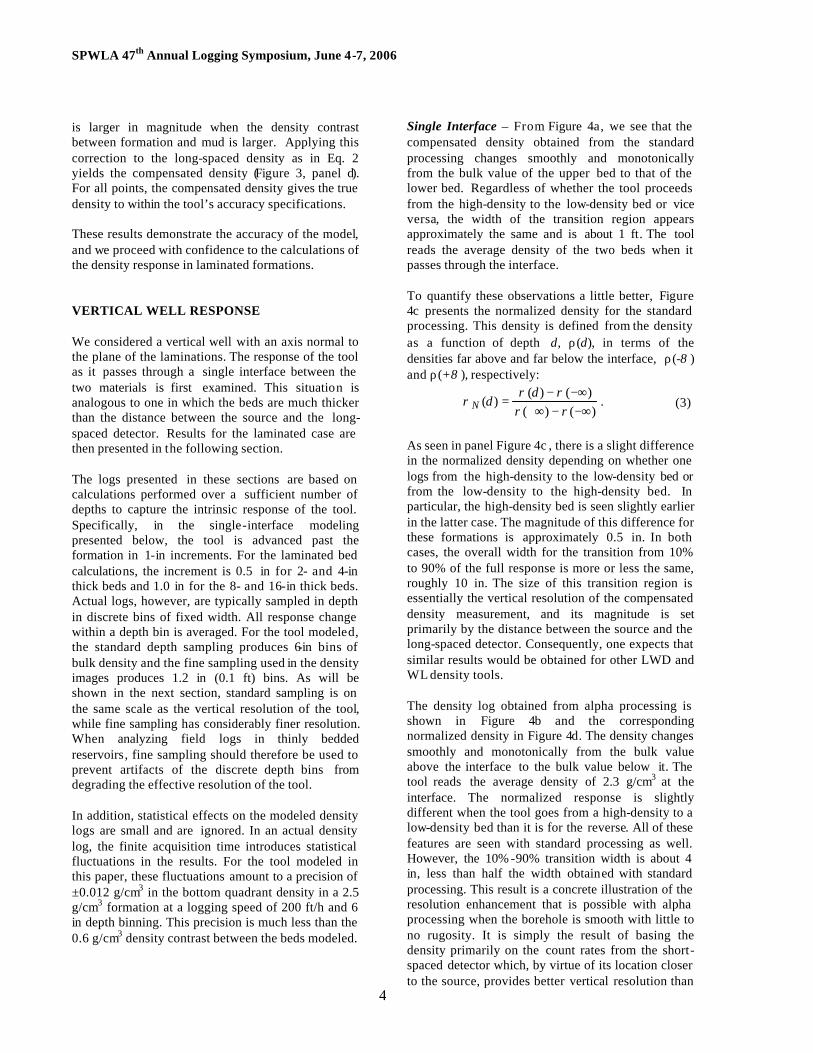
SPWLA 47th Annual Logging Symposium, June 4-7, 2006
4
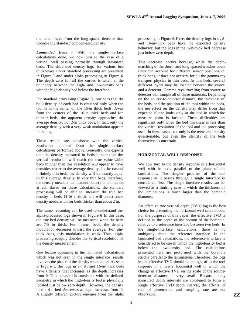
is larger in magnitude when the density contrast between formation and mud is larger. Applying this correction to the long-spaced density as in Eq. 2 yields the compensated density (Figure 3, panel d). For all points, the compensated density gives the true density to within the tool’s accuracy specifications. These results demonstrate the accuracy of the model, and we proceed with confidence to the calculations of the density response in laminated formations. VERTICAL WELL RESPONSE We considered a vertical well with an axis normal to the plane of the laminations. The response of the tool as it passes through a single interface between the two materials is first examined. This situation is analogous to one in which the beds are much thicker than the distance between the source and the long-spaced detector. Results for the laminated case are then presented in the following section. The logs presented in these sections are based on calculations performed over a sufficient number of depths to capture the intrinsic response of the tool. Specifically, in the single-interface modeling presented below, the tool is advanced past the formation in 1-in increments. For the laminated bed calculations, the increment is 0.5 in for 2- and 4-in thick beds and 1.0 in for the 8- and 16-in thick beds. Actual logs, however, are typically sampled in depth in discrete bins of fixed width. All response change within a depth bin is averaged. For the tool modeled, the standard depth sampling produces 6-in bins of bulk density and the fine sampling used in the density images produces 1.2 in (0.1 ft) bins. As will be shown in the next section, standard sampling is on the same scale as the vertical resolution of the tool, while fine sampling has considerably finer resolution. When analyzing field logs in thinly bedded reservoirs, fine sampling should therefore be used to prevent artifacts of the discrete depth bins from degrading the effective resolution of the tool. In addition, statistical effects on the modeled density logs are small and are ignored. In an actual density log, the finite acquisition time introduces statistical fluctuations in the results. For the tool modeled in this paper, these fluctuations amount to a precision of ±0.012 g/cm3 in the bottom quadrant density in a 2.5 g/cm3 formation at a logging speed of 200 ft/h and 6 in depth binning. This precision is much less than the 0.6 g/cm3 density contrast between the beds modeled.
Single Interface – From Figure 4a, we see that the compensated density obtained from the standard processing changes smoothly and monotonically from the bulk value of the upper bed to that of the lower bed. Regardless of whether the tool proceeds from the high-density to the low-density bed or vice versa, the width of the transition region appears approximately the same and is about 1 ft. The tool reads the average density of the two beds when it passes through the interface. To quantify these observations a little better, Figure 4c presents the normalized density for the standard processing. This density is defined from the density as a function of depth d, ρ(d), in terms of the densities far above and far below the interface, ρ(-8 ) and ρ(+8 ), respectively:
)()()()(
)(−∞−+∞
−∞−=
ρρρρ
ρd
dN . (3)
As seen in panel Figure 4c , there is a slight difference in the normalized density depending on whether one logs from the high-density to the low-density bed or from the low-density to the high-density bed. In particular, the high-density bed is seen slightly earlier in the latter case. The magnitude of this difference for these formations is approximately 0.5 in. In both cases, the overall width for the transition from 10% to 90% of the full response is more or less the same, roughly 10 in. The size of this transition region is essentially the vertical resolution of the compensated density measurement, and its magnitude is set primarily by the distance between the source and the long-spaced detector. Consequently, one expects that similar results would be obtained for other LWD and WL density tools. The density log obtained from alpha processing is shown in Figure 4b and the corresponding normalized density in Figure 4d. The density changes smoothly and monotonically from the bulk value above the interface to the bulk value below it. The tool reads the average density of 2.3 g/cm3 at the interface. The normalized response is slightly different when the tool goes from a high-density to a low-density bed than it is for the reverse. All of these features are seen with standard processing as well. However, the 10% -90% transition width is about 4 in, less than half the width obtained with standard processing. This result is a concrete illustration of the resolution enhancement that is possible with alpha processing when the borehole is smooth with little to no rugosity. It is simply the result of basing the density primarily on the count rates from the short-spaced detector which, by virtue of its location closer to the source, provides better vertical resolution than
SPWLA 47th Annual Logging Symposium, June 4-7, 2006
5
the count rates from the long-spaced detector that underlie the standard compensated density. Laminated Beds – With the single-interface calculations done, we now turn to the case of a vertical well passing normally through laminated beds. The simulated density logs for various bed thicknesses under standard processing are presented in Figure 5 and under alpha processing in Figure 6. The depth zero for all the curves is taken at the boundary between the high- and low-density beds with the high-density bed below the interface. For standard processing (Figure 5), one sees that the bulk density of each bed is obtained only when the tool is in the center of the 16-in thick beds. Away from the centers of the 16-in thick beds and for thinner beds, the apparent density approaches the average density. For 2-in thick beds, in fact, only the average density with a very weak modulation appears in the log. These results are consistent with the vertical resolution obtained from the single-interface calculations performed above. Generally, one expects that the density measured in beds thicker than the vertical resolution will reach the true value while beds thinner than this resolution will appear to have densities closer to the average density. In the case of infinitely thin beds, the density will be exactly equal to this average density. In very thin beds, therefore, the density measurement cannot detect the lamination at all. Based on these calculations, the standard processing will be able to measure the true bed density in beds 14-16 in thick, and will detect some density modulation for beds thicker than about 2 in. The same reasoning can be used to understand the alpha-processed logs shown in Figure 6. In this case, the true bed density will be measured when the beds are 7-8 in thick. For thinner beds, the density modulation decreases toward the average. For 2-in-thick beds, this modulation is weak. Thus, alpha processing roughly doubles the vertical resolution of the density measurement. One feature appearing in the laminated calculations which was not seen in the single interface results involves the phas e of the density modulation. As seen in Figure 5, the logs in 2-, 8-, and 16-in-thick beds have a density that increases as the depth increases from 0. This behavior is consistent with the defined geometry in which the high-density bed is physically located just below zero depth. However, the density in the 4-in bed decreases as depth increases from 0. A slightly different picture emerges from the alpha
processing in Figure 6. Here, the density logs in 4-, 8- and 16-in-thick beds have the expected density behavior, but the logs in the 2-in-thick bed decrease just below zero depth. This decrease occurs because, while the depth-matching of the short- and long-spaced window count rates can account for different sensor positions in thick beds, it does not account for all the gamma ray transport physics in thin beds. In thin beds, several different layers may be located between the source and a detector. Gamma rays traveling from source to detector will sample all of these materials. Depending on the source-to-detector distance, the thickness of the beds, and the position of the tool within the beds, the net effect on the density may differ from that expected if one looks only at the bed in which the measure point is located. These difficulties are significant only when the bed thickness is less than the vertical resolution of the tool and the processing used. In these cases , not only is the measured density questionable, but even the identity of the beds themselves is uncertain. HORIZONTAL WELL RESPONSE We now turn to the density response in a horizontal well with its axis parallel to the plane of the laminations. The simpler problem of the tool response as it passes through a single interface is considered first. The single-interface results can be viewed as a limiting case in which the thickness of the laminations is much larger than the borehole diameter. An effective true vertical depth (TVD) log is the best choice for presenting the horizontal well calculations. For the purposes of this paper, the effective TVD is defined as the depth of the bottom of the borehole relative to a reference interface between two beds. In the single-interface calculations, there is no ambiguity about the reference interface. In the laminated bed calculations, the reference interface is considered to be one in which the high-density bed is below the low-density bed. The calculations presented here are performed with the borehole strictly parallel to the laminations. Therefore , the logs in the effective TVD should be thought of as the tool response in a nearly horizontal well in which the change in effective TVD on the scale of the source-detector distance is very small. Because many measured depth intervals are combined to form a single effective TVD depth interval, the effects of rate of penetration and sampling rate are not observable. ZZ

SPWLA 47th Annual Logging Symposium, June 4-7, 2006
6
When comparing these results to field logs, it is worth noting that TVD is defined relative to the bit depth, and so is measured from the center of the borehole. The effective TVD presented here is therefore shifted half a borehole diameter deeper than the TVD seen on the log. This shift may present a challenge to forward modeling and real-time applications of geosteering software when they attempt to correlate multiple log curves with various depths of investigation and orientations in thinly bedded formations. This subject will need to be considered further in future work. Single Interface – The bottom-quadrant density as a function of the effective TVD from a single interface is shown in Figure 7a. As in vertical wells, the apparent density changes smoothly and monotonically from the bulk density of the upper bed to that of the lower bed as the effective TVD increases. The width of the transition region between these densities is also approximately the same whether the high-density or the low-density bed is above the interface. Unlike the vertical case, the densities measured with the bottom of the borehole at the bed interface have almost attained the bulk value of the lower bed. The apparent density equals the average density of the two beds about 1.5 in above the interface rather than at the interface as was seen in the vertical well (Figure 4). Additional features can be seen in Figure 7b, which plots the scaled density computed by Eq. 3. As in the vertical well, we see only a slight difference in the normalized response depending on whether the tool logs from high-to-low or low-to-high density. However, the 10%-90% width of the transition is approximately 4 in rather than the 10 in observed in a vertical well with standard processing. These observations highlight a fundamental difference between vertical and horizontal density response. In a vertical well, an axial geometric factor, the scale of which is set by the source-to-detector distances , determines the response. In horizontal wells, it is the radial geometrical factor that governs the response. Although also related to the source-to-detector distances, the scale of the radial geometrical factor is much smaller than that of the axial geometric factor. This is the origin of the difference in the widths of the transition region. The radial geometrical factor also determines the depth of investigation. Because the tool senses this distance into the formation, as the tool approaches the lower bed from the upper in a horizontal well, the apparent
density value responds to the lower bed long before the interface is encountered. By the time the borehole crosses the interface into the lower bed, the density measurement is already sensing deeper into the lower bed and the bulk value of the density is nearly obtained. A last comment pertaining to alpha processing: the alpha-processing algorithm adjusts the short-spaced density to match the compensated density on average over several feet of measured depth. In the horizontal-well geometries studied here, this procedure would counteract any advantage of the smaller radial geometric factor of the short-spaced detector, since both short-spaced and compensated densities would be approximately constant in measured depth over the averaging interval. Utilizing the uncorrected short-spaced density would provide a shallower measurement (the 10%-90% transition width in the single-interface geometry is about 2 in), but this procedure would introduce serious errors if any tool standoff or borehole rugosity were present. The authors therefore do not recommend this approach for data obtained in horizontal wells . Laminated Beds – The response of the bottom quadrant density in a horizontal well through laminated formations is summarized in Figure 8 for various bed thicknesses. One sees that the true formation densities are obtained with the tool slightly penetrating beds at least 8 in thick. For thinner beds, the amplitude of the density modulation is reduced towards the average density of the two beds. Even for 2-in thick beds, however, the density modulation is significant in contrast to the behavior seen in vertical wells (Figure 5). The ability to detect thinner beds in horizontal well geometries traces back to the difference in axial and radial geometrical factors discussed above. The radial geometrical factor can also be used to understand the position of the extremal densities in Figure 8. For thick beds (Figure 8c and Figure 8d), the extremal densities occur when the borehole penetrates an inch or two into the bed. As the borehole moves deeper into the bed, the density measurement begins to sense through it into the bed beneath. The result is a density that begins to change toward the density of the deeper bed. As seen in the single-interface calculation, the observed density crosses the average density above the interface between these beds. For beds thinner than the depth of investigation of the measurement (Figure 8a ), the extremal density actually occurs in the preceding bed, again since the measurement effectively probes through the material closest to the borehole. It is clear

SPWLA 47th Annual Logging Symposium, June 4-7, 2006
7
that interpreting density logs in horizontal wells through laminated beds becomes complicated when the bed thickness is smaller than the depth of investigation of the tool. CASE STUDY Figure 9 shows WL logs from two wells overlaid on top of one another using a geosteering correlation tool. Both represent offset wells over a reservoir interval in which several horizontal wells were drilled. The magenta curves come from a 20-degree-angle well. The black curves are from a 40-degree-angle well that was conventionally cored over this entire interval. All tracks show good correlation despite the fact that these wells are more than a mile apart. Both standard and enhanced-vertical-resolution (EVR) density processing was preformed on the wells depicted in Figure 9. This processing is an alternative to the alpha processing discussed in previous sections. It has a similar effect of increasing the effective vertical resolution of the density (Smith, 1990). The enhanced density (EVR RHOB) better shows the high contrast in density values in the multiple laminations in this 125-ft measured depth interval. Note that both the standard density (RHOB) and enhanced RHOB show a greater dynamic range in the 40-degree-angle well, particularly in the thin, higher density laminations. Figure 10 shows the WL-logged interval from the 40-degree-angle well of Figure 9, but this time with density data derived from core measure ments overlaid on the RHOB and enhanced RHOB tracks. The lines connecting the core measurements accentuate the thinly bedded nature of the interval. The standard-processed RHOB log does not capture the full range of densities derived from the core. On the other hand, the enhanced RHOB better matches the core. Figure 11 shows a 3-ft section of core that is representative of the reservoir. In the natural light photo on the left, the lighter colored laminations are tight, silty limestone with low porosity and little or no oil saturation. The darker, oil-stained sections are friable siltstones , indurated siltstones , and argillaceous silstones. The thin-section photos seen in Figure 12 show the two end-member lithologies that define the density contrast observed in the core and enhanced RHOB logs. On the left is the relatively clean, high-porosity siltstone. On the right is an example of the low-porosity, silty limestone that is
typical of the high-density laminations. Bioturbation is evident throughout the reservoir sections. For the most part, however, each lamination can be correlated from well to well for miles. Sinusoidal horizontal wells have proven an effective means of producing this formation economically. In such wells, the wellbore oscillates up and down cutting the laminations multiple times (see the bottom track of Figure 13 and Figure 14). Figure 13 compares the LWD bottom-quadrant density (ROBB) from a horizontal well of this kind (black curves) with the WL density data from the 20-degree-angle offset well (magenta curves). In a similar way, Figure 14 shows the same LWD density data compared to the WL density data from the 40-degree-angle well. In both figures, the LWD density from the horizontal well varies much more strongly than the WL densities and is more consistent with the core data. The only WL density which provides a good match to the LWD ROBB is the enhanced RHOB from the 40-degree-angle well. These observations support the conclusions obtained from the modeling. The logs in the near-vertical, 20-degree-angle well are governed by the relatively large vertical resolution of the tool. The laminations have thicknesses which are about the same size as this resolution. Consequently, the density tends toward the average density of the laminations but still shows some modulation in amplitude. As the angle of borehole moves further away from the vertical, as in the 40-degree-angle well, the depth of investigation begins to play a larger role in the response, and the amplitude of the density modulation increases. The best match to the core data arises from the LWD density log acquired in a horizontal well, in which the response is governed by the shallower depth of investigation that can better resolve the laminations. This better resolution results in a more accurate porosity and improved reservoir characterization. CONCLUSIONS In vertical wells through laminated formations, the axial geometrical factor or, equivalently, the vertical resolution determines the tool response. For the LWD tool studied, 16-in-thick beds can be resolved using standard processing, and 8-in-thick beds can be resolved using alpha processing. For very thin layers, the measured density is the average of the densities of the individual layers. However, in horizontal wells through laminated formations, the radial geometrical factor or, in other words, the depth of investigation ZZ

SPWLA 47th Annual Logging Symposium, June 4-7, 2006
8
governs the response. This radial geometrical factor is much smaller than the axial geometric factor, allowing 8-in-thick beds to be resolved without any special processing. In both horizontal and vertical wells, if the beds are thinner than the scale of the relevant geometrical factor, the measured density represents neither the true bed density nor even the geometrical arrangement of the individual layers. In laminations less than about 2 in. thick, the measured density becomes the geometrical average of the individual lamination densities. These results have several implications for formation evaluation in thinly bedded reservoirs. First, the density measurement in horizontal wells can resolve much thinner beds than in vertical wells. Logs in horizontal wells are therefore more accurate than those in vertical wells in these reservoirs. Second, density measurements in either horizontal or vertical wells through thin bed laminations are not always straightforward to interpret. Various combinations of bed thickness and densities can result in the same log response. Accurate estimation of bed boundaries and densities may therefore be difficult in reservoirs with very thin beds of contrasting densities. Obtaining an accurate estimate of a bed’s thickness from images or other information is crucial in ascertaining how much confidence to place in the measured density. ACKNOWLEDGEMENTS The authors would like to thank Chevron for permission to publish the log data in this paper and B. Reik and A. Badruzzaman of Chevron, H. Yin and Q. Passey of ExxonMobil, and D. Allen of Schlumberger for stimulating discussions. REFERENCES CITED Bertozzi, W., Ellis, D.V., and Wahl, J.S., 1981, “The physical foundation of formation lithology logging with gamma rays,” Geophysics, 46, 1439-1455. Ellis, D., Flaum, C., Marienbach, E., Roulet, C., and Seeman, B., 1985, “Litho-density tool calibration,” SPE paper 12048, Society of Petroleum Engineers Journal (August), 515-520. Ellis, D.V., 1987, Well Logging for Earth Scientists, Elsevier, New York. Ellis, D.V., and Chiaramonte, J.M., 2000, “Interpreting neutron logs in horizontal wells: a forward modeling tutorial,” Petrophysics, 41, 23-32.
Evans, M.L., 1981, “A computer model for calculating gamma -ray pulse-height spectra for logging applications,” LA -UR-81-400, Los Alamos National Laboratory, Los Alamos, New Mexico. Flaum, C., Galford, J.E., and Hastings, S., 1987, “Enhanced vertical resolution processing of dual detector gamma -gamma density logs,” 1987 SPWLA Annual Logging Symposium, Paper M. Girard, S. M., ed., 2005, “MCNP — A general Monte Carlo N-particle transport code, version 5,” LA-UR-03-1987, Los Alamos National Laboratory, Los Alamos, New Mexico. Smith, M.P., 1990, “Enhanced vertical resolution processing of dual-spaced neutron and density tools using standard shop calibration and borehole compensation procedures,” SPWLA Annual Logging Symposium, Paper SS. Passey, Q.R., Yin, H., Rendeiro, C.M., Fitz, D.E., 2005, “Overview of high-angle and horizontal well formation evaluation: issues, learnings, and future directions,” 2005 SPWLA Annual Logging Symposium, Paper A. ABOUT THE AUTHORS R. J. Radtke is a senior tool physicist in Sugar Land, Texas. He is involved in the design, characterization, and algorithm development for nuclear LWD and WL tools. Before joining Schlumberger in 1999, he had post-doctoral appointments at Harvard University and the University of Maryland after graduating from The University of Chicago in 1994 with a PhD in physics. Mike Evans joined Schlumberger in 1981 in Houston, where he worked on several wireline nuclear logging tools. In 1986, he joined the LWD project in Sugar Land, Texas, where he was involved in the design and interpretation of nuclear tools. He is currently working with a nuclear group. John Rasmus is an advisor in the LWD interpretation field and client support organization based in Sugar Land, Texas. He has held various interpretation development positions, developing new and innovative interpretation techniques for secondary porosity in carbonates, geosteering of horizontal wells, and geopressure quantifications. John earned a BS degree in mechanical engineering from Iowa State University and an MS degree in petroleum engineering from the University of

SPWLA 47th Annual Logging Symposium, June 4-7, 2006
9
Houston and is a registered professional engineer in Texas. Darwin V. Ellis is a scientific advisor at Schlumberger-Doll Research Center. He began his career with Schlumberger after obtaining a PhD in physics and space science from Rice University. He has worked in many capacities in Schlumberger in Houston, Paris (where he engineered a density logging tool), and Ridgefield in nearly four decades of well logging research and engineering. Ten years ago he was a recipient of the SPWLA Distinguished Technical Achievement Award. He is the author of more than 100 internal and external reports and has been granted 7 patents. Currently he is working on a second edition of his textbook, Well Logging for Earth Scientists, with co-author Julian Singer. Joseph M. Chiaramonte joined Schlumberger-Doll Research Center in 1982 and is currently a senior research scientist in the nuclear program. His primary interest has been in developing and implementing improved methods for codes used to model nuclear well logging devices. Mr. Chiaramonte is the author or co-author of over 40 internal company reports and 12 external articles, and is a member of the American Nuclear Society. Mr. Chiaramonte received an MA in applied mathematics from Western Connecticut State University in 1982. Charles R. Case is currently a private consultant for the oil and gas industry. He was a senior research scientist at Schlumberger-Doll Research Center until 2004. He received his BA degree in physics from Northeastern University, Boston, Massachusetts , and his MS degree in physics from Trinity College, Hartford, Connecticut, graduating from both universities with honors. He has been a part of the nuclear industry for over 30 years, starting at Bettis Atomic Power Laboratory in Pittsburgh, Pennsylvania, where he worked on the successful Light Water Breeder Reactor project before joining Schlumberger in 1979, where he specialized in the theoretical design, analysis and interpretation of nuclear logging devices. He jointly holds two U.S. patents related to logging. Ed Stockhausen is a senior research scientist for Chevron Energy Technology Company and is based in Houston, Texas. Ed graduated from the University of Florida with an MS degree in geology in 1981. Over the next 16 years, he held various exploration and production geology positions for Chevron in New Orleans, focusing on Gu lf of Mexico field development. For the past eight years, Ed has been responsible for leading the development and
deployment of geosteering technology for Chevron worldwide. Ed has presented papers and posters at various technical conferences, forums, and society meetings on horizontal well case histories, geosteering methods, the design of flexible well paths, and the pitfalls of directional surveying practices.
Fig. 1 Schematic comparison of the physical processes occurring during the operation of the density tool and the approach used in the modeling.
Fig. 2 How window count rates from either model or actual logging tool convert into densities.
Calibrate to Al, Mg densities
Depth and resolution matching
Density log
Measured window count rates from formation and
Al, Mg blocks
Modeled MCNP window count rates from formation and
Al, Mg blocks
PE and rib corrections
Pulse Height Spectra
Window Count Rates
Model
MCNP: Photon Current J
Pulse Height P = R • J
GAMRES: Response R
Detector
Tool
Source
PMT
Electronics
ZZ
SPWLA 47th Annual Logging Symposium, June 4-7, 2006
10
1.5 2 2.5 3-0.2
-0.1
0
0.1
0.2SS Density
Den
sity
Err
or (g
/cm
3 )
1.5 2 2.5 3-0.2
-0.1
0
0.1
0.2LS Density
1.5 2 2.5 3-0.2
-0.1
0
0.1
0.2∆ρ
Den
sity
Err
or (g
/cm
3)
Density (g/cm3)1.5 2 2.5 3
-0.2
-0.1
0
0.1
0.2Compensated Density
Density (g/cm3) Fig. 3 Benchmarking results for the model. The tool is fully eccentered in an 8.50-in fresh-water-filled borehole through a homogeneous formation as shown in the inset. In this inset, brown represents the formation; dark gray, the stabilizer; light gray, the collar and chassis; red, the source; green, the detectors; light orange, the collimators; and light blue, the drilling fluid. The tool accuracy of ±0.015 g/cm3 is indicated by the heavy black lines.
Fig. 4 Density response in vertical well as tool logs through single interface as shown in inset. In this inset, brown or marbled gray represents the formation; dark gray, the stabilizer; light gray, the collar and chassis; red, the source; green, the detectors; light orange, the collimators; and light blue, the drilling fluid. The apparent density as a function of depth is shown for standard processing and alpha processing as the tool travels from the low- to the high-density bed (red) and the high- to the low-density bed (blue). Densities normalized to the initial and final values are also shown for standard processing and alpha processing. The widths of the 10% to 90% response are indicated.
Tool accuracy specs
Al Mg
(a) (b)
(c) (d)
2 2.2 2.4 2.6
-12-8-4048
12
Standard Processing
Dep
th (i
n)
Density (g/cm3)
0 0.5 1
-12-8-4048
12
Dep
th (i
n)
Normalized Density
2 2.2 2.4 2.6
-12-8-4048
12
Alpha Processing
Density (g/cm3)
0 0.5 1
-12-8-4048
12
Normalized Density
2.6 g/cm3
2.6 g/cm3
2.0 g/cm3
10 in
4 in
0
(d)
(b) (a)
(c)
0

SPWLA 47th Annual Logging Symposium, June 4-7, 2006
11
2.0 2.6
-18
-12
-6
0
6
12
18
2.0 in. BedsD
epth
(in.
)
2.0 2.6
-18
-12
-6
0
6
12
18
4.0 in. Beds
2.0 2.6
-18
-12
-6
0
6
12
18
8.0 in. Beds
2.0 2.6
-18
-12
-6
0
6
12
18
16.0 in. Beds
2.0 2.6
-18
-12
-6
0
6
12
18
2.0 in. Beds
Dep
th (i
n.)
2.0 2.6
-18
-12
-6
0
6
12
18
4.0 in. Beds
2.0 2.6
-18
-12
-6
0
6
12
18
8.0 in. Beds
2.0 2.6
-18
-12
-6
0
6
12
18
16.0 in. Beds
Fig. 5 Density response in a vertical well as the tool logs through a set of laminated beds of various thicknesses obtained from standard processing. The inset shows the approximate geometry for the case of 4-in-thick beds. In this inset, brown or marbled gray represents the formation; dark gray, the stabilizer; light gray, the collar and chassis; red, the source; green, the detectors; light orange, the collimators; and light blue, the drilling fluid.
Fig. 6 Density response in vertical well as tool logs through laminated beds of various thicknesses obtained from alpha processing. The inset shows the approximate geometry for the case of 4-in-thick beds. In this inset, brown or marbled gray represents the formation; dark gray, the stabilizer; light gray, the collar and chassis; red, the source; green, the detectors; light orange, the collimators; and light blue, the drilling fluid.
2.6 g/cm3
2.0 g/cm3
0
Density (g/cm3)
Dep
th (
in)
2.6 g/cm3
2.0 g/cm3
0
Density (g/cm3)
Dep
th (
in)
Vertical Well, Standard Processing
Vertical Well, Alpha Processing
ZZ

SPWLA 47th Annual Logging Symposium, June 4-7, 2006
12
2.0 2.6
-18
-12
-6
0
6
12
18
2.0 in. Beds
Dep
th (i
n.)
2.0 2.6
-18
-12
-6
0
6
12
18
4.0 in. Beds
2.0 2.6
-18
-12
-6
0
6
12
18
8.0 in. Beds
2.0 2.6
-18
-12
-6
0
6
12
18
10.0 in. Beds
Fig. 7 Density response in horizontal well as tool moves through single interface.
Fig. 8 Density response in horizontal well as tool moves through laminated beds of various thicknesses. The inset shows the approximate geometry for the case of 4-in-thick beds. In this inset, brown or marbled gray represents the formation; dark gray, the stabilizer; light gray, the collar and chassis; red, the source; green, the detectors; light orange, the collimators; and light blue, the drilling fluid. The depth zero is shown in the inset and corresponds to the borehole tangent to the interface between the two beds with the higher density bed below the tool.
2.6 g/cm3
2.0 g/cm3
2.6 g/cm3
2 2.2 2.4 2.6
-6
-4
-2
0
2
4Effe
ctiv
e T
VD
(in.
)
Bottom-Quadrant Density (g/cm3)
0 0.5 1
-6
-4
-2
0
2
4Effe
ctiv
e T
VD
(in
.)
Normalized Density
0
0
4 in
(a)
(b)
Effe
ctiv
e T
VD
(in
) E
ffect
ive
TV
D (
in)
2.6 g/cm3
2.0 g/cm3
0
Density (g/cm3)
Dep
th (
in)
Horizontal Well

SPWLA 47th Annual Logging Symposium, June 4-7, 2006
13
Fig. 9 Wireline logs taken from 20- (magenta curves) and 40-deg-angle (black curves) wells over the same stratigraphic reservoir interval. Gamma ray is in Track 1, resistivity in Track 2, standard-processed density in Track 3, and enhanced-vertical-resolution-processed density in Track 4. The effect of the higher well inclination is to enhance the apparent resolution of the measurements. Depth increment is 10 ft. TVD per division. Fig. 10 Wireline log taken through a cored interval in a 40-deg-angle well. Gamma ray is in Track 1, resistivity in Track 2, measured core and standard-processed density in Track 3, and measured core and enhanced-vertical-resolution-processed density in Track 4. Compared to the 20-deg-angle well data in Figure 9, the combination of higher well inclination with enhanced resolution processing results in a better match to the core density. Depth increment is 10 ft. TVD per division.
G a m m a R a y 2 0o w e l l
G a m m a R a y 4 0o w e l l
D e e p Ind R e s 20 o well
D e e p I n d R e s 4 0 o w e l l
M e d I n d R e s 40 o well W L R H O B - 4 0 o w e l l
W L R H O B – 2 0 o w e l l W L E V R R H O B – 2 0 o w e l l
W L E V R R H O B – 4 0 o w e l l
G a m m a R a y 2 0o w e l l
G a m m a R a y 4 0o w e l l
D e e p Ind R e s 20 o well
D e e p I n d R e s 4 0 o w e l l
M e d I n d R e s 40 o well W L R H O B - 4 0 o w e l l
W L R H O B – 2 0 o w e l l W L E V R R H O B – 2 0 o w e l l
W L E V R R H O B – 4 0 o w e l l
G a m m a R a y 4 0 o w e l l
D e e p I n d R e s 4 0o well
M e d I n d R e s 40 o well W L R H O B - 40 o wel l
C o r e D e n s i t y ( t a k e n i n 4 0 o well )
W L E V R R H O B – 40 o wel l
C o r e D e n s i t y ( t a k e n i n 4 0 o well)C o r e G a m m a R a y
G a m m a R a y 4 0 o w e l l
D e e p I n d R e s 4 0o well
M e d I n d R e s 40 o well W L R H O B - 40 o wel l
C o r e D e n s i t y ( t a k e n i n 4 0 o well )
W L E V R R H O B – 40 o wel l
C o r e D e n s i t y ( t a k e n i n 4 0 o well)C o r e G a m m a R a y
ZZ

SPWLA 47th Annual Logging Symposium, June 4-7, 2006
14
Fig. 11 Core photograph taken from a representative interval shown in Figure. 9. The dark areas represent porous siltstones with high oil saturations, while the lighter areas represent calcite-cemented, low-porosity siltstones with little to no oil saturation. Many of these beds are less than 1 ft thick. The location of the core plugs has been chosen such that the plugs represent either the porous or non-porous lithologies.
Fig. 12 Thin sections taken from the core plugs showing the porous siltstones on the left , evidenced by the light blue epoxy filling the pore space. Calcite-cemented, low-porosity zones are illustrated on the right, with the pink -colored calcite filling the pore space.
X598
X601
X600
X599

SPWLA 47th Annual Logging Symposium, June 4-7, 2006
15
Fig. 13 Comparison of WL data from the 20-deg-angle well (magenta curves) to LWD density data from a horizontal well (black curves). The density scale is 1.95 to 2.95 g/cm3, and the depth increment is 100 ft TVD per division. The image track at the top of the figure contains the measured LWD density image. The next two tracks contain the density images derived from the WL -measured densities in the 20-deg-angle well convolved with the trajectory and the LWD-derived stratigraphy shown in the bottommost track . The apparent density resolution increases with well angle.
Gam
ma
Ray
Hor
wel
l
A34
H R
esH
or
wel
l
P34
H R
esH
or
wel
l
LW
D R
HB
B -
Hor
wel
l
WL
RH
OB
-20o
wel
l
LW
D R
OB
B –
Hor
wel
l
WL
EV
R R
HO
B -2
0ow
ell
Gam
ma
Ray
20
o
wel
l
Dee
p In
dR
es
20o
wel
l
Gam
ma
Ray
Hor
wel
l
A34
H R
esH
or
wel
l
P34
H R
esH
or
wel
l
LW
D R
HB
B -
Hor
wel
l
WL
RH
OB
-20o
wel
l
LW
D R
OB
B –
Hor
wel
l
WL
EV
R R
HO
B -2
0ow
ell
Gam
ma
Ray
20
o
wel
l
Dee
p In
dR
es
20o
wel
l
WL RHOB20o well
WL EVR RHOB 2 0o well
LWD density Image Hor well
WL RHOB20o well
WL EVR RHOB 2 0o well
LWD density Image Hor well
Tra
ject
ory
and
stru
ctur
al c
ross
-
sect
ion
ZZ

SPWLA 47th Annual Logging Symposium, June 4-7, 2006
16
Fig. 14 Comparison of WL data from the 40-deg-angle well (magenta curves) to LWD density from a horizontal well data (black curves). The density scale is 1.95 to 2.95 g/cm3, and the depth increment is 100 ft TVD per division. The image track at the top of the figure contains the measured LWD density image. The next two tracks contain the density images derived from the WL-measured densities in the 40-deg-angle well convolved with the trajectory and the LWD-derived stratigraphy shown in the bottommost track . The measured LWD density more accurately represents the reservoir properties.
Tra
ject
ory
and
stru
ctur
al c
ross
-
sect
ion
WL RHOB40o well
WL EVR RHOB 40o well
LWD density Image Hor well
WL RHOB40o well
WL EVR RHOB 40o well
LWD density Image Hor well
Gam
ma
Ray
Hor
wel
l
A34
H R
esH
or
wel
l
P34
H R
esH
or
wel
l
LW
D R
HB
B -
Hor
wel
l
WL
RH
OB
-40o
wel
l
LW
D R
OB
B –
Hor
wel
l
WL
EV
R R
HO
B -4
0ow
ell
Gam
ma
Ray
40
o
wel
l
Dee
p In
dR
es
40o
wel
l
Gam
ma
Ray
Hor
wel
l
A34
H R
esH
or
wel
l
P34
H R
esH
or
wel
l
LW
D R
HB
B -
Hor
wel
l
WL
RH
OB
-40o
wel
l
LW
D R
OB
B –
Hor
wel
l
WL
EV
R R
HO
B -4
0ow
ell
Gam
ma
Ray
40
o
wel
l
Dee
p In
dR
es
40o
wel
l


![Laminations and Packages from NiFe-Alloys [1] · Laminations and Packages from NiFe-Alloys [1] Laminations and EK Core Packages from MUMETALL®, VACOPERM® und PERMENORM® Introduction](https://img.pdfslide.net/doc/110x75/6049a9d9ea48000c1e32a8fb/laminations-and-packages-from-nife-alloys-1-laminations-and-packages-from-nife-alloys.jpg)


![7RSORWQD ]Då LWD ]XQDQMLK VWHQ](https://img.pdfslide.net/doc/110x75/61708e7db30ceb5beb0af62e/7rsorwqd-d-lwd-xqdqmlk-vwhq.jpg)