M O T I A

Modelling Tools for Interdependence Assessment in ICT Systems

(JLS/2009/CIPS/AG/C1-016)

A C T I V I T Y II A C T I V I T Y II

Relationship among ICT networks and systemsRelationship among ICT networks and systems

Version 1.0

Leading organization for this Activity: CNR-IIT.

With the support of the Prevention, Preparedness and Consequence Management of Terrorism and other Security-

related Risks Programme' European Commission - Directorate-General Justice, Freedom and Security'

This project has been funded with support from the European Commission. This publication reflects the

views only of the author, and the Commission cannot be held responsible for any use which may be made of the information contained therein

Dissemination Level PU Public

Editor(s) CNR-IIT: Enrico Gregori

ENEA: Gregorio D'Agostino

Author(s) (CNR-IIT) Enrico Gregori ... (Caspur) Emiliano Casalicchio, ... (ENEA) Gregorio D'Agostino (MIX-IT srl)... (Namex) ... (Regione Toscana) ... (Telcom Italia) ... (TOP-IX) ...

Contributor(s) … (if any)

Activity 1 Extension idea & methodologies to EU networks Remarks

Changes Authors and added contributes Date Enrico Gregori 18/03/2011

Review

Approval date Remarks

Index Index .................................................................................................................................................... 4  List of Figures...................................................................................................................................... 5  1.   Introduction................................................................................................................................... 6  

1.1.   Data collection ....................................................................................................................... 6  1.2.   Data analysis .......................................................................................................................... 7  

2.   Topological structure and system elements .................................................................................. 9  2.1.   Physical and Data Link layers ............................................................................................... 9  2.1.1.   Example of optical backbone............................................................................................ 10  2.2.   IP layer................................................................................................................................. 14  

2.2.1.   Measurement tools........................................................................................................ 14  2.2.2.   Internet AS-level topology model ................................................................................ 16  2.2.3.   Validation of data ......................................................................................................... 18  2.2.4.   Analysis of Internet dataset .......................................................................................... 20  

3.   Coupling Analysis ...................................................................................................................... 22  3.1.   Enriching the topology with tags ......................................................................................... 22  

3.1.1.   IXP tag .......................................................................................................................... 22  3.1.2.   Geographical tag........................................................................................................... 25  3.1.3.   Business tag .................................................................................................................. 26  

3.2.   Linking multiple layers........................................................................................................ 26  Bibliography ...................................................................................................................................... 28  

List of Figures Figure 1 - National optical backboneTelecom Italia Phoenix structure ............................................ 11  Figure 2 - Simplified description of the mechanism of Fast Restoration in case of a single network

failure. ........................................................................................................................................ 13  Figure 3 - Average neighbor degree vs. degree ................................................................................ 21  Figure 4 - Average clustering coefficient vs. degree. ........................................................................ 21  Figure 5 - Degree CCDF.................................................................................................................... 22  Figure 6 –Presence of participants..................................................................................................... 24  Figure 7 - Traceroutes and BGP contributions to connections on IXPs of Merge dataset. .............. 25  

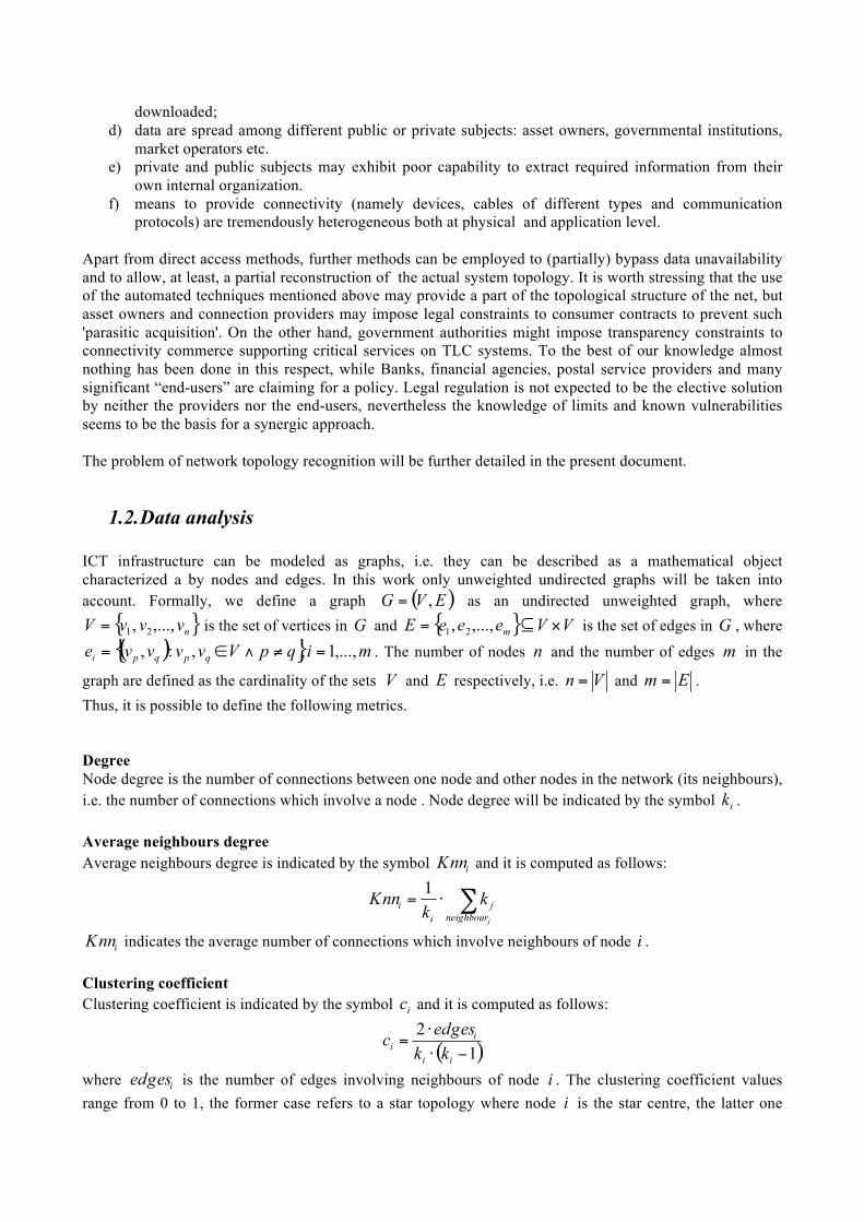
1. Introduction The present document aims at defining the support that topological analysis of complex networks (representing Critical Infrastructures at the highest level of abstraction) might provide to provide insights and to identify basic interdependency mechanisms and effects. The Internet infrastructure (or any other ICT infrastructure) can be initially regarded (and modeled) as a mathematical object, a graph, consisting of different elements such as nodes and arcs (or links) which are functional elements connecting the nodes. Despite its simplicity (the graph metaphor does not account for the complexities related to the structure of nodes, the type of information that flows in its links etc.), the graph may representation a useful mathematical object since it is able to store and resume a number of relevant properties of the network. The former can be unveiled by evaluating topological graph's properties by means of mathematical tools. The main purpose of the present chapter is to provide a basic discussion on the topological approach to the internet (or other ICT net) analysis. The results of this preliminary analysis, can be valuable to understand basic features of the very complex infrastructures one has to deal with. Graph analysis is an old branch of mathematics. However, much work has been devoted in this domain during the last years as the methodological approach (the reduction of complex systems to graphs) has been used to study a large variety of complex systems: genomics, biological objects, social aggregation of humans (crowds) etc. Technological and virtual objects (the Internet, the WWW etc.) have been studied by first reducing their structure and complexity into a simple graph. This approach has been also adopted to understand complex phenomena acting in these systems, such as growth mechanisms (often complex systems grow with no external supervision; the growth mechanism is thus a critical information able to unveil relevant properties of the system under study), synchronization etc. Several seminal works have been published in recent years on these topics [1][2][3]: the reader is referred to these work for a deeper and mathematically rigorous treatment. Basic concepts have been reported here for self-consistency purposes.

1.1. Data collection The first problem to be faced when dealing with the analysis of Critical Infrastructures in general and especially the Internet is data collection. Correctness and completeness of data represent prerequisites to perform any reliable analysis, The straightest (and most effective) means to achieve reliable data is represented by the direct provision from the asset owners or asset managers, that is collecting them from the private or public entities having a direct commitment in the operation of the infrastructures. Apart from direct acquisition, other methods can be used to (partially) bypass data unavailability and to allow, at least, a partial reconstruction of the actual system topology. Data are often available in the form of GIS (Geographic Information System) databases that can be used in appropriate viewer allowing immediate data contextualization and their merging in wider complex scenarios. Direct acquisition, however, usually encounters several drawbacks that have been identified and, ipso facto, undermine the accessibility of data to be used in the analysis. Among them, it is worth quoting the following:

a) privacy laws may forbid or limit data release; b) when owned by private companies, data access can be restricted for both security and marketing

policies; c) data are stored by the CI owners in complex formats, rich of details, such as GIS and similar format

on proprietary databases which, although being accessible, cannot be used as a whole and

downloaded; d) data are spread among different public or private subjects: asset owners, governmental institutions,

market operators etc. e) private and public subjects may exhibit poor capability to extract required information from their

own internal organization. f) means to provide connectivity (namely devices, cables of different types and communication

protocols) are tremendously heterogeneous both at physical and application level. Apart from direct access methods, further methods can be employed to (partially) bypass data unavailability and to allow, at least, a partial reconstruction of the actual system topology. It is worth stressing that the use of the automated techniques mentioned above may provide a part of the topological structure of the net, but asset owners and connection providers may impose legal constraints to consumer contracts to prevent such 'parasitic acquisition'. On the other hand, government authorities might impose transparency constraints to connectivity commerce supporting critical services on TLC systems. To the best of our knowledge almost nothing has been done in this respect, while Banks, financial agencies, postal service providers and many significant “end-users” are claiming for a policy. Legal regulation is not expected to be the elective solution by neither the providers nor the end-users, nevertheless the knowledge of limits and known vulnerabilities seems to be the basis for a synergic approach. The problem of network topology recognition will be further detailed in the present document.

1.2. Data analysis ICT infrastructure can be modeled as graphs, i.e. they can be described as a mathematical object characterized a by nodes and edges. In this work only unweighted undirected graphs will be taken into account. Formally, we define a graph as an undirected unweighted graph, where

is the set of vertices in and is the set of edges in , where

. The number of nodes and the number of edges in the

graph are defined as the cardinality of the sets and respectively, i.e. and . Thus, it is possible to define the following metrics. Degree Node degree is the number of connections between one node and other nodes in the network (its neighbours), i.e. the number of connections which involve a node . Node degree will be indicated by the symbol . Average neighbours degree Average neighbours degree is indicated by the symbol and it is computed as follows:

indicates the average number of connections which involve neighbours of node . Clustering coefficient Clustering coefficient is indicated by the symbol and it is computed as follows:

where is the number of edges involving neighbours of node . The clustering coefficient values range from 0 to 1, the former case refers to a star topology where node is the star centre, the latter one

indicates a full mesh between neighbours. provides a measure of the local connectivity structure of the network. Betweenness centrality Node betweenness centrality, is the number of shortest paths that pass through the node . gives a measure of the amount of traffic that goes through it [4], if routing is guided by shortest-path-based algorithm. Nevertheless, since routing is not necessarily guided by shortest-path policies, betweenness centrality could completely results uncorrelated to load of each node. Defined metrics correspond to local properties: in order to have a large-scale view of topologies represented by graphs it is necessary to shift attention to statistical measures which can take into account global behaviour of these quantities. here are defined some of these statistical metrics and some other new ones. Components A connected component of an undirected graph G is a subgraph H in which any two vertices are connected to each other by paths, and to which no more vertices or edges (from the larger graph) can be added while preserving its connectivity. That is, it is a maximal connected subgraph. A graph that is itself connected has exactly one connected component, consisting of the whole graph. The number of connected components is an important topological invariant of a graph. In topological graph theory it can be interpreted as the zeroth Betti number of the graph [7]. In algebraic graph theory it equals the multiplicity of 0 as an eigenvalue of the Laplacian matrix of the graph. It is also the index of the first nonzero coefficient of the chromatic polynomial of a graph [8]. Complementary cumulative distribution function of degree, , represents the probability one node has a degree greater than k. If degree distribution follows a power law, i.e. a function which has the form , the network is named scale-free. In 2001, Internet AS level graph inferred by [4] had a

. Shortest path and diameter Shortest path length, , measures the number of edges forming the shortest path (i.e. minimum number of

steps required) from to . Average shortest path length, , is the average value considering all node

couples. Diameter, is the maximum value of , considering all possible pairs , . Small world property A network is called a small-world network if most nodes can be reached from every other with a small number of hops. This type of networks will show:

• probably, an high number of cliques, i.e. an high value of clustering coefficient (this features is not necessary since a star topology graph also presents a small average shortest path value);

• a small average shortest path; • probably, there are many hub nodes (high degree nodes).

The average shortest path of Internet AS level graph is the order of magnitude of 1, it will assume values around 3. Shortest paths probability distribution will be similar to a Gaussian function. Neighbor connectivity Assortativity is a graph property which indicates the degree of correlation between nodes: neighbour connectivity is able to capture that. Neighbour connectivity is the average degree of neighbours of nodes with degree and it is indicated with . Networks can be assortative or disassortative (or neither): the former case occurs if the neighbour connectivity function is increasing, i.e. nodes with low degree tend to connect to nodes with low degree

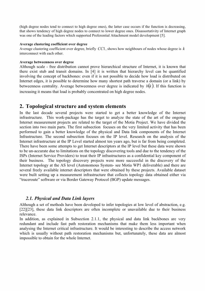
(high degree nodes tend to connect to high degree ones), the latter case occurs if the function is decreasing, that shows tendency of high degree nodes to connect to lower degree ones. Disassortativity of Internet graph was one of the leading factors which supported Preferential Attachment model development [5]. Average clustering coefficient over degree Average clustering coefficient over degree, briefly , shows how neighbours of nodes whose degree is interconnect with each other. Average betweenness over degree Although scale - free distribution cannot prove hierarchical structure of Internet, it is known that there exist stub and transit domains. In [4] it is written that hierarchy level can be quantified involving the concept of backbones: even if it is not possible to decide how load is distributed on Internet edges, it is possible to determine how many shortest path traverse a domain (or a link) by betweenness centrality. Average betweenness over degree is indicated by . If this function is increasing it means that load is probably concentrated on high degree nodes.

2. Topological structure and system elements In the last decade several projects were started to get a better knowledge of the Internet infrastructure. This work-package has the target to analyze the state of the art of the ongoing Internet measurement projects are related to the target of the Motia Project. We have divided the section into two main parts. The first subsection focuses on the very limited activity that has been performed to gain a better knowledge of the physical and Data link components of the Internet Infrastructure. The second subsection focuses on the IP level. Research on the analysis of the Internet infrastructure at the IP Level started almost ten years ago, but is far from being completed. There have been some attempts to get Internet descriptors at the IP level but these data were shown to be un-accurate due to limitations on the topology discovering tools and due to the tendency of the ISPs (Internet Service Providers) to treat their IP infrastructures as a confidential key component of their business. The topology discovery projects were more successful in the discovery of the Internet topology at the AS level (Autonomous System- see Motia WP1 deliverable) and there are several freely available internet descriptors that were obtained by these projects. Available dataset were built setting up a measurement infrastructure that collects topology data obtained either via “traceroute” software or via Border Gateway Protocol (BGP) update messages.

2.1. Physical and Data Link layers Although a set of methods have been developed to infer topologies at low level of abstraction, e.g. [22][23], these data link descriptors are often incomplete or unavailable due to their business relevance. In addition, as explained in Subsection 2.1.1, the physical and data link backbones are very redundant and include fast path restoration mechanisms that make them less important when analysing the Internet critical infrastructure. It would be interesting to describe the access network which is usually without path restoration mechanisms but, unfortunately, these data are almost impossible to obtain for the whole Internet.

2.1.1. Example of optical backbone

The two main components of the Arianna network are the Phoenix for the long haul transmission systems based on technology of wavelength division multiplexing (DWDM), already widely used in the network of Telecom Italia since 1999, and the new equipment to cross connection-Marconi Communications MSH2k supply high-capacity listed below by the acronym ODXC (Optical Digital Cross Connect). DWDM transport systems provide high-speed flows of up to forty 10-Gb / s and the ODXC, thanks to the processing units and high-performance control crews, as well as ensuring the SDH standard features already present. Arianna network permits, together with a suitable chain management system, the implementation of mechanisms for fast recovery of traffic (Fast Restoration) in case of failure. Architecture and Main Features - Phoenix, based on the ODXC equipment, will be in the near future the main national broadcasting platform for most applications of Telecom Italia. It is a meshed network and the network nodes, each equipped with one or more ODXC, are interconnected by optical fiber or DWDM systems. The connections between the various ODXC, conveyed on DWDM systems or directly to optical fibers, are 2.5 Gbps or 10 Gbps links to the devices while users can have speeds from 155 Mbps 10 Gbps with a granularity of 155 Mbps. Structure and interconnection with other networks - The structure of Phoenix updated in October 2004 is shown in Figure 1. As can be seen from the drawing the network has a meshed structure and all nodes, except for some specific cases, have at least three outgoing degree, that have at least three ways out thus ensuring protection to at least double simultaneous failure of the carrier. We will see later that this network, if properly sized, is able to withstand on average a much higher failure transmission network contemporaries. Each node is equipped with one or more ODXC based on the amount of traffic that must be transported. The typical connections to other networks are shown in Figure 2. The ODXC is, like all cross connect, a symmetric system in the sense that unlike ADM does not have a set of dedicated ports for the transmission line and for clients, and each port can be used either to connect two or ODXC to connect customer equipments.

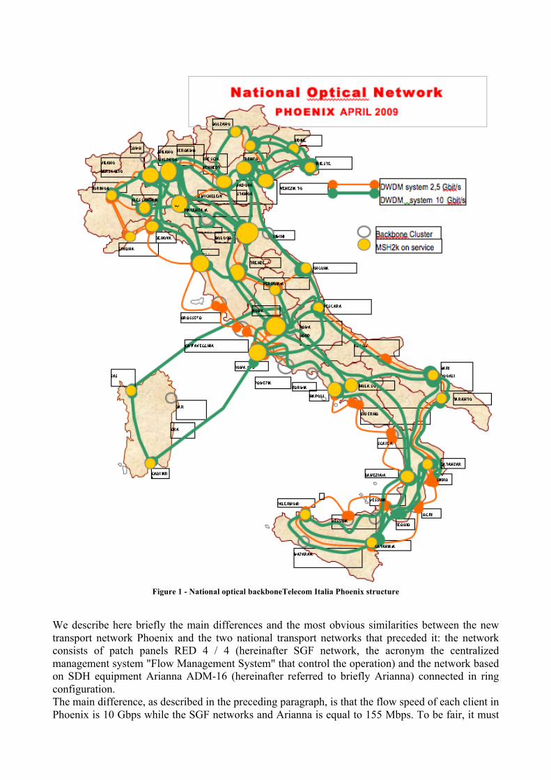
Figure 1 - National optical backboneTelecom Italia Phoenix structure

We describe here briefly the main differences and the most obvious similarities between the new transport network Phoenix and the two national transport networks that preceded it: the network consists of patch panels RED 4 / 4 (hereinafter SGF network, the acronym the centralized management system "Flow Management System" that control the operation) and the network based on SDH equipment Arianna ADM-16 (hereinafter referred to briefly Arianna) connected in ring configuration. The main difference, as described in the preceding paragraph, is that the flow speed of each client in Phoenix is 10 Gbps while the SGF networks and Arianna is equal to 155 Mbps. To be fair, it must

be said that the network Arianna would be able to deliver higher speed flows, such as 622 Mbps or 2.5 Gbps, but the ring architecture and the fact that the product on which it is based is an ADM-16 (able to achieve only one ring at 2.5 Gbps). In addition, the new network will be able to carry, once available on the matrix OTH MSH2k equipment, STM-16 and STM-64 signals in transparent mode, i.e. without changing in any way the payload. As for survival to faults, Phoenix uses a mechanism called Fast Restoration, which can be easily understood by imagining a rationale for the mechanisms of automatic protection available on Arianna, and, in particular, SNCP protection type (Sub Network Connection Protection) is available on the connecting ring, and the mechanism of restoration of the SGF network. Before going into details of the operation Fast Restoration, it is useful to briefly describe the mechanisms for automatic protection and restoration. Let's see the security level in case of the failure that occurs between two nodes of the network: traffic is switched to a backup path previously computed between that pair of nodes. The protection level can be either a dedicated section, also called 1+1: this scheme provides a full replication of the data flow of secure connection to two connections, one operating and one spare, with double occupancy of bandwidth. In case of failure, it is sufficient that only the receiving node switches its reception on the channel reserve, a task that can be done in a very short time. The protection mechanism at the level of path is implemented only by the initial and terminal nodes of a path and requires the identification of a whole section of the reserve. Even in this new scenario we can envisage a dedicated 1 +1 protection where the paths of the operation and reserves are calculated simultaneously and the entire flow of transmission is duplicated on both routes, leaving the receiver in charge of selecting the best flow characteristics; performance is excellent in terms of recovery time, but low in terms of efficient use of available bandwidth in the network. The classical mechanisms of restoration (to distinguish them from those of Fast Restoration) can also be divided into restoration and restoration at the level path. In comparison to similar mechanisms of protection, the main difference is that the automatic transmission resources dedicated to the route of protection are not pre-allocated and shared by a variety of principal circuits. It is clear that the absence of a pre-allocation of transmission resources to provide protection at the time of failure and the activation of the process that compute the new route, dramatically reduces the effectiveness of protection and increases the downtime. In addition, the sharing of protection resources requires a process of planning for themselves far more complex than in the case of automatic protection. In very general terms we can say that the Arianna network, based on the mechanisms of protection and automatic MS-Spring SNCP, reduces the protection operating time (typically less than 50 ms, independent of the number of circuits to be protected) to the detriment efficiency of resource use, while the SGF network, based on the mechanism of restoration without pre-allocation, increases the efficient use of resources at the expense of response time (typically in the order of minutes, and strongly dependent on the number of circuits to be protected). The Fast Restoration provides a constant product of the operation time and efficiency, managing simultaneously to contain the response time and optimize the use of resources. This objective is partially achieved by changing the behaviour of the automatic protection SNCP, guaranteeing that the path of reserves can be shared and distributed by some of the functions necessary for calculating the route of protection in case of failure of all devices in the network.

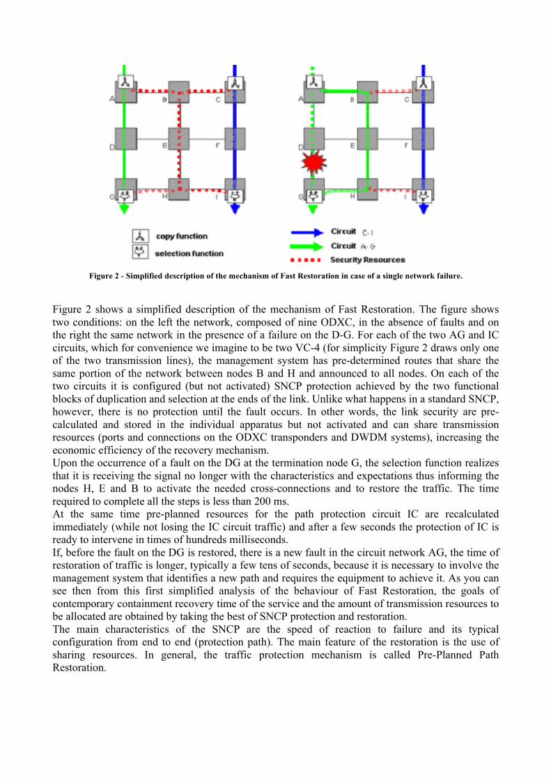
Figure 2 - Simplified description of the mechanism of Fast Restoration in case of a single network failure.

Figure 2 shows a simplified description of the mechanism of Fast Restoration. The figure shows two conditions: on the left the network, composed of nine ODXC, in the absence of faults and on the right the same network in the presence of a failure on the D-G. For each of the two AG and IC circuits, which for convenience we imagine to be two VC-4 (for simplicity Figure 2 draws only one of the two transmission lines), the management system has pre-determined routes that share the same portion of the network between nodes B and H and announced to all nodes. On each of the two circuits it is configured (but not activated) SNCP protection achieved by the two functional blocks of duplication and selection at the ends of the link. Unlike what happens in a standard SNCP, however, there is no protection until the fault occurs. In other words, the link security are pre-calculated and stored in the individual apparatus but not activated and can share transmission resources (ports and connections on the ODXC transponders and DWDM systems), increasing the economic efficiency of the recovery mechanism. Upon the occurrence of a fault on the DG at the termination node G, the selection function realizes that it is receiving the signal no longer with the characteristics and expectations thus informing the nodes H, E and B to activate the needed cross-connections and to restore the traffic. The time required to complete all the steps is less than 200 ms. At the same time pre-planned resources for the path protection circuit IC are recalculated immediately (while not losing the IC circuit traffic) and after a few seconds the protection of IC is ready to intervene in times of hundreds milliseconds. If, before the fault on the DG is restored, there is a new fault in the circuit network AG, the time of restoration of traffic is longer, typically a few tens of seconds, because it is necessary to involve the management system that identifies a new path and requires the equipment to achieve it. As you can see then from this first simplified analysis of the behaviour of Fast Restoration, the goals of contemporary containment recovery time of the service and the amount of transmission resources to be allocated are obtained by taking the best of SNCP protection and restoration. The main characteristics of the SNCP are the speed of reaction to failure and its typical configuration from end to end (protection path). The main feature of the restoration is the use of sharing resources. In general, the traffic protection mechanism is called Pre-Planned Path Restoration.

2.2. IP layer The Internet is often described as a network of networks, a global system of interconnected computer networks using the standardized Internet Protocol Suite. A connected group of one or more IP prefixes run by one or more network operators having a single and clearly defined routing policy is identified as an Autonomous System (AS). An AS shares routing information with other ASes using the Border Gateway Protocol (BGP). Establishing connections is driven more by business factors than attempts to optimize performance. As stated before, there are two main classes of connections: provider-customer and peer-to-peer. In the former, an AS (customer) pays another AS (provider) to obtain Internet access (transit). In the latter, two networks (peers) exchange traffic between each other’s customers for their mutual benefit. Peer-to-peer connections can be settlement-free or paid, depending on the ASes interacting and the type of contract stipulated. In this context, a peculiar role is played by Internet Exchange Points (IXPs). The former are physical infrastructures which allow ASes to exchange Internet traffic, usually by means of mutual peering agreements, leading to lower costs (and, sometimes, lower latency) than in up- stream provider-customer connections. An Internet AS-level topology can be easily described as an undirected graph: nodes represent ASes while edges indicate the presence of one or more BGP connections between two ASs. There are several sources of Internet AS-level topology data (datasets hereafter ) obtained by different projects obtained using different methodologies which yield quite dissimilar topological views of the Internet. Most of the studies rely either on BGP-based data or on traceroute experiments. In both cases, the datasets represent biased views of the actual topology and are also largely incomplete. To date, few efforts have been spent to provide a detailed analytical comparison of the most important topology properties extracted from the different data sources.

2.2.1. Measurement tools To date there is no specifically designed tool to derive topology information on the Internet, therefore researchers had to derive it using various indirect measurements that provide some information on the existence of ASes and the connections between them. Internet AS-level topology data collected within the framework of these projects were obtained by using different methodologies that yield quite different topological views of the Internet. To build the Internet AS-level topology, each project used different tools to gather data from the Internet. Some tools, based on traceroute measurements, take dynamical snapshots of the Internet by gathering a sequence of IP hops (via either UDP or ICMP probe packets) along the forward path from the source to a given destination. Other tools gather both static snapshots of the BGP routing tables and dynamic BGP data in the form of BGP message dumps (UPDATEs and WITHDRAWALs BGP messages). Data collected by the traceroute and BGP approaches are very reliable, but, unfortunately, they are largely incomplete. Datasets links can be gathered by three methodologies: • active probing: datasets are obtained by traceroute-like methods (e.g. CAIDA Ark [9] [10],

Dimes [11]); • passive measurement: it relies on an observation point within the network capturing live data

from a portion of the network (e.g. CAIDA AS relationships [9] [10], Robtex [12], IRL [13]); • public published information retrieval (e.g. Regional Internet Registries such as [14] ).

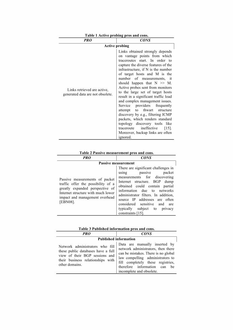
Table 1 Active probing pros and cons.

PRO CONS Active probing

Links retrieved are active, generated data are not obsolete.

Links obtained strongly depends on vantage points from which traceroutes start. In order to capture the diverse features of the infrastructure, if N is the number of target hosts and M is the number of measurements, it should happen that N >> M. Active probes sent from monitors to the large set of target hosts result in a significant traffic load and complex management issues. Service providers frequently attempt to thwart structure discovery by e.g., filtering ICMP packets, which renders standard topology discovery tools like traceroute ineffective [15]. Moreover, backup links are often ignored.

Table 2 Passive measurement pros and cons. PRO CONS

Passive measurement

Passive measurements of packet traffic offer the possibility of a greatly expanded perspective of Internet structure with much lower impact and management overhead [EBN08].

There are significant challenges in using passive packet measurements for discovering Internet structure. BGP dump obtained could contain partial information due to networks administrator filters. In addition, source IP addresses are often considered sensitive and are typically subject to privacy constraints [15].

Table 3 Published information pros and cons. PRO CONS

Published information

Network administrators who fill these public databases have a full view of their BGP sessions and their business relationships with other domains.

Data are manually inserted by network administrators, then there can be mistakes. There is no global law compelling administrators to fill completely these registries, therefore information can be incomplete and obsolete.

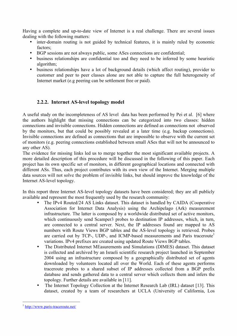
Having a complete and up-to-date view of Internet is a real challenge. There are several issues dealing with the following matters:

• inter-domain routing is not guided by technical features, it is mainly ruled by economic factors;

• BGP sessions are not always public, some ASes connections are confidential; • business relationships are confidential too and they need to be inferred by some heuristic

algorithm; • business relationships have a lot of background details (which affect routing), provider to

customer and peer to peer classes alone are not able to capture the full heterogeneity of Internet market (e.g peering can be settlement free or paid).

2.2.2. Internet AS-level topology model A useful study on the incompleteness of AS level data has been performed by Pei et al. [6] where the authors highlight that missing connections can be categorized into two classes: hidden connections and invisible connections. Hidden connections are defined as connections not observed by the monitors, but that could be possibly revealed at a later time (e.g. backup connections). Invisible connections are defined as connections that are impossible to observe with the current set of monitors (e.g. peering connections established between small ASes that will not be announced to any other AS). The evidence for missing links led us to merge together the most significant available projects. A more detailed description of this procedure will be discussed in the following of this paper. Each project has its own specific set of monitors, in different geographical locations and connected with different ASs. Thus, each project contributes with its own view of the Internet. Merging multiple data sources will not solve the problem of invisible links, but should improve the knowledge of the Internet AS-level topology. In this report three Internet AS-level topology datasets have been considered; they are all publicly available and represent the most frequently used by the research community:

• The IPv4 Routed/24 AS Links dataset. This dataset is handled by CAIDA (Cooperative Association for Internet Data Analysis) using the Archipelago (Ark) measurement infrastructure. The latter is composed by a worldwide distributed set of active monitors, which continuously send Scamper3 probes to destination IP addresses, which, in turn, are connected to a central server. Next, the IP addresses found are mapped to AS numbers with Route Views BGP tables and the AS-level topology is retrieved. Probes are carried out by TCP-, UDP-, and ICMP-based measurements and Paris traceroute1 variations. IPv4 prefixes are created using updated Route Views BGP tables.

• The Distributed Internet MEasurements and Simulations (DIMES) dataset. This dataset is collected and archived by an Israeli scientific research project launched in September 2004 using an infrastructure composed by a geographically distributed set of agents downloaded by volunteers located all over the World. Each of these agents performs traceroute probes to a shared subset of IP addresses collected from a BGP prefix database and sends gathered data to a central server which collects them and infers the topology. Further details are available in [11].

• The Internet Topology Collection at the Internet Research Lab (IRL) dataset [13]. This dataset, created by a team of researchers at UCLA (University of California, Los

1 http://www.paris-traceroute.net/

Angeles) , infers the topology using BGP routing tables and UPDATEs collected by several ongoing projects (i.e. Route Views, RIPE Routing Information Service (RIS), Abilene and collecting BGP data through route and looking glass servers.

The above three datasets were originally built using two different methodologies. In the MOTIA Activity II all the collected data have been merged using the same methodology; thus forming two different datasets referred to as:

• Traceroutes: the union of DIMES and CAIDA datasets, • BGP: the IRL dataset.

In addition, in this paper we often use the following dataset:

• Merge: the fusion of DIMES, CAIDA and IRL datasets. It is worth noting that all data gathered from each of the projects were analyzed and controlled ( a data hygiene process was performed) before being regarded as correct. Specifically, as a result of such screening, the following have been removed from the resulting topology:

• ASNs declared as private by IANA, • AS 23456 which, according to RFC 4893 is reserved and assigned for AS_TRANS, • AS 3130 which, according to the Cyclops website, shows false AS adjacencies due to an

experiment by Randy Bush. Comparing the DIMES and CAIDA traceroute-derived graphs, we can see that the sets of their constituent connections are quite different, i.e. 51.9% of connections are common to both datasets, while 22.4% are only present in CAIDA, and 25.7% are only present in DIMES. From the above considerations, we can draw the following conclusions:

a) both datasets enrich the Traceroutes dataset; b) measuring procedures using the same tool (traceroute) can lead to substantially different

results. Hereafter the topologies inferred from Traceroutes, BGP and Merge datasets will be referred to as Traceroutes, BGP and Merge ‘‘topologies”, respectively. Furthermore, we will still continue to use the expressions Traceroutes and BGP ‘‘methodologies”.

Table 4 - Comparison of topology datasets.

Dataset Number of nodes Number of connections TRACEROUTES 28821 73271

BGP 37258 121634 MERGE 37258 144416

By analyzing the number of nodes in Table 1, we can observe that traceroute-based methods are able to discover a smaller number of ASes compared to BGP methods, while a very limited number of nodes (27 out of 34,955) were discovered by Traceroutes methods, but not by BGP methods. An analysis of the number of connections indicates that Traceroutes and BGP complement each other very well (e.g. Traceroutes increases the number of connections discovered by BGP by about 20%). Only 37.6% of the connections in the Merge dataset were discovered by both methods, while the remaining 62.4% of the connections was discovered either by the Traceroutes (21.9%) or by the BGP (40.5%) methods.

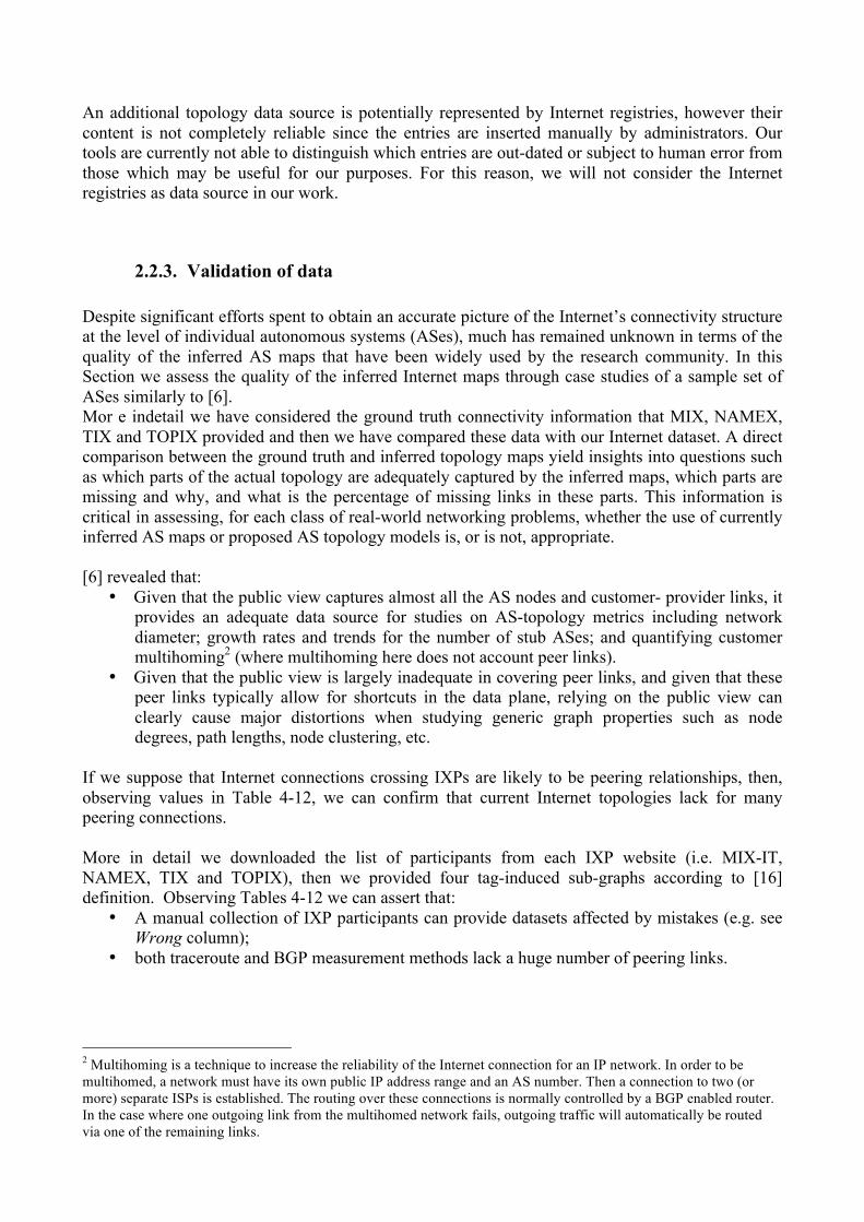
An additional topology data source is potentially represented by Internet registries, however their content is not completely reliable since the entries are inserted manually by administrators. Our tools are currently not able to distinguish which entries are out-dated or subject to human error from those which may be useful for our purposes. For this reason, we will not consider the Internet registries as data source in our work.

2.2.3. Validation of data Despite significant efforts spent to obtain an accurate picture of the Internet’s connectivity structure at the level of individual autonomous systems (ASes), much has remained unknown in terms of the quality of the inferred AS maps that have been widely used by the research community. In this Section we assess the quality of the inferred Internet maps through case studies of a sample set of ASes similarly to [6]. Mor e indetail we have considered the ground truth connectivity information that MIX, NAMEX, TIX and TOPIX provided and then we have compared these data with our Internet dataset. A direct comparison between the ground truth and inferred topology maps yield insights into questions such as which parts of the actual topology are adequately captured by the inferred maps, which parts are missing and why, and what is the percentage of missing links in these parts. This information is critical in assessing, for each class of real-world networking problems, whether the use of currently inferred AS maps or proposed AS topology models is, or is not, appropriate. [6] revealed that:

• Given that the public view captures almost all the AS nodes and customer- provider links, it provides an adequate data source for studies on AS-topology metrics including network diameter; growth rates and trends for the number of stub ASes; and quantifying customer multihoming2 (where multihoming here does not account peer links).

• Given that the public view is largely inadequate in covering peer links, and given that these peer links typically allow for shortcuts in the data plane, relying on the public view can clearly cause major distortions when studying generic graph properties such as node degrees, path lengths, node clustering, etc.

If we suppose that Internet connections crossing IXPs are likely to be peering relationships, then, observing values in Table 4-12, we can confirm that current Internet topologies lack for many peering connections. More in detail we downloaded the list of participants from each IXP website (i.e. MIX-IT, NAMEX, TIX and TOPIX), then we provided four tag-induced sub-graphs according to [16] definition. Observing Tables 4-12 we can assert that:

• A manual collection of IXP participants can provide datasets affected by mistakes (e.g. see Wrong column);

• both traceroute and BGP measurement methods lack a huge number of peering links.

2 Multihoming is a technique to increase the reliability of the Internet connection for an IP network. In order to be multihomed, a network must have its own public IP address range and an AS number. Then a connection to two (or more) separate ISPs is established. The routing over these connections is normally controlled by a BGP enabled router. In the case where one outgoing link from the multihomed network fails, outgoing traffic will automatically be routed via one of the remaining links.

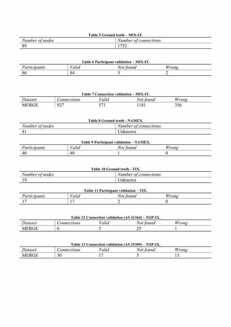
Table 5 Ground truth – MIX-IT.

Number of nodes Number of connections 89 1752

Table 6 Participant validation – MIX-IT. Participants Valid Not found Wrong 86 84 5 2

Table 7 Connection validation – MIX-IT. Dataset Connections Valid Not found Wrong MERGE 927 571 1181 356

Table 8 Ground truth - NAMEX. Number of nodes Number of connections 41 Unknown

Table 9 Participant validation – NAMEX. Participants Valid Not found Wrong 40 40 1 0

Table 10 Ground truth - TIX. Number of nodes Number of connections 19 Unknown

Table 11 Participant validation – TIX. Participants Valid Not found Wrong 17 17 2 0

Table 12 Connection validation (AS 41364) – TOP-IX. Dataset Connections Valid Not found Wrong MERGE 6 5 25 1

Table 13 Connection validation (AS 25309) – TOP-IX. Dataset Connections Valid Not found Wrong MERGE 30 17 5 13

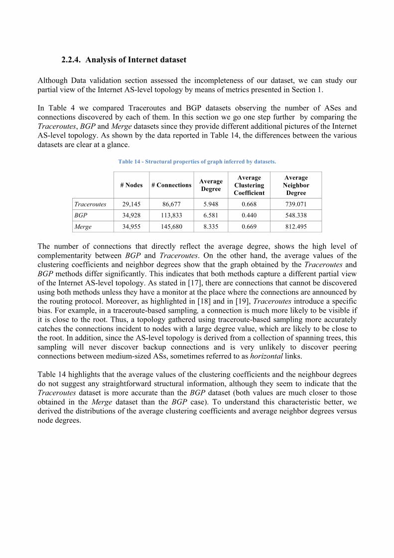
2.2.4. Analysis of Internet dataset Although Data validation section assessed the incompleteness of our dataset, we can study our partial view of the Internet AS-level topology by means of metrics presented in Section 1. In Table 4 we compared Traceroutes and BGP datasets observing the number of ASes and connections discovered by each of them. In this section we go one step further by comparing the Traceroutes, BGP and Merge datasets since they provide different additional pictures of the Internet AS-level topology. As shown by the data reported in Table 14, the differences between the various datasets are clear at a glance.

Table 14 - Structural properties of graph inferred by datasets.

# Nodes # Connections Average Degree

Average Clustering Coefficient

Average Neighbor

Degree

Traceroutes 29,145 86,677 5.948 0.668 739.071

BGP 34,928 113,833 6.581 0.440 548.338

Merge 34,955 145,680 8.335 0.669 812.495

The number of connections that directly reflect the average degree, shows the high level of complementarity between BGP and Traceroutes. On the other hand, the average values of the clustering coefficients and neighbor degrees show that the graph obtained by the Traceroutes and BGP methods differ significantly. This indicates that both methods capture a different partial view of the Internet AS-level topology. As stated in [17], there are connections that cannot be discovered using both methods unless they have a monitor at the place where the connections are announced by the routing protocol. Moreover, as highlighted in [18] and in [19], Traceroutes introduce a specific bias. For example, in a traceroute-based sampling, a connection is much more likely to be visible if it is close to the root. Thus, a topology gathered using traceroute-based sampling more accurately catches the connections incident to nodes with a large degree value, which are likely to be close to the root. In addition, since the AS-level topology is derived from a collection of spanning trees, this sampling will never discover backup connections and is very unlikely to discover peering connections between medium-sized ASs, sometimes referred to as horizontal links. Table 14 highlights that the average values of the clustering coefficients and the neighbour degrees do not suggest any straightforward structural information, although they seem to indicate that the Traceroutes dataset is more accurate than the BGP dataset (both values are much closer to those obtained in the Merge dataset than the BGP case). To understand this characteristic better, we derived the distributions of the average clustering coefficients and average neighbor degrees versus node degrees.

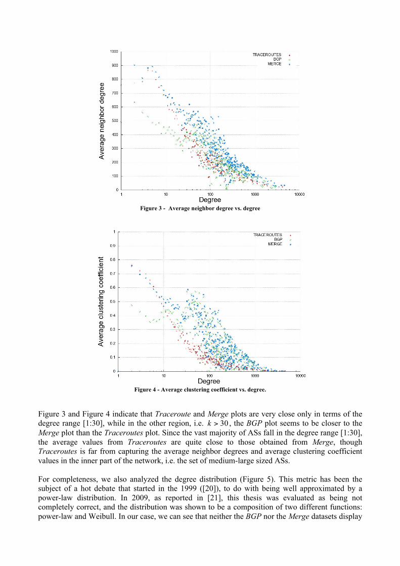
Figure 3 - Average neighbor degree vs. degree

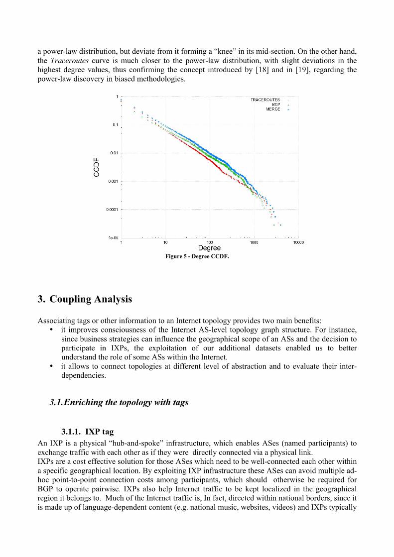
Figure 4 - Average clustering coefficient vs. degree.

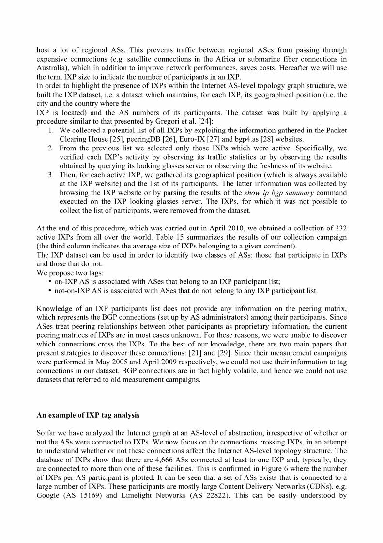
Figure 3 and Figure 4 indicate that Traceroute and Merge plots are very close only in terms of the degree range [1:30], while in the other region, i.e. , the BGP plot seems to be closer to the Merge plot than the Traceroutes plot. Since the vast majority of ASs fall in the degree range [1:30], the average values from Traceroutes are quite close to those obtained from Merge, though Traceroutes is far from capturing the average neighbor degrees and average clustering coefficient values in the inner part of the network, i.e. the set of medium-large sized ASs. For completeness, we also analyzed the degree distribution (Figure 5). This metric has been the subject of a hot debate that started in the 1999 ([20]), to do with being well approximated by a power-law distribution. In 2009, as reported in [21], this thesis was evaluated as being not completely correct, and the distribution was shown to be a composition of two different functions: power-law and Weibull. In our case, we can see that neither the BGP nor the Merge datasets display

a power-law distribution, but deviate from it forming a “knee” in its mid-section. On the other hand, the Traceroutes curve is much closer to the power-law distribution, with slight deviations in the highest degree values, thus confirming the concept introduced by [18] and in [19], regarding the power-law discovery in biased methodologies.

Figure 5 - Degree CCDF.

3. Coupling Analysis Associating tags or other information to an Internet topology provides two main benefits:

• it improves consciousness of the Internet AS-level topology graph structure. For instance, since business strategies can influence the geographical scope of an ASs and the decision to participate in IXPs, the exploitation of our additional datasets enabled us to better understand the role of some ASs within the Internet.

• it allows to connect topologies at different level of abstraction and to evaluate their inter-dependencies.

3.1. Enriching the topology with tags

3.1.1. IXP tag An IXP is a physical “hub-and-spoke” infrastructure, which enables ASes (named participants) to exchange traffic with each other as if they were directly connected via a physical link. IXPs are a cost effective solution for those ASes which need to be well-connected each other within a specific geographical location. By exploiting IXP infrastructure these ASes can avoid multiple ad-hoc point-to-point connection costs among participants, which should otherwise be required for BGP to operate pairwise. IXPs also help Internet traffic to be kept localized in the geographical region it belongs to. Much of the Internet traffic is, In fact, directed within national borders, since it is made up of language-dependent content (e.g. national music, websites, videos) and IXPs typically

host a lot of regional ASs. This prevents traffic between regional ASes from passing through expensive connections (e.g. satellite connections in the Africa or submarine fiber connections in Australia), which in addition to improve network performances, saves costs. Hereafter we will use the term IXP size to indicate the number of participants in an IXP. In order to highlight the presence of IXPs within the Internet AS-level topology graph structure, we built the IXP dataset, i.e. a dataset which maintains, for each IXP, its geographical position (i.e. the city and the country where the IXP is located) and the AS numbers of its participants. The dataset was built by applying a procedure similar to that presented by Gregori et al. [24]:

1. We collected a potential list of all IXPs by exploiting the information gathered in the Packet Clearing House [25], peeringDB [26], Euro-IX [27] and bgp4.as [28] websites.

2. From the previous list we selected only those IXPs which were active. Specifically, we verified each IXP’s activity by observing its traffic statistics or by observing the results obtained by querying its looking glasses server or observing the freshness of its website.

3. Then, for each active IXP, we gathered its geographical position (which is always available at the IXP website) and the list of its participants. The latter information was collected by browsing the IXP website or by parsing the results of the show ip bgp summary command executed on the IXP looking glasses server. The IXPs, for which it was not possible to collect the list of participants, were removed from the dataset.

At the end of this procedure, which was carried out in April 2010, we obtained a collection of 232 active IXPs from all over the world. Table 15 summarizes the results of our collection campaign (the third column indicates the average size of IXPs belonging to a given continent). The IXP dataset can be used in order to identify two classes of ASs: those that participate in IXPs and those that do not. We propose two tags:

• on-IXP AS is associated with ASes that belong to an IXP participant list; • not-on-IXP AS is associated with ASes that do not belong to any IXP participant list.

Knowledge of an IXP participants list does not provide any information on the peering matrix, which represents the BGP connections (set up by AS administrators) among their participants. Since ASes treat peering relationships between other participants as proprietary information, the current peering matrices of IXPs are in most cases unknown. For these reasons, we were unable to discover which connections cross the IXPs. To the best of our knowledge, there are two main papers that present strategies to discover these connections: [21] and [29]. Since their measurement campaigns were performed in May 2005 and April 2009 respectively, we could not use their information to tag connections in our dataset. BGP connections are in fact highly volatile, and hence we could not use datasets that referred to old measurement campaigns. An example of IXP tag analysis So far we have analyzed the Internet graph at an AS-level of abstraction, irrespective of whether or not the ASs were connected to IXPs. We now focus on the connections crossing IXPs, in an attempt to understand whether or not these connections affect the Internet AS-level topology structure. The database of IXPs show that there are 4,666 ASs connected at least to one IXP and, typically, they are connected to more than one of these facilities. This is confirmed in Figure 6 where the number of IXPs per AS participant is plotted. It can be seen that a set of ASs exists that is connected to a large number of IXPs. These participants are mostly large Content Delivery Networks (CDNs), e.g. Google (AS 15169) and Limelight Networks (AS 22822). This can be easily understood by

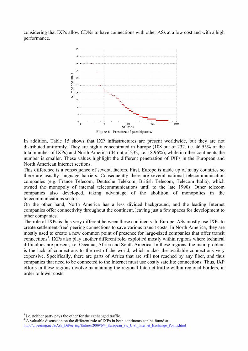
considering that IXPs allow CDNs to have connections with other ASs at a low cost and with a high performance.

Figure 6 –Presence of participants.

In addition, Table 15 shows that IXP infrastructures are present worldwide, but they are not distributed uniformly. They are highly concentrated in Europe (108 out of 232, i.e. 46.55% of the total number of IXPs) and North America (44 out of 232, i.e. 18.96%), while in other continents the number is smaller. These values highlight the different penetration of IXPs in the European and North American Internet sections. This difference is a consequence of several factors. First, Europe is made up of many countries so there are usually language barriers. Consequently there are several national telecommunication companies (e.g. France Telecom, Deutsche Telekom, British Telecom, Telecom Italia), which owned the monopoly of internal telecommunications until to the late 1990s. Other telecom companies also developed, taking advantage of the abolition of monopolies in the telecommunications sector. On the other hand, North America has a less divided background, and the leading Internet companies offer connectivity throughout the continent, leaving just a few spaces for development to other companies. The role of IXPs is thus very different between these continents. In Europe, ASs mostly use IXPs to create settlement-free3 peering connections to save various transit costs. In North America, they are mostly used to create a new common point of presence for large-sized companies that offer transit connections4. IXPs also play another different role, exploited mostly within regions where technical difficulties are present, i.e. Oceania, Africa and South America. In these regions, the main problem is the lack of connections to the rest of the world, which makes the available connections very expensive. Specifically, there are parts of Africa that are still not reached by any fiber, and thus companies that need to be connected to the Internet must use costly satellite connections. Thus, IXP efforts in these regions involve maintaining the regional Internet traffic within regional borders, in order to lower costs.

3 i.e. neither party pays the other for the exchanged traffic. 4 A valuable discussion on the different role of IXPs in both continents can be found at http://drpeering.net/a/Ask_DrPeering/Entries/2009/6/4_European_vs._U.S._Internet_Exchange_Points.html

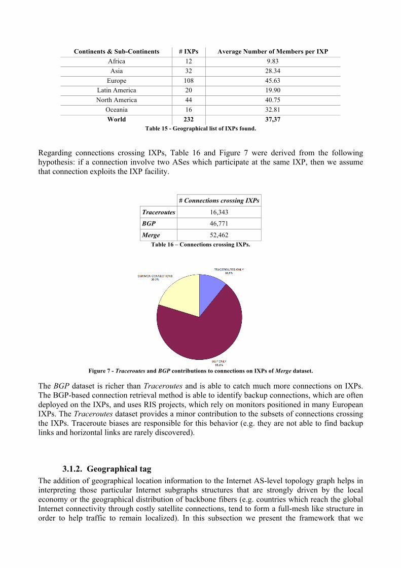
Continents & Sub-Continents # IXPs Average Number of Members per IXP Africa 12 9.83 Asia 32 28.34

Europe 108 45.63 Latin America 20 19.90 North America 44 40.75

Oceania 16 32.81 World 232 37,37

Table 15 - Geographical list of IXPs found.

Regarding connections crossing IXPs, Table 16 and Figure 7 were derived from the following hypothesis: if a connection involve two ASes which participate at the same IXP, then we assume that connection exploits the IXP facility.

# Connections crossing IXPs

Traceroutes 16,343

BGP 46,771

Merge 52,462 Table 16 – Connections crossing IXPs.

Figure 7 - Traceroutes and BGP contributions to connections on IXPs of Merge dataset.

The BGP dataset is richer than Traceroutes and is able to catch much more connections on IXPs. The BGP-based connection retrieval method is able to identify backup connections, which are often deployed on the IXPs, and uses RIS projects, which rely on monitors positioned in many European IXPs. The Traceroutes dataset provides a minor contribution to the subsets of connections crossing the IXPs. Traceroute biases are responsible for this behavior (e.g. they are not able to find backup links and horizontal links are rarely discovered).

3.1.2. Geographical tag The addition of geographical location information to the Internet AS-level topology graph helps in interpreting those particular Internet subgraphs structures that are strongly driven by the local economy or the geographical distribution of backbone fibers (e.g. countries which reach the global Internet connectivity through costly satellite connections, tend to form a full-mesh like structure in order to help traffic to remain localized). In this subsection we present the framework that we

developed to associate a list of geographical location with each AS by exploiting the MaxMind IP geolocation service. The following this procedure was used to build the geographical dataset: 1. We downloaded the GeoLite Country and the GeoLite ASN free databases from MaxMind website9. Both of them were uploaded on 1 May 2010. The GeoLite Country database associates IPv4 addresses with country codes. The GeoLite ASN database maps IPv4 addresses to AS numbers. 2. We merged the GeoLite Country and the Geolite ASN databases using the IPv4 address field. Thus, we obtained a database containing < AS number, Country code > tuples. Note that, for each AS number multiple country codes could exist, hence the geographical database key is the entire tuple. The resulting geographical database associates 34,190 ASes with at least one country code. In Section 4 we provide a geographic attribute to each AS, according to the following taxonomy:

• An AS is called a national AS if all of its geographical locations belong to the same country, i.e. its networks are placed within a single country.

• An AS is called a continental AS if all of its geographical locations are placed within the same continent. For example, an AS is called European if its geographical locations belong to European countries and none of its geographical locations are placed outside Europe.

• An AS is called a worldwide AS if it owns at least two geographical locations which are located in two different continents. For example, an AS which has one geographical location in the Netherlands and one geographical location in the United States is referred to as worldwide AS.

3.1.3. Business tag In the literature, economic relationships between ASes are usually classified as customer-provider, peer-to-peer and sibling-to-sibling [30][31]. In the customer- provider agreement, an AS (customer) pays another AS (provider) to obtain connectivity to the rest of the Internet. In the peer-to-peer agreement, a pair of ASes (peers) agree to exchange traffic between their respective customers, typically free of charge. In the sibling-to-sibling agreement a pair of ASes (siblings) provide each other with connectivity to the rest of the Internet.

3.2. Linking multiple layers A key aspect of understanding and analysing network is to accurately represent the topology of the existing network, as well as to be able to generate representative alternative topologies to evaluate resilience properties, and to be the basis of comparing candidate mechanisms. The majority of topology modelling is based on logical topologies focusing on the generation of either router-level or AS-level topologies, motivated by the desire to study Internet layer-3 connectivity and protocols such IP, BGP, and IGPs, constrained by the fact that the majority of inference mechanisms are only able to collect data on the router-level connectivity of commercial networks. However, a router-level topology is an abstraction of the underlying physical topology and not an exact representation. Links visible to layer 3 are logical interconnections consisting of multiple physical links between layer 2 and layer 1 components such as switches, multiplexers, regenerators, and optical amplifiers. Furthermore, layer 3 topologies are frequently not representative of the underlying infrastructure due to layer 2.5 technologies such as MPLS, SONET, and Metro Ethernet that permit rearrangement of paths for traffic engineering, policy, and restoration.

Linking the application layer and network layer is not a simple process. There are some cases in which single IP cannot locate a single machine; for example, a NAT could hide a large network of hosts. In addition, even if the couple IP address – Port number is given, the service requested could be managed by a set of different hosts. However IP address and port play a key role in linking the IP networking infrastructure and the application layer distributed system and provide a key role in linking the application process to the network. Our idea is to start using the IP only. In the second phase we can add the port descriptor but this will require the port information that must be acquired with direct measurements. This work is not technically difficult as the port is well specified in the TCP or UDP header but it an ad hoc measure for the application service under study and hence can be acquired in specific case studies only. As a possible last further step is to add the description of the distributed computing system that can be reached by the coupe IP address, Port number.

Bibliography

[1] R. Albert, A.-L. Barabasi, Rev. Mod. Phys., 74 (2002) 47. [2] S. Boccaletti et al., Phys. Reports, 424 (2006) 175. [3] L.A.N. Amaral et al., Proc. Nat. Acad. Sci. USA, 97 (2000) 11149. [4] Romualdo Pastor-Satorras and Alessandro Vespignani. Evolution and Structure of the

Internet: A Statistical Physics Approach. Cambridge University Press, New York, NY, USA, 2004.

[5] R. Albert, A.-L. Barabási, Topology of evolving networks: Local events and universality. Physical Review Letters, 85(24):5234+, December 2000.

[6] D. Pei, W. Willinger, B. Zhang, L. Zhang, R.V. Oliveira, The (in)completeness of the observed Internet AS-level structure, IEEE/ACM Transactions on Networking (TON) 18 (1) (2010) 109–122.

[7] Gunnar Carlsson. Topology and data. Bulletin of the American Mathematical Society, 46(2):255–308, January 2009. ISSN 0273- 0979. doi: 10.1090/S0273-0979-09-01249-X. URL http://www. ams.org/journal-getitem?pii=S0273-0979-09-01249-X.

[8] F. M. Dong, K. M. Koh, and K. L. Teo. Chromatic polynomials and chromaticity of graphs. World Scientific Publishing Co. Pte. Ltd., 2005. ISBN 9812563172.

[9] The cooperative association for internet data analysis, 2009. [Online; accessed 06-August-2009; http://www.caida.org/home/].

[10] Young Hyun, Bradley Huffaker, Dan Andersen, Emile Aben, Colleen Shannon, Matthew Luckie, and kc claffy. The CAIDA IPv4 Routed /24 Topology Dataset, 2009. [Online; accessed 24- August-2009; http://www.caida.org/data/active/ipv4_routed_24_ topology_dataset.xml].

[11] Yuval Shavitt and Eran Shir. Dimes: let the internet measure itself. Computer Communication Review, 35(5):71–74, 2005.

[12] robtex.com, 2009. [Online; accessed 06-August-2009; http://www. robtex.com/]. [13] Internet Research Lab, UCLA. http://irl.cs.ucla.edu/ [14] RIPE Regional Internet Registry, 2009. [Online; accessed 07-August- 2009;

http://www.ripe.net/]. [15] Brian Eriksson, Paul Barford, and Robert Nowak. Network discovery from passive

measurements. SIGCOMM Comput. Commun. Rev., 38(4):291–302, 2008. [16] G. Palla, I. J. Farkas, P. Pollner, I. Dernyi, and T. Vicsek, “Fundamental statistical features

and self-similar properties of tagged networks,” New Journal of Physics, vol. 10, no. 12, p. 123026, 2008.

[17] D. Pei, W. Willinger, B. Zhang, L. Zhang and R.V. Oliveira, “In search of the elusive ground truth: the Internet’s AS-level connectivity structure”, in ACM SIGMETRICS Performance Evaluation Review, 2008, vol. 36, pp. 217-228.

[18] J. W. Byers, M. Crovella, P. Xie and A. Lakhina, “Sampling biases in IP topology measurements”, in Proc. IEEE INFOCOM, 2003, pp 332-341.

[19] A. Clauset, D. Kempe, C. Moore and D. Achlioptas, “On the bias of traceroute sampling: or, power-law degree distributions in regular graphs”, in Proc. ACM STOC, 2005, pp. 694-703.

[20] M. Faloutsos, P. Faloutsos and C. Faloutsos, “On power-law relationships of the Internet topology”, in Proc. ACM SIGCOMM, 1999, pp. 251-262.

[21] G. Siganos, M. Faloutsos, S. Krishnamurthy and Y. He, “Lord of the links: a framework for discovering missing links in the Internet topology”, in IEEE/ACM Trans. Networking, 2009, vol. 17, pp. 391-404.

[22] Neil Spring, Ratul Mahajan, and David Wetherall. Measuring ISP Topologies with Rocketfuel. SIGCOMM 2002.

[23] Yuval Shavitt and Noa Zilberman. A Structural Approach for PoP Geo-Location. NetSciCom, March 2010, San Diego, CA, USA.

[24] Gregori, E., Improta, A., Lenzini, L., Orsini, C.: The impact of IXPs on the AS-level topology structure of the internet. Computer Communications (2010)

[25] Packet Clearing House (PCH) http://www.pch.net/ [26] PeeringDB https://www.peeringdb.com/ [27] European Internet Exchange Association http://www.euro-ix.net/ [28] BGP: the Border Gateway Protocol Advanced Internet Routing Resources

http://www.bgp4.as/ [29] B. Augustin, B. Krishnamurthy, and W. Willinger, “IXPs: mapped?” in IMC ’09:

Proceedings of the 9th ACM SIGCOMM conference on Internet measurement conference, 2009, pp. 336–349.

[30] Huston, G.: Interconnection, peering, and settlements. INET’99 Abstracts Book (1999) [31] Gao, L.: On inferring autonomous system relationships in the internet. IEEE/ACM

TRANSACTIONS ON NETWORKING 9(6), 733–745 (Dec 2001)