M4 Deliverable Report

M4

De

liv

er

ab

le

Re

po

rt

http://www.m4project.org/

http://www.m4project.org/

Final Report on MultimodalRecognizers

M4 Deliverable D2.2

10 March 2005

Project Ref. No. IST 2001-34485Project Acronym M4Project Full Title MultiModal Meeting ManagerSecurity RestrictedContractual Date of Delivery 28 February 2005Actual Date of Delivery 10 March 2005Deliverable Number D2.2Deliverable Name Final Report on Multimodal RecognizersType ReportWP Contributing to Deliverable WP2WP/Task Responsible TUMOther Contributors USFD, EPFL, IDIAP, TNO, UT, VUTEditors S. Reiter, G. RigollEC Project Officer Domenico PerottaKeywords Multimodal recognizers, speech recognition, gesture

recognition, tracking, person identification, localiza-tion.

Abstract This report gives a report of the developed methodsand techniques of multimodal recognizers that areused in the M4 domain. This includes the descriptionof recognizers in the auditory domain, like phonemerecognition and localization, the video domain, repre-sented by gesture recognition, person identification,person tracking and gaze tracking, and multimodalmultimodal approaches for tracking and localizationof people. The outcome of these approaches give asufficient input for the more higher level approachesin WP3 for efficient meeting analysis and multimodalaccess.

M4 Deliverable D2.2 1

Contents

1 Introduction 31.1 Involved Partners . . . . . . . . . . . . . . . . . . . . . . . . . . . . . . . . . . 31.2 Areas of work . . . . . . . . . . . . . . . . . . . . . . . . . . . . . . . . . . . . 31.3 Aim in the last year and Outline of this Deliverable . . . . . . . . . . . . . . 3

2 Audio processing 52.1 Phoneme recognition . . . . . . . . . . . . . . . . . . . . . . . . . . . . . . . . 5

2.1.1 Split-context system . . . . . . . . . . . . . . . . . . . . . . . . . . . . 52.1.2 Experiments . . . . . . . . . . . . . . . . . . . . . . . . . . . . . . . . 62.1.3 Applications of phoneme recognition and posteriors estimation . . . . 7

2.2 Feature extraction and training of HMM recognition systems . . . . . . . . . 82.2.1 Features and transforms . . . . . . . . . . . . . . . . . . . . . . . . . . 82.2.2 SERest – new HMM training tool . . . . . . . . . . . . . . . . . . . . . 9

2.3 Large Vocabulary Speech Recognition . . . . . . . . . . . . . . . . . . . . . . 92.4 Use of microphone arrays . . . . . . . . . . . . . . . . . . . . . . . . . . . . . 11

2.4.1 Introduction . . . . . . . . . . . . . . . . . . . . . . . . . . . . . . . . 112.4.2 Enhancement Technique . . . . . . . . . . . . . . . . . . . . . . . . . . 122.4.3 Array Geometry . . . . . . . . . . . . . . . . . . . . . . . . . . . . . . 122.4.4 Data Collection . . . . . . . . . . . . . . . . . . . . . . . . . . . . . . . 132.4.5 Experiments and Results . . . . . . . . . . . . . . . . . . . . . . . . . 14

2.5 Localization and Speaker Segmentation . . . . . . . . . . . . . . . . . . . . . 152.5.1 Introduction . . . . . . . . . . . . . . . . . . . . . . . . . . . . . . . . 152.5.2 Supervised Location-Based Segmentation . . . . . . . . . . . . . . . . 162.5.3 Data Collection: the AV16.3 corpus . . . . . . . . . . . . . . . . . . . 162.5.4 Sector-Based Detection and Localization . . . . . . . . . . . . . . . . . 172.5.5 Unsupervised Location-Based Segmentation . . . . . . . . . . . . . . . 17

2.6 Localization and tracking of multiple speakers simultaneously . . . . . . . . . 182.6.1 Introduction . . . . . . . . . . . . . . . . . . . . . . . . . . . . . . . . 182.6.2 Numerical simulations . . . . . . . . . . . . . . . . . . . . . . . . . . . 182.6.3 Experiments . . . . . . . . . . . . . . . . . . . . . . . . . . . . . . . . 182.6.4 Conclusion . . . . . . . . . . . . . . . . . . . . . . . . . . . . . . . . . 19

3 Video processing 213.1 Mobile USB 2.0 Camera . . . . . . . . . . . . . . . . . . . . . . . . . . . . . . 21

3.1.1 Hardware . . . . . . . . . . . . . . . . . . . . . . . . . . . . . . . . . . 213.1.2 Software . . . . . . . . . . . . . . . . . . . . . . . . . . . . . . . . . . . 24

3.2 Sequential Monte Carlo framework . . . . . . . . . . . . . . . . . . . . . . . . 263.3 Face detection . . . . . . . . . . . . . . . . . . . . . . . . . . . . . . . . . . . . 263.4 Person Tracking . . . . . . . . . . . . . . . . . . . . . . . . . . . . . . . . . . . 283.5 Person tracking using omnidirectional view . . . . . . . . . . . . . . . . . . . 29

3.5.1 Tranformation omnidirectional view . . . . . . . . . . . . . . . . . . . 293.5.2 Hand and face tracking . . . . . . . . . . . . . . . . . . . . . . . . . . 313.5.3 Mouth localization in low resolution image . . . . . . . . . . . . . . . 33

3.6 Tracking multiple people . . . . . . . . . . . . . . . . . . . . . . . . . . . . . . 34

2 M4 Deliverable D2.2

3.7 Tracking head pose . . . . . . . . . . . . . . . . . . . . . . . . . . . . . . . . . 353.8 Person action recognition . . . . . . . . . . . . . . . . . . . . . . . . . . . . . 36

4 Multimodal recognizers 394.1 Audio-visual tracking using SMC-methods . . . . . . . . . . . . . . . . . . . . 394.2 Audio-visual localization and tracking using neurobiological methods . . . . . 40

4.2.1 Introduction . . . . . . . . . . . . . . . . . . . . . . . . . . . . . . . . 404.2.2 Audio cues . . . . . . . . . . . . . . . . . . . . . . . . . . . . . . . . . 424.2.3 Video cues . . . . . . . . . . . . . . . . . . . . . . . . . . . . . . . . . 424.2.4 Audio-visual integration . . . . . . . . . . . . . . . . . . . . . . . . . . 434.2.5 Object tracking . . . . . . . . . . . . . . . . . . . . . . . . . . . . . . . 44

References 45


1 Introduction

WP2 is concerned with the development, evaluation and improvement of multimodal recog-nizers for the different input modalities that transform the raw audio and video streams to“higher level” streams. These “higher level” streams will form the basis for the integrationand information access operations in WP3. Among these modalities are robust conversa-tional speech recognition, action and gesture recognition, emotion and intent recognition,source localization and tracking, and multimodal gesture recognition. Different versions ofthese components exist in various kinds and are available to the M4 partners. Due to thefact that these techniques are often based on similar or complementary tools, this providedgood opportunities for collaboration.

1.1 Involved Partners

Table 1 shows the involved partners and person-months in WP2.

Partner USFD EPFL TUM IDIAP TNO UNIGE UT VUT UEDINPMnth. 21 12 30 18 4 0 4 60 0

Table 1: Involved partners and person-months in WP2

1.2 Areas of work

The work in WP2 is divided into six sub-categories. These areas are:

• Robust Conversational speech recognition

• Language- and task-independent speech processing

• Action/gesture recognition

• Emotion/intent recognition

• Source localization and tracking

• Multimodal person identification

1.3 Aim in the last year and Outline of this Deliverable

The expected result of WP2 is a set of multimodal recognizers for robust speech recognitionfor meetings, gesture and action recognition, emotion recognition, source localization, objecttracking, and person identification. In the last three years we developed and ported a widerange of algorithms to the M4 domain.

The purpose of this document is to report about the progress that has been made inporting and implementing these algorithms for audio, video, and multimodal algorithms forM4. The methods are described in detail in Section 2 - 4.



2 Audio processing

Processing the audio signals is one of the crucial points in the analysis of meetings. Mostinformation in a meeting is transported via speech. So it is naturally that one of the mainfocusses must be speech recognition. This is done by various approaches using phonemerecognition or microphone arrays. But the audio channel can also be used for localizationand tracking of people as shown later in this section.

2.1 Phoneme recognition

The core of the work of Brno speech processing group within M4 was the phoneme recognitionand phoneme posterior probabilities estimation.

We believe that a system that would (without use of any prior information from thelanguage model) reliably yield a string or lattice of phoneme-like symbols that describe speechsounds, could be of a significant utility for deriving information about the message in speech,as well as in identification of the speaker and the language used. Since the symbol stringswould be derived without use of any language constraints, they can be of considerable utilityin spotting important and unexpected key-words in the conversation. From technical pointof view, phoneme strings/lattices are much more suitable form to store speech than waveformand the following algorithms can benefit from this compact symbolic representation.

To summarize our work on phoneme recognition, we have:

• built a system for phoneme recognition based on artificial neural nets that is comparableto the state-of-the-art (comparison on TIMIT database).

• extended the system for phoneme recognition of spontaneous meeting data and evalu-ated its performances on ICSI corpus.

• successfully used phoneme-posteriors as features at the input of GMM/HMM systemfor large vocabulary speech recognition.

• tested phoneme posteriors and phoneme lattices in systems for keyword spotting.

• evaluated phoneme recognizer as tokenizer in a system for language identification.

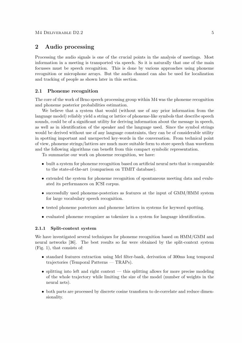
2.1.1 Split-context system

We have investigated several techniques for phoneme recognition based on HMM/GMM andneural networks [36]. The best results so far were obtained by the split-context system(Fig. 1), that consists of:

• standard features extraction using Mel filter-bank, derivation of 300ms long temporaltrajectories (Temporal Patterns — TRAPs).

• splitting into left and right context — this splitting allows for more precise modelingof the whole trajectory while limiting the size of the model (number of weights in theneural nets).

• both parts are processed by discrete cosine transform to de-correlate and reduce dimen-sionality.


• two neural nets are trained to produce the phoneme posterior probabilities for bothcontext parts.

• third net functions as a merger and produces final set of posterior probabilities.

The resulting posteriors can be further used as features [21]. In case the phoneme string orphoneme lattice is requested, a decoder must follow the estimation of posteriors. We haveexperimented with 1- or 3-state HMMs in this decoder. In case 3-state HMMs are used,the net is trained to produce state-level posteriors. We have tested the iterative approach,where this state-level alignment is not fixed, but refined in the iterations of NN training andposterior-based Viterbi re-alignment.

2.1.2 Experiments

The initial work to prove the concept of phoneme recognition was done on TIMIT database[39]. The main application is however on meeting data: new experimental data-sets weredefined on ICSI meeting corpus, mainly for experiments with keyword spotting. Attentionwas paid to a fair division of data into training/evaluation/test parts with non-overlappingspeakers — it was actually necessary to work on speaker turns rather than whole meetings,as they contain many overlapping speakers. We have balanced the ratio of native/nonnativespeakers, balanced the ratio of European/Asiatic speakers and moved speakers with smallportion of speech or keywords to the training set. The training/development/test sets contain41.3h, 18.7h and 17.2h of speech respectively.

Table 2 summarizes the results of the experiments in terms of phoneme error rate (PER).The lines with TIMIT-results are given for comparison. It is obvious that the results forspontaneous data are worse than for clean TIMIT. We should however take into account,high proportion of disfluency, non-native speakers and environmental noises in ICSI data.Also, the reference labels on ICSI were obtained by forced-alignment based on word-leveltranscript rather than by careful hand-labeling as in TIMIT. On some places, we couldactually argue that the transcription produced by our phoneme recognizer is better than thereference one.

Figure 1: Split context system for phoneme recognition


system hidden layersof neural nets

training data hours PER[%]

HMM/GMM tied-state tri-phones TIMIT 2.8 31.0split-context, 3-states 3×500 TIMIT 2.8 26.6HMM/GMM tied-state tri-phones ICSI 10 52.6split-context, 3-states 3×500 ICSI 10 47.1split-context, 3-states 3×700 ICSI 40 44.7

Table 2: Comparison of systems for phoneme recognition. Sizes of hidden layers of left-context, right-context and merging neural nets were equal, therefore 3×500, resp. 3×700.

2.1.3 Applications of phoneme recognition and posteriors estimation

We have done initial work in keyword spotting (KWS) using phoneme posteriors. Forthe experimental evaluation, we have selected a set of 17 keywords in the ICSI set: actually,different, doing, first, interesting, little, meeting, people, probably, problem, question, some-thing, stuff, system, talking, those, using. It is obvious, that users will rather search for morerare keywords as proper names, but we needed to define a set with lots of occurrences in thedata in order to be able to statistically evaluate the accuracy of KWS. This is done usingthe standard Figure-of-Merit (FOM) measure, which is the average of correct detections per1,2,. . . ,10 false alarms per hour. We can approximately interpret it as the accuracy of KWSprovided that there are 5 false alarms per hour.

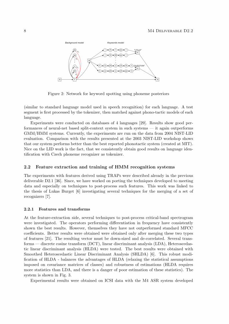
• Acoustic-based KWS. The models of keywords are assembled from 3-state phonemeHMMs. The confidence of the keyword is computed as a difference of 2 likelihoods:positive one from the last state of keyword-model and negative one from backgroundmodel (a phoneme-loop). The positive path is actually prepended with a phoneme-loop too, to allow for natural starts of keywords (Fig. 2). We have experimentedwith HMM/GMM models but also built a system using the phoneme or phoneme-state posteriors. The evaluation of FOM on 18 words from the ICSI corpus showsthat the neural-net split-context system systematically outperforms the GMM systems:CI-GMM: 47.8%, CD-GMM: 61.9%, split-context-3-state: 65.0%.

• KWS based on phoneme lattices. We are again using split-context system. Phonemelattices are generated by converting phoneme-posteriors into quasi-features and run-ning HTK decoder HVite. The parameters of lattice generation (branching factor andword-insertion penalty) are tuned using evaluation of lower-bound phoneme error rateon lattices. The keywords are detected using by a Viterbi algorithm with a simpleHMM accepting the arcs of the lattice instead of feature vectors. Several techniquesfor penalization of non-matching state/node pairs have been tested. In preliminaryexperiments, FOM of 58.3% was obtained.

As keyword spotting was identified as one of important components in a system for meetingbrowsing and real-time meeting processing, the work continues within the AMI project.

Language identification is another interesting application making use of phoneme rec-ognizer. Phoneme strings in training data are used to train an n–gram phono-tactic model


Figure 2: Network for keyword spotting using phoneme posteriors

(similar to standard language model used in speech recognition) for each language. A testsegment is first processed by the tokenizer, then matched against phono-tactic models of eachlanguage.

Experiments were conducted on databases of 4 languages [29]. Results show good per-formances of neural-net based split-context system in such systems — it again outperformsGMM/HMM systems. Currently, the experiments are run on the data from 2004 NIST-LIDevaluation. Comparison with the results presented at the 2003 NIST-LID workshop showsthat our system performs better than the best reported phonotactic system (created at MIT).Nice on the LID work is the fact, that we consistently obtain good results on language iden-tification with Czech phoneme recognizer as tokenizer.

2.2 Feature extraction and training of HMM recognition systems

The experiments with features derived using TRAPs were described already in the previousdeliverable D2.1 [36]. Since, we have worked on porting the techniques developed to meetingdata and especially on techniques to post-process such features. This work was linked tothe thesis of Lukas Burget [6] investigating several techniques for the merging of a set ofrecognizers [7].

2.2.1 Features and transforms

At the feature-extraction side, several techniques to post-process critical-band spectrogramwere investigated. The operators performing differentiation in frequency have consistentlyshown the best results. However, themselves they have not outperformed standard MFCCcoefficients. Better results were obtained were obtained only after merging these two typesof features [21]. The resulting vector must be down-sized and de-correlated. Several trans-forms — discrete cosine transform (DCT), linear discriminant analysis (LDA), Heteroscedas-tic linear discriminant analysis (HLDA) were tested. The best results were obtained withSmoothed Heteroscedastic Linear Discriminant Analysis (SHLDA) [6]. This robust modi-fication of HLDA - balances the advantages of HLDA (relaxing the statistical assumptionsimposed on covariance matrices of classes) and robustness of estimations (HLDA requiresmore statistics than LDA, and there is a danger of poor estimation of these statistics). Thesystem is shown in Fig. 3.

Experimental results were obtained on ICSI data with the M4 ASR system developed


bandprobabilityestimator

meanvariance

normalization

Hammingwindowing DCT

meanvariance

normalization


meanvariance

normalization


meanvariance

normalization


feature concatenation

HLDAdimensionality

reduction

Critical band spectrogram

BD G2

Modified critical band spectrogram

Bark filter−banks

Logarithm

FFT

Segmentation

bandprobabilityestimator

ME

RG

ER

decorrelation

Logarithm

PCA

TRAP processing

TRAP processing

Segmentation, FFT, Mel filter−bank, DCT

45TRAP

features

−1 −2 −1

01

−1 1 2 10 0 0

MFCC + delta + deltadelta 39 MFCC features

Figure 3: Speech recognition system combining TRAP-based and MFCC features with HLDAtransform.

jointly by University of Sheffield and VUT Brno. The improvement of combined TRAP-based and MFCC features over only MFCCs was almost 3% absolute.

2.2.2 SERest – new HMM training tool

For the experiments above (transforms, feature combination), we have started to develop atool for embedded training of HMMs compatible with the standard (model compatibility).This effort turned out to be widely accepted within the speech recognition community in M4and AMI. SERest currently features:

• Reference transcriptions can be given by lattices (easy to handle multiple pronuncia-tions, various noise models).

• Unsupervised model retraining (adaptation) on test data.

• Both Baum-Welch and Viterbi training are implemented.

• it is possible to use information about timing of labels (as in HTK tools HRest andHInit).

• Re-estimation of linear transforms (Maximum likelihood linear transform MLLT, lineardiscriminant analysis LDA, heteroscedastic linear discriminant analysis HLDA) withinthe training process.

• Discriminative training of models (Maximum mutual information) was recently finishedand is now extensively tested.

The tool is publicly available at:http://www.fit.vutbr.cz/speech/sw/stk.html.

2.3 Large Vocabulary Speech Recognition

A large vocabulary speech recognition (LVCSR) system was built using the publicly availableHTK toolkit [47] version 3.2. This version of HTK was not distributed with an efficient largevocabulary decoder. So in order to make an efficient LVCSR system the stack decoder calledDUcoder [46] was used also. Language models were created using the SRI language modellingtoolkit1 [43]. Due to various limitations in the software available to us it was found that the

1URL: http://www.speech.sri.com/projects/srilm/


best speed/accuracy trade-off was attained by using the DUcoder to generate n-best liststhat could be rescored by HTK’s HVite.

Word-internalcontext-dependent

triphone models

Cross-wordcontext-dependent

triphone models

Front end

MLLRadaptation

MLLRadaptation

Trigramlanguage model

Recognitionoutput

n-best list rescoringTime synchronous decoding

n-best list generationBest first decoding

Speech segments(e.g. from the M4 speech activity detector)

Figure 4: Dependencies between the components of the LVCSR system

Figure 4 illustrates dependencies between the components of the recogniser. The recog-niser empolyed two sets of context dependent triphone models: one set for word internaltriphone modelling and another for crossword modelling. Each set of models contained ap-proximately 4000 tied states with 16 Gaussians per state. These models were trained andadapted using the HTK toolkit. Adaptation was performed using maximum likelihood linearregression (MLLR). Recognition took two passes. In the first pass the DUcoder was usedwith the word-internal triphone models and the trigram language model to generate an n-bestlist. This limited the search space for the second stage in which HVite rescored the n-bestlist using the cross-word triphone models.

The trigram language models were created using Switchboard and ICSI meetings dataand interpolated together using weights 0.17 and 0.83 respectively to create an optimisedmodel.

The system was initially trained on the Switchboard database using transcriptions ob-tained from ISIP. It achieved a word error rate of 45.4% when tested on an hour of unseenSwitchboard data. For recognising meetings data the M4 speech activity detector was firstused to extract segments of the signals that correspond to the local speaker (thus eliminating


crosstalk between microphones). Adapting the Switchboard models to the ICSI meetingscorpus resulted in a word error rate of 46.1% when tested on meetings bmr001, bmr018 andbro018. However, when adapted and tested on M4 meetings this system achieved a signifi-cantly higher word error rate or 73.5%. In a comparative study conducted at ICSI using theSRI speech recogniser, a well established state-of-the-art system, a word error rate of 67.2%was achieved on the M4 meetings data.

One of the challenges of the M4 meetings data is the significant quantity of non-nativeEnglish speech. Better language modelling and pronunciation dictionaries may yield improvedresults. The largest single factor resulting in the high error rates on the M4 data is the lackof high quality hand transcriptions. Inaccurate transcriptions leads to poor adaptation andintroduces additional errors during the scoring process.

Follow-on work for a speech recognition system has continued as part of the AMI project(on which M4 partners are participating). The new system is built from scratch using thefull version of HTK that includes the efficient LVCSR decoder called HDecode. Amongstother features, the new recogniser incorporates better training algorithms, better speakeradaptation including maximum-a-posteriori adaptation and vocal tract length normalisation,wordlists generated from a significantly larger set of corpora, automatically generated pro-nunciation dictionaries that are manually corrected and better language models that are builtfrom over a billion words of normalised text. In all, this has resulted word error rates thatare significantly lower than the M4 recogniser.

Work on conversational telephone speech (CTS) was based on three corpora: Switchboard-I, CallHome English, and Switchboard cellular. Word level transcripts and audio segmenta-tions for training covering most of these corpora were obtained from Cambridge University(h5etrain03). Recognition experiments were conducted using the official 2001 NIST Hub5Eevaluation set. The 1998 and 2002 NIST Hub5E evaluation data were additionally used fortesting wordlists and language models. A word error rate of 32% was obtained for the CTStask.

The development of the meeting data recogniser naturally builds on the CTS recogniser.Acoustic models were bootstrapped from the CTS models with the ICSI meetings corpus andnew word lists, pronunciation dictionaries and language models were created. The word errorrates on the ICSI corpus part of the development and evaluation sets of the 2004 NIST RichTranscription meeting evaluations were 19.9% and 25.7% respectively.

2.4 Use of microphone arrays

2.4.1 Introduction

We have investigated the use of microphone arrays to acquire and recognise speech in meet-ings. Meetings pose several interesting problems for speech processing, as they consist ofmultiple competing speakers within a small space, typically around a table.

One of the problems that arises in meeting speech is that of multiple concurrent speakers.Overlapping speech may occur when someone attempts to take over the main discussion, whensomeone interjects a brief comment over the main speaker, or when a separate conversationtakes place in addition to the main discussion.

Due to their ability to provide hands-free acquisition and directional discrimination, mi-crophone arrays present a potential alternative to close-talking microphones in such an appli-cation. We first propose an appropriate microphone array geometry and improved processing


Tim

e A

lignm

ent

WienerPost-filterEstimation

x′1

x′2

x′N

x1

x2

xN

v1

v2

vN

w1

w2

wN

∑h

Figure 5: Filter-sum beamformer with post-filter

Microphone

Loudspeaker

PC

L1

L2L3

20cm Dia.

1.2m Diameter

10cm

Figure 6: Meeting Room Configuration

technique for this scenario, paying particular attention to speaker separation during possibleoverlap segments. Data collection of a small vocabulary speech recognition corpus (Num-bers) was performed in the meeting room for a single speaker, and several overlapping speechscenarios. In speech recognition experiments on the acquired database, the performance ofthe microphone array system is compared to that of a close-talking lapel microphone, and asingle table-top microphone.

2.4.2 Enhancement Technique

A block diagram of the microphone array processing system is shown in Figure 5. It includesa filter-sum beamformer followed by a post-filtering stage.

For the beamformer, we use the superdirective technique to calculate the channel filters wn

maximising the array gain, while maintaining a minimum constraint on the white noise gain.For the post-filter, we proposed an improvement on an existing technique by incorporatinglocalised competing speakers in the post-filter estimation procedure.

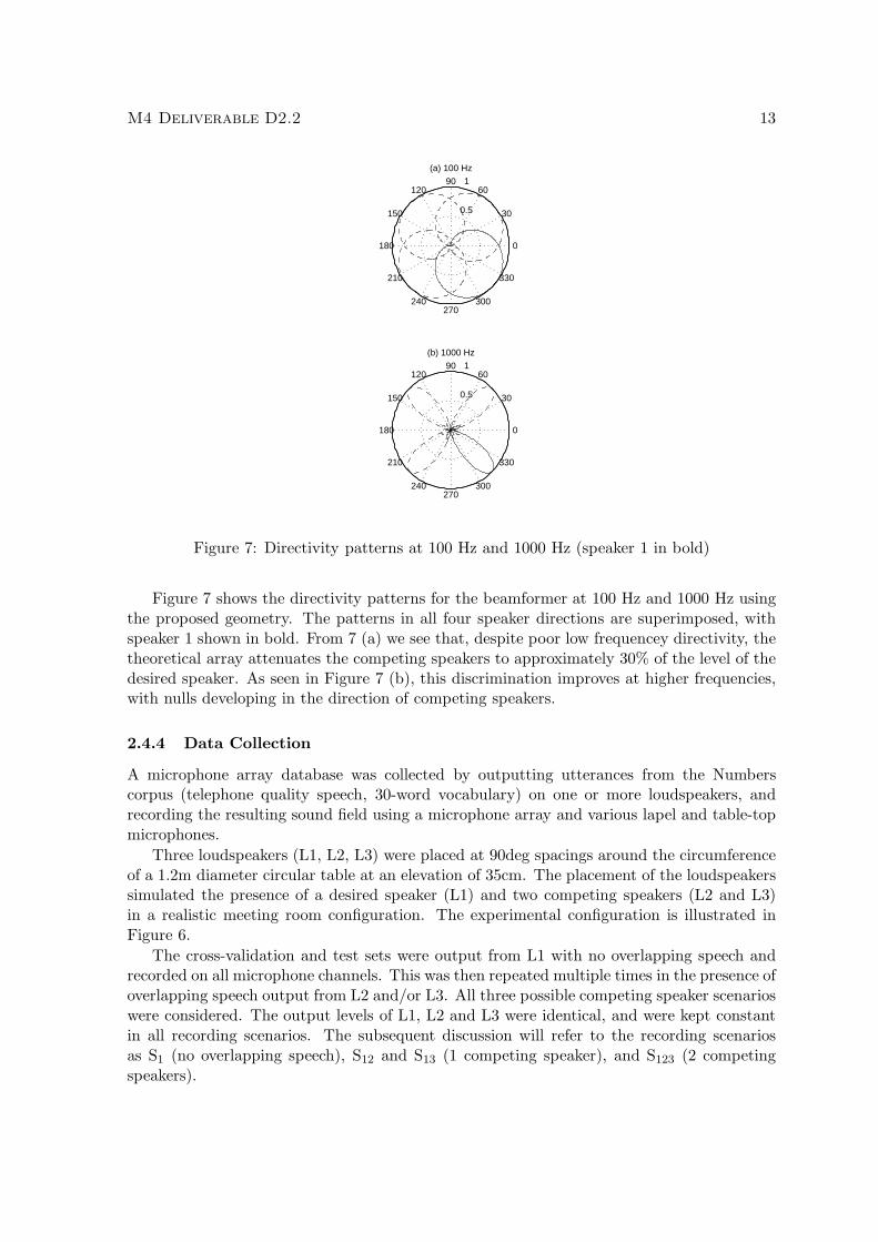
2.4.3 Array Geometry

In these experiments, we investigate a scenario where four people are equally spaced arounda small meeting table. To give uniform discrimination over all possible speaker locations, wepropose a circular array at the centre of the table. In particular, we use 8 equally spacedomnidirectional microphones, with diameter 20 cm. This configuration is shown in Figure 6.


0.5

1

30

210

60

240

90

270

120

300

150

330

180 0

(a) 100 Hz

0.5

1

30

210

60

240

90

270

120

300

150

330

180 0

(b) 1000 Hz

Figure 7: Directivity patterns at 100 Hz and 1000 Hz (speaker 1 in bold)

Figure 7 shows the directivity patterns for the beamformer at 100 Hz and 1000 Hz usingthe proposed geometry. The patterns in all four speaker directions are superimposed, withspeaker 1 shown in bold. From 7 (a) we see that, despite poor low frequencey directivity, thetheoretical array attenuates the competing speakers to approximately 30% of the level of thedesired speaker. As seen in Figure 7 (b), this discrimination improves at higher frequencies,with nulls developing in the direction of competing speakers.

2.4.4 Data Collection

A microphone array database was collected by outputting utterances from the Numberscorpus (telephone quality speech, 30-word vocabulary) on one or more loudspeakers, andrecording the resulting sound field using a microphone array and various lapel and table-topmicrophones.

Three loudspeakers (L1, L2, L3) were placed at 90deg spacings around the circumferenceof a 1.2m diameter circular table at an elevation of 35cm. The placement of the loudspeakerssimulated the presence of a desired speaker (L1) and two competing speakers (L2 and L3)in a realistic meeting room configuration. The experimental configuration is illustrated inFigure 6.

The cross-validation and test sets were output from L1 with no overlapping speech andrecorded on all microphone channels. This was then repeated multiple times in the presence ofoverlapping speech output from L2 and/or L3. All three possible competing speaker scenarioswere considered. The output levels of L1, L2 and L3 were identical, and were kept constantin all recording scenarios. The subsequent discussion will refer to the recording scenariosas S1 (no overlapping speech), S12 and S13 (1 competing speaker), and S123 (2 competingspeakers).


Scenario Lapel Centre ArrayS1 7.01 10.06 7.00S12 26.69 60.45 19.37S13 22.17 54.67 19.26S123 35.25 73.55 26.64

Table 3: Word error rate results

2.4.5 Experiments and Results

A baseline speech recognition system was trained using HTK on the clean training set fromthe original Numbers corpus. The system consisted of 80 tied-state triphone HMM’s with 3emitting states per triphone and 12 mixtures per state. 39-element feature vectors were used,comprising 13 MFCC’s (including the 0th cepstral coefficient) with their first and secondorder derivatives. The baseline system gave a WER of 6.32% using the clean test set fromthe original Numbers corpus.

Three recorded “channels” resulting from the data collection and microphone array pro-cessing were retained for speech recognition model adaptation and performance evaluation.These channels were:

• Centre tabletop microphone recording (Centre)

• Desired speaker (L1) lapel microphone recording (Lapel)

• Enhanced output of microphone array processing (Array)

MAP adaptation was performed on the baseline models using the cross-validation setfor each channel-scenario pair, and then the speech recognition performance of the adaptedmodels was assessed using the corresponding recorded test set. Table 3 shows the word errorrate (WER) results for all channel-scenario pairs.

From the S1 results, the WER’s for the Array and Lapel channels were the same, andcomparable to that of the baseline system. This shows that the recognition performanceof the table-top microphone array is equivalent to the close-talking lapel microphone in lownoise conditions. The WER for the centre microphone channel is slightly higher due to itsdistance from the desired speaker, and greater susceptibility to room reverberation.

The addition of a single competing speaker (S12 and S13) (resulting in approximately0dB SNR at the centre microphone location) had a severe effect on the WER for the centremicrophone channel. The lapel microphone channel performed substantially better due toits proximity to the desired speaker. This difference in WER was more pronounced when asecond competing speaker was introduced in S123 (resulting in approximately -3dB SNR atthe centre microphone location).

In all overlapping speech scenarios, the microphone array output gave better word recog-nition performance than both the centre and lapel microphone channels. These results areput in context when one considers that the individual microphones in the array were eachsubjected to essentially the same sound field as the centre microphone. The signal enhance-ment provided by the array processing overcame the lower SNR and increased reverberation


0 (20dB) 1 (0dB) 2 (−3dB)0

10

20

30

40

50

60

70

80

No. of Competing Speakers (with ~SNR at centre location)

WE

R (

%)

CentreLapel Array

Figure 8: WER results for different numbers of competing speakers

susceptibility, and improved recognition accuracy to a level that exceeded that of the close-talking lapel microphone.

Figure 8 illustrates the WER trends for each channel in scenarios with 0, 1 and 2 com-peting speakers. The values plotted for the single competing speaker case are the average ofthe S12 and S13 WER results shown in Table 3.

2.5 Localization and Speaker Segmentation

2.5.1 Introduction

In the framework of a meeting manager that would automatically detect, extract, transcribeand annotate speech, we studied microphone array-based speaker segmentation techniques.

Initial work [24, 26] showed that very accurate speaker segmentation can be obtainedbased on localization techniques, as compared to traditional single-channel acoustic features(LPCC). Speaker location information is typically extracted with a microphone array, thusalleviating the need for lapels to be worn by meeting participants. However, it does notprovide speaker identity information, therefore a clustering study was presented [1] thatcombines both location and acoustic informations.

The location-based segmentation approach addresses particularly well the case of sponta-neous multi-party speech, which contains many overlaps [40], that is when multiple speakerstalk at the same time. Further work [27] has successfully extended the approach to caseswhere the number and the locations of the speakers are not known a priori. Comparison withlapel-based speaker segmentation on real multi-party speech showed superior performancefor the location-based technique on overlaps, and comparable overall performance.

At this point, all work had been done based on single source localization techniques [9].However, exposure to real meeting data showed that apart from overlaps, there are many non-speech interferences such as beamer, laptop, fans, door slams, note-taking noises, body noises,etc. Thus we proposed to see the meeting room environment as a constantly multisourceenvironment.

The speaker segmentation task thus requires to detect (how many active sources?) andlocate (where are they?) multiple persons and noise sources active at the same time. Inexisting literature, the detection and localization problems are usually considered separately


test set FA PRC RCL F

Baseline: LPCC 88.3% 0.81 0.73 0.77Location, offline 99.5% 1.0 1.0 1.0Location, online 99.1% 0.99 0.99 0.99

Table 4: Supervised segmentation on data without overlapping speech. “FA” is frame accu-racy, “PRC” is precision, “RCL” is recall, and F = 2 × PRC × RCL/(PRC + RCL).

test set FA PRC RCL F

Location, offline 96.2% (88.1%) 0.93 0.93 0.93Location, online 95.4% (79.9%) 0.91 0.94 0.92

Table 5: Supervised segmentation on data with overlapping speech. Brack-ets show results calculated on actual overlap segments only. See Tab. 4for the meaning of FA, PRC, RCL and F .

and many results are presented on simulated data. On the contrary, we focussed on realdata recorded in a meeting room: the AV16.3 corpus [28] was recorded and annotated in3-D space. A sector-based approach was developed [25, 23] that discretizes the space arounda microphone array into volumes (sectors), and decides for each sector, whether it containsactive sources or not. This technique was developed in order to allow for existing localizationapproaches to locate precisely the source(s) within each sector separately. Speech segmenta-tion, separation and denoising can then be implemented based on the multisource locationestimates.

The remaining of this Section describes the AV16.3 corpus, and gives experimental resultsfor multisource localization and segmentation, including on real meeting data.

2.5.2 Supervised Location-Based Segmentation

“Supervised” means that the number and position of speakers are known a priori. Location-based features are extracted from the signals recorded by a 10-cm radius microphone array,centrally located on a meeting room table. These features are then filtered into a speech/non-speech segmentation for each person, that allows overlapping speech segments. An offline,HMM-based technique [24] as well as online techniques [26] were proposed and tested onseveral 4-speaker cases, and compared with a LPCC-based single channel baseline. Resultsreported in Tab. 4 and 5 show that the proposed techniques are very accurate on data with upto two simultaneous speakers. A major improvement is seen compared to the single channelbaseline.

2.5.3 Data Collection: the AV16.3 corpus

A corpus of real audio-visual data for speaker localization and tracking was designed, recordedand annotated in terms of 3-D speaker location [28]. “16.3” means 16 microphones and3 cameras. Many different cases of overlapped speech, moving and static speakers, free andconstrained scenarios were recorded. The idea is to have specific test cases recorded in a


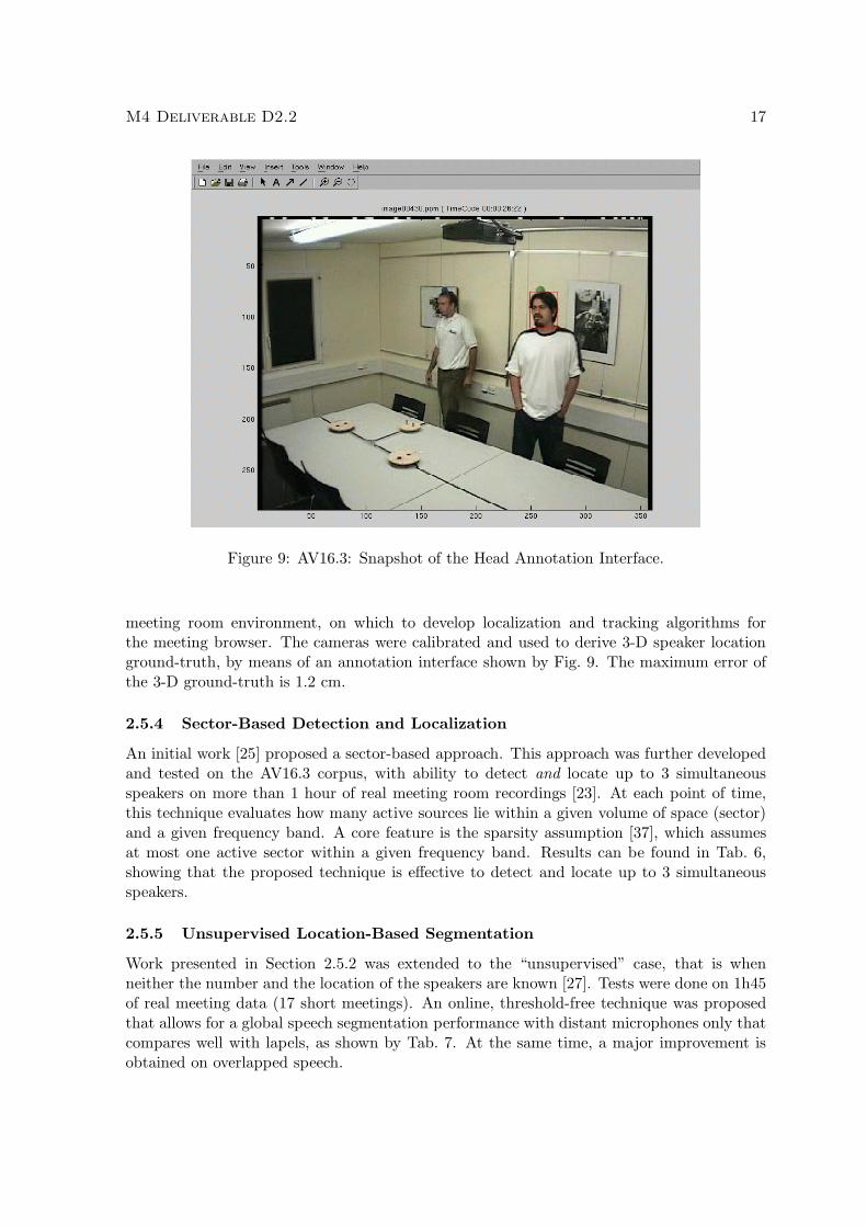
Figure 9: AV16.3: Snapshot of the Head Annotation Interface.

meeting room environment, on which to develop localization and tracking algorithms forthe meeting browser. The cameras were calibrated and used to derive 3-D speaker locationground-truth, by means of an annotation interface shown by Fig. 9. The maximum error ofthe 3-D ground-truth is 1.2 cm.

2.5.4 Sector-Based Detection and Localization

An initial work [25] proposed a sector-based approach. This approach was further developedand tested on the AV16.3 corpus, with ability to detect and locate up to 3 simultaneousspeakers on more than 1 hour of real meeting room recordings [23]. At each point of time,this technique evaluates how many active sources lie within a given volume of space (sector)and a given frequency band. A core feature is the sparsity assumption [37], which assumesat most one active sector within a given frequency band. Results can be found in Tab. 6,showing that the proposed technique is effective to detect and locate up to 3 simultaneousspeakers.

2.5.5 Unsupervised Location-Based Segmentation

Work presented in Section 2.5.2 was extended to the “unsupervised” case, that is whenneither the number and the location of the speakers are known [27]. Tests were done on 1h45of real meeting data (17 short meetings). An online, threshold-free technique was proposedthat allows for a global speech segmentation performance with distant microphones only thatcompares well with lapels, as shown by Tab. 7. At the same time, a major improvement isobtained on overlapped speech.


Loudspeakers HumansMetric Target Result Target Result

FAR 0.5% 0.5% 0.5% 3.0%N2 2.0 1.9 1.3 1.3N3 3.0 2.5 2.0 1.6

Table 6: Sector-based detection and localization results. FAR is the False Alarm Rate, N2

(resp. N3) is the average number of speakers correctly detected when 2 (resp. 3) speakersare simultaneously active. N2 and N3 targets are lower for humans because silences betweenwords are included in the ground-truth segmentation.

Proposed Lapel baselinePRC 0.80 ( 0.55 ) 0.84 ( 0.47 )RCL 0.95 ( 0.85 ) 0.93 ( 0.66 )F 0.87 ( 0.67 ) 0.89 ( 0.55 )

Table 7: Unsupervised segmentation on 17 short meetings. The proposed approach usesdistant microphones only. Results on overlaps only are indicated in brackets. See Tab. 4 forthe meaning of FA, PRC, RCL and F .

On the tracking side, this approach was successfully extended to detect trajectory cross-ings. This work was presented at the NIST RT-04 workshop.

2.6 Localization and tracking of multiple speakers simultaneously

2.6.1 Introduction

A method has been being developed for localizing and tracking multiple sources simultane-ously, using an array of microphones. With the knowledge about the locations of the sources,the speech signals of the multiple sources can be separated with a suppression in order of25 dB. Since a patent application on this topic is being submitted, technical details of themethod are still confidential.

2.6.2 Numerical simulations

The method was verified on synthetic data. An acoustic finite difference simulation wasmade for a room with three sources. The reflections and diffraction due to the walls andthe furniture in the room were included in the finite difference simulation. The processedsimulated data on the receiver array showed that 25 dB suppression between the multiplesources is possible.

2.6.3 Experiments

In the next phase the method was verified in a live experiment. The experiment consistedof 3 speakers centered around a table, while they were in constant discussion moving aroundthe table, even changing positions. The experimental results showed an accurate localization


and tracking of the sources with an accuracy in the order of 5 cm. The position change of twospeaking persons was also accurately tracked. The speech signals belonging to the speakerswere separated with a suppression between 20 - 30 dB, depending on the distance betweenthe speakers and the length of the speech. Complete words or sentences performed betterthan short vowel sounds.

Improvements can be made if the data on the receivers is recorded with a better signal tonoise ratio. At the moment a lab is equipped at TNO for dedicated and controlled experimentswith the microphone array, in order to improve the method.

2.6.4 Conclusion

The method showed good results in localizing and tracking multiple sources simultaneously,separating the speech signal of the multiple sources with a suppression in the order of 25 dB.



3 Video processing

The main task of the video processing is to provide basic information about the location of aperson and to extract features that can be used for low level gesture recognition, which willbe basically necessary for the recognition of (high level) group actions. Therefore we havedeveloped an architecture consisting of several basic modules, comprising different detectorsfor faces/heads, an algorithm to track the detected persons as well as a feature extractionand classifier module.

Localizing and tracking people play important roles in meeting analysis. As a data source,meetings recorded in multi-sensor rooms consist of unedited streams of audio and video,captured with multiple cameras and microphones covering participants and workspace areas.In such setups, tracking is useful to determine the number and location of participants, toprovide accumulated information for person identification, to select a fixed camera or to steera motorized one as part of a visualization or production model, to enhance the audio streamfor speech recognition using microphone arrays, and to provide cues for detection of location-based events. In all of these cases, the availability of multiple views and modalities representsan advantage.

Tracking people and their activity is also relevant for higher-level multimodal tasks thatrelate to the communicative goal of meetings. Experimental evidence in social psychology hashighlighted the role of non-verbal behavior (e.g. gaze and facial expressions) in interactions[32], and the power of speaker turn patterns to capture information about the behavior ofa group and its members [30, 32]. Identifying such multimodal behaviors requires reliablepeople tracking.

In the M4 project, we developed algorithms to track people in meetings for several of thetasks described above, using a consistent Bayesian framework, namely sequential Monte Carlo(SMC) methods or particle filters (PF). SMC methods approximate the Bayesian solution tothe tracking problem using sampling techniques, and have gained popularity in recent yearsto deal with non-linear and non-Gaussian state-space models, due to their versatility, ease ofimplementation, and success in challenging applications. As part of the project, we developedPFs to track multiple interacting people, with occlusion as the typical problem in meetingrooms, to track location and head pose, as a surrogate for gaze, and to track location andspeaking activity using audio-visual data. Overall, our work in tracking can be seen as abuilding block towards building probablistic models of multimodal human interaction.

3.1 Mobile USB 2.0 Camera

3.1.1 Hardware

To simplify the installation and to reduce costs, the EPFL has proposed a miniature pan/tiltcamera for the M4 project. This camera should provide a easy-to-use data collection.

Camera history:

• Pal camera (ANALOG)

– Separated alimentation (12V)

– Separated motors control via RS232

– Analogical video signal (PAL)


• USB 1.1 camera (DIGITAL)

– All in one alimentation / motors control / digital video signal (VGA 640x480)through one USB cable

• USB 2.0 camera (DIGITAL)

– All in one alimentation / motors control / digital video signal (SXGA 1280x1024)through one USB cable

The installation process of the analog camera – with its three cables – was too heavy. Wethus decided to transfer the whole technology into a more compact and digital version of thecamera. A USB interface has been chosen because it is a widely used system.

Many adaptations were then necessary:

• The camera need in terms of electrical consumption has been adapted to the USBspecification,

• A USB hub has been mounted on the PCB so video data and control order could transitin the same cable,

• The emulation of the RS232 protocol has been possible via a virtual com port (FTDI).

A demonstrator has been achieved and successfully tested. The next step was to adaptthe electronics of the Pan/Tilt camera itself to obtain a usable prototype. The first digitalcamera was using USB 1.1 and motion jpeg compression; this technology, however, createsimage artefacts.

Our final work has been to migrate to USB 2.0 version. Compared to USB 1.1, USB 2.0allows a higher bit rate (up to 480 Mb/s vs. 12 Mb/s) and also less computational power tohandle video stream due to absence of compression on the camera side and decompressionon the PC side.

The mechanical part of the camera (shown on the figure here after) was difficult to handle.Most problems have been solved but the production of these parts is not yet optimum. Thusit is currently still difficult to get parts from manufacturers.

Today, the USB 2.0 Pan/Tilt camera is based on a colour sensor from Omnivision Tech-nologies, the OV9620, which is a specially-designed, high-performance 1.3 mega-pixel single-chip CMOS image sensor for digital still image and video camera products. It incorporates a1280 x 1024 (SXGA) image array and an on-chip 10-bit A/D converter capable of operatingat up to 30 frames per second (fps) with full resolution. Proprietary sensor technology utilizesadvanced algorithms to cancel Fixed Pattern Noise (FPN), eliminate smearing, and drasti-cally reduce blooming. The control registers allow for flexible control of timing, polarity, andchip operation.

The sensor features are regrouped here after:

• Optical Black Level Calibration

• Video or Snapshot Operations

• Programmable/Auto Exposure andGain Control

• Programmable/Auto White BalanceControl

• Horizontal & Vertical Sub-sampling (4:2and 4:2)


Figure 10: EPFL USB 2.0 Camera prototype

• Flexible Frame Rate Control

• On-Chip Defect Column and Pixel Cor-rection

• On-Chip R/G/B Channel and Lumi-nance Average Counter

• Internal/External Synchronization

• Power on Reset and Power Down Mode

• Array Format Total: 1312 H × 1036 V

• Active: 1280 H × 1024 V

• Image Area Total: 6.82 × 5.39mm2

• Active: 6.66 × 5.32mm2

• Pixel Size 5.2µm × 5.2µm

• Optical Format 1/2′′

• Color Mosaic RGB Bayer Pattern

• Max Frame Rate 30 fps at 1280 × 1024

• 120 fps at 640 × 480


• Electronics Exposure 1.8µs to 1/30s

• Scan Mode Progressive

• Output 10 Bit Digital

• Min. Illumination (3000 K)

However, these values (in particular the frame rate), even if specified by the manufacturer,cannot be fully exploited because of the following points:

1. USB 2.0 capabilities: in theory, the maximum frame rate that could be achieved througha USB 2.0 connection should be (that is, if the whole transfer rate could be used,encapsulation excepted):

Resolution Frame rate640 × 480 50 fps

1280 × 1024 12 fps

Table 8: Maximum resolution supproted by USB 2.0 bandwidth

2. The drivers used to capture video streams come from Omnivision. These drivers arestill beta versions and some stability problems have been encountered. Omnivisiondoes not seem to work on new drivers, so we should concentrate on creating our own.Moreover, the efficiency of these drivers are not optimum, as shown in the followingtable:

Resolution Frame rate640 × 480 20 fps

1280 × 1024 5 fps

Table 9: Maximum resolution supproted by Omnivision drivers

We have also discovered a recent dysfunction that disallows the SXGA format to be usedon the Pan Tilt camera version. That problem comes from our USB hub and has the effectof displaying images as black screens. For now, VGA format is the only workable one.

Last point, the pan & tilt functions are now well controlled and easy to use.

3.1.2 Software

In parallel, application-programming interfaces (API) have been developed to facilitate imageacquisition, face tracking and camera positioning. These API are generic and should workfor different environments such as Windows and Linux. For that development, open-sourcelibraries and software tools have been experienced. Concerning video capture, OpenCV(Open Computer Vision Library) working both under Windows and Linux, and for imageprocessing, OpenCV jointly to IPL (Image Processing library) have been employed. Thesetools work under both Windows and Linux. These libraries are free and are optimized forMMX.

In this frame, an automatic cameraman algorithm based on colour tracking has beendeveloped and is currently used to pilot the USB 2.0 camera. A typical result can be seen infigure 12.


Imageanalysis

regulatorMotorized

base

User(target)

Image

Camera

Image centerPosition

Face positionin image

Figure 11: Tracking system

Figure 12: Face detection process - color based algorithm


3.2 Sequential Monte Carlo framework

The Bayesian formulation of the tracking problem is well known. Denoting by Xt the hiddenstate representing the object configuration at time t, and by Yt the observation extracted fromthe image, the filtering distribution p(Xt|Y1:t) of Xt given all the observations Y1:t = (Y1 . . . Yt)up to the current time can be recursively computed by [10]:

p(Xt|Y1:t) = Z−1p(Yt|Xt) ×∫

Xt−1

p(Xt|Xt−1)p(Xt−1|Y1:t−1)dXt−1 (1)

where Z is a normalizing constant. A PF is a numerical approximation to the above recur-sion in the case of non-linear and non-Gaussian models. The basic idea behind PF consistsof representing the filtering distribution using a weighted set of samples Xn

t , wnt Ns

n=1, andupdating this representation as new data arrives. With this representation, Eq. 1 can beapproximated by :

p(Xt|Y1:t) ≈ Z−1p(Yt|Xt)Ns∑

n=1

wnt−1p(Xt|Xn

t−1) (2)

using importance sampling. Given the particle set at the previous time step Xnt−1, w

nt−1,

configurations at the current time step are drawn from a proposal distribution q(Xt) =∑n wn

t−1p(Xt|Xnt−1). The weights are then computed as wn

t ∝ p(Yt|Xnt ).

Four elements are important in defining a PF:1. The state space. We use mixed-spaces, where the state is the conjunction of contin-

uous variables specifying the spatial object configuration (e.g. position, scale) and discretevariables labeling the object state (e.g. whether a person is occluded or not).

2. The dynamical model p(Xt|Xt−1) defines the temporal evolution of the state.3. The observation likelihood p(Yt|Xt) measures the adequacy between the observation

and the state.4. The sampling mechanism places new samples as close as possible to regions of high

likelihood.These elements, along with specific issues and proposed solutions, will be described in

each of the following three sections.

3.3 Face detection

Within the scope of M4 we have implemented and evaluated two discriminative techniquesfor the detection of features indicating the appearance of humans in the image.The first approach, heavily based on the neural network (NN) proposed by H. Rowley [38]et al., uses the face as an obvious feature and provides - if the face is visible in the image- quite robust results. For this method an artificial neural network has to be trained witha sufficient number of positive and negative examples of faces showing different angles forthe line of sight (i.e. not only frontal and upright faces). In order to reduce the influence ofthe lightning conditions two further preprocessing steps, lightning correction and histogramequalization, are applied to the training samples. The gray level intensities obtained afterthe histogram equalization are directly fed to the input layer (20 × 20 pixel) of the NN. Thearchitecture of the NN is chosen to be a multiple layer perceptron (MLP), where the hiddenlayer consists of 26 hidden units representing so called receptive fields, which can describespecial localized features, such as mouth, nose or eyes. Finally the output neuron produces


an estimate for the presence of a face in the image sample (value greater than zero) or absenceof a face (value lower or equal to zero).In order to detect faces in an image, 20× 20 pixel sub-images are shifted and scaled over thewhole image, preprocessed by lightning correction and histogram equalization and finally fedto the NN as shown in Figure 13. In this way we obtain an output for each sub-image from theNN, which can be used to compute a likelihood for a face in the respective sub-image. Since

Figure 13: Overview over the NN based face-finding module

the face of a person is not always visible although the person itself might be visible in theimage, another approach uses not the face as feature for the detection process, but the shapeof the head, which can be approximated by an ellipse, which has a ratio of major to minoraxis of about 1.2. The procedure to detect heads is mainly as follows: At first the gradientimage is computed and a standard ellipse, i.e. an ellipse with a certain length of the majoraxis, is shifted and scaled over all possible locations on the image, resulting in sub-imagesequivalent to those described above. In every sub-image, the dot product between the unitvector of the ellipse, calculated at discrete sample points, and the gradient at that imageposition is computed. In Figure 14 this procedure is visualized exemplarily for eight samplepoints. In order to allow some noise in the image data, the calculation of the dot productdescribed above is done for all pixel along the normal vector within a certain distance aroundthe ellipse sample point (cf. straight lines in Figure 14). Thus we obtain a probability forthe presence of a head at this position by summing up the best result for the dot productat each sample point. Now high scores mean a good interpretation of the image data by theelliptical structure and thus indicate a probable presence of a head at this position.Although both methods show reliable results, the amount of computations dramatically riseswith the dimension of the image. For this reason an algorithm has been developed based ona low level indicator like the color information to reduce the amount of sub-images beforethese are evaluated by one of the presented approaches. All sub-images, which do not haveat least a certain number of skin colored pixels, are discarded. To determine skin coloredpixels, the RGB-values are transformed into the rg-chroma space. Now the first approachis to define a skin color locus as done by M. Storring and his colleagues. All skin coloredpixels are determined by the area depicted in Figure 15. Another approach uses the idea todescribe the skin color distribution in the rg-chroma by a Gaussian Mixture Model (GMM).The parameters of the GMM have been computed from a training distribution, that has been


Figure 14: Measurement of the head likelihood based on the thresholded gradient image

Figure 15: Location of skin color pixels in the red-green-chroma space

built by manually picking around 5000 skin colored pixels. Both approaches provide goodresults at least for our indoor scenarios and thus enable a reliable reduction of importantsub-images, which have to be evaluated furthermore.

3.4 Person Tracking

A further improvement could be achieved by the integration of the face/head detection algo-rithm into a particle filter framework presented by Isard [16, 17] et al. The basic idea of thisapproach is to produce hypotheses at different locations in the image, which should describethe probability for the appearance of a face/head. In this way a discrete representation ofthe probability distribution is generated and each hypothesis now can be evaluated by themeasurement described in section 3.3. Due to the particle filtering framework hypotheseswill be taken over to the next time step by sampling corresponding to their probability,i.e.hypotheses with a high probability will be chosen more likely, and thus hypotheses will finallyconcentrate on the true position of the face/head.In order to avoid this behavior and to track several humans simultaneously, we have expandedthis approach for multiple person tracking by adding another layer to the particle filter. Thislayer is mainly responsible for the distribution of the hypotheses in the image, so that a con-


centration only on one position can be prevented. In Figure 16 a series of frames is shown,where two persons in a meeting are simultaneously tracked. The position of the heads, whichis determined by the algorithm, is marked by the ellipses.

Figure 16: Example frames for a typical tracking result

3.5 Person tracking using omnidirectional view

The main purpose of the method is monitoring of gestures and movement of people in ameeting room. Such task traditionally uses several video cameras. The disadvantage ofhaving to use several cameras can be resolved by using one omnidirectional view system.The system is based on standard or high resolution video camera equipped hyperbolic mirrorand allows capturing a large portion of the space angle - e.g. 110 × 360 degrees. Two optionsexist to set-up such system (cf. [44]). Mirror can be on above or below the camera. The mainfunctional difference is in the location of the area with highest resolution, because resolutionis decreasing from the edge to the centre of the mirror.

3.5.1 Tranformation omnidirectional view

An image obtained using the hyperbolic mirror can be transformed into a standard perspec-tive image. A simple transformation that presumes linear pixel distribution along the radiusdirection can be used. The coordinates of the panoramic view are Px and Py. These coor-dinates must be transformed into the omnidirectional image. The real world elements areprojected on a cylinder whose radius is equal to d. The axis of the cylinder is identical tothe mirror and camera axis. The horizontal size of the panoramic view is a perimeter of thecylinder (width = 2πd). The coordinates of the video camera image XM are the following:

xM = (d − Py) cosα + CenterX (3)

yM = (d − Py) sinα + CenterY (4)

with angle α = Pxd .


The calculated pixels in the camera image do not correspond ”one to one” to the pixelson the projected image so some subpixel anti-aliasing methods should be used.

Figure 17: Transformation into panoramic view

As the perspective projection ”center pf projection” is in most cases too close to theobserved objects, the images appear ”deformed”. It is possible to ”visually compensate” thisdeformation, if we know the properties of the objects. The geometrical corrections are basedon user-provided input information. The user identifies three points in the image which defineborder of the circle area. From these three points are computed parameters of the circle ascenter and radius. We define two curves between which we are making pixel interpolation(see Fig. 18).

Figure 18: Removing distortions

This transformation solves deformations in the vertical direction. Another deformationoccurs because of the image is cylindrically projected. This deformation can be transformedby the help of the perspective projection the cylindrical image into the plane. We can do this,because the properties of this projection are known from the room set-up. The method whichwe used is simple weighted interpolation for removing the non-uniformity in the horizontal


direction. These transformations are made because the algorithm for detection need non-deformed image of the face.

3.5.2 Hand and face tracking

Human face detection, gesture recognition, and other applications for tracking of humansare based on the assumption that the areas of human skin are already detected and located.Color is the key feature for hands and face detection. The color-based methods are mostcommonly used for this task and their main advantage is low computational cost. On anegative side, it is only a partial method because of its low reliability.

Figure 19: Skin color detection

For distinguishing colors between the human skin and other image regions, the distributionof skin color must be known a priori within the normalized color space. Therefore, we usednormalized rg-color space that provides good solution to the problem of varying brightness.Normalized rg-color is computed from RGB values:

r =R

R + G + Band g =

G

R + G + B(5)

Various face color pixels are picked manually and then color class Ωk is computed [18].The color class Ωk is determined by its mean vector µk and the covariance matrix Kk by itsdistribution. We need to compute probability of each pixel in the image by this equation:

p (c|Ωk) =1

2π√

detKkexp

(−1

2(c − µk)

T K−1k (c − µk)

)(6)

The use of Gaussian mixture in an illumination-normalized color space produced compa-rable results to a single Gaussian model [20]. Often the results of skin color detection eithercontain noise, or many colored objects create considerable clutter in skin probability imageand thus make skin regions not so clearly distinguishable. For this reason, the morphologicaloperator-based (dilatation and then erosion) was applied. The spatially separated groupsof skin pixels are treated as separate objects. Each object can be described by the ellipse.Parameters are computed from object pixel positions by using ellipse fitting algorithm.


Figure 20: Skin detection in transformed image

The omni-directional system has different properties compared to a standard perspectivecamera. It is necessary to adapt standard methods for finding hands and faces for usage inomni-directional images. Our next goal is to analyze properties of omni-directional images,which includes the color statistics depending on different lighting conditions and mirror ge-ometry. The human detected parts are then tracked. The location prediction method is usedfor this task. Information about motion in previous frames serves for computation of thevelocity and acceleration of tracked object.

Figure 21: Object correspondence

Finally, a GWN face detector is used for detection of the human faces in these areas andfor recognition of a specific person.

The face detector must answer the question if there is a face or not in the defined iamgeregion. Additionally it determines the exact face position. The key part of our face detectionalgorithm is the human face representation method. Discrete face templates are representedby linear combinations of wavelet functions (Gabor Wavelet Networks). Using this represen-tation, an effective face detection method is achieved, which is robust to illumination changesand deformations of the face image. The detection algorithm we used could be classified as afeature-based as well as template-based approach. Image features, such as edges and image


Figure 22: Head orientation detection

function variations, are modeled by wavelets. Because the wavelet position is known, theinformation about overall face geometry is presented, too. The wavelet parameters, such asrotation and scale, and relative wavelet positions describe the face geometry. This waveletrepresentation can be used for sparse and efficient template matching. During the face detec-tor training phase a gallery of GWN face templates is obtained. Then the gallery is used forthe detection. Detector attempts to find an affine transformation of gallery face template.The transformation which best fits the tested region is treated the best one. In other words, itprovides the best face alignment. The most suitable GWN template represents the detectedface and the transformation gives us the exact face position. If there is no suitable template,the detector returns negative answer - the region doesn’t contain the human face.

3.5.3 Mouth localization in low resolution image

Within the scope of M4, a mouth localization problem has been researched for the lowresolution images. Although the image itself had high resolution, the face images form alwaysonly a small portion of the image. From the original image, the head images have beenobtained using head detection algorithms. Color and convolution filtering approaches havebeen used to obtain the probability of the pixels being part of the mouth region.

First, the saturation and inverted logarithmic hue is obtained. Both images are thenprocessed to obtain the lip features representation. This information can be used for detectingpixels with highest lip color score. Very small parts, considered as noise or too small to belips are removed. Finally, the mouth map image is created, where region represents mouthand lips of target image. The lips region shape is parameterized and the parameters are usedas an additional input feature for the sound processing.


Figure 23: Main steps in mouth detection process

3.6 Tracking multiple people

The long-term, reliable tracking of multiple people in meetings is a challenging task. Meetingrooms pose a number of issues for visual tracking including occlusion, clutter, variation ofillumination, and variation of appearance arising from changing pose. On the other hand,multi-sensor meeting rooms offer some unique advantages that ease the task of tracking.These can include constraints on the working space and group dynamics, and redundanciesin video data from cameras with overlapping FOVs.

We define a joint multi-object state space, which constitutes a rigorous implementationof the problem. The state Xt contains the configuration for every person in the scene Xt =(x1,t, ..., xM,t), where M denotes the number of people, and xi,t contains translation andscaling parameters for person i.

Tracking a significant number of objects in a joint-object framework becomes increasinglydifficult as adding new objects to the scene increases the search space exponentially. A sam-pling strategy known as Partitioned Sampling (PS) helps reduce the dimensionality problemby handling one object at a time, but introduces problems with bias and impoverishment ofthe particle representation, dependent on the object ordering. We propose sampling usingDistributed Partitioned Sampling (DPS), which redefines the distribution as a mixture modelcomposed of subsets of particles, each of which performs PS in a different ordering [41]. InDPS, we re-express Eq. 1 as

p(Xt|Y1:t) =C∑

c=1

πc,t pc(Xt|Y1:t) (7)

where pc is a mixture component and c = 1, ..., C is the subset index. PS is performedusing a different ordering for each subset to fairly distribute the bias and impoverishmenteffects between each object. The subsets are then reassembled and evaluated normally.

The observation model used in this work consisted of 8-bin color-space (HS) histograms


seq PF PS PS PS DPS(1 → 2 → 3) (2 → 3 → 1) (3 → 1 → 2)

1 32 18 40 34 1002 10 0 12 0 78

Table 10: Tracking success rate for an occluded object for different sampling methods on two meetingroom data sequences. For PS, the numbers correspond to different object orderings.

with spatial components. The resulting multi-dimensional histogram consists of a concate-nation of 2-D HS histograms, each built from pixels taken from different areas of the head(eyes, mouth, hair, etc) according to a template. The observation likelihood is defined asp(Yt|Xt) =

∏i p(Yi,t|xi,t), where Yi,t is the image region enclosed by xi,t, and each object

likelihood is defined as p(Yi,t|xi,t) ∝ e−λd2i (Yi,t) where λ is a hyper-parameter and di(Yi,t) is

the distance based on the Bhattacharyya coefficient between the observation Yi,t and thespecific object template histogram.

Head tracking experiments were conducted in the meeting room to test the ability ofDPS to overcome impoverishment problems associated with PS. Specifically, DPS and PSwere tested for their ability to recover from occlusion (impoverishment hinders this ability)over 50 runs per method, to account for the stochastic nature of the tracker, with NS = 200particles. Performance is measured by the success rate (SR), the percentage of successful runs(a successful run occurs when the tracking estimate overlaps the ground truth throughoutthe entire sequence). As seen in Table 10, DPS signficantly outperformed both a simplemulti-object PF (denoted by PF) and a PS tracker. Some results can be seen in Fig. 24.

Figure 24: Tracking multiple heads through occlusion with DPS sampling in the multi-sensor meetingroom.

3.7 Tracking head pose

Head pose estimation is often used as a first step for other higher level tasks such as facialexpression recognition or gaze direction estimation. In meetings, head pose can be reasonablyused as a proxy for gaze (which usually calls for close views), and can thus be useful for de-termination of visual focus-of-attention and addressees in conversations. Most of the existingwork for head tracking and pose estimation defines the task as two sequential and separateproblems: the head is tracked, its location is extracted, and the head pose is estimated fromthe head location. As a consequence, the estimated head pose totally depends on the trackingaccuracy. This formulation misses the fact that knowledge about head pose could be used toimprove head modeling and thus improve tracking accuracy.


We couple head tracking and pose estimation using a mixed-state PF [2]. The stateXt = (xt, lt) is a mixed variable. The continuous variable x = (T, s) specifies the headlocation and scale. The discrete variable l specifies an element of the head pose exemplarsset. The pose at given time is obtained by marginalizing over the spatial configuration partof the state. In the following paragraph, we describe the head pose models, the dynamicalmodel, and the observation model.

Head pose exemplars are learned using the PIE database. A total of Nθ head poses aredefined by a pan angle ranging from -90 to 90 degrees discretized with 22.5-degree steps.For each head pose θ, Gaussian and Gabor features are extracted from training images,concatenated into a single feature vector, and clustered with K-means into Lθ clusters eθ

l =(eθ

l,j), l ∈ Lθ, |Lθ| = Lθ. The cluster centers are taken to be the head pose exemplars. Thenumber of elements of each cluster are used to define prior distributions πθ

l , and the diagonalcovariance matrix of the features σθ

l = diag((σθl,j)) is used to define pose probability models.

The pose of an head image is estimated by extracting its feature vector Y = (Yj), and findingthe pose MAP estimate by p(Y |θ) =

∑l∈Lθ

πθl p(Y |l), with

p(Y |l) =∏j

1σθ

l,j

max(exp−12

(Yj − eθ

l,j

σθl,j

)2

, T ) (8)

where T is a bound introduced to tolerate modeling errors.

The dynamical model is a second order autoregressive process p(Xt|Xt−1,Xt−2). Assum-ing that the two components xt and lt are independent, and that head pose depends only onthe previous pose give, the dynamics factorize as p(xt|xt−1, xt−2)p(lt|lt−1).

Finally, the observations are obtained by extracting the features Y (x) from the im-age region specified by the spatial configuration x. The observation likelihood is given byp(Yt|Xt) = pT (Yt(xt)|lt), with pT defined in Eq. 8.

Head pose estimation was tested on PIE database. The best result was obtained with twoexemplars per pose, with a recognition rate of 94.8% while the state-of-the-art obtains around90%. More details about evaluation can be found in [2]. The joint tracking algorithm wasalso tested on video sequences from our meeting room. An example with NS = 100 particlesis shown in Fig. 25. Tracking and head pose estimation are visually quite satisfactory.However, in view of the limitations of visual evaluation, and the inaccuracy obtained bymanually labeling head pose in real videos, we have recently recorded a set of meetingswith four participants, with head pose ground truth produced by a flock-of-birds device. Anobjective evaluation of our algorithm is in process.

3.8 Person action recognition

For the recognizer now features have to be extracted, which are able to describe these actionssufficiently and which are easy to compute at the same time. As shown in [49], global motionfeatures calculated on difference images of successive frames are capable of representing ac-tions occurring in such meeting scenarios. With these features we have now a 7-dimensional


Figure 25: Joint tracking and head pose estimation in meeting room. The green box and red arrowspecify the estimated head location and head pose, respectively. The red circle gives informationabout the pose value; its radius corresponds to 90 degrees. The participants are looking at the roomentrance.

stream consisting of

m(t) = [mx(t),my(t)] (center of mass),∆m(t) = [∆mx(t),∆my(t)] (change of the center),

σ(t) = [σx(t), σy(t)] (variance of motion) andi(t) (intensity of motion).

In order to examine only relevant features, i.e. differences in two successive frames causedby one person, a so called action region is defined around the located face/head position,which can be obtained by the tracking procedure (cf. section 3.3 and 3.4). After the featureextraction the feature stream was segmented and labeled manually for all of the meetingsrecorded within the scope of M4. Features extracted in the first half of the complete meetingrecordings were used for the training of six different Hidden Markov Models (pointing, writing,standing up, sitting down, nodding, shaking head), while the other half of the features wasused to evaluate the recognizer. In our experiments we have examined HMMs with differentcombinations of states and mixtures, but the best recognition rate of about 82% (testingevery class against each other) we have achieved for six states and three mixtures.In a further experiment [48] we have examined the influence of occlusions on the featuresand tried to compensate them by a special structure using Kalman filters. Since there wereno occlusions in the recorded meetings, we had to simulate artificial occlusion by applyingblack boxes to our action regions as depicted in Figure 26. Experiments with these artificial

(a) (b) (c) (d)

Figure 26: Different types of artificial occlusions


Kalman1

Kalman2

Kalman6

HMM1

HMM2

HMM6

m

a

xKalman

HMM1

HMM2

HMM6

m

a

x

Figure 27: System overview: action specific filter system on the left side, global filter systemon the right side

occluded feature streams have been run on two systems (Table 27). The first one uses oneglobal Kalman filter, which has been trained on all available data from the unoccluded trainingmaterial and the corresponding feature vectors from the occluded training set. The othersystem makes use of 6 different Kalman filters, where each is trained only on specific gesturesbelonging to the respective HMM in the circuit. Results have shown, that the recognitionrate for occluded gestures can be improved from around 52 % without any Kalman filteringup to 66 % with the action specific filtering system.


4 Multimodal recognizers

Multimodal recognizers intend to integrate various feature streams for a more stble and betteroverall result. In this section we present two different approaches for the integration of audioand video signals for tracking of people and objects.

4.1 Audio-visual tracking using SMC-methods

Sound and visual information are jointly generated when people speak, and provide com-plementary advantages. Initialization and recovery from failures are tasks for which audiois convenient; precise localization is better suited for vision. In addition to the problemsfor visual tracking described in previous sections, the challenge on the audio side is to de-tect individual speaker turns over time. This is a difficult task in spontaneous multi-partyspeech, since the various speakers often talk for very short durations and overlap significantly.Speaker turns are therefore highly dynamical and often concurrent temporal events.

We use an approach in which a person’s head is represented by its silhouette in theimage plane. In one formulation, the state-space is defined over only one person, the targetbeing the current speaker at each instant, in single- or multi-camera setups [12, 11]. In thesecond formulation, states are defined as a joint multi-object representation, where both thelocation and the speaking activity of each participant are tracked [13]. In both cases, weemploy mixed-states. In addition to continuous variables for head motion, discrete variablesare included to model speaker switching across cameras in the single-object case, and tomodel the speaking status of each participant in the multi-object case.

Our methodology exploits the complementary features of the AV modalities, taking ad-vantage of the fact that data fusion can be introduced in both the sampling and the measuringstages of a PF. In [11], we asymmetrically handle audio and video. Audio localization infor-mation in 3-D space is first estimated by an algorithm that reliably detects speaker changeswith low latency, while maintaining good estimation accuracy. Audio and skin-color blob in-formation are then used for prediction, and introduced in the PF via importance sampling, atechnique which guides the search process of the PF towards regions of the state space likely tocontain the true configurations. Additionally, audio, color, and shape information are jointlyused in the observation likelihood. We also use an AV calibration procedure to relate audioestimates in 3-D and visual information in 2-D. The procedure uses easily generated trainingdata, and does not require precise geometric calibration of cameras and microphones. In [13],we have dealt with the dimensionality of the multi-object state space by combining MarkovChain Monte Carlo (MCMC) and PF, which provides efficient sampling in a formalism thatis naturally suitable for interaction modeling.

On real data, the audio source localization system provided the direction of the activespeaker within a decent but not too precise (±6o) margin. Range estimation is not reliable.On the other hand, audio source detection is quite precise, with a false alarm rate of only1.6%, for a false rejection rate of 23.4% (details in [11]). For the single-object case, ourtracking framework can automatically initialize and track a moving speaker, and switchbetween multiple people across cameras with low delay, while tolerating visual clutter. Anexample is shown in Fig. 28, for a two-minute sequence, using NS = 500 particles. Givena ground-truth of speaker segments, camera index and speaker head location, an objectiveevaluation procedure showed that the error on the estimated camera indices is small for


a

b

c

d

Figure 28: Tracking speakers in the meeting room. Frames 100, 1100, 1900, and 2700. An ellipse isdrawn over the current speaker. The tracker switches across speakers.

method SR Fx Fs

PF 78.8 0.85 0.59MCMC 100.0 0.88 0.75

Table 11: Tracking success rate, and F-measures for location (Fx) and speaking status (Fs), averagedover the four objects in the meeting video sequence (initial 1715 frames). PF denotes a basic PF multi-object tracker. MCMC denotes the approach in [13].

the close-view cameras (< 2%), but much larger for the wide-view case (25%), due to thelarger distance of the speaker at the whiteboeard compared to the seated participants. Thelocalization error in the image plane also remains small. For the multi-object case, an exampleusing NS = 500 particles is shown in Fig. 29. After manual initialization, the four participantsare simultaneously tracked, and their speaking status is inferred at each time. An objectiveevaluation procedure involves the computation for each participant of the success rate measurementioned in Section 3.6, and the F-measure (which combines precision and recall) for locationand speaking status, over a number of runs of the trackers. Results for the first 1715 framesare shown in Table 11, comparing the proposed method with a basic multi-object PF over20 runs. They show that MCMC sampling outperforms the basic PF in both ability to trackand estimation of the speaking status.

4.2 Audio-visual localization and tracking using neurobiological methods

4.2.1 Introduction

The goal of this research is to produce a system capable of localizing and tracking one or morespeakers using both audio and video cues in a neurobiologically plausible manner. Specifically,we are interested in using binaural cues from a manikin in conjunction with visual cues from


a

b

c

d

e

Figure 29: Multi-speaker tracking results. An ellipse is drawn for each object being tracked. Adouble ellipse indicates if a person is speaking. Frames 200, 546, 575, 630, and 909, respectively.


-90 90Azimuth (degrees)

Freq

uenc

y ch

anne

l

Figure 30: Cross-correlogram of a 155 Hz complex tone lateralized to the right by 45 degrees.The vertical line indicates the position of the ‘spine’.

a single video camera to determine the spatial location of an individual speaker.

4.2.2 Audio cues

The acoustic inputs to each ear of the binaural manikin are sampled at 48 kHz and areprocessed by a model of the auditory periphery. The frequency selectivity of the basilarmembrane is modeled by a bank of 64 gammatone filters [33] whose center frequencies arespaced on the equivalent rectangular bandwidth (ERB) scale [15] between 50 Hz and 8 kHz.The auditory nerve response is approximated by half-wave rectifying and square root com-pressing the output of each filter [34].

Interaural time difference (ITD) is the main localization cue used by the human auditorysystem [4] (see also [31] for a review). The conventional technique for estimating the lat-eralization of a signal is by calculating a cross-correlation function using the left and rightchannels. This technique can be considered to be equivalent to the neural coincidence modelof Jeffress [19].

Computing the cross-correlation for each channel gives a cross-correlogram, which is com-puted at 40 ms intervals resulting in a frame rate of 25 fps to match the video input. Sincethere may be small time differences between sounds reaching the two ears, channels domi-nated by a particular source will exhibit a peak at a correlation lag related to the physicalazimuth of the source.

When the sound source dominates a number of frequency channels, a characteristic ‘spine’can be observed at the source azimuth. For example, Fig. 30 shows the cross-correlogramfor a 155 Hz complex tone which has been lateralized to the right by 45 degrees.

4.2.3 Video cues

Since the meetings are conducted in a relatively unchanging environment (i.e., the cameras arestationary and the lighting is consistent), a number of simple (and computationally efficient)techniques have been used.

Objects are detected by calculating the difference between the current frame and a refer-ence frame (usually found at the beginning of a recording when the room is still empty) and


CCG

Audio network Video network

Audio-Visual tracking

Videofeatures

Figure 31: System schematic. The cross-correlogram (CCG) provides azimuth input to theaudio network and a combination of the three video features provide input to the videonetwork. The audio-visual object locations are then used as input to the inertia-based tracker.

motion is detected by calculating the difference between adjacent frames. These differenceimages are thresholded to produce binary masks. In order to produce a binary mask for faceregions, we identify those pixels whose RGB values satisfy a given function [42]:

R > 95 ∧ G > 40 ∧ B > 20 ∧ ∆RGB > 15 ∧ |R − G| > 15 ∧ R > G ∧ R > B (9)

where ∆RGB = max(R,G,B)−min(R,G,B). In each of the three masks, spurious pixelsare discarded by using a region growth algorithm in which a pixel is only kept if its eightimmediate neighbors are also ‘on’. These candidate regions can still, however, be of any sizeand shape. To eliminate small regions, all groups whose area is less than a given figure arediscarded (300 pixels for faces and 3000 pixels for other objects). An additional stage isincluded to produce the final face mask. To ensure only face-shaped (oval) regions remain,the length to breadth ratio is determined and used to discard non-oval regions.

4.2.4 Audio-visual integration

Two neural oscillator networks represent visual (2D network) and audio azimuth activity (1Dnetwork). The audio network has 181 nodes each representing an integer azimuth from -90degrees to 90 degrees; the video network consists of a grid of 720x576 nodes in which eachnode represents a particular pixel of the binary input mask. The three video features arecombined to produce a single binary input mask. If a face region is found to coincide withan object region then the face region is included in the final mask and the object region isdiscarded. All remaining regions are included in the input mask. Fig. 31 shows a schematicof the system.

Each network consists of an array of oscillators based upon LEGION [45]. Within LE-GION, oscillators are synchronized by placing local excitatory links between them. Addition-ally, a global inhibitor receives excitation from each oscillator, and inhibits every oscillatorin the network. This ensures that only one block of synchronized oscillators can be active at


any one time. Hence, separate blocks of synchronized oscillators (segments) arise through theaction of local excitation and global inhibition. Thus, within-network segmentation emergesas a property of network dynamics.

In order to fuse related audio and video activity, the two networks are linked by a numberof weights (placed between azimuth nodes and video columns). These A-V mapping weightsare generated using a two-stage process. The first stage uses a Hebbian learning rule during atraining phase in which repeated, simultaneous video activity at column V and audio azimuthA strengthens the link between audio network node A and video network column V . However,since it is unlikely that the training phase will contain enough activity to generate weightsfor every possible audio-video pair, the second phase fits a sigmoidal function to the sparseA-V mapping data using the simplex search method [22].

Following a short period of time required for the networks to converge on a stable seg-mentation result, the individual A-V groupings can be determined. Any audio and videonetwork activities which occur at the same time (their oscillators are synchronized) are saidto be grouped (forming ‘A-V objects’). Remaining audio or video activity which occursindependently is said to be ungrouped. Any A-V objects are candidates for object tracking.

4.2.5 Object tracking

Object tracking is implemented using a model inspired by the human oculomotor system.Smooth pursuit eye movements allow primates to follow moving objects with the eyes andare controlled by visual feedback [35]. Such movements are relatively slow (eye velocityusually less than 50 deg/s). In contrast, saccades are fast eye movements (maximum eyevelocity greater than 500 deg/s) that allow primates to shift gaze between stationary targets[3]. The oculomotor system uses both position error (PE) and the relative motion of thetarget with respect to the fovea — retinal slip (RS) [8].

Information about target position is obtained from the A-V object closest to the currenttracking position (if one exists). This is used to update the internal representation of thetarget motion (velocity and acceleration) and in turn the position of the tracking focus.During the lifetime of an object track, it is unlikely that audio localization information willalways be available: for example, binaural audio localization is not robust (especially inreverberant environments) and speakers tend to make frequent pauses during speech. In thissituation, the tracking algorithm ‘backs off’ to tracking the nearest video feature until audioinformation (and hence an A-V object) becomes available.


References

[1] J. Ajmera, G. Lathoud, and I. McCowan. Segmenting and clustering speakers andtheir locations in meetings. In Proceedings the 2004 IEEE International Conference onAcoustics, Speech and Signal Processing (ICASSP), 2004.

[2] S. Ba and J.-M. Odobez. A probabilistic framework for joint head tracking and poseestimation. In Proc. Int. Conf. on Pattern Recognition (ICPR), Cambridge, Aug. 2004.

[3] W. Becker. Saccades. In R. H. S. Carpenter, editor, Eye Movements: Vision and VisualDysfunction, pages 95–137. Macmillan Press, 1991.

[4] J. Blauert. Spatial Hearing — The Psychophysics of Human Sound Localization. MITPress, 1997.

[5] L. Burget. Combination of speech features using smoothed heteroscedastic linear discrim-inant analysis. In Proc. 8th International Conference on Spoken Language Processing,page 4, Jeju Island, KR, Sunjin, 2004. ISSN 1225-4111.

[6] L. Burget. Complementarity of speech recognition system and system combination. PhDthesis, Brno FIT VUT, 2004.

[7] L. Burget. Measurement of complementarity of recognition systems. In Proceedingsof 7th International Conference Text, Speech and Dialogue 2004, page 8, Brno, 2004.Springer, ISBN 3-540-23049-1.

[8] S. de Brouwer, D. Yuksel, G. Blohm, M. Missal, and P. Lefevre. What triggers catch-upsaccades during visual tracking. Journal of Neurophysiology, 87:1646–1650, 2002.

[9] J. DiBiase, H. Silverman, and M. Brandstein. Robust localization in reverberant rooms.In M. Brandstein and D. Ward, editors, Microphone Arrays, chapter 8, pages 157–180.Springer, 2001.

[10] A. Doucet, N. de Freitas, and N. Gordon. Sequential Monte Carlo Methods in Practice.Springer-Verlag, 2001.

[11] D. Gatica-Perez, G. Lathoud, I. McCowan, and J.-M. Odobez. A mixed-state i-particlefilter for multi-camera speaker tracking. In Proc. IEEE Int. Conf. on Computer Vi-sion, Workshop on Multimedia Technologies in E-Learning and Collaboration (ICCV-WOMTEC), Nice, Oct. 2003.

[12] D. Gatica-Perez, G. Lathoud, I. McCowan, J.-M. Odobez, and D. Moore. Audio-visualspeaker tracking with importance particle filters. In Proc. IEEE Int. Conf. on ImageProcessing (ICIP), Barcelona, Oct. 2003.

[13] D. Gatica-Perez, G. Lathoud, J.-M. Odobez, and I. McCowan. Audio-visual tracking ofmultiple speakers in meetings. In IDIAP Research Report RR-04-66, Dec. 2004.

[14] D. Gatica-Perez, J.-M. Odobez, S. Ba, K. Smith, and G. Lathoud. Tracking peoplein meeting with particles. In Proc. Int. Workshop on Image Analysis for MultimediaInteractive Services (WIAMIS), Montreux, Apr. 2005.


[15] B. R. Glasberg and B. C. J. Moore. Derivation of auditory filter shapes from notched-noise data. Hearing Research, 47:103–138, 1990.

[16] M. Isard and A. Blake. Condensation – conditional density propagation for visual track-ing, 1998.

[17] M. Isard and A. Blake. ICONDENSATION: Unifying low-level and high-level trackingin a stochastic framework. Lecture Notes in Computer Science, 1406:893–908, 1998.

[18] B. Jahne and P. Geisler. Handbook of Computer Vision and Applications - Systems andApplications. Academic Press, 1999.

[19] L. A. Jeffress. A place theory of sound localization. J. Comp. Physiol. Psychol., 41:35–39,1948.

[20] M. Jones and J. Rehg. Statistical color models with application to skin detection. InProceedings of CVPR, pages 274–280, Ft. Collins, June 1999.

[21] M. Karafiat, F. Grezl, and J. Cernocky. Trap based features for lvcsr of meeting data. InProc. 8th International Conference on Spoken Language Processing, page 4, Jeju Island,KR, 2004.

[22] J. C. Lagarias, J. A. Reeds, M. H. Wright, and P. E. Wright. Convergence propertiesof the nelder-mead simplex method in low dimensions. SIAM Journal of Optimization,9(1):112–147, 1998.

[23] G. Lathoud and M. Magimai.-Doss. A Sector-Based, Frequency-Domain Approach toDetection and Localization of Multiple Speakers. In Proceedings of the 2005 IEEE In-ternational Conference on Acoustics, Speech and Signal Processing (ICASSP-05), 2005.

[24] G. Lathoud and I. McCowan. Location based speaker segmentation. In Proceedings ofthe 2003 IEEE International Conference on Acoustics, Speech, and Signal Processing(ICASSP-03), Hong Kong, April 2003.

[25] G. Lathoud and I. McCowan. A Sector-Based Approach for Localization of MultipleSpeakers with Microphone Arrays. In Proc. SAPA 2004, Oct. 2004.

[26] G. Lathoud, I. A. McCowan, and D. C. Moore. Segmenting multiple concurrent speak-ers using microphone arrays. In Proceedings of Eurospeech 2003, Geneva, Switzerland,September 2003.

[27] G. Lathoud, I. A. McCowan, and J.-M. Odobez. Unsupervised Location-Based Seg-mentation of Multi-Party Speech. In Proceedings of the 2004 ICASSP-NIST MeetingRecognition Workshop, Montreal, Canada, May 2004.

[28] G. Lathoud, J.-M. Odobez, and D. Gatica-Perez. AV16.3: an Audio-Visual Corpus forSpeaker Localization and Tracking. In Proceedings of the 2004 MLMI Workshop, S.Bengio and H. Bourlard Eds, Springer Verlag, 2005.


[29] P. Matejka, I. Szoke, P. Schwarz, and J. Cernocky. Automatic language identificationusing phoneme and automatically derived unit strings. In Proceedings of 7th Inter-national Conference Text,Speech and Dialoque 2004, Brno, CZ, 2004. Springer, ISBN3-540-23049-1.

[30] J. McGrath. Groups: Interaction and Performance. Prentice-Hall, 1984.

[31] B. C. J. Moore. An Introduction to the Psychology of Hearing. Academic Press, fifthedition, 2003.

[32] K. Parker. Speaking turns in small group interaction: a context sensitive event sequencemodel. Journal of Personality and Social Psychology, 54(6):965–971, 1988.

[33] R. D. Patterson, I. Nimmo-Smith, J. Holdsworth, and P. Rice. An efficient auditoryfilterbank based on the gammatone function. Technical Report 2341, Applied PsychologyUnit, University of Cambridge, UK, 1988.

[34] J. O. Pickles. An Introduction to the Physiology of Hearing. Academic Press, secondedition, 1988.

[35] J. Pola and H. J. Wyatt. Smooth pursuit: response characteristics, stimuli and mecha-nisms. In R. H. S. Carpenter, editor, Eye Movements: Vision and Visual Dysfunction,pages 138–156. Macmillan Press, 1991.

[36] S. Reiter, F. Wallhoff, M. Zobl, and G. Rigoll. Report on initial multimodal recognizers,2003. European research project M4 - Deliverable D2.1.

[37] S. Roweis. Factorial Models and Refiltering for Speech Separation and Denoising. InProc. Eurospeech, 2003.

[38] H. A. Rowley, S. Baluja, and T. Kanade. Neural network-based face detection. IEEETransactions on Pattern Analysis and Machine Intelligence, 20(1):23–38, 1998.

[39] P. Schwarz, P. Matejka, and J. Cernocky. Towards lower error rates in phoneme recog-nition. In Proceedings of 7th International Conference Text,Speech and Dialoque 2004,page 8, Brno, CZ, 2004. Springer, ISBN 3-540-23049-1.

[40] E. Shriberg, A. Stolcke, and D. Baron. Observations on overlap: findings and implica-tions for automatic processing of multi-party conversation. In Proceedings of Eurospeech2001, volume 2, pages 1359–1362, 2001.

[41] K. Smith and D. Gatica-Perez. Order matters: a distributed sampling method formulti-object tracking. In Proc. British Machine Vision Conference (BMVC), London,Sep. 2004.

[42] F. Solina, P. Peer, B. Batagelj, S. Juvan, and J. Kovac. Color-based face detection in the‘15 seconds of fame’ art installation. In Proceedings of Mirage, INRIA Rocquencourt,France, 2003.

[43] A. Stolcke. SRILM An extensible language modelling toolkit. In Proceedings of ICSLP,volume 2, pages 901–904, Denver, 2002.


[44] T. Svoboda. Central panoramic cameras design, geometry, egomotion, September 1999.Center for Machine Perception, Faculty of Electrical Engineering, Czech Technical Uni-versity.

[45] D. L. Wang. Primitive auditory segregation based on oscillatory correlation. CognitiveScience, 20:409–456, 1996.

[46] D. Willett, C. Neukirchen, and G. Rigoll. Ducoder - the Duisburg University LVCSRStack Decoder. In Proceedings of ICASSP, Istanbul, Turkey, June 2000.

[47] S. Young, J. Jansen, J. Odell, D. Ollason, and P. Woodland. The HTK book. EntropicCambridge Research Laboratory.

[48] M. Zobl, A. Laika, F. Wallhoff, and G. Rigoll. Recognition of partly occluded personactions in meeting scenarios. In IEEE Int. Proceedings on International Conference onImage Processing (ICIP), Singapore, October 2004.

[49] M. Zobl, F. Wallhoff, and G. Rigoll. Action recognition in meeting scenarios usingglobal motion features. In J. Ferryman, editor, Proceedings Fourth IEEE InternationalWorkshop on Performance Evaluation of Tracking and Surveillance (PETS-ICVS), 2003.

Documents

M4 Deliverable Report