Embed Size (px)
Citation preview

Machine Condition Monitoring
Using Artificial Intelligence:
The Incremental Learning and
Multi-agent System Approach
Christina Busisiwe Vilakazi
A dissertation submitted to the Faculty of Engineering and the Built Environment,
University of the Witwatersrand, Johannesburg, in fulfilment of the requirements
for the degree of Master of Science in Engineering.
Johannesburg, 2006

Declaration
I declare that this dissertation is my own, unaided work, except where other-
wise acknowledged. It is being submitted for the degree of Master of Science in
Engineering in the University of the Witwatersrand, Johannesburg. It has not
been submitted before for any degree or examination in any other university.
Signed this day of 20
Christina Busisiwe Vilakazi
i
Abstract
Machine condition monitoring is gaining importance in industry due to the
need to increase machine reliability and decrease the possible loss of produc-
tion due to machine breakdown. Often the data available to build a condition
monitoring system does not fully represent the system. It is also often common
that the data becomes available in small batches over a period of time. Hence,
it is important to build a system that is able to accommodate new data as
it becomes available without compromising the performance of the previously
learned data. In real-world applications, more than one condition monitoring
technology is used to monitor the condition of a machine. This leads to large
amounts of data, which require a highly skilled diagnostic specialist to ana-
lyze. In this thesis, artificial intelligence (AI) techniques are used to build a
condition monitoring system that has incremental learning capabilities. Two
incremental learning algorithms are implemented, the first method uses Fuzzy
ARTMAP (FAM) algorithm and the second uses Learn++ algorithm. In ad-
dition, intelligent agents and multi-agent systems are used to build a condition
monitoring system that is able to accommodate various analysis techniques.
Experimentation was performed on two sets of condition monitoring data; the
dissolved gas analysis (DGA) data obtained from high voltage bushings and the
vibration data obtained from motor bearing. Results show that both Learn++
and FAM are able to accommodate new data without compromising the per-
formance of classifiers on previously learned information. Results also show
that intelligent agent and multi-agent system are able to achieve modularity
and flexibility.
ii

To my PARENTS and LUFUNO
iii

Acknowledgements
I wish to thank my supervisor Prof. Tshilidzi Marwala for his constant encour-
agement and advice throughout the course of this research. I wish to thank
him for encouraging me to pursue a Masters degree and to make me value the
importance of education. Thanks you for being such an inspiration.
I would like to thank my family for all the support they have given me through-
out my studies. I would also like to thank Lufuno for all the encouragement
and support throughout my studies and thank you for always believing in me.
I would also like to thank the guys in the C-lab for making this year an
enjoyable experience. I would also like to thank the following people for helping
me with proof reading of this thesis; Shoayb Nabbie, Thando Tetty, Shakir
Mohamed, Thavi Govender and Brain Leke.
Lastly, I would like to acknowledge the financial assistance of the National
Research Foundation (NRF) of South Africa, the Carl and Emily Fuchs Foun-
dation and the Council of Scientific and Industrial Research towards this re-
search. Opinions and conclusions arrived at, are those of the author and are
not necessarily to be attributed to the NRF.
iv

Contents
Declaration i
Abstract ii
Acknowledgements iv
Contents v
List of Figures x
List of Tables xii
Nomenclature xv
1 Introduction 1
1.1 Background and Motivation . . . . . . . . . . . . . . . . . . . . 1
1.2 Historical Development of Condition Monitoring Techniques . . 2
1.3 Objective of this Thesis . . . . . . . . . . . . . . . . . . . . . . 4
1.4 Artificial Intelligence Techniques . . . . . . . . . . . . . . . . . . 4
v
CONTENTS
1.5 Outline of the Thesis . . . . . . . . . . . . . . . . . . . . . . . . 5
2 Approaches to Condition Monitoring 8
2.1 Overview of Condition Monitoring . . . . . . . . . . . . . . . . . 8
2.2 Various Condition Monitoring Techniques . . . . . . . . . . . . 9
2.2.1 Vibration-based Condition Monitoring . . . . . . . . . . 9
2.2.2 Dissolved Gas Analysis . . . . . . . . . . . . . . . . . . . 11
2.2.3 Artificial Intelligence Approaches . . . . . . . . . . . . . 12
2.3 Components of Condition Monitoring . . . . . . . . . . . . . . . 16
2.3.1 Measurement System and Preprocessing . . . . . . . . . 17
2.3.2 Feature Extraction . . . . . . . . . . . . . . . . . . . . . 17
2.3.3 Classification . . . . . . . . . . . . . . . . . . . . . . . . 21
2.4 Condition Monitoring Issues . . . . . . . . . . . . . . . . . . . . 22
3 Machine Learning 25
3.1 Overview of Machine Learning . . . . . . . . . . . . . . . . . . . 25
3.2 Machine Learning Tools . . . . . . . . . . . . . . . . . . . . . . 26
3.2.1 Artificial Neural Network . . . . . . . . . . . . . . . . . . 26
3.2.2 Support Vector Machine . . . . . . . . . . . . . . . . . . 30
3.2.3 Extension Neural Network . . . . . . . . . . . . . . . . . 34
vi
CONTENTS
3.2.4 Fuzzy ARTMAP . . . . . . . . . . . . . . . . . . . . . . 36
3.3 Ensemble of Classifiers . . . . . . . . . . . . . . . . . . . . . . . 38
3.3.1 Classifier Selection Methods . . . . . . . . . . . . . . . . 39
3.3.2 Decision Fusion Methods . . . . . . . . . . . . . . . . . . 41
4 Incremental Learning and its Application to Condition Mon-
itoring 42
4.1 Incremental Learning . . . . . . . . . . . . . . . . . . . . . . . . 43
4.2 Fuzzy ARTMAP and Incremental Learning . . . . . . . . . . . . 45
4.2.1 System Design . . . . . . . . . . . . . . . . . . . . . . . 45
4.2.2 Experimental Results and Discussion . . . . . . . . . . . 47
4.3 Learn++ and Incremental Learning . . . . . . . . . . . . . . . . 58
4.3.1 Overview of Learn++ . . . . . . . . . . . . . . . . . . . 58
4.3.2 Strong and Weak Learning . . . . . . . . . . . . . . . . . 59
4.3.3 System Design . . . . . . . . . . . . . . . . . . . . . . . 61
4.3.4 Experimental Results and Discussion . . . . . . . . . . . 62
4.4 Comparison of Learn++ and Fuzzy ARTMAP . . . . . . . . . . 66
4.5 Summary . . . . . . . . . . . . . . . . . . . . . . . . . . . . . . 67
5 A Multi-Agent System for Condition Monitoring 68
5.1 Agent and Multi-Agent System . . . . . . . . . . . . . . . . . . 69
vii
CONTENTS
5.2 Potential of MAS . . . . . . . . . . . . . . . . . . . . . . . . . . 70
5.2.1 Agent-based Computing and Agent-oriented Programming 70
5.2.2 Knowledge-level Communication Capability . . . . . . . 71
5.2.3 Distributed Data Access and Processing . . . . . . . . . 71
5.2.4 Distributed Decision Support . . . . . . . . . . . . . . . 72
5.3 Functional Design . . . . . . . . . . . . . . . . . . . . . . . . . . 72
5.4 System Design . . . . . . . . . . . . . . . . . . . . . . . . . . . . 73
5.4.1 Task Decomposition . . . . . . . . . . . . . . . . . . . . 73
5.4.2 Agent Modelling . . . . . . . . . . . . . . . . . . . . . . 74
5.4.3 Agent Interaction . . . . . . . . . . . . . . . . . . . . . . 78
5.5 Experimentation . . . . . . . . . . . . . . . . . . . . . . . . . . 79
5.5.1 Bushing Data . . . . . . . . . . . . . . . . . . . . . . . . 80
5.5.2 Vibration Data . . . . . . . . . . . . . . . . . . . . . . . 83
5.6 Summary . . . . . . . . . . . . . . . . . . . . . . . . . . . . . . 85
6 Conclusion 87
6.1 Comparison of Classifiers . . . . . . . . . . . . . . . . . . . . . . 87
6.2 Incremental Learning . . . . . . . . . . . . . . . . . . . . . . . . 87
6.3 Multi-agent System . . . . . . . . . . . . . . . . . . . . . . . . . 88
6.4 Suggestions for Future Research . . . . . . . . . . . . . . . . . . 89
viii
CONTENTS
A Fuzzy ARTMAP 90
A.1 Initialization . . . . . . . . . . . . . . . . . . . . . . . . . . . . . 92
A.2 Match tracking . . . . . . . . . . . . . . . . . . . . . . . . . . . 94
A.3 Learning . . . . . . . . . . . . . . . . . . . . . . . . . . . . . . . 95
B Learn++ Algorithm 96
C Publications 99
References 100
ix
List of Figures
1.1 Structure of the thesis . . . . . . . . . . . . . . . . . . . . . . . 7
2.1 General block diagram of a condition monitoring system . . . . 16
3.1 Architecture of the feed-forward multi-layer perceptron [1] . . . 30
3.2 The optimal separating hyperplane maximizes generalization
ability of the classifier [2] . . . . . . . . . . . . . . . . . . . . . . 31
3.3 Classification of data by SVM [2] . . . . . . . . . . . . . . . . . 33
3.4 Structure of the extension neural network . . . . . . . . . . . . . 35
3.5 Structure of the fuzzy ARTMAP . . . . . . . . . . . . . . . . . 36
3.6 Flowchart of decision-level fusion . . . . . . . . . . . . . . . . . 40
4.1 Block diagram of the proposed system for the fuzzy ARTMAP . 46
4.2 The algorithm for the fuzzy ARTMAP system . . . . . . . . . . 48
4.3 The effect of classifier selection . . . . . . . . . . . . . . . . . . 51
4.4 Incremental learning of the best classifier on the fifth class . . . 52
4.5 The effect of classifier selection on vibration data . . . . . . . . 56
4.6 The Learn++ algorithm . . . . . . . . . . . . . . . . . . . . . . 60
x
LIST OF FIGURES
4.7 Block diagram of the proposed Learn++ system . . . . . . . . . 61
4.8 Incremental capability of Learn++ on new classes for bushing
data . . . . . . . . . . . . . . . . . . . . . . . . . . . . . . . . . 64
4.9 Incremental capability of Learn++ on new classes for vibration
data . . . . . . . . . . . . . . . . . . . . . . . . . . . . . . . . . 66
5.1 Example of an agent . . . . . . . . . . . . . . . . . . . . . . . . 70
5.2 Architecture development for the multi-agent system . . . . . . 73
5.3 Task hierarchy of condition monitoring . . . . . . . . . . . . . . 74
5.4 Condition monitoring system . . . . . . . . . . . . . . . . . . . 77
5.5 Sample agent interaction . . . . . . . . . . . . . . . . . . . . . . 79
A.1 Structure of ART . . . . . . . . . . . . . . . . . . . . . . . . . . 90
A.2 Structure of the ARTMAP . . . . . . . . . . . . . . . . . . . . . 91
B.1 Block diagram of a Learn++ algorithm . . . . . . . . . . . . . . 98
xi

List of Tables
4.1 Comparison of classifiers for bushing fault diagnosis . . . . . . . 49
4.2 Distribution of bushing classes on different data set . . . . . . . 49
4.3 Results of the FAM classifiers created to be used in the ensemble
for the bushing data . . . . . . . . . . . . . . . . . . . . . . . . 50
4.4 Comparison of classification accuracy for the best classifier and
ensemble for bushing data . . . . . . . . . . . . . . . . . . . . . 50
4.5 Distribution of the five classes on different databases . . . . . . 53
4.6 Classification performance of Learn++ on five classes of the
bushing data . . . . . . . . . . . . . . . . . . . . . . . . . . . . 53
4.7 Comparison of classifiers for bearing fault diagnosis . . . . . . . 54
4.8 Distribution of bearing classes on different data set . . . . . . . 55
4.9 Results of the FAM classifiers created to be used in the ensemble
for the vibration data . . . . . . . . . . . . . . . . . . . . . . . . 56
4.10 Comparison of classification accuracy for the best classifier and
ewnsemble for the vibration data . . . . . . . . . . . . . . . . . 57
4.11 Distribution of the four bearing classes on different database for
FAM . . . . . . . . . . . . . . . . . . . . . . . . . . . . . . . . . 58
xii

LIST OF TABLES
4.12 Classification performance of FAM ensemble on new classes for
vibration data . . . . . . . . . . . . . . . . . . . . . . . . . . . . 58
4.13 Classification performance of Learn++ on new data for bushing
data . . . . . . . . . . . . . . . . . . . . . . . . . . . . . . . . . 63
4.14 Classification performance of learn++ on new classes for bush-
ing data . . . . . . . . . . . . . . . . . . . . . . . . . . . . . . . 64
4.15 Classification performance of Learn++ on new data for vibra-
tion data . . . . . . . . . . . . . . . . . . . . . . . . . . . . . . . 65
4.16 Classification performance of Learn++ on new classes for vibra-
tion data . . . . . . . . . . . . . . . . . . . . . . . . . . . . . . . 66
5.1 Normalized confusion matrix for MLP for bushing data . . . . . 80
5.2 Normalized confusion matrix for SVM for the bushing data . . . 80
5.3 Normalized confusion matrix for ENN for the bushing data . . . 81
5.4 Diagnostic results for the MLP for bushing data . . . . . . . . . 81
5.5 Diagnostic results for the MLP and SVM for bushing data . . . 82
5.6 Diagnostic results for the MLP, SVM and ENN for bushing data 82
5.7 Normalized confusion matrix for MLP for vibration data . . . . 83
5.8 Normalized confusion matrix for SVM for vibration data . . . . 83
5.9 Normalized confusion matrix for ENN for vibration data . . . . 84
5.10 Diagnostic results for MLP for vibration data . . . . . . . . . . 84
5.11 Diagnostic results for the MLP and SVM for vibration data . . 85
xiii

LIST OF TABLES
5.12 Diagnostic results for the MLP, SVM and ENN for vibration data 85
xiv

Nomenclature
AI Artificial Intelligence
ANN Artificial Neural Network
ART Adaptive Resonance Theory
CI Computational Intelligence
DAI Distributed Artificial Intelligence
DGA Dissolved Gas Analysis
DPS Distributed Problem Solving
ENN Extension Neural Network
FAM Fuzzy ARTMAP
xv

NOMENCLATURE
HMM Hidden Markov Model
MAS Multi-agent System
MFCC Mel Frequency Cepstral Ceptrum
MLP Multilayer Perceptron
RBF Radial Basis Function
SVM Support Vector Machine
xvi
Chapter 1
Introduction
1.1 Background and Motivation
Industrial machinery has a high capital cost and its efficient use depends on low
operating and maintenance costs. To comply with this requirements, condition
monitoring and diagnosis of machinery have become established industry tools
[3]. Condition monitoring approaches have produced considerable savings by
reducing unplanned outage of machinery, reducing downtime for repair and
improving reliability and safety. Condition monitoring is a technique of sens-
ing equipment health; operating information and analyzing this information to
quantify the condition of equipment. This is done so that potential problems
can be detected and diagnosed early in their development, and corrected by
suitable recovery measures before they become severe enough to cause plant
breakdown and other serious consequences. As a result, an increasing volume
of condition monitoring data is captured and presented to engineers. This
leads to two key problems: the data volume is too large for engineers to deal
with; and the relationship between the plant item, its health and the condi-
tion monitoring data generated is not always well understood [4]. Therefore,
the extraction of meaningful information from the condition monitoring data
is challenging. Although modern monitoring systems provide operators with
1

1.2. HISTORICAL DEVELOPMENT OF CONDITION MONITORINGTECHNIQUES
immediate access to a range of raw plant data, only application domain spe-
cialists with clear diagnostic knowledge are capable of providing qualitative
interpretation of acquired data; an ability that will be lost when the special-
ists leave [5]. In addition, the number of plant specialists skilled in monitoring
processes is limited. Also, in many cases, the increasing volume of different
types of measurement data and the pressure on human experts to identify
faults quickly might lead to false conclusions. Hence, there is a need for de-
velopment of sophisticated intelligent condition monitoring systems to reduce
human dependency. A reliable, fast and automated diagnostic technique allow-
ing relatively unskilled operators to make important decisions without the need
for a condition monitoring specialist to examine data and diagnose problems
is required.
1.2 Historical Development of Condition Mon-
itoring Techniques
In the past decades, various effective monitoring techniques have been devel-
oped for machine monitoring and diagnosis; such as; vibration monitoring,
visual inspection, thermal monitoring and electrical monitoring [3]. These
techniques mainly focused on how to extract the pertinent signals or features
from the equipment health information. However, the related yet more impor-
tant problem are methods to analyze this information.
Various traditional methods have been used to process and analyze this infor-
mation. These techniques include conventional computation methods, such as
simple threshold methods, system identification and statistical methods. The
main shortcoming of these techniques is that they require a skilled specialist to
make the diagnosis. This shortcoming has lead to the usage of computational
intelligence technique to the problem of condition monitoring.
2
1.2. HISTORICAL DEVELOPMENT OF CONDITION MONITORINGTECHNIQUES
The value of artificial intelligence (AI) can be understood by comparing it with
natural human intelligence as follows [6];
• AI is more permanent, natural intelligence is perishable from a commer-
cial standpoint since specialist leave their place of employment or forget
information. AI, however, is permanent as long as the computer systems
and programs remain unchanged.
• AI offers ease of duplication and dissemination. Transferring knowledge
from one person to another usually requires a long process of apprentice-
ship; even so, expertise can never be duplicated completely.
• AI being a computer technology is consistent and thorough. Natural
intelligence is erratic because people are unpredictable, they do not per-
form consistently.
• AI can be documented. Decisions or conclusions made by a computer
system can be more easily documented by tracing the activities of the
system. Natural intelligence is difficult to reproduce, for example, a
person may reach a conclusion but at some later date may be unable
to re-create the reasoning process that led to that conclusion or to even
recall the assumption that were a part of the decision.
Various computational intelligence techniques such as neural networks, support
vector machines, have been used extensively to the problem of condition mon-
itoring. However, many computational intelligence based methods for fault
diagnosis rely heavily on adequate and representative set of training data. In
real-life applications it is often common that the available data set is incom-
plete, inaccurate and changing. It is also often common that the training data
set becomes available only in small batches and that some new classes only ap-
pear in subsequent data collection stages. Hence, there is a need to update the
classifier in an incremental fashion without compromising on the classification
performance of previous data. Due to the complex nature of online condition
3

1.3. OBJECTIVE OF THIS THESIS
monitoring, it has been accepted that the software module such as intelligent
agents can be used to promote extensibility and modularity of the system [7].
1.3 Objective of this Thesis
Many machine learning tools have been applied to the problem of condition
monitoring using static machine learning structures such as artificial neural
network, support vector machine that are unable to accommodate new infor-
mation as it becomes available [8]. However, in many real world applications
the environment changes over time and requires the learning system to track
these changes and incorporate them in its knowledge base. The first objective
of this work is to develop an incremental learning system that will ensure that
the condition monitoring system knowledge base is updated in an incremental
fashion without compromising the performance of the classifier on previously
learned information. The vast amount of data and complex processes associ-
ated with on-line monitoring resulted in the development of complex software
systems, which are often viewed as isolated, non-flexible, static software com-
ponents [9, 10]. Hence, the second objective is to use intelligent agents and
multi-agent system to build a fully automated condition monitoring system.
1.4 Artificial Intelligence Techniques
AI is concerned with designing intelligent computer systems, that is, systems
that exhibit characteristics associated with intelligence in human behavior such
as understanding language, learning, reasoning, solving problems, and so on.
There are various subfields of artificial intelligence such as distributed artificial
intelligence, computational intelligence and robotics. In this study, we will
focus on two subfields of artificial intelligence which are; the computational
intelligence and distributed artificial intelligence (DAI).
4
1.5. OUTLINE OF THE THESIS
Computational intelligence is the study of adaptive mechanisms to enable or
facilitate intelligent behavior in complex and changing environment. Computa-
tional intelligence techniques include artificial neural networks, fuzzy systems,
evolutionary computing and swarm intelligence.
DAI is a subfield of artificial intelligence which has for more than a decade now,
been investigating knowledge models, as well as communication and reasoning
techniques that computational agents might need to participate in societies
composed of computers. More, generally, DAI is concerned with situations in
which several systems interact in order to solve a common problem. There
are two main areas of research in DAI, distributed problem solving (DPS)
and multi-agent system (MAS). DPS considers how solving a task of a par-
ticular problem can be divided among a number of modules that cooperate
in dividing and sharing knowledge about the problem and about its evolving
solution. A multi-agent system is concerned with the behavior of a collection
of autonomous agents aiming at solving a given problem.
1.5 Outline of the Thesis
As mentioned previously, a successful condition monitoring system is one which
is able to update its knowledge base as new information becomes available and
it allows addition of new monitoring technologies. The condition monitoring
system must also be extensible and allows addition of new monitoring tech-
nologies and interpretation tools. Hence, the major contribution this thesis is
found in Chapter 4 and Chapter 5. Chapter 4 applies two incremental learn-
ing algorithms to the problem of condition monitoring while Chapter 5 uses
multi-agent system for condition monitoring. A brief outline of the thesis is
given below.
Chapter 2 provides the background information on condition monitoring.
This chapter describes various condition monitoring technologies. The
5
1.5. OUTLINE OF THE THESIS
issues of condition monitoring technology are described and Artificial In-
telligence techniques that can be used to address some of these problems
are mentioned.
Chapter 3 discusses the fundamentals of machine learning and various popu-
lar machine learning tools such as Artificial Neural Networks and Support
Vector Machines. This chapter also looks at the ensemble approach and
its benefit to pattern recognition.
Chapter 4 introduces the incremental learning approach to the problem of
condition monitoring. The chapter will start by giving a brief definition
of incremental learning. Two incremental learning techniques are ap-
plied to the problem of condition monitoring. The first method uses the
incremental learning ability of Fuzzy ARTMAP and explores whether
ensemble approach can improve the performance of the FAM. The first
technique uses Learn++ that uses an ensemble of MLP classifier.
Chapter 5 uses distributed artificial intelligence technique to the problem of
condition monitoring. Intelligent agent and multi-agent systems are used
to build an automatic condition monitoring system. The advantages of
using multi-agent system are also explored.
Chapter 6 summarizes the findings of the work and gives suggestions for
future research.
Appendix A is the description of the Fuzzy ARTMAP algorithm
Appendix B is the description of the Learn++ algorithm.
Appendix C lists the papers that have been published based on the work
performed in this thesis.
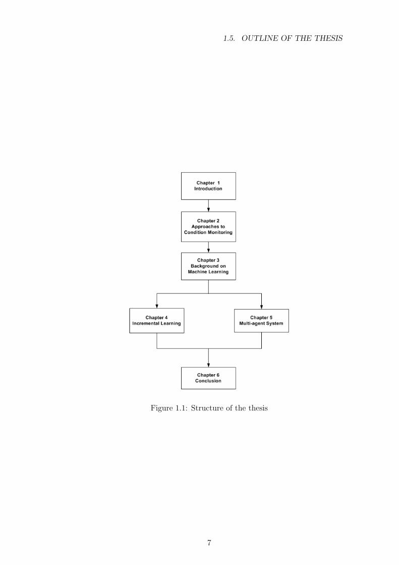
Figure 1.1 shows the layout of the dissertation. The reader is advised to
read the dissertation in a sequential way, however, due to the independence of
Chapter 4 and Chapter 5, these chapters can be read independently.
6
1.5. OUTLINE OF THE THESIS
Figure 1.1: Structure of the thesis
7

Chapter 2
Approaches to Condition
Monitoring
The aim of this chapter is to introduce the reader to aspects of condition
monitoring and various condition monitoring techniques. In this work, various
condition monitoring techniques are reviewed. The general framework of a
condition monitoring system that consists of the measurement stage, data
preprocessing and/or feature extraction stage and the classification stage is
outlined. A brief review of artificial intelligence (AI) techniques that have
been used for condition monitoring is also given.
2.1 Overview of Condition Monitoring
Condition monitoring of machines is gaining importance in industry due to
the need to increase machine reliability and decrease the possible loss of pro-
duction due to machine breakdown [11]. By definition, condition monitoring
is performed when it is necessary to access the state of a machine and to
determine whether it is malfunctioning through reason and observation [11].
Condition monitoring can also be defined as a technique or process of moni-
toring the operating characteristics of a machine so that changes and trends of
8

2.2. VARIOUS CONDITION MONITORING TECHNIQUES
the monitored signal can be used to predict the need for maintenance before a
breakdown or serious deterioration occurs, or to estimate the current condition
of the machine. Condition monitoring has become increasingly important, in
different industries due to an increased need for normal undisturbed opera-
tion of equipment. An unexpected fault or shutdown can result in a serious
accident and financial loss for the company. Hence, utilities must find ways
to avoid failures, minimize downtime, reduce maintenance costs, and lengthen
the lifetime of their equipment.
2.2 Various Condition Monitoring Techniques
There are numerous machine characteristics which can be monitored. Each of
these characteristics can be translated into a technique by which the condi-
tion of a machine is monitored. The condition monitoring techniques can be
roughly divided into the four categories electrical, chemical, vibrational and
temperature [3]. This research focuses only on analysis of information obtained
from chemical and vibration techniques.
2.2.1 Vibration-based Condition Monitoring
The most commonly used condition monitoring system is the vibration-based
condition monitoring [12]. The vibration monitoring technique is based on the
principle that all systems produce vibration. When a machine is operating
properly, vibration is small and constant; however, when faults develop and
some of the dynamic processes in the machine change, the vibration spectrum
also changes [13]. It is claimed that vibration monitoring is the most reliable
method of assessing the overall health of a rotating system [14]. Machines
have complex mechanical structures that oscillate and coupled parts of ma-
chines transmit these oscillations. This results in a machine related frequency
spectrum that characterizes healthy machine behavior. When a mechanical
9
2.2. VARIOUS CONDITION MONITORING TECHNIQUES
part of the machine either wears or breaks down, a frequency component in
the spectrum will change. Each fault in a rotating machine produces vibra-
tions with distinctive characteristics that can be measured and compared with
reference datasets in order to perform the fault detection and diagnosis pro-
cesses. Vibration monitoring system requires storing of a large amount of
data. Vibration is often measured with multiple sensors mounted on different
parts of the machine. For each machine there are typically several vibration
signals being analyzed in addition to static parameters such as load. The ex-
amination of data can be tedious and sensitive to errors. Also, fault related
machine vibration is usually corrupted with structural machine vibration and
noise from interfering machinery. Further, depending on the sensor position,
large deviations on noise may occur in measurements.
Various artificial intelligence techniques have been applied for vibration-based
condition monitoring. During the last years artificial neural network based
models like Multi-layer Perceptron (MLP) and Radial Basis Function (RBF)
have been used extensively for bearing condition monitoring. Samanta et al.
[14] used artificial neural network with time-domain features for rolling element
bearing detection. Yang et al. [15] applied the ART-KOHONEN to the prob-
lem of fault diagnosis of rotating machinery. Lately, kernel-based classifiers
such as Support Vector Machine have been used for bearing fault diagnosis.
Rojas and Nandi [16] used SVM for the detection and classification of rolling
element bearing faults. Samanta [17] used both ANN and SVM with genetic
algorithm for bearing fault detection. Yang et al. [18] used multi-class SVM
for fault diagnosis of rotating machinery. However, data-based statistical ap-
proaches such Gaussian mixture model and hidden Markov model (HMM) have
achieved considerable success in speech recognition and have been recently used
for condition monitoring. Ertunc et al. [19] used HMM to determine wear sta-
tus of the drill bits in a drilling process. Ocak and Loparo [20], Purushotham
et al. [21], Miao et al. [22] and Marwala et al. [23] used HMM for bearing fault
detection and diagnosis. In this work, vibration data set from motor bearing
is used.
10
2.2. VARIOUS CONDITION MONITORING TECHNIQUES
2.2.2 Dissolved Gas Analysis
Dissolved Gas analysis is one of the most popular chemical techniques that
are used in oil-filled equipment. DGA is the most commonly used diagnos-
tic technique for oil-filled machines such as transformers and bushings [24].
DGA is used to detect oil breakdown, moisture presence and partial discharge
activity. The gaseous byproduct are produced by degradation of transformer
and bushing oil and solid insulation, such as paper and pressboard, which are
all made of cellulose. The gases produced from the transformer and bushing
operation can be listed as follows [25]:
• Hydrocarbons and hydrogen gases: methane, ethane, ethylene, acetylene
and hydrogen.
• Carbon oxide: carbon monoxide and carbon dioxide.
• Naturally occurring gases: nitrogen and oxygen.
The symptoms of faults are classified into four main groups; corona, low energy
discharge, high energy discharge and thermal. The quantity and types of gases
reflect the nature and extent of the stressed mechanism in the bushing. Oil
breakdown is shown by the presence of hydrogen, methane, ethane, ethylene
and acetylene while high levels of hydrogen show that the degeneration is due
to corona. High levels of acetylene occur in the presence of arcing at high tem-
peratures. Methane and ethane are produced from low temperature thermal
heating of oil and high temperature thermal heating produces ethylene, hydro-
gen as well as a methane and ethane. Low temperature thermal degradation
of cellulose produces carbon dioxide and high temperature produces carbon
monoxide [24].
Existing diagnostic approaches for power transformers, which are based on the
dissolved gas information, can be divided into two categories; the conventional
approaches and artificial intelligence techniques.
11
2.2. VARIOUS CONDITION MONITORING TECHNIQUES
Conventional Approaches
Several renowned DGA interpretation schemes are; Drnenburg Ratios [26],
Rogers Ratios [27], Duval Triangle [28], and the IEC Ratios [29]. These
schemes have been implemented, either in modified format, by various power
utilities throughout the world. These schemes require computation of sev-
eral key gas ratios. Fault diagnosis is accomplished by associating the value
of these ratios with several predefined conditions of bushing. Two types of
incipient faults can be detected from these schemes; electrical fault and ther-
mal fault. Electrical fault can be divided into partial discharges and electrical
discharges [27], and examples of thermal fault are hot-spots and overheating.
A decision has to be made on whether fault diagnosis is necessary based on
the comparison of dissolved gas concentrations with a set of typical values of
gas concentration. If all dissolved gas concentrations are below these typical
values, then the power transformer concerned can be regarded as operating in
a normal manner.
2.2.3 Artificial Intelligence Approaches
Various attempts have been made to utilize AI techniques for diagnosis of
transformer condition based on the dissolved gas information [30, 31, 32, 33, 34,
35]. The intention of these approaches is to resolve some inherent limitations
of the conventional interpretation schemes and to improve the accuracy of
diagnosis.
Single AI Approaches
Single AI approaches only involve the utilization of one AI technique. The
most popular AI technique is the supervised artificial neural network (ANN).
A simple feed-forward ANN for detecting thermal and arcing faults is reported
12
2.2. VARIOUS CONDITION MONITORING TECHNIQUES
in [30]. Training samples were taken from post-mortem data and were carefully
selected so that various operating conditions were represented. It was reported
in [31] that more accurate diagnoses can be obtained, if compared to Rogers
Ratios and Drnenburg Ratios. Furthermore, two separate ANN were also used
in [32] for fault diagnosis and detection of cellulose degradation. It was found
that carbon dioxide and carbon monoxide are not needed as inputs for fault
diagnosis, and a single output that indicates whether cellulose was involved in
a fault is sufficient for the detection of cellulose degradation [31]. The same
authors also reported in the later publication [32] that higher diagnosis accu-
racy could be achieved if gas generation rates were included as inputs to the
ANN. While the aforementioned ANN-based approaches utilize actual DGA
data as training inputs, there are also other ANN-based approaches which
rely on conventional DGA interpretation schemes for generating the training
outputs. An example of such approaches can be found in [36], where key gas
concentrations, IEC Ratios, and Rogers Ratios were used to generate training
outputs for three independently trained ANN; fault diagnoses as given by these
ANN were combined to arrive at a final decision. The ANN-based approach, as
suggested in [33], relies totally on conventional interpretation scheme, where 13
characteristic patterns of gaseous composition were used as inputs to the ANN,
which was trained to detect different types of fault as specified in the Japanese
ECRA method. Unsupervised ANN were also implemented for the analysis
of the dissolved gas data. Specifically, self-organizing map was applied for ex-
ploratory analysis on historical DGA data [35]. It was reported that interesting
and comprehensive patterns have been unearthed, which could be associated
with certain incipient faults in power transformers. Kernel based approaches
such as Support Vector Machine (SVM) were also utilized for bushing fault
diagnosis [25]. The SVM approaches suggested in [25] rely on the conventional
DGA interpretation schemes for generating the training outputs.
13
2.2. VARIOUS CONDITION MONITORING TECHNIQUES
Hybrid AI Approaches
Other AI approaches applied for DGA interpretation are of hybrid nature
[36, 37, 38]. The use of a fuzzy expert system was reported in [37]; it was
implemented using if-then rules and fuzzy logic was introduced to resolve the
inherent uncertainties in normality thresholds, key-gas ratios, and concentra-
tions. The knowledge-base of the fuzzy expert system incorporates not only
popular DGA interpretation schemes such as Drnenburg Ratios, key gas con-
centrations, and IEC Ratios, but also synthetic expertise and heuristic main-
tenance rules based on expert experiences. Nevertheless, only a fairly simple
form of fuzzy concept was considered in [37] and a more general framework
associated with fuzzy measures and bodies of evidence was not pursued [38].
Consequently, a more general approach, known as the fuzzy information the-
ory, was proposed in [37] in order to systematically manage the uncertainties
that arise from different DGA interpretation schemes. In the fuzzy expert
system as reported in [37], each DGA interpretation scheme was represented
by several fuzzy rules; conflicts that arise between rules were resolved using
fuzzy information theory to find the most consistent solution. Diagnosis as
given by various schemes were combined to arrive at a final decision, in which
higher weights were attached to more certain diagnosis [32]. Although the
introduction of fuzzy concepts greatly improves the diagnosis accuracy of an
expert system, membership functions of fuzzy subsets are either determined
empirically or basically in a trial-and-error manner, where the conventional
DGA interpretation schemes are to be implicitly followed. Hence, a novel
approach known as the fuzzy evolutionary programming has been proposed
in [36], whereby conventional DGA interpretation schemes were used to con-
struct the preliminary framework of the fuzzy system, and an evolutionary
programming-based optimization algorithm was employed to further modify
the fuzzy if-then rules and simultaneously adjusting the membership functions
of the fuzzy subsets. Consequently, the cumbersome process of manually ad-
justing the fuzzy rules and membership functions can be avoided altogether.
14
2.2. VARIOUS CONDITION MONITORING TECHNIQUES
Limitation of Existing Approaches
There are several limitations pertaining to the foregoing ratio-based approaches.
Firstly, uncertainty and ambiguity still exist as to which key-gas ratios should
be considered and on the credibility of the suggested ratio values, since each
scheme has its own recommendation of key-gas ratios and their values [24].
Therefore, power utilities may have to adapt these ratio-based schemes heuris-
tically or on the experimental basis until satisfactory diagnoses are obtained.
Second, the heuristic and empirical nature of these ratio-based schemes have
brought about discrepancies in interpretation; application of different interpre-
tation schemes on identical set of DGA data may produce diverse diagnoses
of the transformer condition, thereby causing confusion among power utili-
ties. Lastly, the diagnosis of transformer condition is sometimes impossible to
achieve owing to the inability of these schemes to provide interpretation for ev-
ery possible combination of ratio values, with the exception of Duval Triangle
[28]. Consequently, the interpretation of a DGA data may have to depend on
expert judgement, which may instigate even more confusion since each expert
may have their own idea on what is happening inside the transformer based
on the dissolved gas information presented. It is known that supervised ANN
depend on either post-mortem data or conventional DGA schemes for training
outputs. However, the acquisition of a sufficient amount of post-mortem data
is difficult since it is too costly to dismantle a particular power transformer
for the purpose of investigating a suspected fault, since the transformer may
operate normally despite the increase in certain key gases. Consequently, there
might not be a lot of good cases for the training. Hybrid-AI approaches such as
fuzzy expert systems are used to tackle the ambiguity of conventional DGA in-
terpretation schemes, which are integrated into the foregoing approaches, and
expert experiences are incorporated to improve the credibility of diagnosis.
However, due to the incorporation of conventional schemes and expert expe-
riences, too many uncertainties are introduced to these approaches and would
thereby lead to the lack of confidence on final diagnoses if these uncertainties
15
2.3. COMPONENTS OF CONDITION MONITORING
were not managed appropriately. Furthermore, the aforementioned methods
do not have the capability to incrementally adapt over time, as new informa-
tion becomes available, or the systems being monitored undergo modifications.
This is essential since the monitoring system should be able to quickly adapt
to changes so as to maintain and improve system performance. Addition-
ally, these methods are too stable, they are incapable of incorporating new
experiences with minimal training time, and without overwriting (unlearning)
previous training experiences.
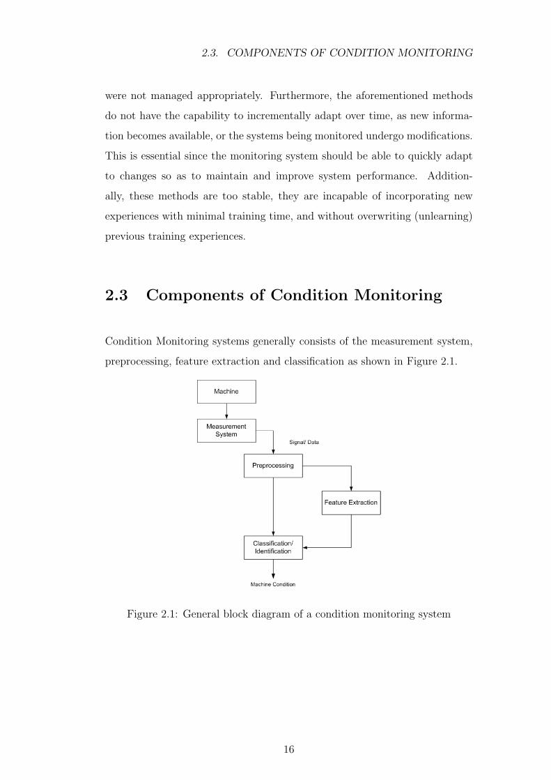
2.3 Components of Condition Monitoring
Condition Monitoring systems generally consists of the measurement system,
preprocessing, feature extraction and classification as shown in Figure 2.1.
Figure 2.1: General block diagram of a condition monitoring system
16
2.3. COMPONENTS OF CONDITION MONITORING
2.3.1 Measurement System and Preprocessing
Condition monitoring systems depend on sensors for obtaining the necessary
information. However, the odds of sensor failure are often of the same order of
magnitude as the odds of machinery failure. Since the diagnosis determined by
a condition monitoring system can only be accurate if the measured informa-
tion is correct, the first step should be to evaluate the sensor signals to ensure
that the correct signal is received. Direct methods are based on an evaluation
of the actual sensor signals. There are two methods that can be used for sensor
evaluation and these are; sensor redundancy and model-based methods [11].
Sensor redundancy aims to double redundant sensors can indicate the failure of
one of the sensors, but cannot tell which [11]. Triple redundant sensors in most
cases can locate the failing sensor [11]. Model-based methods use information
about the monitored machinery to create an analytic sensor redundancy. In-
stead of using two or more redundant sensors, the model will function as one
of the redundant sensors. These methods can identify less prominent sensor
faults than the direct methods mentioned above. Two successful model-based
methods that are used are; observer-based sensor monitoring and sensor fault
analysis. Observer-based sensor monitoring is based on models of parts of the
machinery and other sensor values, several observers calculate an estimate for
the value of a specific sensor. These estimated values are redundant with the
measured values and, thus, give an indication of a sensor fault. Sensor fault
analysis ensures that if a sensor fails, a characteristic pattern will appear in
the measured sensor data. This pattern is unique for a specific sensor fault.
2.3.2 Feature Extraction
Feature extraction is the process of representing a signal as a set of features
that lends itself to easy discrimination between pattern classes of the original
signal [39]. Feature extraction is a key component of any classification system
as it influences the complexity of the classification problem. If features do
17
2.3. COMPONENTS OF CONDITION MONITORING
not capture all relevant information that is necessary to distinguish between
pattern classes, reliable classification may be extremely difficult to achieve.
Features that contain too much information can sometimes be undesirable as
the additional, unnecessary information may confuse the classifier the classifi-
cation problem. In most classification systems, feature extraction also fulfills a
data reduction function by extracting features that are of a lower dimensional-
ity than the original signal. Generally, features in a lower dimensional feature
space are also easier to classify than features in a high dimensional feature
space and result in more computationally efficient classifiers. Another useful
property for feature extractors is to extract features that are invariant to sig-
nal amplitude and time. This may be advantageous for a time-varying signal.
Determining an optimal feature extraction method can be a challenging task
which is problem and classifier dependent.
Feature extraction techniques can be classified into three domains namely;
frequency domain analysis, time-frequency domain analysis and time domain
analysis [40]. The frequency domain methods often involve frequency analysis
of the signals and look at the periodicity of high frequency transients. The
frequency domain methods search for a train of ringings occurring at any of the
characteristic defect frequencies [12]. This procedure gets complicated consid-
ering the fact that the periodicity of the signal may be suppressed. These fre-
quency domain techniques include the frequency averaging technique, adaptive
noise cancellation and the high frequency resonance technique amongst others.
The main disadvantage of the frequency domain analysis is that it tends to
average out transient vibrations and therefore becomes more sensitive to back-
ground noise. To overcome this problem, the time-frequency domain analysis
is used which shows how the frequency contents of the signal changes with
time. The examples of such analysis are: Short Time Fourier Transform, the
Wigner-Ville Distribution and most commonly the Wavelet Transform. These
techniques are studied in detail in [12]. The last category of the feature extrac-
tion is the time domain analysis. Time domain methods usually involve indices
that are sensitive to impulsive oscillations, such as peak level, root mean square
18
2.3. COMPONENTS OF CONDITION MONITORING
value, crest factor analysis, kurtosis analysis, shock pulse counting, time series
averaging method, signal enveloping method and many more. In this study,
Mel-frequency Cepstral Coefficients (MFCC) and statistical features are used.
Mel-frequency Cepstral Coefficients
MFCCs have been widely used in the field of speech recognition and have
managed to represent the dynamic features of a signal as they extract both
linear and non-linear properties [41]. MFCC can be a useful tool of feature
extraction in vibration signals as vibrations contain both linear and non-linear
features. MFCC is a type of wavelet in which frequency scales are placed on a
linear scale for frequencies less than 1 kHz and on a log scale for frequencies
above 1 kHz [41]. The complex cepstral coefficients obtained from this scale
are called the MFCC [41]. The MFCC contain both time and frequency infor-
mation of the signal and this makes them more useful for feature extraction.
The following steps are involved in MFCC computations;
1. Transform input signal, x(n) from time domain to frequency domain by
applying Fast Fourier Transform (FFT), using [41]:
Y (m) =1
F
F−1∑n=0
x(n)w(n)e−j 2πf
nm (2.1)
Where F is the number of frames, and w(n) is the hamming window
function given by:
w(n) = β
(0.5− 0.5 cos
2πn
F − 1
)(2.2)
Where 0 ≤ n ≤ F − 1 and β is the normalization factor defined such
that the root mean square of the window is unity [41].
2. Mel-frequency wrapping is performed by changing the frequency to the
Mel using the following equation.
mel = 2595× log10
(1 +
fHz
700
)(2.3)
19
2.3. COMPONENTS OF CONDITION MONITORING
Mel-frequency warping uses a filter bank, spaced uniformly on the Mel
scale. The filter bank has a triangular band pass frequency response,
whose spacing and magnitude are determined by a constant Mel-frequency
interval.
3. The final step converts the logarithmic Mel spectrum back to the time
domain. The result of this step is what is called the Mel-frequency Cep-
stral Coefficients. This conversion is achieved by taking the Discrete
Cosine Transform of the spectrum as:
Cm =F−1∑n=0
cos(m
π
F(n + 0.5) log10(Hn)
)(2.4)
Where 0 ≤ m ≤ and L is the number of MFCC extracted form the ith
frame of the signal. Hn is the transfer function of the nth filter on the
filter bank.
These MFCC are then used as a representation of the signal.
Statistical Features
Basic statical features such as mean, root mean square, variance (σ), skew-
ness (normalized 3rd central moment) and kurtosis (normalized 4th central
moment) are implemented to obtain the signature of faults. The root mean
square value contains all the energy in the signal and therefore also all the noise
and all the elements that depend on the cutting process. Therefore, it is not
the most effective parameter but has retained its place because it is so easy to
produce and understand [14]. There is a need to deal with the occasional spik-
ing of vibration data, which is caused by some types of faults and to achieve
this task Kurtosis is used. The success of Kurtosis in signals is based on the
fact that signals of a system under stress or having defects differ from those
of a normal system. The sharpness or spiking of the vibration signal changes
when there are defects in the system. Kurtosis is a measure of the sharpness
20
2.3. COMPONENTS OF CONDITION MONITORING
of the peak and is defined as the normalized fourth-order central moment of
the signal [42]. The Kurtosis value is useful in identifying transients and spon-
taneous events within vibration signals and is one of the accepted criteria in
fault detection.
2.3.3 Classification
Condition classification includes the identification of the operating status of the
machine and type of failure by interpreting the representative system condition.
The classification system can be classified into two main groups, knowledge-
based and data-based models. Knowledge-based models rely on human-like
knowledge of the process and its faults. Knowledge-based models like expert
systems or decision trees apply human-like knowledge of the process for fault
diagnosis. In fault diagnostics, the human expert could be a person who oper-
ates the diagnosed machine or process and who is very well aware of different
kinds of faults occurring in it. Building the knowledge base can be achieved by
interviewing the human operator on faults occurring in the diagnosed machine
and on their symptoms. Expert systems are usually suitable for problems,
where a human expert can linguistically describe the solution. Typical hu-
man knowledge is vague and inexact, and handling this kind of information
has often been a problem with traditional expert systems. For example, the
limit when the temperature in a sauna is too high is vague in human mind.
In practice, it is very difficult to obtain adequate representations of the com-
plex and highly non-linear behavior of faulty plants using quantitative models.
Knowledge-based models may be utilized together with a simple signal-based
diagnostics, if the expert knowledge of the process is available. However, it
is often impossible even for a human expert to distinguish faults from the
healthy operation, and also multiple information sources may need to be used
for trustworthy decision making. Thus, the data-based models are the most
flexible approach to automated condition monitoring. Data-based models are
applied when the process model is not known in the analytical form and expert
21
2.4. CONDITION MONITORING ISSUES
knowledge of the process performance under faults is not available.
Learning machines must be adaptive if they have to operate effectively in
complex, real world problems. In many real-world applications, the knowl-
edge environment is non-stationary and the main assumption of a dynamic
work environment is that all information is not available a priori in the train-
ing set. The environment changes over time and requires that the learning
process tracks this change and includes it in its knowledge base. Building
a successful machine learning for a real-world problem might only be possi-
ble by incorporating the flexibility in acquiring the knowledge from each new
observation. It is possible to accomplish this task in reproducing entirely a
new knowledge base from the new observation plus all previous ones. This
solution is impractical since it requires the storage of all available training set
and a considerable computation time. Thus the system must learn from each
observation when it becomes available while preserving its current knowledge.
Incremental learning is a way to control the cost of knowledge update, it learns
from the new observation to adapt the previous knowledge to the changes in
the work environment. Incremental learning has a lot of advantages; it en-
ables learning of new observation, it adapts the knowledge base to the changes
of work environment and reinforces current knowledge. In Chapter 4, two
condition monitoring system that take advantages of incremental learning are
implemented.
2.4 Condition Monitoring Issues
Measurements from the system can be taken every few seconds. This leads
to an overwhelming volume of data per equipment to be interpreted by engi-
neers. When this is multiplied by the number of equipment to be monitored,
the problem of data overload becomes insurmountable in terms of manual data
interpretation. The second problem is the limited base of experts able to in-
terpret the complex condition monitoring data. The third issue is that most of
22
2.4. CONDITION MONITORING ISSUES
the time to effectively monitor the condition of a machine, more than one tech-
nology is used [7]. Thus, there is a longer term requirement for the integration
of further monitoring technologies.
Based on the problem, condition monitoring system identified above; the re-
quirements of an online condition monitoring system are [7]:
• The system must capture and condition the relevant data automatically.
• It should have the capacity to learn the typical plant behavior over a
period of time and then use this to indicate when anomalies and de-
fects arise and provide clear and concise defect information and remedial
advice to the operation engineer.
• It should have the ability to monitor changes and deviations in measure-
ments to allow differentiation between sensor defects and actual plant
defects.
• Extensibility and flexibility to include further interpretation techniques
and monitoring technologies.
The extensibility criterion is essential for longevity and practical implementa-
tion. The architecture must be scalable and support the introduction of new
sensors, data sets and interpretation techniques as they become available. This
requirement necessitates the use of intelligent and multi-agent system. For in-
stance, if requirements increase, agents can be added, replaced for better ones,
improved by providing agents with more experience or even having multiple
agents with the same goal working parallel, if one agent misses a symptom,
the other agent may observe it. Agents may also specialize of different tasks,
e.g. one agent may be an expert on partial discharge and another agent on
dissolved gas analysis, and then both agents may share some sensors or get
information from a sensor agent, an agent specialized in pre-processing the sen-
sor data and removing noise and other artifacts. Furthermore, new findings
23

2.4. CONDITION MONITORING ISSUES
and research results can be integrated into the relevant agents without any
redesign or modifications of the condition monitoring system. This suggests
that each of the required functions should be stand-alone, with the ability to
cooperate and exchange information as required. In Chapter 5, it is demon-
strated how the above requirements can be met using agents and multi-agent
system.
24
Chapter 3
Machine Learning
Machine learning has been used extensively in the area of condition monitoring
systems as described in the previous chapter. In this chapter, the theoretical
foundation of various machine learning tools such as Artificial Neural Networks
(ANN), Support Vector Machine (SVM), Extension Neural Network (ENN)
and Fuzzy ARTMAP (FAM) are briefly presented. As there are numerous
different types of ANNs, emphasis is given to the variant that is used in this
study called multi-Layer Perceptrons (MLPs). The design process for ensemble
of classifiers is outlined and the advantages of the ensemble approach are also
discussed.
3.1 Overview of Machine Learning
Machine learning is an area of artificial intelligence involving developing tech-
niques to allow computers to learn. More specifically, machine learning is a
method for creating computer programs by the analysis of data sets, rather
than the intuition of engineers. Machine learning algorithms are organized
into a taxonomy, based on the desired outcome of the algorithm. Common
algorithm types include [1]:
25
3.2. MACHINE LEARNING TOOLS
• Supervised - In the supervised paradigm a parameter update is based on
an error, given by the difference between the actual output y(t) = F (x(t))
and the target output y′(t). The target output is sometimes also called
teacher signal.
• Unsupervised - Learning without external signal or control.
• Reinforcement - In the reinforcement learning, a scalar reinforcement
signal is provided.
In all these three cases though, this learning can be represented mathemati-
cally, where for some input signal x(t) ∈ Rn and an output y(t) ∈ Rm for some
time step t ∈ N , the system learns a mapping F : Rn ⊃ X → Y ⊂ Rm or
simply x 7−→ y is learned [39]. The mapping F is usually a function defined
by some matrix of weight values.
3.2 Machine Learning Tools
3.2.1 Artificial Neural Network
ANNs are powerful data processing systems that are able to learn complex
input-output relationships from data. A typical ANN consists of a large num-
ber of simple processing elements called neurons that are highly interconnected
in an architecture that is loosely based on the structure of biological neurons
in the human or animal brain. A few attributes of interest are learning ability,
parallelism, distributed representation and computation, fault tolerance and
generalization ability. When used for pattern classification, the ANN performs
a nonlinear mapping function producing an output that indicates membership
of an input vector to a specific pattern class. The ANN learns this map-
ping function from training data and, if trained correctly, is able to generalize
on new data. This ability to learn from examples is useful for classification
26
3.2. MACHINE LEARNING TOOLS
problems that are too complex to be solved using algorithmic or rules-based
methods. There are several different types of ANN models that can be used
for classification. Two of the more commonly-used models are Multi-Layer
Perceptron (MLP) and Radial Basis Function (RBF) neural networks. MLP
networks generate a representation in the space of its hidden layer units that
is a more global and distributed representation of the input space than RBF
networks [1]. As a result, MLPs generally extrapolate better in regions of the
feature space that are not well represented by the training data. The disad-
vantage of using MLP networks is that they require more training time and
are more difficult to interpret than RBF networks [1]. In this work, MLP is
used.
Multi-layer Perceptron
ANNs provide a framework for representing nonlinear, parameterized mapping
functions between multi-dimensional spaces. The ANN learns a mapping func-
tion, F , from a set of training data such that F : x → y where x is a vector of
input variables and y is a vector of output variables. Learning is accomplished
by adjusting a set of ANN parameters called weights until a suitable response
is achieved. Each output, yk, of the ANN is, therefore, a function of its inputs,
x, and weights, w such that
yk = f(X; W ) (3.1)
In most cases, ANNs consist of simpler processing units called artificial neurons
arranged according to some topology [1]. Each input to the neuron is multiplied
by an adjustable weight parameter. The sum of all the weighted inputs is called
the activation of the neuron and is represented by
aj =N∑
i=0
wij × xij (3.2)
Where aj is the activation of neuron j, N is the number of inputs, xi, to
the neuron and wij is the weight parameter between input i and neuron j.
27
3.2. MACHINE LEARNING TOOLS
The input x0 is a special input, called a bias, that is always equal to 1. The
activation of the neuron becomes the input to a nonlinear activation function
which returns the output of the neuron
zj = f(aj) (3.3)
Where zj is the output of neuron j and f( · ) is the activation function. In
classification problems, common choices for the activation functions are the lo-
gistic sigmoid and hyperbolic tangent function. By itself, the single neuron has
limited data processing capabilities. In order to implement a useful mapping
function, multiple neurons are combined according to a network topology. For
computational reasons, the topology is restricted to a layered structure where
the outputs of all neurons in a lower layer become the inputs to each neuron
in the next higher layer.
For a MLP architecture with one neuron in the output layer, M neurons in the
hidden layer, and N inputs in the input layer, the response of the jth neuron
in the hidden layer can be derived from equations 3.2 and 3.3 as
y = fhidden(N∑
i=0
w1ijxi) (3.4)
where w1ij is the weight between input xi and hidden neuron j, w0j is the weight
of the bias input to neuron j and fhidden( · ) is the activation function. The
representational capability of the MLP refers to the range of mappings that
the MLP can implement as its weight parameters are varied. This indicates
whether the MLP is capable of implementing a desired mapping function. Pre-
vious work on this subject has shown that a sufficiently large network with a
sigmoidal activation function and one hidden layer of neurons is able to approx-
imate any function with arbitrary accuracy [1]. This universal approximation
capability proves that an MLP with one hidden layer is theoretically able to
implement any required mapping function. When used for classification, the
ANN is required to function as a statistical model of the process from which
the input data is generated. In order to realize this model, two problems have
28
3.2. MACHINE LEARNING TOOLS
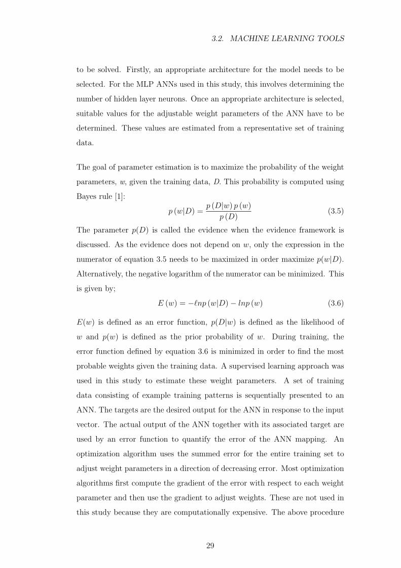
to be solved. Firstly, an appropriate architecture for the model needs to be
selected. For the MLP ANNs used in this study, this involves determining the
number of hidden layer neurons. Once an appropriate architecture is selected,
suitable values for the adjustable weight parameters of the ANN have to be
determined. These values are estimated from a representative set of training
data.
The goal of parameter estimation is to maximize the probability of the weight
parameters, w, given the training data, D. This probability is computed using
Bayes rule [1]:
p (w|D) =p (D|w) p (w)
p (D)(3.5)
The parameter p(D) is called the evidence when the evidence framework is
discussed. As the evidence does not depend on w, only the expression in the
numerator of equation 3.5 needs to be maximized in order maximize p(w|D).
Alternatively, the negative logarithm of the numerator can be minimized. This
is given by;
E (w) = −`np (w|D)− lnp (w) (3.6)
E(w) is defined as an error function, p(D|w) is defined as the likelihood of
w and p(w) is defined as the prior probability of w. During training, the
error function defined by equation 3.6 is minimized in order to find the most
probable weights given the training data. A supervised learning approach was
used in this study to estimate these weight parameters. A set of training
data consisting of example training patterns is sequentially presented to an
ANN. The targets are the desired output for the ANN in response to the input
vector. The actual output of the ANN together with its associated target are
used by an error function to quantify the error of the ANN mapping. An
optimization algorithm uses the summed error for the entire training set to
adjust weight parameters in a direction of decreasing error. Most optimization
algorithms first compute the gradient of the error with respect to each weight
parameter and then use the gradient to adjust weights. These are not used in
this study because they are computationally expensive. The above procedure
29
3.2. MACHINE LEARNING TOOLS
is repeated for many cycles called epochs until a satisfactory performance is
achieved. Once the error of the ANN on the training set of data and the
derivative of the error with respect to each weight parameter of the ANN have
been computed, an optimization algorithm can be used to adapt the weights
in order to minimize the error. For full details on artificial neural network, the
reader is referred to [1].
Figure 3.1: Architecture of the feed-forward multi-layer perceptron [1]
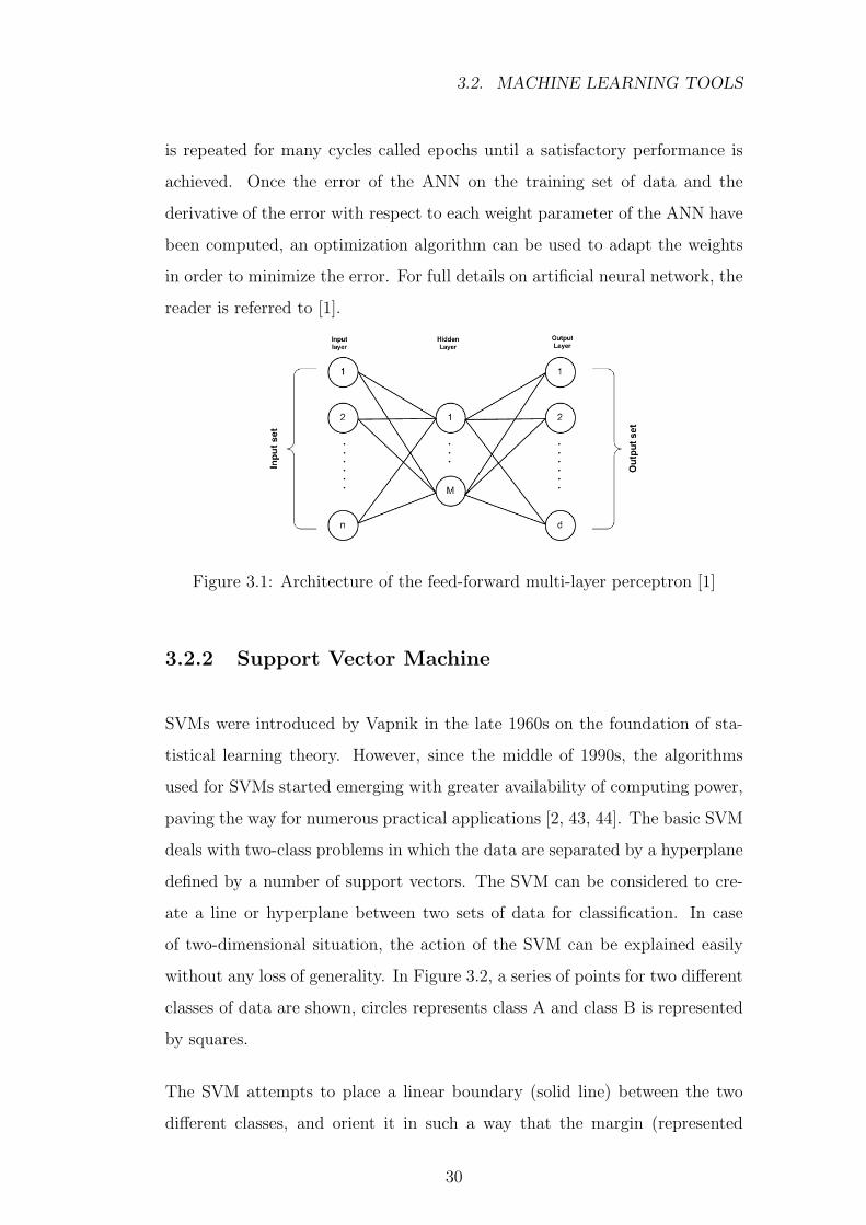
3.2.2 Support Vector Machine
SVMs were introduced by Vapnik in the late 1960s on the foundation of sta-
tistical learning theory. However, since the middle of 1990s, the algorithms
used for SVMs started emerging with greater availability of computing power,
paving the way for numerous practical applications [2, 43, 44]. The basic SVM
deals with two-class problems in which the data are separated by a hyperplane
defined by a number of support vectors. The SVM can be considered to cre-
ate a line or hyperplane between two sets of data for classification. In case
of two-dimensional situation, the action of the SVM can be explained easily
without any loss of generality. In Figure 3.2, a series of points for two different
classes of data are shown, circles represents class A and class B is represented
by squares.
The SVM attempts to place a linear boundary (solid line) between the two
different classes, and orient it in such a way that the margin (represented
30
3.2. MACHINE LEARNING TOOLS
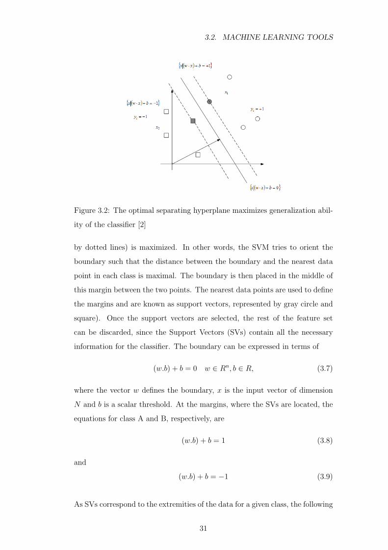
Figure 3.2: The optimal separating hyperplane maximizes generalization abil-
ity of the classifier [2]
by dotted lines) is maximized. In other words, the SVM tries to orient the
boundary such that the distance between the boundary and the nearest data
point in each class is maximal. The boundary is then placed in the middle of
this margin between the two points. The nearest data points are used to define
the margins and are known as support vectors, represented by gray circle and
square). Once the support vectors are selected, the rest of the feature set
can be discarded, since the Support Vectors (SVs) contain all the necessary
information for the classifier. The boundary can be expressed in terms of
(w.b) + b = 0 w ∈ Rn, b ∈ R, (3.7)
where the vector w defines the boundary, x is the input vector of dimension
N and b is a scalar threshold. At the margins, where the SVs are located, the
equations for class A and B, respectively, are
(w.b) + b = 1 (3.8)
and
(w.b) + b = −1 (3.9)
As SVs correspond to the extremities of the data for a given class, the following
31
3.2. MACHINE LEARNING TOOLS
decision function holds good for all data points belonging to either A or B:
f (x) = sign ((w.x) + b) (3.10)
The optimal hyperplane can be obtained as a solution to the optimization
problem, equation 3.11 is minimized
τ (w) =1
2‖w‖2 (3.11)
subject to
yi ((w.xi) + b) ≥ 1, i = 1 . . . l (3.12)
where l is the number of training sets. The solution of the constrained quadratic
programming optimization problem can be obtained as
w =∑
vixi (3.13)
where xi are SVs obtained from training. Putting equation 3.13 in equation
3.10 the decision function is obtained as follows:
f (x) = sign(∑
(vi (x ·xi)) + b)
(3.14)
In cases where the linear boundary in input spaces will not be enough to
separate two classes properly, it is possible to create a hyperplane that allows
linear separation in the higher dimension (corresponding to curved surface in
lower dimensional input space). In SVMs, this is achieved through the use of
a transformation that converts the data from an N-dimensional input space to
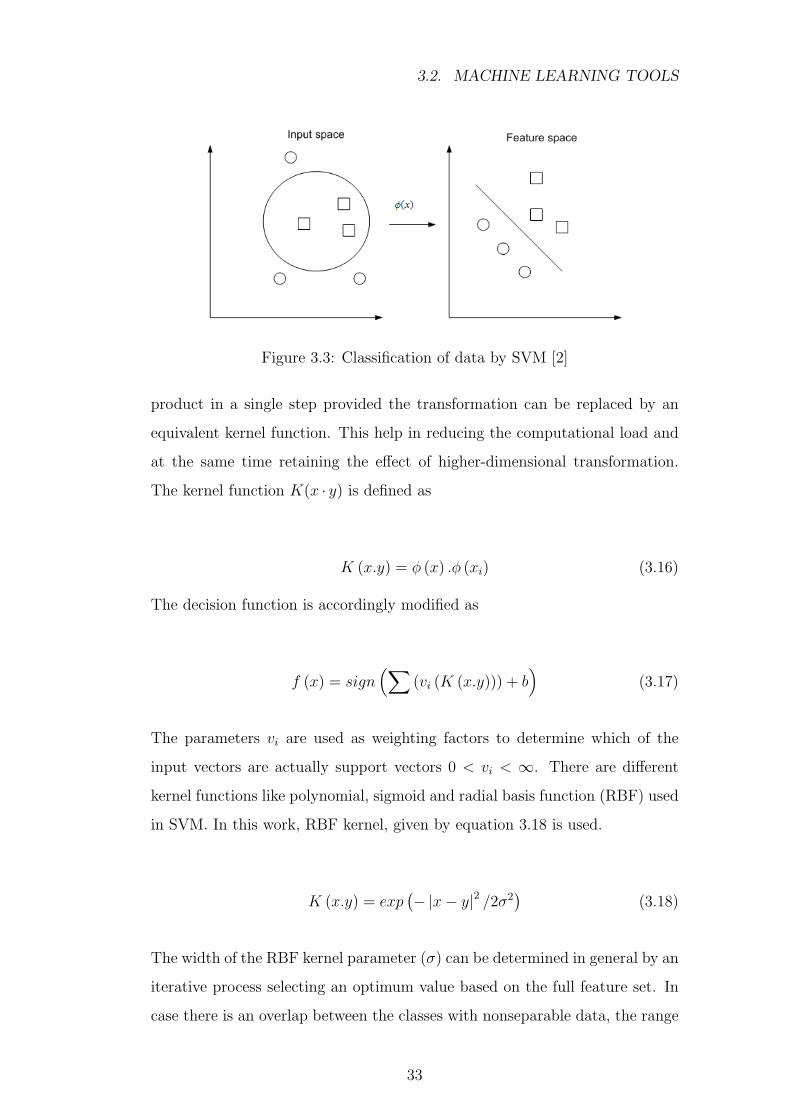
Q-dimensional feature space: s = φ (x) where x ∈ RN and s ∈ RQ: Figure 3.3
shows the transformation from input space to feature space where nonlinear
boundary has been transformed into a linear boundary in feature space.
Substituting the transformation in equation 3.14 gives
f (x) = sign(∑
(vi (φ (x) ·φ (xi))) + b)
(3.15)
The transformation into higher-dimensional feature space is relatively computation-
intensive. A kernel can be used to perform this transformation and the dot
32
3.2. MACHINE LEARNING TOOLS
Figure 3.3: Classification of data by SVM [2]
product in a single step provided the transformation can be replaced by an
equivalent kernel function. This help in reducing the computational load and
at the same time retaining the effect of higher-dimensional transformation.
The kernel function K(x · y) is defined as
K (x.y) = φ (x) .φ (xi) (3.16)
The decision function is accordingly modified as
f (x) = sign(∑
(vi (K (x.y))) + b)
(3.17)
The parameters vi are used as weighting factors to determine which of the
input vectors are actually support vectors 0 < vi < ∞. There are different
kernel functions like polynomial, sigmoid and radial basis function (RBF) used
in SVM. In this work, RBF kernel, given by equation 3.18 is used.
K (x.y) = exp(− |x− y|2 /2σ2
)(3.18)
The width of the RBF kernel parameter (σ) can be determined in general by an
iterative process selecting an optimum value based on the full feature set. In
case there is an overlap between the classes with nonseparable data, the range
33
3.2. MACHINE LEARNING TOOLS
of parameters vi can be limited to reduce the effect of outliers on the boundary
defined by SVs. For nonseparable case, the constraint is modified (0 < vi < C).
For separable case, C is infinity while for nonseparable case, it may be varied,
depending on the number of allowable errors in the trained solution: few errors
are permitted for high C while low C allows a higher proportion of errors in
the solution. To control generalization capability of SVM, there are a few free
parameters like limiting term C and the kernel parameters like RBF width.
For more details on SVM, the reader is referred to [2, 44, 45].
3.2.3 Extension Neural Network
The Extension Neural Network (ENN) is a new pattern classification system
based on concepts from neural networks and extension theory [46]. The ex-
tension theory uses a novel distance measurement for classification processes,
and the neural network can embed the salient features of parallel computation
power and learning capability. The classifier is well suited to classification
problems; where there exists patterns with a wide range of continuous inputs
and a discrete output indicating which class the pattern belongs to. The struc-
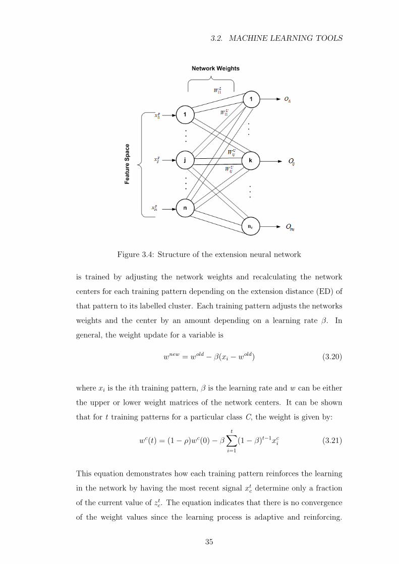
ture of the ENN is shown in Figure 3.4
ENN comprises of input layer and the output layer. The input layer nodes
receive an input feature pattern and uses a set of weighted parameters to
generate an image of the input pattern. There are two connection weights
between input nodes and output nodes; one connection represents the lower
bound for this classical domain of the features, and the other represents the
upper bound.The entire network is thus represented by a matrix of weights for
the upper and lower limits of the features for each class WU and WL. A third
matrix representing the cluster centers is also defined as [46]:
z =WU + WL
2(3.19)
ENN uses supervised learning, which tune the weights of the ENN to achieve a
good clustering performance or to minimize the clustering error. The network
34
3.2. MACHINE LEARNING TOOLS
Figure 3.4: Structure of the extension neural network
is trained by adjusting the network weights and recalculating the network
centers for each training pattern depending on the extension distance (ED) of
that pattern to its labelled cluster. Each training pattern adjusts the networks
weights and the center by an amount depending on a learning rate β. In
general, the weight update for a variable is
wnew = wold − β(xi − wold) (3.20)
where xi is the ith training pattern, β is the learning rate and w can be either
the upper or lower weight matrices of the network centers. It can be shown
that for t training patterns for a particular class C, the weight is given by:
wc(t) = (1− ρ)wc(0)− βt∑
i=1
(1− β)t−1xci (3.21)
This equation demonstrates how each training pattern reinforces the learning
in the network by having the most recent signal xtc determine only a fraction
of the current value of ztc. The equation indicates that there is no convergence
of the weight values since the learning process is adaptive and reinforcing.
35

3.2. MACHINE LEARNING TOOLS
Equation 3.21 also highlights the importance of the learning rate β. Small
values of β require many training epochs, whereas large values may results
in oscillatory behavior of the network weights, resulting in poor classification
performance.
3.2.4 Fuzzy ARTMAP
The fuzzy ARTMAP architecture is an auto-organized learning system [47].
This kind of network has supervised training and pertains to the adaptive res-
onance theory (ART) family; its structure is based on the adaptive resonance
theory and is similar to the fuzzy ART network, which employs calculus based
on fuzzy logic. This network is composed of two fuzzy ART modules; ARTa
and ARTb, interconnected by an inter-ART by an associative memory module
as illustrated in Figure 3.2.4 [47].
Figure 3.5: Structure of the fuzzy ARTMAP
A fuzzy ARTMAP has an internal controller that ensures autonomous system
36
3.2. MACHINE LEARNING TOOLS
operation in real time. The inter-ART module has a self-regulator mechanism
named match tracking, whose objective is to maximize the generalization and
minimize the network error. The F a2 layer is connected to the inter-ART
module by the weights wabjk. The input patterns of the ARTa is represented by
the vector a = [a1 . . . aMa] and the input patterns of the ARTb is represented
by the vector b = [b1 . . . bMb]. There are three fundamental parameters for the
performance and learning of the fuzzy ART network [47].
• The chosen parameter, (α > 0) which acts on the category selection.
• Training rate, (β ε [0, 1]) which controls the velocity or the learning rate
of the network adaptation, β = 1 permits the system to adapt faster
while 0 < β < 1 allows the system to adapt slower.
• Vigilance parameter, (ρ ε [0, 1]) which controls the network resonance.
The vigilance parameter is responsible for the number of categories formed.
If the vigilance parameter is very large, it produces a good classification,
providing the generation of several categories and this means that the
network has less errors but has less capacity for generalization. If it is
very small, it will generate few categories, which implies that the net-
work will have more capacity for generalization, but more possibility of
making mistakes.
The ART network affects the processing of two ART networks, ARTa and
ARTb, and after the resonance is confirmed in each network, J is the active
category for the ARTa network and K is the active category for the ARTb
network. The next step is to verify using the match tracking, if the active
category on ARTa corresponds to the desired output vector presented on ARTb.
The vigilance criterion is given by [47]:
|yb ∧ wabJK |
|yb|= ρab, (3.22)
It works by causing a little increment on the vigilance parameter only enough
to exclude that category and select another category which will be active and
37
3.3. ENSEMBLE OF CLASSIFIERS
reintroduced in the process until the active category correspond to the desired
output. After the input has completed the resonance state by the vigilance
criterion, the weight adaptation is effected. The adaptation of the ARTa and
ARTb module weights is given by [47]:
wnewJ = β(I ∧ wold
J ) + (1− β)woldJ , (3.23)
The adaptation for the inter-ART module is effected as follows [47]:
wabJK = 1,
wabJK = 0 for k 6= K
Full explanation of the Fuzzy ARTMAP algorithm can be found in Appendix
A.
3.3 Ensemble of Classifiers
Modeling using neural networks often involves trying multiple networks with
different architectures and training parameters in order to achieve acceptable
model accuracy. Selection of the best network is based on the performance
of the network on an independent validation or test set, and to keep only the
best performing network and to discard the rest. There are two disadvantages
with such an approach; first, all the effort involved in training the remaining
neural networks is wasted, second, the networks generalization performance is
greatly reduced. Ensemble approaches typically aim at improving the classifier
accuracy on a complex classification problem through a divide-and-conquer
approach. Perrone and Copper [48] proved mathematically that an ensemble
method can be used to improve the classification ability of a single classifier.
They argue that the ensemble method have the following advantages:
1. It efficiently uses all the networks in the population - none of the network
need to be discarded.
2. It uses all the available data for training without overfitting.
38
3.3. ENSEMBLE OF CLASSIFIERS
3. It performs regularization by smoothing in functional space which helps
with overfitting.
4. It is suited for parallel computing.
In essence, a group of simple classifiers is generated typically from boot-
strapped, jackknifed, or bagged replicas of the training data or by changing
other design parameters of the classifier, which are combined through a clas-
sifier combination scheme, such as the weighted majority voting [49]. The
ensemble generally is formed from weak classifiers to take advantage of their
so called instability [49]. This instability promotes diversity in the classifiers
by forcing them to construct sufficiently different decision boundaries (clas-
sification rules) for minor modifications in their training datasets, which in
turn causes each classifier to make different errors on any given instance. A
strategic combination of these classifiers then eliminates the individual errors,
generating a strong classifier. The success of an ensemble method depends on
two factors; a pool of diverse individual classifiers to be fused and a proper de-
cision fusion method. A proper classifier team should be robust and generate
the best fusion performance. It should also be optimal so that it can reduce
the time for calculation while improving the classification accuracy. Figure 3.6
shows the flowchart of decision-level fusion.
3.3.1 Classifier Selection Methods
Various classifier selection techniques such as Q static, generalized diversity
and agreement have been used successfully for classifier selection [50, 51]. Many
researchers have found that the dependency among classifiers can affect the
fusion results. Goebel et al. [52] recommended an effective method for classifier
selection based on calculating the correlation degree of n classifiers. This
method is used to select the classifiers to be fused. This correlation degree is
39
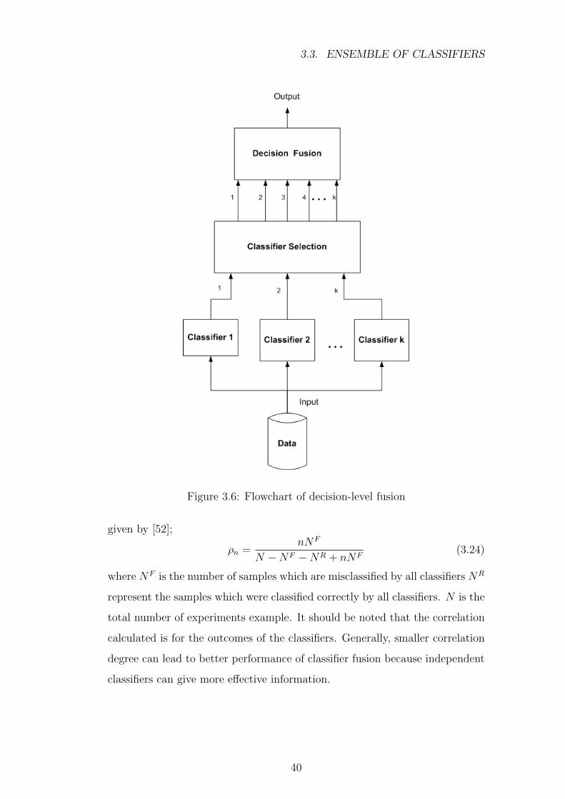
3.3. ENSEMBLE OF CLASSIFIERS
Figure 3.6: Flowchart of decision-level fusion
given by [52];
ρn =nNF
N −NF −NR + nNF(3.24)
where NF is the number of samples which are misclassified by all classifiers NR
represent the samples which were classified correctly by all classifiers. N is the
total number of experiments example. It should be noted that the correlation
calculated is for the outcomes of the classifiers. Generally, smaller correlation
degree can lead to better performance of classifier fusion because independent
classifiers can give more effective information.
40

3.3. ENSEMBLE OF CLASSIFIERS
3.3.2 Decision Fusion Methods
A number of researchers have investigated the properties of combined classi-
fiers. Wolpert introduced the idea of combining hierarchical levels of classifiers,
using a procedure called stacked generalization [53]. Kitler et al. [54] analyzed
error sensitivities of various voting and combination schemes, whereas Ran-
garajan et al. [55] investigated the capacity of voting systems. Ji and Ma [56]
also gave an excellent review of various methods for combining classifiers.
41
Chapter 4
Incremental Learning and its
Application to Condition
Monitoring
The problem of fault diagnosis of machine has been an ongoing research in vari-
ous industries. Many machine learning tools have been applied to this problem
using static machine learning structures such as neural network and support
vector machine that are unable to accommodate new information as it becomes
available into their existing models. The chapter introduces the incremental
learning approach to the problem of condition monitoring. The chapter starts
by giving a brief definition of incremental learning. Two incremental learn-
ing techniques are applied to the problem of condition monitoring. The first
method uses the incremental learning ability of Fuzzy ARTMAP (FAM) and
explores whether ensemble approach can improve the performance of the FAM.
The second technique uses Learn++ that uses an ensemble of MLP classifiers.
Lastly, these two methods are compared with each others.
42
4.1. INCREMENTAL LEARNING
4.1 Incremental Learning
An incremental learning algorithm is an algorithm that is able to learn addi-
tional information from data while retaining previously learned information.
The algorithm should not require access to the original data and must also be
able to learn classes that may be introduced by incoming data. The FAM and
Learn++ fulfill all these criteria.
The characterization of machine incremental learning applies to three dimen-
sions of machine incremental learning; structural changes, learning parameter
adjustments and input data variations. In characterization, let s = (si)i=0...n,
l = (lj)j=0...n and d = (dk)k=0...n be families of real numbers. An incremental
learning system I = (s; l; d) is a learning system which is parameterized by
three families of incremental learning parameters which can be modified dur-
ing training [57]. The first is the structure parameters (s = (si)i=0...n), which
are, for example, the number of neurons, density of connections, or other pa-
rameters which determine structure and functionality of a neural network.
Learning parameters (l = (lj)j=0...n) which are, for example, evolutionary or
other learning parameters, such as the stepsize. Data-complexity parameters
(d = (dk)k=0...n) which can represent any complexity measure of the training
data. Accordingly, there are three main forms of incremental learning. Each
of them modifies members of one of the parameter families defined above [57]:
• Structure Incremental Learning: The structure or functional capacity of
the neural network is changed during learning.
• Learning Parameter Incremental Learning: A selection of learning pa-
rameters from l = (lj) is adapted during learning.
• Data Incremental Learning: The data set or its complexity is increased
in stages during learning controlled by parameter changes of d = (dk).
The incremental learning in the fuzzy ARTMAP is a combination of structure
43
4.1. INCREMENTAL LEARNING
and data incremental learning. As data of different classes is added to the
system or more data on existing classes are added, the structure of the sys-
tem adapts creating a larger number of categories in which to map the output
labels. The incremental learning in Learn++ is a data incremental learning
because as new data is added new classifiers are build to be added to the
existing system. Learning new information without requiring access to previ-
ously used data, however, raises “stability-plasticity dilemma”. This dilemma
indicates that a completely stable classifier maintains the knowledge from pre-
viously seen data, but fails to adjust in order to learn new information, while
a completely plastic classifier is capable of learning new data but lose prior
knowledge.
Various incremental learning algorithms have been developed. Notable exam-
ples of incremental learning include growing neural network architectures one
node at a time [58, 59]. Another group of algorithms that claim incremental
learning are those that modify the weights of a neural network architecture
by retraining, typically with misclassified signals. Although, these schemes
are closer in meaning to the definition of incremental learning, however, they
violate the major requirement since they forget previous learning and require
access to old data. Vo [60] describes an incremental learning algorithm for
time delay neural networks , which supplements the original time delay neural
network architecture with the capability of learning a misclassified pattern in a
single epoch by adding a dedicated hidden layer unit. Hoya and Constantinides
[61] describe an incremental learning scheme for generalized recursive neural
network and related family of networks such as probabilistic neural network
and exact RBF networks; however, this algorithm does not learn new patterns
but rather previously misclassified patterns. Higgins and Goodman [62] have
suggested incremental learning with a rule based network, which actually has
the same fundamental idea of the work described in [61]. The algorithm in-
volves growing a network incrementally using the new data without requiring
old data. Chen and Soo [63] introduced an incremental feed-forward neural
network which involves learning of one additional instance given a previously
44
4.2. FUZZY ARTMAP AND INCREMENTAL LEARNING
trained network. They update the weights for the additional instance in such a
way that the influence of the weight update on previously trained instances is
minimum, which is satisfied by minimizing a weight-sensitivity cost function.
Fu et al. [64, 65] introduced an incremental backpropagation learning network
that is capable of learning new data in the absence of old data. However,
this system, also based on learning new instances through minor modification
of current weights by putting a bound on weight modification, is not able to
learn new classes. Various methods have been proposed for incremental SVM
learning in the literature [66, 67].
4.2 Fuzzy ARTMAP and Incremental Learn-
ing
4.2.1 System Design
The proposed system is implemented using the fuzzy ARTMAP. The overview
of the proposed system is shown in Figure 4.1. The population of classifiers is
used to introduce classification diversity. A bad team of classifiers may even
lead to worse performance than the best single classifier due to the fusion of
error decision. A classifier selection process is executed using the correlation
measure. After the classifier selection, majority voting fusion algorithm is
employed for the final decision.
Data Preprocessing
The variables undergo a min-max normalization. The normalization is a re-
quirement for using the FAM, since the FAM complement coding assumed
the data is normalized. The equation for min-max normalization for a single
45
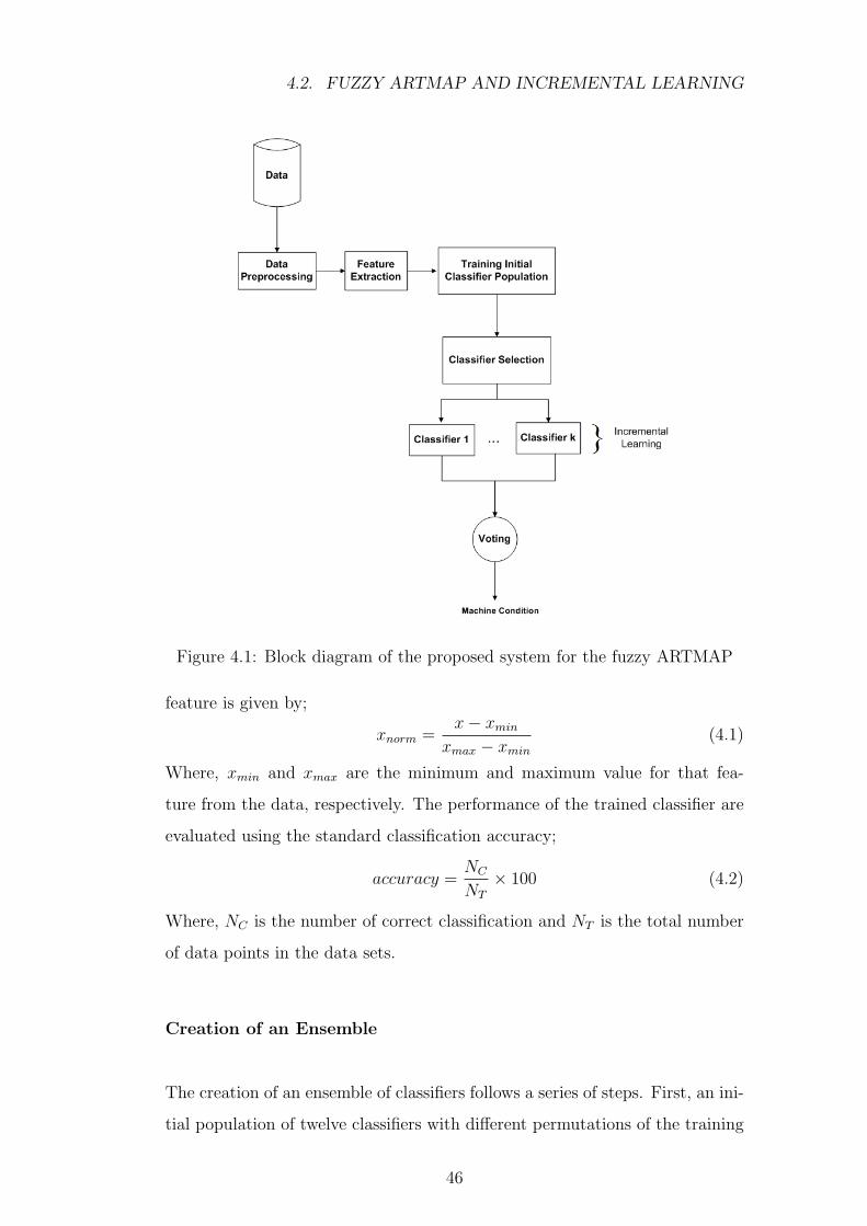
4.2. FUZZY ARTMAP AND INCREMENTAL LEARNING
Figure 4.1: Block diagram of the proposed system for the fuzzy ARTMAP
feature is given by;
xnorm =x− xmin
xmax − xmin
(4.1)
Where, xmin and xmax are the minimum and maximum value for that fea-
ture from the data, respectively. The performance of the trained classifier are
evaluated using the standard classification accuracy;
accuracy =NC
NT
× 100 (4.2)
Where, NC is the number of correct classification and NT is the total number
of data points in the data sets.
Creation of an Ensemble
The creation of an ensemble of classifiers follows a series of steps. First, an ini-
tial population of twelve classifiers with different permutations of the training
46
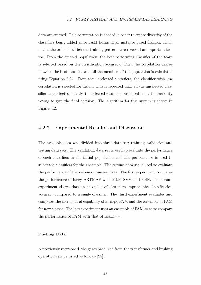
4.2. FUZZY ARTMAP AND INCREMENTAL LEARNING
data are created. This permutation is needed in order to create diversity of the
classifiers being added since FAM learns in an instance-based fashion, which
makes the order in which the training patterns are received an important fac-
tor. From the created population, the best performing classifier of the team
is selected based on the classification accuracy. Then the correlation degree
between the best classifier and all the members of the population is calculated
using Equation 3.24. From the unselected classifiers, the classifier with low
correlation is selected for fusion. This is repeated until all the unselected clas-
sifiers are selected. Lastly, the selected classifiers are fused using the majority
voting to give the final decision. The algorithm for this system is shown in
Figure 4.2.
4.2.2 Experimental Results and Discussion
The available data was divided into three data set; training, validation and
testing data sets. The validation data set is used to evaluate the performance
of each classifiers in the initial population and this performance is used to
select the classifiers for the ensemble. The testing data set is used to evaluate
the performance of the system on unseen data. The first experiment compares
the performance of fuzzy ARTMAP with MLP, SVM and ENN. The second
experiment shows that an ensemble of classifiers improve the classification
accuracy compared to a single classifier. The third experiment evaluates and
compares the incremental capability of a single FAM and the ensemble of FAM
for new classes. The last experiment uses an ensemble of FAM so as to compare
the performance of FAM with that of Learn++.
Bushing Data
A previously mentioned, the gases produced from the transformer and bushing
operation can be listed as follows [25]:
47

4.2. FUZZY ARTMAP AND INCREMENTAL LEARNING
TRAINING PHASE
1. Create a population of 12 classifiers with different permutation of the
input data.
2. Select an appropriate performance measure as the initial evaluation crite-
rion such as accuracy rate, which is the ratio. number of sample classified
correctly to the total sample.
3. Find the best performing classifiers to be the first classifier of the ensem-
ble.
4. Calculate the correlation degree between the first classifier and other
classifiers, respectively using Equation 3.24
5. Select the classifier with low correlation for fusion. 6 Repeat 4 and 5
between selected classifiers yet to be selected until all the classifiers are
determined.
6. Fuse the individual classifier’s prediction using majority voting strategy.
OPERATION PHASE
1. If a new data becomes available during the operation phase.
2. Add new data to the ensemble of classifiers by training the individual
classifier and then combine through majority voting.
Figure 4.2: The algorithm for the fuzzy ARTMAP system
• Hydrocarbons and hydrogen gases: methane , ethane, ethylene, acetylene
and hydrogen.
• Carbon oxide: carbon monoxide and carbon dioxide.
• Naturally occurring gases: nitrogen and oxygen
48
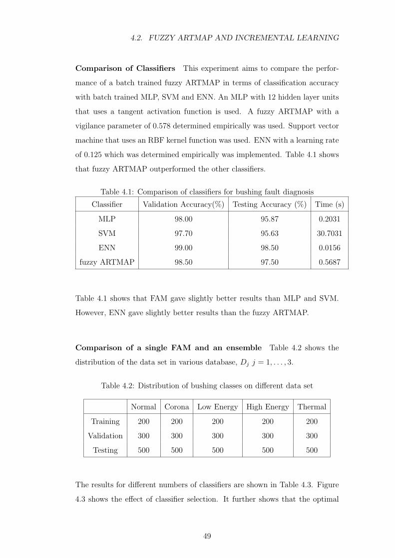
4.2. FUZZY ARTMAP AND INCREMENTAL LEARNING
Comparison of Classifiers This experiment aims to compare the perfor-
mance of a batch trained fuzzy ARTMAP in terms of classification accuracy
with batch trained MLP, SVM and ENN. An MLP with 12 hidden layer units
that uses a tangent activation function is used. A fuzzy ARTMAP with a
vigilance parameter of 0.578 determined empirically was used. Support vector
machine that uses an RBF kernel function was used. ENN with a learning rate
of 0.125 which was determined empirically was implemented. Table 4.1 shows
that fuzzy ARTMAP outperformed the other classifiers.
Table 4.1: Comparison of classifiers for bushing fault diagnosis
Classifier Validation Accuracy(%) Testing Accuracy (%) Time (s)
MLP 98.00 95.87 0.2031
SVM 97.70 95.63 30.7031
ENN 99.00 98.50 0.0156
fuzzy ARTMAP 98.50 97.50 0.5687
Table 4.1 shows that FAM gave slightly better results than MLP and SVM.
However, ENN gave slightly better results than the fuzzy ARTMAP.
Comparison of a single FAM and an ensemble Table 4.2 shows the
distribution of the data set in various database, Dj j = 1, . . . , 3.
Table 4.2: Distribution of bushing classes on different data set
Normal Corona Low Energy High Energy Thermal
Training 200 200 200 200 200
Validation 300 300 300 300 300
Testing 500 500 500 500 500
The results for different numbers of classifiers are shown in Table 4.3. Figure
4.3 shows the effect of classifier selection. It further shows that the optimal
49
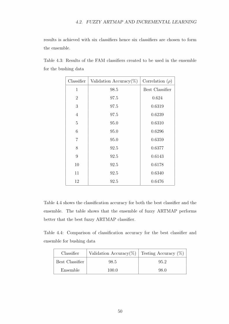
4.2. FUZZY ARTMAP AND INCREMENTAL LEARNING
results is achieved with six classifiers hence six classifiers are chosen to form
the ensemble.
Table 4.3: Results of the FAM classifiers created to be used in the ensemble
for the bushing data
Classifier Validation Accuracy(%) Correlation (ρ)
1 98.5 Best Classifier
2 97.5 0.624
3 97.5 0.6319
4 97.5 0.6239
5 95.0 0.6310
6 95.0 0.6296
7 95.0 0.6359
8 92.5 0.6377
9 92.5 0.6143
10 92.5 0.6178
11 92.5 0.6340
12 92.5 0.6476
Table 4.4 shows the classification accuracy for both the best classifier and the
ensemble. The table shows that the ensemble of fuzzy ARTMAP performs
better that the best fuzzy ARTMAP classifier.
Table 4.4: Comparison of classification accuracy for the best classifier and
ensemble for bushing data
Classifier Validation Accuracy(%) Testing Accuracy (%)
Best Classifier 98.5 95.2
Ensemble 100.0 98.0
50
4.2. FUZZY ARTMAP AND INCREMENTAL LEARNING
Figure 4.3: The effect of classifier selection
Incremental Learning Any condition monitoring system that has to be
used online must have incremental learning capability for it to be rendered
useful. As mentioned earlier an incremental learning algorithm must accom-
modate both new data and new classes that may be present in the new data
without compromising the classification accuracy of the previously learned
data. Carpenter et al. [47] showed that the fuzzy ARTMAP is able to accom-
modate these types of data.
The incremental learning capability of a single FAM is compared with that of
an ensemble of classifiers. For the initial experiment the knowledge of a fourth
class is added to the classification system. Using the existing model of the
classifier in the ensemble, each classifier is trained on data of this new class.
Experimentation is performed on independent test set for this class for both
the best classifier and ensemble of the classifiers. Both the best classifier and
the ensemble gave a classification accuracy of 100%. Experimentation of the
system on the testing data set of the initial three classes is performed, this
is to determine how addition of new information affects previously learned
information. The classifier accuracy achieved is 94.88% for the best classifier
51
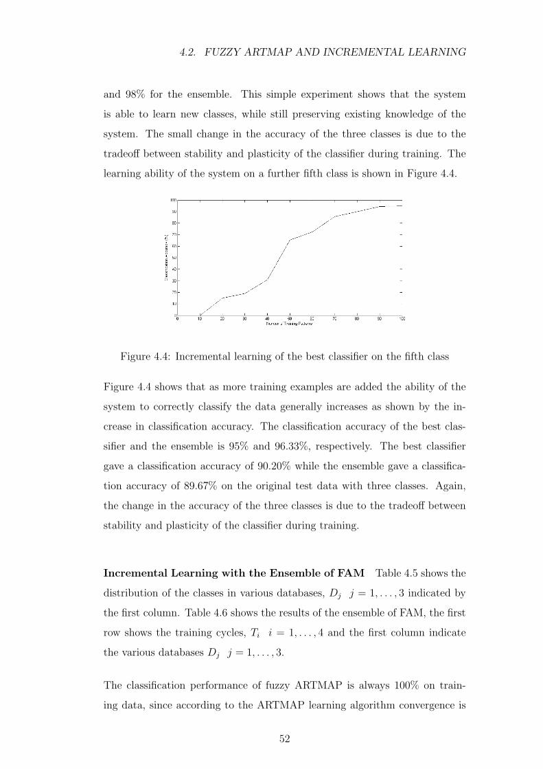
4.2. FUZZY ARTMAP AND INCREMENTAL LEARNING
and 98% for the ensemble. This simple experiment shows that the system
is able to learn new classes, while still preserving existing knowledge of the
system. The small change in the accuracy of the three classes is due to the
tradeoff between stability and plasticity of the classifier during training. The
learning ability of the system on a further fifth class is shown in Figure 4.4.
Figure 4.4: Incremental learning of the best classifier on the fifth class
Figure 4.4 shows that as more training examples are added the ability of the
system to correctly classify the data generally increases as shown by the in-
crease in classification accuracy. The classification accuracy of the best clas-
sifier and the ensemble is 95% and 96.33%, respectively. The best classifier
gave a classification accuracy of 90.20% while the ensemble gave a classifica-
tion accuracy of 89.67% on the original test data with three classes. Again,
the change in the accuracy of the three classes is due to the tradeoff between
stability and plasticity of the classifier during training.
Incremental Learning with the Ensemble of FAM Table 4.5 shows the
distribution of the classes in various databases, Dj j = 1, . . . , 3 indicated by
the first column. Table 4.6 shows the results of the ensemble of FAM, the first
row shows the training cycles, Ti i = 1, . . . , 4 and the first column indicate
the various databases Dj j = 1, . . . , 3.
The classification performance of fuzzy ARTMAP is always 100% on train-
ing data, since according to the ARTMAP learning algorithm convergence is
52
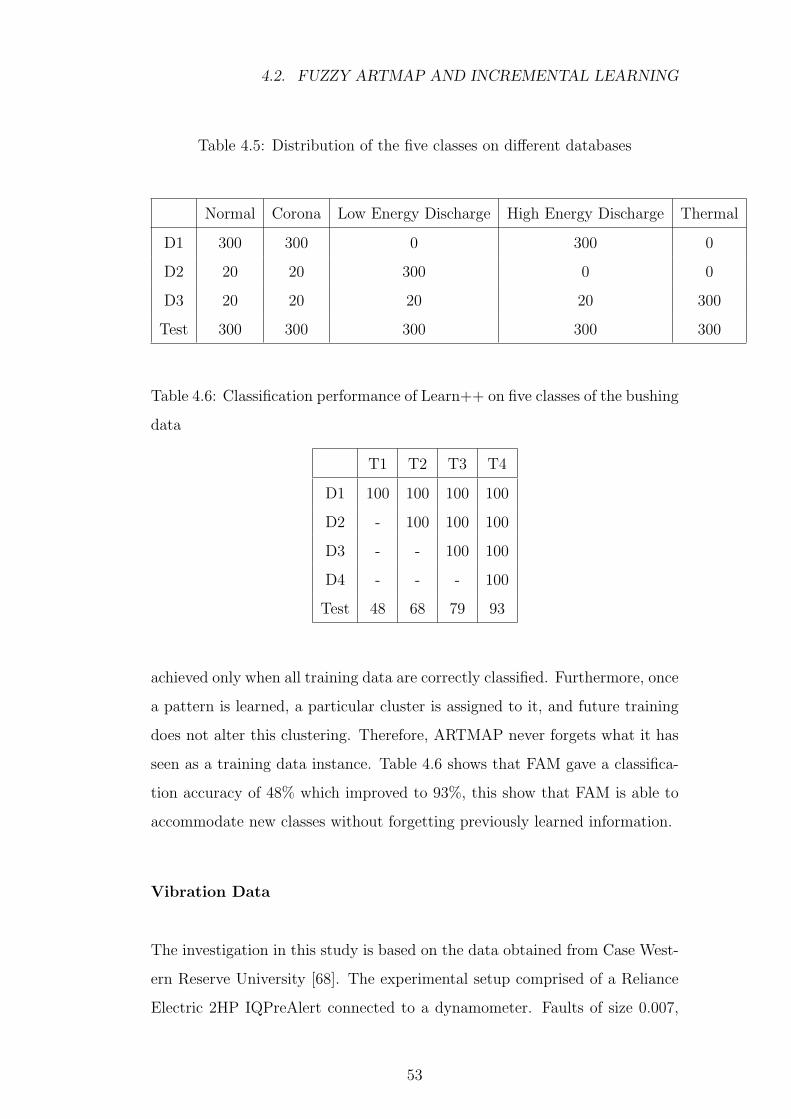
4.2. FUZZY ARTMAP AND INCREMENTAL LEARNING
Table 4.5: Distribution of the five classes on different databases
Normal Corona Low Energy Discharge High Energy Discharge Thermal
D1 300 300 0 300 0
D2 20 20 300 0 0
D3 20 20 20 20 300
Test 300 300 300 300 300
Table 4.6: Classification performance of Learn++ on five classes of the bushing
data
T1 T2 T3 T4
D1 100 100 100 100
D2 - 100 100 100
D3 - - 100 100
D4 - - - 100
Test 48 68 79 93
achieved only when all training data are correctly classified. Furthermore, once
a pattern is learned, a particular cluster is assigned to it, and future training
does not alter this clustering. Therefore, ARTMAP never forgets what it has
seen as a training data instance. Table 4.6 shows that FAM gave a classifica-
tion accuracy of 48% which improved to 93%, this show that FAM is able to
accommodate new classes without forgetting previously learned information.
Vibration Data
The investigation in this study is based on the data obtained from Case West-
ern Reserve University [68]. The experimental setup comprised of a Reliance
Electric 2HP IQPreAlert connected to a dynamometer. Faults of size 0.007,
53
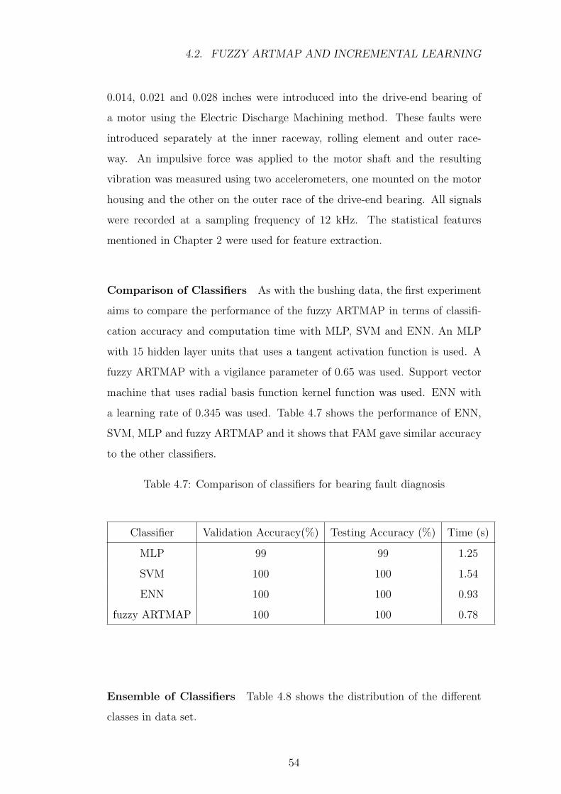
4.2. FUZZY ARTMAP AND INCREMENTAL LEARNING
0.014, 0.021 and 0.028 inches were introduced into the drive-end bearing of
a motor using the Electric Discharge Machining method. These faults were
introduced separately at the inner raceway, rolling element and outer race-
way. An impulsive force was applied to the motor shaft and the resulting
vibration was measured using two accelerometers, one mounted on the motor
housing and the other on the outer race of the drive-end bearing. All signals
were recorded at a sampling frequency of 12 kHz. The statistical features
mentioned in Chapter 2 were used for feature extraction.
Comparison of Classifiers As with the bushing data, the first experiment
aims to compare the performance of the fuzzy ARTMAP in terms of classifi-
cation accuracy and computation time with MLP, SVM and ENN. An MLP
with 15 hidden layer units that uses a tangent activation function is used. A
fuzzy ARTMAP with a vigilance parameter of 0.65 was used. Support vector
machine that uses radial basis function kernel function was used. ENN with
a learning rate of 0.345 was used. Table 4.7 shows the performance of ENN,
SVM, MLP and fuzzy ARTMAP and it shows that FAM gave similar accuracy
to the other classifiers.
Table 4.7: Comparison of classifiers for bearing fault diagnosis
Classifier Validation Accuracy(%) Testing Accuracy (%) Time (s)
MLP 99 99 1.25
SVM 100 100 1.54
ENN 100 100 0.93
fuzzy ARTMAP 100 100 0.78
Ensemble of Classifiers Table 4.8 shows the distribution of the different
classes in data set.
54
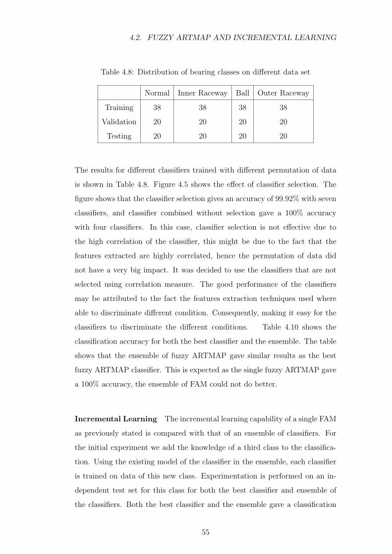
4.2. FUZZY ARTMAP AND INCREMENTAL LEARNING
Table 4.8: Distribution of bearing classes on different data set
Normal Inner Raceway Ball Outer Raceway
Training 38 38 38 38
Validation 20 20 20 20
Testing 20 20 20 20
The results for different classifiers trained with different permutation of data
is shown in Table 4.8. Figure 4.5 shows the effect of classifier selection. The
figure shows that the classifier selection gives an accuracy of 99.92% with seven
classifiers, and classifier combined without selection gave a 100% accuracy
with four classifiers. In this case, classifier selection is not effective due to
the high correlation of the classifier, this might be due to the fact that the
features extracted are highly correlated, hence the permutation of data did
not have a very big impact. It was decided to use the classifiers that are not
selected using correlation measure. The good performance of the classifiers
may be attributed to the fact the features extraction techniques used where
able to discriminate different condition. Consequently, making it easy for the
classifiers to discriminate the different conditions. Table 4.10 shows the
classification accuracy for both the best classifier and the ensemble. The table
shows that the ensemble of fuzzy ARTMAP gave similar results as the best
fuzzy ARTMAP classifier. This is expected as the single fuzzy ARTMAP gave
a 100% accuracy, the ensemble of FAM could not do better.
Incremental Learning The incremental learning capability of a single FAM
as previously stated is compared with that of an ensemble of classifiers. For
the initial experiment we add the knowledge of a third class to the classifica-
tion. Using the existing model of the classifier in the ensemble, each classifier
is trained on data of this new class. Experimentation is performed on an in-
dependent test set for this class for both the best classifier and ensemble of
the classifiers. Both the best classifier and the ensemble gave a classification
55
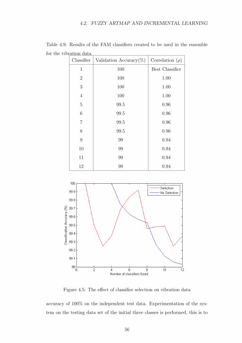
4.2. FUZZY ARTMAP AND INCREMENTAL LEARNING
Table 4.9: Results of the FAM classifiers created to be used in the ensemble
for the vibration data
Classifier Validation Accuracy(%) Correlation (ρ)
1 100 Best Classifier
2 100 1.00
3 100 1.00
4 100 1.00
5 99.5 0.96
6 99.5 0.96
7 99.5 0.96
8 99.5 0.96
9 99 0.94
10 99 0.94
11 99 0.94
12 99 0.94
Figure 4.5: The effect of classifier selection on vibration data
accuracy of 100% on the independent test data. Experimentation of the sys-
tem on the testing data set of the initial three classes is performed, this is to
56
4.2. FUZZY ARTMAP AND INCREMENTAL LEARNING
Table 4.10: Comparison of classification accuracy for the best classifier and
ewnsemble for the vibration data
Classifier Validation Accuracy(%) Testing Accuracy (%)
Best Classifier 100 100
Ensemble 100 100
determine how addition of new information affects previously learned informa-
tion. The classifier accuracy achieved is 98% for the best classifier and 100%
for the ensemble. This simple experiment shows that the system is able to
learn new classes, while still preserving existing knowledge of the system. The
small change in the accuracy of the three classes is due to the tradeoff between
stability and plasticity of the classifier during training. The classification accu-
racy of the best classifier and the ensemble is 95% and 98%, respectively. The
best classifier gave a classification accuracy of 98% while the ensemble gave
a classification accuracy of 100% on the original test data with two classes.
Again, the change in the accuracy of the three classes is due to the tradeoff
between stability and plasticity of the classifier during training.
Incremental Learning with the ensemble of FAM Table 4.11 shows
the distribution of the data in various databases indicated by the first column.
Table 4.12 shows the performance of fuzzy ARTMAP under incremental learn-
ing condition, again the first row gives the database and the first column gives
the training cycle.
As mentioned previously, FAM’s performance is always 100% on training data.
Table 4.12 shows that FAM performance increased from 49% to 91%.
57
4.3. LEARN++ AND INCREMENTAL LEARNING
Table 4.11: Distribution of the four bearing classes on different database for
FAM
Normal Inner Raceways Rolling Ball Outer Raceways
D1 30 30 0 0
D2 5 5 30 0
D3 5 5 5 30
Test 38 38 38 38
Table 4.12: Classification performance of FAM ensemble on new classes for
vibration data
T1 T2 T3
D1 100 100 100
D2 - 100 100
D3 - - 100
Test 49 73 91
4.3 Learn++ and Incremental Learning
4.3.1 Overview of Learn++
Learn++ is an incremental learning algorithm that uses an ensemble of classi-
fiers that are combined using weighted majority voting [8]. Each database Dj,
which is an independent set of data that is to be added to the system consists
of a training instances xi, and corresponding labels yi. The algorithm specifies
a weak learner and an integer Tk, which is the number of classifiers to add to
the system for a given database Dj. The concept of strong and weak learning
is explained in the next section. The system trains each of the Tk classifiers
with a different subset of the training data, effectively creating multiple hy-
potheses for the training data. These multiple hypotheses are combined using
58
4.3. LEARN++ AND INCREMENTAL LEARNING
weighted majority voting scheme, where the voting weight for each classifier in
the system is determined using the performance of that particular classifier on
the entire set of training data used for the current increment. The Learn++
algorithm is shown in Figure 4.6 and more details on the algorithm can be
found in Appendix B.
4.3.2 Strong and Weak Learning
Consider an instance space χ, a concept class ` = c : χ → 0, 1, a hypothesis
space H = h : χ → 0, 1, and an arbitrary probability distribution over the
instance space χ. In this setup, c is the true concept that we wish to learn,
h is the approximation of the learner to the true concept c. We assume that
we have access to an oracle, which obtains a sample x ∈ χ, according to the
distribution D, labels it according to c, and outputs < x, c(x) >. Both training
and testing are performed using the examples provided by the oracle [69].
Definition 1 A concept class ` defined over an instance space χ is said to
be potentially strong learnable using the hypothesis class H, (which may or
may not be the same as V ) if for all target concepts c ∈ `, a consistent learner
is guaranteed to output a hypothesis h with error less than δ > 0 and probability
at least 1− δ, δ < 0, after processing a finite number of examples, m, obtained
according to D . The learner ` is then a strong learner [69].
It should be noted that strong learning imposes very stringent requirements on
the learner L, since L is required to learn all concepts within a concept class
with arbitrarily low error δ > 0 and with an arbitrarily high probability 1− δ,
δ < 0. Such a learner that satisfies these requirements may not be realizable,
and hence such a learner is only a potentially strong learning algorithm.
Definition 2 A concept class ` defined over an instance space χ is weakly
learnable using the hypothesis class H, if there exists a learning algorithm L0
59
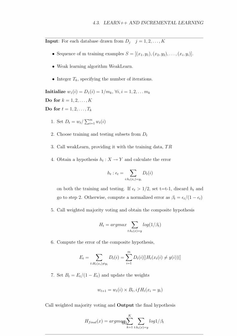
4.3. LEARN++ AND INCREMENTAL LEARNING
Input: For each database drawn from Dj j = 1, 2, . . . , K
• Sequence of m training examples S = [(x1, y1), (x2, y2), . . . , (xi, yi)].
• Weak learning algorithm WeakLearn.
• Integer Tk, specifying the number of iterations.
Initialize w1(i) = D1(i) = 1/mk, ∀i, i = 1, 2, . . . mk
Do for k = 1, 2, . . . , K
Do for t = 1, 2, . . . , Tk
1. Set Dt = wt/∑m
i=1 wt(i)
2. Choose training and testing subsets from Dt
3. Call weakLearn, providing it with the training data, TR
4. Obtain a hypothesis ht : X → Y and calculate the error
ht : εt =∑
i:ht(xi)=yi
Dt(i)
on both the training and testing. If εt > 1/2, set t=t-1, discard ht and
go to step 2. Otherwise, compute a normalized error as βt = εt/(1− εt)
5. Call weighted majority voting and obtain the composite hypothesis
Ht = argmax∑
t:ht(x)=y
log(1/βt)
6. Compute the error of the composite hypothesis,
Et =∑
t:Ht(xi) 6=yi
Dt(i) =m∑
i=1
Dt(i)[|Ht(xt(i) 6= y(i))|]
7. Set Bt = Et/(1− Et) and update the weights
wt+1 = wt(i)×Bt, ifHt(xi = yi)
Call weighted majority voting and Output the final hypothesis
Hfinal(x) = argmax
K∑k=1
∑t:ht(x)=y
log1/βt
Figure 4.6: The Learn++ algorithm
60
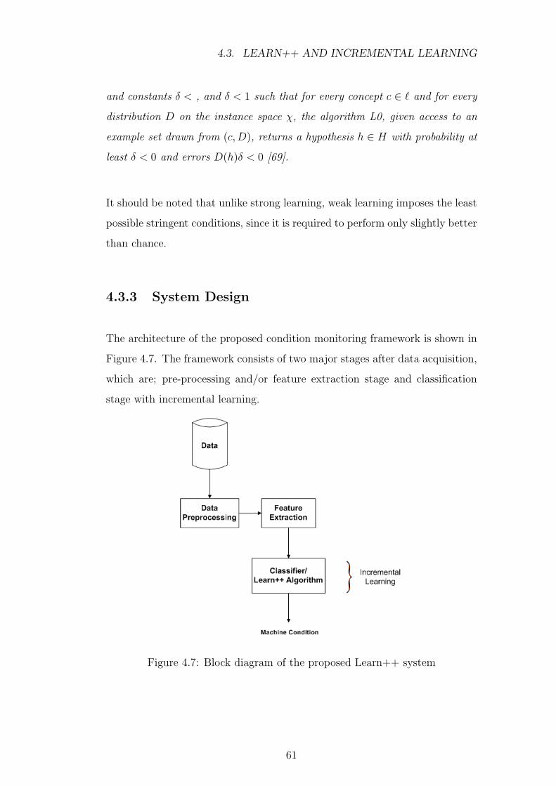
4.3. LEARN++ AND INCREMENTAL LEARNING
and constants δ < , and δ < 1 such that for every concept c ∈ ` and for every
distribution D on the instance space χ, the algorithm L0, given access to an
example set drawn from (c, D), returns a hypothesis h ∈ H with probability at
least δ < 0 and errors D(h)δ < 0 [69].
It should be noted that unlike strong learning, weak learning imposes the least
possible stringent conditions, since it is required to perform only slightly better
than chance.
4.3.3 System Design
The architecture of the proposed condition monitoring framework is shown in
Figure 4.7. The framework consists of two major stages after data acquisition,
which are; pre-processing and/or feature extraction stage and classification
stage with incremental learning.
Figure 4.7: Block diagram of the proposed Learn++ system
61
4.3. LEARN++ AND INCREMENTAL LEARNING
4.3.4 Experimental Results and Discussion
Experimentation is performed on two condition monitoring data set, the first
data is the Dissolved Gas Analysis from the high voltage bushing and the sec-
ond data set is the vibration data obtained from bearing. Three experiments
are performed to evaluate the effectiveness of Learn++. The first experiment
evaluates the incremental capability of the algorithm. This is done by eval-
uating the performance of Learn++ as new data is introduced. The second
experiment is performed to evaluate how well Learn++ can accommodate new
classes. The last experiment compares the performance of Learn++ with that
of a batch trained MLP. This is done to compare the classification rate of
Learn++ with that of a strong learner. The format of the tables in the fol-
lowing section was adopted from [8].
Bushing Data
First, the ten variables from the DGA data undergo a min-max normalization.
The normalization is a requirement for training an MLP as it ensure that the
data lies within similar range. Normalization is done using equation 4.1.
For the first experiment, the training data was divided into four databases each
with 300 training instances. In each training session, Learn++ is provided with
each database and generates 12 classifiers. The base Learner uses an MLP with
30 hidden layer neurons and 100 training cycles. To ensure that the method
retains previously seen data, for each training session, the previous database
is tested. Table 4.13 presents the results in which first four rows indicates
the classification performance of Learn++ on each of the databases after each
training session while the last row show the generalization capability on the
testing data. This demonstrates the performance improvement of Learn++
as inherited from AdaBoost on a single database. Table 4.13 further shows
that classifiers performances on the testing dataset, gradually improved from
62
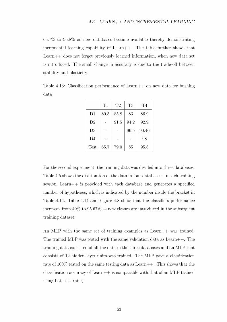
4.3. LEARN++ AND INCREMENTAL LEARNING
65.7% to 95.8% as new databases become available thereby demonstrating
incremental learning capability of Learn++. The table further shows that
Learn++ does not forget previously learned information, when new data set
is introduced. The small change in accuracy is due to the trade-off between
stability and plasticity.
Table 4.13: Classification performance of Learn++ on new data for bushing
data
T1 T2 T3 T4
D1 89.5 85.8 83 86.9
D2 - 91.5 94.2 92.9
D3 - - 96.5 90.46
D4 - - - 98
Test 65.7 79.0 85 95.8
For the second experiment, the training data was divided into three databases.
Table 4.5 shows the distribution of the data in four databases. In each training
session, Learn++ is provided with each database and generates a specified
number of hypotheses, which is indicated by the number inside the bracket in
Table 4.14. Table 4.14 and Figure 4.8 show that the classifiers performance
increases from 49% to 95.67% as new classes are introduced in the subsequent
training dataset.
An MLP with the same set of training examples as Learn++ was trained.
The trained MLP was tested with the same validation data as Learn++. The
training data consisted of all the data in the three databases and an MLP that
consists of 12 hidden layer units was trained. The MLP gave a classification
rate of 100% tested on the same testing data as Learn++. This shows that the
classification accuracy of Learn++ is comparable with that of an MLP trained
using batch learning.
63
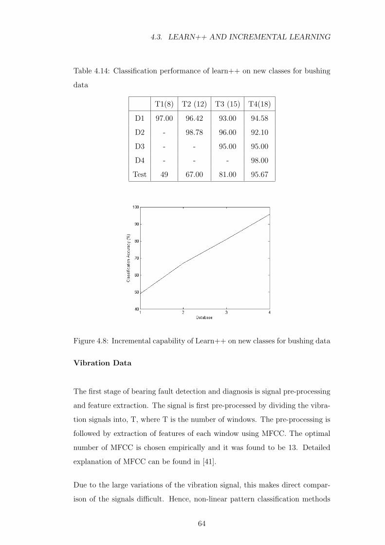
4.3. LEARN++ AND INCREMENTAL LEARNING
Table 4.14: Classification performance of learn++ on new classes for bushing
data
T1(8) T2 (12) T3 (15) T4(18)
D1 97.00 96.42 93.00 94.58
D2 - 98.78 96.00 92.10
D3 - - 95.00 95.00
D4 - - - 98.00
Test 49 67.00 81.00 95.67
Figure 4.8: Incremental capability of Learn++ on new classes for bushing data
Vibration Data
The first stage of bearing fault detection and diagnosis is signal pre-processing
and feature extraction. The signal is first pre-processed by dividing the vibra-
tion signals into, T, where T is the number of windows. The pre-processing is
followed by extraction of features of each window using MFCC. The optimal
number of MFCC is chosen empirically and it was found to be 13. Detailed
explanation of MFCC can be found in [41].
Due to the large variations of the vibration signal, this makes direct compar-
ison of the signals difficult. Hence, non-linear pattern classification methods
64
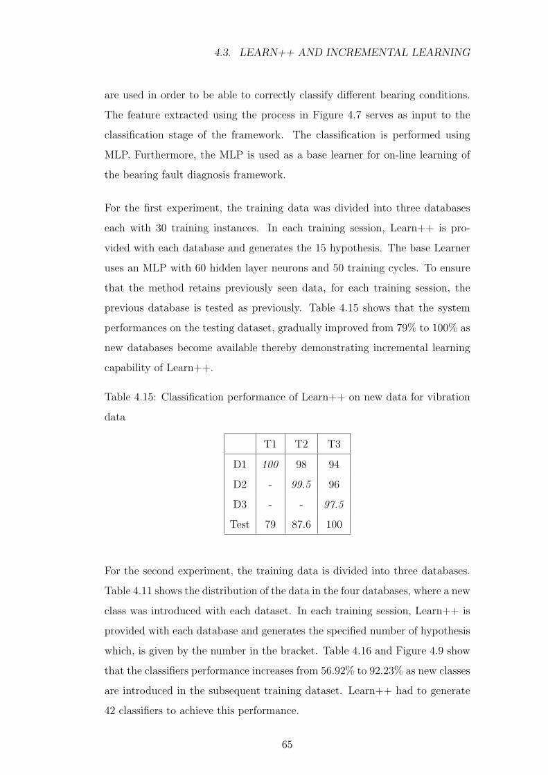
4.3. LEARN++ AND INCREMENTAL LEARNING
are used in order to be able to correctly classify different bearing conditions.
The feature extracted using the process in Figure 4.7 serves as input to the
classification stage of the framework. The classification is performed using
MLP. Furthermore, the MLP is used as a base learner for on-line learning of
the bearing fault diagnosis framework.
For the first experiment, the training data was divided into three databases
each with 30 training instances. In each training session, Learn++ is pro-
vided with each database and generates the 15 hypothesis. The base Learner
uses an MLP with 60 hidden layer neurons and 50 training cycles. To ensure
that the method retains previously seen data, for each training session, the
previous database is tested as previously. Table 4.15 shows that the system
performances on the testing dataset, gradually improved from 79% to 100% as
new databases become available thereby demonstrating incremental learning
capability of Learn++.
Table 4.15: Classification performance of Learn++ on new data for vibration
data
T1 T2 T3
D1 100 98 94
D2 - 99.5 96
D3 - - 97.5
Test 79 87.6 100
For the second experiment, the training data is divided into three databases.
Table 4.11 shows the distribution of the data in the four databases, where a new
class was introduced with each dataset. In each training session, Learn++ is
provided with each database and generates the specified number of hypothesis
which, is given by the number in the bracket. Table 4.16 and Figure 4.9 show
that the classifiers performance increases from 56.92% to 92.23% as new classes
are introduced in the subsequent training dataset. Learn++ had to generate
42 classifiers to achieve this performance.
65
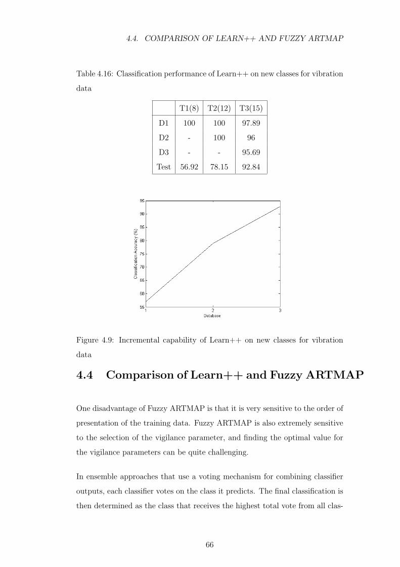
4.4. COMPARISON OF LEARN++ AND FUZZY ARTMAP
Table 4.16: Classification performance of Learn++ on new classes for vibration
data
T1(8) T2(12) T3(15)
D1 100 100 97.89
D2 - 100 96
D3 - - 95.69
Test 56.92 78.15 92.84
Figure 4.9: Incremental capability of Learn++ on new classes for vibration
data
4.4 Comparison of Learn++ and Fuzzy ARTMAP
One disadvantage of Fuzzy ARTMAP is that it is very sensitive to the order of
presentation of the training data. Fuzzy ARTMAP is also extremely sensitive
to the selection of the vigilance parameter, and finding the optimal value for
the vigilance parameters can be quite challenging.
In ensemble approaches that use a voting mechanism for combining classifier
outputs, each classifier votes on the class it predicts. The final classification is
then determined as the class that receives the highest total vote from all clas-
66
4.5. SUMMARY
sifiers. Learn++ uses weighted majority voting, where each classifier receives
a voting weight based on its training performance. This works well in practice
for most applications. However, for incremental learning problems that involve
introduction of new classes, the voting scheme proves to be unfair towards the
newly introduced class. Since none of the previously generated classifiers can
pick the new class, a relatively large number of new classifiers that recognize
the new class are needed, so that their total weight can out-vote the first batch
of classifiers on instances of the new class. This in return populates the en-
semble with an unnecessarily large number of classifiers. When incrementing
the system with new classes, it is best to ensure that the number of classifiers
that is added to the system is greater than the number of classifiers added
during a previous system increment. It is also better to include some data
from classes that have previously been seen. This ensures that if any pattern
is classified into one of the new classes, the votes from the previous classifiers
do not ‘outvote’ votes received from new classifiers. The major disadvantage
of Learn++ is that it is computationally expensive. Generally, to allow incre-
mental learning of the classes, classifiers had to be generated for the system,
while the same performance was obtained from a single classifier trained in
batch mode.
4.5 Summary
Current condition monitoring techniques provide promising results but lack
the incremental learning capability that will enable them to be used for au-
tomatic and continuous on-line monitoring. In this chapter, two incremental
learning algorithms were implemented and compared with each other. The
first algorithm uses fuzzy ARTMAP and the second algorithm uses Learn++.
The performance of the two algorithm is very comparable, however, the main
disadvantage of Learn++ is that it is computationally expensive and FAM is
sensitive to the selection of the vigilance parameter.
67

Chapter 5
A Multi-Agent System for
Condition Monitoring
Engineers have introduced better decision support systems for condition mon-
itoring procedures through applications of centralized intelligent systems by
using a variety of artificial intelligence (AI) techniques [7]. It is now widely rec-
ognized that problems due to the complexity of condition monitoring systems
can be overcome with architectures that contain many dynamically interacting
intelligent distributed modules, called intelligent agents [9]. Each agent is an
autonomous system, which processes as a selection of input, and the complete
interpretation and diagnosis is accomplished through interaction with other
agents. This chapter also looks at the advantages of using multi-agent tech-
niques, and how they can be used for condition monitoring. The chapter also
presents the conceptual framework of the multi-agent system and describes the
analysis and design including the information flow between agents to replicate
the diagnostic tasks performed by the engineers.
68
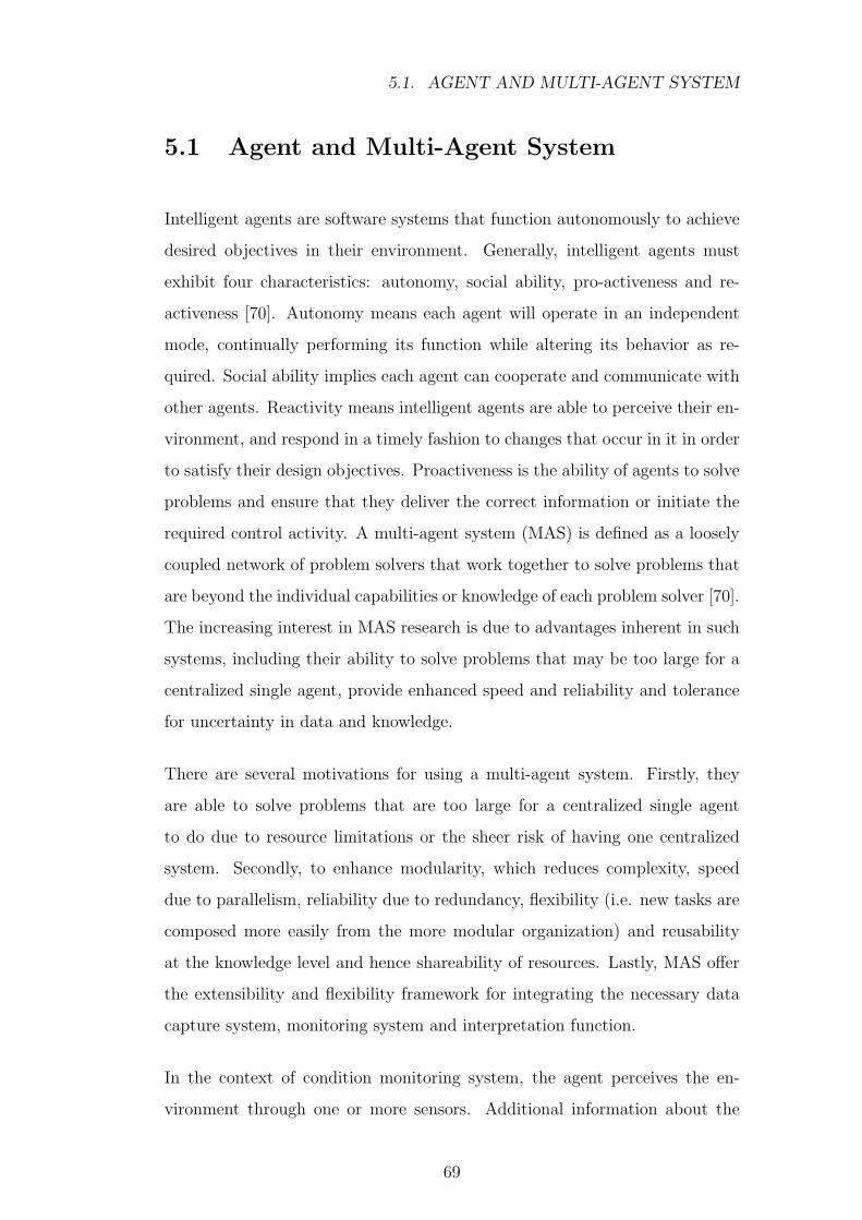
5.1. AGENT AND MULTI-AGENT SYSTEM
5.1 Agent and Multi-Agent System
Intelligent agents are software systems that function autonomously to achieve
desired objectives in their environment. Generally, intelligent agents must
exhibit four characteristics: autonomy, social ability, pro-activeness and re-
activeness [70]. Autonomy means each agent will operate in an independent
mode, continually performing its function while altering its behavior as re-
quired. Social ability implies each agent can cooperate and communicate with
other agents. Reactivity means intelligent agents are able to perceive their en-
vironment, and respond in a timely fashion to changes that occur in it in order
to satisfy their design objectives. Proactiveness is the ability of agents to solve
problems and ensure that they deliver the correct information or initiate the
required control activity. A multi-agent system (MAS) is defined as a loosely
coupled network of problem solvers that work together to solve problems that
are beyond the individual capabilities or knowledge of each problem solver [70].
The increasing interest in MAS research is due to advantages inherent in such
systems, including their ability to solve problems that may be too large for a
centralized single agent, provide enhanced speed and reliability and tolerance
for uncertainty in data and knowledge.
There are several motivations for using a multi-agent system. Firstly, they
are able to solve problems that are too large for a centralized single agent
to do due to resource limitations or the sheer risk of having one centralized
system. Secondly, to enhance modularity, which reduces complexity, speed
due to parallelism, reliability due to redundancy, flexibility (i.e. new tasks are
composed more easily from the more modular organization) and reusability
at the knowledge level and hence shareability of resources. Lastly, MAS offer
the extensibility and flexibility framework for integrating the necessary data
capture system, monitoring system and interpretation function.
In the context of condition monitoring system, the agent perceives the en-
vironment through one or more sensors. Additional information about the
69
5.2. POTENTIAL OF MAS
environment may also be acquired through communication with other agents
or systems. An agent’s ability to influence its environment may in the con-
text of condition monitoring be to operate a switch or adjust a process. An
action may also be to communicate with some other agents or human, e.g. a
technician close by and ask for help to carry out some preventive or corrective
needs.
Figure 5.1: Example of an agent
5.2 Potential of MAS
Multi-agent systems have proven to be an effective paradigm in a number of
distributed networked applications that require information integration from
multiple heterogeneous autonomous entities. More recently, MAS have be-
gun to emerge as an integrated solution approach to distributed computing,
communication, and data integration needs in industry.
5.2.1 Agent-based Computing and Agent-oriented Pro-
gramming
A multi-agent system consisting of multiple agents can take advantage of com-
putational resources and capabilities that are distributed across a network of
interconnected entities. An agent-based approach allows for the creation of
70
5.2. POTENTIAL OF MAS
systems that are flexible, robust, and can adapt to the environment [70]. This
is especially helpful when components of the system are not known in advance,
change over time, and are highly heterogeneous. Agent-based computing of-
fers the ability to decentralize computing solutions by incorporating auton-
omy and intelligence into cooperative, distributed applications. Each agent
perceives the state of its environment, infers by updating its internal knowl-
edge according to the newly received perceptions, decides on an action, and
acts to change the state of the environment. Agent-oriented programming is a
software paradigm used to facilitate agent-based computing and extends from
object-oriented programming by replacing the notions of class and inheritance
with the notions of roles and messages, respectively [70].
5.2.2 Knowledge-level Communication Capability
Within a multi-agent system, agents can communicate with each other using
agent communication languages, which resemble human-like speech actions
more than typical symbol-level program-to-program communication protocols
[70]. This capability enables agents to distill useful knowledge from volumi-
nous heterogeneous information sources and communicate with each other on
the basis of which they coordinate their actions. By enabling performance of
computation where computing resources and data are located, and allowing for
flexible communication of relevant results to relevant entities as needed, MAS
offer significant new capabilities to power systems, which have for so long de-
pended on various forms of expensive telemetry to satisfy most communication
needs.
5.2.3 Distributed Data Access and Processing
Another benefit offered by MAS is the distribution of agents across a net-
work [70]. Software agents may have different levels of intelligence, ranging
71
5.3. FUNCTIONAL DESIGN
from data agents and functional agents to decision agents. Because each agent
is designed to perform a specific role, with associated knowledge and skills,
distributed and heterogeneous information may be efficiently assimilated lo-
cally and utilized in a coordinated fashion in distributed knowledge networks,
resulting in reduced information processing time and network bandwidth in
comparison to that of more traditional centralized schemes.
5.2.4 Distributed Decision Support
MAS also offers a powerful task decomposition approach to problem solving
through interaction among agents. This is facilitated by the ability of different
agents to coordinate behavior through cooperation by agents establishing mu-
tually agreeable objectives, negotiation by agents negotiating until agreement
is reached, or mediation by agents resolving conflicts that cannot be resolved
by appealing to a third, neutral agent [71].
5.3 Functional Design
The requirements of condition monitoring outlined in Chapter 2 lead to the de-
sign of the condition monitoring system where functional modules are grouped
by their overall goal. A hierarchical layer was used due the flow of data from
one layer to another. The condition monitoring system consists of four layers;
• Data Monitoring Layer
• Interpretation Layer
• Diagnostic Layer
• Information Layer
72
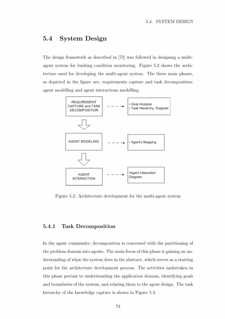
5.4. SYSTEM DESIGN
5.4 System Design
The design framework as described in [72] was followed in designing a multi-
agent system for bushing condition monitoring. Figure 5.2 shows the archi-
tecture used for developing the multi-agent system. The three main phases,
as depicted in the figure are; requirements capture and task decomposition;
agent modelling and agent interactions modelling.
Figure 5.2: Architecture development for the multi-agent system
5.4.1 Task Decomposition
In the agent community; decomposition is concerned with the partitioning of
the problem domain into agents. The main focus of this phase is gaining an un-
derstanding of what the system does in the abstract, which serves as a starting
point for the architecture development process. The activities undertaken in
this phase pertain to understanding the application domain, identifying goals
and boundaries of the system, and relating them to the agent design. The task
hierarchy of the knowledge capture is shown in Figure 5.3.
73
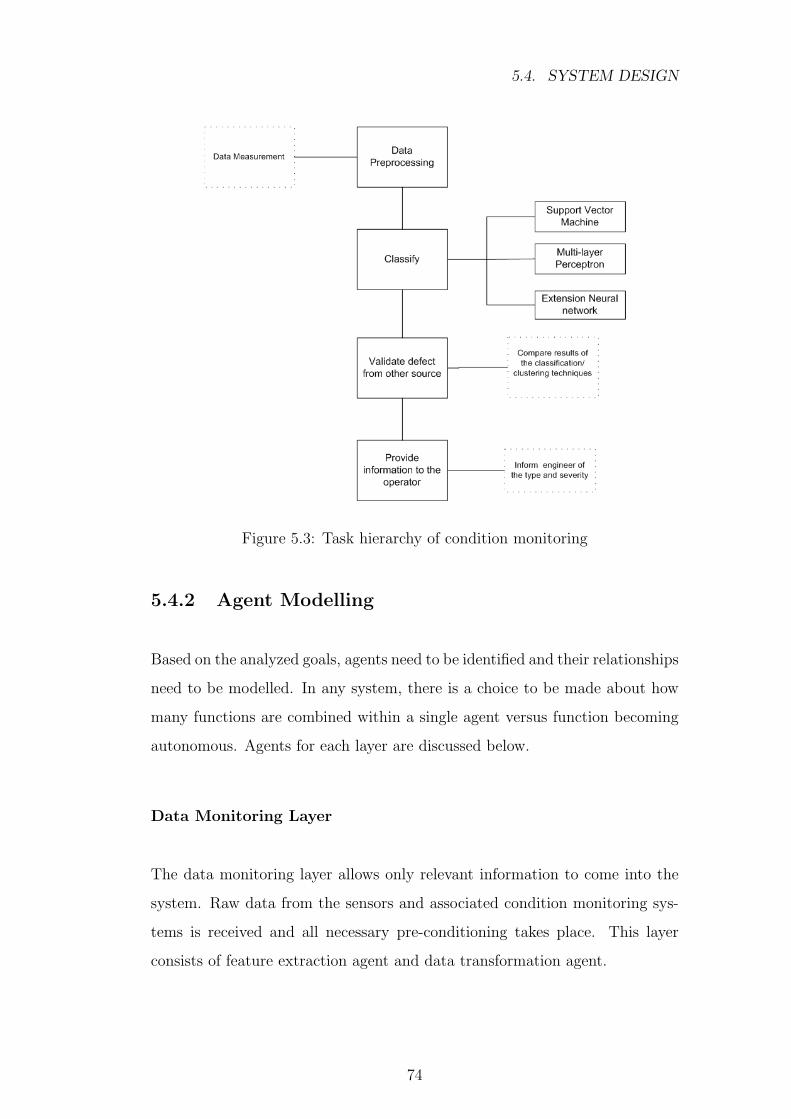
5.4. SYSTEM DESIGN
Figure 5.3: Task hierarchy of condition monitoring
5.4.2 Agent Modelling
Based on the analyzed goals, agents need to be identified and their relationships
need to be modelled. In any system, there is a choice to be made about how
many functions are combined within a single agent versus function becoming
autonomous. Agents for each layer are discussed below.
Data Monitoring Layer
The data monitoring layer allows only relevant information to come into the
system. Raw data from the sensors and associated condition monitoring sys-
tems is received and all necessary pre-conditioning takes place. This layer
consists of feature extraction agent and data transformation agent.
74
5.4. SYSTEM DESIGN
Feature Extraction Agent The feature extraction agent was designed to
provide the necessary data to the interpretation agents. Many parameters
may be used to characterize the conditions of the machine. Basic statistical
parameters are used to form the feature vector, providing some indication of
the shape (cross-correlation), symmetry (skew), peakedness (kurtosis) of the
vibration signal, effectively producing the fingerprint of the vibration signal.
The feature vector consists of parameter capable of differentiation between
different faults. Also MFCC features are used.
Data Transformation Agent The data preprocessing agent was designed
to provide the necessary conditioned data to the interpretation layer agents.
Data conditioning is an integral part of neural network architectures as it
makes it easier for the network to learn. There are cases where, one or two
variables are missing due to sensor failure. To accommodate inputs with miss-
ing variable, a zero imputation method is used. Markey et al. [73] showed
that this method is effective in replacing missing variable. The main reason
for retaining these blank entries is to ensure that no information about other
dissolved gases that may still give some information about the condition of the
equipment is lost. Secondly, data is normalized, this is done using the min-max
normalization. The equation for a min-max normalization for a single feature
is given by equation 4.1.
Interpretation Layer
The interpretation layer turns the data into information that can be easily
interpreted by plant operator. This module uses advanced intelligent sys-
tem techniques, coupled with codified knowledge and expertise in the area of
condition monitoring and to diagnose a problem. It supports more that one
interpretation technique. Data interpretation is achieved through three agents,
kernel-based classifier, backpropagation neural network, and extension neural
network.
75
5.4. SYSTEM DESIGN
Diagnostics Layer
The diagnostic layer consists of two diagnosis agents, that are allowed to shared
information and compare their decision.
Diagnostic Agent This agent takes the outputs of the interpretation layer
agents and builds an overall diagnostic conclusion. It is known that the per-
formance of ensemble is often much better than that of individual classifiers,
because of independently-trained classifiers and their uncorrelated errors [54].
Since several independent agent classifiers are used, we need to aggregate them
in an appropriate manner. A number of decision fusion techniques exist such
as weighted majority voting, majority voting and trained combiner fusion. The
majority voting is the simplest and widely-used aggregation method [54]. This
voting scheme treats all agents with equal weights. Prediction errors of agent
are often different, thus, it is more reasonable to give them different weights, in
proportion to their prediction performance. In the weighted majority voting,
the predicted class label of the diagnosis agent is given by;
Cm = argmaxK∑
k=1
W (k, m)Ikm (5.1)
Where W(k,m) is the weight when the predicted class label of the kth agent is
Cm. The weights can be determined by calculating appropriate performance
measures for each classifier as mentioned in previous sections. The weights of
the classifiers must add up to one. A table is built with classifier tabulated
against conclusion, the cell data is then populated with various results that
have been submitted to the diagnosis agent. Each time new results are added,
the conclusion is recalculated. After the table is fully populated, the weighted
majority voting is used to determine an outcome of the event.
76
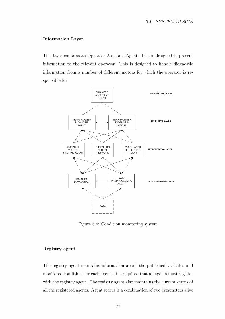
5.4. SYSTEM DESIGN
Information Layer
This layer contains an Operator Assistant Agent. This is designed to present
information to the relevant operator. This is designed to handle diagnostic
information from a number of different motors for which the operator is re-
sponsible for.
Figure 5.4: Condition monitoring system
Registry agent
The registry agent maintains information about the published variables and
monitored conditions for each agent. It is required that all agents must register
with the registry agent. The registry agent also maintains the current status of
all the registered agents. Agent status is a combination of two parameters alive
77
5.4. SYSTEM DESIGN
and reachable. The status of a communication link between any two agents is
determined by attempting to achieve a reliable communication between them.
The registry agent is used to find information about agents who may supply
required data.
5.4.3 Agent Interaction
Agent interaction defines communications and exchange of information be-
tween different agents. Agent-based systems require a communication infras-
tructure. Agents in the condition monitoring system communicate with each
other by sending messages in the Agent Communication Language specified
by FIPA [74]. Agent interaction is facilitated by the registry agent using sub-
scribes, query, inform and confirm command. These messages correspond to
registration requests, information requests and other agent actions. A brief
overview of agent actions and the corresponding messages is given below.
Registration of an agent with the registry agent : Each agent must register
with the registry agent. A registration message includes the registering agent’s
agent-id, list of published variables. The registry agent issues a confirmation
message upon successfully entering the new agent in its database.
Information request by an agent about other agents : To find agents capable of
providing required input data, the agent sends a search request to the agent
registry. The search request includes the requester’s agent-id, and the required
variables.
Registry agent’s reply to an information request : Upon receiving a search re-
quest, the registry agent verifies that the request is legitimate before searching
its database to determine which agents can supply the requested variables and
the status of these agents. The message from the registry agent to the requester
includes the requested variable name, the agent-id of the agent publishing the
variable and the status of the requested agent.
Request for belief subscription: Upon receiving the list of agents capable of
providing the required input from the registry, the subscribing agent sends
78
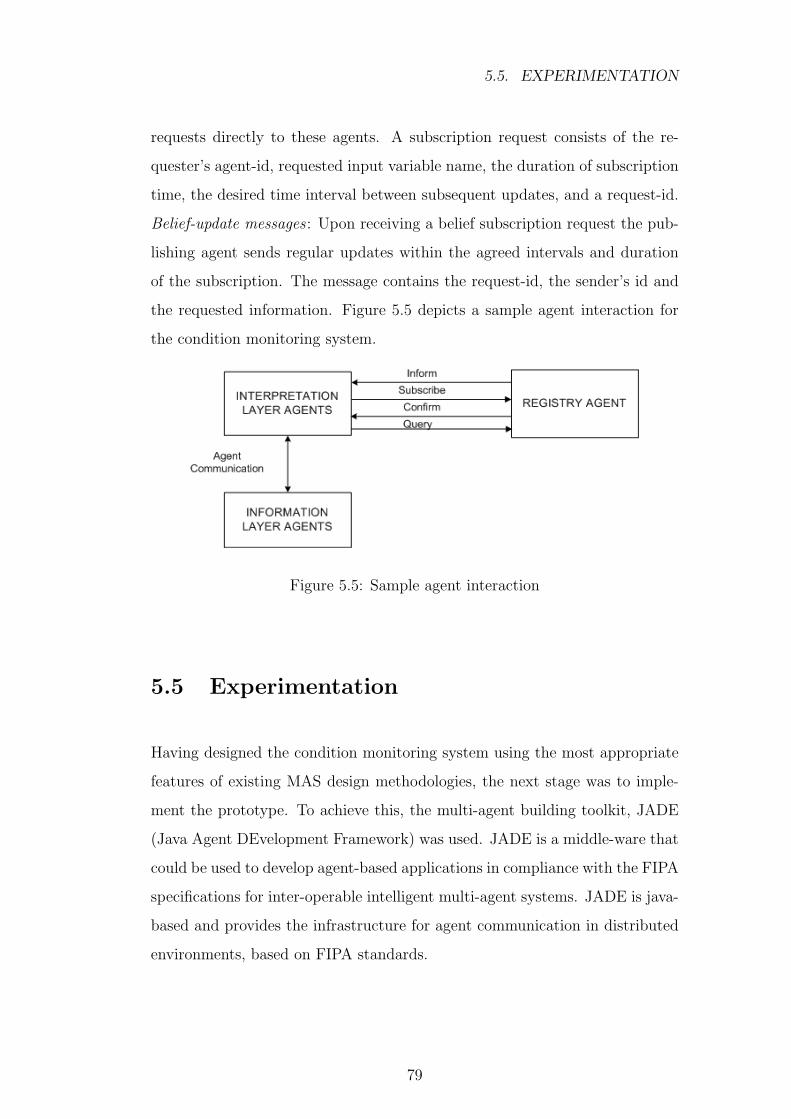
5.5. EXPERIMENTATION
requests directly to these agents. A subscription request consists of the re-
quester’s agent-id, requested input variable name, the duration of subscription
time, the desired time interval between subsequent updates, and a request-id.
Belief-update messages : Upon receiving a belief subscription request the pub-
lishing agent sends regular updates within the agreed intervals and duration
of the subscription. The message contains the request-id, the sender’s id and
the requested information. Figure 5.5 depicts a sample agent interaction for
the condition monitoring system.
Figure 5.5: Sample agent interaction
5.5 Experimentation
Having designed the condition monitoring system using the most appropriate
features of existing MAS design methodologies, the next stage was to imple-
ment the prototype. To achieve this, the multi-agent building toolkit, JADE
(Java Agent DEvelopment Framework) was used. JADE is a middle-ware that
could be used to develop agent-based applications in compliance with the FIPA
specifications for inter-operable intelligent multi-agent systems. JADE is java-
based and provides the infrastructure for agent communication in distributed
environments, based on FIPA standards.
79
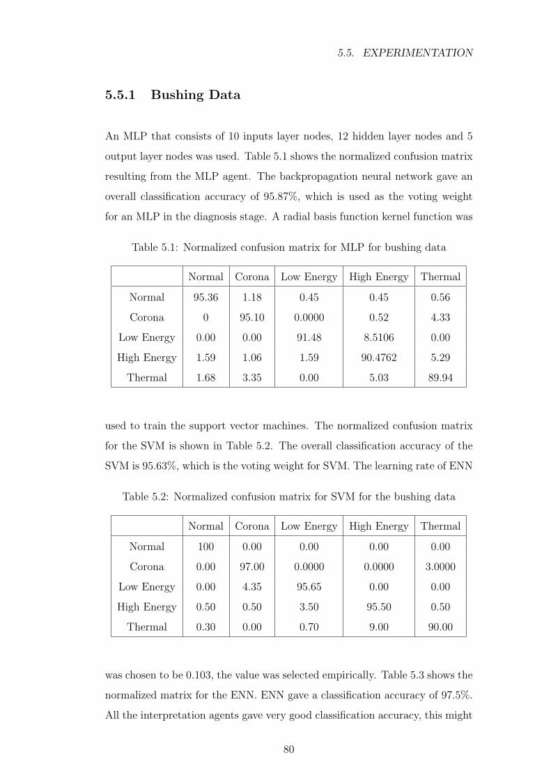
5.5. EXPERIMENTATION
5.5.1 Bushing Data
An MLP that consists of 10 inputs layer nodes, 12 hidden layer nodes and 5
output layer nodes was used. Table 5.1 shows the normalized confusion matrix
resulting from the MLP agent. The backpropagation neural network gave an
overall classification accuracy of 95.87%, which is used as the voting weight
for an MLP in the diagnosis stage. A radial basis function kernel function was
Table 5.1: Normalized confusion matrix for MLP for bushing data
Normal Corona Low Energy High Energy Thermal
Normal 95.36 1.18 0.45 0.45 0.56
Corona 0 95.10 0.0000 0.52 4.33
Low Energy 0.00 0.00 91.48 8.5106 0.00
High Energy 1.59 1.06 1.59 90.4762 5.29
Thermal 1.68 3.35 0.00 5.03 89.94
used to train the support vector machines. The normalized confusion matrix
for the SVM is shown in Table 5.2. The overall classification accuracy of the
SVM is 95.63%, which is the voting weight for SVM. The learning rate of ENN
Table 5.2: Normalized confusion matrix for SVM for the bushing data
Normal Corona Low Energy High Energy Thermal
Normal 100 0.00 0.00 0.00 0.00
Corona 0.00 97.00 0.0000 0.0000 3.0000
Low Energy 0.00 4.35 95.65 0.00 0.00
High Energy 0.50 0.50 3.50 95.50 0.50
Thermal 0.30 0.00 0.70 9.00 90.00
was chosen to be 0.103, the value was selected empirically. Table 5.3 shows the
normalized matrix for the ENN. ENN gave a classification accuracy of 97.5%.
All the interpretation agents gave very good classification accuracy, this might
80
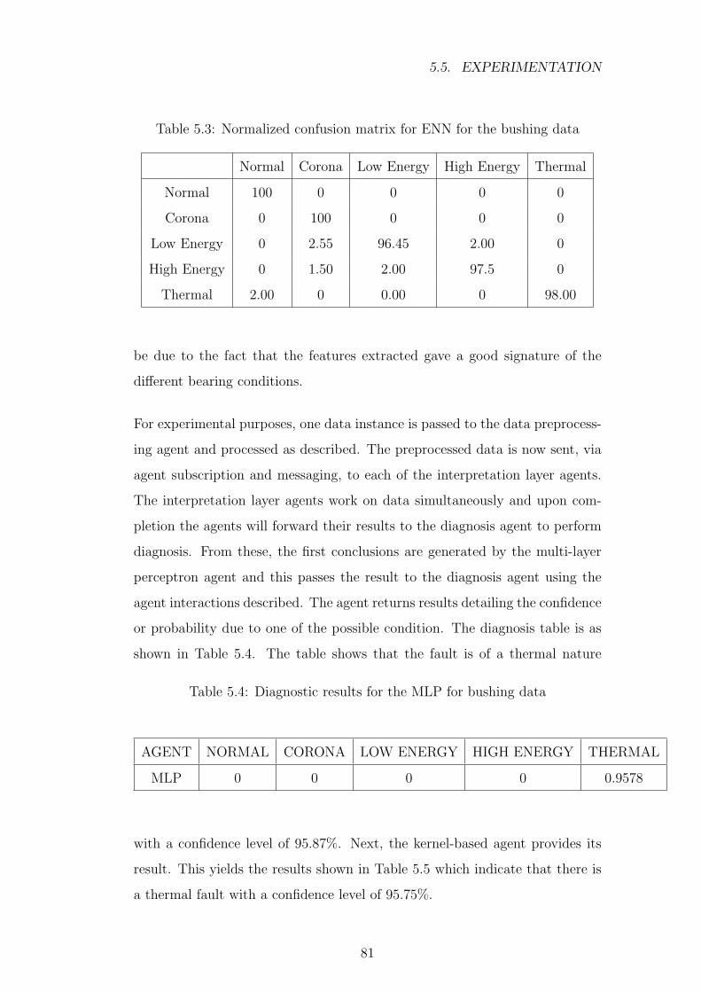
5.5. EXPERIMENTATION
Table 5.3: Normalized confusion matrix for ENN for the bushing data
Normal Corona Low Energy High Energy Thermal
Normal 100 0 0 0 0
Corona 0 100 0 0 0
Low Energy 0 2.55 96.45 2.00 0
High Energy 0 1.50 2.00 97.5 0
Thermal 2.00 0 0.00 0 98.00
be due to the fact that the features extracted gave a good signature of the
different bearing conditions.
For experimental purposes, one data instance is passed to the data preprocess-
ing agent and processed as described. The preprocessed data is now sent, via
agent subscription and messaging, to each of the interpretation layer agents.
The interpretation layer agents work on data simultaneously and upon com-
pletion the agents will forward their results to the diagnosis agent to perform
diagnosis. From these, the first conclusions are generated by the multi-layer
perceptron agent and this passes the result to the diagnosis agent using the
agent interactions described. The agent returns results detailing the confidence
or probability due to one of the possible condition. The diagnosis table is as
shown in Table 5.4. The table shows that the fault is of a thermal nature
Table 5.4: Diagnostic results for the MLP for bushing data
AGENT NORMAL CORONA LOW ENERGY HIGH ENERGY THERMAL
MLP 0 0 0 0 0.9578
with a confidence level of 95.87%. Next, the kernel-based agent provides its
result. This yields the results shown in Table 5.5 which indicate that there is
a thermal fault with a confidence level of 95.75%.
81
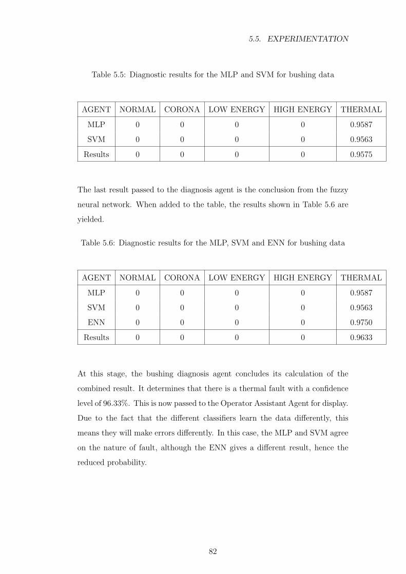
5.5. EXPERIMENTATION
Table 5.5: Diagnostic results for the MLP and SVM for bushing data
AGENT NORMAL CORONA LOW ENERGY HIGH ENERGY THERMAL
MLP 0 0 0 0 0.9587
SVM 0 0 0 0 0.9563
Results 0 0 0 0 0.9575
The last result passed to the diagnosis agent is the conclusion from the fuzzy
neural network. When added to the table, the results shown in Table 5.6 are
yielded.
Table 5.6: Diagnostic results for the MLP, SVM and ENN for bushing data
AGENT NORMAL CORONA LOW ENERGY HIGH ENERGY THERMAL
MLP 0 0 0 0 0.9587
SVM 0 0 0 0 0.9563
ENN 0 0 0 0 0.9750
Results 0 0 0 0 0.9633
At this stage, the bushing diagnosis agent concludes its calculation of the
combined result. It determines that there is a thermal fault with a confidence
level of 96.33%. This is now passed to the Operator Assistant Agent for display.
Due to the fact that the different classifiers learn the data differently, this
means they will make errors differently. In this case, the MLP and SVM agree
on the nature of fault, although the ENN gives a different result, hence the
reduced probability.
82
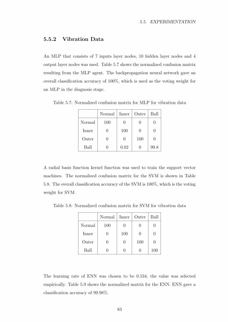
5.5. EXPERIMENTATION
5.5.2 Vibration Data
An MLP that consists of 7 inputs layer nodes, 10 hidden layer nodes and 4
output layer nodes was used. Table 5.7 shows the normalized confusion matrix
resulting from the MLP agent. The backpropagation neural network gave an
overall classification accuracy of 100%, which is used as the voting weight for
an MLP in the diagnosis stage.
Table 5.7: Normalized confusion matrix for MLP for vibration data
Normal Inner Outer Ball
Normal 100 0 0 0
Inner 0 100 0 0
Outer 0 0 100 0
Ball 0 0.02 0 99.8
A radial basis function kernel function was used to train the support vector
machines. The normalized confusion matrix for the SVM is shown in Table
5.8. The overall classification accuracy of the SVM is 100%, which is the voting
weight for SVM.
Table 5.8: Normalized confusion matrix for SVM for vibration data
Normal Inner Outer Ball
Normal 100 0 0 0
Inner 0 100 0 0
Outer 0 0 100 0
Ball 0 0 0 100
The learning rate of ENN was chosen to be 0.534, the value was selected
empirically. Table 5.9 shows the normalized matrix for the ENN. ENN gave a
classification accuracy of 99.98%.
83
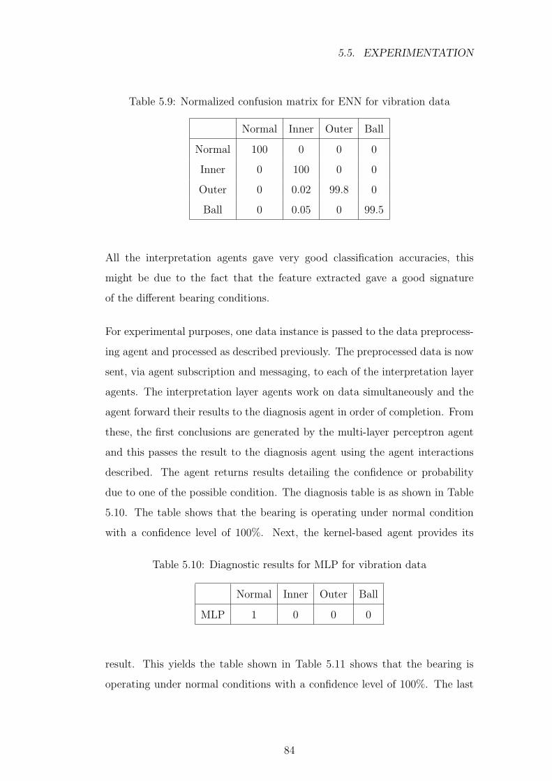
5.5. EXPERIMENTATION
Table 5.9: Normalized confusion matrix for ENN for vibration data
Normal Inner Outer Ball
Normal 100 0 0 0
Inner 0 100 0 0
Outer 0 0.02 99.8 0
Ball 0 0.05 0 99.5
All the interpretation agents gave very good classification accuracies, this
might be due to the fact that the feature extracted gave a good signature
of the different bearing conditions.
For experimental purposes, one data instance is passed to the data preprocess-
ing agent and processed as described previously. The preprocessed data is now
sent, via agent subscription and messaging, to each of the interpretation layer
agents. The interpretation layer agents work on data simultaneously and the
agent forward their results to the diagnosis agent in order of completion. From
these, the first conclusions are generated by the multi-layer perceptron agent
and this passes the result to the diagnosis agent using the agent interactions
described. The agent returns results detailing the confidence or probability
due to one of the possible condition. The diagnosis table is as shown in Table
5.10. The table shows that the bearing is operating under normal condition
with a confidence level of 100%. Next, the kernel-based agent provides its
Table 5.10: Diagnostic results for MLP for vibration data
Normal Inner Outer Ball
MLP 1 0 0 0
result. This yields the table shown in Table 5.11 shows that the bearing is
operating under normal conditions with a confidence level of 100%. The last
84
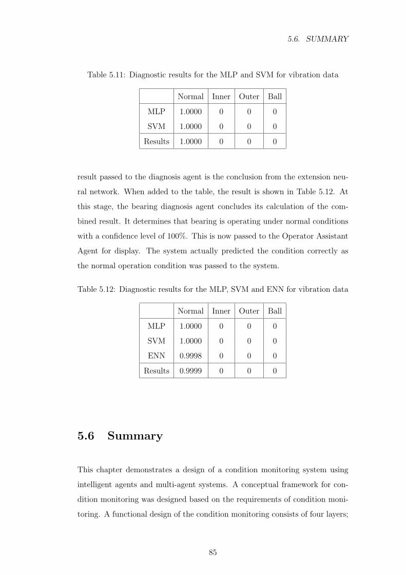
5.6. SUMMARY
Table 5.11: Diagnostic results for the MLP and SVM for vibration data
Normal Inner Outer Ball
MLP 1.0000 0 0 0
SVM 1.0000 0 0 0
Results 1.0000 0 0 0
result passed to the diagnosis agent is the conclusion from the extension neu-
ral network. When added to the table, the result is shown in Table 5.12. At
this stage, the bearing diagnosis agent concludes its calculation of the com-
bined result. It determines that bearing is operating under normal conditions
with a confidence level of 100%. This is now passed to the Operator Assistant
Agent for display. The system actually predicted the condition correctly as
the normal operation condition was passed to the system.
Table 5.12: Diagnostic results for the MLP, SVM and ENN for vibration data
Normal Inner Outer Ball
MLP 1.0000 0 0 0
SVM 1.0000 0 0 0
ENN 0.9998 0 0 0
Results 0.9999 0 0 0
5.6 Summary
This chapter demonstrates a design of a condition monitoring system using
intelligent agents and multi-agent systems. A conceptual framework for con-
dition monitoring was designed based on the requirements of condition moni-
toring. A functional design of the condition monitoring consists of four layers;
85

5.6. SUMMARY
the data monitoring layer, interpretation layer, diagnostic layer and informa-
tion layer, which were presented. The data monitoring layer consists of two
agents which are responsible for extracting features and conditioning of data
received from the measurement system. The interpretation layer consists of
three agents, the kernel-based agent, backpropagation agent and extension
neural network agent. The interpretation agents are encapsulated with classi-
fiers hence, were trained prior to usage. These agents interpret data from the
data monitoring layer and give a diagnosis on the condition of the equipment.
The diagnosis layer uses weighted majority voting to combine the decision
from the interpretation agents. This information along with the maintenance
recommendations are passed to the operator assistant agent.
The adoption of a distributed MAS architecture also provides a basis for con-
tinual improvement of engineering decision support due to the flexibility and
scalability achieved by the use of common communication mechanism. This
system will enable integration of further data sources and interpretation agents.
86
Chapter 6
Conclusion
6.1 Comparison of Classifiers
The fuzzy ARTMAP gave slightly better results than the MLP, SVM and
ENN classifiers. This might be due to the fact that the structure of the fuzzy
ARTMAP adapts, creating a larger number of categories in which to map the
output labels as the training data becomes available.
The ensemble of classifiers gave an improvement on the classification accuracy
from a single fuzzy ARTMAP. In the creation of the ensemble, the correlation
was used. It might be useful to compare various classifier selection techniques
such as the agreement and diversity measure to find a technique that gives
the best results. Also, it might be useful to investigate the effect of different
decision fusion systems for bushing condition monitoring.
6.2 Incremental Learning
The problem with batch learning is that if new information has to be added
to the classifier, for this involves discarding the existing classifier and training
87
6.3. MULTI-AGENT SYSTEM
a new classifier using accumulated data. Another method involves modifying
the weights of the classifier using the misclassified instances only. These meth-
ods suffer from catastrophic forgetting and they require access to old data and
require optimization of the training parameters. In the incremental learning
system, the old system can learn new information on-line without requiring
access to old data or forgetting previously learned information. Two incre-
mental learning algorithm were implemented. The first incremental learning
algorithm uses an ensemble of MLP classifier that are combined using the
weighted majority voting known as Learn++. The second algorithm uses the
fuzzy ARTMAP and to enhance the performance of a single FAM and an en-
semble of FAM, two different scenarios were considered. In the simplest case,
the systems were asked to learn from new data that did not include any new
class information, simply to improve its classification performance. In the
second case, the problem was made considerably more difficult by asking the
systems to learn patterns coming from a new class not encountered before.
Both the algorithm were able to accommodate both new data and new classes
without forgetting previously learned information. Both the algorithm were
able to accommodate both new data and new classes without forgetting pre-
viously learned information. However, the main disadvantage of the Learn++
is that it was computationally expensive and suffers from the problem of out-
voting. The main disadvantage of the FAM system is that it is very sensitive
to the selection of the vigilance parameter.
6.3 Multi-agent System
The work illustrates how a multi-agent system can be used to effectively in-
tegrate existing stand-alone intelligent systems and new interpretation ap-
proaches within an environment which offers long term flexibility and scalabil-
ity. This work has economic impact as the agent-based condition monitoring
system with the integrated tools for data classification and clustering, along
88
6.4. SUGGESTIONS FOR FUTURE RESEARCH
with the embedded artificial intelligence techniques and automated modelling
and simulation will enable the minimization capital investment and operat-
ing costs. This will be achieved by reducing process steps, predicting specific
problems and conditions under which the problems can occur and increas-
ing equipment utilization through better scheduling and understanding of the
problem domain.
6.4 Suggestions for Future Research
Future work should integrate various measurement data into the existing model.
Since, the agents function in a dynamic environment and they need to update
their knowledge as the environment changes, future work should look into in-
corporating the incremental learning system into the multi-agent system to
ensure that the agents are able to adapt. Learning in multi-agent system af-
fects the co-operation of agents, hence the effect of learning in this system
must also be studied. Also the scalability of the multi-agent system must also
be investigated.
89
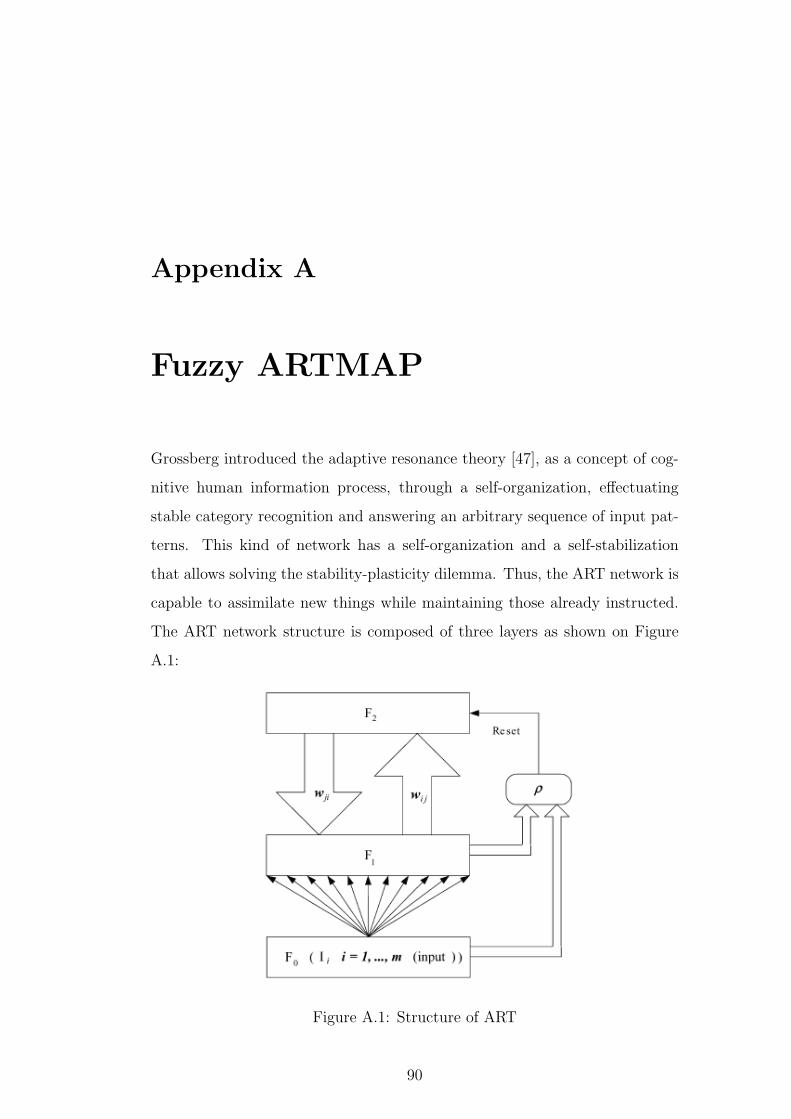
Appendix A
Fuzzy ARTMAP
Grossberg introduced the adaptive resonance theory [47], as a concept of cog-
nitive human information process, through a self-organization, effectuating
stable category recognition and answering an arbitrary sequence of input pat-
terns. This kind of network has a self-organization and a self-stabilization
that allows solving the stability-plasticity dilemma. Thus, the ART network is
capable to assimilate new things while maintaining those already instructed.
The ART network structure is composed of three layers as shown on Figure
A.1:
Figure A.1: Structure of ART
90
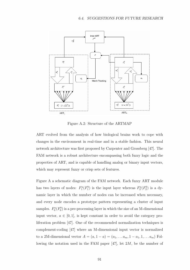
6.4. SUGGESTIONS FOR FUTURE RESEARCH
Figure A.2: Structure of the ARTMAP
ART evolved from the analysis of how biological brains work to cope with
changes in the environment in real-time and in a stable fashion. This neural
network architecture was first proposed by Carpenter and Grossberg [47]. The
FAM network is a robust architecture encompassing both fuzzy logic and the
properties of ART, and is capable of handling analog or binary input vectors,
which may represent fuzzy or crisp sets of features.
Figure A a schematic diagram of the FAM network. Each fuzzy ART module
has two layers of nodes: F a1 (F b
1 ) is the input layer whereas F a2 (F b
2 ) is a dy-
namic layer in which the number of nodes can be increased when necessary,
and every node encodes a prototype pattern representing a cluster of input
samples. F a0 (F b
0 ) is a pre-processing layer in which the size of an M-dimensional
input vector, a ∈ [0, 1], is kept constant in order to avoid the category pro-
liferation problem [47]. One of the recommended normalization techniques is
complement-coding [47] where an M-dimensional input vector is normalized
to a 2M-dimensional vector A = (a, 1 − a) = (a1, . . . am, 1 − a1, 1, . . . am) Fol-
lowing the notation used in the FAM paper [47], let 2M , be the number of
91
A.1. INITIALIZATION
nodes in F a1 and N , be the number of nodes in F a
2 . The Short Term Memory
traces or activity vectors of Fy and F ; are denoted by xa = (xa1, . . . , x
a2Ma
) and
ya = (ya1 , . . . , y
aNa
); and waj = (wa
j1, . . . , waj.2Ma
), j = 1, . . . , N , is the jth ART,
weight vector or the Long Term Memory trace. The same notation applies
to ARTb when the superscripts or subscripts a and b are interchanged. In
the map field, wabj = (wab
j1, . . . , wabjNa
), j = 1, . . . , N , is the weight vector from
the jth F b2 node to Fab, xab = (x1
ab, . . . , n) is the map field activity vector. In
general, the FAM algorithm can be divided into four phases:
A.1 Initialization
In a Fuzzy ART module, the weight vectors subsume both the bottom-up and
top-down weight vectors of ARTa [47]. In ART,, each category node weight
vector fans-out to all the nodes in the Fy layer. These weight vectors are
initialized to unity;
waj1 = . . . = wa
j.2Ma(0) = 1 j = 1, . . . , N, (A.1)
There are three parameters associated with ARTa and ARTb, namely the choice
parameter,ηa , the learning rate, β , and the baseline vigilance parameter, ρ.
To operate in the conservative mode where recoding during learning will be
minimized, ρ, should be initialized close to 0. The values of β, and η are
set between 0 and 1. The same initialization procedure is also applicable
to ARTb. In the map field, the vigilance parameter, ηab, is also initialized
between 0 and 1, whereas the weight vectors from F b2 to Fab are set to unity.
Note that the number of nodes in Fab is the same as the number of nodes in
F b2 , and there is a one-to-one permanent link between each corresponding pair
of nodes. Activities in Fuzzy ART. During supervised learning, ART, receives
an input vector, and ARTb receives the associated target vector. After pre-
processing, the complement-coded input vector A is propagated from F a1 to
F a2 ; through wa. A fuzzy choice function is used to measure the response of
92
A.1. INITIALIZATION
each F a2 prototype node as follows:
Tj(A) =A ∧ wa
j
αa + wjalj = 1, . . . , Na (A.2)
The fuzzy MIN operator (∧) and the size l.l are defined as: (x∧y) ≡ min(xi, yi)
and lxl =∑‖xi| [75]. The maximally responsive node is selected as the win-
ner, denoted as node J , while all other nodes are shutdown in accordance with
the winner-take-all competition. The winning node then sends its weight vec-
tor to F a1 , and a vigilance test is performed to compare the similarity between
the activity vector, xa, and the input vector against the vigilance parameter:
xa
A=
A ∧ waj
A≥ ρa (A.3)
where wj is the weight vector of the Jth winning node in F a2 . If this novelty
test is satisfied, resonance is said to occur, and learning takes place. However,
if the test fails, the winning node is inhibited, and A is retransmitted to to
search for a new winner which is able to fulfill the vigilance test. If such a
node does not exist, a new node is recruited to code the input vector. The
same search cycle for the target vector goes on simultaneously in ARTb where
a prototype node in F a2 : that best matches the target vector will be found.
In general, an independent Fuzzy ART module is employed as ARTb to self-
organize the target vectors. However, in one-from-N classification (i.e. each
input pattern belongs to only one of the N possible output classes), ARTb can
be replaced by a single layer containing N nodes. Then, the N-bit teaching
stimulus can be coded to have unit value corresponding to the target category
and zero for all others. Activities in the map field. The comparison between
F a2 and F b
2 ; activities takes place in the map field. If K is the winning node in
ARTb, then
ybk =
1 if j=J and k=K
0 otherwise(A.4)
93

A.2. MATCH TRACKING
Assuming that both ARTa, and ARTb are active, the Fab activity vector, xab,
obeys
xab = yb ∧ wabj (A.5)
which forms a prediction from the Jth ART, category to the Kth ARTb target
class via wabj . A map field vigilance test is performed to determine the similarity
between xab and yb against a user-defined map field vigilance parameter, ρab,
i.e.:|xab||yb|
≥ ρab (A.6)
If equation A.6 is satisfied, learning ensues in ART , ARTb and the map field
as defined in previous section. Conversely, if equation A.6 fails, an activity
called match tracking is triggered which initiates a new search cycle in ARTa,.
A.2 Match tracking
For each new input vector, the ART , vigilance parameter, ρa, equals a user-
defined baseline vigilance, ρa. In response to a failure in the map field vigilance
test, ρa is raised to
ρa =
∣∣A ∧ waj
∣∣|A|
+ δ (A.7)
Where δ is a small positive value slightly greater than zero. Thus, the ARTa,
vigilance test Equation A.7 fails, and a new winner in F a2 has to be selected.
In other words, match tracking provides a means to select a category node
which satisfies both the ARTa, and the map field vigilance tests. If no such
node exists, the current input vector will be ignored.
94
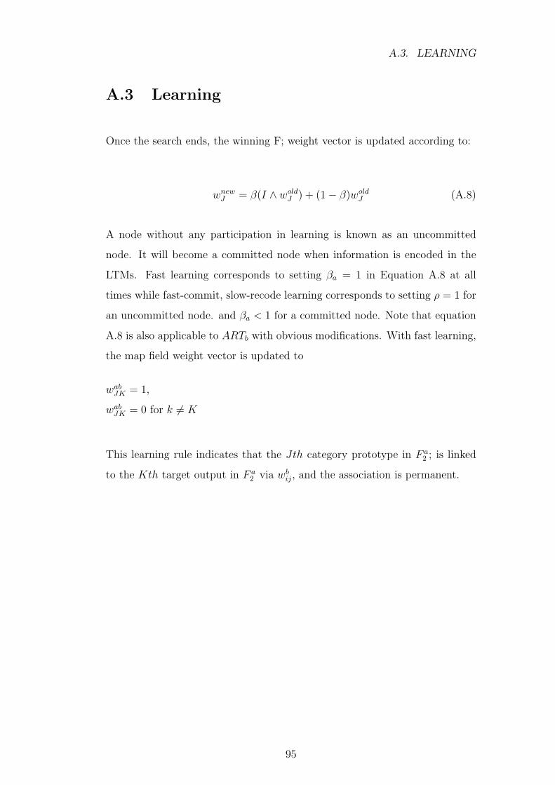
A.3. LEARNING
A.3 Learning
Once the search ends, the winning F; weight vector is updated according to:
wnewJ = β(I ∧ wold
J ) + (1− β)woldJ (A.8)
A node without any participation in learning is known as an uncommitted
node. It will become a committed node when information is encoded in the
LTMs. Fast learning corresponds to setting βa = 1 in Equation A.8 at all
times while fast-commit, slow-recode learning corresponds to setting ρ = 1 for
an uncommitted node. and βa < 1 for a committed node. Note that equation
A.8 is also applicable to ARTb with obvious modifications. With fast learning,
the map field weight vector is updated to
wabJK = 1,
wabJK = 0 for k 6= K
This learning rule indicates that the Jth category prototype in F a2 ; is linked
to the Kth target output in F a2 via wb
ij, and the association is permanent.
95
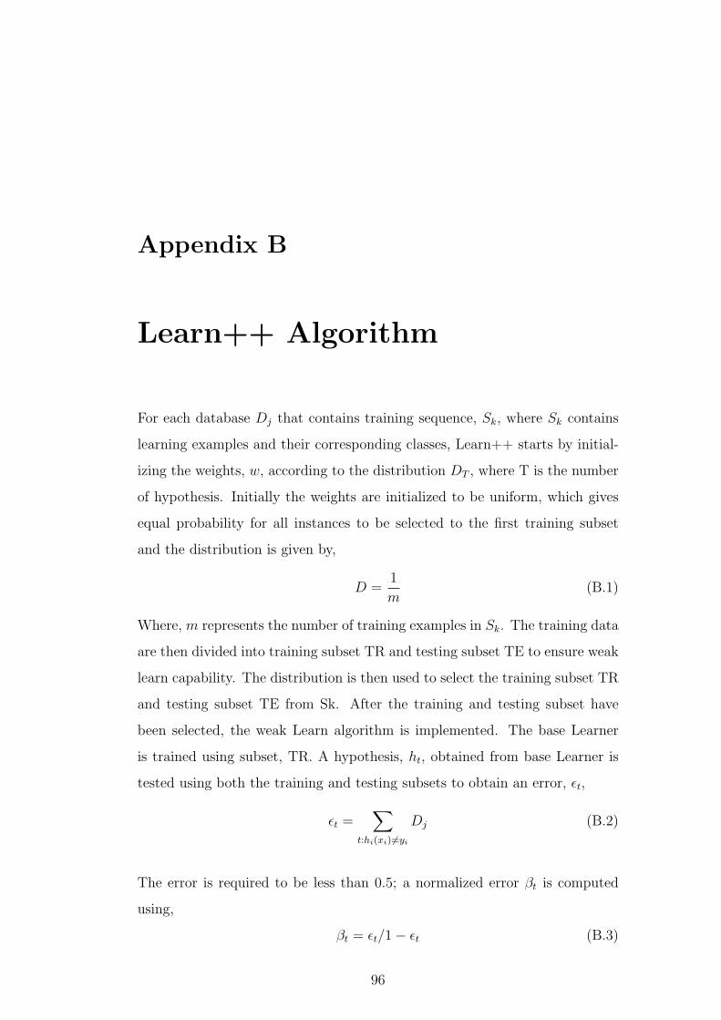
Appendix B
Learn++ Algorithm
For each database Dj that contains training sequence, Sk, where Sk contains
learning examples and their corresponding classes, Learn++ starts by initial-
izing the weights, w, according to the distribution DT , where T is the number
of hypothesis. Initially the weights are initialized to be uniform, which gives
equal probability for all instances to be selected to the first training subset
and the distribution is given by,
D =1
m(B.1)
Where, m represents the number of training examples in Sk. The training data
are then divided into training subset TR and testing subset TE to ensure weak
learn capability. The distribution is then used to select the training subset TR
and testing subset TE from Sk. After the training and testing subset have
been selected, the weak Learn algorithm is implemented. The base Learner
is trained using subset, TR. A hypothesis, ht, obtained from base Learner is
tested using both the training and testing subsets to obtain an error, εt,
εt =∑
t:hi(xi) 6=yi
Dj (B.2)
The error is required to be less than 0.5; a normalized error βt is computed
using,
βt = εt/1− εt (B.3)
96
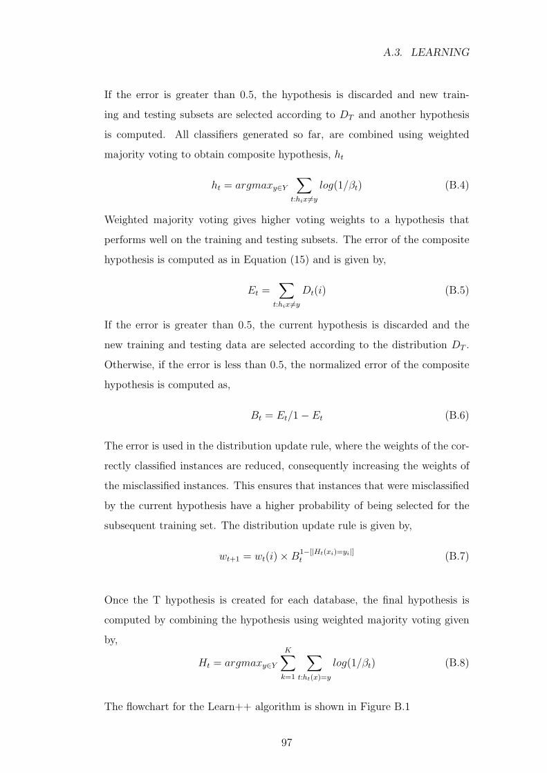
A.3. LEARNING
If the error is greater than 0.5, the hypothesis is discarded and new train-
ing and testing subsets are selected according to DT and another hypothesis
is computed. All classifiers generated so far, are combined using weighted
majority voting to obtain composite hypothesis, ht
ht = argmaxy∈Y
∑t:hix 6=y
log(1/βt) (B.4)
Weighted majority voting gives higher voting weights to a hypothesis that
performs well on the training and testing subsets. The error of the composite
hypothesis is computed as in Equation (15) and is given by,
Et =∑
t:hix 6=y
Dt(i) (B.5)
If the error is greater than 0.5, the current hypothesis is discarded and the
new training and testing data are selected according to the distribution DT .
Otherwise, if the error is less than 0.5, the normalized error of the composite
hypothesis is computed as,
Bt = Et/1− Et (B.6)
The error is used in the distribution update rule, where the weights of the cor-
rectly classified instances are reduced, consequently increasing the weights of
the misclassified instances. This ensures that instances that were misclassified
by the current hypothesis have a higher probability of being selected for the
subsequent training set. The distribution update rule is given by,
wt+1 = wt(i)×B1−[|Ht(xi)=yi|]t (B.7)
Once the T hypothesis is created for each database, the final hypothesis is
computed by combining the hypothesis using weighted majority voting given
by,
Ht = argmaxy∈Y
K∑k=1
∑t:ht(x)=y
log(1/βt) (B.8)
The flowchart for the Learn++ algorithm is shown in Figure B.1
97
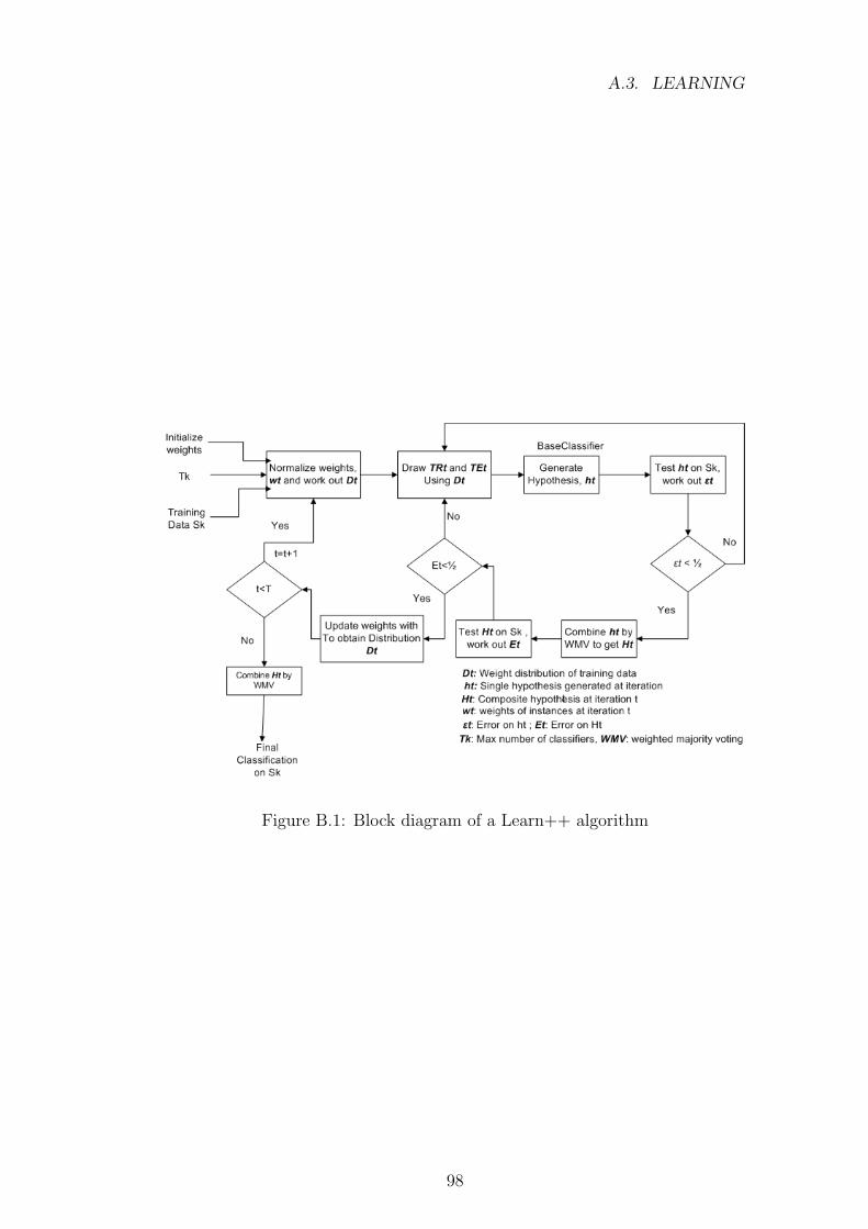
A.3. LEARNING
Figure B.1: Block diagram of a Learn++ algorithm
98
Appendix C
Publications
Below is a list of all publications that have been derived from this work.
• C.B. Vilakazi and T. Marwala, “Bushing Fault Detection and Diagno-
sis using Extension Neural Network”, In Proceeding of the 10th Inter-
national Conference on Intelligent Engineering Systems 2006, London,
England, IEEE, June 2006, pp 170–174.
• C.B. Vilakazi and T. Marwala, “A Multi-agent System for Bushing Con-
dition Monitoring”, In Proceeding of the 17th Symposium of Pattern
Recognition of South Africa, Bloemfontein, South Africa, November
2006, pp. 201–207.
• C.B Vilakazi, T. Marwala, R.P. Mautla and E.M. Moloto, “On-line
Bushing Condition Monitoring”, WSEAS Transactions on Power Sys-
tem, 2006, pp. 380-287.
99
References
[1] C. Bishop, Neural Networks for Pattern Recognition. New York: Oxford
University Press, 2003.
[2] C. Burges, “A tutorial on support vector machines for pattern recognition,”
Data Mining and Knowledge Discovery, vol. 2, pp. 955–974, 1998.
[3] P. Tavner and J. Penman, Condition Monitoring of Electrical Machines.
England: John Wiley & Sons Inc, 1987.
[4] S. McArthur, S. Strachan, and G. Jahn, “The design of a multi-agent sys-
tem for transformer condition monitoring,” IEEE Transactions on Power
System, vol. 19, no. 4, pp. 1845–1852, 2004.
[5] D. N. Chorafas, Knowledge Engineering. Van Nostrand Reinhold, first
edition ed., 1990.
[6] K. Wang, Intelligent Condition Monitoring and Diagnosis System. IOS
Press, 2003.
[7] E. Mangani, S. McArthur, J. R. McDonald, and A. Moyes, “A multi-agent
system for monitoring industrial gas turbine start-up,” IEEE Transactions
on Power System, vol. 16, no. 3, pp. 396–401, 2001.
[8] R. Polikar, L. Udpa, A. S. Udpa, and V. Hanovar, “Learn++: An incremen-
tal learning algorithm for supervised neural networks,” IEEE Transactions
on Systems, Man and Cybernetics, vol. 31, no. 4, pp. 497–508, 2001.
100
REFERENCES
[9] N. Jennings, L. Varga, R. Aarnts, J. Fuchs, and P. Skarek, “Transform-
ing standalone expert systems into a community of cooperating agents,”
Engineering Applications in Artificial Intelligence, pp. 317–331, 1993.
[10] N. R. Jennings, J. Corera, I. Laresgoiti, E. Mamdani, F. Perriolat,
P. Skarek, and L. Z. Varga, “Using ARCHON to develop real-world DAI
applications for electricity transportation management and particle accel-
erator control,” IEEE Expert, pp. 64–70, 1996.
[11] J. H. Williams, A. Davies, and P. R. Drake, Condition–Based Maintenance
and Machine Diagnostics. Chapman and Hall, 1992.
[12] X. Lou and K. Loparo, “Bearing fault diagnosis based on wavelet trans-
form and fuzzy inference,” Mechanical Systems and Signal Processing,
vol. 18, pp. 1077–1095, 2004.
[13] T. Marwala, Fault Identification using Neural Networks and Vibration
Data. PhD thesis, St John College, University of Cambridge, 2001.
[14] B. Samata, “Gear fault detection using artificial neural network and vec-
tor machines with genetic algorithms,” Mechanical Systems and Signal Pro-
cessing, vol. 18, pp. 625 – 644, 2005.
[15] B. Yang, T. Han, and J. An, “ART-KOHONEN neural network for fault
diagnosis of rotating machinery,” Mechanical Systems and Signal Process-
ing, vol. 18, pp. 645 – 657, 2004.
[16] A. Rojas and A. Nandi, “Practical scheme for fast detection and classi-
fication of rolling-element bearing faults using support vector machines,”
Mechanical Systems and Signal Processing, vol. 20, no. 7, pp. 1523–1536,
2006.
[17] B. Samanta and K. R. Al-Bushi, “Artificial neural network based fault
diagnostic of rolling elements bearing using time-domain features,” Me-
chanical Systems and Signal Processing, vol. 17, pp. 317–328, 2003.
101
REFERENCES
[18] B. Yang, T. Han, and W. Hwang, “Fault diagnosis of rotating machin-
ery based on multi-class support vector machines,” Journal of Mechanical
Science and Technology, vol. 19, no. 3, pp. 846 – 859, 2005.
[19] H. M. Ertunc, K. Loparo, and H. Ocak, “Tool wear condition monitoring
in drilling operations using hidden Markov models,” International Journal
of Machine Tools and Manufacture, vol. 41, pp. 1363 – 1384, 2001.
[20] H. Ocak and K. Loparo, “Estimation of the running speed and bearing
defect frequencies of an induction motor from vibration data,” Mechanical
Systems and Signal Processing, vol. 18, pp. 515 – 533, 2004.
[21] V. Purushotham, S. Narayanana, and S. Prasadb, “Multi-fault diagnosis
of rolling bearing elements using wavelet analysis and hidden Markov model
based fault recognition,” NDT and E International, vol. 38, no. 8, pp. 654
– 664, 2005.
[22] Q. Miao and V. Makis, “Condition monitoring and classification of ro-
tating machinery using wavelets and hidden Markov models,” Mechanical
Systems and Signal Processing, vol. 21, no. 2, pp. 840–855, 2007.
[23] T. Marwala, U. Mahola, and F. Nelwamondo, “Hidden Markov models
and Gaussian mixture models for bearing fault detection using fractals,”
in Proceedings of the International Joint Conference on Neural Networks,
pp. 1535 – 1571, 2006.
[24] T. K. Saha, “Review of modern diagnostic techniques for assessing insu-
lation condition in aged transformers,” IEEE Transactions on Electrical
Insulation, vol. 10, no. 5, pp. 903 – 917, 2003.
[25] S. M. Dhlamini and T. Marwala, “Using SVM, RBF and MLP for bush-
ings,” in Proceedings of IEEE Africon, pp. 613 – 617, 2004.
[26] E. Dornenburg and W. Strittmatter, “Monitoring oil-cooled transformers
by gas analysis,” Brown Boveri Rev., vol. 61, no. 5, pp. 238–247, 1974.
102
REFERENCES
[27] R. R. Rogers, “IEEE and IEC codes to interpret faults in transformers us-
ing gas in oil analysis,” IEEE Transactions on Electrical Insulation, vol. 13,
no. 5, pp. 349 – 354, 1978.
[28] M. Duval, “Fault gases formed in oil-filled breathing E.H.V. power trans-
formersthe interpretation of gas analysis data,” in Proceedings of IEEE
Power Engineering Society Conference, pp. C74–476–8, 1974.
[29] IEC Standard 60 599., “Mineral oil-impregnated electrical equipment in
service-guide to the interpretation of dissolved and free gases analysis,”
IEC Std. 60 599., 1969.
[30] S. K. Bhattacharya, R. E. Smith, and T. A. Haskew, “A neural network
approach to transformer fault diagnosis using dissolved gas analysis data,”
in Proceedings of North American Power Symposium, pp. 125 – 129, 1993.
[31] Y. Zhang, X. Ding, Y. Liu, and P. J. Griffin, “An artificial neural net-
work based approach to transformer fault diagnosis,” IEEE Transactions
on Power Delivery, vol. 11, pp. 1836 – 1841, 1996.
[32] Z. Wang, Y. Zhang, C. Li, and Y. Liu, “ANN based transformer fault
diagnosis,” in Proceedings of American Power Conference, pp. 428 – 432,
1997.
[33] Y. M. Tu, J. M. Huang, N. Gao, Z. S. Zhu, and Z. Yan, “Transformer in-
sulation diagnosis based on improved ANN analysis,” in Proceedings of the
IEEE International Conference on Properties and Application of Dielectric
Materials, pp. 263 – 266, 1997.
[34] O. Venegas, Y. Mizuno, K. Naito, and T. Kamiya, “Diagnosis of oil insu-
lated power apparatus by using neural network asimulation,” IEEE Trans-
actions on Power Delivery, vol. 4, pp. 290 – 299, 1997.
[35] D. G. Esp, M. Carrillo, and A. J. McGrail, “Data mining applied to
transformer oil analysis data.,” in Proceedings of the IEEE International
Symposium of Electrical Insulation, pp. 12 – 15, 1998.
103
REFERENCES
[36] Y. C. Huang, H. T. Yang, and C. L. Huang, “Developing a new trans-
former fault diagnosis system through evolutionary fuzzy logic,” IEEE
Transactions on Power Delivery, vol. 12, pp. 761 – 767, 1997.
[37] C. E. Lin, J. M. Ling, and C. L. Huang, “An expert system for transformer
fault diagnosis using dissolved gas analysis,” IEEE Transactions on Power
Delivery, vol. 8, no. 1, pp. 231 – 238, 1993.
[38] K. Tomsovic, M. Tapper, and T. Ingvarsson, “Fuzzy information approach
to integrating different transformer diagnosis methods,” IEEE Transac-
tions on Power Delivery, vol. 8, pp. 1638–1654, 1993.
[39] S. Theodoridis and K. Koutroumbas, Pattern Recognition. New York:
Academic Press, first ed., 1999.
[40] S. Ericsson, N. Grip, E. Johansson, L. Persson, R. Sjoberg, and
J. Stromberg, “Towards automatic detection of local bearing defects in
rotating machines,” Mechanical Systems and Signal Processing, vol. 19,
pp. 509–535, 2004.
[41] J. Wang, J. Wang, and Y. Weng, “Chip design of MFCC extraction for
speech recognition,” The VLSI Journal, vol. 32, pp. 111–131, 2002.
[42] Z. Wang, P. Willet, P. R. DeAguiar, and Y. Webster, “Neural network
detection of grinding burn from acoustic emission,” International Journal
of Machine Tools and Manufacture, vol. 41, pp. 283–309, 2001.
[43] J. Weston and C. Watkins, “Support vector machines for multiclass recog-
nition,” in Proceedings of ESANN99, pp. 219–224, 1999.
[44] V. Vapnik, The Nature of Statistical Learning Theory. Berlin: Springer,
second ed., 1999.
[45] B. Scholkopf, “SVMs a practical consequence of learning theory,” IEEE
Intelligent Systems, vol. 13, pp. 18–19, 1998.
[46] T. K. Wang, “A novel extension method for transformer fault diagnosis,”
IEEE Transactions on Power Delivery, vol. 18, no. 1, pp. 164 – 169, 2003.
104
REFERENCES
[47] G. A. Carpenter, S. Grossberg, N. Markuzon, J. H. Reynolds, and D. B.
Rosen, “Fuzzy ARTMAP: A neural network architecture for incremental
supervised learning of analog multidimensional maps.,” IEEE Transactions
on Neural Networks, vol. 3, pp. 698 – 713, 1992.
[48] M. P. Perrone and L. N. Cooper, Neural Networks for Speech and Image
Processing, ch. When Networks Disagree: Ensemble Methods for Hybrid
Neural Networks. Chapman Hall, 1993.
[49] N. Littlestone and M. Warmuth, “Weighted majority algorithm,” Infor-
mation and Computation, vol. 108, pp. 212–261, 1994.
[50] M. Petrakos, J. A. Benediktsson, and I. Kannellopoulos, “The effect of
classifier agreement on the accuracy of the combined classifier in deci-
sion level fusion,” IEEE Transactions on Geoscience and Remote Sensing,
vol. 39, pp. 2539 – 2546, November 2001.
[51] L. I. Kuncheva, C. J. Whitaker, C. A. Shipp, and R. P. W. Duin, “Limits
of the majority vote accuray in classifier fusion,” Pattern Analysis and
Applications, vol. 6, pp. 22 – 31, 2003.
[52] K. Goebel, W. Z. Yan, and W. Cheetham, “A method to calculate classi-
fiers correlation for decision fusion,” in Proceedings of Decision and Control,
pp. 135 – 140, 2002.
[53] D. Wolpert, “Stacked generalization,” Neural Networks, vol. 5, no. 2,
pp. 241–259, 1992.
[54] J. Kittler, M. Hatef, R. P. W. Duin, and J. Matas, “On combining clas-
sifiers,” IEEE Transactions on Pattern Analysis and Machine Intelligence,
vol. 20, no. 3, pp. 226 – 239, 1998.
[55] S. Rangarajan, P. Jalote, and S. Tripathi, “Capacity of voting systems,”
IEEE Transactions on Software Engineering, vol. 19, no. 7, pp. 698–706,
1993.
105
REFERENCES
[56] C. Ji and S. Ma, “Performance and efficiency: Recent advances in super-
vised learning,” IEEE Proceedings, vol. 87, no. 9, pp. 1519–1535, 1999.
[57] S. K. Chalup, “Incremental learning in biological and machine learning
systems,” International Journal of Neural Systems, vol. 12, no. 6, pp. 90 –
127, 2002.
[58] E. Wang and A. Kuh, “A smart algorithm for incremental learning,”
in Proceedings of International Joint Conference on Neural Networks,
pp. 121–126, 1992.
[59] F. S. Osorio and B. Amy, “INSS: A hybrid system for constructive ma-
chine learning,” Neurocomputing, vol. 28, pp. 191–205, 1999.
[60] M. Vo, “Incremental learning using the time delay neural network,” in
Proceedings of the IEEE International Conference on Acoustics, Speech
and Signal Processing, pp. 629–632, 1994.
[61] T. Hoya and A. G. Constantidines, “A heuristic pattern correction scheme
for grnns and its application to speech recognition,” in Proceedings of the
IEEE Signal Processing Society Workshop, pp. 351–359, 1998.
[62] C. H. Higgins and R. Goodman, “Incremental learning with rule-based
neural networks,” Proceedings of International Joint Conference on Neural
Networks (IJCNN91), vol. 1, pp. 875–880, 1991.
[63] H. Chen and V. Soo, “Design of adaptive and incremental feed-forward
neural networks,” in Proceedings of IEEE International Conference on Neu-
ral Networks (ICNN93), pp. 479–484, 1993.
[64] L. Fu, “Incremental knowledge acquisition in supervised learning net-
works,” IEEE Transactions on Systems, Man, and Cybernatics. Part A:
Systems and Humans, vol. 26, no. 6, pp. 801–809, 1996.
[65] L. Fu, H. H. Hsu, and J. Principe, “Incremental backpropagation learning
networks,” IEEE Transactions on Neural Networks, vol. 7, no. 3, pp. 757–
762, 1996.
106
REFERENCES
[66] P. Mitra, C. Murthy, and S. Pal, “Data condensation in large databases
by incremental learning with support vector machines,” Proceedings of 15th
International Conference on Pattern Recognition, vol. 2, pp. 708– 711,
2000.
[67] K. Li and H. Huang, “Incremental learning proximal support vector
machine classifiers,” Proceedings of International Conference on Machine
Learning and Cybernetics, vol. 3, pp. 1635–1637, 2002.
[68] K. Loparo, “Bearing vibration data set,
Case Western Reserve University.” Internet Listing, Last Acessed: Febru-
ary 2006. URL: http://www.eecs.cwru.edu/laboratory/bearing/
download.htm.
[69] R. Polikar, Algorithms for enhancing pattern separability, feature selection
and incremental learning with applications to gas sensing electronic nose
systems. PhD thesis, Department of Electrical Engineering, Iowa State
University, 2001.
[70] M. Wooldridge, An Introduction to Multiagent System. England: John
Wiley and Sons, 2001.
[71] J. Lind, “Iterative software engineering for multiagent systems
The MASSIVE Method,” Lecture Notes in Artificial Intelligence, Springer-
Verlag, Berlin, 2001.
[72] S. Parka and V. Sugumaran, “Designing multi-agent systems: A frame-
work and application,” Expert Systems with Applications, vol. 28, pp. 259–
271, 2005.
[73] M. Markey, G. Tourassi, M. Margolis, and D. DeLong, “Impact of missing
data in evaluating artificial neural networks trained on complete data,”
Computers in Biology and Medicine, vol. 36, pp. 516–525, 2006.
107

REFERENCES
[74] “Fipa specifications Foundation for Intelligent Physical
Agents.” Internet Listing, Last Acessed: July 2006. URL:
http://www.fipa.org/specifications/index.html.
[75] C. Lim and R. F. Harrison, “An incremental adaptive network for on-line
supervised learning and propability estimation,” Neural Networks, vol. 10,
no. 5, pp. 925 – 939, 1997.
108