Embed Size (px)
Citation preview
2361-17
School on Large Scale Problems in Machine Learning and Workshop on Common Concepts in Machine Learning and Statistical Physics
Ole WINTHER
20 - 31 August 2012
Technical University of Denmark DTU and University of Copenhagen KU Denmark
MACHINE LEARNING IN SYSTEMS BIOLOGY: Factor Modeling 'Identifiability and Sparsity - Learning Models of Genomic Data'
Introduction PCA ICA Factor modeling Physics SLIM Summary
Factor ModelingIdentifiability and Sparsity - Learning models of genomic
data
Ole Winther
Technical University of Denmark (DTU)
August 21, 2012
Ole Winther DTU
Introduction PCA ICA Factor modeling Physics SLIM Summary
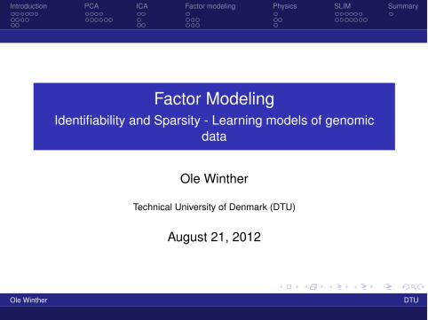
Motivation – multivariate data
Google vision: develop the “perfect search engine,” defined byco-founder Larry Page as something that, “understands exactlywhat you mean and gives you back exactly what you want.”
Ole Winther DTU
Introduction PCA ICA Factor modeling Physics SLIM Summary
Motivation – multivariate data
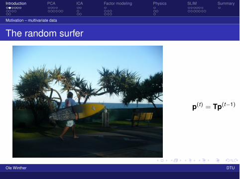
The random surfer
p(t) = Tp(t−1)
Ole Winther DTU
Introduction PCA ICA Factor modeling Physics SLIM Summary
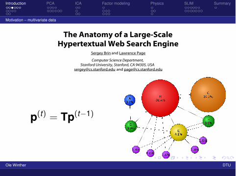
Motivation – multivariate data
The Anatomy of a Large-Scale Hypertextual Web Search Engine
Sergey Brin and Lawrence Page
Computer Science Department,Stanford University, Stanford, CA 94305, USA
[email protected] and [email protected]
Abstract In this paper, we present Google, a prototype of a large-scale search engine which makes heavy use of the structure present in hypertext. Google is designed to crawl and index the Web efficiently and produce much more satisfying search results than existing systems. The prototype with a full text and hyperlink database of at least 24 million pages is available at http://google.stanford.edu/ To engineer a search engine is a challenging task. Search engines index tens to hundreds of millions of web pages involving a comparable number of distinct terms. They answer tens of millions of queries every day. Despite the importance of large-scale search engines on the web, very little academic research has been done on them. Furthermore, due to rapid advance in technology and web proliferation, creating a web search engine today is very different from three years ago. This paper provides an in-depth description of our large-scale web search engine -- the first such detailed public description we know of to date. Apart from the problems of scaling traditional search techniques to data of this magnitude, there are new technical challenges involved with using the additional information present in hypertext to produce better search results. This paper addresses this question of how to build a practical large-scale system which can exploit the additional information present in hypertext. Also we look at the problem of how to effectively deal with uncontrolled hypertext collections where anyone can publish anything they want.
Keywords World Wide Web, Search Engines, Information Retrieval, PageRank, Google
1. Introduction
(Note: There are two versions of this paper -- a longer full version and a shorter printed version. The full version is available on the web and the conference CD-ROM.) The web creates new challenges for information retrieval. The amount of information on the web is growing rapidly, as well as the number of new users inexperienced in the art of web research. People are likely to surf the web using its link graph, often starting with high quality human maintained indices such as http://www7.scu.edu.au/programme/fullpapers/1921/com1921.htm 1
p(t) = Tp(t−1)
Ole Winther DTU
Introduction PCA ICA Factor modeling Physics SLIM Summary
Motivation – multivariate data
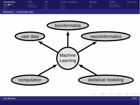
MachineLearning
neuroinformatics
bioinformatics
user data
computation statistical modeling
Ole Winther DTU
Introduction PCA ICA Factor modeling Physics SLIM Summary
Motivation – multivariate data
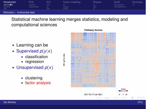
Statistical machine learning merges statistics, modeling andcomputational sciences
• Learning can be• Supervised p(y |x)
• classification• regression
• Unsupervised p(x)
• clustering• factor analysis
Ole Winther DTU

Introduction PCA ICA Factor modeling Physics SLIM Summary
Motivation – multivariate data
• Data is often (but not always) represented as a matrix of dfeatures and N samples:
size(X) = [d N]
• In stats d = p, N = n and data matrix transposed X → XT
• Collaborative filtering:
X = item-user matrix
• Gene expression:
X = gene-tissue matrix
• Text analysis:
X = term-document matrix
• Neuro-informatics: X = sensor-time seriesOle Winther DTU

Introduction PCA ICA Factor modeling Physics SLIM Summary
Continuous latent variable models
• vn : “taste” vector of viewer n, length(vn) = K .• um : “profile” vector movie m.• Rating model:
rmn = um · vn + �mn
• Learn U and V from rating matrix. Computation!Ole Winther DTU
Introduction PCA ICA Factor modeling Physics SLIM Summary
Continuous latent variable models
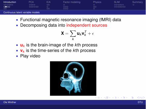
• Functional magnetic resonance imaging (fMRI) data• Decomposing data into independent sources
X =�
k
ukvTk + �
• uk is the brain-image of the k th process• vk is the time-series of the k th process• Play video
Ole Winther DTU
Introduction PCA ICA Factor modeling Physics SLIM Summary
Continuous latent variable models
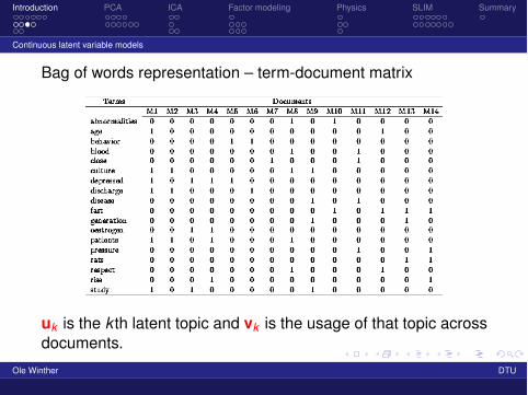
Bag of words representation – term-document matrix
uk is the k th latent topic and vk is the usage of that topic acrossdocuments.
Ole Winther DTU

Introduction PCA ICA Factor modeling Physics SLIM Summary
Continuous latent variable models
• Gene expression profiling – simultaneous measurement of50k genes (mRNA levels).
• Use library of gene sets representing response to geneticand chemical perturbations.
• Covariation (redundancy) – use factor model
X = WZ + E
200 patient samples
Ole Winther DTU
Introduction PCA ICA Factor modeling Physics SLIM Summary
Overview
Roadmap / (learning objectives)
• Principal component analysis (PCA)• Independent component analysis (ICA) - identifiability• Factor modeling - Bayesian formulation with sparsity• Insights from physics - fundamental limitations for learning
covariance structure• Sparse linear identifiable modeling (SLIM) - learning
models of genomic data• + exercises and breaks!
Ole Winther DTU

Introduction PCA ICA Factor modeling Physics SLIM Summary
Overview
• Reading material:• PCA: Bishop (Pattern Recogniyion and Machine Learning)
12-12.2.1, 12.1.2 and 12.2.1• ICA: Bishop 12.4-12.4.1• Factor analysis: 12.2.4 and in case story below• Covariance learning: Hoyle and Rattray, 2003+2004;
Alexei Onatski, 2007• Henao and Winther, 2011; Shimizu et. al., 2006; Carvalho
et. al., 2008. http://cogsys.imm.dtu.dk/slim
Ole Winther DTU
Introduction PCA ICA Factor modeling Physics SLIM Summary
Principal Component Analysis (PCA)
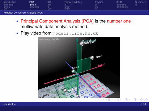
• Principal Component Analysis (PCA) is the number onemultivariate data analysis method.
• Play video from models.life.ku.dk
Ole Winther DTU
Introduction PCA ICA Factor modeling Physics SLIM Summary
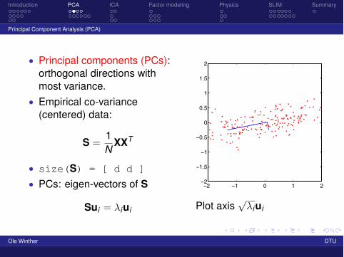
Principal Component Analysis (PCA)
• Principal components (PCs):orthogonal directions withmost variance.
• Empirical co-variance(centered) data:
S =1N
XXT
• size(S) = [ d d ]
• PCs: eigen-vectors of S
Sui = λiui
−2 −1 0 1 2−2
−1.5
−1
−0.5
0
0.5
1
1.5
2
Plot axis√λiui
Ole Winther DTU
Introduction PCA ICA Factor modeling Physics SLIM Summary
Principal Component Analysis (PCA)
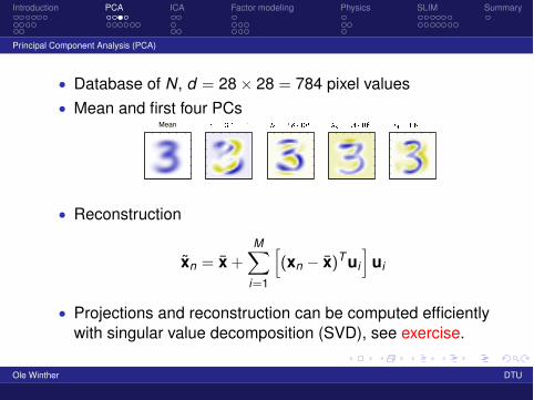
• Database of N, d = 28 × 28 = 784 pixel values• Mean and first four PCs
Mean
• Reconstruction
x̃n = x̄ +M�
i=1
�(xn − x̄)T ui
�ui
• Projections and reconstruction can be computed efficientlywith singular value decomposition (SVD), see exercise.
Ole Winther DTU
Introduction PCA ICA Factor modeling Physics SLIM Summary
Principal Component Analysis (PCA)
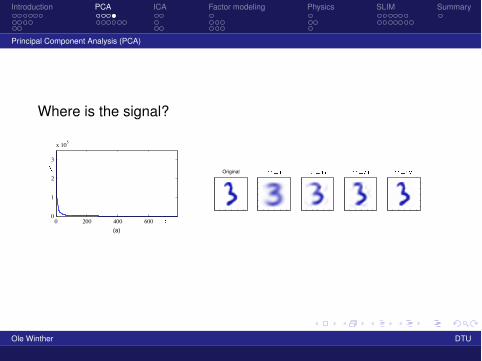
Where is the signal?
(a)0 200 400 600
0
1
2
3
x 105
Original
Ole Winther DTU
Introduction PCA ICA Factor modeling Physics SLIM Summary
Probabilistic PCA
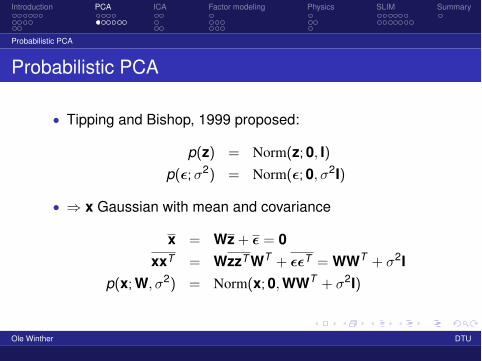
Probabilistic PCA
• Tipping and Bishop, 1999 proposed:
p(z) = Norm(z; 0, I)p(�;σ2) = Norm(�; 0,σ2I)
• ⇒ x Gaussian with mean and covariance
x = Wz + � = 0xxT = WzzT WT + ��T = WWT + σ2I
p(x;W,σ2) = Norm(x; 0,WWT + σ2I)
Ole Winther DTU

Introduction PCA ICA Factor modeling Physics SLIM Summary
Probabilistic PCA
• Log likelihood for W and σ2 is joint distribution of all data:
log L(θ;X) =�
nlog p(xn|W,σ2)
= −N2
�log det 2πΣ+ Tr
�Σ−1S
��
• Model covariance: Σ = WWT + σ2I• Empirical covariance: S = 1
N XXT
• Maximum likelihood: WML is spanned by first M PCs• The remaining variance is fitted by σ2I,
σ2ML =
d�
i=M+1
λi/(d − M) .
• Example of structured covariance estimation.Ole Winther DTU
Introduction PCA ICA Factor modeling Physics SLIM Summary
Probabilistic PCA
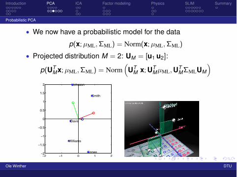
• We now have a probabilistic model for the data
p(x;µML,ΣML) = Norm(x;µML,ΣML)
• Projected distribution M = 2: UM = [u1 u2]:
p(UTMx;µML,ΣML) = Norm
�UT
M x;UTMµML,UT
MΣMLUM
�
2 1 0 1 22
1.5
1
0.5
0
0.5
1
1.5
2
Smith
Johnson
Williams
Jones
Davis
Ole Winther DTU

Introduction PCA ICA Factor modeling Physics SLIM Summary
Probabilistic PCA
• We now have a probabilistic model for the data
p(x;µML,ΣML) = N (x;µML,ΣML)
• Projected distribution M = 2: UM = [u1u2]:
p(UTMx;µML,ΣML) = N
�UT
M x;UTMµML,UT
MΣMLUM
�
2 1 0 1 22
1.5
1
0.5
0
0.5
1
1.5
2
Smith
Johnson
Williams
Jones
Davis
Ole Winther DTU
Introduction PCA ICA Factor modeling Physics SLIM Summary
Probabilistic PCA
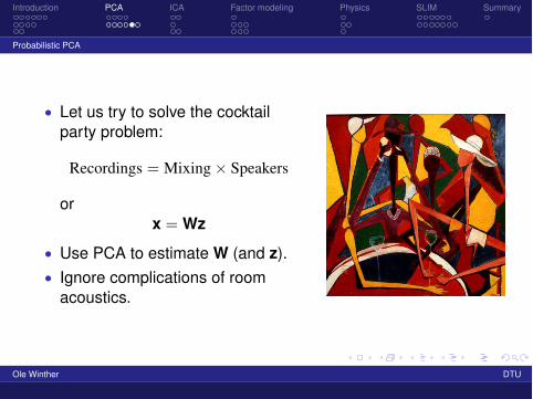
• Let us try to solve the cocktailparty problem:
Recordings = Mixing × Speakers
orx = Wz
• Use PCA to estimate W (and z).• Ignore complications of room
acoustics.
Ole Winther DTU
Introduction PCA ICA Factor modeling Physics SLIM Summary
Probabilistic PCA
• Stop sign! Non-uniqueness of solution!• Likelihood only depends upon W through Σ = WWT + σ2I• Rotate W:
W ← �WU
• leave covariance unchanged
WWT = �WUUT �W = �W �WT .
Ole Winther DTU
Introduction PCA ICA Factor modeling Physics SLIM Summary
Independent component analysis (ICA)
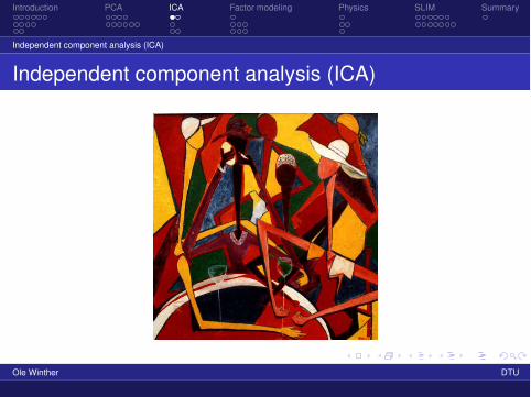
Independent component analysis (ICA)
Ole Winther DTU
Introduction PCA ICA Factor modeling Physics SLIM Summary
Independent component analysis (ICA)
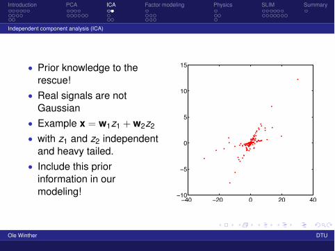
• Prior knowledge to therescue!
• Real signals are notGaussian
• Example x = w1z1 + w2z2
• with z1 and z2 independentand heavy tailed.
• Include this priorinformation in ourmodeling!
−40 −20 0 20 40−10
−5
0
5
10
15
Ole Winther DTU
Introduction PCA ICA Factor modeling Physics SLIM Summary
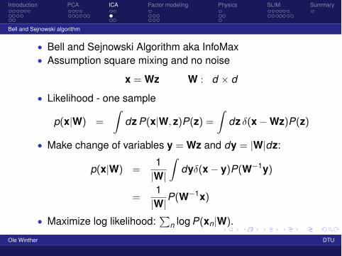
Bell and Sejnowski algorithm
• Bell and Sejnowski Algorithm aka InfoMax• Assumption square mixing and no noise
x = Wz W : d × d
• Likelihood - one sample
p(x|W) =
�dz P(x|W, z)P(z) =
�dz δ(x − Wz)P(z)
• Make change of variables y = Wz and dy = |W|dz:
p(x|W) =1|W|
�dyδ(x − y)P(W−1y)
=1|W|P(W−1x)
• Maximize log likelihood:�
n log P(xn|W).
Ole Winther DTU

Introduction PCA ICA Factor modeling Physics SLIM Summary
Identifiability
• If a statistical model p(x; θ) has the property that
p(x; θ) = p(x; θ�) ⇒ θ = θ� for all θ, θ� ∈ Θ.
• then the model is said to be identifiability.• The pPCA model is not identifiable since W and WU give
same model.• Many variants of ICA can be proven to be identifiable,
Kagan et. al., 1973 and Comon, 1994.• up to arbitrary permutation P and sign Sign:
z → Sign P z W → −W P−1 Sign
• PCA not strictly a statistical model, but PC projectionsidentifiable up to sign.
Ole Winther DTU
Introduction PCA ICA Factor modeling Physics SLIM Summary
Identifiability
• Matlab exercises on these topics available fromhttp://www.imm.dtu.dk/Forskning/ISP/
Undervisning/02901_2012.aspx
• (For offline use)• Student Exercise 1
• PCA and ICA on cocktail party problem - identifiability• Student Exercise 2
• Singular value decomposition (SVD) for PCA
Ole Winther DTU
Introduction PCA ICA Factor modeling Physics SLIM Summary
Factor modeling
Factor modeling
• A bit of history• Invented by Spearman 1904. A single underlying g-factor
can explain most of variation in cognitive tests.• Raymond Cattell expanded on Spearman’s idea of a
two-factor theory of intelligence and developed 16Personality Factors.
• Widely used in any field working with multivariate data:Psychology, Economy, Bioinformatics,...
• Vanilla Bayes - Gaussian factors and Gaussian weights.• Non-identifiable and identifiable models• Sparsity and model selection
Ole Winther DTU
Introduction PCA ICA Factor modeling Physics SLIM Summary
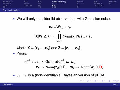
Bayesian formulation
• We will only consider iid observations with Gaussian noise:
xn =Wzn + �n
X|W,Z,Ψ ∼N�
n=1
Norm(xn|Wzn,Ψ) ,
where X = [x1 . . . xN ] and Z = [z1 . . . zN ].• Priors:
ψ−1i |ss, sr ∼ Gamma(ψ−1
i , ss, sr )
zn ∼ Norm(zn|0, I) , wj ∼ Norm(wj |0,D)
• ψi = ψ is a (non-identifiable) Bayesian version of pPCA.
Ole Winther DTU
Introduction PCA ICA Factor modeling Physics SLIM Summary
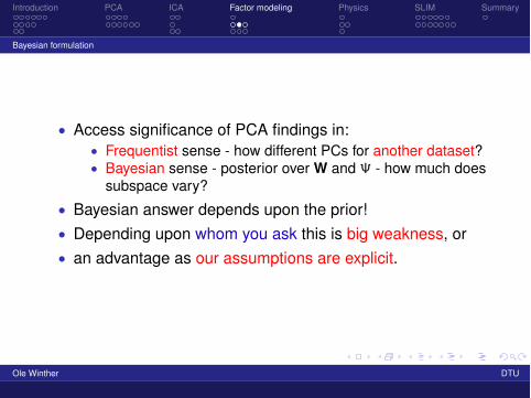
Bayesian formulation
• Access significance of PCA findings in:• Frequentist sense - how different PCs for another dataset?• Bayesian sense - posterior over W and Ψ - how much does
subspace vary?• Bayesian answer depends upon the prior!• Depending upon whom you ask this is big weakness, or• an advantage as our assumptions are explicit.
Ole Winther DTU
Introduction PCA ICA Factor modeling Physics SLIM Summary
Bayesian formulation
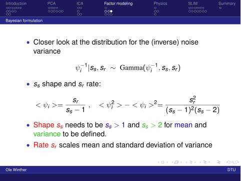
• Closer look at the distribution for the (inverse) noisevariance
ψ−1i |ss, sr ∼ Gamma(ψ−1
i , ss, sr )
• ss shape and sr rate:
< ψi >=sr
ss − 1, < ψ2
i > − < ψi >2=
s2r
(ss − 1)2(ss − 2)
• Shape ss needs to be ss > 1 and ss > 2 for mean andvariance to be defined.
• Rate sr scales mean and standard deviation of variance
Ole Winther DTU

Introduction PCA ICA Factor modeling Physics SLIM Summary
Posterior inference - an example
• MCMC: draw samples, W(r),Ψ(r) from posterior p(W,Ψ|X)• Plot contours of covariance samples and expected value
�Σ�W|X ≈ 1R
R�
r
�W(r)(W(r))T +Ψ(r)
�
• Prior ss = 2 and sr = 1: var(ψi) =s2
r(ss−1)2(ss−2) = ∞.
2 1 0 1 22
1.5
1
0.5
0
0.5
1
1.5
2
Smith
Johnson
Williams
Jones
Davis
2 1 0 1 22
1.5
1
0.5
0
0.5
1
1.5
2
Smith
Johnson
Williams
Jones
Davis
Ole Winther DTU
Introduction PCA ICA Factor modeling Physics SLIM Summary
Posterior inference - an example
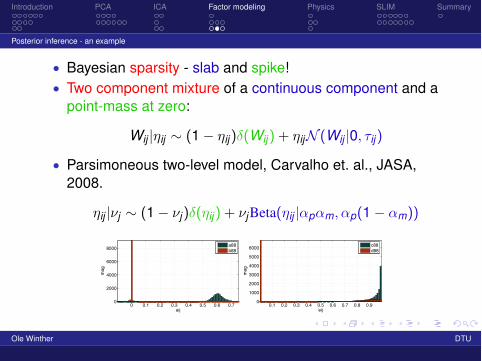
• Bayesian sparsity - slab and spike!• Two component mixture of a continuous component and a
point-mass at zero:
Wij |ηij ∼ (1 − ηij)δ(Wij) + ηijN (Wij |0, τij)
• Parsimoneous two-level model, Carvalho et. al., JASA,2008.
ηij |νj ∼ (1 − νj)δ(ηij) + νjBeta(ηij |αpαm,αp(1 − αm))
0 0.1 0.2 0.3 0.4 0.5 0.6 0.70
2000
4000
6000
8000
aij
mag
a88b88
0.1 0.2 0.3 0.4 0.5 0.6 0.7 0.8 0.90
1000
2000
3000
4000
5000
6000
eij
mag
c88d88
Ole Winther DTU
Introduction PCA ICA Factor modeling Physics SLIM Summary
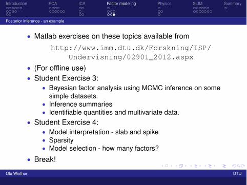
Posterior inference - an example
• Matlab exercises on these topics available fromhttp://www.imm.dtu.dk/Forskning/ISP/
Undervisning/02901_2012.aspx
• (For offline use)• Student Exercise 3:
• Bayesian factor analysis using MCMC inference on somesimple datasets.
• Inference summaries• Identifiable quantities and multivariate data.
• Student Exercise 4:• Model interpretation - slab and spike• Sparsity• Model selection - how many factors?
• Break!
Ole Winther DTU
Introduction PCA ICA Factor modeling Physics SLIM Summary
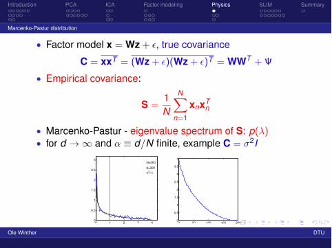
Marcenko-Pastur distribution
• Factor model x = Wz + �, true covariance
C = xxT = (Wz + �)(Wz + �)T = WWT +Ψ
• Empirical covariance:
S =1N
N�
n=1
xnxTn
• Marcenko-Pastur - eigenvalue spectrum of S: p(λ)• for d → ∞ and α ≡ d/N finite, example C = σ2I
0 1 2 3 40
0.5
1
1.5
2
2.5
3N=200
d=2002=1
0 50 100 150 2000
0.5
1
1.5
2
2.5
3
3.5
4
Ole Winther DTU
Introduction PCA ICA Factor modeling Physics SLIM Summary
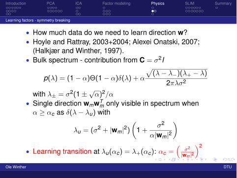
Learning factors - symmetry breaking
• How much data do we need to learn direction w?• Hoyle and Rattray, 2003+2004; Alexei Onatski, 2007;
(Halkjær and Winther, 1997).• Bulk spectrum - contribution from C = σ2I
p(λ) = (1 − α)Θ(1 − α)δ(λ) + α
�(λ− λ−)(λ+ − λ)
2πλσ2
with λ± = σ2(1 ±√α)2/α
• Single direction wmwTm only visible in spectrum when
α ≥ αc as δ(λ− λu) with
λu = (σ2 + |wm|2)�
1 +σ2
α|wm|2
�
• Learning transition at λu(αc) = λ+(αc): αc =�
σ2
|wm|2
�2
Ole Winther DTU
Introduction PCA ICA Factor modeling Physics SLIM Summary
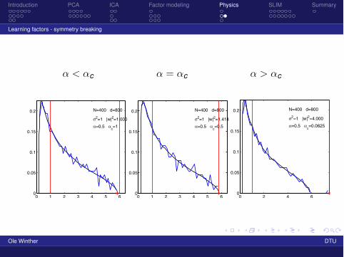
Learning factors - symmetry breaking
α < αc α = αc α > αc
0 1 2 3 4 5 60
0.05
0.1
0.15
0.2 N=400 d=800
2=1 |w|2=1.000
=0.5 c=1
0 1 2 3 4 5 60
0.05
0.1
0.15
0.2 N=400 d=800
2=1 |w|2=1.414
=0.5 c=0.5
0 2 4 60
0.05
0.1
0.15
0.2 N=400 d=800
2=1 |w|2=4.000
=0.5 c=0.0625
Ole Winther DTU

Introduction PCA ICA Factor modeling Physics SLIM Summary
Infinite factor model w Indian Buffet Process
• The number of factors should adapt to data.• Knowles and Ghahramani, 2004+2011 model the sparsity
pattern in W with an Indian Buffet Process.• Model has an infinite number of factors but only a finite
number is active.• Number of active factors adapt approximately to the
number of orthogonal directions with
|w2m| ≥
dNσ2
Ole Winther DTU
Introduction PCA ICA Factor modeling Physics SLIM Summary
Sparse linear identifiable modeling (SLIM)
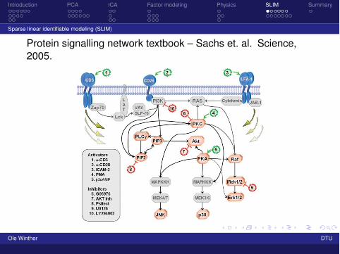
Protein signalling network textbook – Sachs et. al. Science,2005.
Ole Winther DTU
Introduction PCA ICA Factor modeling Physics SLIM Summary
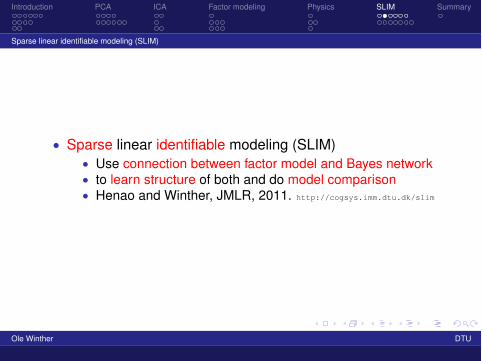
Sparse linear identifiable modeling (SLIM)
• Sparse linear identifiable modeling (SLIM)• Use connection between factor model and Bayes network• to learn structure of both and do model comparison• Henao and Winther, JMLR, 2011. http://cogsys.imm.dtu.dk/slim
Ole Winther DTU
Introduction PCA ICA Factor modeling Physics SLIM Summary
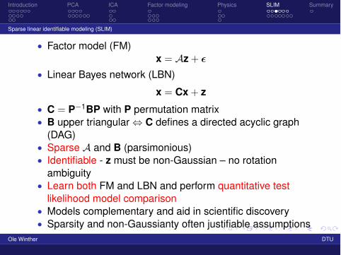
Sparse linear identifiable modeling (SLIM)
• Factor model (FM)x = Az + �
• Linear Bayes network (LBN)
x = Cx + z
• C = P−1BP with P permutation matrix• B upper triangular ⇔ C defines a directed acyclic graph
(DAG)• Sparse A and B (parsimonious)• Identifiable - z must be non-Gaussian – no rotation
ambiguity• Learn both FM and LBN and perform quantitative test
likelihood model comparison• Models complementary and aid in scientific discovery• Sparsity and non-Gaussianty often justifiable assumptions
Ole Winther DTU
Introduction PCA ICA Factor modeling Physics SLIM Summary
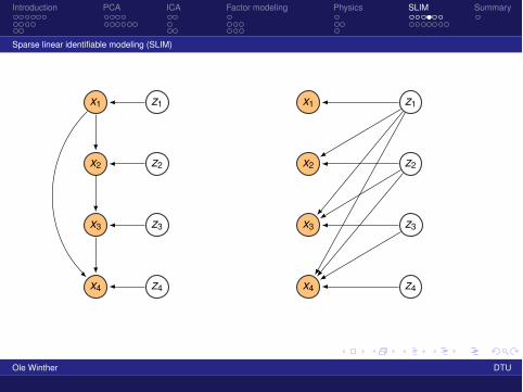
Sparse linear identifiable modeling (SLIM)
x1 z1
x2 z2
x3 z3
x4 z4
x1
x2
x3
x4
z1
z2
z3
z4
Ole Winther DTU
Introduction PCA ICA Factor modeling Physics SLIM Summary
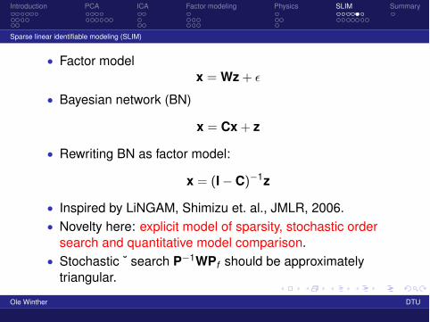
Sparse linear identifiable modeling (SLIM)
• Factor modelx = Wz + �
• Bayesian network (BN)
x = Cx + z
• Rewriting BN as factor model:
x = (I − C)−1z
• Inspired by LiNGAM, Shimizu et. al., JMLR, 2006.• Novelty here: explicit model of sparsity, stochastic order
search and quantitative model comparison.• Stochastic ˘ search P−1WPf should be approximately
triangular.
Ole Winther DTU
Introduction PCA ICA Factor modeling Physics SLIM Summary
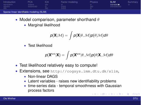
Sparse linear identifiable modeling (SLIM)
• Model comparison, parameter shorthand θ• Marginal likelihood
p(X|M) =
�p(X|θ,M)p(θ|M)dθ
• Test likelihood
p(Xtest|X) =�
p(Xtest|θ,M)p(θ|X,M)dθ
• Test likelihood relatively easy to compute!• Extensions, see http://cogsys.imm.dtu.dk/slim,
• Non-linear DAGS• Latent variables - raises new identifiability problems• time-series data - temporal smoothness with Gaussian
process factors
Ole Winther DTU
Introduction PCA ICA Factor modeling Physics SLIM Summary
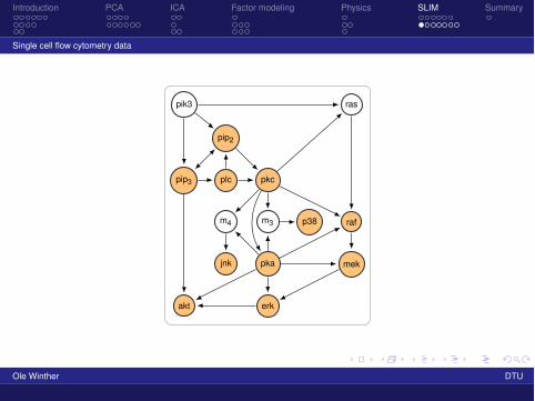
Single cell flow cytometry data
pkc
m3m4
pka
p38
jnk
raf
mek
erk
plc
pip2
pip3
pik3
akt
ras
Ole Winther DTU
Introduction PCA ICA Factor modeling Physics SLIM Summary
Single cell flow cytometry data
• Single cell flow cytometry measurements of 11phosphorylated proteins and phospholipids.
• Data was generated from a series of stimulatory cues andinhibitory interventions.
• Observational data: 1755 general stimulatory conditions,• Experimental data ∼ 80% not used in our approach.• Not “small n large p”!
Ole Winther DTU
Introduction PCA ICA Factor modeling Physics SLIM Summary
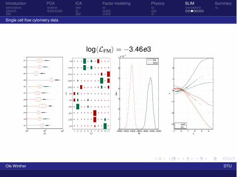
Single cell flow cytometry data
log�LFM� = −3.46e3
100
102
104
raf
mek
plcy
pip2
pip3
erk
akt
pka
pkc
p38
jnk
xx fac
var
1 2 3 4 5 6 7 8 9 10 11
raf
mek
plcy
pip2
pip3
erk
akt
pka
pkc
p38
jnk
4400 4200 4000 3800 3600 3400 32000
1
2
3
4
5
6
7x 10
3
lik
den
FMDAG
−1 0 1 2 3 4
−3
−2
−1
0
1
2
x
y
pip3_plc_
Ole Winther DTU

Introduction PCA ICA Factor modeling Physics SLIM Summary
Single cell flow cytometry data
log�LDAG� = −4.30e3
pkc
pka
p38jnk raf
mek
erk
plc
pip2
pip3
akt
Ole Winther DTU

Introduction PCA ICA Factor modeling Physics SLIM Summary
Single cell flow cytometry data
log�LDAG� = −4.10e3
pkc
pka
p38jnk raf
mek
erk
plc
pip2
pip3
akt
Ole Winther DTU
Introduction PCA ICA Factor modeling Physics SLIM Summary
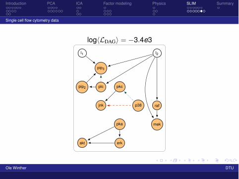
Single cell flow cytometry data
log�LDAG� = −3.4e3
pkc
pka
p38jnk raf
mek
erk
plc
pip3
pip2
akt
l1 l2
Ole Winther DTU
Introduction PCA ICA Factor modeling Physics SLIM Summary
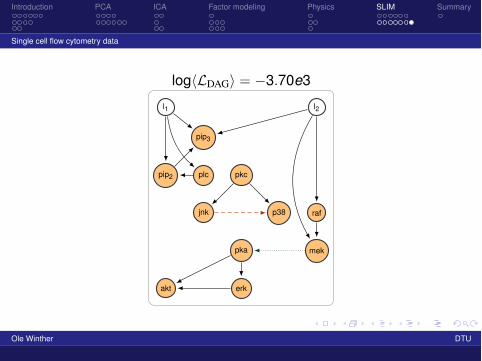
Single cell flow cytometry data
log�LDAG� = −3.70e3
pkc
pka
p38jnk raf
mek
erk
plc
pip3
pip2
akt
l1 l2
Ole Winther DTU

Introduction PCA ICA Factor modeling Physics SLIM Summary
Summary
• Factor models - from PCA to• identifiable models (ICA) and• sparsity (model selection)
• We can learn learn model structurewhen N � d
• Markov chain Monte Carlo - used asstandard inference tool.
• Thank you!
Ole Winther DTU