Final Exam Section 2 May 11th

7:30 am-10:00 am HH 076

Managerial Economics & Business Strategy

Grading Scale

• 5% - Attendance • 8% - Homework (Drop the lowest grade) • 7% - Quizzes (Drop the lowest grade) • 20% - Test 1 • 20% - Test 2 • 20% - Final exam • 5 % - Discussion and participation • 5% - Presentation • 10%- Project report

Overview

• Cumulative • 20 Multiple Choice Questions (40 points) • 4 Essay Questions (60 points) • 1 Bonus Question (4 points)

• Review questions, Final exam sheet, Lecture notes,

(problems solved in class) and Quizzes

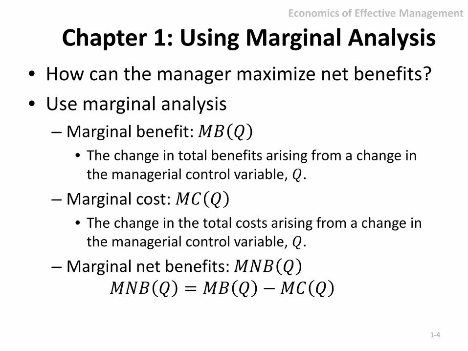
• How can the manager maximize net benefits? • Use marginal analysis

– Marginal benefit: 𝑀𝑀𝑀𝑀 𝑄𝑄 • The change in total benefits arising from a change in

the managerial control variable, 𝑄𝑄.

– Marginal cost: 𝑀𝑀𝐶𝐶 𝑄𝑄 • The change in the total costs arising from a change in

the managerial control variable, 𝑄𝑄.

– Marginal net benefits: 𝑀𝑀𝑀𝑀𝑀𝑀 𝑄𝑄 𝑀𝑀𝑀𝑀𝑀𝑀 𝑄𝑄 = 𝑀𝑀𝑀𝑀 𝑄𝑄 −𝑀𝑀𝐶𝐶 𝑄𝑄

1-4

Economics of Effective Management

Chapter 1: Using Marginal Analysis

• Marginal principle – To maximize net benefits, the manager should

increase the managerial control variable up to the point where marginal benefits equal marginal costs. This level of the managerial control variable corresponds to the level at which marginal net benefits are zero; nothing more can be gained by further changes in that variable.

1-5

Economics of Effective Management

Chapter 1: Marginal Analysis Principle

Chapter 2: Demand Shifters • Income

– Normal good – Inferior good

• Prices of related goods – Substitute goods – Complement goods

• Advertising and consumer tastes • Population • Consumer expectations • Other factors

2-6

Demand

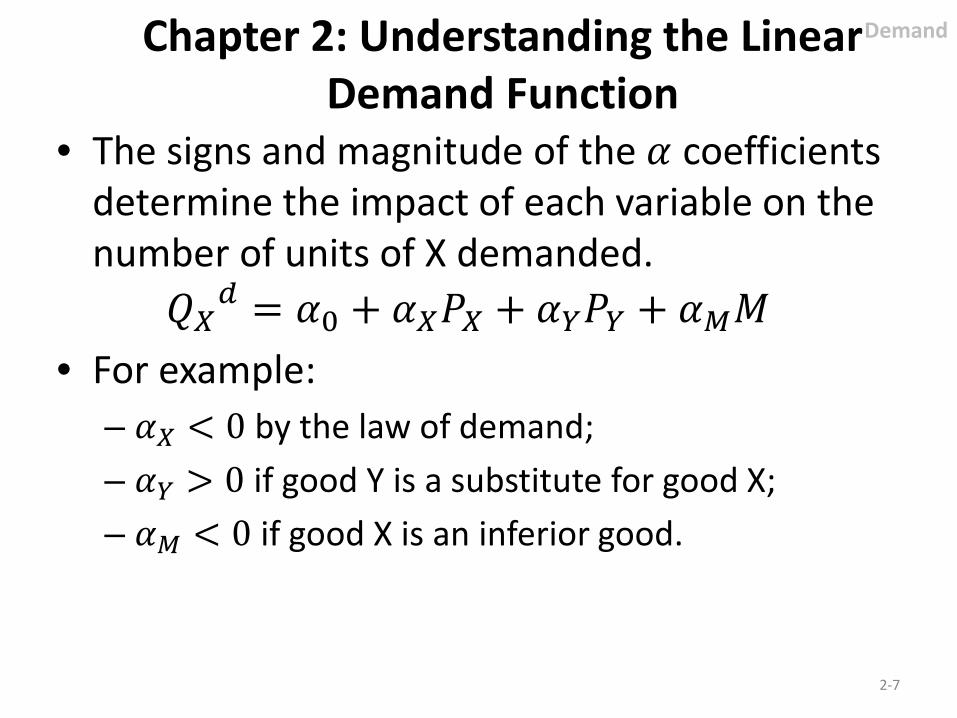
• The signs and magnitude of the 𝛼𝛼 coefficients determine the impact of each variable on the number of units of X demanded.

𝑄𝑄𝑋𝑋𝑑𝑑 = 𝛼𝛼0 + 𝛼𝛼𝑋𝑋𝑃𝑃𝑋𝑋 + 𝛼𝛼𝑌𝑌𝑃𝑃𝑌𝑌 + 𝛼𝛼𝑀𝑀𝑀𝑀 • For example:

– 𝛼𝛼𝑋𝑋 < 0 by the law of demand; – 𝛼𝛼𝑌𝑌 > 0 if good Y is a substitute for good X; – 𝛼𝛼𝑀𝑀 < 0 if good X is an inferior good.

2-7

Demand Chapter 2: Understanding the Linear Demand Function

Quantity in liters

Price per liter

Demand

$5

0

$3

$2

1 2

$1

4 5

2-8

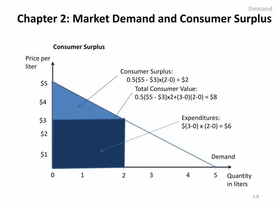
Total Consumer Value: 0.5($5 - $3)x2+(3-0)(2-0) = $8

Expenditures: $(3-0) x (2-0) = $6

Consumer Surplus: 0.5($5 - $3)x(2-0) = $2

Demand

Chapter 2: Market Demand and Consumer Surplus

$4

3

Consumer Surplus

• Input prices • Technology or government regulation • Number of firms

– Entry – Exit

• Substitutes in production • Taxes

– Excise tax – Ad valorem tax

• Producer expectations

2-9

Supply

Chapter 2: Supply Shifters

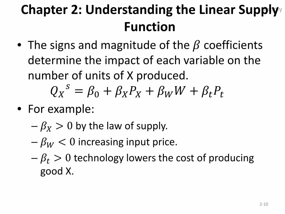
• The signs and magnitude of the 𝛽𝛽 coefficients determine the impact of each variable on the number of units of X produced.

𝑄𝑄𝑋𝑋𝑠𝑠 = 𝛽𝛽0 + 𝛽𝛽𝑋𝑋𝑃𝑃𝑋𝑋 + 𝛽𝛽𝑊𝑊𝑊𝑊 + 𝛽𝛽𝑡𝑡𝑃𝑃𝑡𝑡 • For example:

– 𝛽𝛽𝑋𝑋 > 0 by the law of supply. – 𝛽𝛽𝑊𝑊 < 0 increasing input price. – 𝛽𝛽𝑡𝑡 > 0 technology lowers the cost of producing

good X.

2-10

Supply Chapter 2: Understanding the Linear Supply Function

2-11

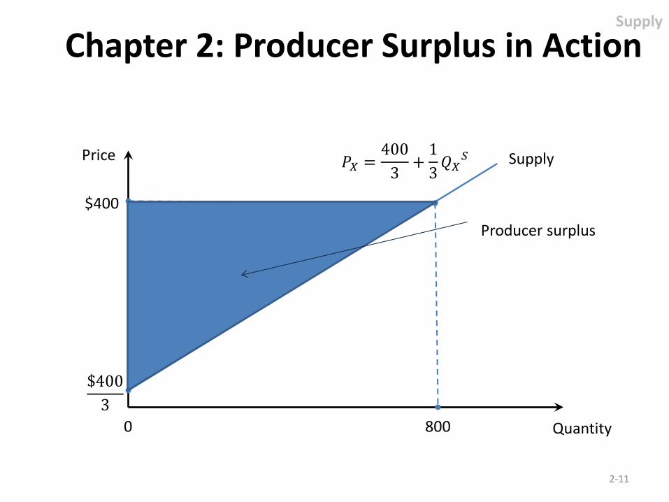
Chapter 2: Producer Surplus in Action

Quantity

Price Supply

$400

0 800

𝑃𝑃𝑋𝑋 =400

3 +13𝑄𝑄𝑋𝑋

𝑆𝑆

Supply

$4003

Producer surplus

• Comparative static analysis – The study of the movement from one equilibrium

to another.

• Competitive markets, operating free of price restraints, will be analyzed when: – Demand changes; – Supply changes; – Demand and supply simultaneously change.

2-12

Chapter 2: Comparative Statics Comparative Statics

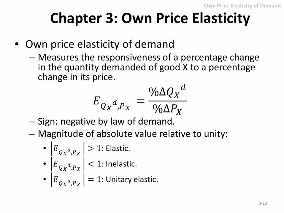
Chapter 3: Own Price Elasticity • Own price elasticity of demand

– Measures the responsiveness of a percentage change in the quantity demanded of good X to a percentage change in its price.

𝐸𝐸𝑄𝑄𝑋𝑋𝑑𝑑,𝑃𝑃𝑋𝑋 =%Δ𝑄𝑄𝑋𝑋𝑑𝑑

%Δ𝑃𝑃𝑋𝑋

– Sign: negative by law of demand. – Magnitude of absolute value relative to unity:

• 𝐸𝐸𝑄𝑄𝑋𝑋𝑑𝑑,𝑃𝑃𝑋𝑋 > 1: Elastic.

• 𝐸𝐸𝑄𝑄𝑋𝑋𝑑𝑑,𝑃𝑃𝑋𝑋 < 1: Inelastic.

• 𝐸𝐸𝑄𝑄𝑋𝑋𝑑𝑑,𝑃𝑃𝑋𝑋 = 1: Unitary elastic.

3-13

Own Price Elasticity of Demand

Chapter 3: Total Revenue Test • When demand is elastic:

– A price increase (decrease) leads to a decrease (increase) in total revenue.

• When demand is inelastic: – A price increase (decrease) leads to an increase

(decrease) in total revenue.

• When demand is unitary elastic: – Total revenue is maximized.

3-14

Own Price Elasticity of Demand

Chapter 3: Factors Affecting the Own Price Elasticity

• Three factors can impact the own price elasticity of demand: – Availability of consumption substitutes. – Time/Duration of purchase horizon. – Expenditure share of consumers’ budgets.

3-15

Own Price Elasticity of Demand

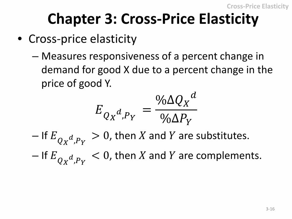
Chapter 3: Cross-Price Elasticity • Cross-price elasticity

– Measures responsiveness of a percent change in demand for good X due to a percent change in the price of good Y.

𝐸𝐸𝑄𝑄𝑋𝑋𝑑𝑑,𝑃𝑃𝑌𝑌 =%Δ𝑄𝑄𝑋𝑋𝑑𝑑

%Δ𝑃𝑃𝑌𝑌

– If 𝐸𝐸𝑄𝑄𝑋𝑋𝑑𝑑,𝑃𝑃𝑌𝑌 > 0, then 𝑋𝑋 and 𝑌𝑌 are substitutes.

– If 𝐸𝐸𝑄𝑄𝑋𝑋𝑑𝑑,𝑃𝑃𝑌𝑌 < 0, then 𝑋𝑋 and 𝑌𝑌 are complements.

3-16

Cross-Price Elasticity

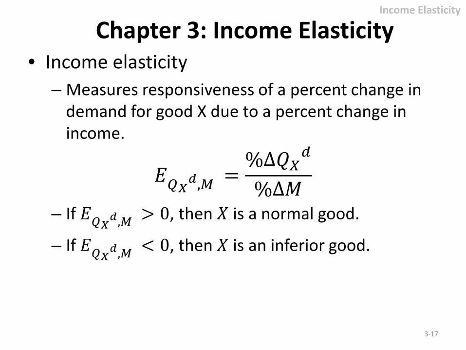
Chapter 3: Income Elasticity • Income elasticity

– Measures responsiveness of a percent change in demand for good X due to a percent change in income.

𝐸𝐸𝑄𝑄𝑋𝑋𝑑𝑑,𝑀𝑀 =%Δ𝑄𝑄𝑋𝑋𝑑𝑑

%Δ𝑀𝑀

– If 𝐸𝐸𝑄𝑄𝑋𝑋𝑑𝑑,𝑀𝑀 > 0, then 𝑋𝑋 is a normal good.

– If 𝐸𝐸𝑄𝑄𝑋𝑋𝑑𝑑,𝑀𝑀 < 0, then 𝑋𝑋 is an inferior good.

3-17

Income Elasticity

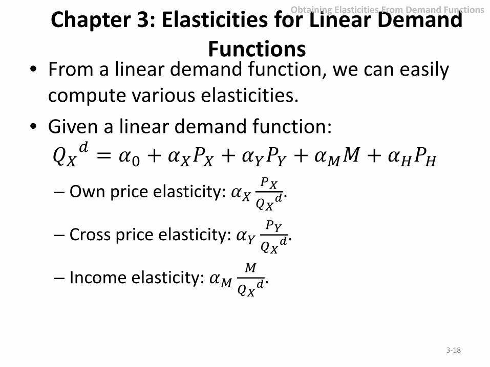
Chapter 3: Elasticities for Linear Demand Functions

• From a linear demand function, we can easily compute various elasticities.

• Given a linear demand function: 𝑄𝑄𝑋𝑋𝑑𝑑 = 𝛼𝛼0 + 𝛼𝛼𝑋𝑋𝑃𝑃𝑋𝑋 + 𝛼𝛼𝑌𝑌𝑃𝑃𝑌𝑌 + 𝛼𝛼𝑀𝑀𝑀𝑀 + 𝛼𝛼𝐻𝐻𝑃𝑃𝐻𝐻

– Own price elasticity: 𝛼𝛼𝑋𝑋𝑃𝑃𝑋𝑋𝑄𝑄𝑋𝑋𝑑𝑑

.

– Cross price elasticity: 𝛼𝛼𝑌𝑌𝑃𝑃𝑌𝑌𝑄𝑄𝑋𝑋𝑑𝑑

.

– Income elasticity: 𝛼𝛼𝑀𝑀𝑀𝑀𝑄𝑄𝑋𝑋𝑑𝑑

.

3-18

Obtaining Elasticities From Demand Functions

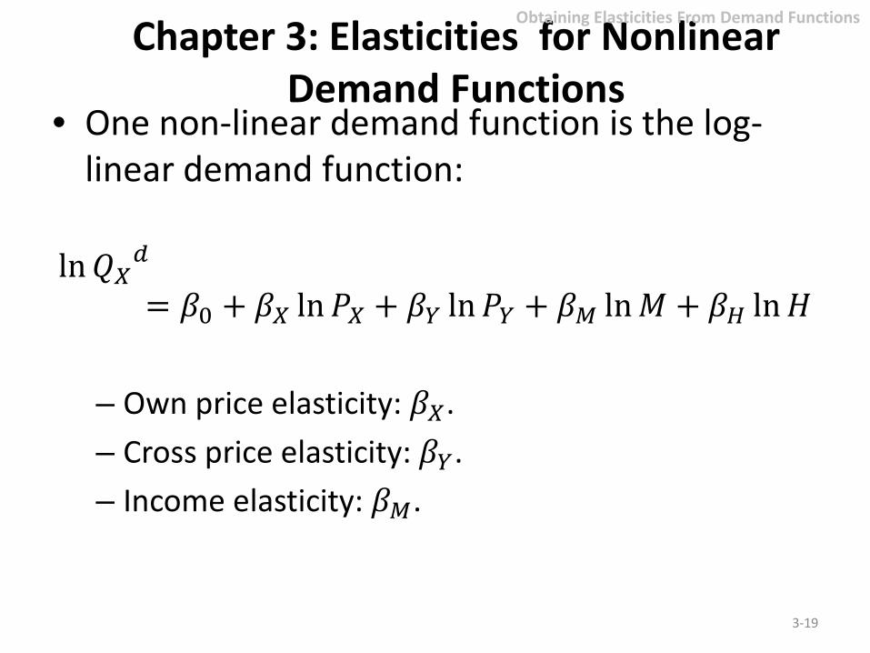
Chapter 3: Elasticities for Nonlinear Demand Functions

• One non-linear demand function is the log-linear demand function:

ln𝑄𝑄𝑋𝑋𝑑𝑑

= 𝛽𝛽0 + 𝛽𝛽𝑋𝑋 ln𝑃𝑃𝑋𝑋 + 𝛽𝛽𝑌𝑌 ln𝑃𝑃𝑌𝑌 + 𝛽𝛽𝑀𝑀 ln𝑀𝑀 + 𝛽𝛽𝐻𝐻 ln𝐻𝐻 – Own price elasticity: 𝛽𝛽𝑋𝑋. – Cross price elasticity: 𝛽𝛽𝑌𝑌. – Income elasticity: 𝛽𝛽𝑀𝑀.

3-19

Obtaining Elasticities From Demand Functions

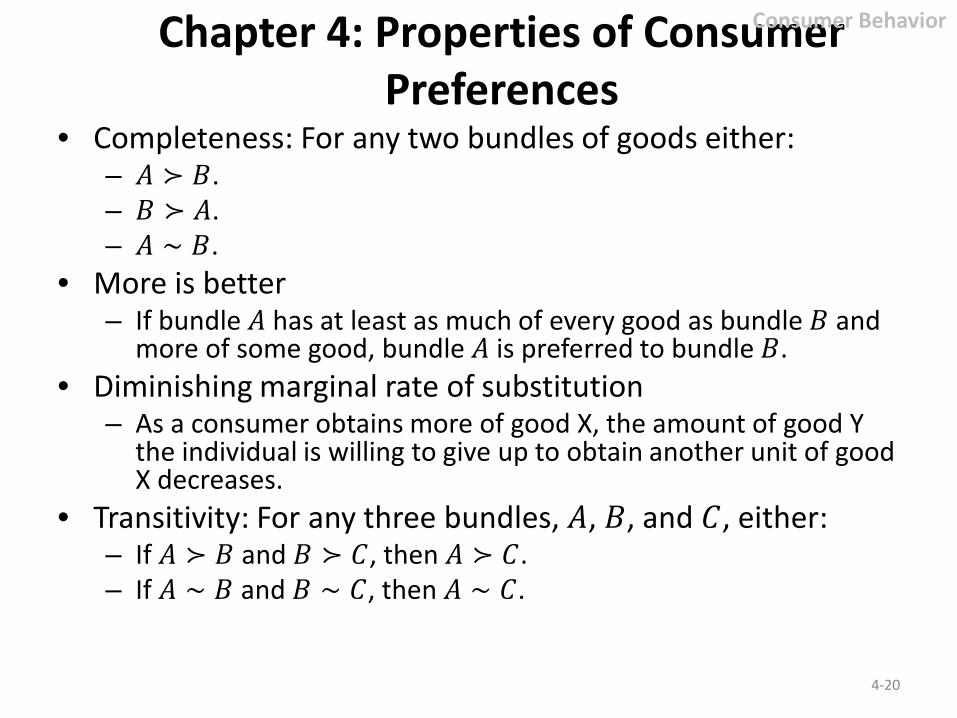
Chapter 4: Properties of Consumer Preferences

• Completeness: For any two bundles of goods either: – 𝐴𝐴 ≻ 𝑀𝑀. – 𝑀𝑀 ≻ 𝐴𝐴. – 𝐴𝐴 ∼ 𝑀𝑀.

• More is better – If bundle 𝐴𝐴 has at least as much of every good as bundle 𝑀𝑀 and

more of some good, bundle 𝐴𝐴 is preferred to bundle 𝑀𝑀. • Diminishing marginal rate of substitution

– As a consumer obtains more of good X, the amount of good Y the individual is willing to give up to obtain another unit of good X decreases.

• Transitivity: For any three bundles, 𝐴𝐴, 𝑀𝑀, and 𝐶𝐶, either: – If 𝐴𝐴 ≻ 𝑀𝑀 and 𝑀𝑀 ≻ 𝐶𝐶, then 𝐴𝐴 ≻ 𝐶𝐶. – If 𝐴𝐴 ∼ 𝑀𝑀 and 𝑀𝑀 ∼ 𝐶𝐶, then 𝐴𝐴 ∼ 𝐶𝐶.

4-20

Consumer Behavior

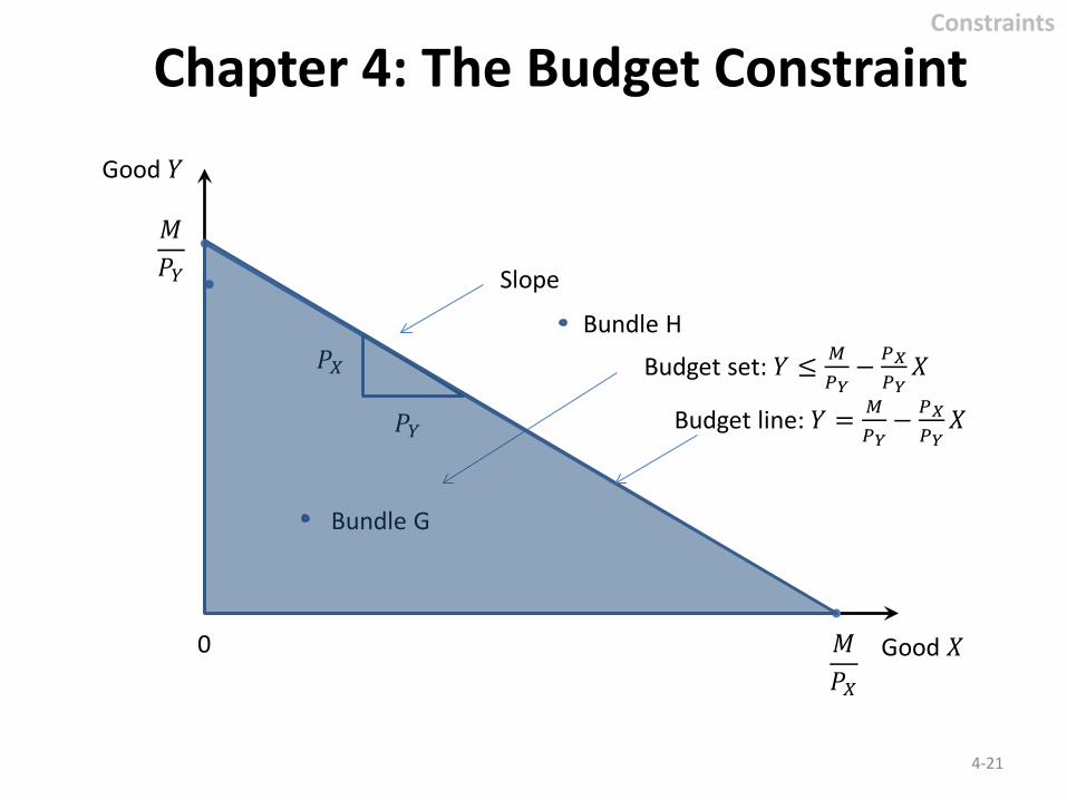
Chapter 4: The Budget Constraint

4-21

Good 𝑋𝑋

Good 𝑌𝑌

0

Budget line: 𝑌𝑌 = 𝑀𝑀𝑃𝑃𝑌𝑌− 𝑃𝑃𝑋𝑋

𝑃𝑃𝑌𝑌𝑋𝑋

𝑀𝑀𝑃𝑃𝑌𝑌

𝑀𝑀𝑃𝑃𝑋𝑋

𝑃𝑃𝑋𝑋

𝑃𝑃𝑌𝑌

Slope

Bundle G

Bundle H

Budget set: 𝑌𝑌 ≤ 𝑀𝑀𝑃𝑃𝑌𝑌− 𝑃𝑃𝑋𝑋

𝑃𝑃𝑌𝑌𝑋𝑋

Constraints

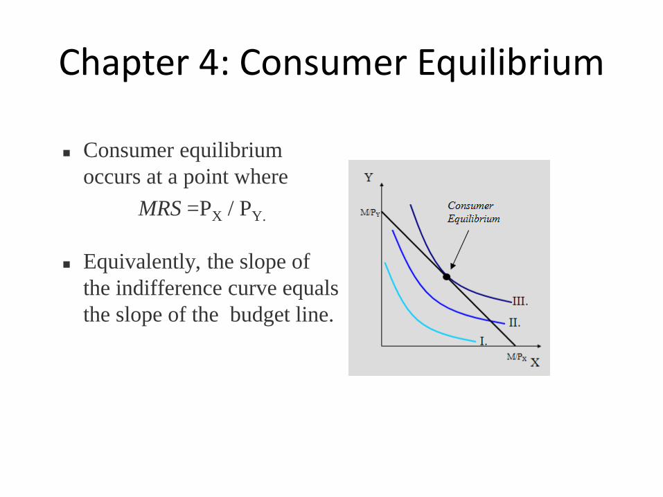
Chapter 4: Consumer Equilibrium

Consumer equilibrium occurs at a point where

MRS =PX / PY.

Equivalently, the slope of the indifference curve equals the slope of the budget line.

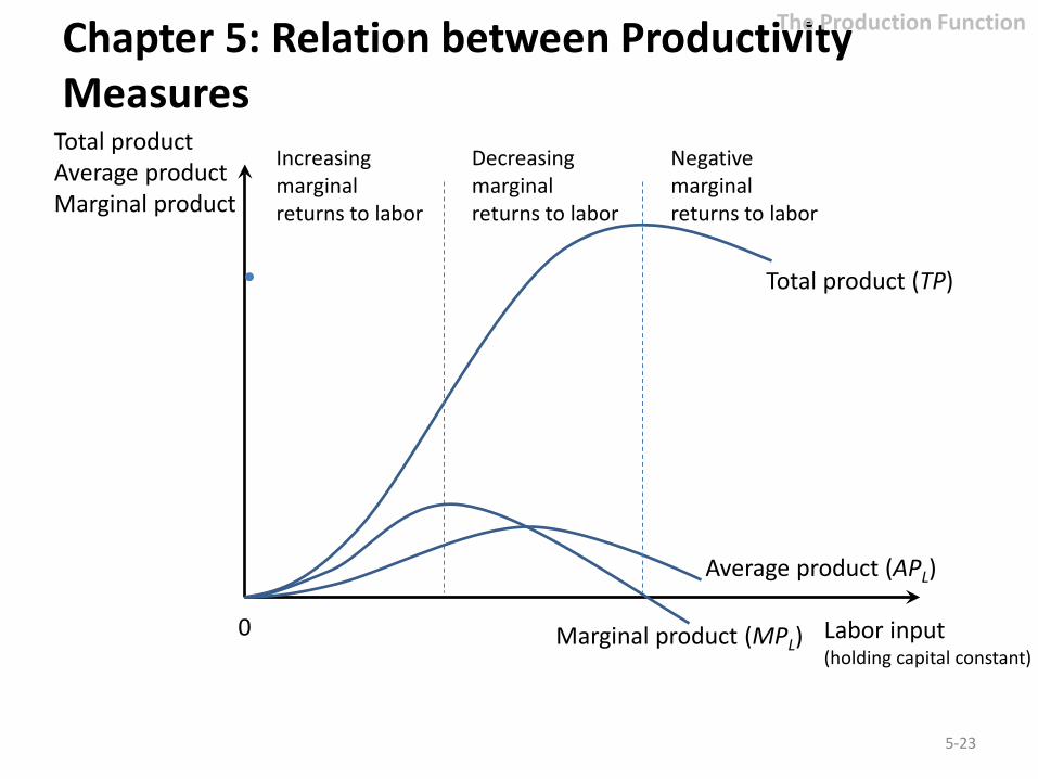
Chapter 5: Relation between Productivity Measures

5-23

Labor input (holding capital constant)

0

Total product Average product Marginal product

Total product (TP)

Average product (APL)

Marginal product (MPL)

Increasing marginal returns to labor

Decreasing marginal returns to labor

Negative marginal returns to labor

The Production Function

Chapter 5: Profit Maximizing Input Usage

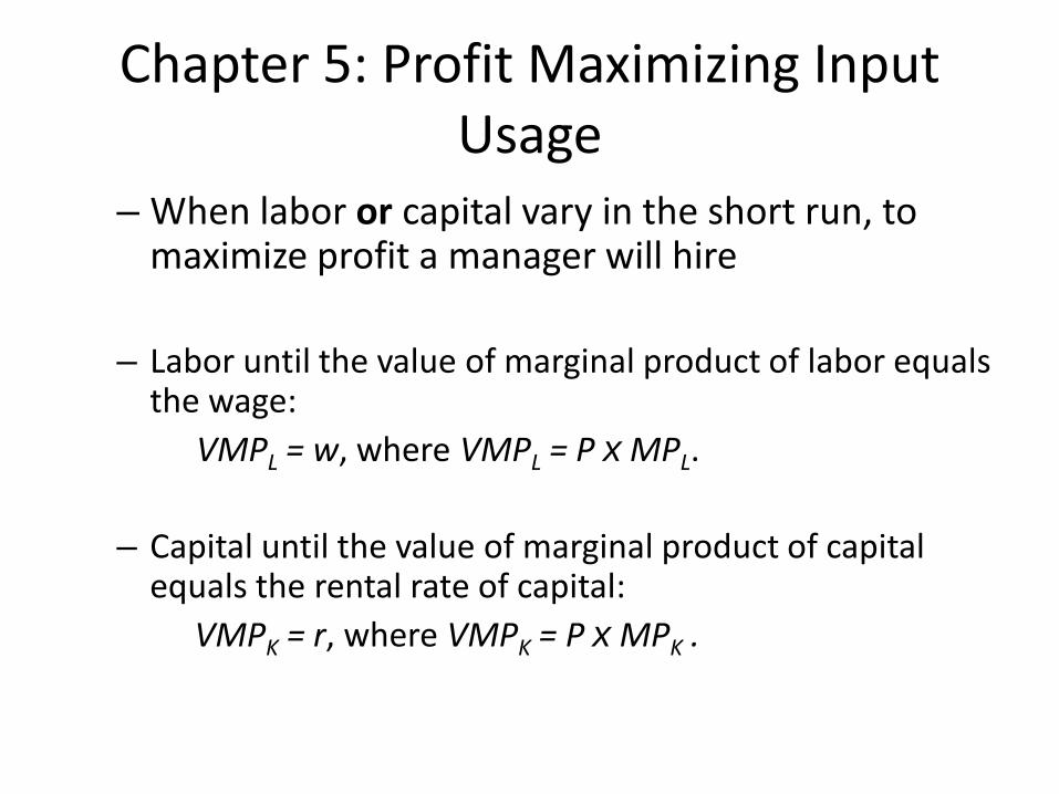
– When labor or capital vary in the short run, to maximize profit a manager will hire

– Labor until the value of marginal product of labor equals the wage:

VMPL = w, where VMPL = P x MPL.

– Capital until the value of marginal product of capital equals the rental rate of capital:

VMPK = r, where VMPK = P x MPK .

Chapter 5: Isoquants and Marginal Rate of Technical Substitution

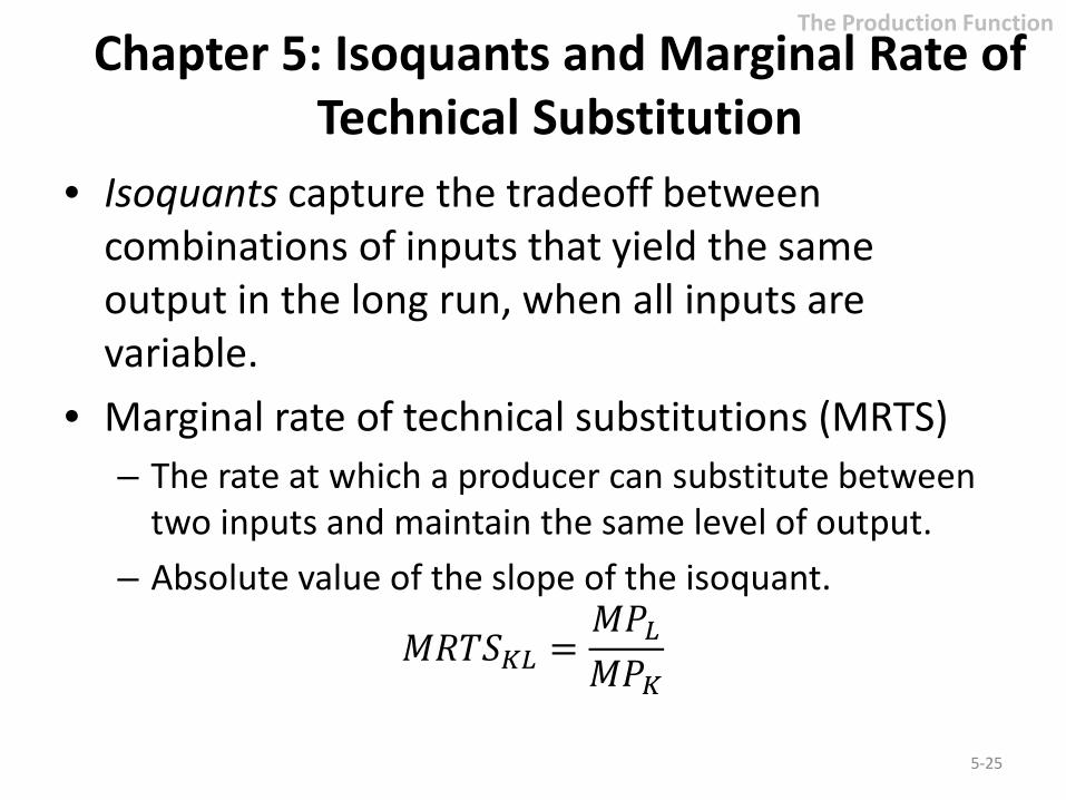
• Isoquants capture the tradeoff between combinations of inputs that yield the same output in the long run, when all inputs are variable.

• Marginal rate of technical substitutions (MRTS) – The rate at which a producer can substitute between

two inputs and maintain the same level of output. – Absolute value of the slope of the isoquant.

𝑀𝑀𝑀𝑀𝑀𝑀𝑀𝑀𝐾𝐾𝐾𝐾 =𝑀𝑀𝑃𝑃𝐾𝐾𝑀𝑀𝑃𝑃𝐾𝐾

5-25

The Production Function

Chapter 5: Cost Minimization

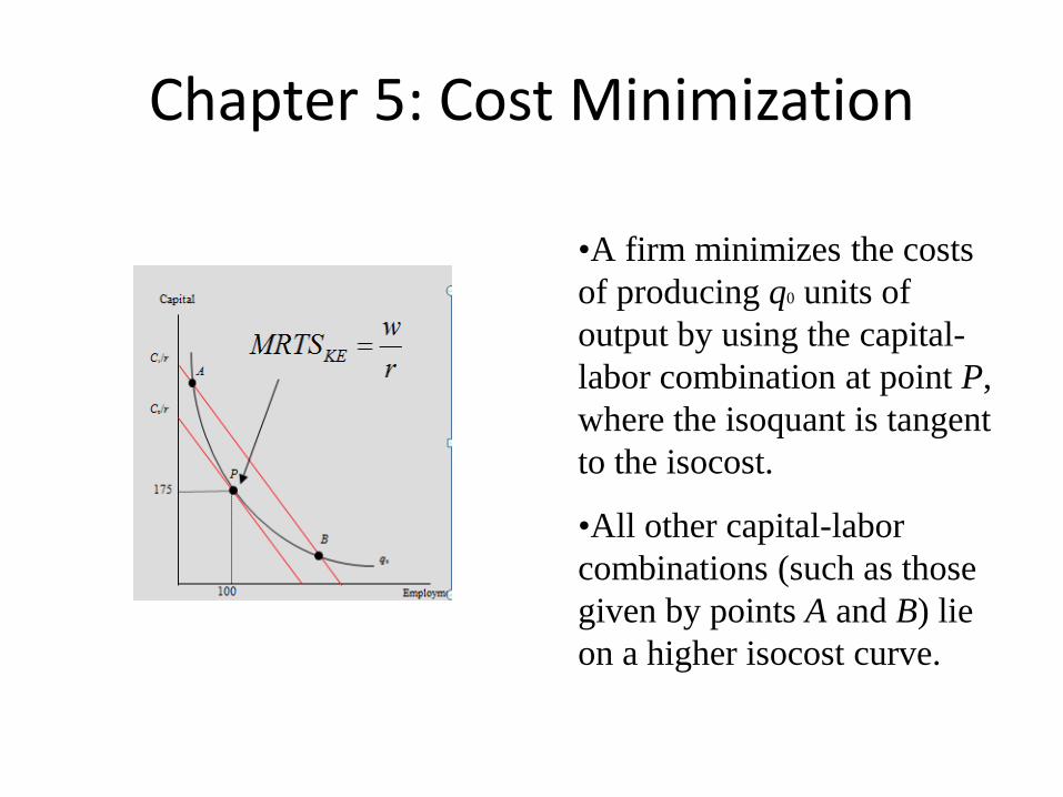
•A firm minimizes the costs of producing q0 units of output by using the capital-labor combination at point P, where the isoquant is tangent to the isocost.

•All other capital-labor combinations (such as those given by points A and B) lie on a higher isocost curve.

Chapter 5: Cost Minimization

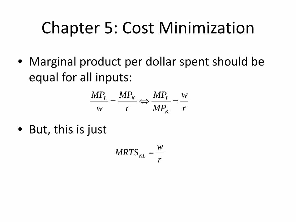
• Marginal product per dollar spent should be equal for all inputs:

• But, this is just

rw

MPMP

rMP

wMP

K

LKL =⇔=

rwMRTSKL =

Chapter 5: The Cost Function • Mathematical relationship that relates cost to the

cost-minimizing output associated with an isoquant.

• Short-run costs – Fixed costs: 𝐹𝐹𝐶𝐶 – Sunk costs – Short-run variable costs: 𝑉𝑉𝐶𝐶 𝑄𝑄 – Short-run total costs: 𝑀𝑀𝐶𝐶 𝑄𝑄 = 𝐹𝐹𝐶𝐶 + 𝑉𝑉𝐶𝐶 𝑄𝑄

• Long-run costs – All costs are variable – No fixed costs

5-28

The Cost Function

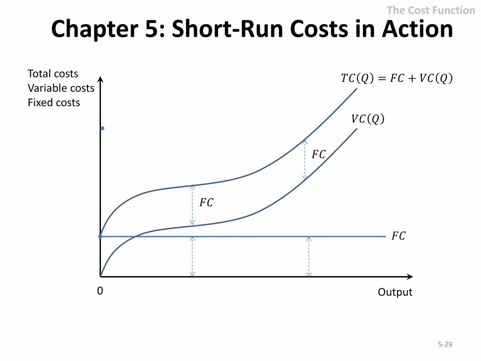
Chapter 5: Short-Run Costs in Action

5-29

Output 0

𝑀𝑀𝐶𝐶 𝑄𝑄 = 𝐹𝐹𝐶𝐶 + 𝑉𝑉𝐶𝐶 𝑄𝑄

𝑉𝑉𝐶𝐶 𝑄𝑄

𝐹𝐹𝐶𝐶

𝐹𝐹𝐶𝐶

Total costs Variable costs Fixed costs

𝐹𝐹𝐶𝐶

The Cost Function

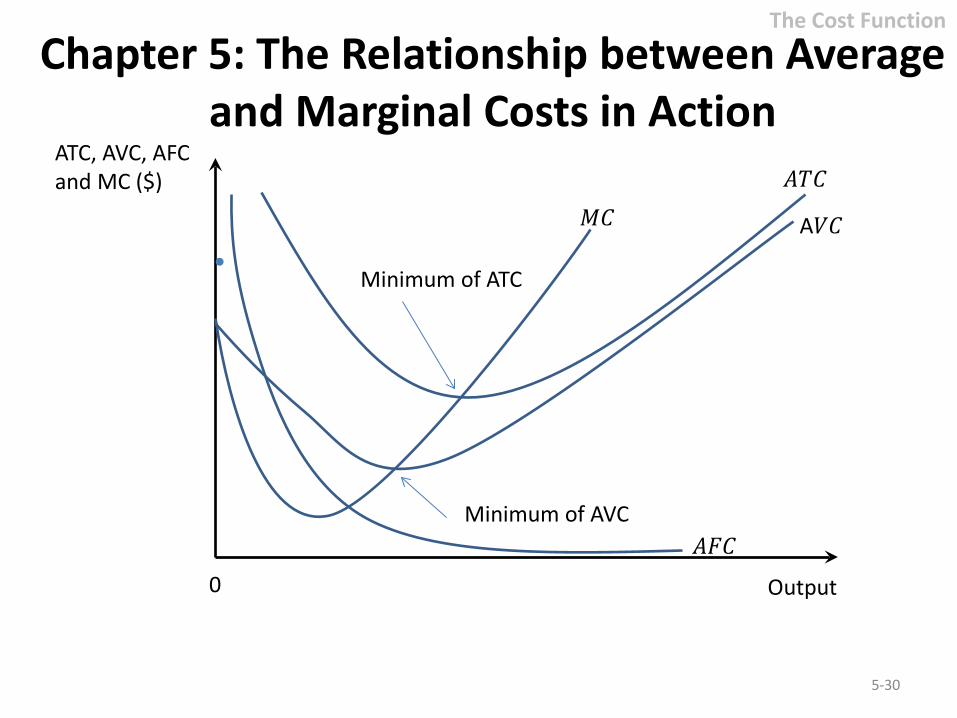
Chapter 5: The Relationship between Average and Marginal Costs in Action

5-30

Output 0

𝐴𝐴𝑀𝑀𝐶𝐶

A𝑉𝑉𝐶𝐶 𝑀𝑀𝐶𝐶

ATC, AVC, AFC and MC ($)

𝐴𝐴𝐹𝐹𝐶𝐶

Minimum of ATC

Minimum of AVC

The Cost Function

Chapter 5: Economies of Scale • Economies of scale

– Portion of the long-run average cost curve where long-run average costs decline as output increases.

• Diseconomies of scale – Portion of the long-run average cost curve where

long-run average costs increase as output increases.

• Constant returns to scale – Portion of the long-run average cost curve that

remains constant as output increases.

5-31

The Cost Function

Chapter 5: Multiple-Output Cost Function

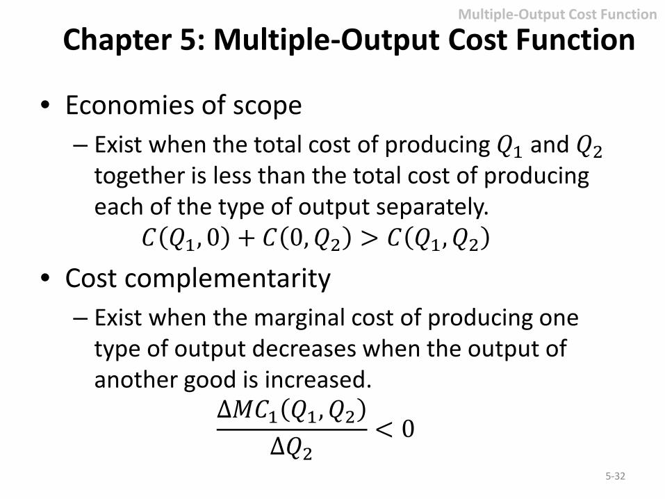
• Economies of scope – Exist when the total cost of producing 𝑄𝑄1 and 𝑄𝑄2

together is less than the total cost of producing each of the type of output separately.

𝐶𝐶 𝑄𝑄1, 0 + 𝐶𝐶 0,𝑄𝑄2 > 𝐶𝐶 𝑄𝑄1,𝑄𝑄2

• Cost complementarity – Exist when the marginal cost of producing one

type of output decreases when the output of another good is increased.

∆𝑀𝑀𝐶𝐶1 𝑄𝑄1,𝑄𝑄2∆𝑄𝑄2

< 0

5-32

Multiple-Output Cost Function

Chapter 8: Perfect Competition • To maximize short-run profits, a perfectly

competitive firm should produce in the range of increasing marginal cost where 𝑃𝑃 = 𝑀𝑀𝐶𝐶, provided that 𝑃𝑃 ≥ 𝐴𝐴𝑉𝑉𝐶𝐶. If 𝑃𝑃 < 𝐴𝐴𝑉𝑉𝐶𝐶, the firm should shut down its plant to minimize it losses.

8-33

Perfect Competition

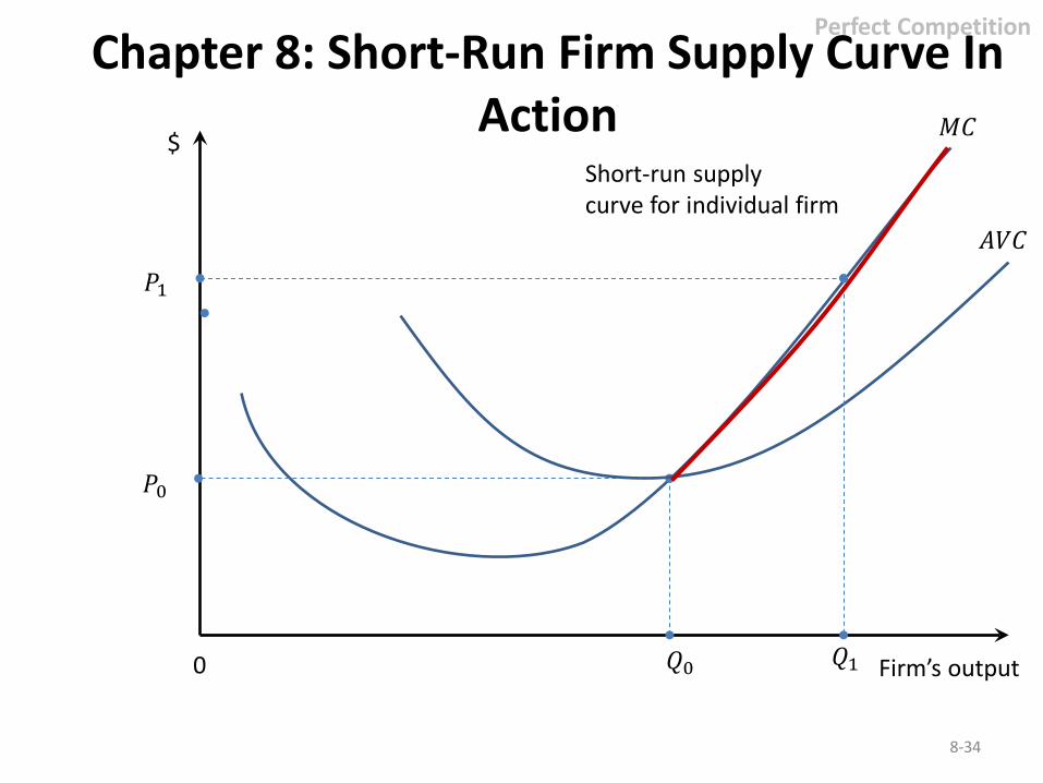
Chapter 8: Short-Run Firm Supply Curve In Action

8-34

Perfect Competition

Firm’s output

$

0 𝑄𝑄0

𝑃𝑃0

𝑀𝑀𝐶𝐶

𝐴𝐴𝑉𝑉𝐶𝐶

𝑃𝑃1

𝑄𝑄1

Short-run supply curve for individual firm

Chapter 8: Long-Run Competitive Equilibrium

• In the long run, perfectly competitive firms produce a level of output such that 𝑃𝑃 = 𝑀𝑀𝐶𝐶 𝑃𝑃 = 𝑚𝑚𝑚𝑚𝑚𝑚𝑚𝑚𝑚𝑚𝑚𝑚𝑚𝑚 𝑜𝑜𝑜𝑜 𝐴𝐴𝐶𝐶

8-35

Perfect Competition

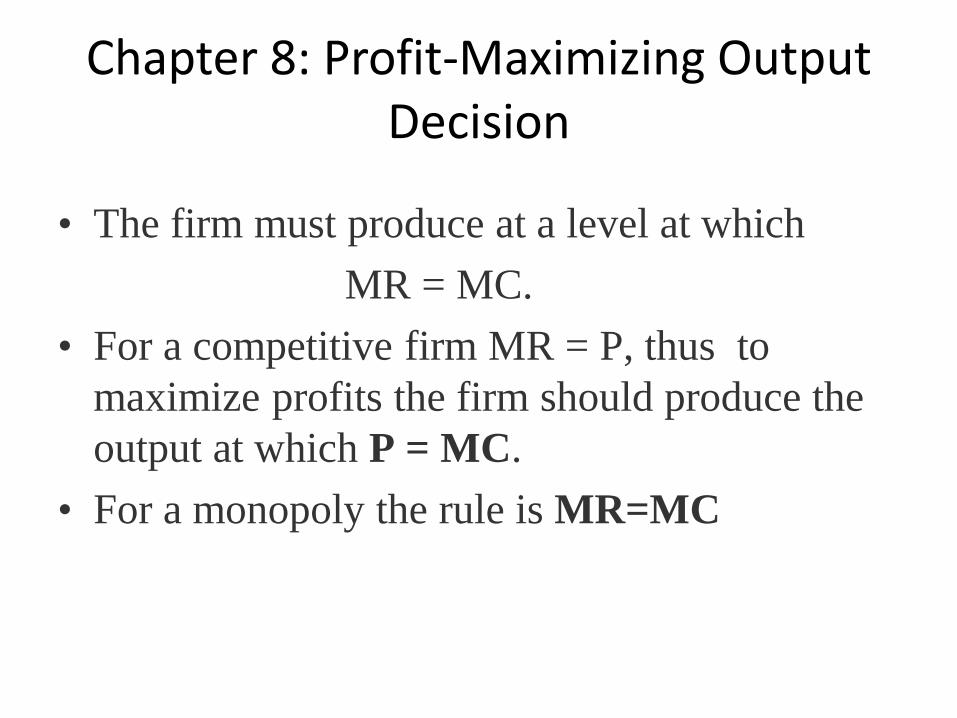
Chapter 8: Profit-Maximizing Output Decision

• The firm must produce at a level at which MR = MC. • For a competitive firm MR = P, thus to

maximize profits the firm should produce the output at which P = MC.

• For a monopoly the rule is MR=MC

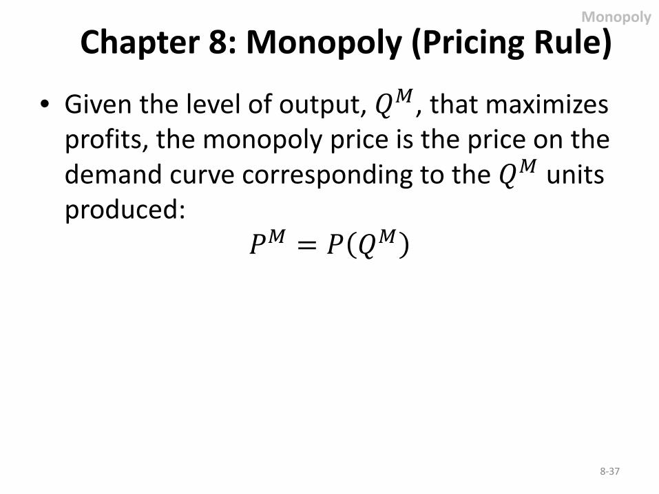
Chapter 8: Monopoly (Pricing Rule)

• Given the level of output, 𝑄𝑄𝑀𝑀, that maximizes profits, the monopoly price is the price on the demand curve corresponding to the 𝑄𝑄𝑀𝑀 units produced:

𝑃𝑃𝑀𝑀 = 𝑃𝑃 𝑄𝑄𝑀𝑀

8-37

Monopoly

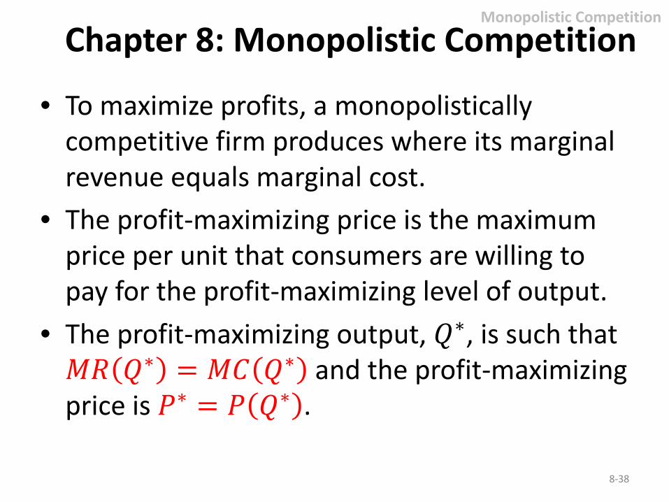
Chapter 8: Monopolistic Competition

• To maximize profits, a monopolistically competitive firm produces where its marginal revenue equals marginal cost.

• The profit-maximizing price is the maximum price per unit that consumers are willing to pay for the profit-maximizing level of output.

• The profit-maximizing output, 𝑄𝑄∗, is such that 𝑀𝑀𝑀𝑀 𝑄𝑄∗ = 𝑀𝑀𝐶𝐶 𝑄𝑄∗ and the profit-maximizing price is 𝑃𝑃∗ = 𝑃𝑃 𝑄𝑄∗ .

8-38

Monopolistic Competition

Price

Quantity of Brand X

MC

𝑄𝑄∗

𝑃𝑃∗

ATC

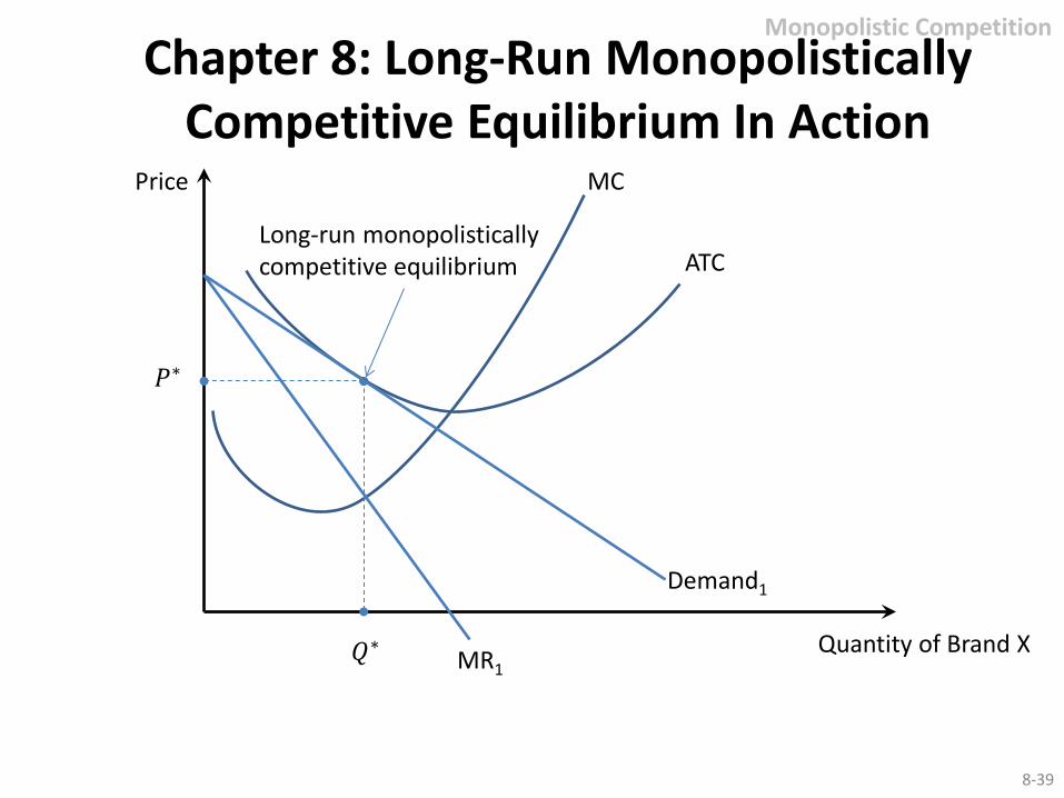
Chapter 8: Long-Run Monopolistically Competitive Equilibrium In Action

Monopolistic Competition

8-39

Demand1

MR1

Long-run monopolistically competitive equilibrium

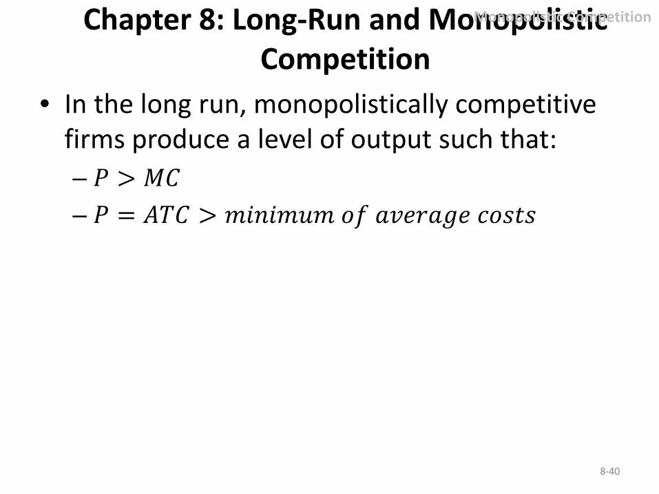
Chapter 8: Long-Run and Monopolistic Competition

• In the long run, monopolistically competitive firms produce a level of output such that: – 𝑃𝑃 > 𝑀𝑀𝐶𝐶 – 𝑃𝑃 = 𝐴𝐴𝑀𝑀𝐶𝐶 > 𝑚𝑚𝑚𝑚𝑚𝑚𝑚𝑚𝑚𝑚𝑚𝑚𝑚𝑚 𝑜𝑜𝑜𝑜 𝑎𝑎𝑎𝑎𝑎𝑎𝑎𝑎𝑎𝑎𝑎𝑎𝑎𝑎 𝑐𝑐𝑜𝑜𝑐𝑐𝑐𝑐𝑐𝑐

8-40

Monopolistic Competition

Chapter 9: Basic Oligopoly

• Profit Maximization in Four Oligopoly Settings

– Cournot Model – Stackelberg Model – Bertrand Model – Collusion

Chapter 9

• Different oligopoly scenarios give rise to different optimal strategies and different outcomes.

• Your optimal price and output depends on … – Beliefs about the reactions of rivals. – Your choice variable (P or Q) and the nature of the

product market (differentiated or homogeneous products).

– Your ability to credibly commit prior to your rivals.

9-42

Chapter 10 Game Theory

• Game theory is the study of how people behave in strategic situations.

• Strategic decisions are those in which each person, in deciding what actions to take, must consider how others might respond to that action.

Copyright © 2014 by the McGraw-Hill Companies, Inc. All rights reserved. 2-43

What is a Game?

• A game is a situation where the participants’ payoffs depend not only on their decisions, but also on their rivals’ decisions.

i.e. My optimal decisions will depend on what others do in the game.

Copyright © 2014 by the McGraw-Hill Companies, Inc. All rights reserved. 2-44

Elements to describe a game

• A set of players • A set of actions- action or strategy set for

each player • Payoffs – ranking of the possible outcomes

Copyright © 2014 by the McGraw-Hill Companies, Inc. All rights reserved. 2-45

Forms

• Strategic Form (Normal Form) • Extensive Form (Game Tree)

Copyright © 2014 by the McGraw-Hill Companies, Inc. All rights reserved. 2-46

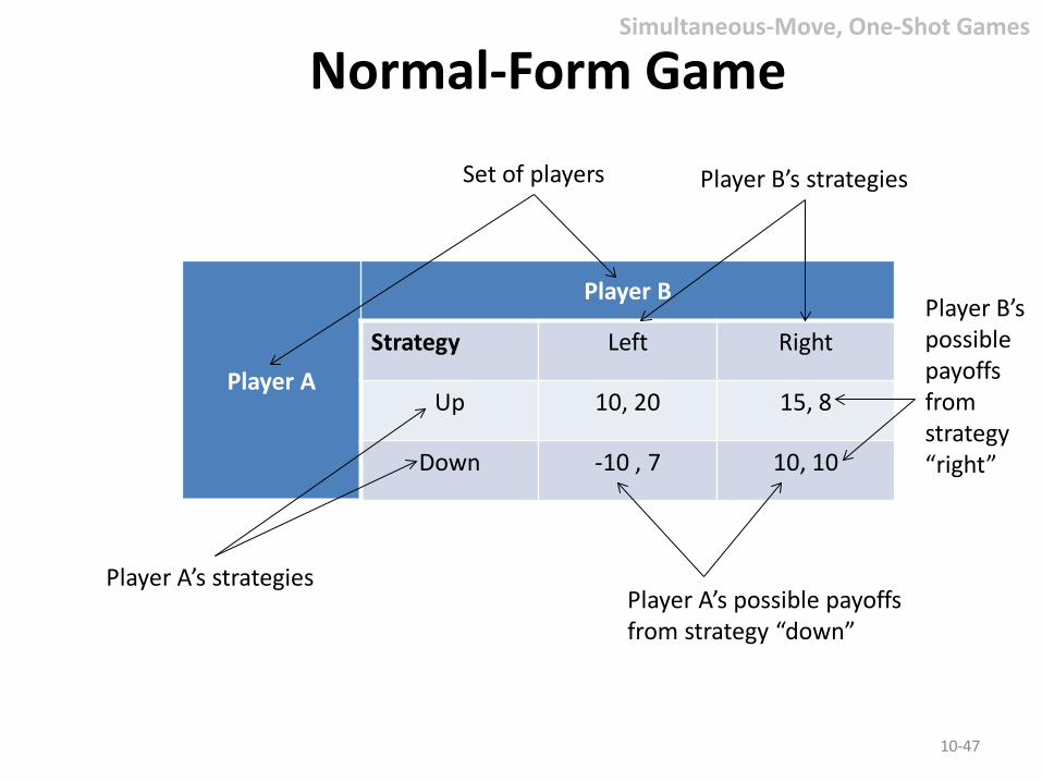
Normal-Form Game

10-47

Simultaneous-Move, One-Shot Games

Player A

Player B

Strategy Left Right

Up 10, 20 15, 8

Down -10 , 7 10, 10

Set of players

Player A’s strategies

Player B’s strategies

Player A’s possible payoffs from strategy “down”

Player B’s possible payoffs from strategy “right”

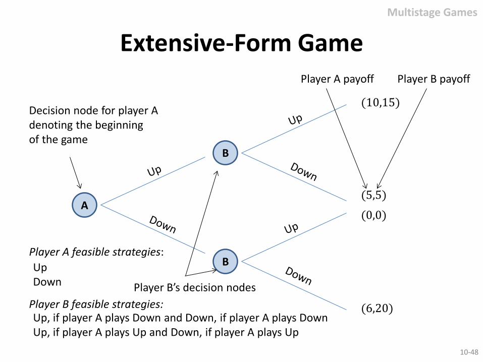
Extensive-Form Game Multistage Games

B

B

A

(10,15)

(5,5)

(0,0)

(6,20)

Decision node for player A denoting the beginning of the game

Player B’s decision nodes

Player A payoff Player B payoff

Player A feasible strategies:

Player B feasible strategies:

Up Down

Up, if player A plays Down and Down, if player A plays Down Up, if player A plays Up and Down, if player A plays Up

10-48

Possible Strategies • Dominant strategy

– A strategy that results in the highest payoff to a player regardless of the opponent’s action.

• Nash equilibrium strategy – A condition describing a set of strategies in which

no player can improve her payoff by unilaterally changing her own strategy, given the other players’ strategies.

10-49

Simultaneous-Move, One-Shot Games