UNIVERSITY OF MANCHESTER

Mandelbrot on FPGA

by

Obaya Dralega

A thesis submitted in partial fulfillment for the

degree of Bachelor of Science

in the

School of Computer Science

May 2016

UNIVERSITY OF MANCHESTER

Abstract

School of Computer Science

Bachelor of Science

by Obaya Dralega

The Mandelbrot Set is one of the most popular fractal images today. The term fractal

is applied to mathematically defined shapes or objects that display self-similarity at

various scales. Although mathematically defined, fractal shapes are often seen in the

natural world, from trees to clouds to coastlines.

FPGAs (Field Programmable Gate Arrays) are computing devices composed of config-

urable logic blocks connected by a programmable Interconnection Fabric. An FPGA

is able to be reprogrammed to implement any digital circuit with its capacity. This

means that an FPGA is able to implement a Hardware overlay, which is an FPGA

implementation of an existing processor architecture.

This project report follows the progress in the research, development and implementation

of a system for the computation of the image of the Mandelbrot set on an FPGA Overlay.

Due to several unforeseeable delays to my progress, as well as a steep learning curve,

I was unable to implement my final design on an FPGA, although I proved my design

functionally correct through a software implementation and simulation. Screen-shots of

my software results are presented along with a summary of the implementation details

of my design.

Acknowledgements

I would like to thank my supervisor, Dr. Dirk Koch for his endless enthusiasm and

invaluable advice.

ii

Contents

Abstract i

Acknowledgements ii

List of Figures v

1 Introduction 1

1.1 Mandelbrot Set . . . . . . . . . . . . . . . . . . . . . . . . . . . . . . . . . 1

1.1.1 Mathematical Description of the Mandelbrot Set . . . . . . . . . . 2

1.1.2 Computation of the Mandelbrot Set . . . . . . . . . . . . . . . . . 3

1.1.3 Zooming into the Mandelbrot Set . . . . . . . . . . . . . . . . . . . 4

1.1.4 Computational considerations when Computing the Mandelbrot Set 5

1.1.4.1 Finite Resolution . . . . . . . . . . . . . . . . . . . . . . . 5

1.1.4.2 Accuracy versus Time . . . . . . . . . . . . . . . . . . . . 5

1.2 FPGA . . . . . . . . . . . . . . . . . . . . . . . . . . . . . . . . . . . . . . 6

1.2.1 FPGA Architecture . . . . . . . . . . . . . . . . . . . . . . . . . . 6

1.2.2 Why use FPGAs ? . . . . . . . . . . . . . . . . . . . . . . . . . . . 7

1.2.2.1 Mandelbrot and FPGAs . . . . . . . . . . . . . . . . . . . 8

1.2.3 Hardware Platform . . . . . . . . . . . . . . . . . . . . . . . . . . . 8

1.3 FPGA Programming . . . . . . . . . . . . . . . . . . . . . . . . . . . . . . 9

1.3.1 Hardware Description Languages . . . . . . . . . . . . . . . . . . . 9

1.3.2 Schematic Design . . . . . . . . . . . . . . . . . . . . . . . . . . . . 9

1.3.3 Hardware Overlays . . . . . . . . . . . . . . . . . . . . . . . . . . . 9

1.4 MIPS Architecture . . . . . . . . . . . . . . . . . . . . . . . . . . . . . . . 11

1.4.1 MIPS Functional Blocks . . . . . . . . . . . . . . . . . . . . . . . . 11

1.4.2 MIPS Instruction Set . . . . . . . . . . . . . . . . . . . . . . . . . 12

1.5 Number Representations . . . . . . . . . . . . . . . . . . . . . . . . . . . . 14

1.5.1 Floating Point . . . . . . . . . . . . . . . . . . . . . . . . . . . . . 14

1.5.2 Fixed Point . . . . . . . . . . . . . . . . . . . . . . . . . . . . . . . 14

2 Design and Implementation 16

2.1 System Implementation Overview . . . . . . . . . . . . . . . . . . . . . . . 16

2.2 Mandelbrot C code . . . . . . . . . . . . . . . . . . . . . . . . . . . . . . . 17

2.3 Complex Number C code . . . . . . . . . . . . . . . . . . . . . . . . . . . 17

2.4 Fixed Point Code . . . . . . . . . . . . . . . . . . . . . . . . . . . . . . . . 19

iii

Contents iv

2.4.1 Comparison of Fixed and Floating Point Representations for Man-delbrot . . . . . . . . . . . . . . . . . . . . . . . . . . . . . . . . . 19

2.4.2 Scale Factor . . . . . . . . . . . . . . . . . . . . . . . . . . . . . . . 20

2.4.2.1 Effect of varying the Scale Factor . . . . . . . . . . . . . 20

2.4.3 Conversion . . . . . . . . . . . . . . . . . . . . . . . . . . . . . . . 22

2.5 Cross Compilation . . . . . . . . . . . . . . . . . . . . . . . . . . . . . . . 23

2.5.1 Building the Cross Compiler Toolchain . . . . . . . . . . . . . . . . 23

2.6 Effects of Number of Iterations on Image Quality . . . . . . . . . . . . . . 24

3 Evaluation 26

3.1 Code Evaluation . . . . . . . . . . . . . . . . . . . . . . . . . . . . . . . . 26

3.2 Simulation . . . . . . . . . . . . . . . . . . . . . . . . . . . . . . . . . . . . 27

4 Reflections and Conclusion 29

4.1 Change of Objective . . . . . . . . . . . . . . . . . . . . . . . . . . . . . . 29

4.2 Challenges . . . . . . . . . . . . . . . . . . . . . . . . . . . . . . . . . . . . 29

4.3 Conclusion . . . . . . . . . . . . . . . . . . . . . . . . . . . . . . . . . . . 30

5 Further Research 31

5.1 The Mandelbulb . . . . . . . . . . . . . . . . . . . . . . . . . . . . . . . . 31

5.1.1 Changes to be Made . . . . . . . . . . . . . . . . . . . . . . . . . 32

A Run Away to Infinity Criterion 33

Bibliography 35

List of Figures

1.1 The full Mandelbrot set image. . . . . . . . . . . . . . . . . . . . . . . . . 1

1.2 A complex number can be visually represented as a pair of numbers form-ing a vector on a diagram called an Argand diagram, representing thecomplex plane. . . . . . . . . . . . . . . . . . . . . . . . . . . . . . . . . . 2

1.3 A visual representation of the magnitude of a complex number. . . . . . . 3

1.4 A zoom into a section of the Mandelbrot set. . . . . . . . . . . . . . . . . 4

1.5 A diagram showing how the centre points of pixels are chosen from a finitepixel array to represent complex numbers [3]. . . . . . . . . . . . . . . . . 5

1.6 Generic FPGA Logic Element [5]. . . . . . . . . . . . . . . . . . . . . . . . 6

1.7 Generic Island Style FPGA Architecture [5]. . . . . . . . . . . . . . . . . . 7

1.8 The Xilinx Nexys 4 DDR FPGA Board [11]. . . . . . . . . . . . . . . . . . 8

1.9 Overview of the MIPS functional components [18]. . . . . . . . . . . . . . 12

1.10 MIPS instruction types [18] . . . . . . . . . . . . . . . . . . . . . . . . . . 13

1.11 How floating point numbers are represented at the bit level [22]. . . . . . 14

1.12 How fixed point numbers are represented at the bit level [23] . . . . . . . 15

2.1 A diagram giving a high-level design overview of the system. . . . . . . . 16

2.2 Mandelbrot render with scale factor 4. . . . . . . . . . . . . . . . . . . . . 21

2.3 Mandelbrot render with scale factor 8. . . . . . . . . . . . . . . . . . . . . 21

2.4 Mandelbrot render with scale factor 24. . . . . . . . . . . . . . . . . . . . 21

2.5 Macros for handling fixed point numbers. . . . . . . . . . . . . . . . . . . 22

2.6 Unmodified main loop body of Mandelbrot computation using floatingpoint numbers. . . . . . . . . . . . . . . . . . . . . . . . . . . . . . . . . . 22

2.7 Modified main loop body of Mandelbrot computation using fixed pointnumbers. . . . . . . . . . . . . . . . . . . . . . . . . . . . . . . . . . . . . 22

2.8 A magnified section of the Mandelbrot set image computed using an in-creasing number of maximum of iterations. . . . . . . . . . . . . . . . . . 25

3.1 A screen shot of the some of the cross-compiled assembly code in the theInstruction BRAM of the MIPS overlay. . . . . . . . . . . . . . . . . . . . 27

3.2 A screen shot showing the button which launches the simulator afterchecking the Behavioural Syntax. . . . . . . . . . . . . . . . . . . . . . . . 27

3.3 A screen shot of the simulation window. . . . . . . . . . . . . . . . . . . 28

3.4 A close up screen shot of the most relevant signals in the simulation. . . . 28

5.1 A render of the Mandelbulb [31]. . . . . . . . . . . . . . . . . . . . . . . . 31

v

Dedicated to my parents, Audrey and Anguyo Dralega.

vi

Chapter 1

Introduction

This chapter will introduce the key concepts that are needed to understand the technical

details of the project and describe the project in a broad context.

1.1 Mandelbrot Set

The Mandelbrot Set is a fractal named after the mathematician Benoit Mandelbrot.

Fractals are objects that display self-similarity at various scales [1]. Magnifying a frac-

tal reveals small-scale details similar to the large-scale characteristics. Although the

Mandelbrot set is self-similar at magnified scales, the small scale details are not iden-

tical to the whole. In fact, the Mandelbrot set is infinitely complex, yet the process of

generating it is based on a simple equation involving complex numbers.

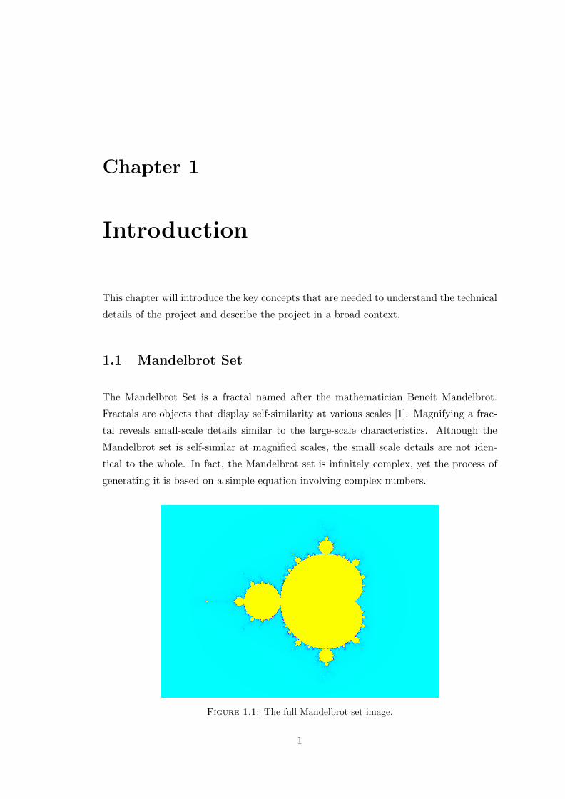
Figure 1.1: The full Mandelbrot set image.

1

Introduction 2

From a philosophical perspective, the Mandelbrot set challenges familiar notions of sim-

plicity and complexity: how could such a simple formula, involving only multiplication

and addition, produce a shape of great organic beauty and infinite subtle variation? It

defies conventional intuition and has captured the imagination of Computer Scientists

and Mathematicians for decades.

1.1.1 Mathematical Description of the Mandelbrot Set

The Mandelbrot set is mathematically defined as the set of complex numbers for which

the sequence zn+1 = z2n + c does not approach infinity when applied iteratively [2].

znn+ 1 = z2n + c

c ∈M ⇐⇒ limn→∞

|zn+1| ≤ 2

Complex numbers consist of a real number added to an imaginary number. While real

numbers can be represented on one dimensional number line, complex numbers have

two parts, so they are represented on a 2-dimensional plane called the complex number

plane or Argand diagram as can be seen below.

ComplexNumber : z = x+ yi

Figure 1.2: A complex number can be visually represented as a pair of numbersforming a vector on a diagram called an Argand diagram, representing the complex

plane.

Introduction 3

1.1.2 Computation of the Mandelbrot Set

To compute the Mandelbrot set we need to calculate which pixels of the display belong

to the set, we do this by applying the formula, zn+1 = z2n + c iteratively to each pixel.

We start with z0 = 0 and c takes its value from the co-ordinates of the pixel in the

complex plane.

When graphing the Mandelbrot set, each pixel in the screen’s display is taken for a

co-ordinate of this complex plane. We need to map the pixel’s screen coordinate to

coordinates in the complex plane. The y-axis co-ordinate representing the imaginary

component and the x-axis the real component of the complex number. Which complex

coordinates we need in particular depends on which part of the set we are looking at.

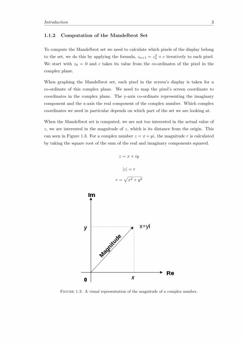
When the Mandelbrot set is computed, we are not too interested in the actual value of

z, we are interested in the magnitude of z, which is its distance from the origin. This

can seen in Figure 1.3. For a complex number z = x+ yi, the magnitude r is calculated

by taking the square root of the sum of the real and imaginary components squared.

z = x+ iy

|z| = r

r =√x2 + y2

Figure 1.3: A visual representation of the magnitude of a complex number.

Introduction 4

If the magnitude of z, for a given pixel on screen, does not exceed 2 after a certain

number of iterations, then it is likely to remain bounded. The pixel belongs to the

Mandelbrot set and is coloured black. If the magnitude of z, for a pixel on screen,

exceeds 2, then it will eventually tend to infinity (Due to the Run Away to Infinity

Criterion. The theorem’s proof can be seen in Appendix A) and the pixel is coloured

based on how many iterations it took for the formula to become unbounded. It should

be noted that each pixel is computed independently of all other pixels.

The behaviour of the magnitude is analogous to squaring a number. Iteratively squaring

a number greater than 1 will cause it to grow forever, however, an iteratively squared

number less than 1 will never grow large, it will get smaller.

1.1.3 Zooming into the Mandelbrot Set

The scale at which we see the Mandelbrot set image is dependent on the size of the

area of the image we are looking at. The zoom level of the image can be adjusted by

adjusting the mapping of the complex plane area to screen area. This ratio is all that

is needed to be changed. The screen area is fixed (as it is a discretely finite array of

pixels), but we can zoom in by specifying that a smaller area of the infinite complex

plane should be mapped to it. Figure 1.4 shows a zoom into an area of the Mandelbrot

set, revealing the characteristic Mandelbrot swirls as well as a smaller copy of the whole

image.

Figure 1.4: A zoom into a section of the Mandelbrot set.

Introduction 5

1.1.4 Computational considerations when Computing the Mandelbrot

Set

1.1.4.1 Finite Resolution

Practically, when computing the Mandelbrot set, we only consider a portion of the

complex plane, the window in which the picture is rendered. A computer monitor’s

display is actually a finite and discrete array of pixels. The complex plane, however, is

continuous and contains an infinite number of points. It is not possible to resolve an

image at a level smaller than a pixel. Due to this, one point in the pixel is taken to

represent a coordinate in the complex plane, usually the centre of the pixel [3]. Figure

1.5, visually demonstrates this.

Figure 1.5: A diagram showing how the centre points of pixels are chosen from afinite pixel array to represent complex numbers [3].

1.1.4.2 Accuracy versus Time

If, for a given pixel, all of z0, . . . , zn lie within a distance of 2 from the origin (have a

magnitude less than 2) for relatively large values of n, we may conclude that the sequence

does not run to infinity. However, this may not be necessarily true. If, for a given pixel,

all of z0 to z1000 lie within a distance of 2 from the origin, but z1001 lies outside we may

incorrectly classify a point as belonging to the Mandelbrot set, when it does not. But

how many iterations are enough? We must make a choice and select some maximum

number of iterations we are willing to try.

As the number of iterations increases, the number of wrong classifications decreases and

the image will have finer detail. Unfortunately, increasing the number of iterations also

increases the computer time needed to generate the picture.

Introduction 6

1.2 FPGA

This section will give a high-level overview of FPGAs, their architecture, how they

function and the hardware device that my implementation is designed for.

FPGAs (Field Programmable Gate Arrays) are programmable digital chips [4]. They

can be thought of as programmable hardware, as they are able to implement an arbitrary

number of digital circuits within the device’s capacity. They are flexible in use and are

designed to be configured by the user after their manufacture.

1.2.1 FPGA Architecture

FPGAs are composed of large numbers of small logic blocks called Logic Cells, which

perform the general logic computations. Logic Cells are typically composed of a 6-input

Lookup table which can act as a small RAM, as can be seen in Figure 1.6. When the

FPGA is configured (the initial programming of the FPGA to set the chosen behaviour

of the logic cells), each logic cell is loaded with the 26 bits holding the Boolean truth

table of the particular logic function we want to implement [5].

Logic cells are grouped to form Logic Clusters which are able compute logic functions of

greater complexity. The Logic clusters are then arranged regularly in the Interconnect

Fabric in an Island-Style architecture [6], as can be seen in Figure 1.7. This enables the

connection of and communication between multiple Logic Clusters.

Figure 1.6: Generic FPGA Logic Element [5].

Along with Logic Clusters, the Island-Style architecture also includes blocks of logic

which implement specific functions efficiently. Block RAM (BRAM) is used for larger

and faster storage while Digital Signal Processing (DSP) Blocks are used for quicker

arithmetic functions such as multiplication. In addition to these, FPGAs also contain

other building blocks such as flip flops and I/O blocks.

Introduction 7

Figure 1.7: Generic Island Style FPGA Architecture [5].

1.2.2 Why use FPGAs ?

The key to the usefulness of an FPGA lies in its ability to be customised. With FPGAs,

the machine can be tailored to needs of the application, giving significant speed ups over

software implemented on CPU or GPUs [7].

In terms of performance, FPGAs excel on stream processing problems as data movement

can be synchronised to minimise data movement on the chip. Furthermore algorithms

can be implemented directly after each other in a chain, eliminating the need for off-chip

communication which provides further performance benefits [8].

Practically, FPGA are used in various domains, from network equipment, to avionics,

to medical devices and data processing [9].

Introduction 8

1.2.2.1 Mandelbrot and FPGAs

We have seen that when computing the Mandelbrot set each pixel is independently iter-

ated on with no data dependencies between pixels. This shows us that the Mandelbrot

Set is an inherently parallelisable and a purely compute-bound problem [10]. It is ideally

suited for computation on FPGAs as an FPGA can take advantage of horizontal scaling

where multiple threads running side by side implement the same algorithm but with

different data [8].

1.2.3 Hardware Platform

For this project I used the Nexys 4 DDR Artix-7 from XILINX [11]. This board, pictured

below, is equipped with 240 DSP slices, 4,860 Kbits of BRAM, 15,850 slices each with

four 6-input LUTs and eight flip-flops.

Figure 1.8: The Xilinx Nexys 4 DDR FPGA Board [11].

Introduction 9

1.3 FPGA Programming

This section will detail the various ways in which an FPGA can be programmed. There

exist several methods to define the behaviour of an FPGA, each with its respective

advantages and disadvantages.

1.3.1 Hardware Description Languages

Hardware Description Languages (HDLs), such as Verilog and VHDL [12], are specialised

text-based computer languages used to describe the structure and behaviour of digital

circuits. They are precise and permit the description of low level details of the hard-

ware relatively directly. HDLs were first created to implement a register-transfer level

abstraction [13] (a model of the data flow and timing of a circuit). Viewed in this way,

HDLs can be compared to the level of abstraction of assembly languages.

Hardware Description Languages are good for smaller circuits, but do not scale well

for larger designs as any high-level components must be detailed at a low level [5, Sec-

tion 2.2.1]. This can make the development process unnecessarily complex.

1.3.2 Schematic Design

Schematic Design makes use of a visualisation of the system, it uses abstract graphical

symbols to represent the system components [14]. While linking boxes with wires on a

screen appears to be much simpler than specifying each component of a system in text,

in practice, it can become more complex. Available schematic editors often have poor

user interfaces. Connecting large numbers of wires and buses on a 2-dimensional page

can quickly become confusing and incomprehensible for larger designs. Furthermore,

schematic design does not permit the programmer to express loop constructs, which are

supported in HDLs.

1.3.3 Hardware Overlays

Hardware Overlays are distinct from HDLs and Schematic Design in that they provide a

layer of abstraction over the FPGA hardware. As mentioned earlier, FPGAs are flexible

and can be programmed to implement any digital circuit within their capacity. In theory

this means that an FPGA can be used to implement another programmable architec-

ture on top of the FPGA fabric, such as an x86 CPU for example. The implemented

Introduction 10

architecture can then be programmed using software alone. Any software that runs on

an actual x86 processor can be directly migrated to the x86 overlay [15], [16].

A major advantage to the hardware overlay approach is that implementing a new or

updated system does not require the use of CAD (Computer Aided Design) tools. This

eliminates the significant amount of time spent on compilation and Place and Route (The

placement and interconnection of logic elements on the FPGA). Furthermore, a system

that has been implemented using an overlay is portable across separate implementations

of the same overlay on different devices [5].

However, there are costs associated with the overlay. Performance suffers, both when

compared to the system implemented directly on the underlying hardware and when

compared to the software running on on a Hard CPU [17].

Introduction 11

1.4 MIPS Architecture

This section will give context about the design of the underlying MIPS system that my

design is to be built on including details the functional design as well as the instruction

set. For this project my system was built upon a base of the MIPS processor overlay

designed by Anders Hauk Fritzell in his Master’s thesis A system for Fast Dynamic

Partial Reconfiguration using GoAhead [18].

MIPS is an acronym for Microprocessor without Interlocked Pipeline Stages. It is a

popular choice in the embedded systems industry, included in devices such as routers

and video game consoles [19]. MIPS is a Reduced Instruction Set Computer (RISC)

architecture. This means that its Instruction Set Architecture (ISA) is made up of

small, fixed-length, heavily optimised instructions that are executable in a single cy-

cle. These instructions are straightforward to decode due to their fixed length format.

Another characteristic trait of MIPS is that memory accesses are exclusively limited to

the load and store instructions and all operations are done within the registers of the

microprocessor [20].

1.4.1 MIPS Functional Blocks

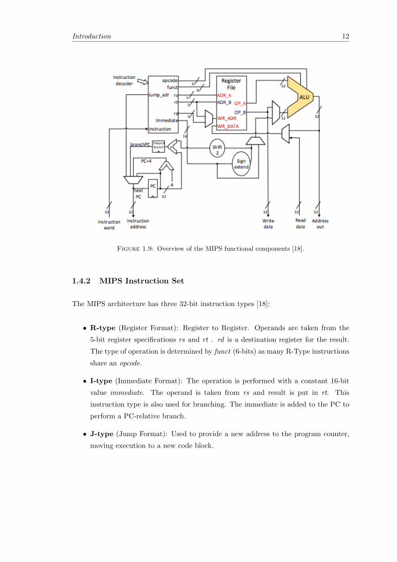
The MIPS processor is composed of several functional blocks as pictured below in Figure

1.9 [18]:

• Instruction Decoder: Takes instructions and decodes them.

• Program Counter (PC): Holds the address of the next instruction to be executed.

• Arithmetic Logic Unit (ALU): A main component that performs the arithmetic

and logical operations on data.

• Registers: 31 general purpose registers , r0 holds a constant zero.

• Memory: Holds the data values to be used. Only accessible through load and

store instructions.

Introduction 12

Figure 1.9: Overview of the MIPS functional components [18].

1.4.2 MIPS Instruction Set

The MIPS architecture has three 32-bit instruction types [18]:

• R-type (Register Format): Register to Register. Operands are taken from the

5-bit register specifications rs and rt . rd is a destination register for the result.

The type of operation is determined by funct (6-bits) as many R-Type instructions

share an opcode.

• I-type (Immediate Format): The operation is performed with a constant 16-bit

value immediate. The operand is taken from rs and result is put in rt. This

instruction type is also used for branching. The immediate is added to the PC to

perform a PC-relative branch.

• J-type (Jump Format): Used to provide a new address to the program counter,

moving execution to a new code block.

Introduction 13

Figure 1.10: MIPS instruction types [18]

In the above table:

• opcode (Operation Code): How an instruction should be decoded.

• rs,rt: Addresses of source register operands.

• rd: Destination register operand.

• shamt (Shift Amount): Used in shift instructions.

• funct: Select the variant of the operation in the opcode field.

• Immediate: 16-bit constant used for constant value operations.

• Address: used in jump instructions to move execution to another part of code.

The MIPS instructions have been designed in this way purposefully. The ISA exhibits

some key underlying principles in the design of hardware.

1. Regularity helps with Simplicity. For example, the two arithmetic instructions add

and subtract both have exactly three operands. This simplifies the design of the

ALU.

2. Smaller is faster, for this reason MIPS only has 32 registers. Having greater num-

bers of registers would lead to an increase in clock cycle time.

3. Make the common case fast. The common case is the case used most frequently.

Increasing the speed of this single option can lead to even greater increases in

overall speed. MIPS addresses this maxim by incorporating constants as part of

the arithmetic instructions and loading small constants into the upper 16-bits of

a register.

Introduction 14

1.5 Number Representations

There are infinitely many real numbers, however a computer is a finite state machine and

thus, can only store a finite amount of information. As numbers cannot be stored with

infinite precision, representing real numbers in a computer always involves an approxi-

mation [21]. This section will explain the 2 main methods of real number representation

on a computer, namely fixed point and floating point.

1.5.1 Floating Point

Floating point numbers are similar in concept to scientific notation. Floating point gains

its name for the fact that the number’s radix point can float. This means that the radix

point can be placed anywhere relative to the a numbers significant digits.

Figure 1.11: How floating point numbers are represented at the bit level [22].

Floating point numbers are composed of two main parts:

• The Mantissa: (or Fraction) Contains the number’s digits.

• The Exponent: Defines where the decimal or binary point is placed relative to

the beginning of the Mantissa. Negative exponents represent numbers less than 1.

1.5.2 Fixed Point

A fixed point number is actually an integer that is scaled by a chosen factor. The

integer values involved in some arithmetic do not represent their normal integer values

but instead represent their values with a radix point at some fixed location. The scaling

factor essentially determines the position of the radix point and is fixed for the duration

of the entire computation.

This concept is most easily understood by examples, in this case with decimal numbers.

If I want to represent the real, fractional value 1.67, I can instead use the value 1670 with

an applied scaling factor of 1/1000. Conversely, the number 252, 000 can be represented

as 252 with a scaling factor of 1000.

Introduction 15

Figure 1.12: How fixed point numbers are represented at the bit level [23]

An example of fixed point arithmetic is the multiplication of 0.0456 ∗ 2.789 = x. First

we multiply both numbers by 10000.

456 ∗ 27890 = y

Now both numbers are integers.

y = 12717840

We have an value for y, but we originally wanted a value for x.

x = y/100002

x = 0.1271784

This is the correct answer computed using only integer arithmetic.

Chapter 2

Design and Implementation

This section will detail the design approach to the project, going into detail on how the

Mandelbrot Set is computed in code. First, an overview of the implemented system will

be given, then the step-by-step details of the implementation process.

2.1 System Implementation Overview

The Mandelbrot set image computation is handled by C code which takes pixel screen

coordinates from an address, computes the colour of the pixel, then returns this colour

to an output address. The C code is then cross compiled into bare-metal instructions.

The bare-metal instructions are then modified to the correct format and placed in the

Instruction ROM of the MIPS overlay. The code is then run on the MIPS CPU overlay

on the FPGA, showing the Mandelbrot Set on screen. This is seen in Figure 2.1.

Figure 2.1: A diagram giving a high-level design overview of the system.

16

Design and Implementation 17

2.2 Mandelbrot C code

The C code can be seen as the starting point of the implementation. The code first takes

pixel screen coordinates from an input address, the inputted pixel coordinates are then

passed to a Mandelbrot computation function. In this function the pixel coordinates on

the screen are mapped to coordinates in the complex plane. The pixel is then iteratively

checked to see if it belongs the Mandelbrot set in a loop. If the pixel does belong to the

set, then the colour black is returned. If not, a colour based on the number of iterations

it took to break out of the loop is returned.

The difficulty in writing the code came from two areas which are discussed below. The

first difficulty came from the fact that complex numbers are not directly represented

in C and the code would need to be implemented using integers. The second difficulty

came from the fact that floating point arithmetic was unsuitable for my implementation

as the MIPS overlay did not have a Floating Point Unit (FPU), so the code needed to

be modified to use fixed point arithmetic.

2.3 Complex Number C code

This section will show how complex number arithmetic can be be computed using a

series of integer calculations [24].

In the Mandelbrot algorithm, we have two complex numbers we make use of : Zn and

c. As mentioned earlier in the Section 1.1.1 of this report, complex numbers are made

up of a real and imaginary part.

As complex numbers have no native type in the C language, we need to find away to

represent them in another way. This can be done using elementary algebra and integers

to represent the imaginary and real components of the complex number.

zn = x+ iy (2.1)

c = a+ ib (2.2)

From the Mandelbrot algorithm we want to compute zn+1 which is the next iteration :

zn+1 = z2n + c

Design and Implementation 18

Below is the expansion of z2n :

z2n = (x+ iy)2 [substituted from (2.1) above]

= x2 + i2xy + i2y2 [expansion of brackets]

= x2 + i2xy − y2 [as i2 = −1 by definition of imaginary numbers

= (x2 − y2) + i2xy [finally, combine the real and imaginary parts]

The end result is also a complex number as it is the addition of real and imaginary

components. To complete the expression, we now add the complex number c to get

zn+1 = z2n + c.

zn+1 = (x2 − y2) + i2xy + c

= (x2 − y2) + i2xy + a+ ib [substituted from (2.2) above]

= (x2 − y2 + a) + i(2xy + b) [combine real and imaginary parts]

Again, we can see the end result is also a complex number, but it has been split into

parts and so can be calculated as a series of integer calculations.

Design and Implementation 19

2.4 Fixed Point Code

This section will contrast fixed and floating point number representations, showing that

for that for this implementation, fixed point is the better choice. Following this, the

implementation details of fixed point will be presented.

2.4.1 Comparison of Fixed and Floating Point Representations for

Mandelbrot

An advantage of floating point is that the floating point exponentiation allows us to

represent numbers with large dynamic ranges (great differences in magnitude). This is

important in cases where the data set is large or the range of the data is unpredictable.

A further advantage of floating point is that most modern programming languages in-

clude a floating point data type, for example the double type in C. Generally speaking,

this makes it simpler to implement a complex algorithm using the floating point type.

Fixed point has no native data type and the code must be modified to accommodate

them.

However there are some drawbacks to floating point. If you know ahead of time that

the numbers you will be using for a given program fall within a small range, then

floating point may not be useful due to the way floating point numbers are represented.

If the numbers are so small that they have a maximum exponent of 1, then the 6-bits

reserved for the exponent are unused and inaccessible. This is the case in the Mandelbrot

computation where all of the numbers used fall with a small range of [-2,2].

Fixed point does not have the disadvantage of wasted bits as the place of the radix point

can be wholly determined by the programmer.

An advantage of fixed point is that implementing an FPGA Overlay which only has

support for fixed point integer arithmetic makes the implemented design substantially

smaller. This has the follow on effect of making the design less expensive in terms of

resources consumed on the FPGA board and also faster.

Another advantage of fixed point is its flexibility of use. The precision, range and data

size can all be chosen by the programmer. This makes fixed point suited to implementa-

tions that require specific data formats. The freedom to choose the precision is crucial

for zooming into the Mandelbrot set image, where at deep zoom levels several hundred

bits of accuracy are needed.

Design and Implementation 20

The major drawback to fixed point is the limited range of representable numbers. The

maximum and minimum fixed point numbers are determined by the maximum and

minimum numbers that can be stored by underlying data type multiplied by the scaling

factor.

It is a common misconception that floating point number representations are generally

preferable for the computation of the Mandelbrot set. While floating point represen-

tations have some advantages, when computing the Mandelbrot set, fixed point is ulti-

mately the winner. As well as this, the MIPS overlay I used in my implementation did

not have a Floating Point Unit (FPU) and so could not support floating point arithmetic.

2.4.2 Scale Factor

In order to gain the extra accuracy gained by use of fixed point number representations,

modifications need to made to the code.

The scale factor determines the position of the radix point, so when the scale factor is

chosen, we are selecting the range and precision of the arithmetic that will be performed

in our program. As we are performing the arithmetic on a binary computer, we choose

a scale factor that is a power of 2 as binary computers are able to quickly multiply and

divide by powers of 2 using logical bit shifting.

For this reason I use the scale of 1/2Shift Factor. I set a constant variable, Shift Factor,

and use it for shifting.

This program uses 32-bit integers, I have chosen a scale factor of 24, meaning that, in

effect, there are 24 decimal places after the radix point and all values will be multiplied

by 224 before their use in any arithmetic.

2.4.2.1 Effect of varying the Scale Factor

A scale factor of 24 has been chosen after experimentation with different scale factors.

As can be seen below in Figures 2.2-4, as the scale factor increases the image quality

of the Mandelbrot Set increases. This is to be expected, as with very few decimal

places available, the coordinates passed to the Mandelbrot computation function are

less accurate.

The first image, with a scale factor of 4, is of poor quality and is pixelated, although it

still retains the characteristic Mandelbrot set shape. When the scale factor is increased to

8, there is an significant jump in image quality. When further increased, the improvement

Design and Implementation 21

in image quality is much less noticeable at this scale, but upon zooming in finer detail

than the previous images is visible.

All these images were computed by the Mandelbrot test program using a constant res-

olution of 2560 x 1440.

Figure 2.2: Mandelbrot render with scale factor 4.

Figure 2.3: Mandelbrot render with scale factor 8.

Figure 2.4: Mandelbrot render with scale factor 24.

.

Design and Implementation 22

2.4.3 Conversion

This subsection shows how different functions are used to convert between fixed point

integer representations and normal integers.

Figure 2.5: Macros for handling fixed point numbers.

Above we can see the macro functions that are used for fixed point arithmetic.

MultiplyFixed(): takes two large integers as input and multiplies them together. The

product is then rescaled by right-shifting it by the shift amount.

FixedPointConvert(): takes a Fixed Point integer value as input, converts it to a long

integer and multiplies it by 1 shifted by the scale factor to produce the output. This is

equivalent to multiplying the number by 2Shift Amount.

integer(): takes a long integer value and converts it into a small fixed point number

by adding it to 2Shift Amount−1, then rescaling the sum by right-shifting by the shift

amount.

Figure 2.6: Unmodified main loop body of Mandelbrot computation using floatingpoint numbers.

Figure 2.7: Modified main loop body of Mandelbrot computation using fixed pointnumbers.

In Figures 2.6 and 2.7 we see the comparison of the original floating point implementa-

tion and the fixed point implementation of the main loop of the Mandelbrot computa-

tion. The different implementations are almost identical in structure, but in the fixed

point implementation most arithmetic performed on the values is handled by the macro

functions defined in Figure 2.5.

Design and Implementation 23

As can be seen in Figure 2.7, the defined macros can then be simply substituted into the

code to make it fixed point. An advantage of this approach is that the same fixed point

macros can be used to convert other programs to fixed point with little additional work.

As previously stated, the MIPS overlay used in this design does not include a Floating

Point Unit, so this feature is necessary when expanding the design to compute an image

other than the Mandelbrot set.

2.5 Cross Compilation

This section will cover one of the central elements of this systems design, the method

by which the C code is able to run on the overlay. It will give a brief overview of

compilers, then provide some detail on the implementation of the cross compiler used in

this project.

A compiler is a program that generates executable code from source code. Typically,

what is colloquially referred to as a compiler is actually a native compiler. A native

compiler runs on a specific type of computer and generates code to also run on that

same specific type of computer.

A cross compiler is a compiler that runs on one platform (called the host) but gener-

ates executable code for another, different platform (called the target) [25]. The two

platforms may have different operating systems and even different CPUs. An easily

understood example would be a Microsoft Windows compiler generating code for Apple

iOS device.

Cross compilation has several applicable uses, such as embedded systems design. The

embedded device is unlikely to have the computing resources to run a development

environment or a compiler. Another example is Bootstrapping, a process in which a

compiler is written in the source programming language which it intends to compile.

2.5.1 Building the Cross Compiler Toolchain

For this project I needed a compiler which would take C code and output a bare metal

executable. I had a choice of two cross compilers, the mips-linux-gnu and the mipsel-elf.

Both of these compilers met the above requirement, the decision came down to using

both compilers to compile a short test program, then using objdump(A program that

displays information about object files) to view the assembly code and comparing which

came closer to my desired output. I chose the ’mips-linux-gnu’ cross compiler as the

compiler’s target platform is bare-metal MIPS, its host platform is a linux machine.

Design and Implementation 24

2.6 Effects of Number of Iterations on Image Quality

This section shows some of the experimentation that was carried out in order to deter-

mine the optimum number of iterations to set for the final implementation.

As mentioned in Section 1.1.4.2, there is a trade off between the accuracy of the image

and the time spent computing the image. A choice needs to be made on the number of

iterations before it is decided that a pixel does or does not belong to the Mandelbrot

set. Before running the simulation, I experimented with what the minimum number of

iterations was to see acceptable levels of detail.

The main factor in this case is image quality, as there is nothing gained by fast compu-

tation if the image is of poor quality.

Below we can see the Mandelbrot images that is computed using different maximum

numbers of iterations. The colour yellow indicates the points that the Mandelbrot

computation has decided belong to the Mandelbrot set.

In Figure 2.8a, when the maximum number of iterations is limited to 128, the image

quality is extremely poor and ”blob-like”. There is almost no fine detail visible and

bands of colour can be clearly seen. The large yellow region shows that at such a low

number of iterations there have been many wrong classifications. However, even at this

low number the overall outline is still correct.

When the maximum number of iterations doubles to 256 in Figure 2.8b, some fine detail

is now visible but the bands of colour can still be seen and the centre regions still appear

blob-like.

Figure 2.8c makes a jump in the maximum number of iterations to 896. It is very

detailed and clear. No bands of colour can be seen and the image resembles particles

rather than blobs.

Past 896, an increase in the maximum number of iterations has little effect. In Figure

2.8d the maximum number of iterations is set at 3768. This is a significant jump up

from 896 but the images are almost identical.

For my implementation I chose a final maximum number of iterations of 896 as beyond

this point there is no image improvement to be gained but the time to compute the

image increases.

Design and Implementation 25

(a) Max Iterations: 128 (b) Max Iterations: 256

(c) Max Iterations: 896 (d) Max Iterations: 3768

Figure 2.8: A magnified section of the Mandelbrot set image computed using anincreasing number of maximum of iterations.

Chapter 3

Evaluation

This section gives an overview of ensuring the correctness of the output of the imple-

mentation.

3.1 Code Evaluation

In order to evaluate the correctness of the C code, I ran the main body of the code in

modified evaluation program. This program functions by taking the screen co-ordinates

from a memory address in the same way as if was the code was running on an FPGA, but

rather than outputting the results to memory, the output is placed in a Portable Pixmap

Format (PPM). PPM was chosen as it is an image file format ideal for use in Mandelbrot

as images are stored as an array of pixel colour values. Mandelbrot correctness is best

confirmed visually, if the code is even slightly wrong, the output will be far from similar

to the correct image.

26

Evaluation 27

3.2 Simulation

The purpose of simulation is to verify the functionality and timing of a design by in-

terpreting VHDL code as if it was circuit functionality. The logical results are then

displayed on screen [26]. For the simulation I used XILINX’s ISE Simulator, ISIM. Sim-

ulation makes use of a Test Bench, which is HDL code that provides a set of stimuli to

the simulation[27].

To start, compiled and formatted instructions are inserted into the MIPS Instruction

BRAM. This is seen in Figure 3.5, the comments beside the instructions show their

meaning in assembly.

Figure 3.1: A screen shot of the some of the cross-compiled assembly code in the theInstruction BRAM of the MIPS overlay.

After this ISIM is launched. In Figure 3.6 we see the button in ISE whcih launches

ISIM. Before ISIM is launched, ISE performs a check of the behavioural syntax of the

source file [28].

Figure 3.2: A screen shot showing the button which launches the simulator afterchecking the Behavioural Syntax.

Evaluation 28

Figure 3.7 shows the behavioural simulation running. In this image the scale is per

microsecond. Verification is possible by taking note of the most important signals as seen

in Figure 3.8. By manually checking what I expect the address of the next instruction

to be, I can ensure that the design is functionally working and correct.

Figure 3.3: A screen shot of the simulation window.

Figure 3.4: A close up screen shot of the most relevant signals in the simulation.

Chapter 4

Reflections and Conclusion

4.1 Change of Objective

Initially, this project’s objective was to render the Mandelbrot set on a dedicated FPGA

Processing Element, rather than use a MIPS hardware overlay. After a few weeks of

preliminary research, and after a discussion with my project supervisor, it was decided

that the current project objective was a more worthwhile third year project. The mod-

ified project would be more applicable to hardware design in the real world, it would

allow me to learn about a wider variety of topic areas and it would be flexible enough

to be expanded upon (See chapter 5).

4.2 Challenges

Over the course of this project I faced a few roadblocks to my progress. While I had

budgeted time for unexpected events, overcoming the hurdles took longer than expected.

This had the unfortunate effect of slowing down all progress, as I could not continue

with the later stages.

On university machines, undergraduate students are not able to gain superuser access

for administrator privileges. As I was unable to gain admin privileges, I was unable to

correctly compile the cross compiler toolchain. This was a crucial step as it allows both

parts of the system (C code and MIPS overlay) to work together.

This was overcome by the use of an Oracle VirtualBox Virtual Machine [29] running

from a 32GB Flash Drive. On this virtual machine I then installed a 64-bit Ubuntu

version 14.04.4 (Long Term Support version). This granted me full admin privileges and

I did all of my cross compilation on this virtual machine.

29

Reflections and Conclusion 30

4.3 Conclusion

I was motivated to choose the project as I had held an interest in fractal images and

their appearance in nature for a long time. I also saw the project as an opportunity to

learn more about the topic area of hardware, as coming into the project, I had almost

no computer hardware programming knowledge, let alone FPGA knowledge.

As could be expected, the learning curve for this project was relatively steep for me

as hardware design differs significantly from software design. Furthermore, as FPGAs

are not widely used consumer products, the information and resources available on

this topic are rarely written for the audience of a newcomer to FPGA programming.

Nonetheless I took this as a challenge and taught myself the basics of both popular

hardware description languages, VHDL and Verilog to understand the existing code

base.

Overall, I would describe this project as beneficial and worthwhile. Although I did not

implement as much as I would have ideally liked to, I have enjoyed the process and I

have learnt a great amount through research. I have tried to express this in this report.

Along with the technical knowledge gained in the implementation of a large project, I

have also learnt equally valuable soft-skills such as organisation, time boxing and most

importantly how to enthuse others about your ideas.

Chapter 5

Further Research

5.1 The Mandelbulb

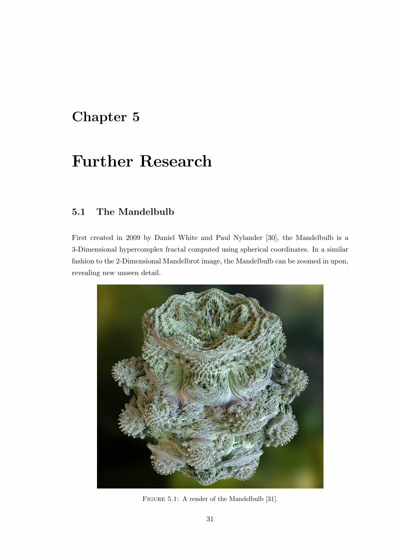
First created in 2009 by Daniel White and Paul Nylander [30], the Mandelbulb is a

3-Dimensional hypercomplex fractal computed using spherical coordinates. In a similar

fashion to the 2-Dimensional Mandelbrot image, the Mandelbulb can be zoomed in upon,

revealing new unseen detail.

Figure 5.1: A render of the Mandelbulb [31].

31

Further Research 32

5.1.1 Changes to be Made

In order to render the Mandelbulb on the current FPGA system, some changes would

need to be made as the computation of the Mandelbulb differs from the Mandelbrot set

in that it is 3-dimensional.

The Mandelbulb C code computes whether a given point in 3D space belongs to the

Mandelbulb. By doing this a surface of the Mandelbulb is constructed. However,This

is not enough to display the image on a screen. To display the image, we would need

to use a Ray-marching, a simplistic 3D rendering technique which allows one to create

an image of a surface by only knowing the distance from the surface to any point. Ray-

marching would require some additional code to implement, but most of the structure

of the system has been implemented.

Appendix A

Run Away to Infinity Criterion

Here I will show that if some zn is farther than 2 from the origin, then successive iterates

will grow without bound. That is, they will run away to ∞ [32].

For a complex number zn = xn + iyn , the absolute value is

|zn| =√

(x2n + y2n),

the distance from zn to the origin.

Recalling the sequence z0, z1, . . . is defined by zn+1 = z2n + c, we show if some zn satisfies

|zn| > max(2, |c|), then the sequence zn, zn+1, . . . runs away to ∞. So suppose |zn| >max(2, |c|).

Because |zn| > 2 , we can write

|zn| = 2 + ε,

for some ε > 0.

Now

|z2n| = |z2n + c− c| ≤ |z2n + c|+ |c|

So

|z2n + c| ≥ |z2n| − |c| = |zn|2 − |c|

> |zn|2 − |zn|(because|zn| > |c|)

= (|zn| − 1) · |zn| = (1 + ) · |zn|

That is, |zn+1| > (1 + ) · |zn|. Iterating, |zn+k| > (1 + )k · |zn|.

33

Further Research 34

To complete the proof that |zn| > 2 implies the sequence runs away to infinity, observe

that if |c| > 2, then

z0 = 0

z1 = c

andz2 = c2 + c = c · (c+ 1)

so|z2| = |c| · |c+ 1| > |c|(noting|c+ 1| > 1because|c| > 2).

Bibliography

[1] John Hutchinson. Fractals and Self-Similarity. Indiana University Mathematics

Journal, 30(5):713–747, 1981.

[2] Nigel Lesmoir-Gordon. The Colours of Infinity: The Beauty, The Power and the

Sense of Fractals. Clear Books, 2004. ISBN 1904555055.

[3] Michael Frame and Nial Neger. Julia sets - computational issues. URL http:

//users.math.yale.edu/public_html/People/frame/Fractals/. [Accessed :

20/03/2016].

[4] Frank Hannig Dirk Koch, Daniel Ziener. FPGAs For Software Programmers.

Springer, 2016.

[5] Charles Eric LaForest. High-Speed Soft-Processor Architecture for FPGA Overlays.

PhD thesis, University of Toronto, 2015.

[6] Ian Kuon, Russell Tessier, and Jonathan Rose. Fpga architecture: Survey and

challenges. Foundations and Trends in Electronic Design Automation, 2(2):46, 2008.

ISSN 1551-3939. doi: 10.1561/1000000005. URL http://dx.doi.org/10.1561/

1000000005.

[7] Wim Vanderbauwhede. High-performance computing using FPGAs. Springer, New

York, NY, 2013. ISBN 978-1-4614-1790-3.

[8] D. Koch, F. Hannig, and D. Ziener. FPGAs for Software Programmers. Springer

International Publishing, 2016. ISBN 9783319264066.

[9] Field programmable gate array. URL http://www.xilinx.com/training/fpga/

fpga-field-programmable-gate-array.htm. [Accessed : 5/03/2016].

[10] J. Kepner. Parallel MATLAB for Multicore and Multinode Computers. SIAM e-

books. Society for Industrial and Applied Mathematics (SIAM, 3600 Market Street,

Floor 6, Philadelphia, PA 19104), 2009. ISBN 9780898718126.

[11] Nexys4 ddr artix-7 fpga board. URL http://www.xilinx.com/products/

boards-and-kits/1-6olhwl.html. [Accessed : 13/04/2016].

35

Bibliography 36

[12] H. Tucker Jerry. Hardware description languages.

[13] M.D. Ciletti. Advanced Digital Design with the Verilog HDL. Pearson Educa-

tion, 2011. ISBN 9780133002546. URL https://books.google.co.uk/books?id=

QTArAAAAQBAJ.

[14] F. Rodriguez-Henriquez, N.A. Saqib, A.D. Perez, and C.K. Koc. Cryptographic

Algorithms on Reconfigurable Hardware. Signals and Communication Technology.

Springer US, 2007. ISBN 9780387366821.

[15] Graham Schelle, Jamison Collins, Ethan Schuchman, Perrry Wang, Xiang Zou,

Gautham Chinya, Ralf Plate, Thorsten Mattner, Franz Olbrich, Per Hammar-

lund, Ronak Singhal, Jim Brayton, Sebastian Steibl, and Hong Wang. Intel ne-

halem processor core made fpga synthesizable. In Proceedings of the 18th An-

nual ACM/SIGDA International Symposium on Field Programmable Gate Arrays,

FPGA ’10, pages 3–12, New York, NY, USA, 2010. ACM. ISBN 978-1-60558-911-4.

[16] Perry H. Wang, Jamison D. Collins, Christopher T. Weaver, Blliappa Kuttanna,

Shahram Salamian, Gautham N. Chinya, Ethan Schuchman, Oliver Schilling,

Thorsten Doil, Sebastian Steibl, and Hong Wang. Intel R©atomTMprocessor core

made fpga-synthesizable. In Proceedings of the ACM/SIGDA International Sympo-

sium on Field Programmable Gate Arrays, FPGA ’09, pages 209–218, New York,

NY, USA, 2009. ACM. ISBN 978-1-60558-410-2.

[17] A. Koch, R. Krishnamurthy, J. McAllister, R. Woods, and T. El-Ghazawi. Recon-

figurable Computing: Architectures, Tools and Applications: 7th International Sym-

posium, ARC 2011, Belfast, UK, March 23-25, 2011, Proceedings. Lecture Notes

in Computer Science. Springer Berlin Heidelberg, 2011. ISBN 9783642194757.

[18] Anders Hauk Fritzell. A system for fast dynamic partial reconfiguration using

goahead: Design and implementation. pages 28,37, 2013.

[19] D. Sweetman. See MIPS Run. The Morgan Kaufmann Series in Computer Archi-

tecture and Design. Elsevier Science, 2010. ISBN 9780080525235.

[20] J.L. Hennessy and D.A. Patterson. Computer Architecture: A Quantitative Ap-

proach. The Morgan Kaufmann Series in Computer Architecture and Design. Else-

vier Science, 2006. ISBN 9780080475028.

[21] David Goldberg. What every computer scientist should know about floating-point

arithmetic. ACM Comput. Surv., 23(1):5–48, March 1991. ISSN 0360-0300.

[22] Ieee 754 single floating point format. URL https://commons.wikimedia.

org/wiki/File:IEEE_754_Single_Floating_Point_Format.svg. [Accessed :

7/02/2016].

Bibliography 37

[23] Fixed point arithmetic. URL http://radio.feld.cvut.cz/matlab/toolbox/

filterdesign/quant14a.html. [Accessed : 6/02/2016].

[24] Brain Hall. The mandelbrot set. URL http://beej.us/blog/data/

mandelbrot-set/. [Accessed : 25/04/2016].

[25] Why do i need a cross compiler ? URL http://wiki.osdev.org/Why_do_I_need_

a_Cross_Compiler%3F. [Accessed : 28/04/2016].

[26] Simulation overview. . URL http://www.xilinx.com/itp/xilinx10/isehelp/

ise_c_simulation_overview.htm. [Accessed : 27/04/2016].

[27] Test benches. . URL http://www.xilinx.com/itp/xilinx10/isehelp/ise_c_

simulation_test_bench.htm. [Accessed : 27/04/2016].

[28] Checking syntax for simulation. . URL http://www.xilinx.com/itp/xilinx10/

isehelp/pp_p_process_check_syntax_simulation.htm.

[29] Virtualbox manual. URL https://www.virtualbox.org/manual/ch01.html. [Ac-

cessed : 28/04/2016].

[30] Paul Nylander. Hypercomplex fractals. URL http://bugman123.com/

Hypercomplex/. [Accessed : 20/04/2016].

[31] Ondrej Karlik. Power 8 mandelbulb fractal overview. URL https://en.

wikipedia.org/wiki/File:Power_8_mandelbulb_fractal_overview.jpg. [Ac-

cessed : 27/04/2016].

[32] Michael Frame. Run away to infinity criterion. URL http://users.math.yale.

edu/public_html/People/frame/Fractals/. [Accessed : 5/03/2016].