arX

iv:1

305.

5777

v4 [

cs.C

V]

3 S

ep 2

014

MANUSCRIPT OF IEEE TRANSACTIONS ON IMAGE PROCESSING, EDICS: SMR-REP 1

Compressive Sensing of Sparse TensorsShmuel Friedland, Qun Li*,Member, IEEE, and Dan Schonfeld,Fellow, IEEE

Abstract—Compressive sensing (CS) has triggered enormousresearch activity since its first appearance. CS exploits the signal’ssparsity or compressibility in a particular domain and integratesdata compression and acquisition, thus allowing exact reconstruc-tion through relatively few non-adaptive linear measurements.While conventional CS theory relies on data representationin theform of vectors, many data types in various applications such ascolor imaging, video sequences, and multi-sensor networks, areintrinsically represented by higher-order tensors. Application ofCS to higher-order data representation is typically performedby conversion of the data to very long vectors that must bemeasured using very large sampling matrices, thus imposinga huge computational and memory burden. In this paper,we propose Generalized Tensor Compressive Sensing (GTCS)–a unified framework for compressive sensing of higher-ordertensors which preserves the intrinsic structure of tensor datawith reduced computational complexity at reconstruction.GTCSoffers an efficient means for representation of multidimensionaldata by providing simultaneous acquisition and compression fromall tensor modes. In addition, we propound two reconstructionprocedures, a serial method (GTCS-S) and a parallelizablemethod (GTCS-P). We then compare the performance of theproposed method with Kronecker compressive sensing (KCS) andmulti-way compressive sensing (MWCS). We demonstrate exper-imentally that GTCS outperforms KCS and MWCS in termsof both reconstruction accuracy (within a range of compressionratios) and processing speed. The major disadvantage of ourmethods (and of MWCS as well), is that the compression ratiosmay be worse than that offered by KCS.

Index Terms—Compressive sensing, compression ratio, convexoptimization, multilinear algebra, higher-order tensor, general-ized tensor compressive sensing.

I. I NTRODUCTION

Recent literature has witnessed an explosion of interest insensing that exploits structured prior knowledge in the generalform of sparsity, meaning that signals can be represented byonly a few coefficients in some domain. Central to much ofthis recent work is the paradigm of compressive sensing (CS),also known under the terminology of compressed sensingor compressive sampling [?], [?], [?]. CS theory permitsrelatively few linear measurements of the signal while stillallowing exact reconstruction via nonlinear recovery process.The key idea is that the sparsity helps in isolating the orig-inal vector. The first intuitive approach to a reconstruction

Copyright (c) 2013 IEEE. Personal use of this material is permitted.However, permission to use this material for any other purposes must beobtained from the IEEE by sending a request to pubs-permissions@ieee.org.

S. Friedland is with the Department of Mathematics, Statistics & ComputerScience, University of Illinois at Chicago (UIC), Chicago,IL, 60607-7045USA. e-mail: friedlan@uic.edu. This work was supported by NSF grant DMS-1216393.

Q. Li is with PARC, Xerox Corporation, Webster, NY, 14580 USA. e-mail: Qun.Li@xerox.com. This work was done during her PhD study at UIC,advised by Prof. Schonfeld.

D. Schonfeld is with the Department of Electrical and Computer Engi-neering, University of Illinois at Chicago, Chicago, IL, 60607 USA. e-mail:dans@uic.edu.

algorithm consists in searching for the sparsest vector thatis consistent with the linear measurements. However, thisℓ0-minimization problem is NP-hard in general and thus compu-tationally infeasible. There are essentially two approaches fortractable alternative algorithms. The first is convex relaxation,leading toℓ1-minimization [?], also known as basis pursuit[?], whereas the second constructs greedy algorithms. Besides,in image processing, the use of total-variation minimizationwhich is closely connected toℓ1-minimization first appears in[?] and is widely applied later on. By now basic propertiesof the measurement matrix which ensure sparse recovery byℓ1-minimization are known: the null space property (NSP) [?]and the restricted isometry property (RIP) [?].

An intrinsic limitation in conventional CS theory is thatit relies on data representation in the form of vectors. Infact, many data types do not lend themselves to vector datarepresentation. For example, images are intrinsically matrices.As a result, great efforts have been made to extend traditionalCS to CS of data in matrix representation. A straightforwardimplementation of CS on 2D images recasts the 2D problemas traditional 1D CS problem by converting images to longvectors, such as in [?]. However, despite of considerablyhuge memory and computational burden imposed by the useof long vector data and large sampling matrix, the sparsesolutions produced by straightforwardℓ1-minimization oftenincur visually unpleasant, high-frequency oscillations.This isdue to the neglect of attributes known to be widely possessedby images, such as smoothness. In [?], instead of seekingsparsity in the transformed domain, a total variation-basedminimization was proposed to promote smoothness of thereconstructed image. Later, as an alternative for alleviating thehuge computational and memory burden associated with imagevectorization, block-based CS (BCS) was proposed in [?]. InBCS, an image is divided into non-overlapping blocks andacquired using an appropriately-sized measurement matrix.

Another direction in the extension of CS to matrix CS gen-eralizes CS concept and outlines a dictionary relating conceptsfrom cardinality minimization to those of rank minimization[?], [?], [?]. The affine rank minimization problem consistsof finding a matrix of minimum rank that satisfies a given setof linear equality constraints. It encompasses commonly seenlow-rank matrix completion problem [?] and low-rank matrixapproximation problem as special cases. [?] first introducedrecovery of the minimum-rank matrix via nuclear norm min-imization. [?] generalized the RIP in [?] to matrix case andestablished the theoretical condition under which the nuclearnorm heuristic can be guaranteed to produce the minimum-rank solution.

Real-world signals of practical interest such as color imag-ing, video sequences and multi-sensor networks, are usuallygenerated by the interaction of multiple factors or multi-

media and thus can be intrinsically represented by higher-order tensors. Therefore, the higher-order extension of CStheory for multidimensional data has become an emergingtopic. One direction attempts to find the best rank-R tensorapproximation as a recovery of the original data tensor asin [?], they also proved the existence and uniqueness ofthe best rank-R tensor approximation in the case of 3rdorder tensors under appropriate assumptions. In [?], multi-way compressed sensing (MWCS) for sparse and low-ranktensors suggests a two-step recovery process: fitting a low-rank model in compressed domain, followed by per-modedecompression. However, the performance of MWCS relieshighly on the estimation of the tensor rank, which is an NP-hard problem. The other direction [?] [?] uses Kroneckerproduct matrices in CS to act as sparsifying bases that jointlymodel the structure present in all of the signal dimensionsas well as to represent the measurement protocols used indistributed settings. However, the recovery procedure, due tothe vectorization of multidimensional signals, is rather timeconsuming and not applicable in practice. We proposed in [?]Generalized Tensor Compressive Sensing (GTCS)–a unifiedframework for compressive sensing of higher-order tensors. Inaddition, we presented two reconstruction procedures, a serialmethod (GTCS-S) and a parallelizable method (GTCS-P). Ex-perimental results demonstrated the outstanding performanceof GTCS in terms of both recovery accuracy and speed. In thispaper, we not only illustrate the technical details of GTCSmore thoroughly, but also further examine its performanceon the recovery of various types of data including sparseimage, compressible image, sparse video and compressiblevideo comprehensively.

The rest of the paper is organized as follows. SectionII briefly reviews concepts and operations from multilinearalgebra used later in the paper. It also introduces conven-tional compressive sensing theory. Section III proposes GTCStheorems along with their detailed proofs. Section IV thencompares experimentally the performance of the proposedmethod with existing methods. Finally, Section V concludesthe paper.

II. BACKGROUND

Throughout the discussion, lower-case characters representscalar values(a, b, . . .), bold-face characters represent vectors(a,b, . . .), capitals represent matrices(A,B, . . .) and calli-graphic capitals represent tensors(A,B, . . .). Let [N ] denotethe set{1, 2, . . . , N}, whereN is a positive integer.A. Multilinear algebra

A tensor is a multidimensional array. The order of a tensoris the number of modes. For instance, tensorX ∈ R

N1×...×Nd

has orderd and the dimension of itsith mode (also calledmodei directly) isNi.

Kronecker product The Kronecker product of matricesA ∈R

I×J andB ∈ RK×L is denoted byA ⊗ B. The result is a

matrix of size(I ·K)× (J · L) defined by

A⊗B =

a11B a12B · · · a1JB

a21B a22B · · · a2JB...

.... . .

...aI1B aI2B · · · aIJB

.

Outer product and tensor product The operator◦ denotesthe tensor product between two vectors. In linear algebra, theouter product typically refers to the tensor product betweentwo vectors, that is,u◦v = uv⊤. In this paper, the terms outerproduct and tensor product are equivalent. The Kroneckerproduct and the tensor product between two vectors are relatedby u ◦ v = u⊗ v⊤.

Mode-i product The mode-i product of a tensorX =[xα1,...,αi,...,αd

] ∈ RN1×...×Ni×...×Nd and a matrixU =

[uj,αi] ∈ R

J×Ni is denoted byX ×i U and is of sizeN1×. . .×Ni−1×J×Ni+1×. . .×Nd. Element-wise, the mode-i product can be written as(X ×i U)α1,...,αi−1,j,αi+1,...,αd

=∑Ni

αi=1 xα1,...,αi,...,αduj,αi

.

Mode-i fiber and mode-i unfolding A mode-i fiber of a ten-sorX = [xα1,...,αi,...,αd

] ∈ RN1×...×Ni×...×Nd is obtained by

fixing every index butαi. The mode-i unfoldingX(i) of Xarranges the mode-i fibers to be the columns of the resultingNi × (N1 · . . . ·Ni−1 ·Ni+1 · . . . ·Nd) matrix.Y = X×1U1×. . .×dUd is equivalent toY(i) = UiX(i)(Ud⊗

. . .⊗ Ui+1 ⊗ Ui−1 ⊗ . . .⊗ U1)⊤.

Core Tucker decomposition [?] Let X ∈ RN1×...×Nd with

mode-i unfoldingX(i) ∈ RNi×(N1·...·Ni−1·Ni+1·...·Nd). Denote

by Ri(X ) ⊂ RNi the column space ofX(i) whose rank is

ri. Let c1,i, . . . , cri,i be a basis inRi(X ). Then the subspaceV(X ) := R1(X ) ◦ . . . ◦ Rd(X ) ⊂ R

N1×...×Nd containsX .Clearly a basis inV consists of the vectorsci1,1 ◦ . . . ◦ cid,dwhere ij ∈ [rj ] and j ∈ [d]. Hence the core Tuckerdecomposition ofX is

X =∑

ij∈[rj ],j∈[d]

ξi1,...,idci1,1 ◦ . . . ◦ cid,d. (1)

A special case of core Tucker decomposition is the higher-order singular value decomposition (HOSVD). Any tensorX ∈ R

N1×...×Nd can be written as

X = S ×1 U1 × . . .×d Ud, (2)

whereUi = [u1 · · ·uNi] is orthogonal fori ∈ [d] and S is

called the core tensor which can be obtained easily byS =X ×1 U

⊤1 × . . .×d U

⊤d .

There are many ways to get a weaker decomposition as

X =

K∑

i=1

a(1)i ◦ . . . ◦ a(d)i , a

(j)i ∈ Rj(X ), j ∈ [d]. (3)

A simple constructive way is as follows. First decomposeX(1)

asX(1) =∑r1

j=1 cj,1g⊤j,1 (e.g. by singular value decomposi-

tion (SVD)). Now eachgj,1 can be represented as a tensor oforder d − 1 ∈ R2(X ) ◦ . . . ◦ Rd(X ) ⊂ R

N2×...×Nd . Unfoldeachgj,1 in mode2 to obtaingj,1(2) and decomposegj,1(2) =∑r2

l=1 dl,2,jf⊤l,2,j , dl,2,j ∈ R2(X ), fl,2,j ∈ R3(X ) ◦ . . . ◦

Rd(X ). By successively unfolding and decomposing eachremaining tensor mode, a decomposition of the form in Eq. (3)is obtained. Note that ifX is s-sparse then each vector inRi(X ) is s-sparse andri ≤ s for i ∈ [d]. HenceK ≤ sd−1.

CANDECOMP/PARAFAC decomposition [?] For a tensorX ∈ R

N1×...×Nd , the CANDECOMP/PARAFAC (CP) decom-position isX ≈ [λ;A(1), . . . , A(d)] ≡

∑Rr=1 λra

(1)r ◦ . . .◦a(d)r ,

whereλ = [λ1 . . . λR]⊤ ∈ R

R and A(i) = [a(i)1 · · · a(i)R ] ∈

RNi×R for i ∈ [d].

B. Compressive sensing

Compressive sensing is a framework for reconstruction ofsignals that have sparse representations. A vectorx ∈ R

N

is called s-sparse if it has at mosts nonzero entries. TheCS measurement protocol measures the signalx with themeasurement matrixA ∈ R

m×N wherem < N and encodesthe information asy ∈ R

m where y = Ax. The decoderknowsA and attempts to recoverx from y. Sincem < N ,typically there are infinitely many solutions for such an under-constrained problem. However, ifx is known to be sufficientlysparse, then exact recovery ofx is possible, which establishesthe fundamental tenet of CS theory. The recovery is achievedby finding a solutionz⋆ ∈ R

N satisfying

z⋆ = argmin{‖z‖1, Az = y}. (4)

Such z⋆ coincides withx under certain condition. The fol-lowing well known result states that eachs-sparse signal canbe recovered uniquely ifA satisfies the null space property oforders, denoted as NSPs. That is, ifAw = 0,w ∈ R

N \{0},then for any subsetS ⊂ {1, 2, . . . , N} with cardinality|S| = s

it holds that‖vS‖1 < ‖vSc‖1, wherevS denotes the vectorthat coincides withv on the index setS and is set to zero onSc.

One way to generate suchA is by sampling its entries usingnumbers generated from a Gaussian or a Bernoulli distribution.This matrix generation process guarantees that there exists auniversal constantc such that if

m ≥ 2cs lnN

s, (5)

then the recovery ofx using (4) is successful with probabilitygreater than1− exp(−m

2c ) [?].In fact, most signals of practical interest are not really sparse

in any domain. Instead, they are only compressible, meaningthat in some particular domain, the coefficients, when sortedby magnitude, decay according to the power law [?]. Given asignalx ∈ R

N which can be represented byθ ∈ RN in some

transformed domain, i.e.x = Φθ, with sorted coefficients suchthat ‖θ‖(1) ≥ . . . ≥ ‖θ‖(N), it obeys that‖θ‖(n) ≤ Rn− 1

p foreachn ∈ [N ], where0 < p < 1 and R is some constant.According to [?], [?], when A is drawn randomly from aGaussian or Bernoulli distribution andΦ is an orthobasis, withoverwhelming probability, the solutiong⋆ ∈ R

N to

g⋆ = argmin{‖g‖1, AΦg = y} (6)

is unique. Furthermore, denote byx♯ the recovered signalvia x♯ = Φg, with a very large probability we have theapproximation

‖x− x♯‖2 ≤ CR(m

lnN)

12− 1

p ,

whereA ∈ Rm×N is generated randomly as stated above,

m is the number of measurements, andC is some constant.This provides theoretical foundation for CS of compressiblesignals.

Consider the case where the observationy is noisy. For agiven integers, a matrixA ∈ R

m×N satisfies the restrictedisometry property (RIPs) if

(1− δs)‖x‖2 ≤ ‖Ax‖2 ≤ (1 + δs)‖x‖2for all s-sparsex ∈ R

N and for someδs ∈ (0, 1). Given anoisy observationy with bounded errorǫ, an approximationof the signalx, f⋆ ∈ R

N , can be obtained by solving thefollowing relaxed recovery problem [?],

f⋆ = argmin{‖f‖1, ‖Af − y‖2 ≤ ǫ}. (7)

It is known that ifA satisfies the RIP2s property withδ2s ∈(0,

√2− 1), then

‖f⋆ − x‖2 ≤ C2ǫ, whereC2 =4√1 + δ2s

1− (1 +√2)δ2s

. (8)

Recently, the extension of CS theory for multidimensionalsignals has become an emerging topic. The objective of ourpaper is to consider the case where thes-sparse vectorxis represented as ans-sparse tensorX = [xi1,i2,...,id ] ∈R

N1×N2×...×Nd . Specifically, in the sampling phase, we con-struct a set of measurement matrices{U1, U2, . . . , Ud} for alltensor modes, whereUi ∈ R

mi×Ni for i ∈ [d], and sampleXto obtainY = X ×1U1×2U2× . . .×dUd ∈ R

m1×m2×...×md .Note that our sampling method is mathematically equivalentto that proposed in [?], whereA is expressed as a KroneckerproductA := U1⊗U2⊗ . . .⊗Ud, which requiresm to satisfy

m ≥ 2cs(− ln s+d

∑

i=1

lnNi). (9)

We show that if eachUi satisfies the NSPs property, thenwe can recoverX uniquely fromY by solving a sequenceof ℓ1 minimization problems, each similar to the expressionin (4). This approach is advantageous relative to vectorization-based compressive sensing methods because the correspondingrecovery problems are in terms ofUi’s instead ofA, whichresults in greatly reduced complexity. If the entries ofUi

are sampled from Gaussian or Bernoulli distributions, thefollowing set of condition needs to be satisfied:

mi ≥ 2cs lnNi

s, i ∈ [d]. (10)

Observe that the dimensionality of the original signalX ,namelyN = N1 · . . . ·Nd, is compressed tom = m1 · . . . ·md.Hence, the number of measurements required by our methodmust satisfy

m ≥ (2cs)dd∏

i=1

lnNi

s, (11)

which indicates a worse compression ratio than that from (9).Note that (11) is derived under the assumption that each fiberhas the same sparsity as the tensor, and hence is very loose.

We propose two reconstruction procedures, a serial method(GTCS-S) and a parallelizable method (GTCS-P) in termsof recovery of each tensor mode. A similar idea to GTCS-P, namely multi-way compressive sensing (MWCS) [?] forsparse and low-rank tensors, also suggests a two-step re-covery process: fitting a low-rank model in the compresseddomain, followed by per-mode decompression. However, theperformance of MWCS relies highly on the estimation ofthe tensor rank, which is an NP-hard problem. The proposedGTCS manages to get rid of tensor rank estimation andthus considerably reduces the computational complexity incomparison to MWCS.

III. G ENERALIZED TENSOR COMPRESSIVE SENSING

In each of the following subsection, we first discuss ourmethod for matrices, i.e.,d = 2 and then for tensors, i.e.,d ≥ 3.

A. Generalized tensor compressive sensing with serial recov-ery (GTCS-S)

Theorem 3.1: Let X = [xij ] ∈ RN1×N2 be s-sparse. Let

Ui ∈ Rmi×Ni and assume thatUi satisfies the NSPs property

for i ∈ [2]. Define

Y = [ypq] = U1XU⊤2 ∈ R

m1×m2 . (12)

Then X can be recovered uniquely as follows. Lety1, . . . ,ym2

∈ Rm1 be the columns ofY . Let z⋆i ∈ R

N1

be a solution of

z⋆i = min{‖zi‖1, U1zi = yi}, i ∈ [m2]. (13)

Then eachz⋆i is unique ands-sparse. LetZ ∈ RN1×m2 be the

matrix with columnsz⋆1, . . . , z⋆m2

. Let w⊤1 , . . . ,w

⊤N1

be therows of Z. Thenu⋆

j ∈ RN2 , the transpose of thejth row of

X , is the solution of

u⋆j = min{‖uj‖1, U2uj = wj}, j ∈ [N1]. (14)

Proof: Let Z = XU⊤2 ∈ R

N1×m2 . Assume thatz⋆1, . . . , z

⋆m2

are the columns ofZ. Note thatz⋆i is a linearcombination of the columns ofX . z⋆i has at mosts nonzerocoordinates, because the total number of nonzero elements inX is s. SinceY = U1Z, it follows thatyi = U1z

⋆i . Also, since

U1 satisfies the NSPs property, we arrive at (13). Observe thatZ⊤ = U2X

⊤; hence,wj = U2u⋆j . SinceX is s-sparse, then

eachu⋆j is s-sparse. The assumption thatU2 satisfies the NSPs

property implies (14). This completes the proof.If the entries ofU1 andU2 are drawn from random distri-

butions as described above, then the set of conditions from(10) needs to be met as well. Note that although Theorem 3.1requires bothU1 andU2 to satisfy the NSPs property, suchconstraints can be relaxed if each row ofX is s2-sparse, wheres2 < s, and each column ofXUT

2 is s1-sparse, wheres1 < s.In this case, it follows from the proof of Theorem 3.1 thatX

can be recovered as long asU1 andU2 satisfy the NSPs1 andthe NSPs2 properties respectively.

Theorem 3.2 (GTCS-S): Let X = [xi1,...,id ] ∈ RN1×...×Nd

be s-sparse. LetUi ∈ Rmi×Ni and assume thatUi satisfies

the NSPs property fori ∈ [d]. Define

Y = [yj1,...,jd ] = X ×1 U1 × . . .×d Ud ∈ Rm1×...×md . (15)

ThenX can be recovered uniquely as follows. UnfoldY inmode1,

Y(1) = U1X(1)[⊗2k=dUk]

⊤ ∈ Rm1×(m2·...·md).

Let y1, . . . ,ym2·...·mdbe the columns ofY(1). Then yi =

U1zi, where eachzi ∈ RN1 is s-sparse. Recover eachzi using

(4). LetZ = X ×2U2× . . .×d Ud ∈ RN1×m2×...×md with its

mode-1 fibers beingz1, . . . , zm2·...·md. Unfold Z in mode 2,

Z(2) = U2X(2)[⊗3k=dUk ⊗ I]⊤ ∈ R

m2×(N1·m3·...·md).

Let w1, . . . ,wN1·m3·...·mdbe the columns ofZ(2). Thenwj =

U2vj , where eachvj ∈ RN2 is s-sparse. Recover eachvj

using (4).X can be reconstructed by successively applyingthe above procedure to tensor modes3, . . . , d.

The proof follows directly that of Theorem 3.1 and henceis skipped here.

Note that although Theorem 3.2 requiresUi to satisfy theNSPs property fori ∈ [d], such constraints can be relaxed ifeach mode-i fiber ofX ×i+1Ui+1× . . .×dUd is si-sparse fori ∈ [d − 1], and each mode-d fiber of X is sd-sparse, wheresi ≤ s, for i ∈ [d]. In this case, it follows from the proof ofTheorem 3.2 thatX can be recovered as long asUi satisfiesthe NSPsi property, fori ∈ [d].

B. Generalized tensor compressive sensing with parallelizablerecovery (GTCS-P)

Employing the same definitions ofX andY as in Theorem3.1, consider a rank decomposition ofX with rank (X) = r,X =

∑ri=1 ziu

⊤i , which could be obtained using either Gauss

elimination or SVD. After sampling we have,

Y =

r∑

i=1

(U1zi)(U2ui)⊤. (16)

We first show that the above decomposition ofYis also a rank-r decomposition, i.e.,U1z1, . . . , U1zr andU2u1, . . . , U2ur are two sets of linearly independent vectors.

SinceX is s-sparse,rank (Y ) ≤ rank (X) ≤ s. Further-more, denote byR(X) the column space ofX , both R(X)andR(X⊤) are vector subspaces whose elements ares-sparse.Note thatzi ∈ R(X),ui ∈ R(X⊤). SinceU1 andU2 satisfythe NSPs property, thendim(U1R(X)) = dim(U2R(X⊤)) =rank (X). Hence the above decomposition ofY in (16) is arank-r decomposition ofY .

Theorem 3.3: Let X = [xij ] ∈ RN1×N2 be s-sparse. Let

Ui ∈ Rmi×Ni and assume thatUi satisfies the NSPs property

for i ∈ [2]. If Y is given by (12), thenX can be recovereduniquely as follows. Consider a rank decomposition (e.g.,SVD) of Y such that

Y =

K∑

i=1

b(1)i (b

(2)i )⊤, (17)

whereK = rank (Y ). Let w(j)⋆i ∈ R

Nj be a solution of

w(j)⋆i = min{‖w(j)

i ‖1, Ujw(j)i = b

(j)i }, i ∈ [K], j ∈ [2].

Thus eachw(j)⋆i is unique ands-sparse. Then,

X =

K∑

i=1

w(1)⋆i (w

(2)⋆i )⊤. (18)

Proof: First observe thatR(Y ) ⊂ U1R(X) andR(Y ⊤) ⊂U2R(X⊤). Since (17) is a rank decomposition ofY andUi satisfies the NSPs property for i ∈ [2], it follows thatb(1)i ∈ U1R(X) and b

(2)i ∈ U2R(X⊤). Hencew

(1)⋆i ∈

R(X),w(2)⋆i ∈ R(X⊤) are unique ands-sparse. LetX :=

∑Ki=1 w

(1)⋆i (w

(2)⋆i )⊤. Assume to the contrary thatX−X 6= 0.

Clearly R(X − X) ⊂ R(X), R(X⊤ − X⊤) ⊂ R(X⊤). LetX − X =

∑Ji=1 u

(1)i (u

(2)i )⊤ be a rank decomposition of

X − X . Henceu(1)1 , . . . ,u

(1)J ∈ R(X) andu

(2)1 , . . . ,u

(2)J ∈

R(X⊤) are two sets ofJ linearly independent vectors.Since each vector either inR(X) or in R(X⊤) is s-sparse, andU1, U2 satisfy the NSPs property, it follows thatU1u

(j)1 , . . . , U1u

(j)J are linearly independent forj ∈ [2]. Hence

the matrix Z :=∑J

i=1(U1u(1)i )(U2u

(2)i )⊤ has rankJ . In

particular,Z 6= 0. On the other hand,Z = U1(X − X)U⊤2 =

Y − Y = 0, which contradicts the previous statement. SoX = X. This completes the proof.

The above recovery procedure consists of two stages,namely, the decomposition stage and the reconstruction stage,where the latter can be implemented in parallel for each matrixmode. Note that the above theorem is equivalent to multi-waycompressive sensing for matrices (MWCS) introduced in [?].

Theorem 3.4 (GTCS-P): Let X = [xi1,...,id ] ∈ RN1×...×Nd

be s-sparse. LetUi ∈ Rmi×Ni and assume thatUi satisfies

the NSPs property for i ∈ [d]. DefineY as in (15), thenXcan be recovered as follows. Consider a decomposition ofYsuch that,

Y =

K∑

i=1

b(1)i ◦ . . . ◦ b(d)

i , b(j)i ∈ Rj(Y) ⊆ UjRj(X ),

j ∈ [d]. (19)

Let w(j)⋆i ∈ Rj(X ) ⊂ R

Nj be a solution of

w(j)⋆i = min{‖w(j)

i ‖1, Ujw(j)i = b

(j)i }, i ∈ [K],

j ∈ [d]. (20)

Thus eachw(j)⋆i is unique ands-sparse. Then,

X =

K∑

i=1

w(1)⋆i ◦ . . .◦w(d)⋆

i , w(j)⋆i ∈ Rj(X ), j ∈ [d]. (21)

Proof: SinceX is s-sparse, each vector inRj(X ) is s-sparse. If eachUj satisfies the NSPs, thenw(j)⋆

i ∈ Rj(X ) isunique ands-sparse. Define

Z =

K∑

i=1

w(1)⋆i ◦ . . . ◦w(d)⋆

i , w(j)⋆i ∈ Rj(X ), j ∈ [d]. (22)

Then(X − Z)×1 U1 × . . .×d Ud = 0. (23)

To showZ = X , assume a slightly more general scenario,where eachRj(X ) ⊆ Vj ⊂ R

Nj , such that each nonzerovector inVj is s-sparse. ThenRj(Y) ⊆ UjRj(X ) ⊆ UjVj

for j ∈ [d]. Assume to the contrary thatX 6= Z. Thishypothesis can be disproven via induction on modem asfollows.

Suppose

(X − Z)×m Um × . . .×d Ud = 0. (24)

Unfold X andZ in modem, then the column (row) spacesof X(m) andZ(m) are contained inVm (Vm := V1 ◦ . . . ◦Vm−1 ◦ Vm+1 ◦ . . . ◦ Vd). SinceX 6= Z, X(m) − Z(m) 6=0. ThenX(m) − Z(m) =

∑pi=1 uiv

⊤i , whererank (X(m) −

Z(m)) = p, andu1, . . . ,up ∈ Vm,v1, . . . ,vp ∈ Vm are twosets of linearly independent vectors.

Since(X − Z)×m Um × . . .×d Ud = 0,

0 = Um(X(m) − Z(m))(Ud ⊗ . . .⊗ Um+1 ⊗ I)⊤

= Um(X(m) − Z(m))U⊤m

=

p∑

i=1

(Umui)(Umvi)⊤.

SinceUmu1, . . . , Umup are linearly independent, it followsthat Umvi = 0 for i ∈ [p]. Therefore,

(X(m) − Z(m))U⊤m = (

p∑

i=1

uiv⊤i )U

⊤m =

p∑

i=1

ui(Umvi)⊤ = 0,

which is equivalent to (in tensor form, after folding)

(X − Z)×m Im ×m+1 Um+1 × . . .×d Ud

= (X − Z)×m+1 Um+1 × . . .×d Ud = 0, (25)

whereIm is theNm×Nm identity matrix. Note that (24) leadsto (25) upon replacingUm with Im. Similarly, whenm = 1,U1 can be replaced withI1 in (23). By successively replacingUm with Im for 2 ≤ m ≤ d,

(X − Z)×1 U1 × . . .×d Ud

=(X − Z)×1 I1 × . . .×d Id

=X − Z = 0,

which contradicts the assumption thatX 6= Z. Thus,X = Z.This completes the proof.

Note that although Theorem 3.4 requiresUi to satisfy theNSPs property for i ∈ [d], such constraints can be relaxedif all vectors∈ Ri(X ) are si-sparse. In this case, it followsfrom the proof of Theorem 3.4 thatX can be recovered aslong asUi satisfies the NSPsi , for i ∈ [d]. As in the matrixcase, the reconstruction stage of the recovery process can beimplemented in parallel for each tensor mode.

The above described procedure allows exact recovery. Insome cases, recovery of a rank-R approximation ofX , X =∑R

r=1 w(1)r ◦ . . . ◦w(d)

r , suffices. In such scenarios,Y in (19)can be replaced by its rank-R approximation, namely,Y =∑R

r=1 b(1)r ◦ . . .◦b(d)

r (obtained e.g., by CP decomposition).

C. GTCS reconstruction with the presence of noise

We next briefly discuss the case where the observationis noisy. We state informally here two theorems for matrixcase. For a detailed proof of the theorems as well as thegeneralization to tensor case, please refer to [?]. Assume thatthe notations and the assumptions of Theorem 3.1 hold. LetY ′ = Y +E = U1XU⊤

2 +E, Y ∈ Rm1×m2 . HereE denotes

the noise matrix, and‖E‖F ≤ ε for some real nonnegativenumberε.

Our first recovery result is as follows: assume that that eachUi satisfies the RIP2s property for someδ2s ∈ (0,

√2 −

1). Then X can be recovered uniquely as follows. Letc1(Y

′), . . . , cm2(Y ′) ∈ R

m1 denote the columns ofY ′. Letz⋆i ∈ R

N1 be a solution of

z⋆i = min{‖zi‖1, ‖ci(Y ′)− U1zi‖2 ≤ ε}, i ∈ [m2]. (26)

Define Z ∈ RN1×m2 to be the matrix whose columns are

z⋆1, . . . , z⋆m2

. According to (8),‖ci(Z)−ci(XU⊤2 )‖2 = ‖z⋆i −

ci(XU⊤2 )‖2 ≤ C2ε. Hence‖Z − XU⊤

2 ‖F ≤ √m2C2ε. Let

c1(Z⊤), . . . , cN1

(Z⊤) be the columns ofZ⊤. Then u⋆j ∈

RN2 , the solution of

u⋆j = min{‖uj‖1, ‖cj(Z⊤)−U2uj‖2 ≤

√m2C2ε}, j ∈ [N1],

(27)is thejth column ofX⊤. Denote byX the recovered matrix,then according to (8),

‖X −X‖F ≤√

m2N1C22ε. (28)

The upper bound in (28) can be tightened by assumingthat the entries ofE adhere to a specific type of distribution.Let E = [e1, . . . , em2

]. Suppose that each entry ofE is anindependent random variable with a given distribution havingzero mean. Then we can assume that‖ej‖2 ≤ ε√

m2, which

implies that‖E‖F ≤ ε. In such case,‖X −X‖F ≤ C22ε.

Our second recovery result is as follows: assume thatUi

satisfies the RIP2s property for someδ2s ∈ (0,√2−1), i ∈ [2].

ThenX can be recovered uniquely as follows. Assume thats′

is the smallest betweens and the number of singular values ofY ′ greater than ε√

s. Let Y ′

s′ be a best rank-s′ approximationof Y ′:

Y ′s′ =

s′∑

i=1

(√

σiui)(√

σivi)⊤. (29)

ThenX =∑s′

i=11σix⋆iy

⋆i⊤ and

‖X − X‖F ≤ C2ε, (30)

where

x⋆i = min{‖xi‖1, ‖σiui − U1xi‖2 ≤ ε√

2s},

y⋆i = min{‖yi‖1, ‖σivi − U2yi‖2 ≤ ε√

2s}, i ∈ [s].

IV. EXPERIMENTAL RESULTS

We experimentally demonstrate the performance of GTCSmethods on the reconstruction of sparse and compressibleimages and video sequences. As demonstrated in [?], KCS

outperforms several other methods including independent mea-surements and partitioned measurements in terms of recon-struction accuracy in tasks related to compression of mul-tidimensional signals. A more recently proposed method isMWCS, which stands out for its reconstruction efficiency.For the above reasons, we compare our methods with bothKCS and MWCS. Our experiments use theℓ1-minimizationsolvers from [?]. We set the same threshold to determine thetermination ofℓ1-minimization in all subsequent experiments.All simulations are executed on a desktop with 2.4 GHz IntelCore i5 CPU and 8GB RAM.

A. Sparse image representation

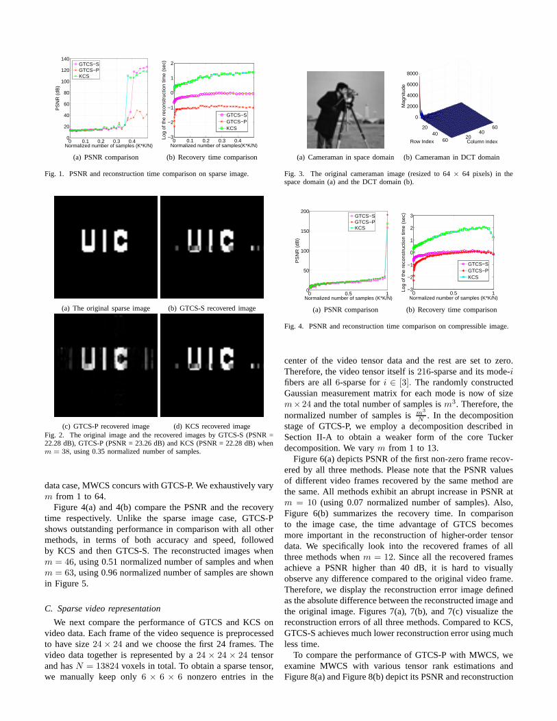
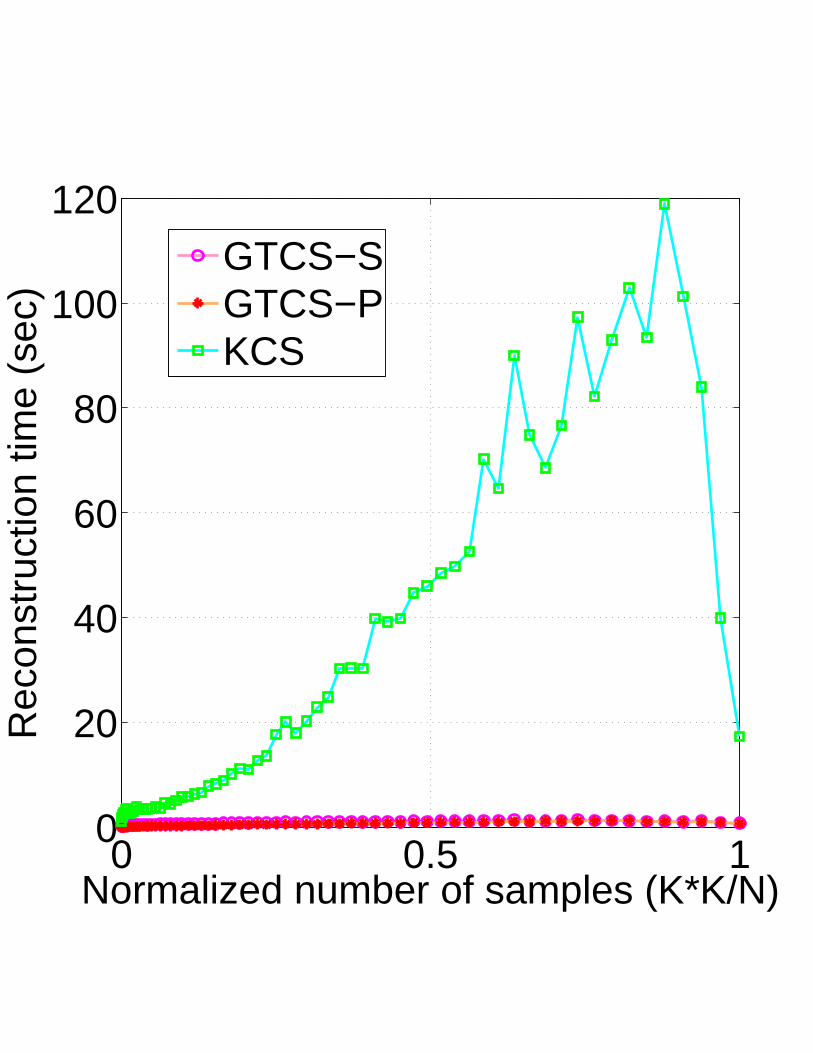
As shown in Figure 2(a), the original black and white imageis of size 64 × 64 (N = 4096 pixels). Its columns are14-sparse and rows are18-sparse. The image itself is178-sparse.We let the number of measurements evenly split among thetwo modes, that is, for each mode, the randomly constructedGaussian matrixU is of size m × 64. Therefore the KCSmeasurement matrixU⊗U is of sizem2×4096. Thus the totalnumber of samples ism2. We define the normalized number ofsamples to bem

2

N. For GTCS, both the serial recovery method

GTCS-S and the parallelizable recovery method GTCS-P areimplemented. In the matrix case, GTCS-P coincides withMWCS and we simply conduct SVD on the compressedimage in the decomposition stage of GTCS-P. Although thereconstruction stage of GTCS-P is parallelizable, we hererecover each vector in series. We comprehensively examinethe performance of all the above methods by varyingm from1 to 45.

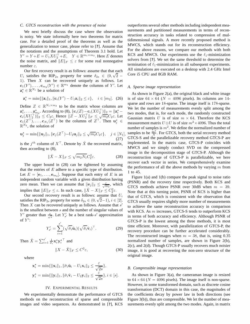
Figure 1(a) and 1(b) compare the peak signal to noise ratio(PSNR) and the recovery time respectively. Both KCS andGTCS methods achieve PSNR over 30dB whenm = 39.Note that at this turning point, PSNR of KCS is higher thanthat of GTCS, which is consistent with the observation thatGTCS usually requires slightly more number of measurementsto achieve the same reconstruction accuracy in comparisonwith KCS. Asm increases, GTCS-S tends to outperform KCSin terms of both accuracy and efficiency. Although PSNR ofGTCS-P is the lowest among the three methods, it is mosttime efficient. Moreover, with parallelization of GTCS-P, therecovery procedure can be further accelerated considerably.The reconstructed images whenm = 38, that is, using 0.35normalized number of samples, are shown in Figure 2(b),2(c), and 2(d). Though GTCS-P usually recovers much noisierimage, it is good at recovering the non-zero structure of theoriginal image.

B. Compressible image representation

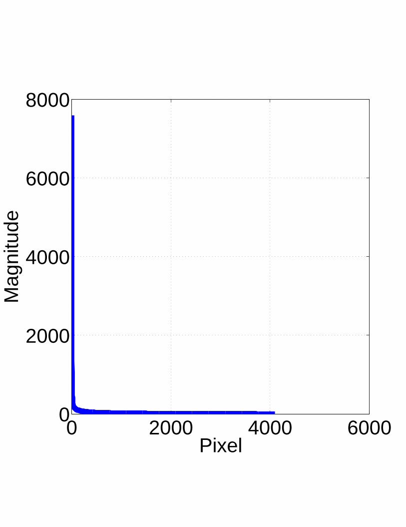
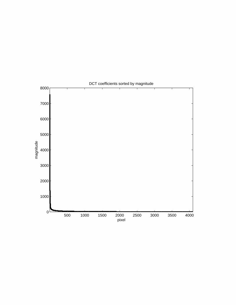
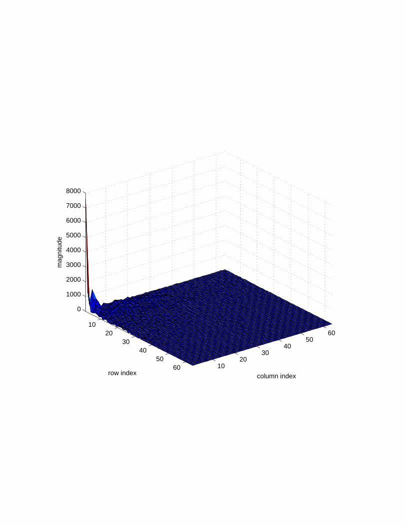
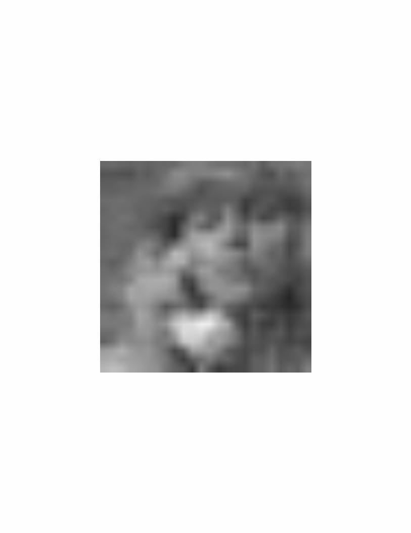
As shown in Figure 3(a), the cameraman image is resizedto 64× 64 (N = 4096 pixels). The image itself is non-sparse.However, in some transformed domain, such as discrete cosinetransformation (DCT) domain in this case, the magnitudes ofthe coefficients decay by power law in both directions (seeFigure 3(b)), thus are compressible. We let the number of mea-surements evenly split among the two modes. Again, in matrix

0 0.1 0.2 0.3 0.40

20

40

60

80

100

120

140

Normalized number of samples (K*K/N)

PS

NR

(dB

)

GTCS−SGTCS−PKCS

(a) PSNR comparison

0 0.1 0.2 0.3 0.4−3

−2

−1

0

1

2

Normalized number of samples(K*K/N)

Log

of th

e re

cons

truc

tion

time

(sec

)

GTCS−SGTCS−PKCS

(b) Recovery time comparison

Fig. 1. PSNR and reconstruction time comparison on sparse image.

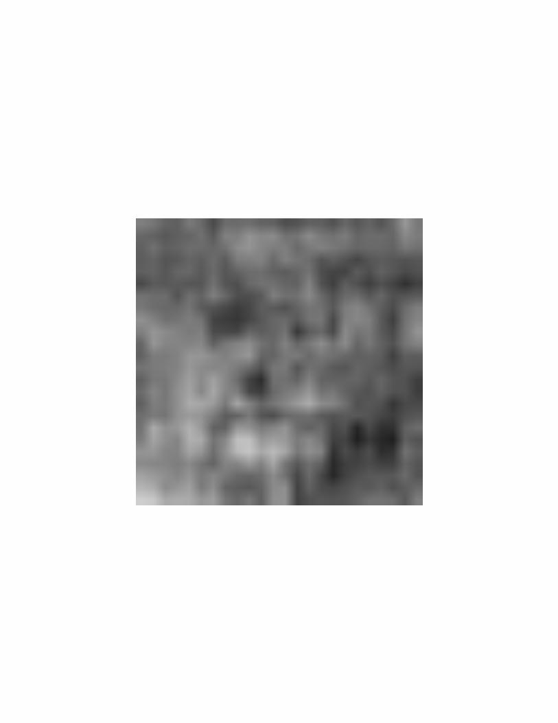
(a) The original sparse image (b) GTCS-S recovered image

(c) GTCS-P recovered image (d) KCS recovered imageFig. 2. The original image and the recovered images by GTCS-S(PSNR =22.28 dB), GTCS-P (PSNR = 23.26 dB) and KCS (PSNR = 22.28 dB) whenm = 38, using 0.35 normalized number of samples.

data case, MWCS concurs with GTCS-P. We exhaustively varym from 1 to 64.

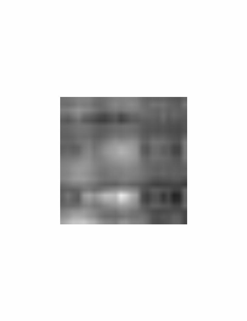
Figure 4(a) and 4(b) compare the PSNR and the recoverytime respectively. Unlike the sparse image case, GTCS-Pshows outstanding performance in comparison with all othermethods, in terms of both accuracy and speed, followedby KCS and then GTCS-S. The reconstructed images whenm = 46, using 0.51 normalized number of samples and whenm = 63, using 0.96 normalized number of samples are shownin Figure 5.

C. Sparse video representation

We next compare the performance of GTCS and KCS onvideo data. Each frame of the video sequence is preprocessedto have size24× 24 and we choose the first 24 frames. Thevideo data together is represented by a24 × 24 × 24 tensorand hasN = 13824 voxels in total. To obtain a sparse tensor,we manually keep only6 × 6 × 6 nonzero entries in the

(a) Cameraman in space domain

2040

602040

60

0

2000

4000

6000

8000

Column indexRow Index

Mag

nitu

de

(b) Cameraman in DCT domain

Fig. 3. The original cameraman image (resized to 64× 64 pixels) in thespace domain (a) and the DCT domain (b).

0 0.5 10

50

100

150

200

Normalized number of samples (K*K/N)P

SN

R (

dB)

GTCS−SGTCS−PKCS

(a) PSNR comparison

0 0.5 1−3

−2

−1

0

1

2

3

Normalized number of samples (K*K/N)

Log

of th

e re

cons

truc

tion

time

(sec

)

GTCS−SGTCS−PKCS

(b) Recovery time comparison

Fig. 4. PSNR and reconstruction time comparison on compressible image.

center of the video tensor data and the rest are set to zero.Therefore, the video tensor itself is216-sparse and its mode-i

fibers are all6-sparse fori ∈ [3]. The randomly constructedGaussian measurement matrix for each mode is now of sizem× 24 and the total number of samples ism3. Therefore, thenormalized number of samples ism

3

N. In the decomposition

stage of GTCS-P, we employ a decomposition described inSection II-A to obtain a weaker form of the core Tuckerdecomposition. We varym from 1 to 13.

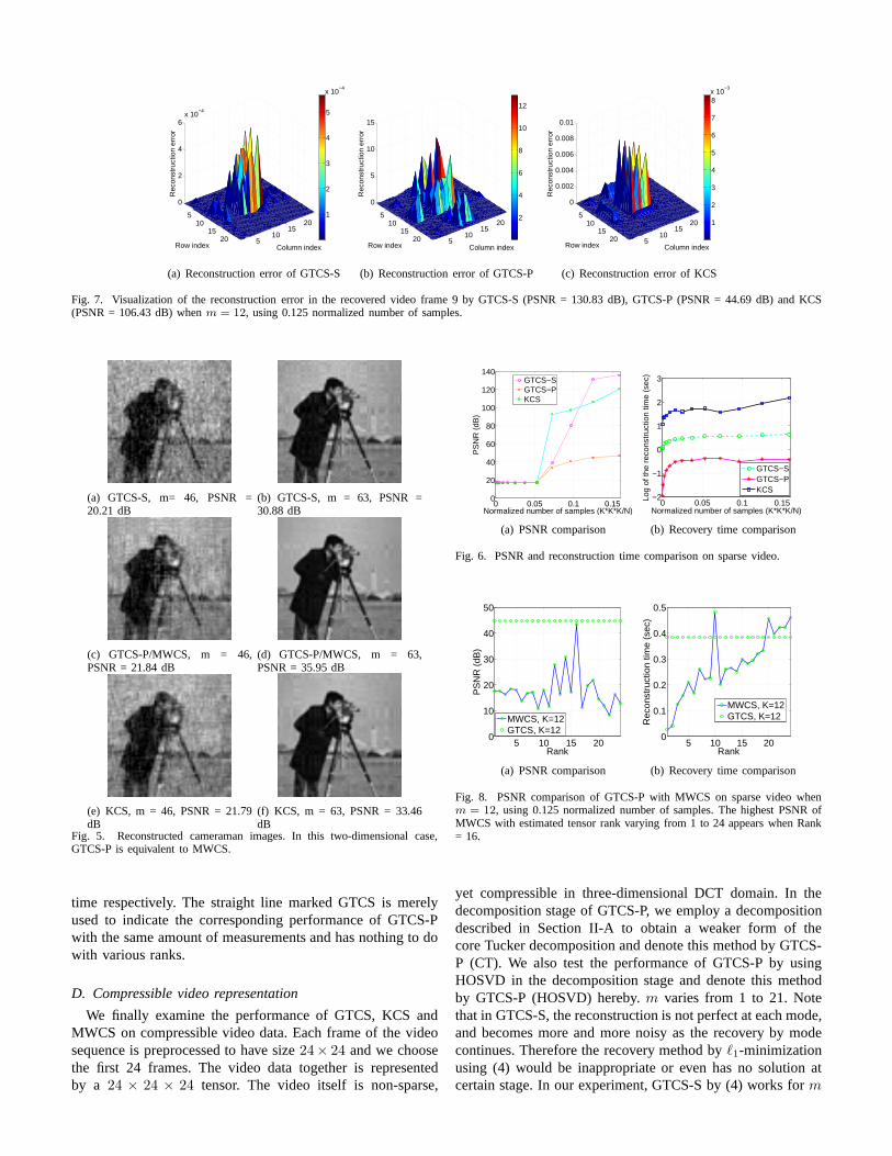
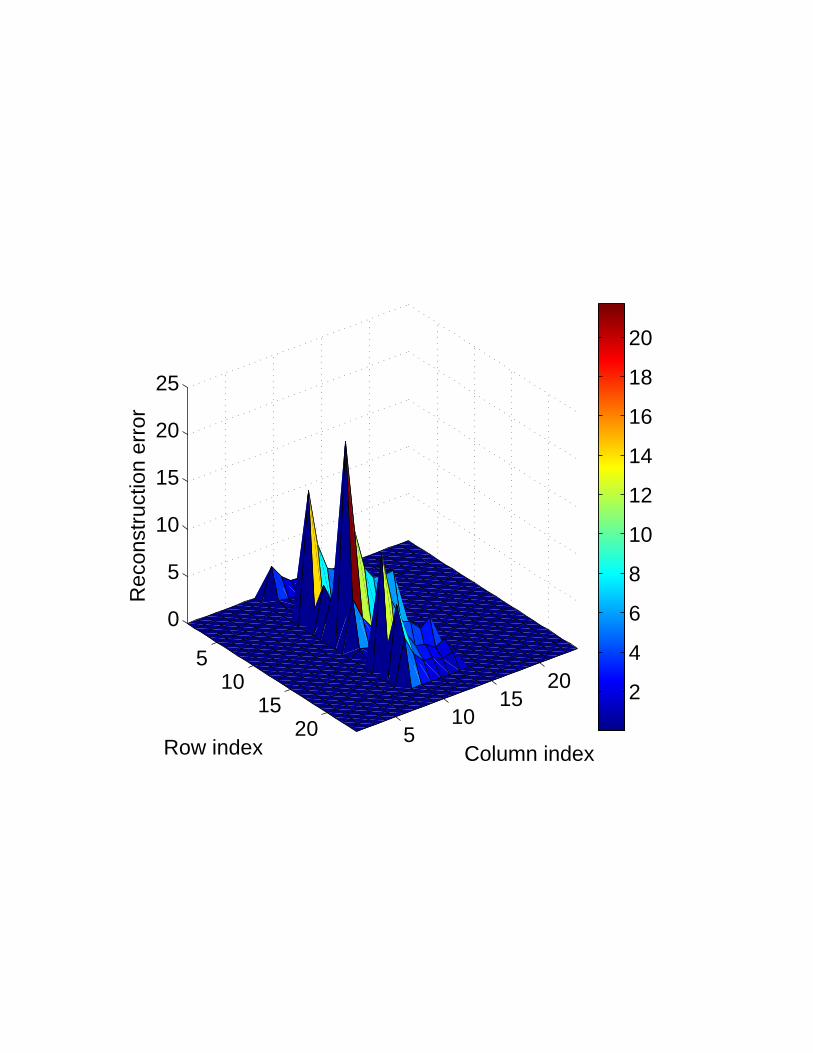
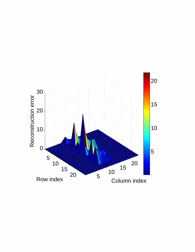
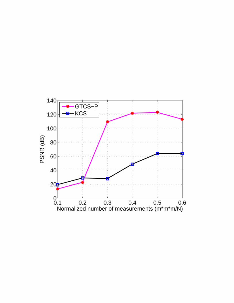
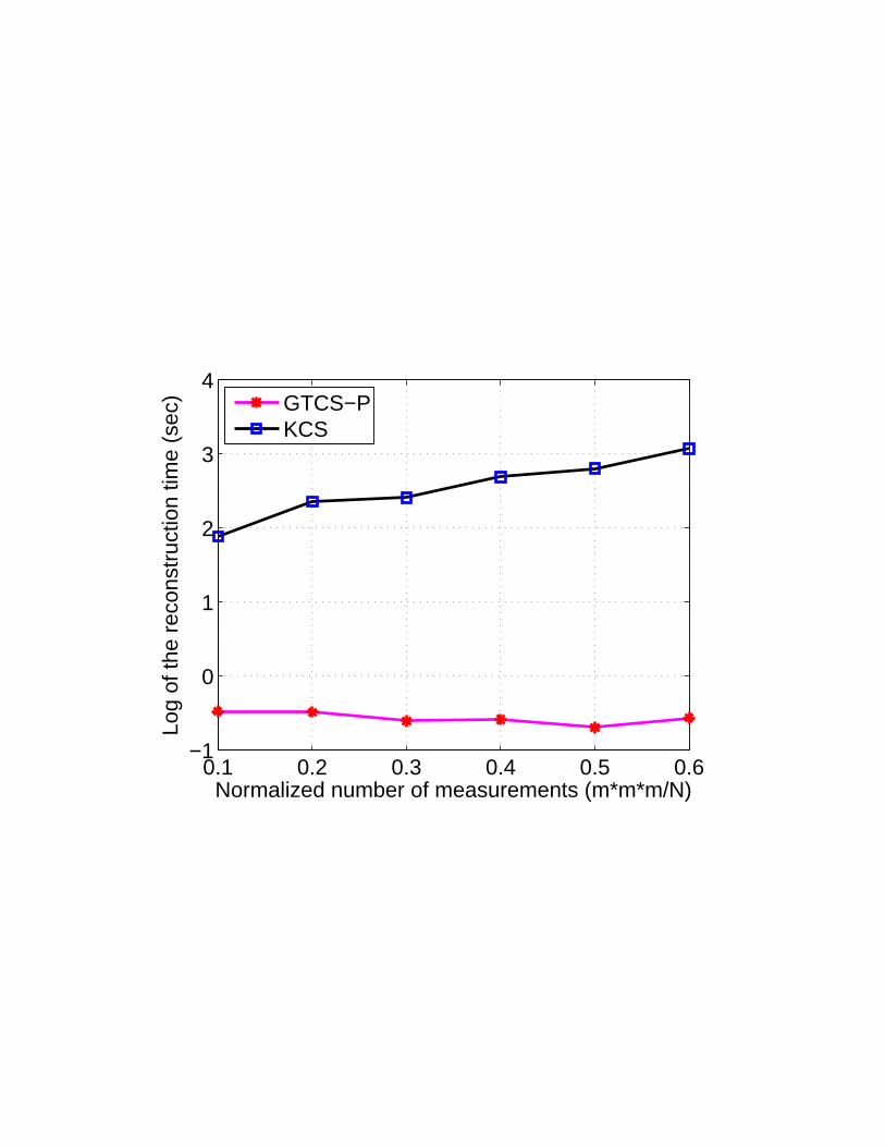
Figure 6(a) depicts PSNR of the first non-zero frame recov-ered by all three methods. Please note that the PSNR valuesof different video frames recovered by the same method arethe same. All methods exhibit an abrupt increase in PSNR atm = 10 (using 0.07 normalized number of samples). Also,Figure 6(b) summarizes the recovery time. In comparisonto the image case, the time advantage of GTCS becomesmore important in the reconstruction of higher-order tensordata. We specifically look into the recovered frames of allthree methods whenm = 12. Since all the recovered framesachieve a PSNR higher than 40 dB, it is hard to visuallyobserve any difference compared to the original video frame.Therefore, we display the reconstruction error image definedas the absolute difference between the reconstructed imageandthe original image. Figures 7(a), 7(b), and 7(c) visualize thereconstruction errors of all three methods. Compared to KCS,GTCS-S achieves much lower reconstruction error using muchless time.

To compare the performance of GTCS-P with MWCS, weexamine MWCS with various tensor rank estimations andFigure 8(a) and Figure 8(b) depict its PSNR and reconstruction

510

1520

510

1520

0

2

4

6x 10

−4

Column indexRow index

Rec

onst

ruct

ion

erro

r

1

2

3

4

5

x 10−4

(a) Reconstruction error of GTCS-S

510

1520

510

1520

0

5

10

15

Column indexRow index

Rec

onst

ruct

ion

erro

r

2

4

6

8

10

12

(b) Reconstruction error of GTCS-P

510

1520

510

1520

0

0.002

0.004

0.006

0.008

0.01

Column indexRow index

Rec

onst

ruct

ion

erro

r

1

2

3

4

5

6

7

8x 10

−3

(c) Reconstruction error of KCS

Fig. 7. Visualization of the reconstruction error in the recovered video frame 9 by GTCS-S (PSNR = 130.83 dB), GTCS-P (PSNR = 44.69 dB) and KCS(PSNR = 106.43 dB) whenm = 12, using 0.125 normalized number of samples.

(a) GTCS-S, m= 46, PSNR =20.21 dB

(b) GTCS-S, m = 63, PSNR =30.88 dB

(c) GTCS-P/MWCS, m = 46,PSNR = 21.84 dB

(d) GTCS-P/MWCS, m = 63,PSNR = 35.95 dB

(e) KCS, m = 46, PSNR = 21.79dB

(f) KCS, m = 63, PSNR = 33.46dB

Fig. 5. Reconstructed cameraman images. In this two-dimensional case,GTCS-P is equivalent to MWCS.

time respectively. The straight line marked GTCS is merelyused to indicate the corresponding performance of GTCS-Pwith the same amount of measurements and has nothing to dowith various ranks.

D. Compressible video representation

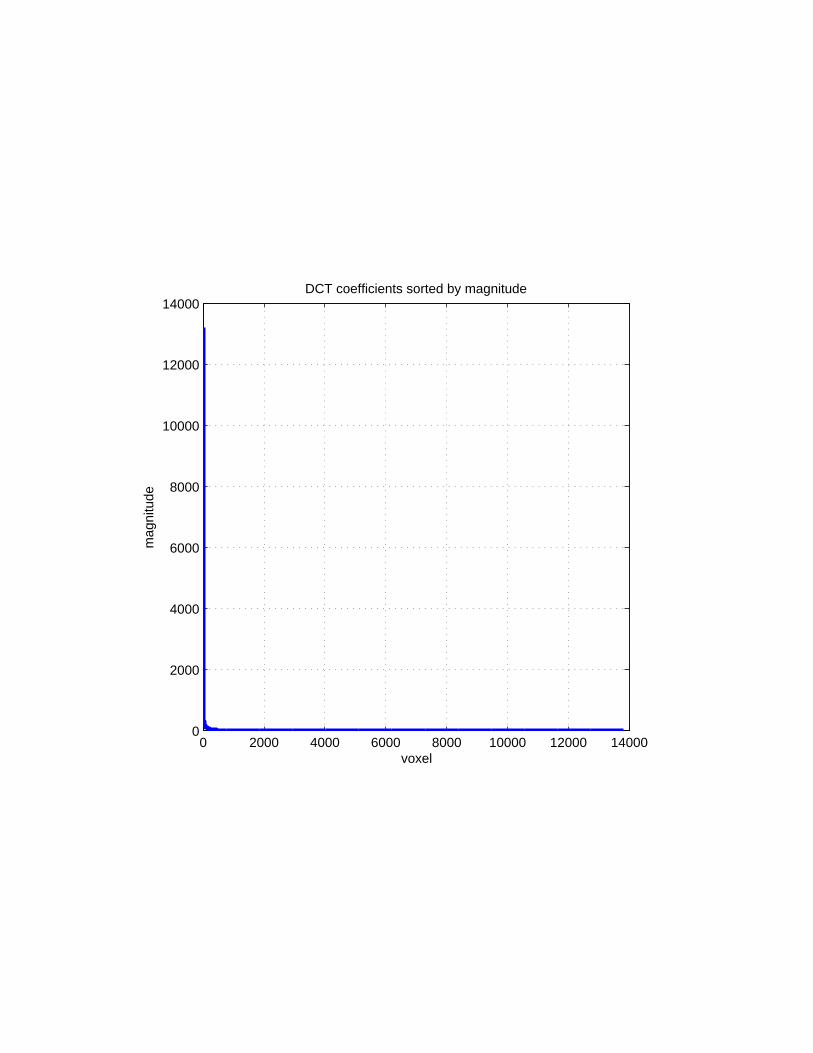
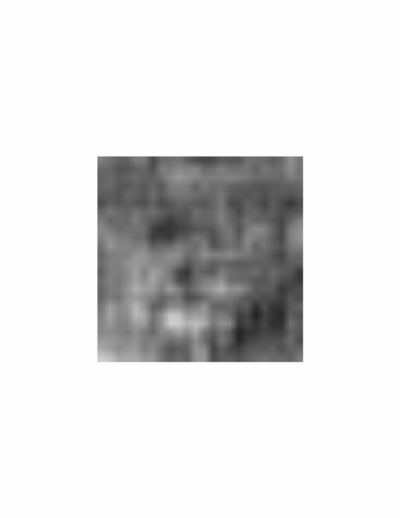
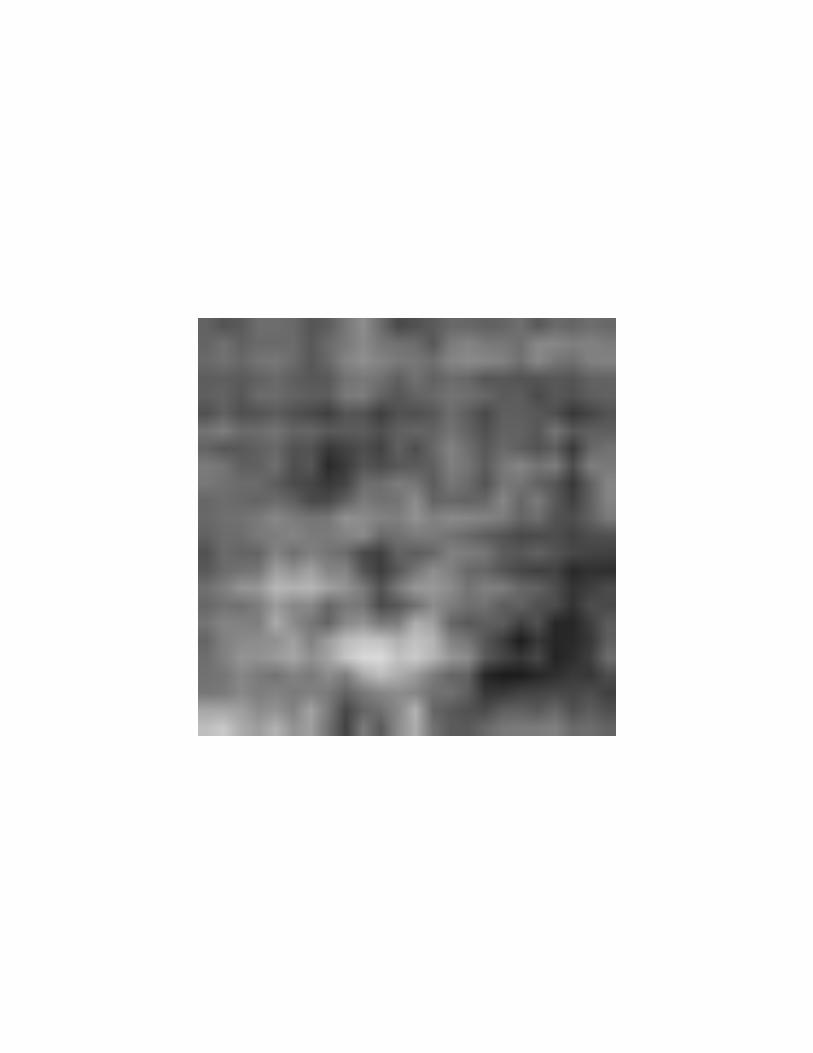
We finally examine the performance of GTCS, KCS andMWCS on compressible video data. Each frame of the videosequence is preprocessed to have size24× 24 and we choosethe first 24 frames. The video data together is representedby a 24 × 24 × 24 tensor. The video itself is non-sparse,

0 0.05 0.1 0.150

20

40

60

80

100

120

140

Normalized number of samples (K*K*K/N)

PS

NR

(dB

)

GTCS−SGTCS−PKCS

(a) PSNR comparison

0 0.05 0.1 0.15−2

−1

0

1

2

3

Normalized number of samples (K*K*K/N)

Log

of th

e re

cons

truc

tion

time

(sec

)

GTCS−SGTCS−PKCS

(b) Recovery time comparison

Fig. 6. PSNR and reconstruction time comparison on sparse video.

5 10 15 200

10

20

30

40

50

Rank

PS

NR

(dB

)

MWCS, K=12GTCS, K=12

(a) PSNR comparison

5 10 15 200

0.1

0.2

0.3

0.4

0.5

Rank

Rec

onst

ruct

ion

time

(sec

)

MWCS, K=12GTCS, K=12

(b) Recovery time comparison

Fig. 8. PSNR comparison of GTCS-P with MWCS on sparse video whenm = 12, using 0.125 normalized number of samples. The highest PSNRofMWCS with estimated tensor rank varying from 1 to 24 appears when Rank= 16.

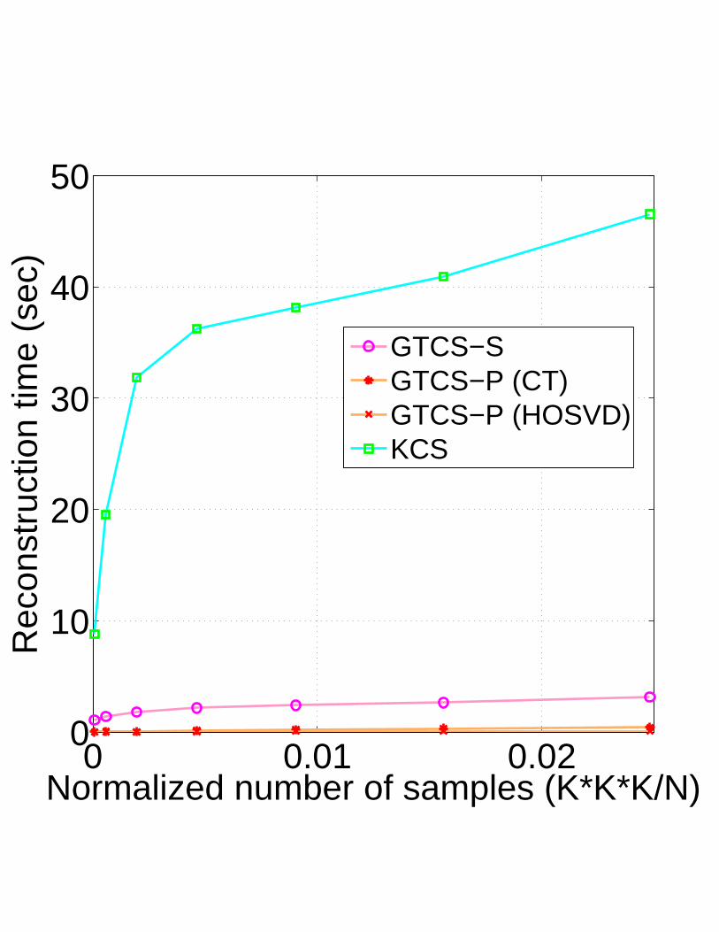
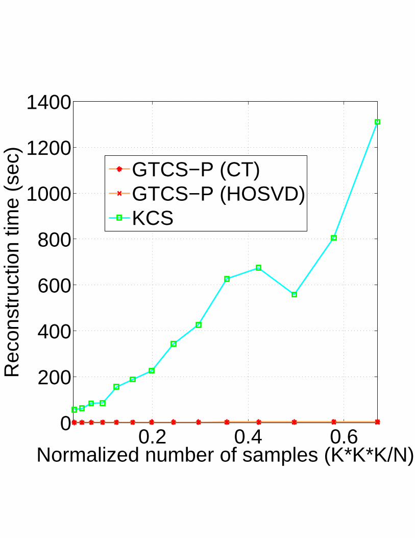
yet compressible in three-dimensional DCT domain. In thedecomposition stage of GTCS-P, we employ a decompositiondescribed in Section II-A to obtain a weaker form of thecore Tucker decomposition and denote this method by GTCS-P (CT). We also test the performance of GTCS-P by usingHOSVD in the decomposition stage and denote this methodby GTCS-P (HOSVD) hereby.m varies from 1 to 21. Notethat in GTCS-S, the reconstruction is not perfect at each mode,and becomes more and more noisy as the recovery by modecontinues. Therefore the recovery method byℓ1-minimizationusing (4) would be inappropriate or even has no solution atcertain stage. In our experiment, GTCS-S by (4) works form

from 1 to 7. To use GTCS-S form = 8 and higher, relaxedrecovery (7) could be employed for reconstruction. Figure 9(a)and Figure 9(b) depict PSNR and reconstruction time of allmethods up tom = 7. Form = 8 to 21, the results are shownin Figure 9(c) and Figure 9(d).

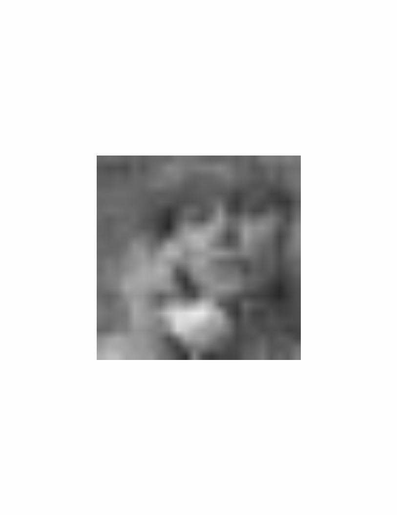
We specifically look into the recovered frames of all meth-ods whenm = 17 and m = 21. Recovered frames 1,9, 17 (originally as shown in Figure 10) are depicted asan example in Figure 11. As shown in Figure 12(a), the

0 0.01 0.026

8

10

12

14

16

18

Normalized number of samples (K*K*K/N)

PS

NR

(dB

)

GTCS−SGTCS−P (CT)GTCS−P (HOSVD)KCS

(a) PSNR comparison

0 0.01 0.02−2

−1

0

1

2

Normalized number of samples (K*K*K/N)

Log

of th

e re

cons

truc

tion

time

(sec

)

GTCS−SGTCS−P (CT)GTCS−P (HOSVD)KCS

(b) Recovery time comparison

0.2 0.4 0.615

20

25

30

35

Normalized number of samples (K*K*K/N)

PS

NR

(dB

)

GTCS−P (CT)GTCS−P (HOSVD)KCS

(c) PSNR comparison

0 0.2 0.4 0.6−2

−1

0

1

2

3

4

Normalized number of samples (K*K*K/N)

Log

of th

e re

cons

truc

tion

time

(sec

)

GTCS−P (CT)GTCS−P (HOSVD)KCS

(d) Recovery time comparisonFig. 9. PSNR and reconstruction time comparison on susie video.

(a) Original frame 1 (b) Original frame 9 (c) Original frame 17

Fig. 10. Original video frames.

performance of MWCS relies highly on the estimation of thetensor rank. We examine the performance of MWCS withvarious rank estimations. Experimental results demonstratethat GTCS outperforms MWCS not only in speed, but alsoin accuracy.

V. CONCLUSION

Extensions of CS theory to multidimensional signals havebecome an emerging topic. Existing methods include Kro-necker compressive sensing (KCS) for sparse tensors andmulti-way compressive sensing (MWCS) for sparse and low-rank tensors. We introduced the Generalized Tensor Compres-sive Sensing (GTCS)–a unified framework for compressivesensing of higher-order tensors which preserves the intrinsicstructure of tensorial data with reduced computational com-plexity at reconstruction. We demonstrated that GTCS offers

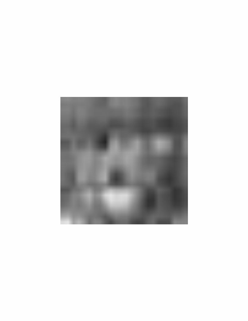
(a) GTCS-P(HOSVD)reconstructed frame 1

(b) GTCS-P(HOSVD)reconstructed frame 9

(c) GTCS-P(HOSVD)reconstructed frame 17

(d) GTCS-P(CT) recon-structed frame 1

(e) GTCS-P(CT) recon-structed frame 9

(f) GTCS-P(CT) recon-structed frame 17

(g) KCS reconstructedframe 1

(h) KCS reconstructedframe 9

(i) KCS reconstructedframe 17

(j) MWCS reconstructedframe 1

(k) MWCS reconstructedframe 9

(l) MWCS reconstructedframe 17

Fig. 11. Reconstructed video frames when m = 21 using 0.67 normalizednumber of samples by GTCS-P (HOSVD, PSNR = 29.33 dB), GTCS-P (CT,PSNR = 28.79 dB), KCS (PSNR = 30.70 dB) and MWCS (Rank = 4, PSNR= 22.98 dB).

5 10 15 20−10

0

10

20

30

Rank

PS

NR

(dB

)

MWCS, K=17GTCS, K=17MWCS, K=21GTCS, K=21

(a) PSNR comparison

5 10 15 200

0.2

0.4

0.6

0.8

1

Rank

Rec

onst

ruct

ion

time

(sec

)

MWCS, K=17GTCS, K=17MWCS, K=21GTCS, K=21

(b) Recovery time comparison

Fig. 12. PSNR comparison of GTCS-P with MWCS on compressiblevideowhen m = 17, using 0.36 normalized number of samples andm = 21,using 0.67 normalized number of samples. The highest PSNR ofMWCSwith estimated tensor rank varying from 1 to 24 appears when Rank = 4 andRank = 7 respectively.

an efficient means for representation of multidimensional databy providing simultaneous acquisition and compression fromall tensor modes. We introduced two reconstruction proce-dures, a serial method (GTCS-S) and a parallelizable method(GTCS-P), and compared the performance of the proposedmethods with KCS and MWCS. As shown, GTCS outperformsKCS and MWCS in terms of both reconstruction accuracy(within a range of compression ratios) and processing speed.

The major disadvantage of our methods (and of MWCS aswell), is that the achieved compression ratios may be worsethan those offered by KCS. GTCS is advantageous relativeto vectorization-based compressive sensing methods such asKCS because the corresponding recovery problems are interms of a multiple small measurement matricesUi’s, insteadof a single, large measurement matrixA, which results ingreatly reduced complexity. In addition, GTCS-P does notrely on tensor rank estimation, which considerably reducesthecomputational complexity while improving the reconstructionaccuracy in comparison with other tensorial decomposition-based method such as MWCS.

ACKNOWLEDGMENT

The authors would like to thank Dr. Edgar A. Bernal withPARC for his help with the simulation as well as shaping thepaper. We also want to extend our thanks to the anonymousreviewers for their constructive suggestions.

Shmuel Friedland received all his degrees in Math-ematics from Israel Institute of Technology,(IIT),Haifa, Israel: B.Sc in 1967, M.Sc. in 1969, D.Sc.in 1971. He held Postdoc positions in WeizmannInstitute of Science, Israel; Stanford University; IAS,Princeton. From 1975 to 1985, he was a member ofInstitute of Mathematics, Hebrew U., Jerusalem, andwas promoted to the rank of Professor in 1982. Since1985 he is a Professor at University of Illinois atChicago. He was a visiting Professor in Universityof Wisconsin; Madison; IMA, Minneapolis; IHES,

Bures-sur-Yvette; IIT, Haifa; Berlin Mathematical School, Berlin. Friedlandcontributed to the following fields of mathematics: one complex variable,matrix and operator theory, numerical linear algebra, combinatorics, ergodictheory and dynamical systems, mathematical physics, mathematical biology,algebraic geometry. He authored about 170 papers, with manyknown coau-thors, including one Fields Medal winner. He received the first Hans Schneiderprize in Linear Algebra, jointly with M. Fiedler and I. Gohberg, in 1993. Hewas awarded recently a smoked salmon for solving the set-theoretic versionof the salmon problem: http://www.dms.uaf.edu/∼eallman. For more detailson Friedland vita and research, see http://www.math.uic.edu/∼friedlan.

Qun Li received the B.S. degree in CommunicationsEngineering from Nanjing University of Science andTechnology, China, in 2009 and the M.S. and Ph.D.degrees in Electrical Engineering from University ofIllinois at Chicago (UIC), U.S.A. in 2012 and 2013respectively. She joined PARC, Xerox Corporation,NY, U.S.A. in 2013 as a research scientist aftergraduation. Her research interests include machinelearning, computer vision, image and video analysis,higher-order data analysis, compressive sensing, 3Dimaging, etc.

Dan Schonfeld received the B.S. degree in elec-trical engineering and computer science from theUniversity of California, Berkeley, and the M.S. andPh.D. degrees in electrical and computer engineeringfrom the Johns Hopkins University, Baltimore, MD,in 1986, 1988, and 1990, respectively. He joinedUniversity of Illinois at Chicago in 1990, wherehe is currently a Professor in the Departments ofElectrical and Computer Engineering, Computer Sci-ence, and Bioengineering, and Co-Director of theMultimedia Communications Laboratory (MCL). He

has authored over 170 technical papers in various journals and conferences.

0 2000 4000 60000

2000

4000

6000

8000

Pixel

Mag

nitu

de

0 0.5 10

20

40

60

80

100

120

Normalized number of samples (K*K/N)

Rec

onst

ruct

ion

time

(sec

)

GTCS−SGTCS−PKCS

500 1000 1500 2000 2500 3000 3500 40000

1000

2000

3000

4000

5000

6000

7000

8000

pixel

mag

nitu

de

DCT coefficients sorted by magnitude

0 2000 4000 6000 8000 10000 12000 140000

2000

4000

6000

8000

10000

12000

14000

voxel

mag

nitu

de

DCT coefficients sorted by magnitude

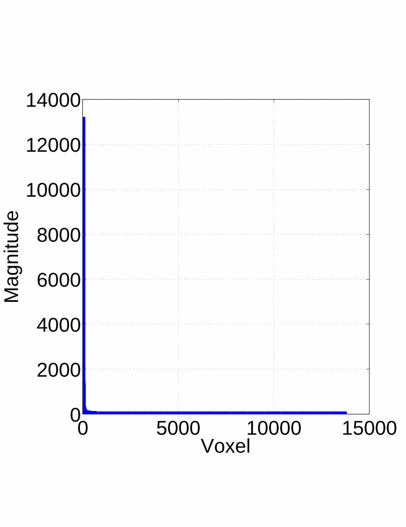
0 5000 10000 150000

2000

4000

6000

8000

10000

12000

14000

Voxel

Mag

nitu

de

1020

3040

5060

1020

3040

5060

0

1000

2000

3000

4000

5000

6000

7000

8000

column indexrow index

mag

nitu

de

0 0.01 0.020

10

20

30

40

50

Normalized number of samples (K*K*K/N)

Rec

onst

ruct

ion

time

(sec

)

GTCS−SGTCS−P (CT)GTCS−P (HOSVD)KCS

510

1520

510

1520

0

5

10

15

20

25

Column indexRow index

Rec

onst

ruct

ion

erro

r

2

4

6

8

10

12

14

16

18

20

510

1520

510

1520

0

10

20

30

Column indexRow index

Rec

onst

ruct

ion

erro

r

5

10

15

20

0.2 0.4 0.60

200

400

600

800

1000

1200

1400

Normalized number of samples (K*K*K/N)

Rec

onst

ruct

ion

time

(sec

)

GTCS−P (CT)GTCS−P (HOSVD)KCS

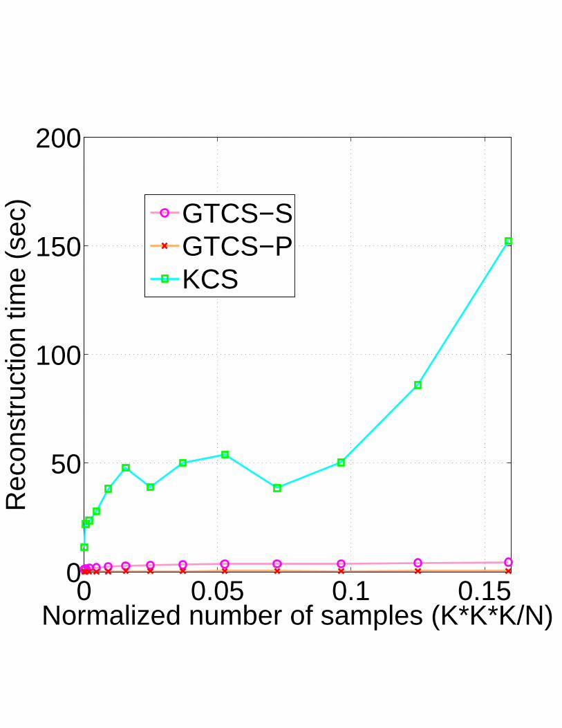
0 0.05 0.1 0.150

50

100

150

200

Normalized number of samples (K*K*K/N)

Rec

onst

ruct

ion

time

(sec

)

GTCS−SGTCS−PKCS

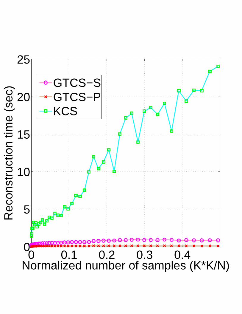
0 0.1 0.2 0.3 0.40

5

10

15

20

25

Normalized number of samples (K*K/N)

Rec

onst

ruct

ion

time

(sec

)

GTCS−SGTCS−PKCS

0.1 0.2 0.3 0.4 0.5 0.60

20

40

60

80

100

120

140

Normalized number of measurements (m*m*m/N)

PS

NR

(dB

)

GTCS−PKCS

0.1 0.2 0.3 0.4 0.5 0.6−1

0

1

2

3

4

Normalized number of measurements (m*m*m/N)

Log

of th

e re

cons

truc

tion

time

(sec

)

GTCS−PKCS