Embed Size (px)
Citation preview
Map Learning with Uninterpreted Sensors and Effectors�
David Pierce and Benjamin KuipersDepartment of Computer Sciences
University of Texas at Austin, Austin, TX 78712 [email protected] , [email protected]
Artificial Intelligence92: 169–229, 1997.
Abstract
This paper presents a set of methods by which a learning agent can learn a sequence of increasingly abstract andpowerful interfaces to control a robot whose sensorimotor apparatus and environment are initially unknown. Theresult of the learning is a rich hierarchical model of the robot’s world (its sensorimotor apparatus and environment).The learning methods rely on generic properties of the robot’s world such as almost-everywhere smooth effectsof motor control signals on sensory features. At the lowest level of the hierarchy, the learning agent analyzes theeffects of its motor control signals in order to define a new set of control signals, one for each of the robot’s degreesof freedom. It uses a generate-and-test approach to define sensory features that capture important aspects of theenvironment. It uses linear regression to learn models that characterize context-dependent effects of the controlsignals on the learned features. It uses these models to define high-level control laws for finding and following pathsdefined using constraints on the learned features. The agent abstracts these control laws, which interact with thecontinuous environment, to a finite set of actions that implement discrete state transitions. At this point, the agenthas abstracted the robot’s continuous world to a finite-state world and can use existing methods to learn its structure.The learning agent’s methods are evaluated on several simulated robots with different sensorimotor systems andenvironments.
Keywords: spatial semantic hierarchy, map learning, cognitive maps, feature learning, abstract interfaces, actionmodels, changes of representation.
�This work has taken place in the Qualitative Reasoning Group at the Artificial Intelligence Laboratory, The University of Texas at Austin.Research of the Qualitative Reasoning Group is supported in part by NSF grants IRI-9216584 and IRI-9504138, by NASA grants NCC 2-760 andNAG 2-994, and by the Texas Advanced Research Program under grant no. 003658-242.
1

Pierce & Kuipers, AIJ, 1997 2
Sensory input Control
Figure 1:The learning problem addressed in this paper is illustrated by this interface between a learning agent and a teleoperatedrobot in an unknown environment. The learning agent’s problem is to learn a model of the robot and its environment with no initialknowledge of the meanings of the sensors or the effects of the control signals (except that nothing changes when the control signalsare all zero).
1 Introduction
Suppose a creature emerges into an unknown environment, with no knowledge of what its sensors are sensing or whatits effectors are effecting. How can such a creature learn enough about its sensors and effectors to learn about thenature of its environment? What primitive capabilities are sufficient to support such a learning process?
This problem is idealized to clarify the goals and results of our research. A real robot embodies knowledgedesigned and programmed in by engineers who select sensors and effectors appropriate to the environment, and im-plement control laws appropriate to the goals of the robot. A real biological organism embodies knowledge, acquiredthrough evolution, that matches the sensorimotor capabilities of the organism to the demands of the environment. Weidealize both of these to the problem faced by an individual learning agent with very little domain-specific knowledge,but with the ability to apply a number of sophisticated, domain-independent learning methods. In addition to its scien-tific value, this idealized learning agent would be of considerable practical value in allowing a newly-designed robotto learn the properties of its own sensorimotor system. We report here on one learning agent that solves a specific in-stance of this problem, along with several variations that begin to explore the range of possible solutions to the generalproblem.
Henceforth, we make a distinction between the learning agent and the robot. The robot is a machine (physical orsimulated) that the learning agent must learn how to use. The robot’s sensorimotor apparatus is comprised of a set ofsensors and effectors. The sensorimotor apparatus isuninterpreted, meaning that the agent that is learning how to usethe robot has noa priori knowledge of the meaning of the sensors, of the structure of the sensory system, or of theeffects of the motor’s control signals. From the learning agent’s perspective, the sensorimotor apparatus is representedas araw sense vectors and araw motor control vectoru. The former is a vector of real numbers giving the currentvalues of all of the sensors. The latter is a vector of real numbers, called control signals, produced by the learningagent and sent to the robot’s motor apparatus. The learning agent’s situation is illustrated in Figure 1.
This paper solves the learning problem by presenting a set of methods that the learning agent can use to learn (1) amodel of the robot’s set of sensors, (2) a model of the robot’s motor apparatus, and (3) a set of behaviors that allow thelearning agent to abstract the robot’s continuous world to a discrete world of places and paths. These methods havebeen demonstrated on a simulated mobile robot with a ring of distance sensors.
These learning methods comprise a body of knowledge that is given to the learning agenta priori. They incorpo-rate a knowledge of basic mathematics, multivariate analysis, and control theory. The learning methods are domainindependent in that they are not based on a particular set of sensors or effectors and do not make assumptions aboutthe structure or even the dimensionality of the robot’s environment.
In the rest of this paper, we describe a number of learning methods and show how they are used by a learning agentas it develops an understanding of a robot’s world by defining a sequence of increasingly powerfulabstract interfacesto the robot. The learning agent’s problem and solution are given below:
Problem

Pierce & Kuipers, AIJ, 1997 3
Given: a robot with an uninterpreted,almost-everywhere approximately linearsensorimotor apparatus in acontinuous, staticenvironment.
Learn: descriptions of the structure of the robot’s sensorimotor apparatus and environment and an abstractinterface to the robot suitable forpredictionandnavigation.
SolutionRepresentation: a hierarchical model. At the bottom of the hierarchy are egocentric models of the robot’ssensorimotor apparatus. At the top of the hierarchy is a discrete abstraction of the robot’s environment definedby a set of discrete views and actions.
Method: a sequence of statistical and generate-and-test methods for learning the objects of the hierarchicalmodel.
An almost-everywhere approximately linearsensorimotor apparatus satisfies the following: The derivatives with re-spect to time of the sensor values can be approximated by linear functions of the motor control vector. Acontinuousworld (which includes both the robot and its environment) is one whose state can be represented by a vectorx ofcontinuous, real-valued state variables. Adiscreteworld, on the other hand, is represented by a finite set of states. Theprimary example in this paper1 is a mobile robot in a continuous world with three state variables: two for its position(e.g., longitude and latitude) and one for its orientation (i.e., the direction in which it is facing). Astaticworld is onewhose state does not change except as the result of a nonzero motor control vector. A static world exhibits no inertia.When the motor controls go to zero, the robot comes to an immediate stop. In a static world, there are no active agents(e.g., pedestrians) besides the robot itself.
The learning agent’s goal is to understand its world, that is, to learn a model of it suitable for prediction andnavigation. Prediction refers to the ability to predict the effects of the motor control signals.Navigation refersto the ability to move efficiently from one place to another. These definitions do not apply perfectly to the learn-ing agent’s world: places do not exista priori — they must be discovered or invented by the learning agent itself.The raw sense vector and the raw motor control vectors are at the wrong level of abstraction for describing theglobal structure of a world. People do not understand their world in terms of sequences of visual images — theyuse abstractions from visual scenes to places and objects. In order to understand its continuous world, the learningagent must also use abstractions. Instead of trying to make predictions based on the raw sense vector, it needs tolearn high-level features and behaviors. Understanding the world thus requires a hierarchy of features, behaviors,and accompanying descriptions. The hierarchy that the learning agent uses is called thespatial semantic hierarchy[Kuipers and Byun, 1988, Kuipers and Byun, 1991, Kuipers and Levitt, 1988, Kuipers, 1996].
1.1 The spatial semantic hierarchy
The spatial semantic hierarchy (SSH) is a hierarchical structure for a substantial body of commonsense knowledge,showing how acognitive mapcan be built on sensorimotor interaction with the world. The cognitive map is thebody of knowledge an agent has about the large-scale spatial structure of its environment. (“Large-scale” here meanssignificantly larger than the sensory horizon of the agent, meaning that the map must be constructed by integratingobservations over time as the agent travels through its environment.) Since we already have an SSH-based solution forthe cognitive mapping problem for a simulated robot with a ring of distance sensors, we focus on learning the sensoryfeatures and control strategies necessary to support that solution. The result we obtained was successful, but at thesame time revealed some subtle but important changes required to the SSH approach to cognitive mapping.2
The spatial semantic hierarchy is comprised of five levels: sensorimotor, control, causal, topological, and metrical.At the sensorimotorlevel, the abstract interface to the robot is defined by the raw sense vector, a set of primitiveactions (one for each degree of freedom of the robot, Section 3), and a set of learned features. At thecontrol level,action models are learned in order to predict the context-dependent effects of motor control vectors on features. Localstate variables are learned and behaviors for homing and path-following are defined (Section 5). The abstract interface
1Experiments with other robots are described in connection with particular learning methods.2The most important change is the use of local state variables (Section 4).

Pierce & Kuipers, AIJ, 1997 4
to the robot is defined by the set of local state variables, homing behaviors, and path-following behaviors. At thecausallevel, sense vectors are abstracted to a finite set ofviewsand behaviors are abstracted to a finite set ofactions(Section 7). The abstract interface gives the current view and the set of currently applicable actions.
The contribution of this paper is a set of methods for learning these first three levels. This paper’s work is comple-mentary to the work done by Kuipers and Byun [Kuipers and Byun, 1988, Kuipers and Byun, 1991] in which all levelsof the descriptive ontology were engineered by hand, and the focus of the learning agent was on learning the structureof the environment. The agent selected appropriate control laws from a fixed set to form the control level, which wasabstracted to the topological and metrical levels. At thetopologicallevel, perceptual ambiguities (in which multiplestates map to the same view) are resolved and a global representation of the world’s structure as a finite-state graphis learned. At themetrical level, the topological map is supplemented with distances, directions, and other metricalinformation.
By showing how to learn the first three levels of the spatial semantic hierarchy, this paper lays the groundwork forbuilding a learning agent that can learn the entire spatial semantic hierarchy using only domain-independent knowl-edge.
1.2 Overview
Sections 2 through 7 describe a sequence of methods for learning a model of a robot’s sensorimotor apparatus and aset of behaviors that allow the learning agent to abstract the robot’s continuous world to a discrete world of places andpaths. Figure 30 summarizes the entire set of representations, learning methods, and resulting behaviors, after theyhave been described in detail in the rest of the paper.
Section 2 describes a method for learning a model of the structure of the robot’s sensory apparatus. Section 3describes a method for learning a model of the structure of the robot’s motor apparatus. Section 4 describes a methodfor learning a set of variables suitable for representing the local state of the robot. Section 5 describes a method forlearning a set of robust, repeatable behaviors for navigation through the robot’s state space. Section 6 describes anumber of experiments (in addition to those described in the previous sections) that demonstrate the generality andsome limitations of these learning methods. Finally, Section 7 shows how to define an abstract interface that abstractsfrom the continuous sensorimotor apparatus to a discrete sensorimotor apparatus.
These learning methods provide a particular solution to the learning problem described in Section 1. This particularsolution is an instance of the more general solution outlined below:
1. Apply a generate-and-test algorithm to produce a set of scalar features.
2. Try to learn how to control the generated scalar features. Those that can be controlled are identified aslocalstate variables.
3. Definehoming behaviors— behaviors that move a local state variable to a target value.
4. Definepath-following behaviors— behaviors that move the robot while keeping a local state variable at itstarget value.
The set of learning methods that are presented in this paper does not represent the final word on the problem oflearning to use an uninterpreted sensorimotor apparatus. Instead it is one path to the goal. Clearly, there are otherways to instantiate the above sequence of steps. Future work will involve both improving the current set of methodsand identifying alternate paths to the solution.
The learning methods and experimental results are interleaved throughout the paper: each section describes alearning method, the representations or objects produced by the method, the source of information used by the method,and one or more demonstrations of the method applied to a simulated robot.
1.3 Contributions
The results of this research are the following:
Pierce & Kuipers, AIJ, 1997 5
1. the demonstration of a learning agent that can solve a nontrivial instance of the learning problem;
2. the identification of a plausible though not unique set of primitive capabilities that a robot must have to supportsuch a learning agent;
3. the identification of a set of learning methods and intermediate representations that enable the learning agent togo from no domain-specific knowledge to useful cognitive maps of complex environments.
These learning methods are interesting in their own right. First, each one identifies a source of information availablethrough experimentation with an uninterpreted sensorimotor apparatus and, second, each provides a method for ex-ploiting that information to give the learning agent a new way of understanding the robot’s sensory input or a new wayof interacting with the robot’s environment.
The result of this work is an existence proof, demonstrating one path from the beginning to the end of an ideal-ized but important learning problem. We hope that this result can support further work to establish minimal sets ofprimitives, necessary conditions for success, and the limits of this heterogeneous bootstrapping method for learning.
As intended, the learned set of features and control laws are specific to the robot and the type of environmentused for these experiments. The learning method itself also has some degree of dependence on the type of robotand environments used. We used three methods to move towards generality in these results. First, as we needed toadd primitive inference capabilities, we required that they be independent of the choice of robot or environment, andthat they be plausible to implement using low-level symbolic or neural-net mechanisms.3 Second, we attempted tominimize, and then make explicit, the assumptions our inference methods make about the nature of the robot or theenvironment. For example, several feature generators require almost-everywhere temporal and spatial continuity of thesensory inputs.4 Third, we tested the generality of several key steps in our learning method empirically by applyingthem to different robot sensorimotor systems and different environments. These results are shown throughout thepaper. Naturally, the generality we are able to establish by these means remains limited.
In spite of the limitations of an existence proof, we believe that the approach we have demonstrated is important.First, it shows how a heterogeneous set of learning methods can be used to construct a deep hierarchy of sensory fea-tures and control laws. Only a very few previous learning methods such as AM [Lenat, 1977] (see also [Shen, 1990])have constructed similarly deep concept hierarchies. Second, the knowledge contained in this hierarchy shows how afoundational domain of symbolic commonsense knowledge can be grounded in continuous sensorimotor interactionwith a continuous world.
2 Learning a model of the sensory apparatus
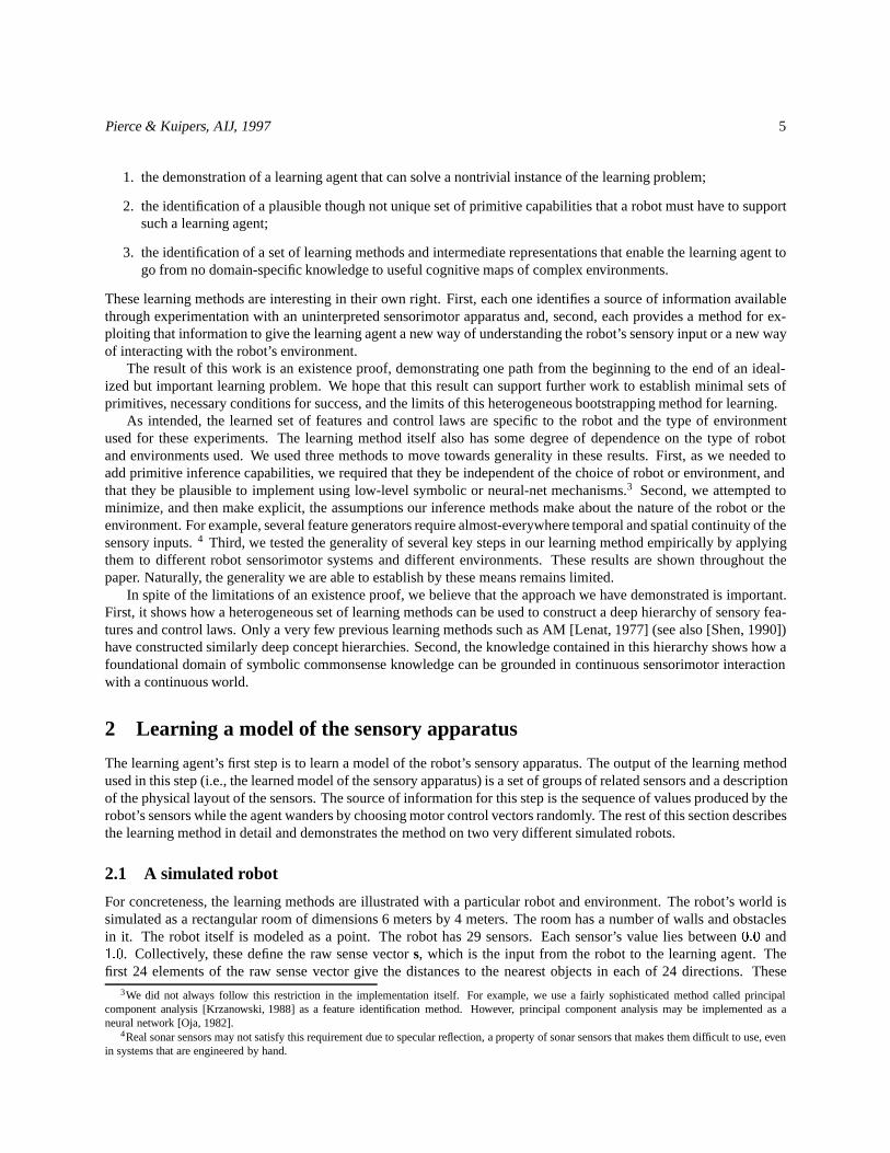
The learning agent’s first step is to learn a model of the robot’s sensory apparatus. The output of the learning methodused in this step (i.e., the learned model of the sensory apparatus) is a set of groups of related sensors and a descriptionof the physical layout of the sensors. The source of information for this step is the sequence of values produced by therobot’s sensors while the agent wanders by choosing motor control vectors randomly. The rest of this section describesthe learning method in detail and demonstrates the method on two very different simulated robots.
2.1 A simulated robot
For concreteness, the learning methods are illustrated with a particular robot and environment. The robot’s world issimulated as a rectangular room of dimensions 6 meters by 4 meters. The room has a number of walls and obstaclesin it. The robot itself is modeled as a point. The robot has 29 sensors. Each sensor’s value lies between0:0 and1:0. Collectively, these define the raw sense vectors, which is the input from the robot to the learning agent. Thefirst 24 elements of the raw sense vector give the distances to the nearest objects in each of 24 directions. These
3We did not always follow this restriction in the implementation itself. For example, we use a fairly sophisticated method called principalcomponent analysis [Krzanowski, 1988] as a feature identification method. However, principal component analysis may be implemented as aneural network [Oja, 1982].
4Real sonar sensors may not satisfy this requirement due to specular reflection, a property of sonar sensors that makes them difficult to use, evenin systems that are engineered by hand.
Pierce & Kuipers, AIJ, 1997 6
have a maximum value of 1.0, which they take on when the nearest object is beyond one meter away. The sonarsare numbered clockwise from the front. The 21st element is defective and always returns a value of 0.2. The 25thelement is a sensor giving the battery’s voltage, which decreases slowly from an initial value of 1.0. The 26th through29th elements comprise a digital compass. The element with value 1 corresponds to the direction (E, N, W, or S) inwhich the robot is most nearly facing. There is no sensor noise. The robot has a “tank-style” motor apparatus. Itstwo motor control signalsa0 anda1 tell how fast to move the right and left treads. Moving the treads together at thesame speed produces pure forward or backward motion; moving them in opposition at the same speed produces purerotation. Moving the treads at different speeds causes the robot to move in a circular arc. The learning agent does notknow what any of these sensors or effectors do. The learning agent only knows that that robot’s raw sense vector has29 elements and its raw motor control vector has two elements.
2.2 A language of features
The learning agent develops an understanding of the robot’s sensory apparatus by learning newfeatures. A feature, asdefined in this paper, is a function over time whose current value is completely determined by the history of currentand past values of the robot’s raw sense vector. The type of the feature is determined by the type of that function’svalue (thus a vector feature is one whose value at any point in time is a vector.) The types of features used in thispaper are the following:scalar, vector, group, matrix, scalar field(or image), image element, focused image, vectorfield, andvector field element. Scalar, vector, and matrix features are based on standard mathematical constructs. Thegroup feature (a type of vector feature) is defined in Section 2.3. The image and image-element features are defined inSection 2.4. The focused-image feature is defined in Section 4.1.1. The vector-field and vector-field-element featuresare defined in Section 3.2. Examples of features are the raw sense vector (a vector feature) and the elements of the rawsense vector (scalar features). The learning agent produces new features usingfeature generators. A feature generatoris a rule that creates a new feature or set of features based on already existing features.
2.3 Discovering related sensory subgroups
A sensory apparatus may contain a structured array of similar sensors. Examples of such arrays are a ring of distancesensors, an array of photoreceptors in a video camera, and an array of touch sensors. The learning agent uses thegroup-feature generatorto recognize such arrays of similar sensors. Agroup featureis a vector feature,x, whoseelements,xi, are all related in some way (e.g., all correspond to sensors in an array of similar sensors).
The group-feature generator is based on the following observation. Given a well engineered array of sensors (e.g.,a ring of distance sensors) that measure a property that typically varies continuously with sensor position (e.g., thedistance between the robot and nearby objects), the following holds: Sensors that are physically close together inthe array “behave similarly.” Two sensors are said to behave similarly if (1) the two sensors’ values at each instantin time tend to be similar and (2) the two sensors’frequency distributionsare similar. Given a scalar featurex, thefrequency distribution(dist x) is ann-element vector that gives, for each ofn subintervals in the variable’s domain,the percentage of time that the variable assumes a value in that subinterval.
Corresponding to these two criteria are two distance metrics (examples of matrix features) that are used by thegroup-feature generator.
� The first metricd1 is based on the principle that in a continuous world, adjacent sensors generally have similarvalues. The metric is defined, for vector featurex, as a matrix feature:
d1;ij(t) =1
t+ 1
tX�=0
jxi(�) � xj(�)j:
Here,d1;ij(t) is the distance between sensorsxi andxj measured at timet. The variable� is a time indexranging from 0 tot.
� The second metricd2 is based on the observation that sensors in a homogeneous array have similar frequencydistributions. For example, an array of binary touch sensors can be distinguished from an array of photoreceptors

Pierce & Kuipers, AIJ, 1997 7
by the fact that the different types of sensors have radically different frequency distributions. Binary touchsensors can assume value 0 or 1 whereas photoreceptors can assume any value from a continuous range.d2;ij isproportional to the sum over the distribution intervals of absolute differences in frequency for elementsi andj:
d2;ij =1
2
Xl
j(dist xi)l � (dist xj)lj
wherel ranges over the subintervals of the frequency distributions. In the implementation, the frequency distri-butions use 50 subintervals uniformly distributed over the range [-1, 1].
This generator computes these two distance metrics over a period of several minutes while the learning agent movesthe robot using the following strategy: choose a random motor control vector; execute it for one second (10 timesteps); repeat.5 The values of the distance metrics,d1 andd2, after the example robot has explored for 5 minutes (3000observations) are given in Figure 2.
510
1520
25
05
1015
2025
00.10.20.30.40.50.60.70.8
510
1520
25
05
1015
2025
00.5
1
d1 d1
Figure 2: Two measures of dissimilarity,d1;ij andd2;ij , between theith andjth elements of the raw sensory feature after therobot has wandered for five minutes. The coordinates are indicesi andj.
The group-feature generator exploits these distance metrics in two steps: (1) formation of subgroups of sensorsthat are similar according to all of the distance metrics, and (2) taking the transitive closure of the similarity relationto form close groups of related sensors.
1. Formation of subgroups of similar sensors. The group-feature generator’s first step is to use the distance metricsdk to form subgroups of similar sensors. Elementsi andj are similar, writteni � j, if they are similar according toeach distance metricdk:
i � j i� 8k : i �k j:
The definition ofi �k j requires the use of a threshold. One way to define this threshold, that has proven to be morerobust than the use of a constant, is this:
�k;i = 2 minjfdk;ijg:
Each elementi has its own threshold based on the minimum distance fromi to any of its neighbors. Elementsi andjare considered similar if and only if bothdk;ij < �k;i anddk;ij < �k;j , that is ifj is close toi from i’s perspective andvice versa. Combining these constraints gives
i �k j if dk;ij < minf�k;i; �k;jg:
5Our experiments have shown that this strategy is more effective for efficiently exploring a large subset of the robot’s state space than choosingmotor control vectors randomly at each time step.

Pierce & Kuipers, AIJ, 1997 8
2. Formation of closed subgroups. The group-feature generator’s second step is to take the transitive closure of thesimilarity relation to produce therelated-torelation�. Consider again the ring of distance sensors. Adjacent sensorstend to be very similar according to the distance metric, but sensors on opposite sides of the ring may be dissimilar(according tod1) since they detect information from distinct and uncorrelated regions of the environment. In spiteof this fact, the entire array of distance sensors should be grouped together. This is accomplished by defining therelated-torelation� as the transitive closure of thesimilarity relation�. Two elementsi andj arerelated to eachother, writteni � j, if i � j or if there exists some other elementk such thati � k andk � j:
i � j i� i � j _ 9k : (i � k) ^ (k � j):
The related-to relation� is clearly reflexive, symmetric, and transitive and is therefore an equivalence relation. Com-puting the relation� for i andj given the relation� is straightforward (e.g., [Cormen et al., 1990]). An equivalenceclass of the relation�, if not a singleton, is described as a group feature ofs.
For the example robot, the raw sensory feature has 29 elements. In order, these are: 24 distance sensors (one ofwhich is defective), a battery-voltage sensor, and a four-element digital compass. The distance metric is computedwhile the robot wanders randomly for 3000 steps. For each of the elements of the raw sensory feature, the set ofsimilar elementsfj j i � jg is computed and shown below:
(0 1 2 22 23) (0 1 2 3 23) (0 1 2 3 4) (1 2 3 4 5) (2 3 4 5 6) (3 4 5 6 7) (4 5 6 7) (5 6 7 8 9) (7 8 9 10)(7 8 9 10 11) (8 9 10 11 12) (9 10 11 12 13) (10 11 12 13 14) (11 12 13 14 15) (12 13 14 15 16)(13 14 15 16 17) (14 15 16 17 18) (15 16 17 18 19) (16 17 18 19) (17 18 19 21) (20) (19 21 22 23)(0 21 22 23) (0 1 21 22 23) (24) (25) (26) (27) (28).
Notice that the distance sensors are grouped together into groups of neighboring sensors. For example, the group(0 1 2 22 23) contains two elements on each side of element 0. The related-to relation� is obtained by taking thetransitive closure of the similarity relation and is described by the following equivalence classes:
(0 1 2 3 4 5 6 7 8 9 10 11 12 13 14 15 16 17 18 19 21 22 23)(20)defective(24)battery voltage(25)east(26)north(27)west(28)south
The distance sensors have all been grouped together into a group containing no other sensors.
2.4 A structural model of the sensory apparatus
The grouping of the sensors into subgroups is a first step but it tells nothing about the relative positions of the sensorsin the array. This is accomplished by theimage-feature generator. The image-feature generator is a rule that takesa group feature and associates a position vector with each element of the group feature in order to produce animagefeature(which represents the structure of the group of sensors). An image feature is a function over time, completelydetermined by the current and past values of the raw sense vector, whose value at any given time is animage. Animage is an ordered list ofimage elements. An image element is a scalar with an associated position vector (a vectorof n real numbers that represents a position in a continuous,n-dimensional space). An example of the use of an imagefeature is to represent the pattern of light intensities hitting the photoreceptors in a camera.
The task of the image-feature generator is to find an assignment of positions to elements that captures the structureof an array of sensors as reflected in the distance metricd1. This means that the distance between the positions ofany two elements in the image should be equal to the distance between those elements according to the metricd1.Expressed mathematically, image featurey should satisfy
k(posyi)� (posyj)k = d1;ij
where(posyi) is the position vector associated with theith element in the image andk(posyi) � (posyj)k is theEuclidean distance between the positions of theith andjth elements.
Pierce & Kuipers, AIJ, 1997 9
Finding a set of positions satisfying the above equation is a constraint-satisfaction problem. If the group featurex hasn elements, then the metricd1 providesn(n� 1)=2 constraints.6 Specifying the positions ofn points inn� 1dimensions requiresn(n� 1)=2 parameters: 0 for the first point, which is placed at the origin; 1 for the second, whichis placed somewhere on thex axis; 2 for the third, which is placed somewhere on thex-y plane; etc. Thus, to satisfythe constraints,n position vectors of dimensionn� 1 are required. Solving for the position vectors given the distanceconstraints can be done using a technique calledmetric scaling[Krzanowski, 1988].7
The problem remains thatn points of dimensionn � 1 are inconvenient to use, if not meaningless, for largen.In general, sensory arrays are 1-, 2-, or 3-dimensional objects. What is needed is a method for finding the smallestnumber of dimensions that are needed to satisfy the given constraints without excessive error, where the error is givenby the equation
E =1
2
Xij
(k(posyi)� (posyj)k � dij)2:
Metric scaling helps by ordering the dimensions according to their contribution toward minimizing the error term.Ignoring all but the first dimension (i.e., using only the first element of the position vectors), yields a rough
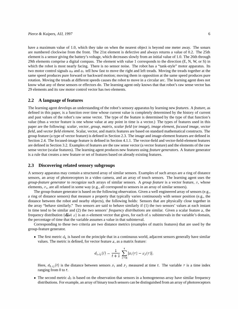
description of the sensory array with large error (unless the array really is a one-dimensional object). Using alln� 1dimensions yields a description that has zero error but contains a lot of useless information. Statisticians use a graphcalled a “scree diagram” (Figure 3a) that shows the amount of variance in the data that is accounted for by eachdimension, to subjectively choose the right number of dimensions. The image-feature generator chooses the numberof dimensions to be equal tom wherem maximizes the expression�2(m)� �2(m+ 1) where�2(m) is the variancein the data accounted for by themth dimension. For the example,m = 2. The set of two-dimensional positions foundby metric scaling for the group of distance sensors is shown in Figure 3b.
0
0.5
1
1.5
2
2.5
3
3.5
1 2 3 4 5 6 7 8 9 10
Metric scaling eigenvalues
0123
45
678910
111213141516
171819 21 22
230123
45
678910
111213141516
171819 2122
23
a b c
Figure 3:Learning a structural model of a ring of distance sensors. (a) The scree diagram gives the amount of variance (verticalaxis) accounted for by each dimension (horizontal axis) and shows that the first two dimensions account for most of the variance.(b) Metric scaling is used to assign positions to elements of the group of distance sensors. The 22-dimensional position vectors areprojected onto the first two dimensions to produce the representation shown above. (c) A relaxation algorithm is used to find a setof two-dimensional positions for the group of distance sensors that best satisfies the constraintskpi�pjk = dij : (The usefulness ofthe relaxation algorithm is more obvious in the example of the next section.) Notice the gap corresponding to the defective distancesensor. The element with index 0 corresponds to the robot’s forward sensor.
The set of(n�1)-dimensional position vectors optimally describe the structure of a group, but when these positionsare projected onto a subspace of lower dimensionality, the resulting description is no longer optimal. Elements thatwere the right distance apart inn� 1 dimensions are generally too close together in the two-dimensional projection.To compensate for this, a relaxation algorithm is used to find the best set of positions in a small-dimension space toapproximate the given distances inn�1 dimensions.The relaxation algorithm is an iterative process. On each iteration,
6The metric can be represented as a symmetric matrix with zeros on the diagonal. Such a matrix hasn(n� 1)=2 free parameters.7It seems plausible that metric scaling could be implemented using a neural net analogous to that used to implement principal component
analysis (Oja, 1982) since in both cases the main computation is the decomposition of an input matrix into a set of eigenvectors.
Pierce & Kuipers, AIJ, 1997 10
each position vector is adjusted slightly in a direction that reduces the value of the error term E (defined above). Theprocess continues until the error is very small or ceases to decrease appreciably on each iteration.8
The relaxation algorithm could be used without metric scaling by simply initializing the vector of positions ran-domly. Metric scaling provides two benefits. It shows how many dimensions are needed for the image feature, andit provides a starting point for the relaxation algorithm, decreasing the chance that the algorithm finds a local but notglobal minimum of the error function. The application of the relaxation algorithm to the group of distance sensors isillustrated in Figure 3c.
To summarize, the image-feature generator takes a group featurex and produces an image featurey whose positionvectorspi are found using metric scaling and a relaxation algorithm so that they approximately satisfy the constraints
kpi � pjk = kXt
jxi(t)� xj(t)j
while keeping the dimensionality of the position vectorspi small. The result of the experiment is a structural descrip-tion of the robot’s ring of distance sensors (Figure 3c) that is used later to analyze the robot’s motor apparatus.
2.5 Learning a sensory model of the roving eye
The learning methods are further demonstrated using a more fanciful robot called a “roving eye.” Its primary sensoryarray is a retina of photoreceptors.
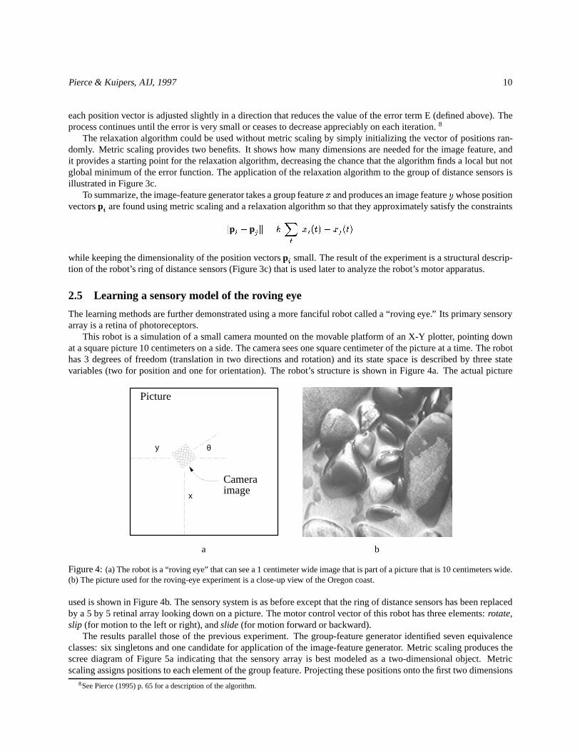
This robot is a simulation of a small camera mounted on the movable platform of an X-Y plotter, pointing downat a square picture 10 centimeters on a side. The camera sees one square centimeter of the picture at a time. The robothas 3 degrees of freedom (translation in two directions and rotation) and its state space is described by three statevariables (two for position and one for orientation). The robot’s structure is shown in Figure 4a. The actual picture
x
y θ
Picture
Cameraimage
a b
Figure 4:(a) The robot is a “roving eye” that can see a 1 centimeter wide image that is part of a picture that is 10 centimeters wide.(b) The picture used for the roving-eye experiment is a close-up view of the Oregon coast.
used is shown in Figure 4b. The sensory system is as before except that the ring of distance sensors has been replacedby a 5 by 5 retinal array looking down on a picture. The motor control vector of this robot has three elements:rotate,slip (for motion to the left or right), andslide(for motion forward or backward).
The results parallel those of the previous experiment. The group-feature generator identified seven equivalenceclasses: six singletons and one candidate for application of the image-feature generator. Metric scaling produces thescree diagram of Figure 5a indicating that the sensory array is best modeled as a two-dimensional object. Metricscaling assigns positions to each element of the group feature. Projecting these positions onto the first two dimensions
8See Pierce (1995) p. 65 for a description of the algorithm.

Pierce & Kuipers, AIJ, 1997 11
00.20.40.60.81
1.21.41.61.8
1 2 3 4 5 6 7 8 9 10
Metric scaling eigenvalues
01234
56789
1011121314
1516171819
2021222324
01234
56789
10111213
14
15161718
19
2021222324
a b c
Figure 5: (a) The metric-scaling scree diagram for the group of photoreceptors indicates that the sensors are organized in atwo-dimensional array. (b) The 2-D projection of the set of positions produced by metric scaling for the group of photoreceptorsprovides an initial approximation of the grid structure of the array of photoreceptors. (c) The final set of positions are producedusing the constraint-satisfaction relaxation algorithm, with the previous set of positions as initial values.
produces the mapping shown in Figure 5b. The set of positions produced by metric scaling is improved by therelaxation algorithm so that the distances in the resulting image more closely match the distance metricd1. Theresulting set of positions is shown in Figure 5c.
3 Learning a model of the motor apparatus
Using its learned model of the robot’s sensory system, the learning agent’s second step is to learn a model of therobot’s motor apparatus. The result of the learning is a new abstract interface to the robot that identifies the types ofmotion that the robot’s motor apparatus is capable of producing and that tells how to produce each type of motion.The source of information for this step is the sequence of values of a learnedmotion feature(a type of field feature,defined in Section 3.2) as the agent wanders by choosing motor control vectors randomly. In the simulations, if therobot is touching a wall, it is capable of turning but cannot change its position unless it is facing away from the wall.9
The image feature makes it possible to define spatial attributes of the sensory input, in terms of the locations ofsensors in the image. With spatial attributes, it is possible to define spatial as well as temporal derivatives, so motionfeatures can be defined, even without knowledge of the physical structure of the environment. The learning agent usesthe new motion feature to analyze its motor apparatus using the following steps:
1. Sample the space of motor control vectors.The robot’s infinite space of motor control vectors is discretizedinto a finite set of representative vectors,fuig.
2. Compute average motion vector fields(amvf’s). The agent repeatedly executes each representative controlvector many times in different locations and measures the average value of the resulting motion feature. It isthis average value that characterizes the effect of that control vector.
3. Apply principal component analysis (PCA).The set of computedamvf’s is a representation of the effects thatthe motor apparatus is capable of producing. PCA is used to decompose this set into a basis set ofprincipaleigenvectors, a set of representativeamvf’s from which allamvf’s may be produced by linear combination.
4. Identify primitive actions. Each principal eigenvector is matched against theamvf’s produced by the repre-sentative control vectors to find a control vector that produces that effect or its opposite. Such a motor controlvector, if it exists, is identified as aprimitive actionand can be used to produce motion for one of the robot’sdegrees of freedom.
9The use of a physical robot would require a provision such as an innate obstacle-avoidance behavior to prevent the robot from damaging itself.
Pierce & Kuipers, AIJ, 1997 12
5. Define a new abstract interface.For each degree of freedom, a new control signal is defined that allows theagent to specify the amount of motion for that degree of freedom.
The result of the learning is a new abstract interface to the robot comprised of a new set of control signals, one perdegree of freedom of the robot. The new interface hides the details of the motor apparatus. For example, whethera mobile robot’s motor apparatus uses tank-style treads or a synchro-drive mechanism, the learned interface presentsthe agent with two control signals: one for rotating and one for advancing. These learned control signals are used tofurther characterize the robot’s motor apparatus using thestaticanddynamic action models(Sections 4 and 5). Steps1 through 5 are explained in detail in the rest of this section.
3.1 Sample the space of motor control vectors
The choice of the set of representative motor control vectors must satisfy two criteria: first, they must adequately coverthe space of possiblemotor control vectorsso that the space of possibleeffects(amvf’s) is adequately represented.Second, the distribution of motor control vectors must be dense enough so that, given a desired effect (e.g., anamvfthat corresponds to one of the robot’s degrees of freedom), a motor control vector that produces that effect can befound.
Since we have already made the assumption that the motor apparatus is approximately linear, it suffices to char-acterize the effects of a uniformly distributed set of unit motor control vectors. (A unit vector has a magnitude of 1where its magnitude is equal to the square root of the sum of squares of its elements.) For two- and three-dimensionalspaces of motor control vectors, respectively, 32 and 100 vectors have been found to be adequate. For the 2-D case,it is easy to find a set of vectors that are uniformly distributed on the unit circle. Theith of n vectors has value(cos(2�i=n); sin(2�i=n)): For the 3-D case, a set of vectors uniformly distributed on the unit sphere is found usingthe relaxation algorithm of Section 2.4. The vectors are constrained to lie on the unit sphere (i.e., to have magnitude1), and the target distance between any pair of points is much larger than 2. The resulting configuration of vectorsis analogous to a collection of electrons on a charged sphere — each vector is as far from its neighbors as possible.These vectors are used as the representative motor control vectors for sampling the continuous space of average motionvector fields. This method generalizes to any dimension.
3.2 Compute average motion vector fields
A vector fieldfeature is a function over time, completely determined by the current and past values of the raw sensevector, whose value at any given time is avector field. A field is an ordered list ofvector field elements. A vectorfield element is a vector with an associated position vector. Given image featurex, (motion x) denotes a vector-fieldfeature (specifically, amotionvector-field feature) whose elements measure the amount of motion detected at thecorresponding points in the image.
To understand what this feature is measuring, suppose that, corresponding to an object in the robot’s environment,there is a property of the image feature (e.g., a local minimum or discontinuity) that changes location from one imageelement to another on subsequent time steps due to the motion of the robot. A vector from the position of the firstimage element to the position of the second represents the motion of that object and is an example of alocal motionvector. A list of local motion vectors, one for each image element, is amotion vector field.
The detection of these motion vectors does not require sophisticated object recognition. It simply requires spatialand temporal information, both of which are provided by an image feature. The spatial information is provided by thepositions of the elements of the image; the temporal information is provided by the derivatives of the elements’ valueswith respect to time. A temporal sequence of images, represented as vectors of values and associated positions, can beviewed as an intensity functionE(p; t) that maps image positions to values, called intensities, as a function of time.Such a function has both a spatial derivative,Ep and a temporal derivative,Et. The spatial derivativeEp, also calledthegradientof E, is a vector in image-position coordinates that gives the direction in which the intensity increasesmost rapidly.
A large gradient in an image detected by a robot’s sensory array corresponds to a detectable property of theenvironment such as the edge of an object. If the object moves relative to a robot’s sensory array (or vice versa), theedges detected in the image will move. This motion results in a change in intensity. A point in the image with a large

Pierce & Kuipers, AIJ, 1997 13
gradient will, in the presence of motion, also have a large temporal derivative. This is an informal motivation for theoptical flowconstraint equation [Horn, 1986], which defines the optical flow at a point in an image to have magnitude�Et=kEpk and directionEp:
v = �Et
kEpk
EpkEpk
= �EtEpkEpk2
Here,kEpk is the magnitude of the vectorEp, equal to the square root of the sum of squares of the elements ofEp.A problem with this formulation is that if the magnitude ofEp is small (or zero), then the calculation is prone toerror (or is undefined). Since the goal here is to measure average motion over time and since the measurement of theoptical flow is more precise at edges or, in general, when the gradientEp is large, we have found it useful to weightthe expression using the termkEpk2 and measure the value of:
v = �EtEp
In most computer vision applications, images are represented as regularly spaced arrays of pixels (picture ele-ments). With such a representation, it is straightforward to define an approximation for the spatial derivative at a pointin the image. The images as defined here, however, do not have such a regular structure so we use a different approachto defining what we call thesensory flow field. The sensory flow measured at elementi is taken to be a weighted sumof local motion vectorsvij in the direction from elementi to elementj wherej ranges over all of the elements closeto elementi (as defined in Section 2.3). The weight is inversely proportional to the distance between elementsi andj.The precise definition of themotion operator is given below, where(posx) denotes the vector of positions associatedwith featurex, and(val x) denotes the vector of values associated with featurex.
pos(motion x)def= posx
(val(motion x))idef=
Xj�i
vij=kpijk
pij = (posxj)� (posxi)
vij = �Et;iEp;ij
Et;i =d
dt(val x)i
Ep;ij =((val x)j � (val x)i)
kpijk
pij
kpijk
Here,kpijk is the distance in the image between the positions of elementsi andj; Et;i is the temporal derivative ofthe intensity function for elementi; andEp;ij is the component of gradientEp at elementi in the direction towardelementj.
Using themotion operator, the definition of theamvf associated with theith representative motor control vectorui is
amvfi = � ((motion x) j (= u ui))
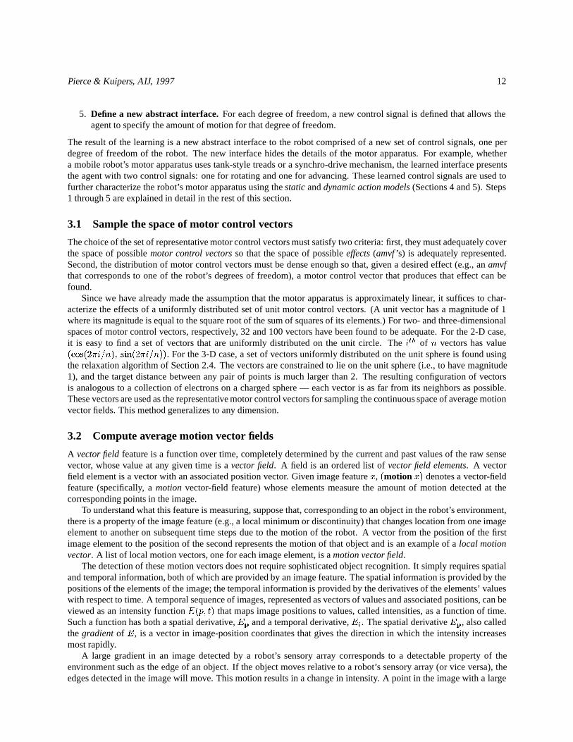
wherex is the image feature that has already been learned (Section 2.4),u is the motor control vector used to controlthe motor apparatus, and� is an operator that computes the average value of its argument. In this case, the averagevalue is taken over all time steps during whichui was taken. Examples are shown in Figure 6. These are obtained afterthe learning agent has wandered for 20 minutes using the exploration strategy of randomly choosing a representativemotor control vector and executing it for one second (ten time steps).
3.3 Apply principal component analysis
The goal of this step is to find a basis set for the space of effects of the motor apparatus, i.e., a set of representativemotion vector fields from which all of the motion vector fields may be produced by linear combination. This type ofdecomposition may be performed using principal component analysis (PCA). (See Mardia et al. [Mardia et al., 1979]
Pierce & Kuipers, AIJ, 1997 14
(1.00 -0.01) (0.74 0.68) (-0.05 1.00) (-0.72 0.69)
(-1.00 0.01) (-0.74 -0.68) (0.05 -1.00) (0.72 -0.69)
Figure 6:Examples of average motion vector fields (amvf’s) (represented as collections of line segments) and associated motorcontrol vectors (shown in the lower-left corner of each picture). Anamvf associates an average local motion vector with eachposition in an image (see Figure 3). Each line segment represents the position, direction, and magnitude of one of these averagelocal motion vectors.
for an introduction. Oja [Oja, 1982] discusses how a neural network can function as a Principal Component Analyzer.Ritter et al. [Ritter et al., 1992] show that self-organizing maps [Kohonen, 1988] can be seen as a generalization ofPCA.)
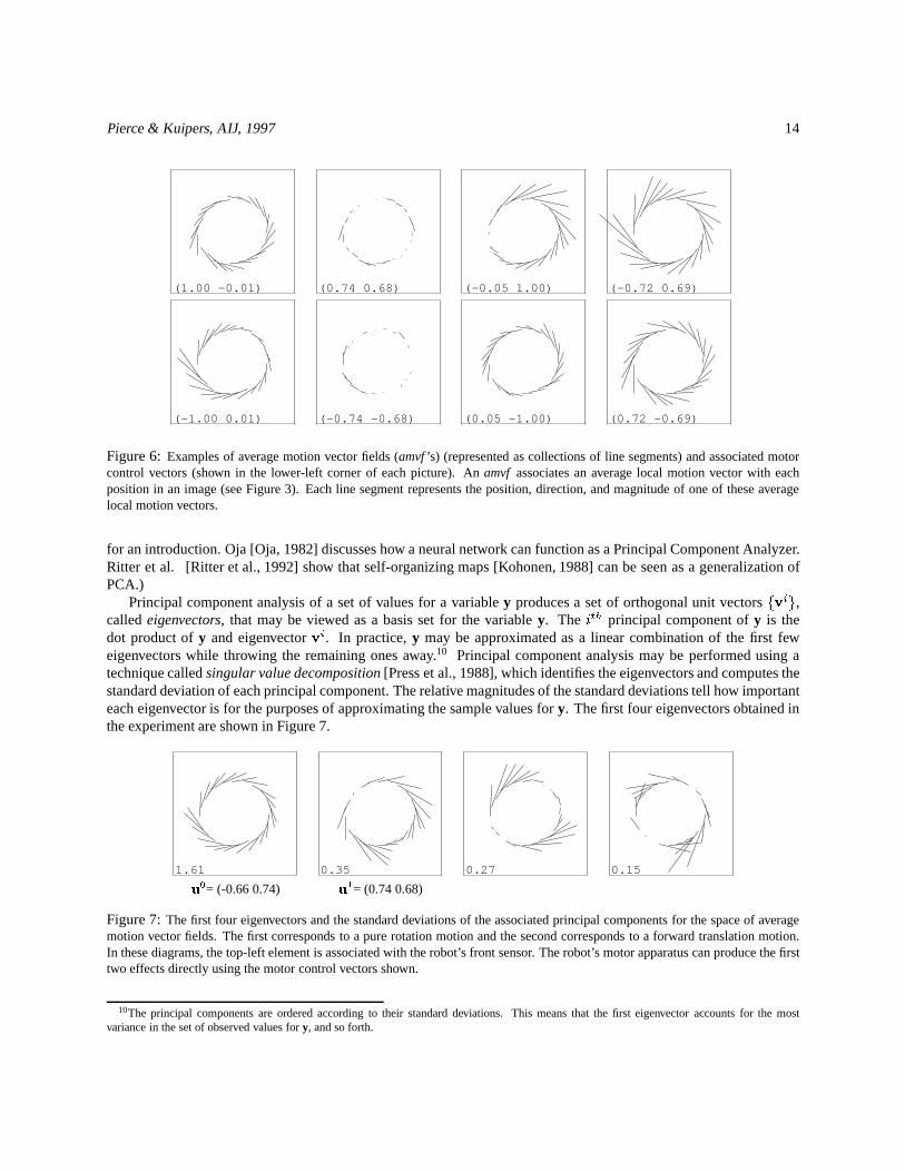
Principal component analysis of a set of values for a variabley produces a set of orthogonal unit vectorsfvig,calledeigenvectors, that may be viewed as a basis set for the variabley. The ith principal component ofy is thedot product ofy and eigenvectorvi. In practice,y may be approximated as a linear combination of the first feweigenvectors while throwing the remaining ones away.10 Principal component analysis may be performed using atechnique calledsingular value decomposition[Press et al., 1988], which identifies the eigenvectors and computes thestandard deviation of each principal component. The relative magnitudes of the standard deviations tell how importanteach eigenvector is for the purposes of approximating the sample values fory. The first four eigenvectors obtained inthe experiment are shown in Figure 7.
1.61 0.35 0.27 0.15
u0= (-0.66 0.74) u
1= (0.74 0.68)
Figure 7:The first four eigenvectors and the standard deviations of the associated principal components for the space of averagemotion vector fields. The first corresponds to a pure rotation motion and the second corresponds to a forward translation motion.In these diagrams, the top-left element is associated with the robot’s front sensor. The robot’s motor apparatus can produce the firsttwo effects directly using the motor control vectors shown.
10The principal components are ordered according to their standard deviations. This means that the first eigenvector accounts for the mostvariance in the set of observed values fory, and so forth.

Pierce & Kuipers, AIJ, 1997 15
3.4 Identify primitive actions
In the previous step, principal component analysis was used to determine a basis set of effects for the motor apparatus,namely, the set of eigenvectors. The goal of this step is to discover which motor control vectors can be used toproduce those effects. This is accomplished by matching the eigenvectors with theamvf’s of all of the representativemotor control vectors. The matching involves computing, for eachi andj, the angle�ij between theith eigenvectorand thejth amvf. This angle is defined by the equation�ij = vi � amvfj where the vector fieldsvi andamvfj aretreated as simple vectors by flattening theirnm-dimensional local motion vectors into a singlenm-dimensional vectorand ignoring the positions of the local motion vectors. An angle near zero indicates that theamvf is similar to theeigenvector. An angle near 180 degrees indicates that theamvf is similar to the opposite of the eigenvector. If anyamvf’s match theith eigenvector to within 45 degrees, then actionui+ is defined to be the motor control vector whoseamvf is most collinear with theith eigenvector andui� is defined to be the motor control vector whoseamvf is mostanti-linear.11 The definitions of control laws (Section 5) assume that the robot’s motor apparatus is linear, implyingthatui+ = �ui�. In the case thatui+ � �ui�, they can be approximated by plus and minusui, respectively, where
ui def= 1
2 (ui+ �ui�). Subsequently, this will be used as the definition of theith primitive action. The values ofui are
shown in Figure 7. The analogous results for the roving-eye experiment are shown in Figure 8.
0.43 0.37 0.21 0.04
(-0.17 -0.99 -0.05) (0.03 0.03 -1.00) (-0.99 0.13 0.04)
Figure 8:The first four principal eigenvectors and associated singular values for the roving-eye robot. The first two correspondto pure translation motions and the third corresponds to a pure rotation motion. The robot’s motor apparatus can produce the firstthree effects directly using the motor control vectors shown.
3.5 Define a new abstract interface
The goal of this step is to define a new interface to the robot that abstracts away the details of the motor apparatus.For each of the robot’s degrees of freedom, a new control signal is defined for producing motion along that degree offreedom. Negative values of the control signal move the robot in the opposite direction. For the robot of the example,there are two control signals, one for turning (left and right) and one for advancing (forward and backward). The effectof the control signals is defined by the following equation:
u = u0u0 + u1u
1
whereu0 andu1 (which range from -1 to 1) are the new control signals andu0 andu1 are the primitive actionscorresponding to the first two principal eigenvectors.
3.6 Discussion
The learning methods described in this section have also been applied to a simulated synchro-drive robot for whichthe motor control signals directly specify how fast to turn and advance, respectively. The details of that experiment aregiven in [Pierce, 1991b]. The synchro-drive and tank-style robots demonstrate two different motor apparatuses withidentical capabilities. The learned abstract interface, since it is grounded in sensory effects rather than motor control
11This matching criterion is more restrictive than it appears. In a high-dimensional space such as the space ofamvf’s, it is highly unlikely thattwo random vectors will define an angle less than 45 degrees.
Pierce & Kuipers, AIJ, 1997 16
signals, is the same for both: it abstracts away the details of the motor apparatus, providing a new set of control signals,one for each of the robot’s degrees of freedom.
The learning methods described in this section build on the sensory image structure learned in the previous section.The result is a new abstract interface whose control signals are used in Section 5 to define behaviors for navigation.
4 Local state variables
The result of the agent’s learning so far is an abstract interface that includes a model of the robot’s sensorimotorapparatus. The model of thesensoryapparatus is the description of its physical structure represented primarily by thepositions of the elements of the learned image feature. The model of themotorapparatus is the set of learned primitiveactions that tells the agent how many degrees of freedom it has, and how to produce motion in each.
The agent’s ultimate goal is to abstract the continuous world of the robot to acognitive mapby which the worldis viewed as a discrete set of recognizable places with well-defined paths connecting them. The cognitive map givesthe learning agent the ability to predict the effects of high-level behaviors and to navigate among a set of recognizableplaces. Learning the cognitive map requires that the agent learn path-following behaviors for moving the robot throughits state space. In order to be useful for prediction, these behaviors must be repeatable in the sense that executing abehavior from a given initial state always moves the robot to the same final state. The following paragraph gives a fewexamples of such path-following behaviors.
If the learning agent has a feature that gives the distance from the robot to the wall and it knows how to make therobot move while keeping this feature constant, then it can make the robot follow the wall. For a robot with a retina(Section 2.5), a feature as simple as the sum of all of the inputs could be used to define a path-following behavior.Moving while keeping the feature constant would correspond to following a path of constant intensity. A more complexfeature based on the retina is a line detector, which could be used as the basis for a line-following behavior. For a robotwith a continuous compass giving the robot’s heading, a path-following behavior based on the compass’s value wouldmove the robot in a constant direction. Finally, consider a robot with an omni-directional photo-sensor responding to alight mounted on the robot and suppose that the robot is in a dark room with white walls. The amount of light detectedby the robot’s sensor would decrease with distance from the nearest wall. A wall-following behavior could be basedon an error signal that was the difference between the light level detected by the sensor and a nominal value (e.g., avalue in the middle of the sensor’s range of values).
In this section and the next, we describe the following three-step method for learning path-following behaviors:(1) find a set of features that the learning agent can control, calledlocal state variablesand use them to define errorsignals; (2) learn behaviors for minimizing the error signals; and (3) learn behaviors that move the robot while keepingthe errors near zero. This section shows how to learn local state variables. Section 5 shows how to use them to definepath-following behaviors.
What is required of a local state variable is that it be controllable, i.e., the learning agent must know how its controlsignals affect it. A feature is controllable if it meets the following definition:
Let u be the vector of control signalsuj . A scalar featureyi is a localstate variableif the effect of the control signals onyi can be approxi-mated locally by
_yi =mi � u (=Xj
mij uj) (1)
wheremi is nonzero.
Determining whether a feature is a local state variable while learning the context-dependent value ofmi is the job ofthe static action model (Section 4.2). The source of information for this step is the set of learned features producedwhile the learning agent wanders by using its learned primitive actions.
Local state variables are analogous to state variables in the following sense. Ifx is a state variable, then theconstraint_x = 0 reduces the dimensionality of the robot’s state space by one. Ify is a local state variable, then the
Pierce & Kuipers, AIJ, 1997 17
constraint_y = 0 reduces the dimensionality of the robot’s motor control vector space by one.12 In other words, theconstraint reduces the robot’s degrees of freedom by one. Since the learning agent does not have access to the robot’sstate space, it defines local state variables using its knowledge of motor control vector space to which it does haveaccess. They are calledlocal state variables because they are not required to be defined everywhere in the robot’s statespace.
An important feature of local state variables is that they are controllable: featureyi may be moved to a target valuey�i using a simple control law. This fact is exploited in the definition of the homing behaviors (Section 5.2). Thediscovery of local state variables has two components: generating new features (Section 4.1), and testing each featureto see if it satisfies the definition of local state variable (Section 4.2).
4.1 Generating new features
If a sensory system does not directly provide useful features, it may be possible to generate features that are useful.A generate-and-test approach is demonstrated in the following experiment using the tank-style mobile robot in whichthe agent learns new scalar features that are better candidates for local state variables than are the elements of the rawsense vector.
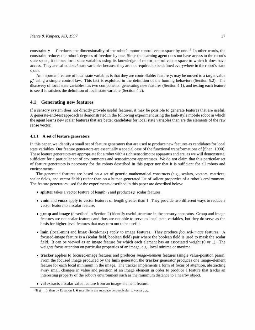
4.1.1 A set of feature generators
In this paper, we identify a small set of feature generators that are used to produce new features as candidates for localstate variables. Our feature generators are essentially a special case of the functional transformations of [Shen, 1990].These feature generators are appropriate for a robot with a rich sensorimotor apparatus and are, as we will demonstrate,sufficient for a particular set of environments and sensorimotor apparatuses. We do not claim that this particular setof feature generators is necessary for the robots described in this paper nor that it is sufficient for all robots andenvironments.
The generated features are based on a set of generic mathematical constructs (e.g., scalars, vectors, matrices,scalar fields, and vector fields) rather than on a human-generated list of salient properties of a robot’s environment.The feature generators used for the experiments described in this paper are described below:
� splitter takes a vector feature of lengthn and producesn scalar features.
� vmin andvmax apply to vector features of length greater than 1. They provide two different ways to reduce avector feature to a scalar feature.
� group andimage(described in Section 2) identify useful structure in the sensory apparatus. Group and imagefeatures are not scalar features and thus are not able to serve as local state variables, but they do serve as thebasis for higher-level features that may turn out to be useful.
� lmin (local-min) andlmax (local-max) apply to image features. They producefocused-imagefeatures. Afocused-image feature is a (scalar field, boolean field) pair where the boolean field is used to mask the scalarfield. It can be viewed as an image feature for which each element has an associated weight (0 or 1). Theweights focus attention on particular properties of an image, e.g., local minima or maxima.
� tracker applies to focused-image features and producesimage-elementfeatures (single value-position pairs).From the focused image produced by thelmin generator, thetracker generator produces one image-elementfeature for each local minimum in the image. The tracker implements a form of focus of attention, abstractingaway small changes in value and position of an image element in order to produce a feature that tracks aninteresting property of the robot’s environment such as the minimum distance to a nearby object.
� val extracts a scalar value feature from an image-element feature.12If _y = 0, then by Equation 1,u must lie in the subspace perpendicular to vectormi.

Pierce & Kuipers, AIJ, 1997 18
This set of feature generators has proven successful for the robot with a ring of distance sensors. To handle the “rovingeye” robot, we would augment this set with generators for features based on a variety of convolution masks andother two-dimensional image-processing operators. An interesting open problem is to define a general set of featuregenerators appropriate to learning mobile robots, analogous to the small and general set of functional transformationsused by Shen [Shen, 1990] to replicate the performance of AM [Lenat, 1977]. We conjecture that a reasonably sizedset of feature generators will apply to a broad class of mobile robots and that such a set of feature generators can bediscovered by developing solutions for a small subset of that class: initially, each new robot would require one or morenew feature generators; eventually the set of feature generators would converge to a generally applicable set.
4.1.2 Generating and testing features
The generate-and-test process of learning potentially useful features executes the following steps in a continuous loop.Initially, there is only one feature, theraw sensory feature. This feature is marked as new.
1. Each generator is applied to each new feature to which it is applicable.
2. The features that were new are marked as old, and the features just generated are marked as new.
In generate-and-test approaches to learning, controlling the search through a large space of possibilities is an importantconcern. Without any constraints, the number of features generated on each iteration of the generate-and-test loopmay grow exponentially. There are several ways to constrain a search algorithm. One way is to limit the depth of thesearch. In the current implementation of the generate-and-test algorithm, it is possible to set a limit on the number ofgenerations of new features that are created. A second way is to limit the breadth of the search. This method is used ingenetic algorithms where population size is constrained to a certain number. This method requires a fitness measureto tell which members of the population are worthy of survival. Such a fitness measure can be defined as a featuretester, though this has not been done here. A third way to constrain a search space is to limit the branching factor. Forthe feature-learning problem, this is the average number of new features that are generated for each old feature at eachstep of the generate-and-test process. The branching factor for the feature learning problem is limited in two ways:the total number of generators is kept reasonably small and the number of generators that apply to any given feature iskept small by using strongly typed generators (e.g., the image-feature generator only applies to group features).
4.1.3 An experiment
In the experiments described in this paper, the combinatorial explosion of features has not been an issue. The gen-erators form deep but narrow hierarchies with a tractable set of features. To study this, we devised an experiment inwhich the agent explores by randomly choosing unit motor control vectors and executing them for one second (10time steps) each. Figure 9 shows the complete hierarchy of features and generators for the learning agent’s feature-learning process. At the top of the figure is the raw sense vectors. We refer to each feature using a name derived fromthe sequence of feature generators used to produce that feature (where g=group, im=image, tr=tracker, val=value).Thus, for example,s-g-vminresults from applying thevmin generator to the feature produced by applying thegroupfeature generator to the raw sense vectors. The features shown in the figure are, from top to bottom and from leftto right: s, s-g, s-vmin, s-vmax, s0, s1, : : :, s28, s-g-im, s-g-vmin, s-g-vmax, s-g-im-lmin, s-g-im-lmax, s-g-im-lmin-tr,s-g-im-lmax-tr, s-g-im-lmin-tr-val, ands-g-im-lmax-tr-val. Notice that, depending on the robot’s position, there maybe multiples-g-im-lmin-tr-valor s-g-im-lmax-tr-valfeatures. Each of the generatedscalar features (the leaves of thetree of generated features) is tested (Section 4.2) to see if it can serve as a local state variable.
4.2 The static action model
The purpose of the static action model (a set of equations of the form given in Equation 1 of Section 4) is to predict thebehavior of each scalar feature. The learning of the static action model for a feature proceeds in three steps. In the firststep, the learning agent tries to predict the behavior of the feature without taking into account which primitive actionis being used. If it fails, then it tries to predict the behavior of the feature as a function of the action being taken. Ifthis fails for a primitive action, then the agent tries to predict the context-dependent effect of that action on the feature.

Pierce & Kuipers, AIJ, 1997 19
vector
group
image
scalar
tracker
lmin lmax
group
image
tracker
vmin, vmax
scalar
value
focused image
imageelement
splittervminvmax
Figure 9: The complete hierarchy of features and generators in the learning agent’s feature-learning process used to producecandidate local state variables. The feature generators are shown in bold face; the feature types are shown in italics.

Pierce & Kuipers, AIJ, 1997 20
If a feature is action dependent and is predictable in all contexts, then it can serve as a local state variable.13 With theinformation contained in the static action model, it is a simple matter to define homing behaviors for moving the robotso that the local state variable moves toward a target value.
When trying to predict the effects of actions on features, the learning agent looks for approximately linear rela-tionships between action magnitudes and feature derivatives because the control laws used to define path-followingbehaviors (Section 5) are based on the assumption that these relationships are approximately linear.
4.2.1 An action-independent model
The first step toward modeling the behavior of a featureyi is to see if it is possible to predict its behavior independentlyof the motor control vector being used. The agent explores by repeatedly choosing a primitive action and executing itfor one second (ten time steps). It analyzes the behavior of the feature using a device that we call acorrelator. Thisproduces a set of statistics based on the plot of the feature’s value as a function of time (Figure 10). The coordinate for
�s0 vs.�t �s24 vs.�t lmin vs.�t
Figure 10:Plots of�yi (vertical axis) vs.�t (horizontal axis), used by the learning agent to try to predict the behavior of featureyi independently of the motor control vector. Whenever a new motor control vector is used,�yi and�t are reset to 0 (at thecenter of each plot). From the sets of(�t;�yi) points, statisticsmi, ri, and i are computed (see text). The numbers shown arethe correlationsri between�yi and�t. From these statistics the learning agent concludes that featuress0 and lmin (short fors-g-im-lmin-tr-val) are unpredictable ( is large andr is small) and thats24 is constant ( < 0:001).
the horizontal axis is�t = t � t0 wheret0 is the last time the motor control vector changed. The vertical axis gives�yi = yi(t)� yi(t0).
The statistics aremi, ri, and i. The value ofmi is the slope of the line that best fits the set of(�t;�yi) points.The value ofri is the correlation between variables�yi and�t. The value of i is the ratio of the standard deviationsof �yi and�t. It is a measure of how fast the feature changes as a function of time. A number of properties aredefined in terms of these statistics. The feature isconstant if i < 0:001. It is increasing if ri > 0:6; decreasingifri < �0:6. It is predictable if any of these properties holds. Otherwise, it is unpredictable and the learning agent triesto predict the behavior of the feature using an action-dependent model.
For the running example, the featuress-vmin, s-vmax, s20 (the broken distance sensor),s24 (the battery voltage),ands-g-vmaxare all diagnosed asconstant and are thus not suitable for use as local state variables. The rest arecandidates for the next step in the learning of the static action model.
4.2.2 An action-dependent model
If the previous step failed to produce a model that predicts the behavior of a featureyi, then the learning agent usesone correlator for each primitive action to analyze its effect on the feature. In this case, the correlator characterizesthe relationship betweenuj�t and�yi where�t and�yi are defined as before. The agent continues to explore byrandomly selecting primitive actions and executing them for a second at a time. It computes the statisticsmij (the slope
13One could use a less constrained definition of local state variable: if a feature is action dependent and predictable in a given context, then it is alocal state variable for that context. We have chosen the more constraining definition because it results in more robust control laws.

Pierce & Kuipers, AIJ, 1997 21
of the line that best fits the set of(uj�t;�yi) points),rij (the correlation betweenuj�t and�yi), and ij (the ratioof the standard deviations ofuj�t and�yi). A feature is labeledconstant for control signaluj if ij < i=4. Thepropertiesincreasing, decreasing, andpredictable for control signaluj are defined as before. For each predictablefeature-control signal pair, a rule of the form
_yi = mij uj
is added to the static action model. If a feature is predictable for all of the primitive actions, then the feature itself is
�s0 vs. u0�t �s0 vs.u1�t �lmin vs.u0�t �lmin vs. u1�t
Figure 11:Plots of�yi vs.uj�t for two features and two primitive actions. These are used to see if it is possible to predict thebehavior of the feature as a function of the motor control vector. Features0 is unpredictable for actionu0 (r is small and is large)but predictable for actionu1 (r is large). Featurelmin is constant for actionu0 ( < 0:001) but unpredictable for actionu1 (r issmall and is large).
predictable.For the running example (Figure 11), all of the distance sensors are found to be unpredictable for primitive action
u0 (rotating). The effect ofu1 (advancing) is to decrease featuress0, s1, s2, s3, ands23; to increase featuress9 throughs14. Its effect is unpredictable for featuress4–s8, s15–s19, s21, ands22. The discrete compass sensorss25 throughs28are unpredictable foru0 and constant foru1. The featuress-g-vminands-g-im-lmin-tr-val(a.k.a.lmin) are constantfor u0 and unpredictable foru1. Features-g-im-lmax-tr-val(a.k.a.lmax) is unpredictable for both primitive actions.One might guess thatlmaxwould be constant foru0. In fact,lmax, which is only defined when the robot is in a corner,fluctuates too rapidly with small turns to be diagnosed as constant.
4.2.3 A context-dependent model
If uj has an effect onyi that is unpredictable, then the learning agent tries to find a partition of sensory space into adiscrete set of contexts so that the relationship can be approximated by a linear equation for each context.14 In general,a context featurezij , for local state variableyi and control signaluj , is an integer-valued feature that takes on a finiteset of values. This set defines a partition of the robot’s state space into a finite set of contexts defined by the predicateszij = k. One way to define a context feature is to first choose a featurex and divide its range of values into a finiteset of intervals,fIkg, where each interval defines its own context. The context feature is then defined byzij = k iffx 2 Ik . Using featurex to define a set of contexts is appropriate if the value ofx is a good predictor of the effect ofthe control signaluj on the featureyi. To test the hypothesis thatx is a good predictor for the effect ofuj on yi, acorrelator can be used to determineuj ’s effect onyi for each context defined by the predicatezij = k.
Testing each of a large set of features to see if they improve the predictability of a control signal’s effect is ex-pensive. Heuristics can be used to guide the search for relevant features to use in defining contexts. For example, itmakes sense to first look at features that are closely related to the feature being analyzed, in the sense that they areclose together in the tree of features produced by the generate-and-test process.
Currently, only one such heuristic is implemented: if a feature is based on the value of a element of an image, thenuse the position of that element in the image to define the context. Since there is a discrete set of possible positionsfor an image-element feature, it is trivial to break the space of possible positions into a discrete set of contexts. For
14This approach is analogous to Drescher’s marginal attribution [Drescher, 1991].

Pierce & Kuipers, AIJ, 1997 22
example, in the case of thelmin and lmax features, there are 23 possible positions and these can be used to breaksensory space into a partition of 23 contexts each defined by the predicatezij = k wherezij is an integer featurewhose value is between 0 and 22 and identifies the position associated with the local minimum or maximum.
For each contextzij = k, a correlator is used to try to predict the effect ofuj onyi given that the robot is in thatcontext. The agent continues to explore randomly while computing the statisticsmijk , rijk , and ijk . The propertiesconstant, increasing, decreasing, andpredictable are defined as before. For each predictable context, a rule of theform
_yi = mijk uj , if zij = k
is added to the static action model. Ifmijk is 0, then the predicatezij = k defines a “constant context” (which isuseful for defining path-following behaviors). If the primitive action’s effect on the feature is predictable for everycontext, then the feature is predictable for that action.
For the running example, the only features with associated context features arelmin andlmax.
� lmin is already predictable (constant) for control signalu0.
� The effect ofu1 on lmin is predictable for every context. Its effect is to decreaselmin for contexts 0–5 and19–22, and to increase it for contexts 7–17. For contexts 6 and 18 (in which the robot’s heading is parallel to thewall), lmin is constant (see Figure 12).
� The effect ofu0 on lmax is unpredictable for almost every context.
� The effect ofu1 is to decreaselmax for contexts 0–5 and 20–22 and to increase it for contexts 8–16. The effectis unpredictable for contexts 6, 7, 17, and 18.
k=0 k=6 k=12
Figure 12:Example plots of�yi vs.u1�t for thes-g-im-lmin-tr-valfeature for three different contexts. These are used to see ifit is possible to predict the behavior of the feature as a function of the motor control vector and the current context. For actionu1,featurelmin is decreasing, constant, andincreasingfor contexts 0, 6, and 12, respectively.
At this point the only feature that is both predictable and action-dependent (and is thus a local state variable) islmin.Its behavior can be modeled by the equation_yi = mi1k u1 wherek is the current value of the context featurezij thatrepresents the location of the local minimum in the image feature. The featurelmin was produced by thetrackergenerator. This generator actually produces multiplelmin features, one for each local minimum in the input imagefeature. The number of local state variables depends on the robot’s location. There are two local state variables in theneighborhood of a corner, three in the neighborhood of a T-intersection, but just one if only a single wall is withinrange.
5 Learning control laws
The goal of this step is to learn a suitable set ofhomingandpath-following behaviorsusing the results of the precedingsections, specifically, the set of local state variables and the set of primitive actions. Recall that for the robot of the

Pierce & Kuipers, AIJ, 1997 23
running experiment, the local state variables are thelmin features, the only features identified as controllable by thelearning agent. The sources of information for this step are the learned static action model (Section 4.2) and dynamicaction model (Section 5.3.2).
A behavior, as the term is used in this paper, is an object with four components, calledoutput, app, done, andinit. The outputcomponent is a function that returns a vector of motor control signals. Theapp component is ascalar function whose value indicates whether the behavior is currently applicable. The value of this feature may be0 (indicating that the behavior is not applicable) or 1 (indicating that the behavior is applicable) or some number inbetween (indicating a certainty less than 100% that the behavior is applicable). Thedonesignal is a Boolean functionthat tells when the behavior has finished. Theinit signal is an input signal that tells the behavior to initialize itself (incase it has internal state information that needs to be reset).
Path-following behaviors are learned in three steps: (1) continuous error signals are defined; (2) behaviors arelearned for minimizing the error signals; (3) behaviors are learned for moving while keeping the error signals nearzero.
5.1 Defining error signals for control laws
The learning agent’s approach to exploration, mapping, and navigation uses path-following behaviors in which therobot moves while maintaining an error signal near zero. An example of a path-following behavior based on an errorsignal involves a person walking down a corridor. The error signal ise = (y� � y) wherey is the distance from theperson to the right side of the corridor (left in Britain) andy� is a constant that depends on the person, his mood, andthe number of other people in the corridor. The error signal is used in a control law for moving along the corridor.If the error is positive, the person moves to the left (away from the wall) while walking; if it is negative, he movesto the right. The control law is efficient and repeatable: by using the control law, the person follows an efficient (i.e.,straight) path from one end of the corridor to the other, and each time the person follows the path, he ends up in thesame place.
In this example,y is a local state variable. The agent’s approach to defining path-following behaviors is to firstdefine error signals of the forme = y� � y for each local state variabley.15
5.2 Learning homing behaviors
The purpose of ahoming behavioris to move an error signal toward zero so that path-following behaviors based onthat error signal will become applicable. While it would be possible to use reinforcement-learning methods to learn ahoming behavior given an error signal [Pierce and Kuipers, 1991, Lin and Hanson, 1993], most of the relevant learninghas already been done. The homing behavior can be defined as an instance of the generic, domain-independent controllaw in Figure 13, drawing on the knowledge in the static action model.
For each local state variableyi and control signaluj , a homing behavior is defined for reducing the errore =y�i � yi. It is applicable in every contextzij = k for which the static action model includes a rule of the form_yi = mijkuj wheremijk is nonzero. It is done when the error is close to zero. Its output is given by a simple controllaw. The definition is based on the partition of sensory space used by the static action model to characterize the effectsof uj on yi. This partition is described by the set of contextsfkg. The components of the homing behavior (app,output, anddone) are defined for each possible contextk (Figure 13). A homing behavior that the agent learns for themobile robot is illustrated in Figure 14.
5.3 Learning path-following behaviors
The previous section presented a method for learning homing behaviors that minimize a given error signal. In thissection, a method is presented for moving while minimizing the error signal. The result is a path-following behavior.Learning a path-following behavior involves two steps: 1) learning how to move in the general direction that keeps the
15Choosing an optimal target valuey� for a featurey is beyond the scope of this paper. The implemented learning agent chooses a value equalto half the feature’s maximum value.
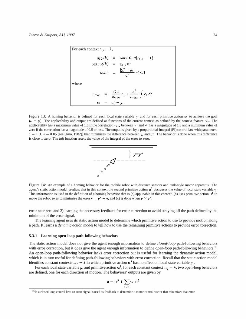
Pierce & Kuipers, AIJ, 1997 24
For each contextzij = k,
app(k) = maxf0; 2jrijk j � 1g
output(k) = uijk uj
done �jy�i � yij
y�i< 0:1
where
uijk =2�!
mijk
ei +!2
mijk
Zei dt
ei = y�i � yi:
Figure 13: A homing behavior is defined for each local state variableyi and for each primitive actionuj to achieve the goalyi = y�i . The applicability and output are defined as functions of the current context as defined by the context featurezij . Theapplicability has a maximum value of 1.0 if the correlationrijk betweenuj and _yi has a magnitude of 1.0 and a minimum value ofzero if the correlation has a magnitude of 0.5 or less. The output is given by a proportional-integral (PI) control law with parameters� = 1:0, ! = 0:05 (see [Kuo, 1982]) that minimizes the difference betweenyi andy�i . The behavior is done when this differenceis close to zero. Theinit function resets the value of the integral of the error to zero.
y=y*
Figure 14:An example of a homing behavior for the mobile robot with distance sensors and tank-style motor apparatus. Theagent’s static action model predicts that in this context the second primitive actionu
1 decreases the value of local state variabley.This information is used in the definition of a homing behavior that is (a) applicable in this context, (b) uses primitive actionu
1 tomove the robot so as to minimize the errore = y� � y, and (c) is done wheny � y�.
error near zero and 2) learning the necessary feedback for error correction to avoid straying off the path defined by theminimum of the error signal.
The learning agent uses its static action model to determine which primitive action to use to provide motion alonga path. It learns adynamic action modelto tell how to use the remaining primitive actions to provide error correction.
5.3.1 Learning open-loop path-following behaviors
The static action model does not give the agent enough information to defineclosed-looppath-following behaviorswith error correction, but it does give the agent enough information to defineopen-looppath-following behaviors.16
An open-loop path-following behavior lacks error correction but is useful for learning the dynamic action model,which is in turn useful for defining path-following behaviors with error correction. Recall that the static action modelidentifies constant contextszij = k in which primitive actionuj has no effect on local state variableyi.
For each local state variableyi and primitive actionuj , for each constant contextzij = k, two open-loop behaviorsare defined, one for each direction of motion. The behaviors’ outputs are given by
u = u� +XÆ 6=j
uÆ uÆ
16In a closed-loop control law, an error signal is used as feedback to determine a motor control vector that minimizes that error.

Pierce & Kuipers, AIJ, 1997 25
whereu� = �uj andjuÆj � 1. TheuÆ components are used in learning the dynamic action model. The purpose ofan open-loop path-following behavior is to allow the agent to learn the effects of theorthogonalcontrol signals on thefeature while motor control vectoru� is used.17 With this knowledge, it is possible to use the other control signalsfor error correction. The definition of open-loop path-following behaviors is summarized in Figure 15. A behavior is
app �jy�i � yij
y�i< 0:1 ^ zij = k
output = u� +XÆ 6=j
uÆuÆ
done �jy�i � yij
y�i> 0:4
_ (a new behavior becomes applicable)
Figure 15:An open-loop path-following behavior is defined for each local state variableyi, for each primitive action (or opposite)u� , and for each constant contextzij = k. The predicatezij = k defines a constant context if it implies thatu� maintainsyi
constant according to the static action model. The behavior is applicable when the error signaly�i � yi is small. The output hastwo components: a base motor control vector and a small orthogonal component. During learning of the dynamic action model, theorthogonal component changes every 3 seconds. Only one of theuÆ ’s is nonzero at a time. The behavior is done when the errorsignal is too large or a new behavior becomes applicable.
done when the robot strays too far off the path or when a new behavior becomes applicable indicating that the agenthas a choice to make: to continue the current behavior or start a new one.
For the mobile robot of the running example, there is an open-loop path-following behavior based onu0 (forturning) for each local state variableyi (see Figure 16a). It is applicable wheneveryi = y�i since, according to the
y=y*
(a) (b)
Figure 16:Two examples of open-loop path-following behaviors. (a) A behavior based onu0 (for turning) and constraintyi = y�i
is applicable wheneveryi = y�i sinceu0 never changes the value ofyi. (b) A behavior based on primitive actionu1 (advancing)and constraintyi = y�i is applicable wheneveryi = y�i and the robot’s heading is parallel to the wall on its left (i.e.,zij = 18)since in this contextu1 keeps the errore = y�i � yi near zero.
static action model, turning has no effect onyi. There is also an open-loop path-following behavior based onu1
(for advancing) for each featureyi (see Figure 16b). It is applicable when the robot is facing parallel to the objectbeing detected byyi (that is, when context featurezij has value 6 or 18). Figure 20b shows a trace of the behavior ofthe robot that results as the learning agent uses its learned open-loop path-following behaviors to explore the robot’senvironment.
5.3.2 The dynamic action model
The static action model predicts the context-dependent effects of a control signal on the local state variables. Thedynamicaction model predicts the context-dependent effects of control signals on the local state variables while anopen-loop path-following behavior is being executed.
17The primitive actions are orthogonal to each other in the sense that theiramvf’s are orthogonal to each other (see Section 3.3).

Pierce & Kuipers, AIJ, 1997 26
The dynamic action model tells, for each open-loop path-following behavior, the effect of each orthogonal action(each primitive action other than the path-following behavior’s base action), on the local state variable that is usedin the definition of the path-following behavior’s error signal. To learn the dynamic action model, an explorationbehavior is used that randomly chooses applicable homing and open-loop path-following behaviors. A behavior runsuntil it is no longer applicable, or a new path-following behavior becomes applicable. Linear regression is used tolearn the relationships between the orthogonal actionsuÆ and the featuresyi in the context of running the open-looppath-following behavior based on featureyi, motor control vectoru� = �uj , and contextzij = k. While it is running,linear regressors test the hypotheses_yi = mijkÆ1 uÆ and�yi = mijkÆ2 uÆ by computing the correlationsrijkÆn between
uÆ andy(n)i . If rijkÆ1 > rijkÆ2 andjrijkÆ1 j > 0:6, then the rule
_yi = mijkÆ1 uÆ; if zij = k ^ u = �uj + uÆuÆ
is added to the dynamic action model. Otherwise, ifjrijkÆ2 j > 0:6, then the rule
�yi = mijkÆ2 uÆ if zij = k ^ u = �uj + uÆuÆ
is added to the dynamic action model. Otherwise, the relationship betweenuÆ andyi is either zero or unpredictable.18
Suppose that the mobile robot of the running experiment has a wall to its left and that its heading is parallel tothe wall (Figure 16b). In this context, primitive actionu1 (advancing) maintains the distance to the wall,yi, constant(mijk = 0). Therefore, the open-loop path-following behavior based onu1 andyi is applicable. While executingthis behavior, the effects of other control signals (i.e.,u0) can be diagnosed. In this example,u0 affects the secondderivative of the feature:�yi = mi1k0;2 u0: This is because turning changes the robot’s direction of motion relative tothe wall and this direction determines how fast the robot moves toward or away from the wall as it advances. Examplesof the linear regressors used to learn the dynamic action model for the robot of the running example are illustratedin Figure 17.19According to the dynamic action model,u0 has a predictable effect onyi while any of the open-loopbehaviors based onu1 is executing. For the open-loop path-following behaviors based onu0, the effect ofu1 onyi isunpredictable.
0; 0; 0; 1; 1 0; 0; 0; 1; 2 0; 1; 6; 0; 1 0; 1; 6; 0; 2
Figure 17:Plots illustrating the relationships measured by the linear regressors used in learning the dynamic action model. Thelabels under the plots give the values ofi, j, k, Æ, andn, wheren is the number of the derivative ofyi being tested. The firsttwo plots show the effect ofu1 (advancing) on_y0 and �y0 respectively while an open-loop path-following behavior based onu
0 isexecuted. Herey0 is one of the local state variables (instances oflmin) produced by the tracker generator. The second two plotsshow the effect ofu0 (turning) on _y0 and �y0 respectively while an open-loop path-following behavior based onu
1 is executed incontextz0;1 = 6. This is the context in which the robot heading parallel to a wall on its right.
18For the dynamic action model, it is necessary to consider both first and second derivatives of the features. Informally, this is becauseuÆ may
affect the derivative ofmij in the equation_yi = mij uj , that is, _mij = mjÆ uÆ . Together, these give�yi = _mij uj = mjÆ uÆ uj = mijÆ2 uÆ ,using the product rule and the fact thatuj is constant for a path-following behavior.
19The linear regressors operate on filtered versions ofyi anduj to remove noise that would otherwise hide the relationship between the signals.The signals are filtered using a moving average taken over several seconds.

Pierce & Kuipers, AIJ, 1997 27
Figure 18:Defining closed-loop path-following behaviors. The learning agent uses the dynamic action model to add error cor-rection to an open-loop path-following behavior in order to obtain a closed-loop path-following behavior. In this example, a smallturning motion is used to keep the robot on the path as it advances.
5.3.3 Learning closed-loop path-following behaviors
The final step in learning path-following behaviors is to add error correction to the open-loop path-following behaviorsin order to define closed-loop path-following behaviors. Aclosed-loopbehavior is one that receives feedback from theenvironment in the form of an error signal which it uses to modify its motor control signals so as to minimize the error.Consider again the case where the robot is facing parallel to a wall on its left. In this context, the learning agent knows,because of its static action model, that primitive actionu1 leaves featureyi (the distance to the wall) approximatelyconstant. Moreover, the agent knows, because of its dynamic action model, how control signalu0 (turning) affectsyi while u1 is being taken. Together, this information is sufficient to define a closed-loop path-following behaviorthat robustly moves the robot along the wall. Ifyi goes below its target value (i.e., if the robot gets too close to thewall), then the agent knows to increase the value ofu0 (i.e., to turn right as shown in Figure 18). Because of theerror correction implemented using control signalu0, the path-following behavior is robust in the face of noise inthe sensorimotor apparatus, small perturbations in the shape of the wall, and even inaccuracies in the action modelsthemselves.
A closed-loop path-following behavior is defined using the generic template in Figure 19 for each constrainty =y�, for each primitive action or oppositeu� = �uj , and for each constant contextz = k. The predicatez = k (wherez is a vector of context featureszij andk is a vector of context valueski) defines a constant context if for eachzij 2 zandki 2 k, zij = ki defines a constant context foryi anduj according to the static action model. The variablerijkÆn
is the correlation betweenuÆ andy(n)i while motor control vectoru� is used in contextk. The behavior is applicablewhen all of the elements ofy are near their target values (i.e.,y � y�) and whenz = k indicating that the static actionmodel predicts that motor control vectoru� keeps the error vectory� � y near zero. The behavior is done when anew path-following behavior becomes applicable indicating that the agent now has a choice — to continue the currentpath-following behavior or to choose a new one.
For the example robot, the set of path-following behaviors contains behaviors for turning in place as well as forfollowing walls. For the behavior based onu1 (advancing), the effect of the orthogonal primitive actionu0 on thelocal state variables is predictable and thus it can be used for error correction. For the behaviors based onu0 (turning),no error correction is used since the effect ofu1 is unpredictable.20
Figure 20 shows the behavior of the robot at three different stages as the agent learns the set of path-followingbehaviors. Section 6 demonstrates the learning of the set of homing and path-following behaviors for a rectangularenvironment containing a number of obstacles and a T-shaped environment. In Section 7, the path-following behaviorslearned in this section are used as the basis for an exploration and mapping strategy that allows the agent to develop adiscrete abstraction of the robot’s continuous world.
6 Additional Experiments
The previous sections have demonstrated a set of learning methods that a learning agent may use to learn the sen-sorimotor and control levels of the spatial semantic hierarchy. The purpose of this section is to describe a numberof experiments (in addition to those described in the previous sections) that demonstrate the generality and somelimitations of the methods for learning the sensorimotor and control levels.
20The implemented learning agent learns a context-dependentstaticaction model. An extension would be to learn a context-dependentdynamicaction model for each open-loop path-following behavior. In this way the effect ofu
1 could become predictable and the action could be used forerror correction in a context-dependent control law.
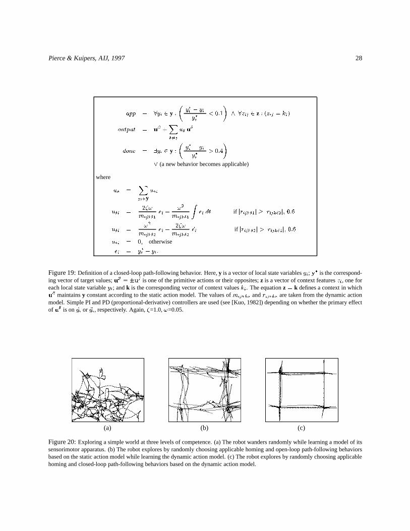
Pierce & Kuipers, AIJ, 1997 28
app � 8yi 2 y :
�jy�i � yij
y�i< 0:1
�^ 8zij 2 z : (zij = ki)
output = u� +XÆ 6=j
uÆ uÆ
done = 9yi 2 y :
�jy�i � yij
y�i> 0:4
�
_ (a new behavior becomes applicable)
where
uÆ =Xyi2y
uÆi
uÆi =2�!
mijkÆ1
ei +!2
mijkÆ1
Zei dt if jrijkÆ1j � jrijkÆ2j; 0:6
uÆi =!2
mijkÆ2
ei +2�!
mijkÆ2
_ei if jrijkÆ2j > jrijkÆ1j; 0:6
uÆi = 0; otherwise
ei = y�i � yi:
Figure 19:Definition of a closed-loop path-following behavior. Here,y is a vector of local state variablesyi; y� is the correspond-ing vector of target values;u� = �uj is one of the primitive actions or their opposites;z is a vector of context featureszi, one foreach local state variableyi; andk is the corresponding vector of context valueski. The equationz = k defines a context in whichu� maintainsy constant according to the static action model. The values ofmijkÆn andrijkÆn are taken from the dynamic action
model. Simple PI and PD (proportional-derivative) controllers are used (see [Kuo, 1982]) depending on whether the primary effectof uÆ is on _yi or �yi, respectively. Again,�=1.0,!=0.05.
(a) (b) (c)
Figure 20:Exploring a simple world at three levels of competence. (a) The robot wanders randomly while learning a model of itssensorimotor apparatus. (b) The robot explores by randomly choosing applicable homing and open-loop path-following behaviorsbased on the static action model while learning the dynamic action model. (c) The robot explores by randomly choosing applicablehoming and closed-loop path-following behaviors based on the dynamic action model.

Pierce & Kuipers, AIJ, 1997 29
The learning methods are first demonstrated for the mobile robot in a cluttered room. Then, to demonstrate thatthe learned model of the sensorimotor apparatus applies beyond the particular environment in which the model waslearned, the learning agent is transferred to a new, T-shaped environment after its control-level learning has beenerased. Here it re-learns the control level and demonstrate a set of learned path-following behaviors. Finally, todemonstrate that the learning of the control level applies beyond the particular environment in which it was learned,the learning agent is transferred to an empty room where it again demonstrates the learned path-following behaviors.
Sections 6.4 and 6.5 describe two experiments in which various of the learning methods failed and explain whythey failed. Section 6.4 describes an experiment in which the image-feature generator fails to produce a ring-shapedrepresentation of the structure of the ring of distance sensors. Section 6.5 describes an experiment in which the learningagent fails to discover any local state variables. Section 6.6 summarizes the ways in which the learning methods canfail. Finally, Section 6.7 identifies a number of ways in which the learning methods can be improved.
6.1 A cluttered room
The environment used in this experiment is a rectangular room with dimensions six meters by four meters, containingfour rectangular obstacles (Figure 23). The simulated mobile robot used throughout this section is the same as thatdescribed in Section 2.1.
6.1.1 Modeling the sensory apparatus
The first step in modeling the robot’s sensory apparatus is to apply the group-feature generator. The learning agentcomputes distance metricsd1 andd2 after wandering for 20 minutes. Their values are qualitatively similar to thoseshown in Figure 2. The group-feature generator identifies the same groups as those in Section 2.3. The second step inmodeling the robot’s sensory apparatus is to apply the image-feature generator. The learning agent computes distancemetricd1 for the group of 23 related sensors after wandering for 40 minutes.21 The outputs of the metric scaling andrelaxation algorithm are qualitatively similar to those shown in Figure 3.
6.1.2 Modeling the motor apparatus
The first step in modeling the robot’s motor apparatus is to characterize the effects of each of a large set of representa-tive motor control vectors. In this experiment, 100 representative motor control vectors of unit magnitude are chosen.Eight exampleamvf’s and their associated motor control vectors are shown in Figure 21. These were obtained whilethe learning agent wandered for 60 minutes, repeatedly choosing a representative motor control vector at random andexecuting it for one second (ten time steps). The first four eigenvectors produced by principal component analysisfrom are shown in Figure 22. The first corresponds to a pure rotation motion and the second corresponds to a puretranslation motion. The two motor control vectors identified as primitive actions are shown above under the two prin-cipal eigenvectors. None of the other eigenvectors match any of theamvf’s. Notice that the primitive actions identifiedhere very closely match those shown in Figure 7. The result of the analysis is that the robot’s motor apparatus has twodegrees of freedom and that the above primitive actions can be used to produce motion for each degree of freedom.
6.1.3 Learning behaviors
As described in Section 4, the learning agent identifies the set of local-minimum features (s-g-im-lmin-tr-val) as localstate variables (they are the only generated features that are identified as both action dependent and predictable).
The learned static and dynamic action models are qualitatively similar to those learned in Sections 4 and 5. In thisexperiment, the learning agent again discovers that it can use the first (turning) primitive action for error correctionwhile executing an open-loop path-following behavior based on the second (advancing) primitive action. It uses thisinformation to define closed-loop path-following behaviors. Figure 23 shows a trace of a random exploration behaviordemonstrating the learning agent’s learned behaviors.
21We use fairly long wandering periods so that the robot adequately explores its state space. For the uncluttered, rectangular room, shorter periodswere used because the group- and image-feature generators quickly converged. See Section 6.7 for a discussion of improved feature generators thatautomatically detect when they have converged.

Pierce & Kuipers, AIJ, 1997 30
(1.00 -0.00) (0.69 0.73) (0.00 1.00) (-0.73 0.69)
(-1.00 0.00) (-0.69 -0.73) (-0.00 -1.00) (0.73 -0.69)
Figure 21:Exampleamvf’s and associated motor control vectors for the cluttered-room experiment.
1.40 1.10 0.27 0.22
u0= (-0.706 0.707) u
1= (0.728 0.683)
Figure 22:The first four eigenvectors and the primitive actions for the cluttered-room experiment.
Figure 23:The path taken by the robot while the learning agent randomly selects learned homing and path-following behaviors.When no other behavior is applicable, it randomly selects primitive actions. The robot is initially in the middle. The learning agentbegins by using a homing behavior to move toward the long obstacle and then using a path-following behavior to move along it.The diagonal trajectories in the corners are the results of homing behaviors that move the robot from a wall to a path.
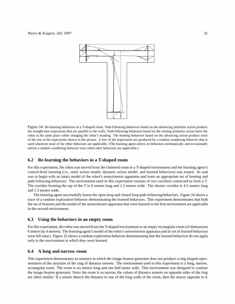
Pierce & Kuipers, AIJ, 1997 31
Figure 24:Re-learning behaviors in a T-shaped room. Path-following behaviors based on the advancing primitive action producethe straight-line trajectories that are parallel to the walls. Path-following behaviors based on the turning primitive action leave therobot in the same place while changing the robot’s heading. The homing behaviors based on the advancing action produce mostof the rest of the trajectories shown in the picture. A few of the trajectories are produced by a random wandering behavior that isused whenever none of the other behaviors are applicable. (The learning agent selects its behaviors stochastically and occasionallyselects a random wandering behavior even when other behaviors are applicable.)
6.2 Re-learning the behaviors in a T-shaped room
For this experiment, the robot was moved from the cluttered room to a T-shaped environment and the learning agent’scontrol-level learning (i.e., static action model, dynamic action model, and learned behaviors) was erased. Its taskwas to begin with an intact model of the robot’s sensorimotor apparatus and learn an appropriate set of homing andpath-following behaviors. The environment used in this experiment consists of two corridors connected to form a T.The corridor forming the top of the T is 6 meters long and 1.5 meters wide. The shorter corridor is 4.5 meters longand 1.5 meters wide.
The learning agent successfully learns the open-loop and closed-loop path-following behaviors. Figure 24 shows atrace of a random exploration behavior demonstrating the learned behaviors. This experiment demonstrates that boththe set of features and the model of the sensorimotor apparatus that were learned in the first environment are applicablein the second environment.
6.3 Using the behaviors in an empty room
For this experiment, the robot was moved from the T-shaped environment to an empty rectangular room (of dimensions6 meters by 4 meters). The learning agent’s model of the robot’s sensorimotor apparatus and its set of learned behaviorswere left intact. Figure 25 shows a random exploration behavior demonstrating that the learned behaviors do not applyonly to the environment in which they were learned.
6.4 A long and narrow room
This experiment demonstrates an instance in which the image-feature generator does not produce a ring-shaped repre-sentation of the structure of the ring of distance sensors. The environment used in this experiment is a long, narrow,rectangular room. The room is six meters long and one half meter wide. This environment was designed to confusethe image-feature generator. Since the room is so narrow, the values of distance sensors on opposite sides of the ringare often similar: If a sensor detects the distance to one of the long walls of the room, then the sensor opposite to it

Pierce & Kuipers, AIJ, 1997 32
Figure 25:Using the learned homing and path-following behaviors in an empty room.
00.20.40.60.81
1.21.41.61.82
1 2 3 4 5 6 7 8 9 10
Metric scaling eigenvalues
012
345
6
78910
1112
13
141516
1718
19
212223
01
23
45
6
7
8910
111213
1415
1617
18 19
212223
Figure 26:The outputs of the metric-scaling and relaxation algorithms for the narrow-room experiment.
detects the distance to the wall on the opposite side of the room. Both sensors produce a small value (less than 0.5).On the other hand, if a sensor returns a large value, then there is a good chance that the sensor opposite to it will alsoreturn a large value.
If opposite sensors return similar values, on average, then the image-feature generator will place them close to-gether in the image feature. It is unlikely, in this case, that the image feature will capture the ring structure of the arrayof distance sensors.
6.4.1 Modeling the sensory apparatus
The result of the group-feature generator is the same as before: The distance sensors are all grouped together. Theoutputs of the metric scaling and relaxation algorithm are shown in Figure 26. According to the metric-scaling screediagram on the left, the structure of the array of sensors is best captured by a four-dimensional representation – there isno arrangement of points in fewer than four dimensions for which the distance between any two points approximatesthe distance between corresponding sensors as measured by distance metricd1. The middle figure below shows theprojection onto two dimensions of the set of points generated by the metric-scaling algorithm. The figure on the rightshows the results of the relaxation algorithm.22 Notice that sensors that are adjacent in the ring of sensors are closetogether in the image.23
22The metric-scaling algorithm, the relaxation algorithm, and the definition of the image and motion features can all handle images of arbitrarydimension. However, in the current implementation, we have constrained the image feature to be two-dimensional. A goal for future research is toremove this artificial constraint and test the methods on sensory arrays that are genuinely three-dimensional.
23Though the results are not shown here, we have also run the relaxation algorithm for this distance metric in three dimensions. In that case theresulting pattern of sensors resembles the pattern of stitching on a baseball.
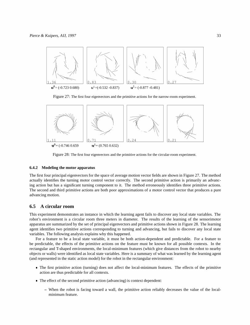
Pierce & Kuipers, AIJ, 1997 33
1.36 0.83 0.30 0.27
u0= (-0.723 0.680) u
1=(-0.532 -0.837) u2= (-0.877 -0.481)
Figure 27:The first four eigenvectors and the primitive actions for the narrow-room experiment.
1.11 0.71 0.24 0.21
u0= (-0.746 0.659 u
1= (0.765 0.632)
Figure 28:The first four eigenvectors and the primitive actions for the circular-room experiment.
6.4.2 Modeling the motor apparatus
The first four principal eigenvectors for the space of average motion vector fields are shown in Figure 27. The methodactually identifies the turning motor control vector correctly. The second primitive action is primarily an advanc-ing action but has a significant turning component to it. The method erroneously identifies three primitive actions.The second and third primitive actions are both poor approximations of a motor control vector that produces a pureadvancing motion.
6.5 A circular room
This experiment demonstrates an instance in which the learning agent fails to discover any local state variables. Therobot’s environment is a circular room three meters in diameter. The results of the learning of the sensorimotorapparatus are summarized by the set of principal eigenvectors and primitive actions shown in Figure 28. The learningagent identifies two primitive actions corresponding to turning and advancing, but fails to discover any local statevariables. The following analysis explains why this happened.
For a feature to be a local state variable, it must be both action-dependent and predictable. For a feature tobe predictable, the effects of the primitive actions on the feature must be known for all possible contexts. In therectangular and T-shaped environments, the local-minimum features (which give distances from the robot to nearbyobjects or walls) were identified as local state variables. Here is a summary of what was learned by the learning agent(and represented in the static action model) for the robot in the rectangular environment:
� The first primitive action (turning) does not affect the local-minimum features. The effects of the primitiveaction are thus predictable for all contexts.
� The effect of the second primitive action (advancing) is context dependent:
– When the robot is facing toward a wall, the primitive action reliably decreases the value of the local-minimum feature.
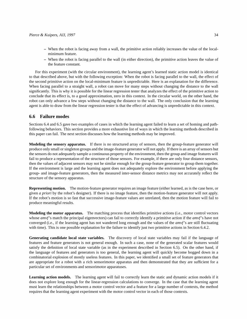
Pierce & Kuipers, AIJ, 1997 34
– When the robot is facing away from a wall, the primitive action reliably increases the value of the local-minimum feature.
– When the robot is facing parallel to the wall (in either direction), the primitive action leaves the value ofthe feature constant.
For this experiment (with the circular environment), the learning agent’s learned static action model is identicalto that described above, but with the following exception: When the robot is facing parallel to the wall, the effect ofthe second primitive action on the local-minimum feature is unpredictable. Here is an explanation for the difference.When facing parallel to a straight wall, a robot can move for many steps without changing the distance to the wallsignificantly. This is why it is possible for the linear regression tester that analyzes the effect of the primitive action toconclude that its effect is, to a good approximation, zero in this context. In the circular world, on the other hand, therobot can only advance a few steps without changing the distance to the wall. The only conclusion that the learningagent is able to draw from the linear regression tester is that the effect of advancing is unpredictable in this context.
6.6 Failure modes
Sections 6.4 and 6.5 gave two examples of cases in which the learning agent failed to learn a set of homing and path-following behaviors. This section provides a more exhaustive list of ways in which the learning methods described inthis paper can fail. The next section discusses how the learning methods may be improved.
Modeling the sensory apparatus. If there is no structured array of sensors, then the group-feature generator willproduce only small or singleton groups and the image-feature generator will not apply. If there is an array of sensors butthe sensors do not adequately sample a continuous property of the environment, then the group and image features willfail to produce a representation of the structure of those sensors. For example, if there are only four distance sensors,then the values of adjacent sensors may not be similar enough for the group-feature generator to group them together.If the environment is large and the learning agent does not adequately explore the environment before applying thegroup- and image-feature generators, then the measured inter-sensor distance metrics may not accurately reflect thestructure of the sensory apparatus.
Representing motion. The motion-feature generator requires an image feature (either learned, as is the case here, orgivena priori by the robot’s designer). If there is no image feature, then the motion-feature generator will not apply.If the robot’s motion is so fast that successive image-feature values are unrelated, then the motion feature will fail toproduce meaningful results.
Modeling the motor apparatus. The matching process that identifies primitive actions (i.e., motor control vectorswhoseamvf’s match the principal eigenvectors) can fail to correctly identify a primitive action if theamvf’s have notconverged (i.e., if the learning agent has not wandered long enough and the values of theamvf’s are still fluctuatingwith time). This is one possible explanation for the failure to identify just two primitive actions in Section 6.4.2.
Generating candidate local state variables. The discovery of local state variables may fail if the language offeatures and feature generators is not general enough. In such a case, none of the generated scalar features wouldsatisfy the definition of local state variable (as in the experiment described in Section 6.5). On the other hand, ifthe language of features and generators is too general, the learning agent will quickly become bogged down in acombinatorial explosion of mostly useless features. In this paper, we identified a small set of feature generators thatare appropriate for a robot with a rich sensorimotor apparatus and then demonstrated that they are sufficient for aparticular set of environments and sensorimotor apparatuses.
Learning action models. The learning agent will fail to correctly learn the static and dynamic action models if itdoes not explore long enough for the linear-regression calculations to converge. In the case that the learning agentmust learn the relationships between a motor control vector and a feature for a large number of contexts, the methodrequires that the learning agent experiment with the motor control vector in each of those contexts.

Pierce & Kuipers, AIJ, 1997 35
Learning path-following behaviors. The learning of path-following behaviors can depend on the set of learnedprimitive actions. If none of the primitive actions can be used to maintain any of the local state variables constant, thenno path-following behaviors will be learned.
In the experiments described in this paper, each learning method builds on the results of the preceding methods,which means that one source of failure for a method is the failure of a preceding method. This observation, if leftunqualified, sells the learning methods short. First, the methods are interesting in their own right (for example, themodeling of the motor apparatus could be applied to a sensory system whose structure was given by the robot’sdesigner rather than being learned). Second, the sequential nature of the learning is partially an artifact of our particularlearning problem. For example, the discovery of local state variables does not, in general, depend on the success ofthe image-feature generator but is instead the result of an independent process of generate and test.
6.7 Future work
Section 6.6 identified a number of ways in which the learning methods can fail. This section provides suggestions forimprovements to the learning methods.
Improved feature testers. One way that several of the learning methods can fail is by jumping to a conclusion pre-maturely. For example, if the group-feature generator uses a distance metric before the distance metric has converged,then the output of the generator may be incorrect. If primitive actions are identified before theamvf’s have converged,then the model of the motor apparatus may be incorrect.
In these examples, the distance metrics and theamvf’s are examples offeature testers— features that are used tocharacterize other features. A solution to the problem of drawing premature conclusions is to have each feature testertell when its output is meaningful. It can do this by providing a measure of confidence in addition to its output value.For example, the confidence level for a tester might be close to 1 if the tester’s output is stable (changing slowly) andclose to 0 if the tester’s output is still fluctuating.
For a linear regression tester, the confidence level should be a function of the set of inputs it has received. Consider,for example, how the static action model uses linear regression testers. It uses a separate linear regression tester foreachhfeature, primitive action, contexti triple. If the robot is never in a given context, then the confidence level for anylinear regression tester based on that context should be zero. The confidence level for a linear regression tester mightbe defined in terms of the90% confidence interval24 for the correlation between the input variables. The smaller theconfidence interval, the greater the tester’s confidence level. Associating confidence levels with features could improveall of the learning steps listed in the previous section by reducing the chance of producing inaccurate or incompletemodels.
An improved static action model. The learning agent uses the static action model to define a set of open-loop path-following behaviors — behaviors that move the robot while maintaining a local state variable constant. In the currentimplementation, open-loop path-following behaviors are based on primitive actions. If a primitive action maintains alocal state variable constant, according to the static action model, then it can be used as the “base action” for a path-following behavior. Using only primitive actions as base actions is a limitation of the current implementation. Themethod for learning path-following behaviors would be improved if the static action model could predict the effects ofarbitrary motor control vectors, not just the primitive actions. With a more comprehensive static action model, morepath-following behaviors could be defined. For example, in the circular room, a path-following behavior could bebased on a motor control vector with a large advancing component and a small turning component.
One approach to improving the static action model would be to discretize the space of all motor control vectorsinto a set of representative motor control vectors and then to learn models of all of these instead of just the primitiveactions. Another approach would be to use a neural network [Jordan and Rumelhart, 1992] to learn to predict thecontext-dependent effects of arbitrary actions. The network could then serve as the static action model and could beused to find base actions for path-following behaviors.
24See, for example, [Krzanowski, 1988, p. 415].
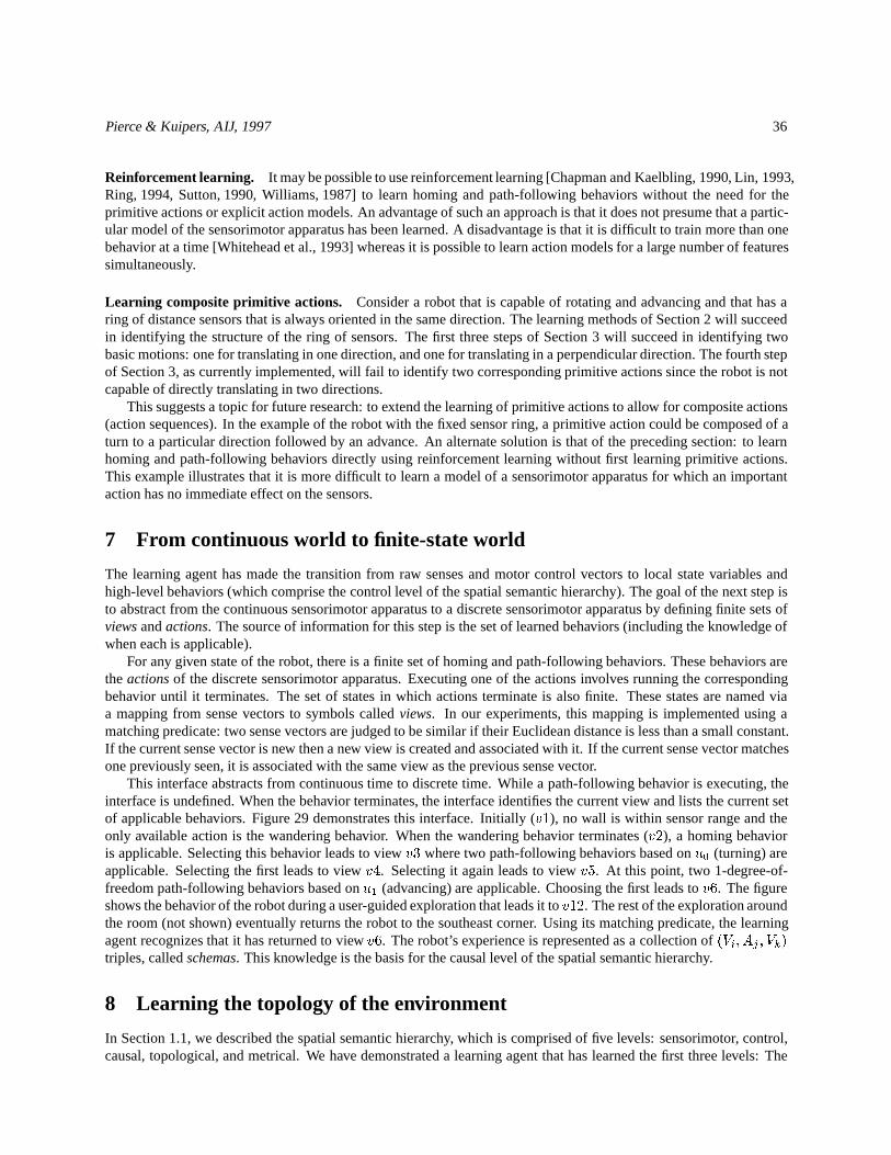
Pierce & Kuipers, AIJ, 1997 36
Reinforcement learning. It may be possible to use reinforcement learning [Chapman and Kaelbling, 1990, Lin, 1993,Ring, 1994, Sutton, 1990, Williams, 1987] to learn homing and path-following behaviors without the need for theprimitive actions or explicit action models. An advantage of such an approach is that it does not presume that a partic-ular model of the sensorimotor apparatus has been learned. A disadvantage is that it is difficult to train more than onebehavior at a time [Whitehead et al., 1993] whereas it is possible to learn action models for a large number of featuressimultaneously.
Learning composite primitive actions. Consider a robot that is capable of rotating and advancing and that has aring of distance sensors that is always oriented in the same direction. The learning methods of Section 2 will succeedin identifying the structure of the ring of sensors. The first three steps of Section 3 will succeed in identifying twobasic motions: one for translating in one direction, and one for translating in a perpendicular direction. The fourth stepof Section 3, as currently implemented, will fail to identify two corresponding primitive actions since the robot is notcapable of directly translating in two directions.
This suggests a topic for future research: to extend the learning of primitive actions to allow for composite actions(action sequences). In the example of the robot with the fixed sensor ring, a primitive action could be composed of aturn to a particular direction followed by an advance. An alternate solution is that of the preceding section: to learnhoming and path-following behaviors directly using reinforcement learning without first learning primitive actions.This example illustrates that it is more difficult to learn a model of a sensorimotor apparatus for which an importantaction has no immediate effect on the sensors.
7 From continuous world to finite-state world
The learning agent has made the transition from raw senses and motor control vectors to local state variables andhigh-level behaviors (which comprise the control level of the spatial semantic hierarchy). The goal of the next step isto abstract from the continuous sensorimotor apparatus to a discrete sensorimotor apparatus by defining finite sets ofviewsandactions. The source of information for this step is the set of learned behaviors (including the knowledge ofwhen each is applicable).
For any given state of the robot, there is a finite set of homing and path-following behaviors. These behaviors aretheactionsof the discrete sensorimotor apparatus. Executing one of the actions involves running the correspondingbehavior until it terminates. The set of states in which actions terminate is also finite. These states are named viaa mapping from sense vectors to symbols calledviews. In our experiments, this mapping is implemented using amatching predicate: two sense vectors are judged to be similar if their Euclidean distance is less than a small constant.If the current sense vector is new then a new view is created and associated with it. If the current sense vector matchesone previously seen, it is associated with the same view as the previous sense vector.
This interface abstracts from continuous time to discrete time. While a path-following behavior is executing, theinterface is undefined. When the behavior terminates, the interface identifies the current view and lists the current setof applicable behaviors. Figure 29 demonstrates this interface. Initially (v1), no wall is within sensor range and theonly available action is the wandering behavior. When the wandering behavior terminates (v2), a homing behavioris applicable. Selecting this behavior leads to viewv3 where two path-following behaviors based onu0 (turning) areapplicable. Selecting the first leads to viewv4. Selecting it again leads to viewv5. At this point, two 1-degree-of-freedom path-following behaviors based onu1 (advancing) are applicable. Choosing the first leads tov6. The figureshows the behavior of the robot during a user-guided exploration that leads it tov12. The rest of the exploration aroundthe room (not shown) eventually returns the robot to the southeast corner. Using its matching predicate, the learningagent recognizes that it has returned to viewv6. The robot’s experience is represented as a collection of(Vi; Aj ; Vk)triples, calledschemas. This knowledge is the basis for the causal level of the spatial semantic hierarchy.
8 Learning the topology of the environment
In Section 1.1, we described the spatial semantic hierarchy, which is comprised of five levels: sensorimotor, control,causal, topological, and metrical. We have demonstrated a learning agent that has learned the first three levels: The
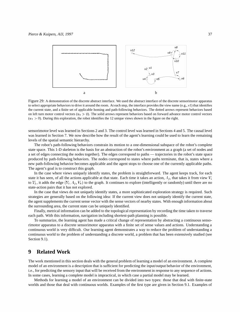
Pierce & Kuipers, AIJ, 1997 37
v1v2
v3
v4 v5 v6
v7
v8
v9
v10
v11v12
a b
Figure 29:A demonstration of the discrete abstract interface. We used the abstract interface of the discrete sensorimotor apparatusto select appropriate behaviors to drive it around the room. At each step, the interface provides the view name (e.g.,v1) that identifiesthe current state, and a finite set of applicable homing and path-following behaviors. The dotted arrows represent behaviors basedon left turn motor control vectors (u0 > 0). The solid arrows represent behaviors based on forward advance motor control vectors(u1 > 0). During this exploration, the robot identifies the 12 unique views shown in the figure on the right.
sensorimotor level was learned in Sections 2 and 3. The control level was learned in Sections 4 and 5. The causal levelwas learned in Section 7. We now describe how the result of the agent’s learning could be used to learn the remaininglevels of the spatial semantic hierarchy.
The robot’s path-following behaviors constrain its motion to a one-dimensional subspace of the robot’s completestate space. This 1-D skeleton is the basis for an abstraction of the robot’s environment as a graph (a set of nodes anda set of edges connecting the nodes together). The edges correspond to paths — trajectories in the robot’s state spaceproduced by path-following behaviors. The nodes correspond to states where paths terminate, that is, states where anew path-following behavior becomes applicable and the agent stops to choose one of the currently applicable paths.The agent’s goal is to construct this graph.
In the case where views uniquely identify states, the problem is straightforward. The agent keeps track, for eachstate it has seen, of all the actions applicable at that state. Each time it takes an action,Aj , that takes it from viewVito Vk , it adds the edge(Vi; Aj ; Vk) to the graph. It continues to explore (intelligently or randomly) until there are nostate-action pairs that it has not explored.
In the case that views do not uniquely identify states, a more sophisticated exploration strategy is required. Suchstrategies are generally based on the following idea: If the current view does not uniquely identify the current state,the agent supplements the current sense vector with the sense vectors of nearby states. With enough information aboutthe surrounding area, the current state can be uniquely identified.
Finally, metrical information can be added to the topological representation by recording the time taken to traverseeach path. With this information, navigation including shortest-path planning is possible.
To summarize, the learning agent has made a critical change of representation by abstracting a continuous senso-rimotor apparatus to a discrete sensorimotor apparatus with a finite set of sense values and actions. Understanding acontinuous world is very difficult. Our learning agent demonstrates a way to reduce the problem of understanding acontinuous world to the problem of understanding a discrete world, a problem that has been extensively studied (seeSection 9.1).
9 Related Work
The work mentioned in this section deals with the general problem of learning a model of an environment. A completemodel of an environment is a description that is sufficient for predicting the input/output behavior of the environment,i.e., for predicting the sensory input that will be received from the environment in response to any sequence of actions.In some cases, learning a complete model is impractical, in which case a partial model may be learned.
Methods for learning a model of an environment can be divided into two types: those that deal with finite-stateworlds and those that deal with continuous worlds. Examples of the first type are given in Section 9.1. Examples of

Pierce & Kuipers, AIJ, 1997 38
the second type are given in Section 9.2. Our contribution has been to show how a learning agent can abstract a robot’scontinuous world to a finite-state world to which finite-state learning methods may be applied.
9.1 Inferring the structure of finite-state worlds
The task of inferring the structure of a finite-state environment is the task of finding a finite-state automaton that ac-curately captures the input-output behavior of the environment. In the case that the learning agent is passively givenexamples of the environment’s input/output behavior, it has been shown that finding the smallest automaton consis-tent with the behavior is NP-complete [Angluin, 1978, Gold, 1978]. With active learning, in which the agent activelychooses its actions, the problem becomes tractable. Kuipers [Kuipers, 1978] describes the TOUR model, a method forunderstanding discrete spatial worlds based on a theory of cognitive maps. Dudek, et al. [Dudek et al., 1991] general-ize Kuipers and Byun’s [Kuipers and Byun, 1988, Kuipers and Byun, 1991] strategy for topological map-learning andprovide algorithms for discriminating perceptually identical states. Angluin [Angluin, 1987] gives a polynomial-timealgorithm using active experimentation and passively received counterexamples. Rivest & Schapire [Rivest and Schapire, 1993]improve on Angluin’s algorithm and give a version that does not require the reset operation (returning to the start stateafter each experiment).
Dean et al. [Dean et al., 1992] have extended Rivest and Schapire’s theory to handle stochastic FSA’s. They as-sume that actions are deterministic but that the output function mapping states to senses is probabilistic. The key totheir method is “going in circles” until the uncertainty washes out. Dean, Basye, and Kaelbling [Dean et al., 1993]give a good review of learning techniques for a variety of stochastic automata. Drescher’s schema mechanism[Drescher, 1991] employs a statistical learning method called marginal attribution. Schemas emphasize sensory effectsof actions rather than state transitions and are ideal for representing partial knowledge in stochastic worlds.
Wei-Min Shen’s LIVE system [Shen, 1994] learns the structure of a finite-state environment from experience (andexperimentation) within it. His complementary discrimination learning algorithm exploits observed counterexamplesto a hypothesized concept definition to refine the boundary between positive and negative examples of the concept.When the environment is only partially observable, LIVE uses locally distinguishing experiments to test the hypothe-sized properties of unobserved state variables.
A primary focus of the work of Shen and other constructive inductionists [Hiraki, 1994, Matheus, 1991, Shen, 1990,Shen and Simon, 1989] is the learning of new features. At this level of description, our approach and Shen’s are sim-ilar. However, in terms of the actual methods used and the domains of applicability, the two approaches are verydifferent and are in fact complementary.
We focus on feature-learning methods applicable to robots with continuous-valued sensors and control signalssituated in a 2-dimensional approximation of a 3-dimensional world. We provide a language of features and generatorsespecially suitable for robots with structured arrays of sensors. Our emphasis is on learning of sensory features andcontinuous control laws. Shen, on the other hand, focuses on learning rules (consisting of conditions, actions, andpredictions) that are expressed symbolically. The conditions and predictions are expressed in terms of “percepts,”which are high-level, symbolic descriptions (e.g., ON(disk, peg)). The actions may have continuous parameters (e.g.,rotate(�)), but each action is atomic rather than continuous.
The two approaches might be combined in the following way: a learning agent first uses our methods to learn tonavigate using its continuous sensorimotor apparatus, viewing the world in terms of discrete states and actions. It thenuses Shen’s methods to learn relationships expressed in terms of these states and actions and to acquire nonspatialknowledge such as the effects of pushing objects, flipping switches, or opening doors.
A more specific example of a potential combination of the two approaches is the use of Shen’s complementarydiscrimination learning in learning context-dependent action models (see Section 4.2.3). We currently use a brute-force method for determining whether a control signalu has a predictable effect on a given featurex. The methodinvolves testing a large set of features to see if any can be used to define a partition of the robot’s state space as a setof contexts such that in each context there is a simple, linear relationship betweenu andx. We expect that methodssuch as Shen’s complementary discrimination learning could be used to generate such partitions more efficiently andmore intelligently.

Pierce & Kuipers, AIJ, 1997 39
9.2 Inferring the structure of continuous worlds
Applying finite-state automaton learning methods to the real world or a continuous simulation of it requires an ab-straction from a continuous environment to a discrete representation. Kuipers and Byun [Kuipers and Byun, 1988,Kuipers and Byun, 1991] demonstrate an engineered solution to the continuous-to-discrete abstraction problem forthe NX robot. NX’sdistinctive placescorrespond to discrete states and itslocal control strategiescorrespond to statetransitions. These constructs have to be manually redesigned in order to apply to a robot with a different sensorimotorapparatus. Mataric [Mataric, 1991, Mataric, 1992] and Kortenkamp & Weymouth [Kortenkamp and Weymouth, 1994]have engineered similar solutions on physical robots.
Lin and Hanson [Lin and Hanson, 1993] use a physical robot, called Ratbot, with 16 sonar sensors and 16 infraredsensors to demonstrate learning of a topological map of locally distinctive places. Their work is inspired by the workof Kuipers and Byun, but they use reinforcement learning25 to train the local control strategies, rather than engineeringthem by hand. The target behaviors (e.g., corridor following) are specified by a human teacher. For example, whenlearning the corridor-following behavior, the robot is rewarded when it moves along the corridor without running intoobstacles.
Our approach [Pierce, 1991a, Pierce, 1991b, Pierce, 1995, Pierce and Kuipers, 1994] is complementary to that ofLin and Hanson. They specify the desirable behaviors by defining appropriate reward signals and then letting the robotlearn on its own how to gain the rewards. Our learning agent, on the other hand, specifies its own target behaviors,eliminating the need for the human teacher. It does this by first learning a set of local state variables and then using themto define a set of error signals. Homing and path-following behaviors are then specified as behaviors that minimize theerror signals or move the robot while maintaining them near zero. All of this is accomplished in a domain-independentmanner — the robot does not need to be given any knowledge about corridors or corridor-following behaviors.
Once the error signals are defined, there are a number of ways in which the homing and path-following behaviorsmight be learned. Reinforcement learning is one approach.26 The approach used in this paper is to learn static anddynamic action models that characterize the effects of actions on the local state variables and then to use these modelsto directly define the homing and path-following behaviors. This approach does require that the learning agent be givensome knowledge of control theory, but the required knowledge consists of domain-independent templates. It would beinteresting to combine our approach with that used by Lin & Hanson’s Ratbot to produce a learning method that usesneither domain-dependent knowledge nor a knowledge of control theory. The error signals would be defined as for ourlearning agent and a neural-net version of Q learning would be used to learn the local control strategies based on thoseerror signals. The control laws would be implemented as mappings from sensory inputs to motor control signals. Ifthe sensory inputs include the error signals, their derivatives, and their integrals, then the set of control laws that canbe defined in this way includes the PI and PD control laws used by our implemented learning agent.
An important difference between our approach and that of Lin and Hanson is that our approach handles contextdependence at the feature level rather than at the behavior level: Our learning agent learns, given the current context,the effects of each primitive action on each feature. Lin and Hanson’s learning agent learns, given the current context,which action to take in order to produce a particular behavior. There are two advantages to learning at the feature level.First, what is learned about one feature may be used to define multiple behaviors, e.g., a homing behavior (in whicha primitive action is used to increase or decrease the value of the feature) and a path-following behavior (in whicha primitive action is used to move while maintaining the feature constant). Second, the learning agent can learn theeffects of motor control signals on multiple features simultaneously, whereas it is only possible for Lin and Hanson’slearning agent to learn one behavior at a time.
10 Discussion
10.1 What is the value of an existence proof?
As discussed in Section 1.3, the results presented here are an existence proof, demonstrating one path from the begin-ning to the end of a complex learning problem. Once a single path has been demonstrated, however narrow, future
25The reinforcement-learning algorithm is a neural-network version of Q learning [Watkins, 1989, Lin, 1993].26In earlier work we explored the use of reinforcement learning to learn homing behaviors [Pierce and Kuipers, 1991].
Pierce & Kuipers, AIJ, 1997 40
research can broaden the way and find alternate routes.We have made some progress toward assessing the width and solidity of the path, first by applying the same
learning methods to a significantly different robot (Section 2.5), and second by applying our methods to a variety ofdifferent environments systematically designed to demonstrate both success and failure of the methods (Section 6).This is a step toward determining how much and what type of sensory input a robot must have to learn a meaningfulcognitive map of a continuous environment, and how observable and predictable the environment must be for the robotto be able to comprehend it.
The existence proof demonstrates that a hard and interesting learning problem may have a heterogeneous solution,combining the strengths of several focused learning algorithms. While this solution does rely on a number of assump-tions about the sensorimotor system and the environment (Section 6.6), we believe that several of those assumptionscan be eliminated by future research (Section 6.7). An irreducible minimum set of assumptions would be a significantscientific result.
10.2 Why learn what can be programmed directly?
This paper has shown, among other things, how a learning agent can learn a model of its sensorimotor apparatus.There are several reasons why it is worthwhile to take the trouble to learn what could be directly programmed by arobot’s designer.
Sensor variation and failure. Direct programming does not take sensor failure into consideration. For example, ifone of a set of distance sensors fails, the learning methods will accommodate the failure with no additional humanintervention. These methods will also accommodate random variation in the position or direction of distance sensors.Such variation is inevitable if robots are mass produced.
Generality. Ideally, one learning algorithm applies to many different types of sensorimotor apparatuses and thus canreplace the process of designing a particular solution for each sensorimotor apparatus.
A deeper understanding of the problem domain. The design of the learning agent required the identification ofsources of information that could be exploited by the learning agent and the development of general-purpose learn-ing algorithms to exploit that information. These sources of information and learning algorithms comprise a deeperunderstanding of the problem domain.27
10.3 What about innate goals?
We have characterized a robot in terms of its set of sensors and effectors, without concern for its innate goals (e.g.,survival, curiosity, pain avoidance). The learning methods we have developed function by observing the sensory effectsof actions, either during a random walk through the environment (as described in this paper) or during goal-directedbehavior.
Reactive behavior in pursuit of innate goals can support the learning methods described here. With a goal such aspain avoidance, for example, a learning agent might quickly learn a reflexive behavior for obstacle avoidance. Sucha behavior would help keep the learning agent out of danger as it applies the higher-level learning methods. On theother hand, by operating in the background of goal-directed behavior, the learning agent could receive a biased set ofexperiences and observations of the environment.
Conversely, the learned methods can serve as a foundation for goal-directed learning. When the agent has learnedhigher-level sensorimotor primitives, it can search for behaviors in an action space of larger granularity, describingthe environment at a higher level (see Figure 20), and making it easier to achieve innate goals such as survival andcuriosity.
27Of course, designing a learning agent does notguaranteea deeper understanding of the problem domain. An opaque method such as neuralnet or genetic algorithm learning could conceivably learn a model of its sensorimotor apparatus without teaching us anything about perception,behavior, or map building.
Pierce & Kuipers, AIJ, 1997 41
10.4 How general are the learning methods?
This paper has identified and demonstrated a number of generic methods for modeling and using an uninterpretedsensorimotor apparatus. This section lists several examples where a generic object or method is used that subsumes amore specific object or method but is more general because it makes fewer assumptions.
The learned features are based on a set of generic mathematical constructs (e.g., scalars, vectors, matrices, scalarfields, and vector fields) rather than on a human-generated list of salient properties of a robot’s environment. Themethod for identifying the structure of a sensory apparatus uses generic distance metrics that make no assumptionsabout what the sensors are sensing (for example, the method does not assume that the sensors measure distancesto objects). The method for characterizing the effects of motor control vectors is based on spatial and temporalderivatives, not motion of objects (which would require the identification and tracking of objects). The local statevariables learned by the learning agent in the example are defined in terms of the purely generic concept of localminimum, rather than the concept of distance-to-wall, which is only meaningful to the robot’s designer. The learnedcontrol laws are based on error signals derived from the learned local state variables – the learning agent of the exampleneeded no concept of wall when defining its path-following behaviors. The path-following behaviors are implementedusing generic control laws. The parameters used in the control laws are found by analyzing relationships betweencontrol signals and local state variables without any understanding of the meanings of the control signals or localstate variables. The views of the learning agent’s discrete abstract interface are the terminal states of path-followingbehaviors, as opposed to places meaningful only to the robot’s designer.
Related to the concept of generality is the concept of extensibility. The current implementation may be extendedby adding new types of features and feature generators. For example, new distance metrics could be used with thegroup-feature generator to capture new ways of distinguishing different types of sensors; the method for generatingand recognizing local state variables could be made more general by adding new feature generators.
10.5 Changes of representation
Each abstract interface that the agent learns provides a new representation to reason with.
� At the sensorimotor level, the group and image-feature generators analyze inter-sensor correlations to producethe image feature, which has substantially more structure than the raw sense vector.
The learned set of primitive actions provide a new representation of the robot’s motor capabilities that isgrounded in sensory effects.
� At the control level, behaviors and features are learned that are no longer purely egocentric. Whereas theprimitive actions are grounded in sensory effects averaged over time, the homing and path-following behaviorsare grounded in the structure of the external environment as reflected by the local state variables.
� At the causal level, the continuous state space is reduced to a finite set of states and trajectories, which can thenbe represented as the nodes and edges of a graph in the topological map.
11 Summary
This paper has presented a sequence of learning methods sufficient for learning a cognitive map of a robot’s continuousworld in the absence of domain-dependent knowledge of the robot’s sensorimotor apparatus or of the structure of itsworld. The reader may object that the sequence is tenuous: if any method failed, then the subsequent methods wouldnot even apply. While this is true, we maintain that each of the learning methods is interesting in its own rightand is applicable beyond the particular learning problem investigated here. Each learning method identifies a sourceof information available through experimentation with an uninterpreted sensorimotor apparatus and each provides amethod for exploiting that information to give the learning agent a new way of understanding the robot’s sensory inputor a new way of interacting with the robot’s environment.
The learning methods are summarized below and in Figure 30. Section 2 showed how to use the group and image-feature generators to learn a structural model of a sensory apparatus. They exploit the fact that, in a well engineered

Pierce & Kuipers, AIJ, 1997 42
Sensorimotor Level
Control Level
Causal Level
a0
a1
Raw senses and actions Sensory Structure
+
−
+
−u1 u0
Motion detection Primitive actions
< Vi, Aj, Vk >
Discrete Abstract Interface
Homing behaviors
y=y*
Open−looppath−followingbehaviors
Closed−looppath−followingbehaviors
StaticActionModel
LocalStateVariables Dynamic
ActionModel
Figure 30:A graphical summary of the learning methods used in this paper, showing the objects learned at each of the first threelevels of the spatial semantic hierarchy.

Pierce & Kuipers, AIJ, 1997 43
array of sensors sampling an almost-everywhere continuous property of the environment, the layout of the sensorsmay be reconstructed based on inter-sensor similarities. Section 3 showed how to use this structural knowledge tofirst define motion detectors and then use them to characterize the capabilities of a motor apparatus using a set ofprimitive actions, one for each of the robot’s degrees of freedom. Section 4 showed how to recognize local statevariables — scalar features whose derivatives can be approximated by context-dependent linear functions of the motorcontrol signals. The effects of the primitive actions on the local state variables are captured by the static actionmodel. Section 5 showed how to use the static action model to define homing and open-loop path-following behaviors,how to learn a dynamic action model to predict the effects of the primitive actions on the local state variables whileopen-loop path-following behaviors execute, and how to use the dynamic action model to define robust, closed-looppath-following behaviors. Finally, Section 7 showed how to use the homing and path-following behaviors to definea discrete abstract interface that allows the learning agent to abstract its continuous world to a finite-state world. Byusing the finite-state automaton as the target abstraction, the learning agent inherits a powerful set of methods forinferring the structure of its world.
In the biological world, the newly hatched organism embodies a great deal more knowledge than our learningagent. However, we hope that an exploration like that reported here will shed light on the structure and learnability offundamental knowledge about an agent’s relationship with its world. If so, it could provide insights into the evolution,development, and learning of spatial knowledge in biological organisms.
The potential for application of these methods to mechanical robots is much more direct. New robots, with newsensors and effectors, are being designed and built all the time. Robots will one day be sent into environmentsthat humans have never directly experienced (e.g., the deep ocean floor or the surface of another planet). For anewly-created robot to be able to orient itself to its sensorimotor system and its environment through autonomousexperimentation would be of substantial value. We believe that the methods presented here are a step in that direction.
A Computational Complexity
This appendix summarizes the complexities of the various learning methods described in this paper. The overallcomplexity of the sequence of learning methods is potentially exponential in the size of the raw sense vector and thedepth of the tree of generated features. In our experience, this level of complexity can be drastically reduced by usingan appropriate set of feature generators as is explained in Section A.3.
A.1 Modeling the sensory apparatus
Computing the distance metricd1 (used by both the group-feature generator and the image-feature generator) is ofcomplexityO(n2T ) wheren is the number of elements in the raw sense vector andT is the number of time stepstaken before the group-feature generator is applied. Computing the distance metricd2 (used by the group-featuregenerator) requires anO(1) computation for each element of the raw sense vector at each time step (to update thefrequency distributions) and anO(n2) computation when the group-feature generator is applied for a total complexityof O(nT + n2).
Identifying similar subgroups is anO(n2) computation. Using transitive closure to identify closed subgroups is anO(n3) computation. The metric-scaling is performed with an iterative algorithm for which each iteration involves anO(n3) computation. The relaxation algorithm is also iterative with each iteration beingO(n2). Since the dependenceof the number of iterations onn is unknown, these are lower limits on the actual complexities. In our experiments,Tis much greater thann so the overall complexity of the sensory-modeling step can be approximated byO(n2T ).28
A.2 Modeling the motor apparatus
The calculation of the motion feature requires anO(n2) computation at each time step. The calculation of theamvf’sis thus of complexityO(n2T ). The principal component analysis algorithm is of complexityO(n3). Again, sinceTis much greater thann, the overall complexity can be approximated byO(n2T ).
28An open problem is to predict the value of T for each learning method that requires an exploration phase.
Pierce & Kuipers, AIJ, 1997 44
A.3 Identifying local state variables
The first step in identifying local state variables is to generate new features. If every subset of the current set ofdefined features can be used to produce a new set of features, then the complexity of generating and testing featureswill be at leastO(2n) wheren is the number of elements of the raw sense vector. In our experience, this potentialcombinatorial explosion can be avoided by using an appropriate set of feature generators (e.g., generators that collapsemany input features into a small set of output features, or that only apply to certain types of features). For example,the group generator does not create arbitrary subsets of the raw sense vector – it creates at mostn non-overlappinggroup features.
The second step in identifying local state variables is to compute the static action model. The complexity of thecomputation of the action-dependent model isO(sT ) wheres is the number of singleton features that have beenlearned andT is the number of time steps over which the model is learned. The complexity of the computation of theaction-independent model isO(sTa) wherea is the number of primitive actions, The complexity of the computationof the context-dependent model isO(sTac) wherec is the average number of contexts associated with each feature.
A.4 Learning control laws
The number of open-loop path-following behaviors isO(vac) wherev is the number of learned local state variables,a is the number of primitive actions, andc is the average number of contexts associated with each local state variable.The complexity of the computation of the dynamic action model isO(vacT (a�1)). The number of generated closed-loop path-following behaviors (worst-case) isO(2va2c). In practice, the number of path-following behaviors can bemade much less than this upper bound. For example, the terms2v and2c can be replaced byv3 andc3 by only definingpath-following behaviors whose error vectors are based on at most three local state variables.
In our experiments, the number of path-following behaviors is kept reasonable by the following facts: (1) thenumber of learned local state variables is small and (2) the number of contexts in which a primitive action maintainsa local state variable constant is small relative to the total number of contexts. In our example,v is at most 3 andc isaround 20.
B Acknowledgments
The authors would like to thank Rick Froom, Wan Yik Lee, Risto Miikkulainen, Ray Mooney, Lyn Pierce, Mark Ring,Boaz Super, and two anonymous reviewers for their technical, editorial, and moral support.
References
[Angluin, 1978] Angluin, D. (1978). On the complexity of minimum inference of regular sets.Information andControl, 39:337–350.
[Angluin, 1987] Angluin, D. (1987). Learning regular sets from queries and counterexamples.Information andComputation, 75:87–106.
[Chapman and Kaelbling, 1990] Chapman, D. and Kaelbling, L. P. (1990). Learning from delayed reinforcement in acomplex domain. Tech. Report TR-90-11, Teleos Research, Palo Alto, California.
[Cormen et al., 1990] Cormen, T. H., Leiserson, C. E., and Rivest, R. L. (1990).Introduction to Algorithms. MITPress/McGraw-Hill Book Company, Cambridge, MA.
[Dean et al., 1992] Dean, T., Angluin, D., Basye, K., Engelson, S., Kaelbling, L., Kokkevis, E., and Maron, O. (1992).Inferring finite automata with stochastic output functions and an application to map learning. InProceedings, TenthNational Conference on Artificial Intelligence, pages 208–214, San Jose, CA. AAAI Press/MIT Press.

Pierce & Kuipers, AIJ, 1997 45
[Dean et al., 1993] Dean, T., Basye, K., and Kaelbling, L. (1993). Uncertainty in graph-based map learning. InConnell, J. H. and Mahadevan, S., editors,Robot Learning, pages 171–192. Kluwer Academic Publishers, Boston.
[Drescher, 1991] Drescher, G. L. (1991).Made-Up Minds: A Constructivist Approach to Artificial Intelligence. MITPress, Cambridge, MA.
[Dudek et al., 1991] Dudek, G., Jenkin, M., Milios, E., and Wilkes, D. (1991). Robotic exploration as graph construc-tion. IEEE Transactions on Robotics and Automation, 7(6):859–865.
[Gold, 1978] Gold, E. M. (1978). Complexity of automaton identification from given data.Information and Control,37:302–320.
[Hiraki, 1994] Hiraki, K. (1994). Abstraction of sensory-motor features. InProceedings of the Sixteenth AnnualConference of the Cognitive Science Society, Hillsdale, NJ. Lawrence Erlbaum Associates.
[Horn, 1986] Horn, B. K. P. (1986).Robot Vision. MIT Press, Cambridge, MA.
[Jordan and Rumelhart, 1992] Jordan, M. I. and Rumelhart, D. E. (1992). Forward models: Supervised learning witha distal teacher.Cognitive Science, 16:307–354.
[Kohonen, 1988] Kohonen, T. (1988).Self-Organization and Associative Memory. Springer-Verlag, Berlin, secondedition.
[Kortenkamp and Weymouth, 1994] Kortenkamp, D. and Weymouth, T. (1994). Topological mapping for mobilerobots using a combination of sonar and vision sensing. InProceedings of the Twelfth National Conference onArtificial Intelligence (AAAI-94).
[Krzanowski, 1988] Krzanowski, W. J. (1988).Principles of Multivariate Analysis: A User’s Perspective. OxfordStatistical Science Series. Clarendon Press, Oxford.
[Kuipers, 1978] Kuipers, B. J. (1978). Modeling spatial knowledge.Cognitive Science, 2:129–153.
[Kuipers, 1996] Kuipers, B. J. (1996). An ontological hierarchy for spatial knowledge. InProc. 10th Int. Workshopon Qualitative Reasoning About Physical Systems, Fallen Leaf Lake, California, USA.
[Kuipers and Byun, 1988] Kuipers, B. J. and Byun, Y.-T. (1988). A robust, qualitative method for robot spatial learn-ing. In Proceedings of the National Conference on Artificial Intelligence (AAAI-88), pages 774–779.
[Kuipers and Byun, 1991] Kuipers, B. J. and Byun, Y.-T. (1991). A robot exploration and mapping strategy based ona semantic hierarchy of spatial representations.Journal of Robotics and Autonomous Systems, 8:47–63.
[Kuipers and Levitt, 1988] Kuipers, B. J. and Levitt, T. S. (1988). Navigation and mapping in large-scale space.AIMagazine, 9(2):25–43.
[Kuo, 1982] Kuo, B. C. (1982).Automatic Control Systems. Prentice-Hall, Inc., Englewood Cliffs, N.J., 4 edition.
[Lenat, 1977] Lenat, D. B. (1977). On automated scientific theory formation: A case study using the AM program. InHayes, J. E., Michie, D., and Mikulich, L. I., editors,Machine Intelligence 9, pages 251–286. Halsted Press, NewYork.
[Lin, 1993] Lin, L.-J. (1993). Reinforcement Learning for Robots Using Neural Networks. PhD thesis, CarnegieMellon University, Pittsburgh, PA.
[Lin and Hanson, 1993] Lin, L.-J. and Hanson, S. J. (1993). On-line learning for indoor navigation: Preliminaryresults with RatBot. InNIPS93 Robot Learning Workshop.
[Mardia et al., 1979] Mardia, K. V., Kent, J. T., and Bibby, J. M. (1979).Multivariate Analysis. Academic Press, NewYork.

Pierce & Kuipers, AIJ, 1997 46
[Mataric, 1991] Mataric, M. J. (1991). Navigating with a rat brain: A neurobiologically-inspired model for robotspatial representation. In Meyer, J.-A. and Wilson, S. W., editors,From Animals to Animats: Proceedings ofThe First International Conference on Simulation of Adaptive Behavior, pages 169–175, Cambridge, MA. MITPress/Bradford Books.
[Mataric, 1992] Mataric, M. J. (1992). Integration of representation into goal-driven behavior-based robots.IEEETransactions on Robotics and Automation, 8(3):304–312.
[Matheus, 1991] Matheus, C. J. (1991). The need for constructive induction. In Birnbaum, L. A. and Collins, G. C.,editors,Machine Learning: Proceedings of the Eighth International Workshop (ML91), pages 173–177, San Mateo,CA. Morgan Kaufmann Publishers, Inc.
[Oja, 1982] Oja, E. (1982). A simplified neuron model as a principal component analyzer.Journal of MathematicalBiology, 15:267–273.
[Pierce, 1991a] Pierce, D. (1991a). Learning a set of primitive actions with an uninterpreted sensorimotor appara-tus. In Birnbaum, L. A. and Collins, G. C., editors,Machine Learning: Proceedings of the Eighth InternationalWorkshop (ML91), pages 338–342, San Mateo, CA. Morgan Kaufmann Publishers, Inc.
[Pierce, 1991b] Pierce, D. (1991b). Learning turn and travel actions with an uninterpreted sensorimotor apparatus.In Proceedings IEEE International Conference on Robotics and Automation, pages 246–251, Los Alamitos, CA.IEEE Computer Society Press.
[Pierce, 1995] Pierce, D. (1995).Map Learning with Uninterpreted Sensors and Effectors. PhD thesis, University ofTexas at Austin. (http: //ftp.cs.utexas.edu /pub /qsim /papers /Pierce-PhD-95.ps.Z).
[Pierce and Kuipers, 1991] Pierce, D. and Kuipers, B. (1991). Learning hill-climbing functions as a strategy forgenerating behaviors in a mobile robot. In Meyer, J.-A. and Wilson, S. W., editors,From Animals to Animats:Proceedings of The First International Conference on Simulation of Adaptive Behavior, pages 327–336, Cambridge,MA. MIT Press/Bradford Books. Also University of Texas at Austin, AI Laboratory TR AI91-137.
[Pierce and Kuipers, 1994] Pierce, D. and Kuipers, B. (1994). Learning to explore and build maps. InProceedings ofthe National Conference on Artificial Intelligence (AAAI-94), Cambridge, MA. AAAI/MIT Press.
[Press et al., 1988] Press, W. H., Teukolsky, S. A., Vetterling, W. T., and Flannery, B. P. (1988).Numerical Recipesin C. Cambridge University Press.
[Ring, 1994] Ring, M. (1994).Continual Learning in Reinforcement Environments. PhD thesis, University of Texasat Austin.
[Ritter et al., 1992] Ritter, H. J., Martinez, T., and Schulten, K. J. (1992).Neural Computation and Self-OrganizingMaps: An Introduction. Addison-Wesley, Reading, Massachusetts.
[Rivest and Schapire, 1993] Rivest, R. L. and Schapire, R. E. (1993). Inference of finite automata using homingsequences.Information and Computation, 103(2):299–347.
[Shen, 1990] Shen, W.-M. (1990). Functional transformations in AI discovery systems.Artificial Intelligence,41(3):257–272.
[Shen, 1994] Shen, W.-M. (1994).Autonomous Learning from the Environment. W. H. Freeman and Company.
[Shen and Simon, 1989] Shen, W.-M. and Simon, H. A. (1989). Rule creation and rule learning through environmen-tal exploration. InProceedings IJCAI-89, pages 675–680.
[Sutton, 1990] Sutton, R. S. (1990). Integrated architectures for learning, planning, and reacting based on approximat-ing dynamic programming. In Porter, B. W. and Mooney, R. J., editors,Proceedings of the Seventh InternationalConference on Machine Learning, pages 216–224. Morgan Kaufmann Publishers, Inc.

Pierce & Kuipers, AIJ, 1997 47
[Watkins, 1989] Watkins, C. (1989).Learning from Delayed Rewards. PhD thesis, King’s College, Cambridge.
[Whitehead et al., 1993] Whitehead, S., Karlsson, J., and Tenenberg, J. (1993). Learning multiple goal behavior viatask decomposition and dynamic policy merging. In Connell, J. H. and Mahadevan, S., editors,Robot Learning,pages 45–78. Kluwer Academic Publishers, Boston.
[Williams, 1987] Williams, R. J. (1987). Reinforcement-learning connectionist systems. Technical Report NU-CCS-87-3, College of Computer Science, Northeastern University.