March 10th 2010Lancaster1 Higher education returns and effects of ability composition 1.Motivation Increased higher education participation is likely to

March 10th 2010 Lancaster 1

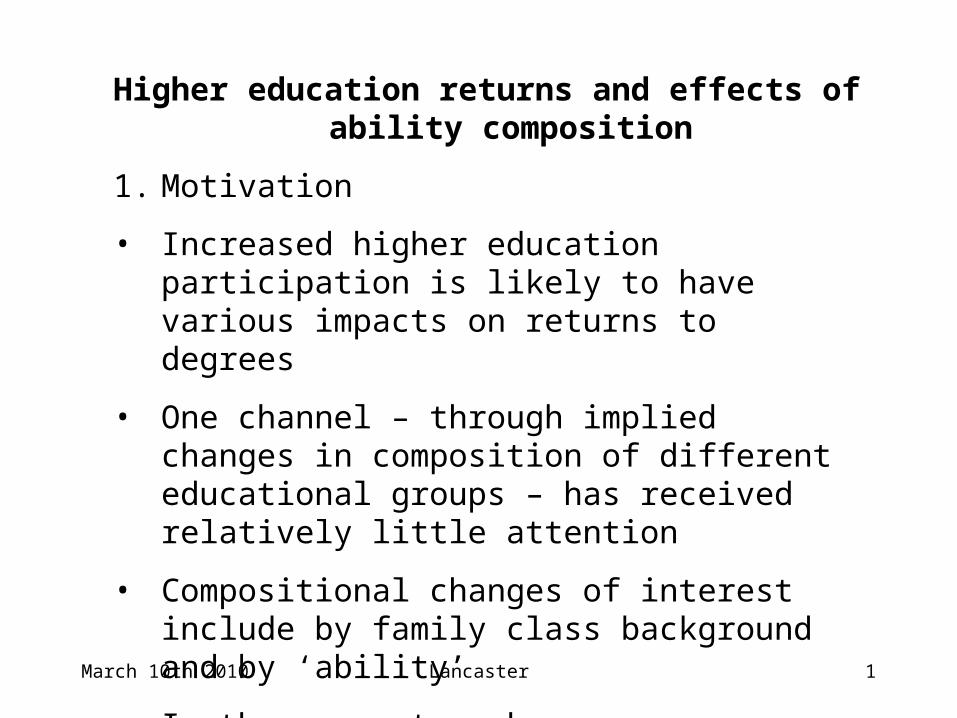
Higher education returns and effects of ability composition

1. Motivation

• Increased higher education participation is likely to have various impacts on returns to degrees

• One channel – through implied changes in composition of different educational groups – has received relatively little attention

• Compositional changes of interest include by family class background and by ‘ability’

• In the current work, we are interested in ability composition


2. Aims

We will focus on:

(i) The college wage premium(ii) Differences in the premium across different groups

- gender- ability

Why gender? Because graduate expansion has been differential by gender.

Why by ability? Because it’s potentially important but often ignored.


3. Context

HE API in UK shows rapid expansion after mid-1980s,

with growth especially dramatic for women.

See Figure 1.


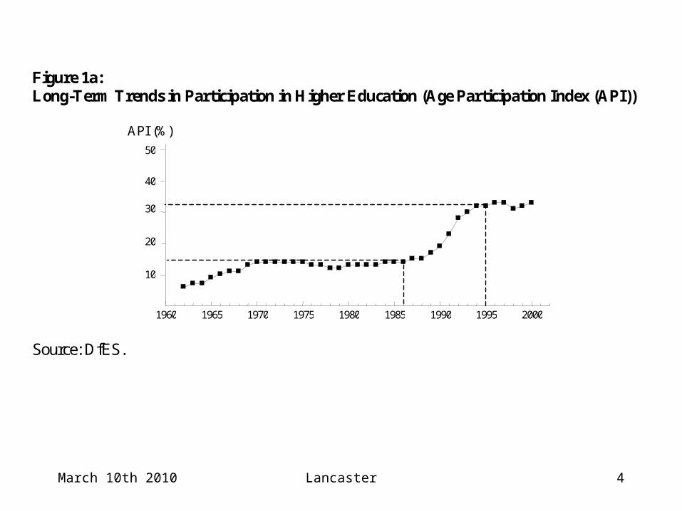
Figure 1a: Long-Term Trends in Participation in Higher Education (Age Participation Index (API))

API (%) Source: DfES.

1960 1965 1970 1975 1980 1985 1990 1995 2000

10

20

30

40

50


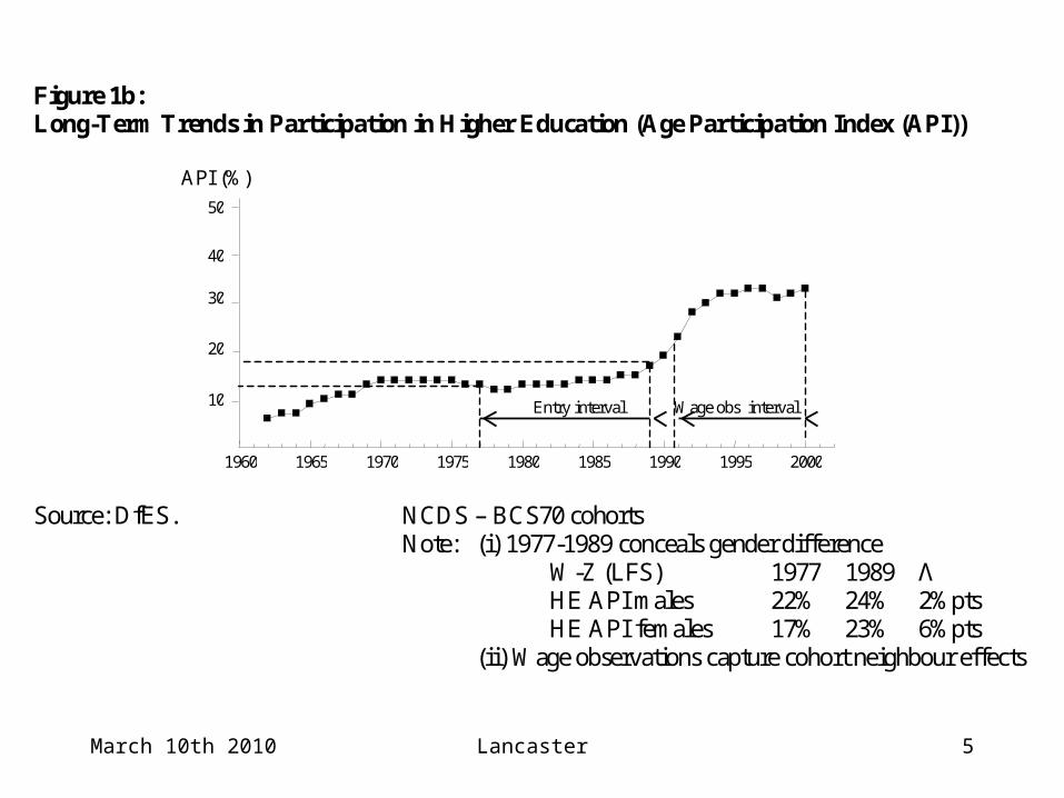
Figure 1b: Long-Term Trends in Participation in Higher Education (Age Participation Index (API))

API (%) Source: DfES. NCDS – BCS70 cohorts Note: (i) 1977-1989 conceals gender difference W-Z (LFS) 1977 1989 Λ

HE API males 22% 24% 2%pts HE API females 17% 23% 6%pts (ii) Wage observations capture cohort neighbour effects

1960 1965 1970 1975 1980 1985 1990 1995 2000

10

20

30

40

50

Entry interval Wage obs interval


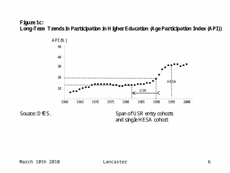
Figure 1c: Long-Term Trends in Participation in Higher Education (Age Participation Index (API))

API (%) Source: DfES. Span of USR entry cohorts and single HESA cohort

1960 1965 1970 1975 1980 1985 1990 1995 2000

10

20

30

40

50

USR

HESA


4. Why did the HE API rise?

Demand-side factors:derived demand (SBTC)GCSE pass rates

Supply-side factors:Increase in places

- finance following student- end of binary divide

Loans system

W-Z: from mid-80s to mid-90s, SS dominated DD factors=> r (specifically, Pg) predicted to fall, cet. par.

s

r

D1D2

S=MC

r

s

S1S2

D=MB


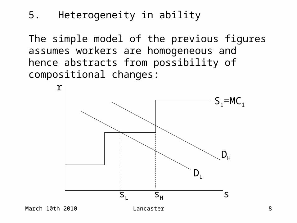
5. Heterogeneity in ability

The simple model of the previous figures assumes workers are homogeneous and hence abstracts from possibility of compositional changes:

ssH

r

S1=MC1

sL

DL

DH


A fall in costs can produce a change in the ability composition:

(similarly, a change in marginal benefits could produce a change in family background composition)

ssL=sH

r

S1=MC1

DL

DH

S2=MC2


At the individual level, the issue of the relationship between ability and educational investments when individuals are heterogeneous is well-known and is associated with the problem of ability bias in estimates of returns to education.

At the macro (cohort) level, cohort changes (eg in participation) can impact on estimates of returns through changes in the extent of ability bias across cohorts.


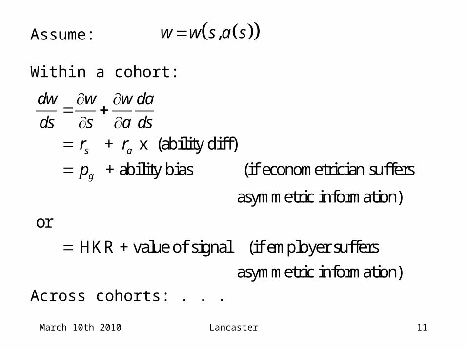
Assume:

Within a cohort:

Across cohorts: . . .

,w w s a s

+ x (ability diff)

+ ability bias (if econometrician suffers

asymmetric information)

or

HK

s a

g

dw w w da

ds s a dsr r

p

R + value of signal (if employer suffers

asymmetric information)


Across cohorts:

can change because of changes in:

(i)

(ii)

(iii)

The literature has focused on (i) and (ii) (see Cawley et al., 2000) .

But see Blackburn and Neumark (1991, 1993, 1995) and R

s

a

dw

dsr

r

da

ds

osenbaum (2003).


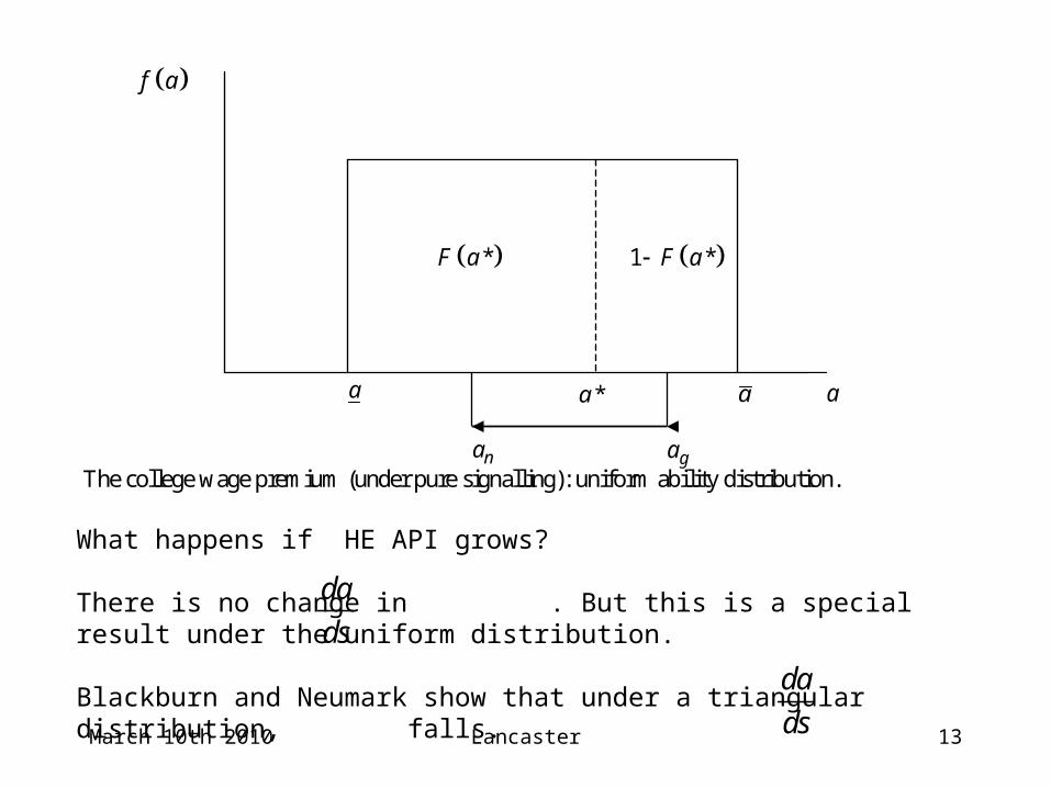
The college wage premium (under pure signalling): uniform ability distribution.

*a a a a

ga na

*F a 1 *F a

f a

What happens if HE API grows? There is no change in . But this is a special result under the uniform distribution.

Blackburn and Neumark show that under a triangular distribution, falls.

da

ds

da

ds


The implication is that graduate expansion over cohorts produces a compositional change of a type that leads to a reduction in ability bias (or a lower value to the signal of a degree), ceteris paribus, and hence a lower estimate of the college wage premium.

The US literature on this was not developed further as the Blackburn-Neumark analysis was attempting to explain an increase in the college wage premium at a time of higher college participation.

Rosenbaum (2003) finds evidence supporting the view that compositional changes can explain longer term patterns in the college wage premium in the US. (See INST: p.11)


6. Evidence on the UK college wage premium over time

(i)Harkness-Machin (1999)pg was rising in the 80s and constant in the 90sLikely explanation: SBTC in 80s raised rs and ra;

offset in 90s by graduate expansion

(ii)Walker-Zhu (2008)(LFS) Focus on birth cohorts of 66-68 vs 75-77 (see

Figure 1a, p. 5): API more than doubled.

Result: pg constant for men (15%) and

pg rising for women (40% -> 47%)

Conclusion: ra must have been rising to offset what must have been falling rs (and compositional changes)


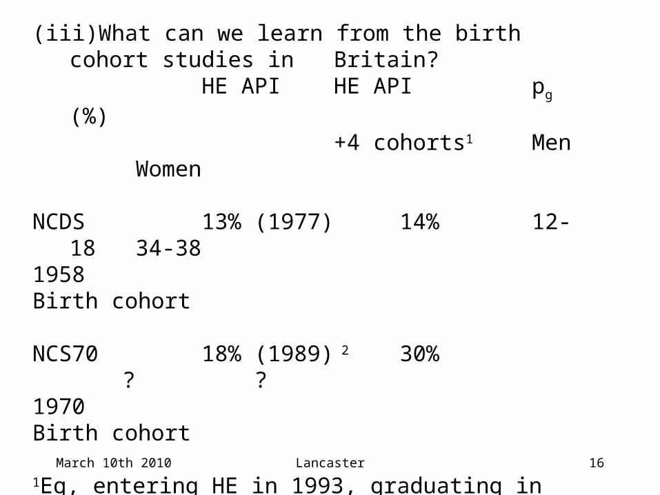
(iii) What can we learn from the birth cohort studies in Britain?

HE API HE API pg (%)+4 cohorts1 Men

Women

NCDS 13% (1977) 14% 12-18 34-381958Birth cohort

NCS70 18% (1989) 2 30% ? ?1970Birth cohort

1Eg, entering HE in 1993, graduating in 1996, 4yrs experience by 2000 when £ observed of 1970 birth cohort.2Conceals extent of growth in female participation in HE.


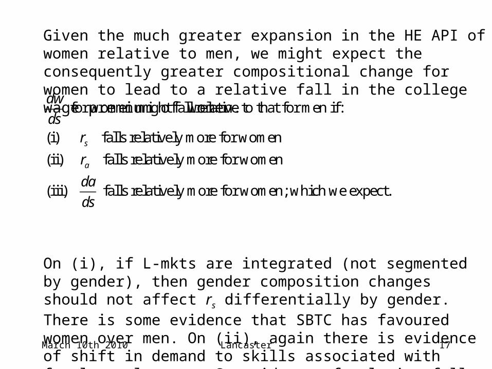
Given the much greater expansion in the HE API of women relative to men, we might expect the consequently greater compositional change for women to lead to a relative fall in the college wage premium of women.

On (i), if L-mkts are integrated (not segmented by gender), then gender composition changes should not affect rs differentially by gender. There is some evidence that SBTC has favoured women over men. On (ii), again there is evidence of shift in demand to skills associated with female employment. So evidence of relative fall in college premium for women would indicate importance of role for (iii).

for women might fall relative to that for men if:

(i) falls relatively more for women

(ii) falls relatively more for women

(iii) falls relatively more for women; which we

s

a

dw

dsr

r

da

dsexpect.


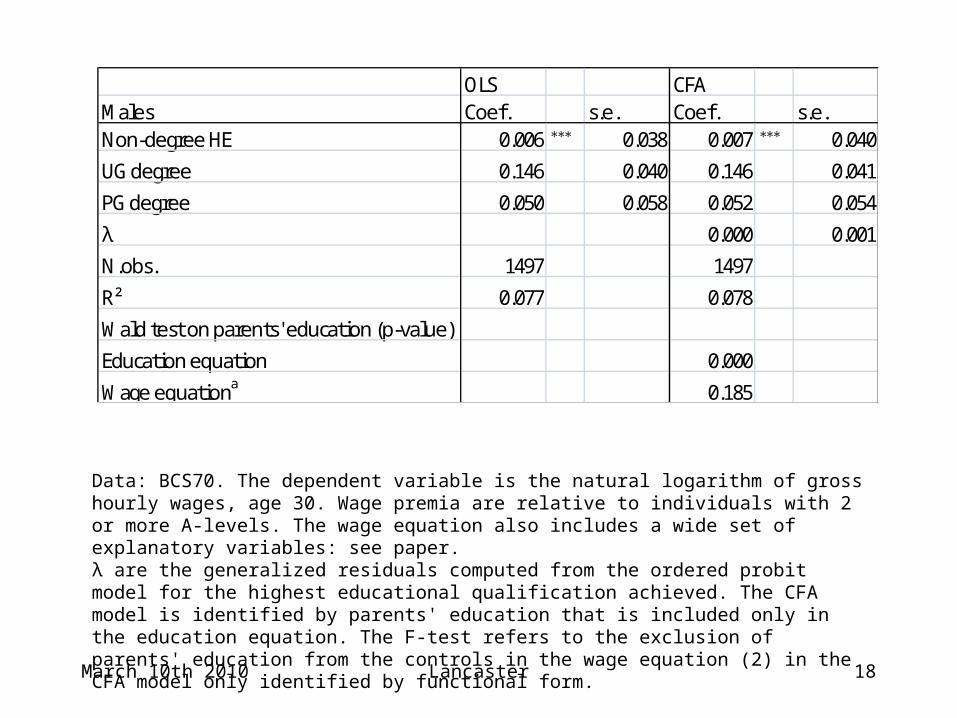
OLS CFAMales Coef. s.e. Coef. s.e.Non-degree HE 0.006 0.038 0.007 0.040

UG degree 0.146

∗∗∗0.040 0.146

∗∗∗0.041

PG degree 0.050 0.058 0.052 0.054

λ 0.000 0.001

N.obs. 1497 1497

R² 0.077 0.078

Wald test on parents' education (p-value)

Education equation 0.000

Wage equationa 0.185

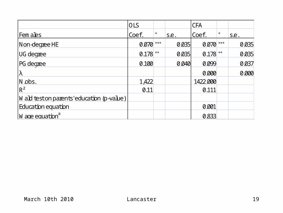
Data: BCS70. The dependent variable is the natural logarithm of gross hourly wages, age 30. Wage premia are relative to individuals with 2 or more A-levels. The wage equation also includes a wide set of explanatory variables: see paper.λ are the generalized residuals computed from the ordered probit model for the highest educational qualification achieved. The CFA model is identified by parents' education that is included only in the education equation. The F-test refers to the exclusion of parents' education from the controls in the wage equation (2) in the CFA model only identified by functional form.


OLS CFA

Females Coef. s.e. Coef. s.e.

Non-degree HE 0.070

∗0.035 0.070

∗0.035

UG degree 0.178

∗∗∗0.035 0.178

∗∗∗0.035

PG degree 0.100

∗∗0.040 0.099

∗∗0.037

λ 0.000 0.000N.obs. 1,422 1422.000R² 0.11 0.111Wald test on parents' education (p-value)Education equation 0.001

Wage equationa 0.833


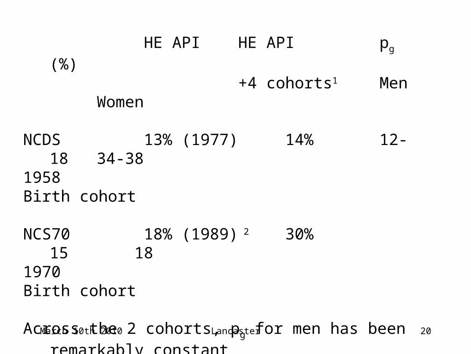
HE API HE API pg (%)+4 cohorts1 Men

Women

NCDS 13% (1977) 14% 12-18 34-381958Birth cohort

NCS70 18% (1989) 2 30% 15 181970Birth cohort

Across the 2 cohorts, pg for men has been remarkably constantwhile pg for women has fallen dramatically, to be similar tothat for men. Supports hypothesis that compositional changesimportant.


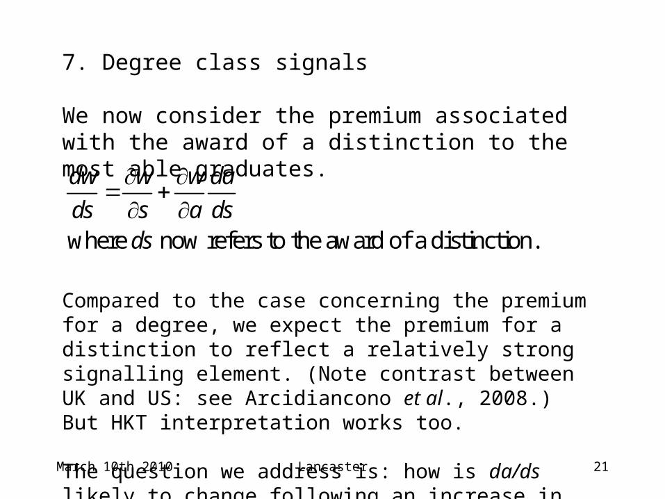
7. Degree class signals

We now consider the premium associated with the award of a distinction to the most able graduates.

Compared to the case concerning the premium for a degree, we expect the premium for a distinction to reflect a relatively strong signalling element. (Note contrast between UK and US: see Arcidiancono et al., 2008.) But HKT interpretation works too.

The question we address is: how is da/ds likely to change following an increase in the HE API?

where now refers to the award of a distinction.

dw w w da

ds s a dsds


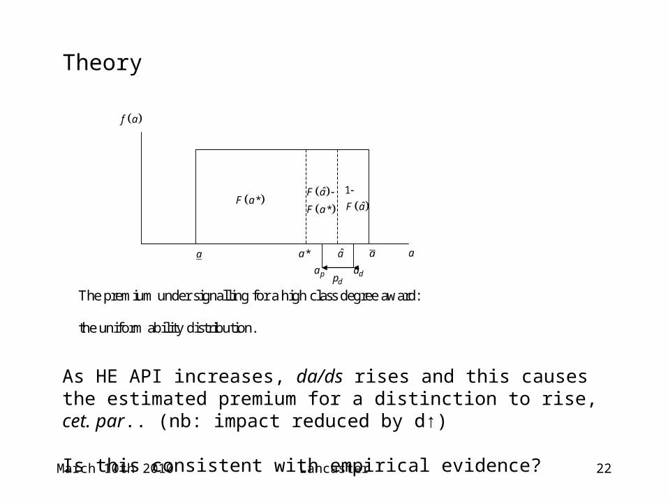
Theory

As HE API increases, da/ds rises and this causes the estimated premium for a distinction to rise, cet. par.. (nb: impact reduced by d↑)

Is this consistent with empirical evidence?

The premium under signalling for a high class degree award:

the uniform ability distribution.

*a a a a

da pa dp

*F a

ˆ

*

F a

F a

a

1

ˆF a

f a


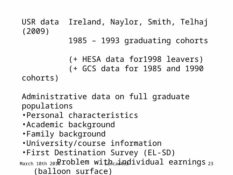
USR data Ireland, Naylor, Smith, Telhaj (2009)1985 – 1993 graduating cohorts (+ HESA data for1998 leavers)(+ GCS data for 1985 and 1990 cohorts)

Administrative data on full graduate populations•Personal characteristics•Academic background•Family background•University/course information•First Destination Survey (EL-SD)

Problem with individual earnings (balloon surface)

Average occupational earnings (averaged over all years)


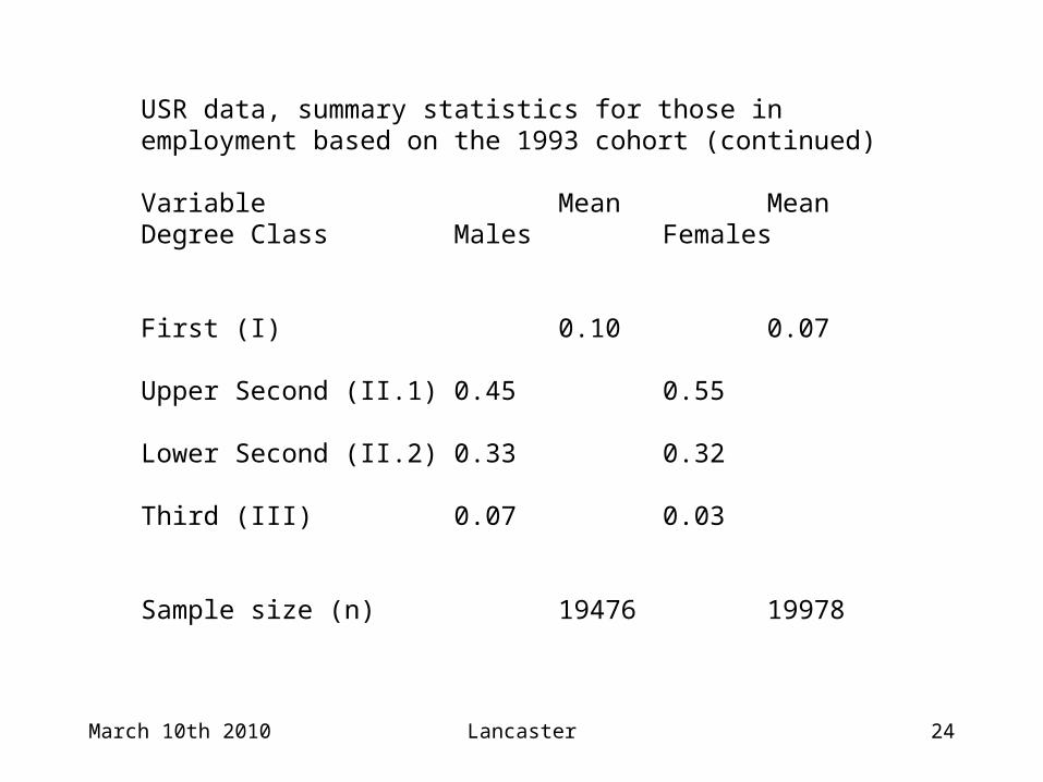
USR data, summary statistics for those in employment based on the 1993 cohort (continued)

Variable Mean MeanDegree Class Males Females

First (I) 0.10 0.07

Upper Second (II.1) 0.45 0.55

Lower Second (II.2) 0.33 0.32

Third (III) 0.07 0.03

Sample size (n) 19476 19978


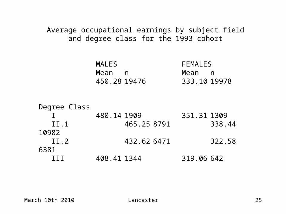
Average occupational earnings by subject field and degree class for the 1993 cohort

MALES FEMALES Mean n Mean n

450.28 19476 333.10 19978

Degree Class I 480.14 1909 351.31 1309 II.1 465.25 8791 338.44 10982 II.2 432.62 6471 322.58 6381 III 408.41 1344 319.06 642


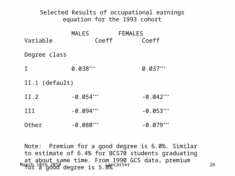
Selected Results of occupational earnings equation for the 1993 cohort

MALES FEMALESVariable Coeff Coeff

Degree class

I 0.038*** 0.037***

II.1 (default)

II.2 -0.054*** -0.042***

III -0.094*** -0.053***

Other -0.080*** -0.079***

Note: Premium for a good degree is 6.0%. Similar to estimate of 6.4% for BCS70 students graduating at about same time. From 1990 GCS data, premium for a good degree is 5.0%


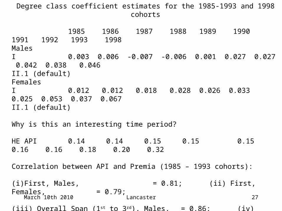
Degree class coefficient estimates for the 1985-1993 and 1998 cohorts

1985 1986 1987 1988 1989 1990 1991 1992 1993 1998 MalesI 0.003 0.006 -0.007 -0.006 0.001 0.027 0.027 0.042 0.038 0.046II.1 (default)FemalesI 0.012 0.012 0.018 0.028 0.026 0.033 0.025 0.053 0.037 0.067II.1 (default)

Why is this an interesting time period?

HE API 0.14 0.14 0.15 0.15 0.15 0.16 0.16 0.18 0.20 0.32

Correlation between API and Premia (1985 – 1993 cohorts):

(i)First, Males, = 0.81; (ii) First, Females, = 0.79;

(iii) Overall Span (1st to 3rd), Males, = 0.86; (iv) Overall Span, Females, = 0.64.

Over this time period, there is no strong evidence of substantial increases in rs or ra: W-Z show degree returns constant for both men and women at least prior to 1995 graduates.

Documents

March 10th 2010Lancaster1 Higher education returns and effects of ability composition 1.Motivation Increased higher education participation is likely to