Embed Size (px)
Citation preview
Market Equilibrium Analysis Considering ElectricVehicle Aggregators and Wind Power Producers
Without Storage Capabilities
Oscar Andres Dıaz Caballero
University of Los Andes
School of Engineering, Department of Electrical and Electronic Engineering
Bogota, Colombia
2019


Market Equilibrium Analysis Considering ElectricVehicle Aggregators and Wind Power Producers
Without Storage Capabilities
Oscar Andres Dıaz Caballero
University of Los Andes
Submitted in partial fulfillment of the requirements for the degree of:
Electrical engineer
Advisor:
Prof. Paulo Manuel De Oliveira De Jesus
Degree work defended on:
June 6, 2019 - 2:00 pm
University of Los Andes
Faculty of Engineering, Department of Electrical and Electronic Engineering
Bogota, Colombia
2019


Acknowledgements
In first place I’m grateful with my parents Oscar
Dıaz and Celia Teresa and my brother Daniel
Felipe, my greatest support in this journey that
some people like to call life. You’ve made me
who I am today.
In second place, professor Paulo, thank you for
your accompaniment and contributions in this
project.
And last but not least to all my friends, espe-
cially Paula Galvis, my best friend and one of
the best people I’ve ever met. You’ve made this
journey an unique experience that I will never
forget.


vii
Abstract
This document is devoted to analyze market equilibrium solutions when new market agents,
such as renewable/intermittent producers, elastic demands and electric vehicles, are exposed
to time-varying Locational Marginal Prices in the context of a competitive electricity market.
We consider three main features for these market agents:
1. Load demands are deemed to be elastic, being fully responsive to price changes
2. Renewable-based producers, such as wind farms are not dispatchable in real power and
deprived of storage capabilities.
3. Electric-vehicle retailers –defined as EV aggregators– are able to manage charge-
discharge pattern of EV’s batteries in order to enhance daily profits due to energy
traded in the wholesale electricity market.
After a brief discussion about different economic equilibrium models in power systems (Per-
fect competition, Nash-Cournot, Stackelberg and Monopoly), two economic equilibrium mo-
dels are studied in detail. First, we analyze the perfect competition solution driven by a
benevolent planner in which real and reactive power dispatches as well as the battery charge-
discharge schedule aims to maximize the global social welfare. Secondly, we also address the
monopolistic solution where the total profit of EV aggregators and renewable generators are
maximized considering that both producers belong to the same firm.
Solutions were obtained using a multi-period alternating current optimal power flow (AC-
OPF) formulation in which nodal reactive power injections can be modified by renewable
generators and EV aggregators in order to shift the locational marginal prices to their own
benefit. The 24-hour AC-OPF was stated as the maximization problem subject to active and
reactive power equilibrium equations as well as battery capacity constraints.
The perfect competition and monopolistic system models were applied to an illustrative
3-node test system. Optimization problems were solved using MATLAB’s fmincon optimi-
zation tool.
Keywords: Optimal Power Flow, Social Welfare, Optimization, Monopolistic, Nash Equilibrium,
Stackelberg Game, Locational Marginal Prices, Wind Power, EV Aggregator.
Table of Contents
List of Figures X
List of Tables XI
1. Introduction 1
1.1. Objectives . . . . . . . . . . . . . . . . . . . . . . . . . . . . . . . . . . . . . 3
1.1.1. General . . . . . . . . . . . . . . . . . . . . . . . . . . . . . . . . . . 3
1.1.2. Specific . . . . . . . . . . . . . . . . . . . . . . . . . . . . . . . . . . 3
2. Theoretical Framework 4
2.1. Background . . . . . . . . . . . . . . . . . . . . . . . . . . . . . . . . . . . . 4
2.2. Optimal Power Flow for Minimal Losses . . . . . . . . . . . . . . . . . . . . 5
2.3. The AC Network Model . . . . . . . . . . . . . . . . . . . . . . . . . . . . . 5
2.4. Locational Marginal Prices structure . . . . . . . . . . . . . . . . . . . . . . 7
2.4.1. The system Lambda . . . . . . . . . . . . . . . . . . . . . . . . . . . 7
2.4.2. Incremental losses . . . . . . . . . . . . . . . . . . . . . . . . . . . . . 7
2.5. Social Welfare concept . . . . . . . . . . . . . . . . . . . . . . . . . . . . . . 9
2.6. Energy Storage Model - 24 Hours Power Flow . . . . . . . . . . . . . . . . . 12
2.7. Optimization approach . . . . . . . . . . . . . . . . . . . . . . . . . . . . . . 13
3. Market equilibrium in power systems without network and storage constraints 14
3.1. Monopolistic Solution . . . . . . . . . . . . . . . . . . . . . . . . . . . . . . . 14
3.2. Nash-Cournot Equilibrium . . . . . . . . . . . . . . . . . . . . . . . . . . . . 15
3.3. Stackelberg Equilibrium . . . . . . . . . . . . . . . . . . . . . . . . . . . . . 15
3.4. Perfect Competition . . . . . . . . . . . . . . . . . . . . . . . . . . . . . . . 15
3.5. Comparison analysis . . . . . . . . . . . . . . . . . . . . . . . . . . . . . . . 16
4. Market equilibrium in power systems with network and storage constraints 18
4.1. Network Model and Constraints . . . . . . . . . . . . . . . . . . . . . . . . . 18
4.2. Optimal Power Flow Problem . . . . . . . . . . . . . . . . . . . . . . . . . . 18
4.2.1. Minimum Losses Dispatch . . . . . . . . . . . . . . . . . . . . . . . . 19
4.2.2. Maximum Social Welfare (Perfect Competition) . . . . . . . . . . . . 19
4.2.3. Monopoly Equilibrium . . . . . . . . . . . . . . . . . . . . . . . . . . 20
4.3. Analysis and Comparison Procedure . . . . . . . . . . . . . . . . . . . . . . 21

Table of Contents ix
5. Study case 23
5.1. Three node example . . . . . . . . . . . . . . . . . . . . . . . . . . . . . . . 23
5.1.1. Wind power curve . . . . . . . . . . . . . . . . . . . . . . . . . . . . 24
5.1.2. Elastic and inelastic demand . . . . . . . . . . . . . . . . . . . . . . . 24
5.1.3. Spot market price (λ0) . . . . . . . . . . . . . . . . . . . . . . . . . . 25
5.1.4. System matrix (YBUS) . . . . . . . . . . . . . . . . . . . . . . . . . . 25
5.1.5. Operational limits . . . . . . . . . . . . . . . . . . . . . . . . . . . . . 26
6. Results 27
6.1. Minimum losses equilibrium . . . . . . . . . . . . . . . . . . . . . . . . . . . 27
6.2. Perfect competition . . . . . . . . . . . . . . . . . . . . . . . . . . . . . . . . 29
6.3. Monopoly scenario . . . . . . . . . . . . . . . . . . . . . . . . . . . . . . . . 30
6.4. Market comparison for the 3 scenarios . . . . . . . . . . . . . . . . . . . . . 31
6.5. Comparison of scenario variations . . . . . . . . . . . . . . . . . . . . . . . . 32
6.5.1. Maximum social welfare . . . . . . . . . . . . . . . . . . . . . . . . . 32
6.5.2. Monopoly . . . . . . . . . . . . . . . . . . . . . . . . . . . . . . . . . 33
7. Conclusions and recommendations 35
7.1. Conclusions . . . . . . . . . . . . . . . . . . . . . . . . . . . . . . . . . . . . 35
7.2. Recommendations and future work . . . . . . . . . . . . . . . . . . . . . . . 36
Bibliography 36
A. Annexes 40
A.1. Annex 1: Market Equilibrium Solutions . . . . . . . . . . . . . . . . . . . . . 40
A.1.1. Producers and Demand Model . . . . . . . . . . . . . . . . . . . . . . 40
A.1.2. Perfect competition equilibrium . . . . . . . . . . . . . . . . . . . . . 40
A.1.3. Monopoly equilibrium . . . . . . . . . . . . . . . . . . . . . . . . . . 41
A.1.4. Regulatory Solution . . . . . . . . . . . . . . . . . . . . . . . . . . . . 42
A.1.5. Nash-Cournot equilibrium: Duopoly . . . . . . . . . . . . . . . . . . . 42
A.1.6. Stackelberg equilibrium . . . . . . . . . . . . . . . . . . . . . . . . . . 43
A.1.7. Equilibrium Example: 2 Producers with Elastic Demand . . . . . . . 43
A.2. Annex 2: Symbols and Acronyms . . . . . . . . . . . . . . . . . . . . . . . . 45

List of Figures
2-1. Elastic demand example . . . . . . . . . . . . . . . . . . . . . . . . . . . . . 10
2-2. 24 hours power dispatch . . . . . . . . . . . . . . . . . . . . . . . . . . . . . 12
2-3. MATLAB interior-point algorithm . . . . . . . . . . . . . . . . . . . . . . . . 13
3-1. Example of perfect competition in a market . . . . . . . . . . . . . . . . . . 16
3-2. Equilibrium solutions for a simple example . . . . . . . . . . . . . . . . . . . 17
5-1. System model used for the optimization . . . . . . . . . . . . . . . . . . . . . 23
5-2. Wind farm power curve . . . . . . . . . . . . . . . . . . . . . . . . . . . . . . 24
5-3. Demand curves for elastic and inelastic case . . . . . . . . . . . . . . . . . . 24
5-4. Spot price curve for 24 hours . . . . . . . . . . . . . . . . . . . . . . . . . . . 25
6-1. System status: Minimum Losses OPF . . . . . . . . . . . . . . . . . . . . . . 27
6-2. System Line Flows: Minimum Losses . . . . . . . . . . . . . . . . . . . . . . 28
6-3. Nodal Prices and System Losses: Minimum Losses . . . . . . . . . . . . . . . 28
6-4. System status: Maximum SW . . . . . . . . . . . . . . . . . . . . . . . . . . 29
6-5. System Line Flows: Maximum SW . . . . . . . . . . . . . . . . . . . . . . . 30
6-6. Nodal Prices and System Losses: Maximum SW . . . . . . . . . . . . . . . . 30
6-7. System status: Maximum π2 + π3 . . . . . . . . . . . . . . . . . . . . . . . . 30
6-8. System Line Flows: Maximum π2 + π3 . . . . . . . . . . . . . . . . . . . . . 31
6-9. Nodal Prices and System Losses: Maximum π2 + π3 . . . . . . . . . . . . . . 31
A-1. Equilibrium solutions for the example (demand) . . . . . . . . . . . . . . . . 44
List of Tables
2-1. Background in optimal power flow with network and storage constraints . . . 4
5-1. Limits for the system variables . . . . . . . . . . . . . . . . . . . . . . . . . . 26
6-1. Comparative table for the 3 optimization methods . . . . . . . . . . . . . . . 31
6-2. Comparative table for the 3 optimization methods (LMP) . . . . . . . . . . 32
6-3. Scenarios for line limits . . . . . . . . . . . . . . . . . . . . . . . . . . . . . . 32
6-4. Comparative table for scenario variations - SW . . . . . . . . . . . . . . . . 33
6-5. Comparative table for scenario variations (LMP) - SW . . . . . . . . . . . . 33
6-6. Comparative table for scenario variations - Monopoly . . . . . . . . . . . . . 33
6-7. Comparative table for scenario variations (LMP) - Monopoly . . . . . . . . . 34
A-1. Comparison between the studied equilibrium . . . . . . . . . . . . . . . . . . 44
A-2. Comparison between the studied equilibrium (producers and SW) . . . . . . 45
A-3. Symbols and Acronyms . . . . . . . . . . . . . . . . . . . . . . . . . . . . . . 45
1. Introduction
In the scope of Smart Grid paradigm [Huang et al., 2012], we can identify that ongoing po-
wer system modernization process is carried out applying four main drivers: 1) energy matrix
transformation by allocating large amounts of renewable energy, 2) promoting electric mo-
bility in order to substitute combustion engines in the transportation sector, 3) widespread
deployment of smart meters in order to apply demand-response programs, and 4) the de-
ployment of Advanced Metering Infrastructure (AMI) enables the application of real-time
pricing schemes to market agents due to their impact on energy losses and congestion.
Renewable energies are being progressively introduced to the electricity market in the last
few years boosted by national police-making energy diversification goals and increasing envi-
ronmental concerns [Herig, 2003]. Several markets around the world have included renewable
resources in their portfolio in spite of the increase in variability and therefore the undesirable
effects on system reliability. Thus, since intermittent sources produce energy proportionally
with wind speed and solar irradiance, which cannot be turned off or adjusted, they must be
regarded as non-dispatchable in real power. As a result, intermittent renewable generation
is capable to provide reliable energy to the market since forecasting models have reached
certain maturity but with capacity limitations with respect to centralized generation. To
solve this drawback, energy storage devices such as batteries can be included in renewable
plants. As this solution implies an increased capital expenditure (CAPEX), renewable energy
promoters are installing generation facilities without storage capabilities [Root et al., 2017].
Generalized electric mobility have important energy storage capabilities that intermittent
sources do not have. Thus, electric vehicle (EV) aggregators can provide capacity and energy
as virtual power producers by exploiting business opportunities trading part of the stored
energy in the plug-in vehicles in the wholesale electricity market [Artakusuma et al., 2014].
Under a 24-hour cycle, EV aggregators can decide when and how to charge and discharge
the batteries in order to maximize their own profit and transferring part of these benefits to
the EV owners. In addition to this, EV aggregators and renewable producers can manage
reactive power via power electronics or other reactive power compensation devices.
Smart metering can enable sending energy prices to elastic consumers under a real time-
basis. In this case, retail aggregators can seek savings by managing demand profiles taking
into account price changes. Real-time prices can be sent to users using locational informa-
2 1 Introduction
tion, accounting not only the cost of electricity in the wholesale markets but also the effects
upon losses and line congestion [Negash and Kirschen, 2014].
Under advanced smart grid paradigm with telemetry based upon Phasor Measurement Units
(PMU), Distribution Management System applications such as State Estimation and Opti-
mal Power Flow are capable to compute Locational Marginal Prices (LMP) and send them
to market agents using the Advanced Metering Infrastructure (AMI) [Heydt et al., 2012]
These new features will affect the structure of electricity markets. Traditionally, if the cost
structure of a electricity market is known, the market equilibrium points (perfect competi-
tion, oligopolistic or monopolistic solution) can be emulated using the Optimal Power Flow
tool (either DC or AC formulation) where the marginal prices are acquired by computing
the corresponding Lagrange multipliers. There are several approaches to analyze electri-
city markets from the OPF perspective: Security Economic Dispatch, Security Constrained
OPF, Hydrothermal coordination, etc [Zhu, 2015]. The research question raised here is how
to evaluate market equilibria (perfect competition and monopolistic solutions) when above
mentioned market agents –with and without storage capabilities– are included in the formu-
lation of the complete AC optimal power flow.
After a brief discussion about different economic equilibrium models in power systems
(Perfect competition, Nash-Cournot, Stackelberg and Monopoly), two economic equilibrium
models are studied in detail. First, we analyze the perfect competition solution driven by
a benevolent planner in which real and reactive power dispatches as well as the battery
charge-discharge schedule aims to maximize the global social welfare. Secondly, we address
the monopolistic solution where the total profit of EV aggregators and renewable genera-
tors are maximized considering that both producers belong to the same firm. Both market
equilibrium approaches are analyzed and compared with a minimum loss solution dispatch
performed by the operator. The 24-hour AC-OPF was stated as the maximization problem
subject to active and reactive power equilibrium equations as well as battery capacity cons-
traints.
The paper is structured as follows: 1) Introduction, 2) Theoretical Framework, 4) Mar-
ket equilibrium in power systems with network and storage constraints, 5) Study case, 6)
Results, 7) Conclusions and recommendations, A.1) Annex 1: Market Equilibrium Solutions,
A.2) Annex 2: Symbols and Acronyms.

1.1 Objectives 3
1.1. Objectives
1.1.1. General
Formulate and solve the AC Optimal Power Flow problem for different market equilibrium
points –Minimum Losses, Perfect Competition and Monopoly– considering three agents ex-
posed to Locational Marginal Prices: Elastic demands, Renewable (Wind) producer without
storage capabilities and Electric Vehicle aggregators.
1.1.2. Specific
Discuss perfect competition and monopoly market equilibrium points in traditional
power systems without network and storage constraints.
Apply the AC-OPF formulations for perfect competition and monopoly equilibria in
an illustrative 3-node power system, under a 24-hour dispatch strategy.
Perform a comparison and analysis of the obtained solutions.
2. Theoretical Framework
2.1. Background
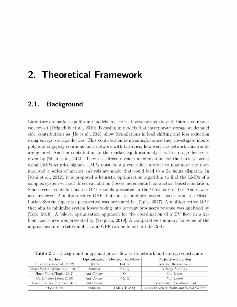
Literature on market equilibrium models in electrical power system is vast. Interested reader
can revisit [Delgadillo et al., 2010]. Focusing in models that incorporate storage at demand
side, contributions as [He et al., 2015] show formulations in load shifting and loss reduction
using energy storage devices. This contribution is meaningful since they investigate mono-
poly and oligopoly solutions for a network with batteries; however, the network constraints
are ignored. Another contribution to the market equilibria analysis with storage devices is
given by [Zhao et al., 2014]. They use direct revenue maximization for the battery owner
using LMPs as price signals. LMPs must be a given value in order to maximize the reve-
nue, and a series of market analysis are made that could lead to a 24 hours dispatch. In
[Vani et al., 2012], it is proposed a heuristic optimization algorithm to find the LMPs of a
complex system without direct calculation (losses incremental) nor auction-based simulation.
Some recent contributions on OPF models presented in the University of Los Andes were
also reviewed. A multiobjective OPF that aim to minimize system losses from the Distri-
bution System Operator perspective was presented in [Tapia, 2017]. A multiobjective OPF
that aim to minimize system losses taking into account producers revenue was analyzed by
[Toro, 2018]. A bilevel optimization approach for the coordination of a EV fleet in a 24-
hour load curve was presented by [Toquica, 2019]. A comparative summary for some of the
approaches to market equilibria and OPF can be found in table 2-1.
Table 2-1.: Background in optimal power flow with network and storage constraintsAuthor Optimization Decision variables Objective Function
S. Vani [Vani et al., 2012] BFOA LMPs Auction Replacement
Majid Wafaa [Wafaa et al., 2016] fmincon P & Q Voltage Stability
Hugo Tapia [Tapia, 2017] Ant Colony Q Min Losses
Carlos Toro [Toro, 2018] Ant Colony P & Q Min Losses
David Toquica [Toquica, 2019] Ant Colony P EV revenue Operational cost
Oscar Dıaz fmincon LMPs, P & Q Losses Producer Profit and Social Welfare
2.2 Optimal Power Flow for Minimal Losses 5
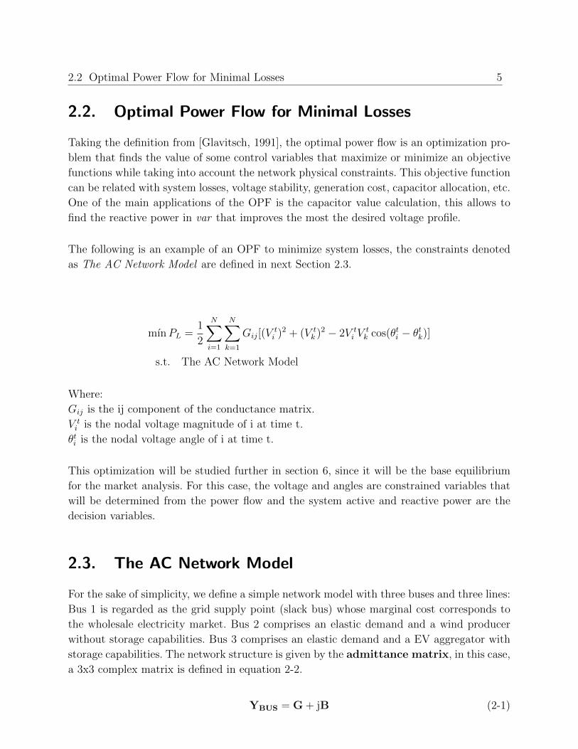
2.2. Optimal Power Flow for Minimal Losses
Taking the definition from [Glavitsch, 1991], the optimal power flow is an optimization pro-
blem that finds the value of some control variables that maximize or minimize an objective
functions while taking into account the network physical constraints. This objective function
can be related with system losses, voltage stability, generation cost, capacitor allocation, etc.
One of the main applications of the OPF is the capacitor value calculation, this allows to
find the reactive power in var that improves the most the desired voltage profile.
The following is an example of an OPF to minimize system losses, the constraints denoted
as The AC Network Model are defined in next Section 2.3.
mınPL =1
2
N∑i=1
N∑k=1
Gij[(Vti )2 + (V t
k )2 − 2V ti V
tk cos(θti − θtk)]
s.t. The AC Network Model
Where:
Gij is the ij component of the conductance matrix.
V ti is the nodal voltage magnitude of i at time t.
θti is the nodal voltage angle of i at time t.
This optimization will be studied further in section 6, since it will be the base equilibrium
for the market analysis. For this case, the voltage and angles are constrained variables that
will be determined from the power flow and the system active and reactive power are the
decision variables.
2.3. The AC Network Model
For the sake of simplicity, we define a simple network model with three buses and three lines:
Bus 1 is regarded as the grid supply point (slack bus) whose marginal cost corresponds to
the wholesale electricity market. Bus 2 comprises an elastic demand and a wind producer
without storage capabilities. Bus 3 comprises an elastic demand and a EV aggregator with
storage capabilities. The network structure is given by the admittance matrix, in this case,
a 3x3 complex matrix is defined in equation 2-2.
YBUS = G + jB (2-1)
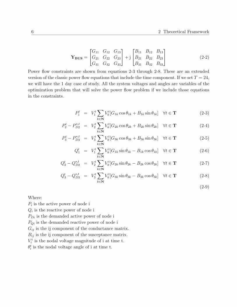
6 2 Theoretical Framework
YBUS =
G11 G12 G13
G21 G22 G23
G31 G32 G33
+ j
B11 B12 B13
B21 B22 B23
B31 B32 B33
(2-2)
Power flow constraints are shown from equations 2-3 through 2-8. These are an extended
version of the classic power flow equations that include the time component. If we set T = 24,
we will have the 1 day case of study. All the system voltages and angles are variables of the
optimization problem that will solve the power flow problem if we include those equations
in the constraints.
P t1 = V t
1
∑k∈N
V tk [G1k cos θ1k +B1k sin θ1k] ∀t ∈ T (2-3)
P t2 − P
∗,tD2 = V t
2
∑k∈N
V tk [G2k cos θ2k +B2k sin θ2k] ∀t ∈ T (2-4)
P t3 − P
∗,tD3 = V t
3
∑k∈N
V tk [G3k cos θ3k +B3k sin θ3k] ∀t ∈ T (2-5)
Qt1 = V t
1
∑k∈N
V tk [G1k sin θ1k −B1k cos θ1k] ∀t ∈ T (2-6)
Qt2 −Q
∗,tD2 = V t
2
∑k∈N
V tk [G2k sin θ2k −B2k cos θ2k] ∀t ∈ T (2-7)
Qt3 −Q
∗,tD3 = V t
3
∑k∈N
V tk [G3k sin θ3k −B3k cos θ3k] ∀t ∈ T (2-8)
(2-9)
Where:
Pi is the active power of node i
Qi is the reactive power of node i
PDi is the demanded active power of node i
PQi is the demanded reactive power of node i
Gij is the ij component of the conductance matrix.
Bij is the ij component of the susceptance matrix.
V ti is the nodal voltage magnitude of i at time t.
θti is the nodal voltage angle of i at time t.

2.4 Locational Marginal Prices structure 7
2.4. Locational Marginal Prices structure
The locational marginal prices (LMP) at given time t=1,...24 and node i=1,2.3 have three
components: the system lambda, the incremental loss factor and the congestion fee:
λti = λ0(1− ηti) + µti (2-10)
Where:
λ0 is the base marginal price
ηti is the incremental losses factor
µti is the incremental congestion factor
In the following, we define each component:
2.4.1. The system Lambda
As said before, Local Marginal Prices can be decomposed in three main components: the
system marginal price, the marginal loss component and the congestion fee. The last one
is one of the main tools for the companies to take advantage from the network constraints,
therefore it will be considered in the model. Taking the definition from [PJM, 2017], the con-
gestion fee represents price of congestion for binding constraints and is calculated using the
Shadow Price. Since it relies in the network constraints to be non-zero, it cannot be defined
in a lossless model. Companies can use this fee strategically to create congestion in the grid
and increase the Local Marginal Price of their node if they have enough power market to do it.
In order to calculate the Local Marginal Prices that have been defined, several approxima-
tions can be made. The traditional approach uses the Lagrange multipliers from the minimum
losses optimization in order to calculate the change in system losses due to the change in
injected power, this approach is described in equation 2-11. Another approximation implies
that all the demands in the system are modeled as elastic, creating the Local Marginal Prices
by the equilibrium between supply and demand.
For the purpose of this work, we consider the 24-hour marginal price profile obtained in the
day ahead market as the system lambda.
2.4.2. Incremental losses
Usually, power systems calculate the Local Marginal Prices using the incremental value of
the losses and the congestion penalty. To calculate the incremental losses value, a process
following the chain rule as in [Mutale et al., 2000] can be made. This calculation only works

8 2 Theoretical Framework
in small systems, since complex calculations have to be made if the Ybus matrix is too complex.
Such values can be found by the following relationship:
ηt2ηt3γt2γt3
=
∂P t2
∂θt2
∂P t3
∂θt2
∂Qt2
∂θt2
∂Qt3
∂θt2∂P t
2
∂θt3
∂P t3
∂θt3
∂Qt2
∂θt3
∂Qt3
∂θt3∂P t
2
∂V t2
∂P t3
∂V t2
∂Qt2
∂V t2
∂Qt3
∂V t2
∂P t2
∂V t3
∂P t3
∂V t3
∂Qt2
∂V t3
∂Qt3
∂V t3
−1
∂Lt
∂θt2∂Lt
∂θt3∂Lt
∂V t2
∂Lt
∂V t3
(2-11)
Entries of the inverse of Jacobian and the right-hand vector are obtained from the partial
derivatives using expressions:
∂P ti
∂θtk= V t
i Vtk [Gik sin(θti − θtk)−Bik cos(θti − θtk)] (2-12)
∂P ti
∂θti= −Bii(V
ti )2 −
3∑k=1
V ti V
tk [Gik sin(θti − θtk)−Bik cos(θti − θtk)] (2-13)
∂P ti
∂V tk
= V ti [Gik cos(θti − θtk) +Bik sin(θti − θtk)] (2-14)
∂P ti
∂V ti
= GiiVti +
3∑k=1
V tk [Gik cos(θti − θtk) +Bik sin(θti − θtk)] (2-15)
∂Qti
∂θtk= −V t
i Vtk [Gik cos(θti − θtk) +Bik sin(θti − θtk)] (2-16)
∂Qti
∂θti= −Gii(V
ti )2 +
3∑k=1
V ti V
tk [Gik cos(θti − θtk) +Bik sin(θti − θtk)] (2-17)
∂Qti
∂V tk
= V ti [Gik sin(θti − θtk)−Bik cos(θti − θtk)] (2-18)
∂Qti
∂V ti
= −BiiVti +
3∑k=1
V tk [Gik sin(θti − θtk)−Bik cos(θti − θtk)] (2-19)
∂Lt
∂θti= 2
3∑k=1
V ti V
tkGik sin(θti − θtk) (2-20)
∂Lt
∂V ti
= 2
3∑k=1
Gik[V ti − V t
k cos(θti − θtk)] (2-21)
Where:
Pi is the active power of node i
Qi is the reactive power of node i
PDi is the demanded active power of node i
2.5 Social Welfare concept 9
PQi is the demanded reactive power of node i
Gij is the ij component of the conductance matrix.
Bij is the ij component of the susceptance matrix.
V ti is the nodal voltage magnitude of i at time t.
θti is the nodal voltage angle of i at time t.
ηt2 is the active incremental value for time t.
γt2 is the reactive incremental value for time t.
Lt are the losses at time t.
Incremental values will be used to calculate the prices in the base methodology (minimum
losses), since for that base case the demand will be assumed as inelastic. Afterwards, the
demand will be assumed as elastic, which allows the Local Marginal Prices to be calculated
from market equilibria between the demand and generation cost curves.
2.5. Social Welfare concept
The introduction of smart meters and Advanced Measuring Infrastructure (AMI) in the de-
mand side of the grid is allowing a demand response originated by price signals. According to
[Barai et al., 2015], a smart meter is a device that includes sophisticated measurement and
calculation hardware, software, calibration and communication capabilities. For interopera-
bility within a smart grid infrastructure, smart meters are designed to perform functions,
and store and communicate data according to certain standards.
Variation of power consumption on the demand side often include demand curtailment pro-
grams and price responsive demand programs. [Qinwei Duan, 2016] This means that the
Independent System Operator, or other administrative roles, can have complete telemetry
of the distribution network and send price signals to the consumers in real time in order to
increase the reliability and efficiency of the power system. Advance Measuring Infrastructure
and phasor Measurement Units can even allow the operator to build a complete Ybus matrix
of the system and run real-time simulations like the ones studied in this paper.
10 2 Theoretical Framework
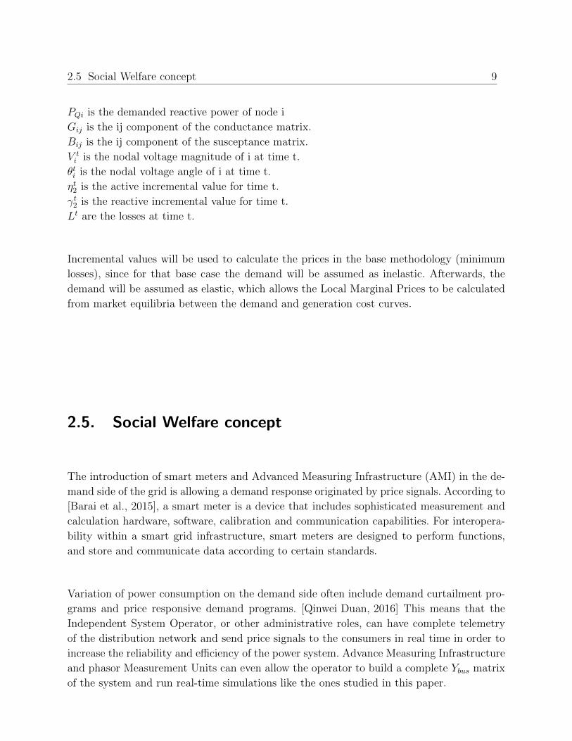
Figure 2-1.: Elastic demand example
Based on the growing demand response programs, it makes sense to model the demand side
load as an elastic demand curve. An example of decreasing curve that can model demand in
an electric system is depicted in figure 2-1. This curves follow the mathematical relationship
stated below. Where λi is the Local Marginal Price, λmaxi is the higher price that the demand
is willing to pay (price for 0 units sold), md is the curve slope and xd is the amount of units
sold.
λi = λmaxi − (Pdi) ·mdi (2-22)
By the means of the previous concepts, we could define the social welfare as any service or
activity designed to promote the welfare of the community and the individual, as through
counseling services. [Barker et al., 2003] Its mathematical definitions is denoted as consu-
mers’ plus producers’ surplus and is a way of representing the total benefit that the society
is receiving from a goods exchange. This definition can be seen below:
SW = Demand Utility - Producer costs (2-23)
SW =N∑i=2
[λmaxi P t
di −mdiP
tdi2
2
]−
N∑i=2
[λmini P t
gi −mgiP
tgi2
2
]− λt1P t
1 (2-24)
(2-25)
Where:
Node 1 is the slack.
λti is the Local Marginal Price for i at time t.
λmaxi is the price intercept for the demand function.

2.5 Social Welfare concept 11
mdi is the slope of the demand function.
moi is the slope of the supply function.
Pdi is the demanded power of node i.
Pgi is the generated power of node i.
Some additional concepts that might be useful to complement this definitions are shown
below:
Consumer marginal benefit: Maximum price that a consumer is willing to pay for
an additional unit of the good that is being consumed.
Consumer marginal utility: Is the satisfaction (in terms of welfare) that a consumer
would receive if an additional unit of the good is consumed.
Generator total cost function: Represents all the costs that a generator would
incur if the production of energy is set to a specific point. It is usually represented as
follows:
Ci(Pgi) = γi + αiPgi +1
2βiP
2gi
Where:
Ci: Total costs of generation.
Pdi: Power output of the generator.
γi: Fixed generation costs.
αi: Linear marginal coefficient.
βi: Quadratic marginal coefficient.
Generator marginal cost function: It is defined as the derivative of the total cost
function and represents the cost of an increase in 1 unit of the power generated. It is
usually represented as follows:
ci(Pdi) = αi + βiPdi
Where:
ci: Marginal costs of generation.
Pdi: Power output of the generator.
αi: Linear marginal coefficient.
βi: Quadratic marginal coefficient.

12 2 Theoretical Framework
2.6. Energy Storage Model - 24 Hours Power Flow
To include the time-related effect of the energy storage device in the grid, it is necessary to
run a dynamic power flow. This means that each variable will have T states per run and
some relationship between states must be made. In this case, the battery state of charge
will be related for T=24 and a relationship with the power of the node will also be made.
Equations 2-26 and 2-27 show a standard approach for this.
E1i = ET
i (2-26)
Et+1i = Et
i + P ti ∀t ∈ T (2-27)
Dynamic power flow has a huge variety of applications, since it can be used together with
OPF to optimize the system status as a whole and not hour by hour. Figure 2-2 describes
an OPF that minimizes operational costs using Model Predictive Control to improve the
result of the system as a whole.
Figure 2-2.: 24 hours power dispatch
The most important concept in the energy storage model is the state of charge, referred
as SOC hereafter. The SOC of a cell denotes the capacity that is currently available as a
function of the rated capacity. The value of the SOC varies between 0 % and 100 %. If the
SOC is 100 %, then the cell is said to be fully charged, whereas a SOC of 0 % indicates
that the cell is completely discharged. In practical applications, like the ones described in
this document, the SOC is not allowed to go beyond an specific value (referred as ρ) and
therefore the cell is recharged when the SOC reaches ρ · SOCMAX . [Abdi et al., 2017]
2.7 Optimization approach 13
2.7. Optimization approach
Market equilibrium operating points are obtained by solving an Optimal Power Flow pro-
blem. For this purpose we employ the MATLAB fmincon’s interior point algorithm. Here
we provide details about the method used. According to the MATLAB toolbox support, the
Optimization Toolbox provides functions for finding parameters that minimize or maximize
objectives while satisfying constraints. The toolbox includes solvers for linear programming
(LP), mixed-integer linear programming (MILP), quadratic programming (QP), nonlinear
programming (NLP), constrained linear least squares, nonlinear least squares, and nonlinear
equations. [MathWorks, 2019] This means that it has enough tools to solve a non-linear
constraint problem, like the power flow with elastic demand that is proposed in this paper.
The function fmincon is one of the functions that the MATLAB Optimization Toolbox
provides. It uses a series of numeric methods to solve a non-linear, bounded and constrai-
ned optimization. In this specific case, the default interior-point method is enough to solve
the problem. This algorithm approach is to solve a sequence of approximate minimization
problems using slack variables for each one of the constraints. To solve each one of the
approximate problems, MATLAB solves either the KKT equations of a conjugate gradient
problem, using a trust region. [MathWorks, 2019]
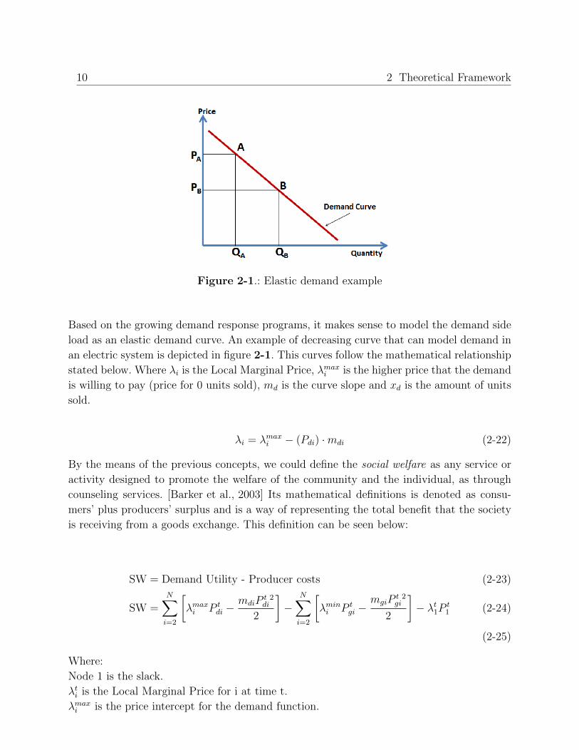
Figure 2-3.: MATLAB interior-point algorithm
Figure 2-3 depicts the fmincon path when solving a minimization for the MATLAB function
peaks(). This algorithm will be used to solve the non-linear power flow and find the market
equilibria that were proposed.
3. Market equilibrium in power systems
without network and storage
constraints
Since the main goal of this thesis is to find market equilibrium solutions (Monopoly and
Perfect Copetition) in power systems with network constraints, elastic demands and storage
devices, it is important to introduce a discussion about market equilibrium points without
storage and network considerations. In this chapter we define four equilibrium points (Mono-
poly, Nash-Cournot, Stackelberg and Perfect Competition). Section A.1 (Annex 1: Market
Equilibrium Solutions) presents an analytic approach developed by [DeOliveira, 2019] for
each of model assuming a simple two producer with an elastic demand without network and
storage constraints.
3.1. Monopolistic Solution
Monopoly markets appear when a single company controls the production of a specific good.
In the power market, this kind of behaviour can seriously harm the social welfare by ri-
sing the prices to maximize the producers welfare, specially in markets where there is not a
demand response program. According to [Xin and Sainan, 2010], monopolies show the follo-
wing characteristics in practice:
Non-openness of the data, market information block of transactions and real estate
transactions are carried out separately between developers and consumers.
The Location Market Structure of the real estate oligopoly, makes monopoly profits
exit in the real estate business, so the price of real estate transaction must exceed the
value.
There is a superiority of the seller bidding first in the real estate market, leading the
real estate transaction price is higher than its equilibrium price
A complete development for this equilibrium using an analytic approach can be found in
section A.1.3,

3.2 Nash-Cournot Equilibrium 15
3.2. Nash-Cournot Equilibrium
A Cournot model is defined in [Xiong et al., 2009] as a game model which is about making
decision of output. Nowadays, it is one of the classical models which research compete beha-
vior of manufacturers in the duopolies market. In recent years, the Cournot model has been
extended and has contained factors such as: incomplete information, dynamism and bounded
rationality.
This kind of games can be solver by finding their Nash equilibrium. This equilibrium is a
concept of game theory where the optimal outcome of a game is one where no player has an
incentive to deviate from his chosen strategy after considering an opponent’s choice. Given
the complex matter of this approach, in this document we will only find this equilibrium in
unconstrained models.
A complete development for this equilibrium using an analytic approach can be found in
section A.1.5,
3.3. Stackelberg Equilibrium
The Stackelberg Equilibrium is a game by game theory approach. [Policonomics, 2019] define
it as a sequential game (not simultaneous as in Cournot’s model) where there are two firms,
which sell homogeneous products, and are subject to the same demand and cost functions.
One firm, the leader, is perhaps better known or has greater brand equity, and is, therefore,
better placed to decide first which quantity to sell, and the other firm, the follower, observes
this and decides on its production quantity
In [Lin et al., 2018] a complete analysis in oligopoly competition is found using Stackelberg
theory. They explore the competitive mechanism of firms in a duopolistic market and cons-
tructs a model of duopolistic firms optimal output and maximum profit according to the
Stackelberg Leadership Model. Given the complex matter of this approach, in this document
we will only find this equilibrium in unconstrained models.
A complete development for this equilibrium using an analytic approach can be found in
section A.1.6,
3.4. Perfect Competition
This type of equilibrium is the simplest and the most widely studied, as said in the paper of
[Wang et al., 2018], the most important conditions for a perfect market to appear is that all

16 3 Market equilibrium in power systems without network and storage constraints
firms are price takers and every player has perfect information. Given that conditions and
by the requirement that all firms have a relatively small market share, it is not possible to
see a perfect competition in the real power market. Anyway, since this solution bring the
highest of the social welfare among the equilibria, it can be used as a reference to calculate
the deadweight loss of an imperfect market.
Figure 3-1.: Example of perfect competition in a market
Finally, figure 3-1 shows the point of perfect competition in a supply vs demand graph.
A complete development for this equilibrium using an analytic approach can be found in
section A.1.2.
3.5. Comparison analysis
In section A.1 (Annex 1: Market Equilibrium Solutions), an numerical example is provided
for the above-defined equilibrium models. It is assumed a simple 1-hour market with two
producers with an elastic demand without network and storage constraints. Figure 3-2 shows
the results.

3.5 Comparison analysis 17
0 10 20 30 40 50x1 + x2
0
10
20
30
40
50
60
[$/M
Wh]
(19.7,
30.3)
(26.0,
24.0)
(27.5,
22.5)
(28.8,
21.2)
(29.0,
21.0)
(38.7,
11.3)
MonopolyNash-CournotRegulatoryStackelberg (L2)Stackelberg (L1)Perfect Competition
Equilibrium Solutions (Demand Curves)
Figure 3-2.: Equilibrium solutions for a simple example
From Figure 3-2 and Table A-2 included in the appendix, we can observe that perfect
competition operating point corresponds to the best solution from social welfare viewpoint.
Monopolistic solution is the best from producer viewpoint but a significant welfare loss since
the demand is depressed and marginal prices the highest. Oligopolistic solutions are inter-
mediate.
In the next chapter, we extend the analysis for constrained systems considering the extreme
solutions depicted in Fig. 3-2: Perfect competition and monopolistic solution. Oligopolistic
solutions such as Nash and Stackelberg for constrained systems are out of scope of this work
and matter of future research.

4. Market equilibrium in power systems
with network and storage constraints
4.1. Network Model and Constraints
The formulation stated at 2.3 will be implemented in MATLAB in order to create a network
model that can be solved using fmincon (explained in section 2.7). Additional to the network
constraints given by the Ybus matrix and the power flow equations, the following will be
included:
Simulation time: Number of hours to simulate, leaving this as a parameter may help
to generalize the study case in the future.
Minimum and maximum voltage: Security constraints of voltage that every node
in the system must fulfill. If the voltage in the nodes is too far away from the slack
node, the system could become unstable and suffer a voltage collapse.
Battery capacity: Maximum energy that the energy storage device can accumulate.
Battery maximum usage: Percentage of the total battery capacity that the aggre-
gator can use to buy and sell energy and make profit from it.
Minimum and maximum power: Physical limitations of the batteries ripple and
the wind production. A limit to the reactive power will also be set since the machines
can not operate outside an specific power factor.
Line limits: Since there are limits in the current that can flow through a grid line,
it is necessary to include constraints in the maximum power that can flow. Changing
those limits will allow us to include and analysis of the effect from line limits in the
congestion fee.
4.2. Optimal Power Flow Problem
Each of the equilibrium points that we will study requires a different OPF formulation. In
this section we will define the optimization problems assuming that the constraints denoted
as The AC Network Model are the ones written in section 2.3.
4.2 Optimal Power Flow Problem 19
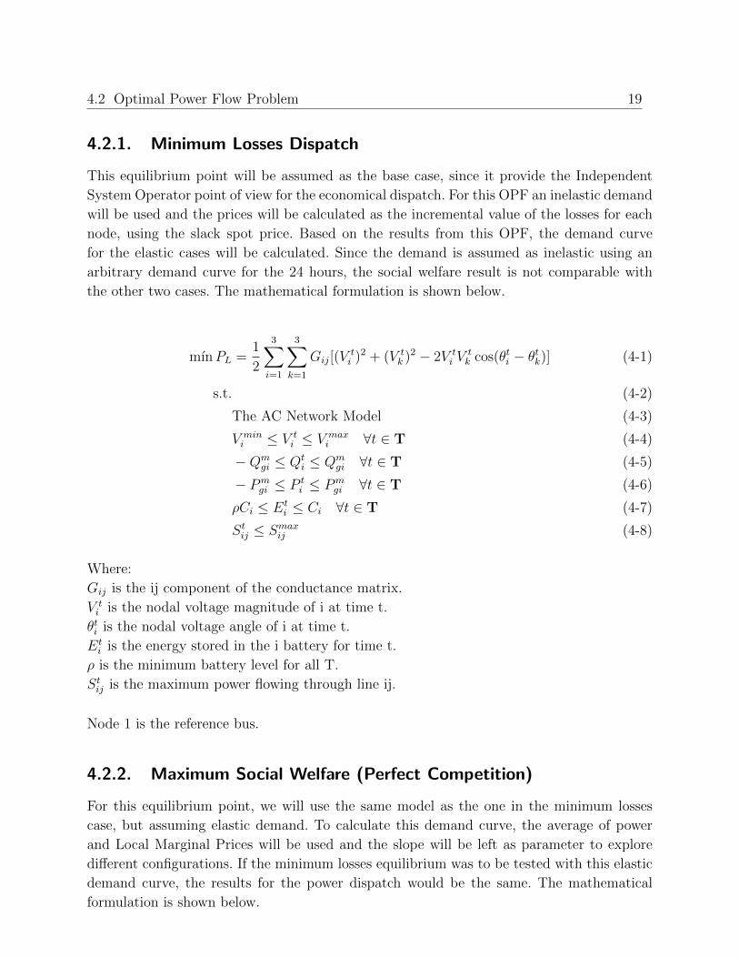
4.2.1. Minimum Losses Dispatch
This equilibrium point will be assumed as the base case, since it provide the Independent
System Operator point of view for the economical dispatch. For this OPF an inelastic demand
will be used and the prices will be calculated as the incremental value of the losses for each
node, using the slack spot price. Based on the results from this OPF, the demand curve
for the elastic cases will be calculated. Since the demand is assumed as inelastic using an
arbitrary demand curve for the 24 hours, the social welfare result is not comparable with
the other two cases. The mathematical formulation is shown below.
mınPL =1
2
3∑i=1
3∑k=1
Gij[(Vti )2 + (V t
k )2 − 2V ti V
tk cos(θti − θtk)] (4-1)
s.t. (4-2)
The AC Network Model (4-3)
V mini ≤ V t
i ≤ V maxi ∀t ∈ T (4-4)
−Qmgi ≤ Qt
i ≤ Qmgi ∀t ∈ T (4-5)
− Pmgi ≤ P t
i ≤ Pmgi ∀t ∈ T (4-6)
ρCi ≤ Eti ≤ Ci ∀t ∈ T (4-7)
Stij ≤ Smax
ij (4-8)
Where:
Gij is the ij component of the conductance matrix.
V ti is the nodal voltage magnitude of i at time t.
θti is the nodal voltage angle of i at time t.
Eti is the energy stored in the i battery for time t.
ρ is the minimum battery level for all T.
Stij is the maximum power flowing through line ij.
Node 1 is the reference bus.
4.2.2. Maximum Social Welfare (Perfect Competition)
For this equilibrium point, we will use the same model as the one in the minimum losses
case, but assuming elastic demand. To calculate this demand curve, the average of power
and Local Marginal Prices will be used and the slope will be left as parameter to explore
different configurations. If the minimum losses equilibrium was to be tested with this elastic
demand curve, the results for the power dispatch would be the same. The mathematical
formulation is shown below.

20 4 Market equilibrium in power systems with network and storage constraints
max Social Welfare = Demand Utility - Producer costs (4-9)
maxSW =N∑i=2
[λmaxi P t
di −mdiP
tdi2
2
]−
N∑i=2
[λmini P t
gi −mgiP
tgi2
2
]− λt1P t
1 (4-10)
s.t. The AC Network Model (4-11)
V mini ≤ V t
i ≤ V maxi ∀t ∈ T (4-12)
−Qmgi ≤ Qt
gi ≤ Qmgi ∀t ∈ T (4-13)
− Pmgi ≤ P t
gi ≤ Pmgi ∀t ∈ T (4-14)
ρCi ≤ Eti ≤ Ci ∀t ∈ T (4-15)
Stij ≤ Smax
ij (4-16)
λti = λmaxi −mdi · P t
di (4-17)
Where:
Gij is the ij component of the conductance matrix.
V ti is the nodal voltage magnitude of i at time t.
θti is the nodal voltage angle of i at time t.
Eti is the energy stored in the i battery for time t.
ρ is the minimum battery level for all T.
Stij is the maximum power flowing through line ij.
λti is the Local Marginal Price for i at time t.
λmaxi is the price intercept for the demand function.
mdi is the slope of the demand function.
Node 1 is the reference bus.
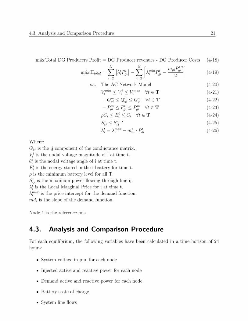
4.2.3. Monopoly Equilibrium
Finally, the monopoly equilibrium will be analyzed, the same model as the one in the maxi-
mum social welfare optimization will be used, but using a different objective function. This
function is modeled as the sum of the generator profits for all the nodes that are owned by
the monopoly company. In this equilibrium, the line flow constraints are even more impor-
tant since the company can use them to increase the Local Marginal Price by the means of
the congestion fee. The mathematical formulation is shown below.
4.3 Analysis and Comparison Procedure 21
max Total DG Producers Profit = DG Producer revenues - DG Producer Costs (4-18)
max Πtotal =N∑i=2
[λtiP
tgi
]−
N∑i=2
[λmini P t
gi −mgiP
tgi2
2
](4-19)
s.t. The AC Network Model (4-20)
V mini ≤ V t
i ≤ V maxi ∀t ∈ T (4-21)
−Qmgi ≤ Qt
gi ≤ Qmgi ∀t ∈ T (4-22)
− Pmgi ≤ P t
gi ≤ Pmgi ∀t ∈ T (4-23)
ρCi ≤ Eti ≤ Ci ∀t ∈ T (4-24)
Stij ≤ Smax
ij (4-25)
λti = λmaxi −mt
di · P tdi (4-26)
Where:
Gij is the ij component of the conductance matrix.
V ti is the nodal voltage magnitude of i at time t.
θti is the nodal voltage angle of i at time t.
Eti is the energy stored in the i battery for time t.
ρ is the minimum battery level for all T.
Stij is the maximum power flowing through line ij.
λti is the Local Marginal Price for i at time t.
λmaxi is the price intercept for the demand function.
mdi is the slope of the demand function.
Node 1 is the reference bus.
4.3. Analysis and Comparison Procedure
For each equilibrium, the following variables have been calculated in a time horizon of 24
hours:
System voltage in p.u. for each node
Injected active and reactive power for each node
Demand active and reactive power for each node
Battery state of charge
System line flows

22 4 Market equilibrium in power systems with network and storage constraints
System Local Marginal Prices
System hourly losses
In addition to this, the social welfare, total losses, total profit for each company, minimum,
maximum and mean Local Marginal Prices will be calculated for each scenario. Finally, some
variations in the system status, like disabling the energy storage device or including tight
line constraints will be studied.
5. Study case
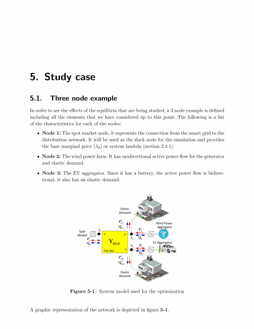
5.1. Three node example
In order to see the effects of the equilibria that are being studied, a 3 node example is defined
including all the elements that we have considered up to this point. The following is a list
of the characteristics for each of the nodes:
Node 1: The spot market node, it represents the connection from the smart grid to the
distribution network. It will be used as the slack node for the simulation and provides
the base marginal price (λ0) or system lambda (section 2.4.1).
Node 2: The wind power farm. It has unidirectional active power flow for the generator
and elastic demand.
Node 3: The EV aggregator. Since it has a battery, the active power flow is bidirec-
tional, it also has an elastic demand.
P1
3
2λ1
Q1
1
YBUS
λ2
λ3
P2
Q2
S
=
P3
Q3
S
=
PD3*
QD3*
SpotMarket
The Net
Wind PowerAggregator
EV Aggregator
ElasticDemand
ElasticDemand
PD3*2
QD3*2
Figure 5-1.: System model used for the optimization
A graphic representation of the network is depicted in figure 5-1.
24 5 Study case
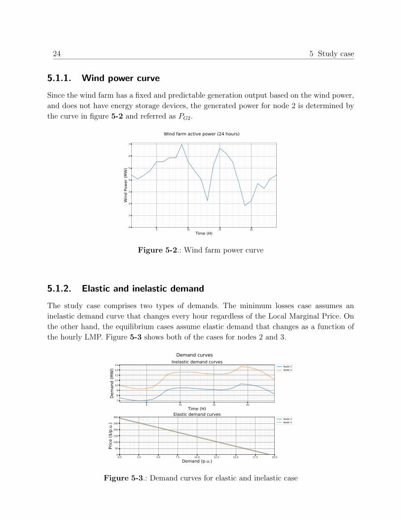
5.1.1. Wind power curve
Since the wind farm has a fixed and predictable generation output based on the wind power,
and does not have energy storage devices, the generated power for node 2 is determined by
the curve in figure 5-2 and referred as PG2.
5 10 15 20Time (H)
0
1
2
3
4
5
6
7
Win
d Po
wer (
MW
)
Wind farm active power (24 hours)
Figure 5-2.: Wind farm power curve
5.1.2. Elastic and inelastic demand
The study case comprises two types of demands. The minimum losses case assumes an
inelastic demand curve that changes every hour regardless of the Local Marginal Price. On
the other hand, the equilibrium cases assume elastic demand that changes as a function of
the hourly LMP. Figure 5-3 shows both of the cases for nodes 2 and 3.
5 10 15 20Time (H)
7
8
9
10
11
12
13
14
Dem
and
(MW
)
Inelastic demand curvesNode 2Node 3
0.0 2.5 5.0 7.5 10.0 12.5 15.0 17.5 20.0Demand (p.u.)
0
50
100
150
200
250
300
Price
($/p
.u.)
Elastic demand curvesNode 2Node 3
Demand curves
Figure 5-3.: Demand curves for elastic and inelastic case
5.1 Three node example 25
Demand curves in figure 5-3 are referred from now on as PD2, PD3 and λ2, λ3
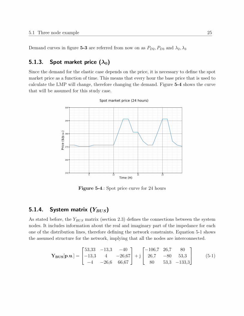
5.1.3. Spot market price (λ0)
Since the demand for the elastic case depends on the price, it is necessary to define the spot
market price as a function of time. This means that every hour the base price that is used to
calculate the LMP will change, therefore changing the demand. Figure 5-4 shows the curve
that will be assumed for this study case.
5 10 15 20Time (H)
250
260
270
280
290
300
Price
($/p
.u.)
Spot market price (24 hours)
Figure 5-4.: Spot price curve for 24 hours
5.1.4. System matrix (YBUS)
As stated before, the YBUS matrix (section 2.3) defines the connections between the system
nodes. It includes information about the real and imaginary part of the impedance for each
one of the distribution lines, therefore defining the network constraints. Equation 5-1 shows
the assumed structure for the network, implying that all the nodes are interconnected.
YBUS[p.u.] =
53,33 −13,3 −40
−13,3 4 −26,67
−4 −26,6 66,67
+ j
−106,7 26,7 80
26,7 −80 53,3
80 53,3 −133,3
(5-1)
26 5 Study case
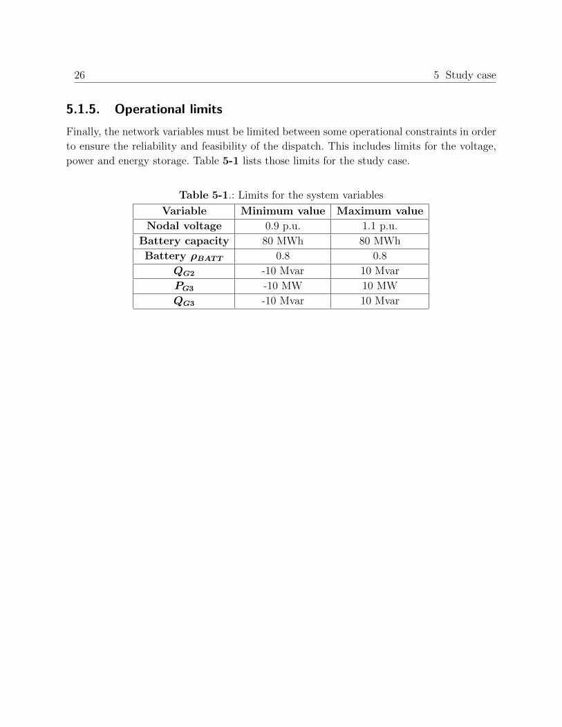
5.1.5. Operational limits
Finally, the network variables must be limited between some operational constraints in order
to ensure the reliability and feasibility of the dispatch. This includes limits for the voltage,
power and energy storage. Table 5-1 lists those limits for the study case.
Table 5-1.: Limits for the system variables
Variable Minimum value Maximum value
Nodal voltage 0.9 p.u. 1.1 p.u.
Battery capacity 80 MWh 80 MWh
Battery ρBATT 0.8 0.8
QG2 -10 Mvar 10 Mvar
PG3 -10 MW 10 MW
QG3 -10 Mvar 10 Mvar
6. Results
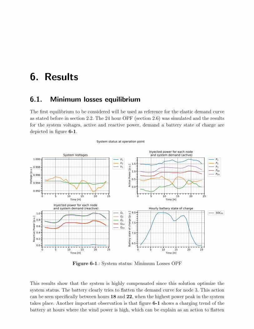
6.1. Minimum losses equilibrium
The first equilibrium to be considered will be used as reference for the elastic demand curve
as stated before in section 2.2. The 24 hour OPF (section 2.6) was simulated and the results
for the system voltages, active and reactive power, demand a battery state of charge are
depicted in figure 6-1.
0 5 10 15 20 25Time [H]
0.992
0.994
0.996
0.998
1.000
Volta
ge [p
.u.]
System VoltagesV1V2V3
0 5 10 15 20 25Time [H]
0.0
0.5
1.0
1.5
Activ
e Po
wer [
p.u.
]
Inyected power for each node and system demand (active)
P1P2P3PD2PD3
0 5 10 15 20 25Time [H]
0.0
0.2
0.4
0.6
0.8
1.0
Reac
tive
Powe
r [p.
u.]
Inyected power for each node and system demand (reactive)
Q1Q2Q3QD2QD3
0 5 10 15 20 25Time [H]
6.5
7.0
7.5
8.0
Batte
ry st
ate
of c
harg
e [p
.u.]
Hourly battery state of chargeSOCP3
System status at operation point
Figure 6-1.: System status: Minimum Losses OPF
This results show that the system is highly compensated since this solution optimize the
system status. The battery clearly tries to flatten the demand curve for node 3. This action
can be seen specifically between hours 18 and 22, when the highest power peak in the system
takes place. Another important observation is that figure 6-1 shows a charging trend of the
battery at hours where the wind power is high, which can be explain as an action to flatten

28 6 Results
the net power curve. It can also be seen that the reactive power for each node is compensated
with local generation except when the local generation can not supply the local demand.
0 5 10 15 20 25Time [H]
0.0
0.2
0.4
0.6
0.8
1.0
1.2
Line
Flow
[p.u
.]
S12S13S23
System line flows
Figure 6-2.: System Line Flows: Minimum
Losses
0 5 10 15 20 25Time [H]
270
275
280
285
290
295
Price
[$/p
.u.]
System Prices0
2
3
0 5 10 15 20 25Time [H]
0.008
0.009
0.010
0.011
0.012
0.013
Price
[p.u
.]
System LossesLosses
System prices and losses
Figure 6-3.: Nodal Prices and System Los-
ses: Minimum Losses
To completely determine the system status, we also calculated the system line flows that
are shown in figure 6-2. High line flow in the S13 branch may suggest that the slack power
is mainly used to charge the battery. Nodal prices and system losses are important as well,
since they are key to study the market equilibrium and compare it with the others, they are
shown in figure 6-3. Both Local Marginal Prices and system losses show a clear correlation
with the peak hours and between themselves, since the losses are used as a basis to calculate
the incremental factor which determines the price in the inelastic approach.

6.2 Perfect competition 29
6.2. Perfect competition
0 5 10 15 20 25Time [H]
0.992
0.994
0.996
0.998
1.000
1.002
1.004
Volta
ge [p
.u.]
System VoltagesV1V2V3
0 5 10 15 20 25Time [H]
1.0
0.5
0.0
0.5
1.0
1.5
2.0
2.5
Activ
e Po
wer [
p.u.
]
Inyected power for each node and system demand (active)
P1P2P3PD2PD3
0 5 10 15 20 25Time [H]
0.0
0.2
0.4
0.6
0.8
Reac
tive
Powe
r [p.
u.]
Inyected power for each node and system demand (reactive)
Q1Q2Q3QD2QD3
0 5 10 15 20 25Time [H]
6.50
6.75
7.00
7.25
7.50
7.75
8.00
Batte
ry st
ate
of c
harg
e [p
.u.]
Hourly battery state of chargeSOCP3
System status at operation point
Figure 6-4.: System status: Maximum SW
Perfect competition is the second system status that we are studying, it follows the same
principle as the minimum losses approach, but uses an economical approach based on the
maximization of the social welfare. The power flow that was executed is depicted in figure
6-4. Since the state variables of the system are now related with the social welfare, all of
them show a direct correlation with the slack price. Same as before, that battery tries to
flatten the net power curve which is directly related with the Local Marginal Price in the
elastic approach. Between hours 12 - 13, and 20 - 21 a clear increase in the prices happen,
which trigger the battery discharge.
Finally, the same calculations that the ones for the previous equilibrium are shown in figures
6-5 and 6-6. Since the prices and demands are now directly related through the elastic
demand formulation, it is clear that figures 6-6 and 6-4 are tightly correlated. We can see
that the system losses are also very low, which is consistent with the theoretical formulation,
which states that the maximum social welfare and the minimum losses optimizations are
equivalent.

30 6 Results
0 5 10 15 20 25Time [H]
0.00
0.25
0.50
0.75
1.00
1.25
1.50
1.75
Line
Flow
[p.u
.]
S12S13S23
System line flows
Figure 6-5.: System Line Flows: Maximum
SW
0 5 10 15 20 25Time [H]
270
275
280
285
290
Price
[$/p
.u.]
System Prices0
2
3
0 5 10 15 20 25Time [H]
0.005
0.010
0.015
0.020
Price
[p.u
.]
System LossesLosses
System prices and losses
Figure 6-6.: Nodal Prices and System Los-
ses: Maximum SW
6.3. Monopoly scenario
0 5 10 15 20 25Time [H]
0.90
0.92
0.94
0.96
0.98
1.00
Volta
ge [p
.u.]
System VoltagesV1V2V3
0 5 10 15 20 25Time [H]
2
0
2
4
6
8
10
Activ
e Po
wer [
p.u.
]
Inyected power for each node and system demand (active)
P1P2P3PD2PD3
0 5 10 15 20 25Time [H]
0
2
4
6
Reac
tive
Powe
r [p.
u.]
Inyected power for each node and system demand (reactive)
Q1Q2Q3QD2QD3
0 5 10 15 20 25Time [H]
6.50
6.75
7.00
7.25
7.50
7.75
8.00
Batte
ry st
ate
of c
harg
e [p
.u.]
Hourly battery state of chargeSOCP3
System status at operation point
Figure 6-7.: System status: Maximum π2 + π3
The final equilibrium to be studied is the monopoly scenario. Figure 6-7 shows a clearly
erratic behaviour of the system state variables, the nodal voltages are reaching the lower
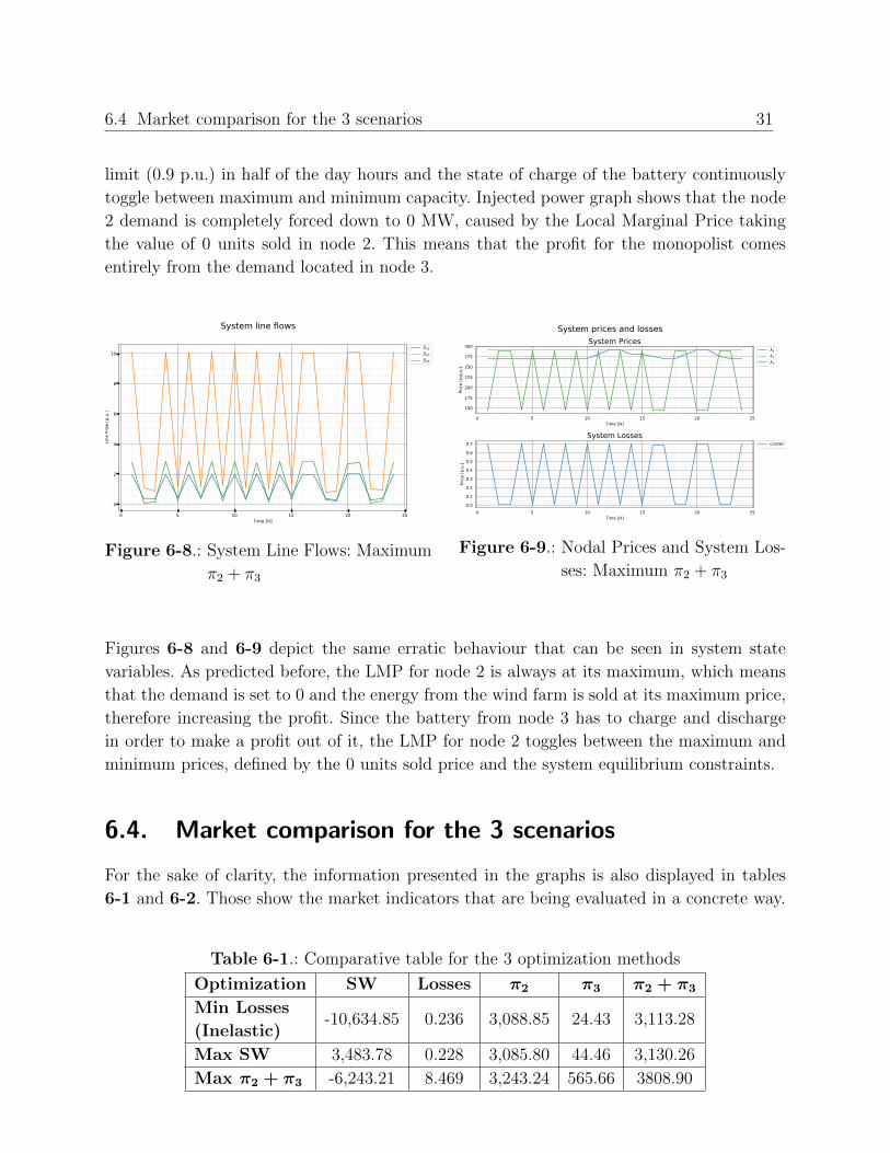
6.4 Market comparison for the 3 scenarios 31
limit (0.9 p.u.) in half of the day hours and the state of charge of the battery continuously
toggle between maximum and minimum capacity. Injected power graph shows that the node
2 demand is completely forced down to 0 MW, caused by the Local Marginal Price taking
the value of 0 units sold in node 2. This means that the profit for the monopolist comes
entirely from the demand located in node 3.
0 5 10 15 20 25Time [H]
0
2
4
6
8
10
Line
Flow
[p.u
.]
S12S13S23
System line flows
Figure 6-8.: System Line Flows: Maximum
π2 + π3
0 5 10 15 20 25Time [H]
150
175
200
225
250
275
300
Price
[$/p
.u.]
System Prices0
2
3
0 5 10 15 20 25Time [H]
0.00.10.20.30.40.50.60.7
Price
[p.u
.]
System LossesLosses
System prices and losses
Figure 6-9.: Nodal Prices and System Los-
ses: Maximum π2 + π3
Figures 6-8 and 6-9 depict the same erratic behaviour that can be seen in system state
variables. As predicted before, the LMP for node 2 is always at its maximum, which means
that the demand is set to 0 and the energy from the wind farm is sold at its maximum price,
therefore increasing the profit. Since the battery from node 3 has to charge and discharge
in order to make a profit out of it, the LMP for node 2 toggles between the maximum and
minimum prices, defined by the 0 units sold price and the system equilibrium constraints.
6.4. Market comparison for the 3 scenarios
For the sake of clarity, the information presented in the graphs is also displayed in tables
6-1 and 6-2. Those show the market indicators that are being evaluated in a concrete way.
Table 6-1.: Comparative table for the 3 optimization methods
Optimization SW Losses π2 π3 π2 + π3
Min Losses
(Inelastic)-10,634.85 0.236 3,088.85 24.43 3,113.28
Max SW 3,483.78 0.228 3,085.80 44.46 3,130.26
Max π2 + π3 -6,243.21 8.469 3,243.24 565.66 3808.90
32 6 Results
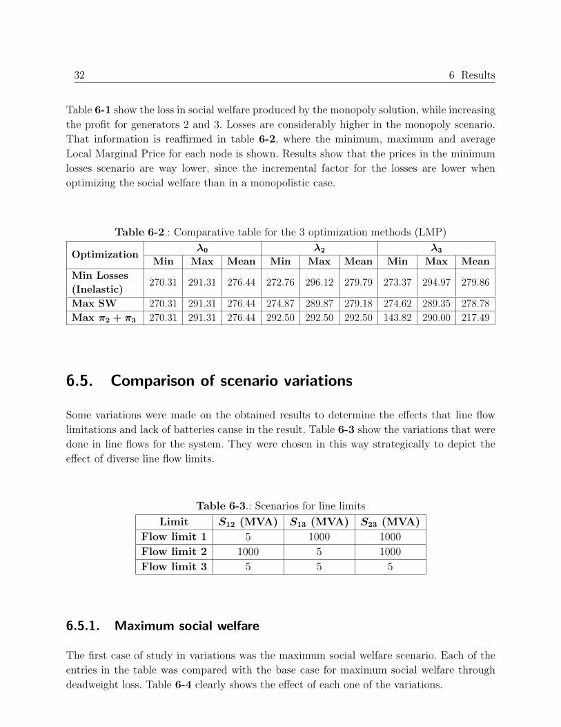
Table 6-1 show the loss in social welfare produced by the monopoly solution, while increasing
the profit for generators 2 and 3. Losses are considerably higher in the monopoly scenario.
That information is reaffirmed in table 6-2, where the minimum, maximum and average
Local Marginal Price for each node is shown. Results show that the prices in the minimum
losses scenario are way lower, since the incremental factor for the losses are lower when
optimizing the social welfare than in a monopolistic case.
Table 6-2.: Comparative table for the 3 optimization methods (LMP)
Optimizationλ0 λ2 λ3
Min Max Mean Min Max Mean Min Max Mean
Min Losses
(Inelastic)270.31 291.31 276.44 272.76 296.12 279.79 273.37 294.97 279.86
Max SW 270.31 291.31 276.44 274.87 289.87 279.18 274.62 289.35 278.78
Max π2 + π3 270.31 291.31 276.44 292.50 292.50 292.50 143.82 290.00 217.49
6.5. Comparison of scenario variations
Some variations were made on the obtained results to determine the effects that line flow
limitations and lack of batteries cause in the result. Table 6-3 show the variations that were
done in line flows for the system. They were chosen in this way strategically to depict the
effect of diverse line flow limits.
Table 6-3.: Scenarios for line limits
Limit S12 (MVA) S13 (MVA) S23 (MVA)
Flow limit 1 5 1000 1000
Flow limit 2 1000 5 1000
Flow limit 3 5 5 5
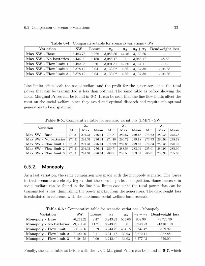
6.5.1. Maximum social welfare
The first case of study in variations was the maximum social welfare scenario. Each of the
entries in the table was compared with the base case for maximum social welfare through
deadweight loss. Table 6-4 clearly shows the effect of each one of the variations.
6.5 Comparison of scenario variations 33
Table 6-4.: Comparative table for scenario variations - SW
Variation SW Losses π2 π3 π2 + π3 Deadweight loss
Max SW - Base 3,483.78 0.228 3,085.80 44.46 3,130.26 -
Max SW - No batteries 3,434.90 0.180 3,085.17 0.0 3,085.17 -48.88
Max SW - Flow limit 1 3,482.36 0.20 3,091.31 42.80 3,134.11 -1.42
Max SW - Flow limit 2 3,378.12 0.04 3,133.02 4.36 3,137.38 -105.68
Max SW - Flow limit 3 3,378.12 0.04 3,133.02 4.36 3,137.38 -105.66
Line limits affect both the social welfare and the profit for the generators since the total
power that can be transmitted is less than optimal. The same table as before showing the
Local Marginal Prices can be found in 6-5. It can be seen that the line flow limits affect the
most on the social welfare, since they avoid and optimal dispatch and require sub-optimal
generators to be dispatched.
Table 6-5.: Comparative table for scenario variations (LMP) - SW
Variationλ0 λ2 λ3
Min Max Mean Min Max Mean Min Max Mean
Max SW - Base 270.31 291.31 276.44 274.87 289.87 279.18 274.62 289.35 278.78
Max SW - No batteries 270.31 291.31 276.44 274.40 290.77 279.18 273.73 290.98 278.78
Max SW - Flow limit 1 270.31 291.31 276.44 274.99 289.86 279.67 274.83 289.35 278.95
Max SW - Flow limit 2 270.31 291.31 276.44 280.71 288.53 283.01 285.01 286.96 285.60
Max SW - Flow limit 3 270.31 291.31 276.44 280.71 288.53 283.01 285.01 286.96 285.60
6.5.2. Monopoly
As a last variation, the same comparison was made with the monopoly scenario. The losses
in that scenario are clearly higher that the ones in perfect competition. Some increase in
social welfare can be found in the line flow limits case since the total power that can be
transmitted is less, diminishing the power market from the generators. The deadweight loss
is calculated in reference with the maximum social welfare base scenario.
Table 6-6.: Comparative table for scenario variations - Monopoly
Variation SW Losses π2 π3 π2 + π3 Deadweight loss
Monopoly - Base -6,243.21 8.47 3,243.24 565.66 808.90 -9,726.99
Monopoly - No batteries -9,531.41 11.21 3,243.23 0.0 3,243.23 -13,015.19
Monopoly - Flow limit 1 2,613.86 0.79 3,243.23 494.18 3,737.42 -869.92
Monopoly - Flow limit 2 3,120.90 0.11 3,241.18 30.93 3,272.11 -362.88
Monopoly - Flow limit 3 3,104.78 0.09 3,242.40 34.63 3,277.03 -379.00
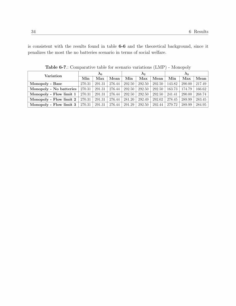
Finally, the same table as before with the Local Marginal Prices can be found in 6-7, which
34 6 Results
is consistent with the results found in table 6-6 and the theoretical background, since it
penalizes the most the no batteries scenario in terms of social welfare.
Table 6-7.: Comparative table for scenario variations (LMP) - Monopoly
Variationλ0 λ2 λ3
Min Max Mean Min Max Mean Min Max Mean
Monopoly - Base 270.31 291.31 276.44 292.50 292.50 292.50 143.82 290.00 217.49
Monopoly - No batteries 270.31 291.31 276.44 292.50 292.50 292.50 163.73 174.79 166.62
Monopoly - Flow limit 1 270.31 291.31 276.44 292.50 292.50 292.50 241.41 290.00 268.74
Monopoly - Flow limit 2 270.31 291.31 276.44 281.20 292.49 292.02 278.45 289.99 283.45
Monopoly - Flow limit 3 270.31 291.31 276.44 291.29 292.50 292.44 279.72 289.99 284.95

7. Conclusions and recommendations
7.1. Conclusions
The main goal of analyzing and comparing the proposed market equilibria was achieved. A
simulation and optimization tool was build using MATLAB and its toolbox and the results
were validated by analyzing several variations of the base scenario.
The base optimization for the minimum losses scenario found a system set-point that settled
the nodal voltage close to 1 p.u. and fed the demand of each node by using the local gene-
ration, looking forward to lower the flow through the system lines. This kind of actions also
flattened the net demand of the nodes, which is a typical behaviour of the losses minimiza-
tion problem. Since this case demand was assumed as inelastic, it was also a helpful tool to
estimate the elastic demand curve. An important observation about the battery behaviour
is that it was usually charging during the peak hours of the wind generation, but started to
discharge when the wind was at its lower point.
The maximum social welfare scenario showed a similar behaviour in terms of the battery
state of charge, but it was noticeable that both the power dispatch and the demand load
were directly related with the spot market price. In terms of total losses, this dispatch should
be exactly the same as the minimum losses dispatch if the system were exactly the same.
Finally, the monopoly scenario is an example of the damage that enough market power could
do to a system. The voltages show a clear disruption from the nominal voltage, and the ac-
tive and reactive power behaviour is highly erratic. The state of charge of the battery shows
that it is completing as much battery cycles as possible, increasing the total profit for gene-
rator 3. This kind of behaviour together with abrupt changes in the Local Marginal Prices
increases the total profit for the aggregator but could significantly lower the lifespan of the
battery depending on the technology. Figure 6-9 also shows that the total system losses are
considerably higher than in the social welfare scenario, same as the line flows through the
system, which is an explanation for the increase in losses.
As for the Local Marginal Prices, table 6-2 shows that the mean price for both nodes 2 and
3 is higher than the ones in the maximum social welfare scenario, but the minimum price for
the battery node is considerably lower, this is explained by the fact that the EV aggregator

36 7 Conclusions and recommendations
prefers to charge the batteries at the lowest price possible and discharge them at the highest.
7.2. Recommendations and future work
Future implementations for this work should include a complete constrained model for the
Nash-Cournot and Stackelberg equilibria. To accomplish that level of completeness, it may
be necessary to include heuristic optimization to solve the bi-level problem that appears,
some approaches like Ant Colony Optimization can be found in [Tapia, 2017].
Another improvement that could be made to this approach is to decouple the optimization
problem from the power flow. This would increase the computational effort required but will
also enable to write more complex optimization problems easily.
Bibliography
[Abdi et al., 2017] Abdi, H., Mohammadi-ivatloo, B., Javadi, S., Khodaei, A. R., and Deh-
navi, E. (2017). Chapter 7 - energy storage systems. In Gharehpetian, G. and Agah, S.
M. M., editors, Distributed Generation Systems, pages 333 – 368. Butterworth-Heinemann.
[Artakusuma et al., 2014] Artakusuma, D. D., Afrisal, H., Cahyadi, A. I., and Wahyung-
goro, O. (2014). Battery management system via bus network for multi battery electric
vehicle. In 2014 International Conference on Electrical Engineering and Computer Science
(ICEECS), pages 179–181.
[Barai et al., 2015] Barai, G. R., Krishnan, S., and Venkatesh, B. (2015). Smart metering
and functionalities of smart meters in smart grid - a review. In 2015 IEEE Electrical
Power and Energy Conference (EPEC), pages 138–145.
[Barker et al., 2003] Barker, R. L. et al. (2003). The social work dictionary.
[Delgadillo et al., 2010] Delgadillo, A., Duenas, P., Reneses, J., and Barquın, J. (2010).
Analysis of an electricity market equilibrium model with large-scale penetration of wind
energy. In 2010 7th International Conference on the European Energy Market, pages 1–6.
[DeOliveira, 2019] DeOliveira, P. (2019). Notes for course iele4109 - los andes university.
[Glavitsch, 1991] Glavitsch, H. (1991). Optimal power flow algorithms.
[He et al., 2015] He, Y., Sharma, R., and Bozchalui, M. C. (2015). Optimal battery pricing
under uncertain demand management. In 2015 IEEE Power Energy Society Innovative
Smart Grid Technologies Conference (ISGT), pages 1–6.
[Herig, 2003] Herig, C. (2003). Photovoltaics as a distributed resource - making the va-
lue connection. In 2003 IEEE Power Engineering Society General Meeting (IEEE Cat.
No.03CH37491), volume 3, pages 1334–1338 Vol. 3.
[Heydt et al., 2012] Heydt, G. T., Chowdhury, B. H., Crow, M. L., Haughton, D., Kiefer,
B. D., Meng, F., and Sathyanarayana, B. R. (2012). Pricing and control in the next
generation power distribution system. IEEE Transactions on Smart Grid, 3(2):907–914.
[Huang et al., 2012] Huang, B. B., Xie, G. H., Kong, W. Z., and Li, Q. H. (2012). Study
on smart grid and key technology system to promote the development of distributed
generation. In IEEE PES Innovative Smart Grid Technologies, pages 1–4.
38 Bibliography
[Lin et al., 2018] Lin, T. T., Hsu, S., and Chang, C. (2018). Analysis of stackelberg lea-
dership model output behavior under the mechanism of expanding market price. In 2018
IEEE International Conference on Industrial Engineering and Engineering Management
(IEEM), pages 1603–1607.
[MathWorks, 2019] MathWorks (2019). Optimization toolbox.
[Mutale et al., 2000] Mutale, J., Strbac, G., Curcic, S., and Jenkins, N. (2000). Allocation
of losses in distribution systems with embedded generation. IEE Proceedings-Generation,
Transmission and Distribution, 147(1):7–14.
[Negash and Kirschen, 2014] Negash, A. I. and Kirschen, D. S. (2014). Optimally designed
retail rates to incentivize demand response. In 2014 IEEE Conference on Technologies for
Sustainability (SusTech), pages 45–50.
[PJM, 2017] PJM (2017). Locational marginal pricing components.
[Policonomics, 2019] Policonomics (2019). Stackelberg game.
[Qinwei Duan, 2016] Qinwei Duan (2016). A price-based demand response scheduling model
in day-ahead electricity market. In 2016 IEEE Power and Energy Society General Meeting
(PESGM), pages 1–5.
[Root et al., 2017] Root, C., Presume, H., Proudfoot, D., Willis, L., and Masiello, R. (2017).
Using battery energy storage to reduce renewable resource curtailment. In 2017 IEEE
Power Energy Society Innovative Smart Grid Technologies Conference (ISGT), pages 1–
5.
[Tapia, 2017] Tapia, H. (2017). Optimal power flow application for active distribution net-
works using ant colony system algorithm. Master’s thesis, Universidad de Los Andes.
[Toquica, 2019] Toquica (2019). Mitigation of the impacts electric vehicles into electricity
markets - a bilevel optimization approach.
[Toro, 2018] Toro, C. (2018). Flujo de potencia Optimo multiobjetivo en un marco de ge-
neracion distribuida.
[Vani et al., 2012] Vani, S., Kopperundevi, R., Thilagavathi, T., Presath, R. K. A., and Ra-
jathy, R. (2012). Opf-based market clearing procedure using bacterial foraging algorithm
and auction-based market clearing procedures in a pool based electricity market — a
comparison. In 2012 IEEE Students’ Conference on Electrical, Electronics and Computer
Science, pages 1–5.
Bibliography 39
[Wafaa et al., 2016] Wafaa, M. B., Dessaint, L., and Kamwa, I. (2016). A market-based
approach of opf with consideration of voltage stability improvement. In 2016 IEEE Power
and Energy Society General Meeting (PESGM), pages 1–5.
[Wang et al., 2018] Wang, H., Deng, J., Wang, C., Sun, W., and Xie, N. (2018). Comparing
competition equilibrium with nash equilibrium in electric power market. CSEE Journal
of Power and Energy Systems, 4(3):299–304.
[Xin and Sainan, 2010] Xin, M. and Sainan, L. (2010). A study on the monopoly power of
china’s real estate market. In 2010 3rd International Conference on Information Mana-
gement, Innovation Management and Industrial Engineering, volume 4, pages 238–241.
[Xiong et al., 2009] Xiong, G., Li, L., and Liu, Y. (2009). The cournot model with incomplete
information based on the rdeu theory. In 2009 International Conference on Information
Management, Innovation Management and Industrial Engineering, volume 3, pages 471–
474.
[Zhao et al., 2014] Zhao, B., Shi, Y., and Dong, X. (2014). Pricing and revenue maximization
for battery charging services in phev markets. IEEE Transactions on Vehicular Technology,
63(4):1987–1993.
[Zhu, 2015] Zhu, J. (2015). Optimization of Power System Operation.
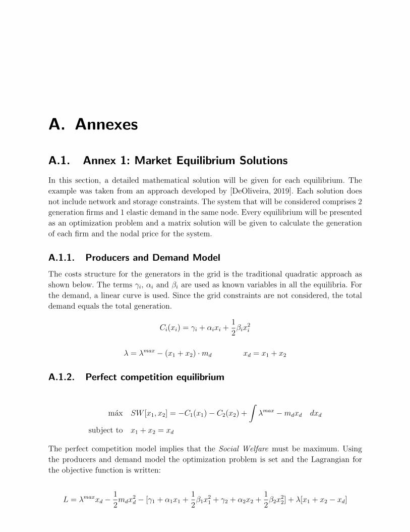
A. Annexes
A.1. Annex 1: Market Equilibrium Solutions
In this section, a detailed mathematical solution will be given for each equilibrium. The
example was taken from an approach developed by [DeOliveira, 2019]. Each solution does
not include network and storage constraints. The system that will be considered comprises 2
generation firms and 1 elastic demand in the same node. Every equilibrium will be presented
as an optimization problem and a matrix solution will be given to calculate the generation
of each firm and the nodal price for the system.
A.1.1. Producers and Demand Model
The costs structure for the generators in the grid is the traditional quadratic approach as
shown below. The terms γi, αi and βi are used as known variables in all the equilibria. For
the demand, a linear curve is used. Since the grid constraints are not considered, the total
demand equals the total generation.
Ci(xi) = γi + αixi +1
2βix
2i
λ = λmax − (x1 + x2) ·md xd = x1 + x2
A.1.2. Perfect competition equilibrium
max SW [x1, x2] = −C1(x1)− C2(x2) +
∫λmax −mdxd dxd
subject to x1 + x2 = xd
The perfect competition model implies that the Social Welfare must be maximum. Using
the producers and demand model the optimization problem is set and the Lagrangian for
the objective function is written:
L = λmaxxd −1
2mdx
2d − [γ1 + α1x1 +
1
2β1x
21 + γ2 + α2x2 +
1
2β2x
22] + λ[x1 + x2 − xd]

A.1 Annex 1: Market Equilibrium Solutions 41
Following the Lagrange method to solve non-linear optimization problems, the partial deri-
vatives are calculated and equal to 0.
∂L
∂x1= λ− α1 − β1x1 = 0
∂L
∂x2= λ− α2 − β2x2 = 0
∂L
∂xd= λ− λmax +mdxd = 0
∂L
∂λ= xd − x1 − x2 = 0
Finally, these equations are written as a matrix system to find a direct solution for the
producers and demand set-points.
xpc1xpc2xpcdλpc
=
−β1 0 0 1
0 −β2 0 1
0 0 md 1
1 1 −1 0
−1
α1
α2
λmax
0
A.1.3. Monopoly equilibrium
max Π[x1, x2] = λx1 − C1(x1) + λx2 − C2(x2)
where λ = λmax − (x1 + x2) ·md
For this equilibrium, the addition of the producers profit must be at its maximum. Since
the problem is unconstrained, a direct solution can be found by applying the first order
conditions.
∂Π
∂x1= λmax − 2mdx1 −mdx2 −mdx2 − α1 − β1x1 = 0
∂Π
∂x2= λmax − 2mdx2 −mdx1 −mdx1 − α2 − β2x2 = 0
Finally, the matrix representation is presented to find the direct solution for the equilibrium.
[xm1xm2
]=
[2md + β1 2md
2md 2md + β2
]−1 [λmax − α1
λmax − α2
]
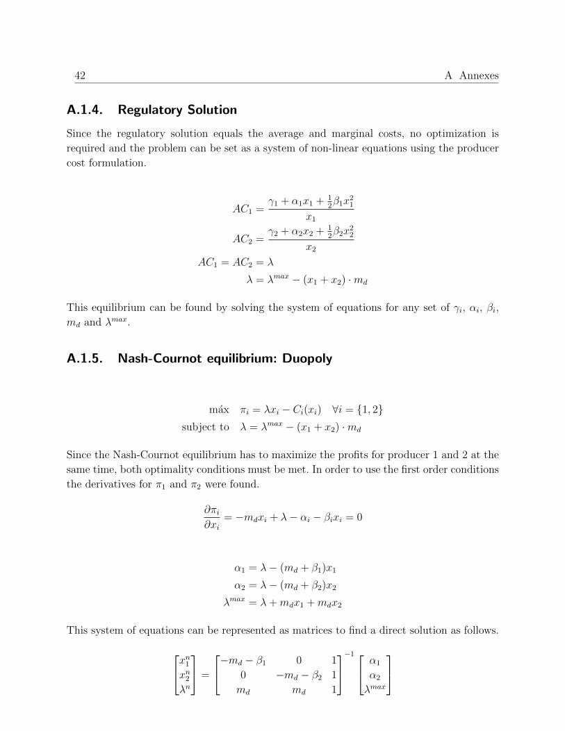
42 A Annexes
A.1.4. Regulatory Solution
Since the regulatory solution equals the average and marginal costs, no optimization is
required and the problem can be set as a system of non-linear equations using the producer
cost formulation.
AC1 =γ1 + α1x1 + 1
2β1x
21
x1
AC2 =γ2 + α2x2 + 1
2β2x
22
x2
AC1 = AC2 = λ
λ = λmax − (x1 + x2) ·md
This equilibrium can be found by solving the system of equations for any set of γi, αi, βi,
md and λmax.
A.1.5. Nash-Cournot equilibrium: Duopoly
max πi = λxi − Ci(xi) ∀i = {1, 2}subject to λ = λmax − (x1 + x2) ·md
Since the Nash-Cournot equilibrium has to maximize the profits for producer 1 and 2 at the
same time, both optimality conditions must be met. In order to use the first order conditions
the derivatives for π1 and π2 were found.
∂πi∂xi
= −mdxi + λ− αi − βixi = 0
α1 = λ− (md + β1)x1
α2 = λ− (md + β2)x2
λmax = λ+mdx1 +mdx2
This system of equations can be represented as matrices to find a direct solution as follows.
xn1xn2λn
=
−md − β1 0 1
0 −md − β2 1
md md 1
−1 α1
α2
λmax

A.1 Annex 1: Market Equilibrium Solutions 43
A.1.6. Stackelberg equilibrium
In the Stackelberg formulation, the leader solution must be in the follower’s solution set,
therefore, the problem is presented as a bi-level optimization with producer 2 as the leader
and producer 1 as the follower.
max π2 = x2 · [λmax −md(x1 + x2)]− C2(x2)
subject to x1 ≡ argmax π1 = x1 · [λmax −md(x1 + x2)]− C1(x1)
In order to solve the bi-level optimization using algebraic methods, it’s necessary to find an
expression for the follower solution in terms of the leader decision variable.
∂π1∂x1
= λmax − 2mdx1 −mdx2 − α1 − β1x1 = 0
x1 = A+Bx2 =λmax − α1
2md + β1+
−md
2md + β1x2
After finding that expression, it can be used to solve the univariate leader problem as follows.
∂π2∂x2
= λmax −mdA− α2 − [β2 + 2md(B + 1)] · x2 = 0
Finally, a direct solution for the problem is derived from this formulation.
xst2 =λmax −mdA− α2
β2 + 2md(B + 1)
xst1 = A+Bxst2
λst = λmax −md · (xst1 + xst2 )
A.1.7. Equilibrium Example: 2 Producers with Elastic Demand
In this section, an example will be given to present a numeric comparison of the equilibria
solutions found above. The following values will be assumed for the producers and demand
functions:
Producer 1: γ1 = 0 α1 = 10 β1 = 0,05
Producer 2: γ2 = 0 α2 = 10 β2 = 0,1
Demand: md = 1 λmax = 50
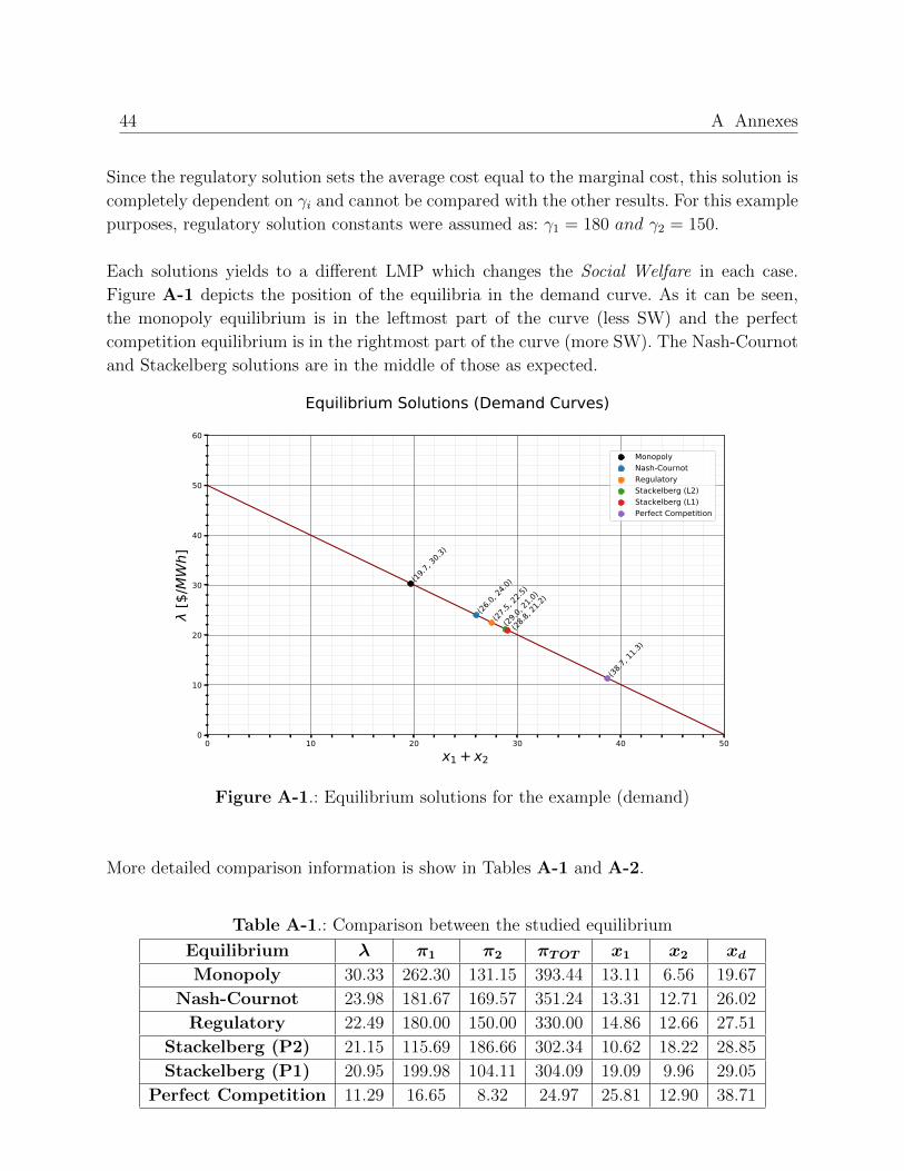
44 A Annexes
Since the regulatory solution sets the average cost equal to the marginal cost, this solution is
completely dependent on γi and cannot be compared with the other results. For this example
purposes, regulatory solution constants were assumed as: γ1 = 180 and γ2 = 150.
Each solutions yields to a different LMP which changes the Social Welfare in each case.
Figure A-1 depicts the position of the equilibria in the demand curve. As it can be seen,
the monopoly equilibrium is in the leftmost part of the curve (less SW) and the perfect
competition equilibrium is in the rightmost part of the curve (more SW). The Nash-Cournot
and Stackelberg solutions are in the middle of those as expected.
0 10 20 30 40 50x1 + x2
0
10
20
30
40
50
60
[$/M
Wh]
(19.7,
30.3)
(26.0,
24.0)
(27.5,
22.5)
(28.8,
21.2)
(29.0,
21.0)
(38.7,
11.3)
MonopolyNash-CournotRegulatoryStackelberg (L2)Stackelberg (L1)Perfect Competition
Equilibrium Solutions (Demand Curves)
Figure A-1.: Equilibrium solutions for the example (demand)
More detailed comparison information is show in Tables A-1 and A-2.
Table A-1.: Comparison between the studied equilibrium
Equilibrium λ π1 π2 πTOT x1 x2 xd
Monopoly 30.33 262.30 131.15 393.44 13.11 6.56 19.67
Nash-Cournot 23.98 181.67 169.57 351.24 13.31 12.71 26.02
Regulatory 22.49 180.00 150.00 330.00 14.86 12.66 27.51
Stackelberg (P2) 21.15 115.69 186.66 302.34 10.62 18.22 28.85
Stackelberg (P1) 20.95 199.98 104.11 304.09 19.09 9.96 29.05
Perfect Competition 11.29 16.65 8.32 24.97 25.81 12.90 38.71
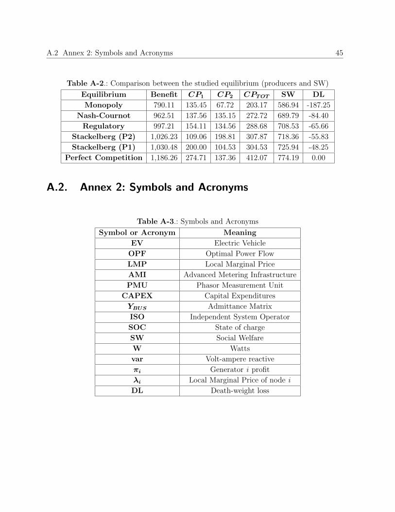
A.2 Annex 2: Symbols and Acronyms 45
Table A-2.: Comparison between the studied equilibrium (producers and SW)
Equilibrium Benefit CP1 CP2 CPTOT SW DL
Monopoly 790.11 135.45 67.72 203.17 586.94 -187.25
Nash-Cournot 962.51 137.56 135.15 272.72 689.79 -84.40
Regulatory 997.21 154.11 134.56 288.68 708.53 -65.66
Stackelberg (P2) 1,026.23 109.06 198.81 307.87 718.36 -55.83
Stackelberg (P1) 1,030.48 200.00 104.53 304.53 725.94 -48.25
Perfect Competition 1,186.26 274.71 137.36 412.07 774.19 0.00
A.2. Annex 2: Symbols and Acronyms
Table A-3.: Symbols and Acronyms
Symbol or Acronym Meaning
EV Electric Vehicle
OPF Optimal Power Flow
LMP Local Marginal Price
AMI Advanced Metering Infrastructure
PMU Phasor Measurement Unit
CAPEX Capital Expenditures
YBUS Admittance Matrix
ISO Independent System Operator
SOC State of charge
SW Social Welfare
W Watts
var Volt-ampere reactive
πi Generator i profit
λi Local Marginal Price of node i
DL Death-weight loss


![Proceedings of the ASME 2017 36th International Conference ......equilibrium equations are established considering both external ... body motion [6]. Given an offshore floating wind](https://img.pdfslide.net/doc/110x75/5e75b7c65e87be40774dcd84/proceedings-of-the-asme-2017-36th-international-conference-equilibrium-equations.jpg)


![Road Vehicle-Bridge Interaction considering Varied Vehicle ...downloads.hindawi.com/journals/sv/2018/1389628.pdf · the leand right wheel paths [].Here,an exponentially decreasing](https://img.pdfslide.net/doc/110x75/5e2fd82c0d07c92186326759/road-vehicle-bridge-interaction-considering-varied-vehicle-the-leand-right-wheel.jpg)