Market Valuation of Accrued Social Security Benefits

by

John Geanakoplos Yale University; and Santa Fe Institute

and

Stephen P. Zeldes

Graduate School of Business, Columbia University; and NBER

Latest revision: June 2009

Forthcoming in Measuring and Managing Federal Financial Risk, ed. Deborah Lucas, Chicago: University of Chicago Press. We thank Ryan Chahrour, Ben Marx, Theodore Papageorgiou, and Sami Ragab for research assistance, and Mark Broadie, Deborah Lucas, Kent Smetters, and seminar participants at the Conference on Measuring and Managing Federal Financial Risk (Kellogg School of Management, February 2007) and at Columbia University for helpful comments and suggestions. This research was supported by the U.S. Social Security Administration through grant #10-P-98363-1-04 to the National Bureau of Economic Research as part of the SSA Retirement Research Consortium. The findings and conclusions expressed are solely those of the authors and do not represent the views of SSA, any agency of the Federal Government, or the NBER.

Abstract One measure of the health of the Social Security system is the difference between the market value of the trust fund and the present value of benefits accrued to date. How should present values be computed for this calculation in light of future uncertainties? We think it is important to use market value. Since claims on accrued benefits are not currently traded in financial markets, we cannot directly observe a market value. In this paper, we use a model to estimate what the market price for these claims would be if they were traded. In valuing such claims, the key issue is properly adjusting for risk. The traditional actuarial approach – the approach currently used by the Social Security Administration in generating its most widely cited numbers - ignores risk and instead simply discounts “expected” future flows back to the present using a risk-free rate. If benefits are risky and this risk is priced by the market, then actuarial estimates will differ from market value. Effectively, market valuation uses a discount rate that incorporates a risk premium. Developing the proper adjustment for risk requires a careful examination of the stream of future benefits. The U.S. Social Security system is “wage-indexed”: future benefits depend directly on future realizations of the economy-wide average wage index. We assume that there is a positive long-run correlation between average labor earnings and the stock market. We then use derivative pricing methods standard in the finance literature to compute the market price of individual claims on future benefits, which depend on age and macro state variables. Finally, we aggregate the market value of benefits across all cohorts to arrive at an overall value of accrued benefits. We find that the difference between market valuation and “actuarial” valuation is large, especially when valuing the benefits of younger cohorts. Overall, the market value of accrued benefits is only 4/5 of that implied by the actuarial approach. Ignoring cohorts over age 60 (for whom the valuations are the same), market value is only 70% as large as that implied by the actuarial approach. Keywords: Social Security; market value; risk adjustment; actuarial value; wage bonds; unfunded obligations. JEL classification codes: E6, H55, D91, G1, G12

John Geanakoplos James Tobin Professor of Economics Economics Department 30 Hillhouse Avenue Yale University New Haven, CT 06520 203-432-3397 john.geanakoplos@yale.edu cowles.econ.yale.edu/faculty/geanakoplos.htm

Stephen P. Zeldes Benjamin Rosen Professor of Economics and Finance Graduate School of Business Columbia University 3022 Broadway New York, NY 10027-6902 212-854-2492 stephen.zeldes@columbia.edu www.columbia.edu/~spz1

1

I. Introduction

One measure of the health of the Social Security system is the difference

between the present value of Social Security benefits accrued to date and the market

value of the Social Security trust fund. This measure, referred to as the maximum

transition cost, is comparable to the one used to gauge the fundedness of private

defined-benefit pension plans and provides an estimate of the cost of switching from a

primarily pay-as-you-go Social Security system to a fully-funded one.

How should present values be computed for this calculation in light of future

uncertainties? We argue that it is important to use market value. Since claims on

accrued benefits are not currently traded in financial markets, however, we cannot

directly observe a market value. In this paper, we therefore use a model to estimate

what the market price for these claims would be if they were traded.

In valuing such claims, the key issue is properly adjusting for risk. We contend

that the traditional actuarial approach – the approach currently used by the Social

Security Administration in generating its most widely cited numbers – does not adjust

appropriately for aggregate risk in future financial flows. In particular, the SSA

methodology computes an expected value of aggregate cash flows and then discounts

these at a riskless rate of interest. Instead, we treat aggregate Social Security

payments as dividends on a risky asset, and ask what that asset would be worth if it

were traded in financial markets. We call the resulting estimate the market value of

Social Security obligations. Effectively, market valuation incorporates a risk premium

that reflects the market risk of the cash flows being discounted. If benefits are risky and

this risk is priced by the market, then market value will differ from actuarial estimates.

Why do we believe that market value is the relevant measure of financial status?

Let us begin with a simple example. Suppose that a worker’s Social Security benefits

were always equal to the dividends of one share of a particular stock. It would be

sensible to quote the value of those benefits at the market price of the stock. That

would for example allow the worker to compare the size of his private portfolio, which

might hold shares of the same stock, and his Social Security portfolio of benefits.

Similarly for the Social Security system as a whole, if all the promised benefits together

were identical to 20% of the combined European stock market, then 1/5th of European

stocks’ market capitalization would be a useful guide to understanding the cost of

2

transitioning to a fully funded Social Security system. The market value can also be

seen as the amount that the government would need to pay participants in the financial

market to accept its obligations or liabilities.

Under the current methodology, however, the SSA would likely report much

larger numbers for this worker’s promised benefits, because the SSA numbers would

ignore the riskiness of the dividends. Historically, total stock returns have been much

higher than the riskless rate. This suggests that stock dividends are indeed subject to

the kind of uncertainty that leads cash flows to be more heavily discounted by the

market. Of course theory, beginning with the capital asset pricing model, also suggests

that stock dividends should be discounted by more than the riskless rate.

This example, linking stock market risk to risk in Social Security benefits, is not

as far-fetched as it might appear. Benefits are by no means risk free. The U.S. Social

Security system is “wage-indexed”, i.e. future benefits are tied directly to the economy-

wide average wage index around the year of the worker’s statutory retirement age. (We

discuss the precise formula later). We argue that wages and stock prices are linked in

the long run, effectively linking Social Security benefits to the performance of the stock

market.

Theoretically, a long-run relationship between wages and stocks is natural. If we

believe that fifty years from now American businesses will be failing and paying small

dividends, we should expect wages to be low by then as well. Over the long term,

countries with high business profits per capita have also paid high wages. Empirically,

Benzoni et al (2007) find evidence of cointegration between stocks and wages over a

long sample of U.S. data (1927-2004), despite the well-known difficulties of identifying

such relationships in finite samples. We believe there is already strong evidence for the

wage-stock link; our paper suggests one more reason why studying this relationship

further is important.

Real wages and stock market returns do not seem to be contemporaneously

correlated, as Goetzmann (2008) and others have pointed out. But it is crucial to realize

that a lack of short run correlation does not imply the absence of a long run correlation.

Consider a simple thought experiment. Suppose that wages (W) and dividends (D)

always moved one for one in a geometric random walk, and that at every period

investors could forecast dividends one period in advance with certainty, but had no

3

information about the more distant future. Assuming a constant risk-free interest rate

and a pricing kernel, the price of the stock would then be Pt = φDt+1 for some constant

φ. Stock market returns (Pt+1 + Dt+1) / Pt = Dt+2 /Dt+1 + 1/φ would be independent of

contemporaneous wage growth Wt+1/Wt = Dt+1/Dt., but in the long run stock levels and

wage levels would be nearly perfectly correlated.

To take a simpler example, suppose, following Benzoni et al (2007), that

dividends follow a geometric random walk and that wages also follow a geometric

random walk with an independent fluctuation, but with a drift that depends on the ratio of

current dividends to current wages. Once again we would find almost no short run

correlation between wage growth and stock returns, but it is easy to see that a

sustained period of high stock dividends and high stock returns would likely foreshadow

a period of high wage growth.

In what follows, we assume that wages and dividends follow this process, so that

there is a positive long-run correlation between average labor earnings and the stock

market. We then use derivative pricing methods standard in the finance literature to

compute the market price of individual claims on future benefits, which depend on age

and macro state variables. Finally, we aggregate the market value of benefits across all

cohorts to arrive at an overall value of accrued benefits and of the maximum transition

cost.1

We find that the market value of accrued Social Security benefits is substantially

less than the “actuarial” value, and that the difference is especially large for younger

cohorts. Overall, the market value of accrued benefits is only 4/5 of that implied by the

actuarial approach. Ignoring retirees (for whom the valuations are the same), market

value is only 70% as large as that implied by the actuarial approach. This implies that

the market value of Social Security’s unfunded obligations, as measured by the

maximum transition cost measure, is significantly less than the actuarial value

commonly presented by SSA.

This difference by itself might change the public’s view of the transition cost of

the system, and is therefore reason enough to pursue a measure of market value.

1 In this paper, we focus on the maximum transition cost measure of financial status. In ongoing work (Geanakoplos and Zeldes, 2009) we examine alternative open and closed group measures that incorporate future taxes and future accruals.

4

Recent suggestions by the Federal Accounting Standards Advisory Board to include

Social Security obligations on the U.S. balance sheet make the question of their value

especially pertinent.

One logical consequence of our approach is that large decreases in the stock

market, such as we saw in 2007-2008, should significantly decrease the market value of

accrued Social Security benefits. The SSA by contrast does not seem to have moved

its calculations by much.

In work done after the original version of this paper was written, Blocker,

Kotlikoff, and Ross (2008) also attempt a market valuation of outstanding Social

Security obligations. They argue for risk adjustments due to 1) the correlation between

wage growth and returns on traded assets and 2) the inflation insurance provided by

CPI-indexed benefits. They empirically estimate the correlations between wage growth

and traded assets, and they conclude that the market value of Social Security

obligations is greater than the actuarial value. In contrast, we reach the opposite

conclusion, namely that the market value is less than the actuarial value.

One reason for this disparity is that Blocker et al. attempt to measure both the

risk adjustment for uncertain wage growth and for inflation protection of benefit

annuities. This approach allows the key issue of risk adjustment to be overshadowed

by a more basic disagreement about what is a reasonable value for the risk-free rate.

Using the term structure for Treasury Inflation Protected Securities (TIPS), Blocker et al

assume a risk-free rate between 1.5% and 2%, while the SSA projections assume a

rate of 2.9% for nearly the entire horizon of its projections. To the extent that SSA uses

too high a risk free rate, SSA will underestimate the present value of accrued benefits.

This would be felt even if Social Security benefits were not at all risky (and thus required

no risk adjustment). It appears to us that Blocker et al’s choice of a lower risk-free rate

is the primary factor driving their results.

It is difficult to ascertain from the Blocker et al paper the size or even the

direction of the two true risk adjustments that they make. Regarding risk adjustment for

wages (point 1 above), Blocker et al focus on short run correlations of wages and

stocks; they estimate the correlation using at most a one-period lag and find it to be

small. We argue that even though the short run-correlation is close to zero, the long-run

5

correlation is large and positive, which implies that risk-adjustment should be large and

should decrease the market value today of a claim on future economy-wide wages.

Regarding the risk-adjustment to the value of the inflation-indexed annuity as of

the retirement date (point 2 above), we agree that some adjustment for inflation

insurance may be appropriate (as reflected in the difference between the real return on

nominal bonds and the real return on indexed bonds). However, this inflation risk

premium is likely much smaller than the 90 to 140 basis point spread used by Blocker et

al. We assume this premium is zero in our analysis.2

Our paper is structured as follows. In section II, we describe why we think that

market value is the most appropriate measure for estimating Social Security obligations.

Section III describes how our previous work can be used to frame accrued benefits in

terms of units of a potentially tradable financial security (a PAAW). Section IV shows

how to price this security, incorporating the market price of risk. In Section V, we

estimate the quantity of PAAWs outstanding by cohort, and in Section VI we combine

the information in IV and V to arrive at an estimate of the market value of accrued Social

Security benefits. In section VII, we consider the robustness of our results to changes

in the parameter that determines the strength of the wage-stock link. Section VIII

concludes.

II. The importance of market valuation

Market valuation answers the question: “what payment would financial markets

require for taking on the responsibility of paying Social Security benefits?” A market

price for Social Security obligations would provide important information to households,

governments, private pension plans, other market participants, and administrators of

Social Security. In fact, the 2007 Social Security Technical Panel on Assumptions and

Methods (Technical Panel, 2007) cited an earlier version of our paper and

recommended that the Trustees of Social Security consider adopting risk-adjusted

discount rates.

2 Note that the measure of financial status that Blocker et al examine (a closed group measure that includes future taxes and future accrued benefits of current workers) differs somewhat from ours, but this cannot explain the difference in results.

6

Finding the market value of Social Security liabilities also implies the ability to

hedge them, since valuation and hedging are dual computations. If the Social Security

trust fund were someday permitted to diversify out of government bonds, this would

provide a valuable guide to determining the optimal portfolio allocation.

It is worth noting that the measure we compute ignores the general equilibrium

effects of selling the full quantity of the asset; bringing all Social Security obligations to

market at once could well change how the market values these assets. In this respect,

our measure is no different than “market capitalization” in the stock market, or measures

of aggregate holdings in real-estate.

A market price for Social Security obligations will be especially important for

improving government accounting. In its annual Financial Report, the U.S. government

produces a balance sheet that summarizes the assets and liabilities of the Federal

Government. One controversial aspect of the balance sheet is how to account for social

insurance programs. In 2006, the Federal Accounting Standards Advisory Board

(FASAB) published a preliminary statement on new standards for social insurance

accounting (FASAB, 2006). The document described two views. The Primary View,

held by the majority of the board, would recognize every accrued benefit as a liability of

the system.3 Under this view, liabilities should be based on expected benefits

"attributable" to earnings to date, using current benefit formulas. In contrast, the

Alternative View advocates continuing the current practice of acknowledging only those

benefits that are "due and payable" at the time of valuation. Essentially, under the

alternative view only current-period benefits not yet paid to beneficiaries (an amount

close to zero) would be counted as a liability.

Supporters of the Primary View argue that recognizing the new liability is most

consistent with the principle of accounting based on accrual, as opposed to cash flows,

and best captures the economic costs incurred by social insurance programs each year.

Supporters of the Alternative View argue that given political and economic uncertainty

regarding Social Security, such obligations are neither legally guaranteed nor reliably

estimable. They also worry that, because of the large size of the obligation,

3 Accrued benefits would be those earned by fully-insured participants (e.g. Social Security participants who have achieved 40-quarters of covered earnings, the minimum to receive benefits) based on their earnings histories to date.

7

incorporating it as a liability may make other important spending choices appear

inconsequential.

In a November 2008 update of the statement, FASAB proposed a compromise

between these views: accrued benefit “obligations” are to be provided in a note on the

federal financial statements, and another measure referred to as the closed group

measure (equal to the accrued obligations to date plus future taxes and future accruals

of current participants) is to be reported as a separate line just below the balance sheet.

If the compromise prevails, measures of Social Security’s future obligations will gain

prominence in government financial statements, but no new liabilities will be recognized

on the balance sheet at this time.

Whether or not one wishes to characterize future benefit obligations as

“liabilities”, correctly computing their value is essential. It is widely agreed that some

measure of the present value of future cash flows should be reported, even if not on the

balance sheet. Proper valuation of these risky flows will be essential to the new

guidelines' efficacy in accurately portraying the financial status of the Social Security

program.

For individuals, a market price for cohort benefits would provide information

about the market value of their own benefits, helping them with financial planning

decisions regarding saving and asset allocation. The cohort-specific estimates in this

paper give some idea of the value of new benefit accruals and how they compare with

tax contributions. A true market price would allow individual households to consider

Social Security benefits as any other asset in their portfolio. Workers could compute, for

example, a market-based “money’s worth” measure such as the ratio of the PV of

benefits to the PV of contributions (for a further description of money’s worth measures,

see Geanakoplos, Mitchell, and Zeldes, 1999). A market value for benefits would also

likely make it more difficult for the government to take them away, enhancing property

rights.

Finally, if markets for bonds indexed to social security obligations actually

develop in the future, buyers and sellers of these new securities would be forced to

make the same kind of computations we propose here. If the private sector were

permitted to issue these securities, the government could purchase them from the

private sector in order to cover a portion of the benefit obligations accrued each year.

8

III. Translating accrued benefits into units of marketable new securities (PAAWs)

Under current Social Security rules, workers and employers together contribute

12.4% of “covered earnings” (i.e. all labor income up to the earnings cap, equal to

$102,000 in 2008). Upon retirement, workers receive benefits that are linked to their

earnings history, and in a particular way, to average earnings in the economy. For each

year in the worker’s history, earnings are divided by the average economy-wide wage

index from that year, and then multiplied by the average economy-wide wage index in

the computation year (typically age 60).4 Since a worker’s benefits depend crucially on

average wages in the computation year, they are subject to a type of aggregate risk. In

this paper, we price this risk.

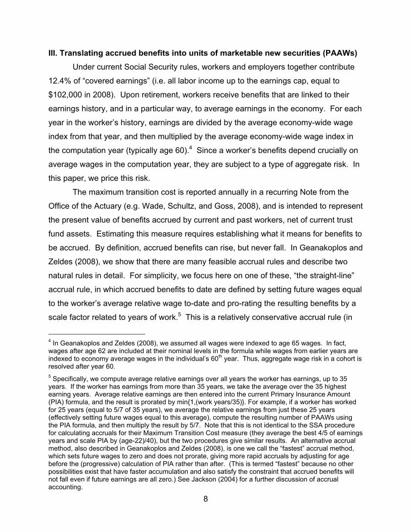
The maximum transition cost is reported annually in a recurring Note from the

Office of the Actuary (e.g. Wade, Schultz, and Goss, 2008), and is intended to represent

the present value of benefits accrued by current and past workers, net of current trust

fund assets. Estimating this measure requires establishing what it means for benefits to

be accrued. By definition, accrued benefits can rise, but never fall. In Geanakoplos and

Zeldes (2008), we show that there are many feasible accrual rules and describe two

natural rules in detail. For simplicity, we focus here on one of these, “the straight-line”

accrual rule, in which accrued benefits to date are defined by setting future wages equal

to the worker’s average relative wage to-date and pro-rating the resulting benefits by a

scale factor related to years of work.5 This is a relatively conservative accrual rule (in

4 In Geanakoplos and Zeldes (2008), we assumed all wages were indexed to age 65 wages. In fact, wages after age 62 are included at their nominal levels in the formula while wages from earlier years are indexed to economy average wages in the individual’s 60th year. Thus, aggregate wage risk in a cohort is resolved after year 60. 5 Specifically, we compute average relative earnings over all years the worker has earnings, up to 35 years. If the worker has earnings from more than 35 years, we take the average over the 35 highest earning years. Average relative earnings are then entered into the current Primary Insurance Amount (PIA) formula, and the result is prorated by min{1,(work years/35)}. For example, if a worker has worked for 25 years (equal to 5/7 of 35 years), we average the relative earnings from just these 25 years (effectively setting future wages equal to this average), compute the resulting number of PAAWs using the PIA formula, and then multiply the result by 5/7. Note that this is not identical to the SSA procedure for calculating accruals for their Maximum Transition Cost measure (they average the best 4/5 of earnings years and scale PIA by (age-22)/40), but the two procedures give similar results. An alternative accrual method, also described in Geanakoplos and Zeldes (2008), is one we call the “fastest” accrual method, which sets future wages to zero and does not prorate, giving more rapid accruals by adjusting for age before the (progressive) calculation of PIA rather than after. (This is termed “fastest” because no other possibilities exist that have faster accumulation and also satisfy the constraint that accrued benefits will not fall even if future earnings are all zero.) See Jackson (2004) for a further discussion of accrual accounting.

9

the sense of delaying accrual) and thus tends to decrease the accruals of younger

cohorts. Since these are the cohorts for whom the risk adjustment is important, this

accrual rule tends to decrease the magnitude of the overall risk-adjustment. We show

that, even with this accrual rule, the risk adjustment is quite significant.

In Geanakoplos and Zeldes (2008), we described how to create a system of

personal accounts that achieves many of the core goals of supporters of the current

system, including risk-sharing and redistribution. We called these “Progressive

Personal Accounts.” One step in that process was to show that a personal account

system could be structured to exactly reproduce the benefits promised under the current

system. This involved the creation of a new financial security, which we named a

Personal Annuitized Average Wage security, or PAAW for short. Whether or not

Progressive Personal Accounts are adopted, this equivalence means that establishing a

price for this theoretical security is sufficient for pricing existing Social Security

obligations.

We define a PAAW as a security that pays its owner one inflation-corrected dollar

for every year of his life after the year (tR) in which he hits the statutory retirement age

(R), multiplied by the economy-wide average wage (Wtc) in the computation year (tc)

that he hits age 60. PAAWs are tied to specific individuals, indexed by i, through their

mortality, the wage index in their cohort’s computation year, Wtc, and the year of the first

payout on their security (tR). In this paper, we assume all workers retire at 65, fixing the

relationship between tc and tR. In this context, the notation PAAW(i,tR) identifies the

relevant information for any PAAW.

Each additional dollar that an individual earns generates additional accrued

benefits or PAAWs. At any point in time t, an individual’s accrued benefits can be

summarized completely by the number of PAAWs owned. The present value of

accrued benefits is therefore equal to the quantity of accrued PAAWs (known at time t)

multiplied by the present value of a PAAW(i, tR).

PAAW valuations should differ for individuals in the same age cohort with

different mortality probabilities. For example, the longer life expectancies of women and

the highly educated means their PAAWs would be more valuable, if they were traded

separately. We assume that all members of a birth cohort have the same age profile of

10

survival probabilities.6 In the following sections, we examine how to price PAAWs for

each cohort, and we then estimate the quantity of PAAWs outstanding and the market

value of these PAAWS for each cohort.

IV. The price of a PAAW

In Geanakoplos and Zeldes (2008), we argued that if the Social Security system

either required workers to sell a small fraction of their PAAWs or issued extra PAAWS,

these securities could be pooled together and sold to financial markets. In this section,

we estimate what the market price of these pooled PAAWs would be if they were traded

in financial markets. To do so, we develop a valuation model that links the risk in

PAAWs to the risk in an asset which is already priced, namely stocks. We compare

this value with the value generated from the same model, but ignoring the adjustment

for risk. We refer to these respectively as the “market” (or “risk-adjusted”) and

“actuarial” (or “unadjusted”) values.7

Methodology

PAAW payouts are tied to average economy-wide wages in a specific year in the

future. They are therefore tied to the macroeconomy and potentially to the stock

market. Lucas and Zeldes (2006) show how to value defined-benefit (DB) pension

liabilities when payouts are tied to future wages of the individual. We apply that

approach here, modifying it to take into account the specifics of Social Security benefit

rules. One important difference between the two applications is that under private DB

pensions, the accrued benefit obligation (ABO) depends only on past labor earnings

(and thus requires no risk adjustment), while the projected benefit obligation (PBO)

depends on future labor earnings. Due to the wage-indexing of Social Security, even

the ABO measure of Social Security depends on future (economy-wide) labor earnings,

and therefore even the ABO measure of Social Security requires an adjustment for

salary risk.

6 To the extent that there is a correlation between life expectancy and number of accrued PAAWs, we will underestimate the value of each cohort’s accrued PAAWs. 7 A comparison of the risk adjusted and actuarial values could be used to back out an estimate of the appropriate risk-adjusted discount rate. We pursue this in Geanakoplos and Zeldes (2009).

11

The cash flow stream on a PAAW(i, tR) depends on the economy-wide average

earnings index Wtc at time tc, the lifespan of individual i, and the year of retirement tR. In

particular, an individual’s retirement benefits are an annuity proportional to the average

wage in his 60th year. If we define a wage bond as a security that pays an amount

equal to the average wage in some future year, then we can decompose the problem of

pricing a PAAW into the problem of pricing the wage bond (which requires a model of

wage growth), and pricing the annuity (which we assume is independent of wage

growth). We proceed in this manner, first pricing the wage bond, then combining our

result with a standard valuation for the cohort-specific annuity.

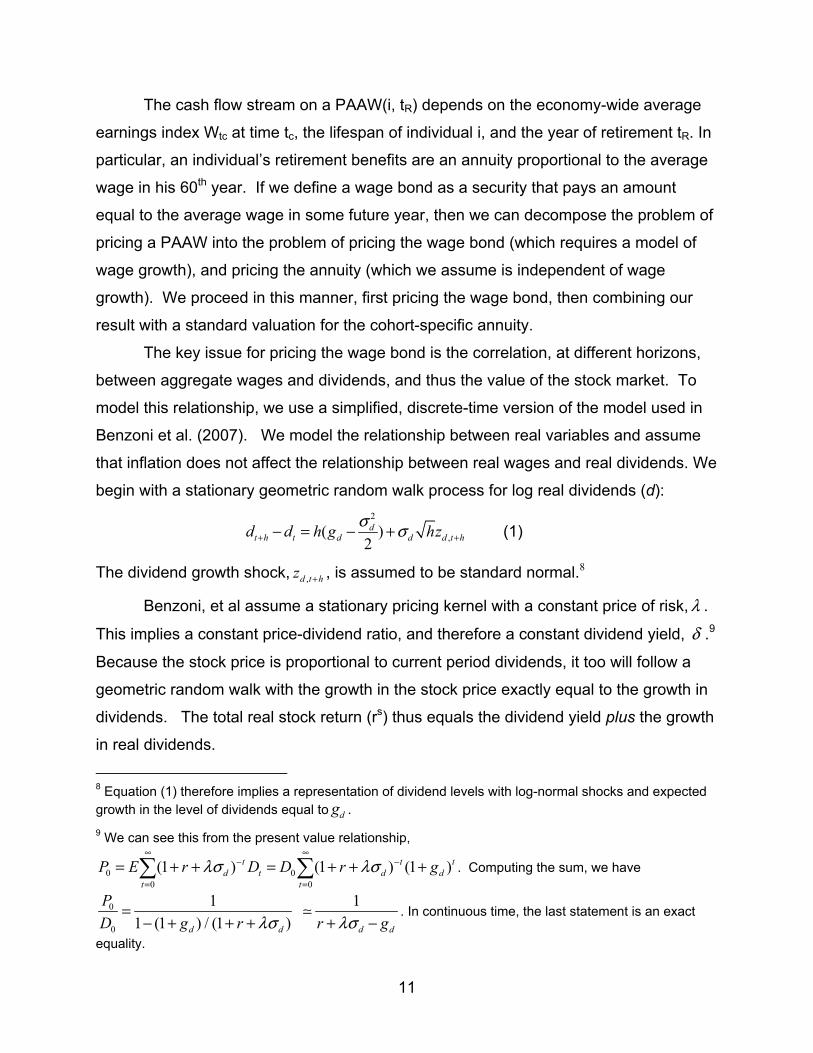
The key issue for pricing the wage bond is the correlation, at different horizons,

between aggregate wages and dividends, and thus the value of the stock market. To

model this relationship, we use a simplified, discrete-time version of the model used in

Benzoni et al. (2007). We model the relationship between real variables and assume

that inflation does not affect the relationship between real wages and real dividends. We

begin with a stationary geometric random walk process for log real dividends (d):

2

,( )2d

t h t d d d t hd zd h g hσ σ+ +− = − + (1)

The dividend growth shock, ,d t hz + , is assumed to be standard normal.8

Benzoni, et al assume a stationary pricing kernel with a constant price of risk, λ .

This implies a constant price-dividend ratio, and therefore a constant dividend yield, δ .9

Because the stock price is proportional to current period dividends, it too will follow a

geometric random walk with the growth in the stock price exactly equal to the growth in

dividends. The total real stock return (rs) thus equals the dividend yield plus the growth

in real dividends.

8 Equation (1) therefore implies a representation of dividend levels with log-normal shocks and expected growth in the level of dividends equal to gd .

9 We can see this from the present value relationship,

00 0

0 (1 (1 (1) ) )t t td t d d

t t

P rE Dr D gλσ λσ∞ ∞

− −

= =

+ + = + + += . Computing the sum, we have

0

0

1 11 (1 (1

/ ))d d d d

PD g r r gλσ λσ

=− + + + + −

. In continuous time, the last statement is an exact

equality.

12

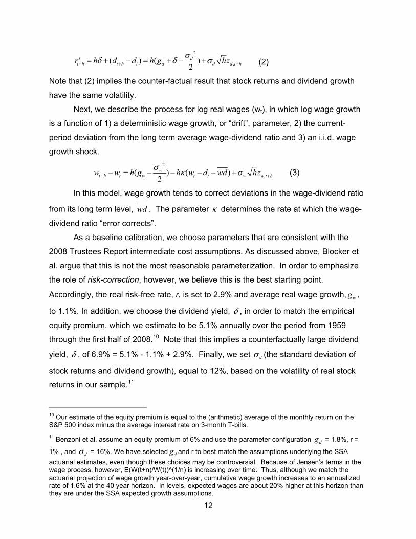
2

,( (2

) )s dt h t h t d d d t hd d h g hzr h σδ δ σ+ + += =+ − + − +

(2)

Note that (2) implies the counter-factual result that stock returns and dividend growth

have the same volatility.

Next, we describe the process for log real wages (wt), in which log wage growth

is a function of 1) a deterministic wage growth, or “drift”, parameter, 2) the current-

period deviation from the long term average wage-dividend ratio and 3) an i.i.d. wage

growth shock.

2

,( ) ( )2t h t w t t w t hw

ww h g h w d wd hzw σ κ σ+ +− = − +− − − (3)

In this model, wage growth tends to correct deviations in the wage-dividend ratio

from its long term level, wd . The parameter κ determines the rate at which the wage-

dividend ratio “error corrects”.

As a baseline calibration, we choose parameters that are consistent with the

2008 Trustees Report intermediate cost assumptions. As discussed above, Blocker et

al. argue that this is not the most reasonable parameterization. In order to emphasize

the role of risk-correction, however, we believe this is the best starting point.

Accordingly, the real risk-free rate, r, is set to 2.9% and average real wage growth, wg ,

to 1.1%. In addition, we choose the dividend yield, δ , in order to match the empirical

equity premium, which we estimate to be 5.1% annually over the period from 1959

through the first half of 2008.10 Note that this implies a counterfactually large dividend

yield, δ , of 6.9% = 5.1% - 1.1% + 2.9%. Finally, we set dσ (the standard deviation of

stock returns and dividend growth), equal to 12%, based on the volatility of real stock

returns in our sample.11

10 Our estimate of the equity premium is equal to the (arithmetic) average of the monthly return on the S&P 500 index minus the average interest rate on 3-month T-bills.

11 Benzoni et al. assume an equity premium of 6% and use the parameter configuration dg = 1.8%, r =

1% , and dσ = 16%. We have selected dg and r to best match the assumptions underlying the SSA

actuarial estimates, even though these choices may be controversial. Because of Jensen’s terms in the wage process, however, E(W(t+n)/W(t))^(1/n) is increasing over time. Thus, although we match the actuarial projection of wage growth year-over-year, cumulative wage growth increases to an annualized rate of 1.6% at the 40 year horizon. In levels, expected wages are about 20% higher at this horizon than they are under the SSA expected growth assumptions.

13

From the perspective of this paper, the most important parameter calibration is

our choice of κ . Benzoni et al (2007) estimate κ to be between .05 and .2, and take

0.15 as their baseline value, which we follow in this paper. We also examine the

robustness of our results to different values of κ .

Following Lucas and Zeldes (2006), we assume that all risk not captured by the

relationship between wages and stocks would be priced by the market at zero, and we

use risk-neutral Monte Carlo derivative pricing techniques (as in Cox, Ross, Rubenstein

1979) to price a wage bond as a derivative on the stock market. This entails generating

a set of hypothetical “risk-neutral” probabilities on the set of possible returns for stocks

such that, under those probabilities, the expected return would equal the risk-free rate.

In our simple model, this “risk-neutral” distribution for stock returns is normal with a

mean equal to the risk-free rate and the standard deviation equal to its original empirical

value.

We use Monte-Carlo techniques to simulate stock returns and wages using the

risk-neutral probabilities. We generate 200,000 replications of the wage and dividend

process, each 45 years in length, and take averages over the realizations. Our estimate

of the “risk-adjusted” price of a year-t wage bond is equal to the average value of the

simulated wage at year t, using risk-neutral probabilities, discounted at the risk-free rate.

We use the wage bond price to compute the current market value of a PAAW. A

PAAW for this worker promises payments proportional to the age 60 average wage,

starting in the retirement year, which we assume to be age 65. To compute annuity

prices, we use the cohort life tables from Bell and Miller (2002) and assume that all

individuals of the same age face the same conditional survival probabilities12, i.e. that

there is no heterogeneity or private information about these probabilities. We also

assume that the market price of aggregate longevity risk and inflation risk are each

zero.

As a concrete example of how we compute PAAW prices, consider the cohort of

age 50, which reaches age 60 in 2015, ten years from our valuation date. We compute

the risk-adjusted value in 2005 of the 2015 wage bond to be 0.658 current wage units.

12 For the calculations presented, we used the survival probabilities for males born in 1980. Using sex-specific survival probabilities increases our measure of accrued benefits by about 7% (since women typically live longer than men). The combined risk-adjustment, however, is only negligibly affected.

14

The age 60 value of a one-dollar perpetual real annuity starting at age 65, valued using

cohort-specific mortality and a risk-free rate, is $10.88. Finally, conditional on being 50

years old in 2005, there is a 92.3% chance of reaching age 60, the year we value the

annuity. Therefore, the 2005 value of a PAAW for this cohort is (10.88) * (0.658) *

(0.923) = 6.60 current wage units. Multiplying by the current value of the average wage

gives the dollar-value of a PAAW.

Actuarial value

The standard actuarial approach for computing present value makes no

adjustment for risk, i.e. it computes the expected value of the cash flows and discounts

at the risk-free rate.13 To estimate the “non-risk-adjusted” or actuarial price of a wage

bond, we use the same model described above, but generate a set of wage and

dividend realizations that are based on the true probabilities, and then discount the

average value of the simulated wage at the risk-free rate.

Results

Figure 1 compares the actuarial and market prices of the wage bonds. The risk

adjustment causes the market price to be everywhere lower than the actuarial price. In

addition, the difference grows over time, since wages further out are more risky and

subject to a larger adjustment.14

Figure 2 compares the actuarial prices of PAAWs and the risk-adjusted market

price of PAAWs. Figure 3 shows the ratio of market (risk-corrected) to actuarial PAAW

prices for each cohort. For cohorts that have already surpassed the computation age

(60), the risk-adjustment has no impact on the valuation. This occurs because

aggregate wages are the only source of priced risk in our model, and cohort benefits

depend on aggregate wages in the year it turns 60. For younger cohorts, however,

there is a significant difference between the two methods. For cohorts under age 40,

13 Note that if all individuals in the economy were risk-neutral, no adjustment for risk would be necessary, and the actuarial and market approaches would yield identical results. 14 Both prices decrease with the horizon, reflecting the fact that the risk-free rate is greater than average wage growth. In addition, both prices are slightly less than one in the initial 2005 period due to our assumption that cash flows occur at the end of each period and are discounted back to the beginning of the period.

15

the risk-adjusted measure is less than half of the actuarial valuation. For the youngest

cohorts we consider (age 20 in 2005) adjusted accruals are worth less than 20% of their

value under the standard approach.

V. The quantity of PAAWs outstanding

In this section, we estimate the stream of future benefits that have been accrued

by each cohort based on contributions to date. As pointed out above, these can be

neatly described with a single summary statistic: the number of PAAWs accrued by the

cohort.

To construct accrual, we use data from the Continuous Work History Sample

(CWHS), a 1% sample of workers and beneficiaries.15 The key feature of this dataset,

for our purposes, is that it includes individual-specific earnings histories.16 We compute

accrued benefits for both current and former workers (including retirees). For retirees

this simply entails averaging the 35 years of highest relative earnings and entering this

average into the PIA formula (redefined to be in units of future economy-wide wages).

For workers who have not already retired, we use the straight-line accrual formula

described above to compute PAAW accruals based on worker earnings histories to

date. Because our dataset has no information on spousal earnings or status, our

results ignore any potential spousal or survivor benefits. The quantity of PAAWs

accrued to date by a cohort is equal to the sum of the PAAWs accrued to date by all

individuals in the cohort.

Estimates of PAAW quantities by cohort

Figure 4 shows our estimate of PAAWs earned through 2004 for cohorts born

between 1910 and 1986 (ages 19 through 95 in 2005). The hump shape in quantities

reflects three key features of benefit accruals and Social Security demographics: 1)

younger cohorts have shorter work histories and thus have accrued fewer benefits, 2)

15 We are grateful to Jae Song and Wojciech Kopczuk for providing us with summary statistics from the CWHS. 16 Earnings occurring before 1951 are treated differently in this dataset and are typically available only as single entry summing all earning from 1950 and earlier. We ignore these earnings entirely, meaning we slightly underestimate benefits for the oldest cohorts we consider. Because the benefit formula allows workers to exclude low earnings years, typically early years in a worker’s history, our underestimate should be very small.

16

the middle aged cohorts are large and have already accrued most of their benefits, and

3) older cohorts have fewer members because of mortality (for example, in 2005 there

were 3.6 million living individuals aged 55 but only 2.3 million aged 65 and 1.7 million

aged 75).

VI. The market value of accrued benefits

Once we have computed the price of a PAAW for each cohort and the quantity of

PAAWs outstanding for each cohort, estimating the market value of accrued benefits

simply involves multiplying the two and summing across cohorts. Figure 5 compares

the risk-adjusted and the actuarial valuations by cohort. As with the wage bond prices

in Figure 1, the risk-adjustment reduces the value of the liability for all of the non-retired

cohorts. Differences across cohorts of the adjustment suggest that risk-correction

should be a key consideration in evaluating the “fairness” of proposals to reform Social

Security.

Table 1 sums accrued benefits across cohorts for an estimate of the total value

of accrued benefits. We present two estimates: an actuarial valuation and a risk-

adjusted valuation. Our estimate of total accrued benefits, based on the actuarial

valuation methodology, is just under $13 trillion. Adjusting the Office of the Actuary’s

own 2005 estimate of accrued benefits for comparability gives a value of $12.2 trillion.17

Given our lack of information about benefits other than basic retirement benefits paid to

primary beneficiaries, our estimate of accruals without risk adjustment comes

remarkably close to SSA figures.18

17 Our estimate from CWHS data includes only “own-history” accruals, i.e. it excludes spousal and survivor benefits. To obtain a comparable estimate from SSA publications we start with the January 1, 2006 value of the Maximum Transition Cost of $15.8 trillion, which is the present value of accruals less the amount of the Social Security Trust Fund (Wade, Schultz, and Goss, 2008). To this we add back the December 31, 2005 value of the OASDI Trust Fund of $1.86 trillion (Social Security Administration, 2007). We then multiply this sum by the percentage of benefits paid to retired workers based on their own earnings history, which was roughly 70% in 2005 (Social Security Administration, 2006). To make this adjustment, we assume that the proportion of benefits going to disability and survivors is constant across cohorts and over time. This implies that these programs represent a constant proportion of accrued benefits as well. 18 In principle our actuarial estimate should match the adjusted SSA figure. Differences may arise for at least 3 reasons: 1) Our limited information does not allow us to perfectly adjust SSA figures derived from micro models. To make this adjustment, we make the simplifying assumption that the proportion of benefits going to spouses, survivors and disabled beneficiaries is constant across cohorts and over time. 2) The “straight-line” accrual formula we use is slightly different than the one used by SSA to compute the MTC measure, principally because SSA excludes some years of low earnings in estimating PIA, even for

17

We estimate a market value for the same liability of $10.5 trillion, only 81% of the

actuarial value.19 This difference in valuation comes entirely from the risk-correction; all

other features of the pricing model are held constant in generating the figures. This

suggests that the standard approach of discounting expected future benefits by the risk-

free rate is significantly overstating the size of accrued benefits. Appropriately

correcting for risk to aggregate wage growth reduces our measure of Social Security

benefits obligations by nearly 20%. Subtracting the end of 2005 value of the OASI trust

fund (1.66 trillion) from both measures indicates that the market value estimate of the

maximum transition cost measure of Social Security’s financial status is only 78% as

large as the actuarial value, suggesting a healthier system (in the sense of ease of

transition to an alternative system) than found using traditional actuarial methods.

Table 1 also breaks down the liability for cohorts below age 60, and those 60 and

above. Age 60 is key because that is the year by which the wage risk to benefits is

resolved. For the 60-and-over group, the actuarial and risk-adjusted estimates are

identical, and the aggregate numbers reflect this. When we examine the pre-60 year-

old group alone, however, we see significantly larger differences between the actuarial

and risk-adjusted estimates: correcting for risk reduces our measure of Social Security

benefits obligations for those under 60 by nearly 30%.

VII. Robustness

The parameter κ plays a key role in our analysis because it governs the strength of the

link between wages and the stock market. Our baseline calibration follows Benzoni et

al (2007) in setting this parameter to .15. However, because of the difficulty in

estimating such cointegrating relationships, it is informative to examine the sensitivity of

workers who have yet to reach 35 years of earnings, while we do not (see footnote 5). 3) Expected long-term growth in wages differs from SSA projections, as described in footnote 11. 19 This differs from an earlier (2007) draft of this paper for three reasons. First, in this version we have linked retirement benefits to wages at age 60 (as opposed to age 65 in the earlier draft), effectively removing 5 years of risk from every cohort. This is appropriate because, as noted earlier, the age 60 wage index is used in computing benefits. Second, in this version, we use the straight-line method of accrual, instead of the “fastest” method used in the earlier draft. We choose this because it more closely matches the measure used by the Office of the Actuary to compute the maximum transition cost estimates. It implies lower current accruals for non-retired workers – those for whom the risk adjustment matters. Under fastest accrual, the corresponding adjustment is 22%. Finally, in this draft we are using revised estimates from the 2005 CWHS, whereas in the previous version we used two sources: the 2004 CWHS and a set of OASDI benefit expenditure projections provided by the SSA Office of the Actuary.

18

our results to this parameter. To do this, we perform the same simulation with a high

(.25) and a low (.05) value for κ . Figure 6 shows the ratio of the risk-adjusted price to

the actuarial price for PAAWs under the alternative calibrations.

First, we find, not surprisingly, that the importance of risk correction varies

directly with κ : higherκ implies that wage growth is more “exposed” to stock market

risk and increases the size of the risk adjustment.

In addition, we see in Figure 6 that the size of the risk correction varies in a non-

linear way with κ . For all cohorts, increasing κ from a low value of .05 to our baseline

value of .15 has a large effect on the ratio of market to actuarial value, whereas further

increasing κ from the baseline to a value of .25 has a much smaller effect.

Finally, the impact of varying κ differs across cohorts. Define the risk adjustment

as the distance as measured down from the dashed line. The percentage change in

this risk adjustment in response to changing κ is lower for the older cohorts than it is for

the younger cohorts. Consider the 50-year old cohort as an example. The adjustment

represents under 1% of the actuarial value under the “low κ ” parameterization, but 27%

of the actuarial value under the “high κ ” parameter choice. In contrast, for the 20-year-

old cohort, the adjustment is large even for low κ , and raising κ results in a much

smaller percentage increase in the adjustment than it did for the 50-year old cohort.

This pattern is natural; in our model, the long-run correlation between wages and the

stock market is 1 for any κ greater than 0, even a small value. Thus the risk adjustment

for benefits far in the future will be (essentially) independent of the parameter κ . On

the other hand, the shorter-run correlation between wages and the stock market is

highly dependent on κ , so that the risk adjustment of the benefits of workers closer to

retirement is much more sensitive to the value of κ .

Table 2 aggregates the results across cohorts and examines how they change as

κ varies. Increasing κ from the baseline of .15 to .25 increases the risk correction by

only 4 percentage points (from 19% to 23%). On the other hand, lowering κ from .15 to

.05 decreases the risk adjustment by 8 percentage points (from 19% to 11%), a much

larger amount. The risk-adjustment remains important, however, even with this weak

link between wages and stock prices.

19

VIII. Conclusions, policy implications, and future research

We have argued that market value is the appropriate way to measure both the

assets and the liabilities of the Social Security system. Market value calculations adjust

for risk and differ in important ways from the standard actuarial approach that discounts

expected cash flows with a risk-free rate. We estimate that adjusting for risk reduces

the present value of accrued benefits of the entire system by about 20% and of workers

under age 60 by about 30%.

In ongoing work (Geanakoplos and Zeldes, 2009), we extend this approach to

consider other measures of Social Security’s financial status, including open group

measures that incorporate both future Social Security contributions and the

corresponding future accruals. Since future tax contributions are proportional to wages

(up to the earnings cap), they are subject to a similar risk correction. For the measure

we study here, where only future benefit flows must be valued, the direction of the risk

adjustment effect is unambiguous; Social Security obligations are worth less under

market valuation. Once we consider adjusting both the assets (future taxes) and the

liabilities of Social Security (including future accruals), the picture becomes significantly

more complicated, and preliminary results suggest that the market value of open group

measures shows a larger deficit than the actuarial value.

20

References

Bell, Felicitie C. and Michael L. Miller. 2002. “Life Tables for the United States Social

Security Area 1900-2100.” Social Security Administration, Actuarial Study No. 116.

Benzoni, L, P. Collin Dufresne, and R. Goldstein. 2007. "Portfolio Choice over the Life-

Cycle when the Stock and Labor Markets are Cointegrated." Journal of Finance, Vol 62, No 5, October.

Blocker, Alexander W., Laurence J. Kotlikoff, and Stephen A. Ross. 2008. “The True

Cost of Social Security,” NBER Working Paper No. 14427, October. Cox, John C., Ross, Stephen A. Ross and Mark Rubenstein. 1979. “Option Pricing: A

Simplified Approach.” Journal of Financial Economics Vol 7, September: 229-263.

Federal Accounting Standards Advisory Board. 2006. "Accounting for Social Insurance,

Revised – Statement of Federal Financial Accounting Standards.” Available at http://www.fasab.gov/pdffiles/socialinsurance_pv.pdf , October.

Federal Accounting Standards Advisory Board. 2009. "Accounting for Social Insurance,

Revised.” Available at http://www.fasab.gov/exposure.html. Geanakoplos, John, Olivia Mitchell, and Stephen P. Zeldes. 1999. “Social Security

Money’s Worth.” in Prospects for Social Security Reform, ed. Olivia S. Mitchell, Robert J. Meyers, and Howard Young. Philadelphia: Pension Research Council, University of Pennsylvania Press.

Geanakoplos, John, and Stephen P. Zeldes. 2008. “Reforming Social Security with

Progressive Personal Accounts.” NBER Working Paper # 13979. Forthcoming in Social Security Policy in a Changing Environment, ed. Jeffrey Brown, Jeffrey Liebman and David A. Wise. Chicago: University of Chicago Press.

Geanakoplos, John, and Stephen P. Zeldes. 2009. “The Market Value of Social

Security.” Unpublished manuscript, Columbia University Graduate School of Business.

Goetzmann, William N. 2008. “More Social Security, Not Less.” Journal of Portfolio

Management, Fall, Vol. 35, No 1: 115-123. Jackson, Howell. 2004. “Accounting for Social Security and Its Reform.” Harvard

Journal on Legislation, Vol. 41, Number 1, Winter: 59-159. Lucas, Deborah and Stephen P. Zeldes. 2006. “Valuing and Hedging Defined Benefit

Pension Obligations - The Role of Stocks Revisited.” Unpublished manuscript, Columbia University Graduate School of Business, September.

21

Social Security Administration. 2008. The 2008 Annual Report of the Board of Trustees

of the Federal Old-Age and Survivors Insurance and Federal Disability Insurance Trust Funds. Table II.C.2. Washington, DC: Office of Policy. http://www.socialsecurity.gov/OACT/TR/TR08/trLOT.html

Social Security Administration. 2006. Annual Statistical Supplement to the Social

Security Bulletin, Table 5.A1. Washington, DC: Office of Policy. http://www.socialsecurity.gov/policy/docs/statcomps/supplement/2006/5a.html

Technical Panel. 2007. Report on Assumptions and Methods. Report to the Social

Security Advisory Board, October. http://www.ssab.gov/documents/2007_TPAM_REPORT_FINAL_copy.PDF

Wade, Alice, Jason Schultz, and Steve Goss. 2008. “Unfunded Obligation and

Transition Cost for the OASDI Program.” Actuarial Note #2008.1, Social Security Administration, Office of the Chief Actuary, July.

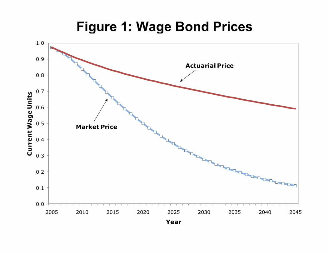
Figure 1: Wage Bond Prices1.0

0.8

0.9Actuarial Price

0.6

0.7

e U

nit

s

0.4

0.5

ren

t W

age

Market Price

0.2

0.3Cu

rr

0.0

0.1

2005 2010 2015 2020 2025 2030 2035 2040 2045

Year

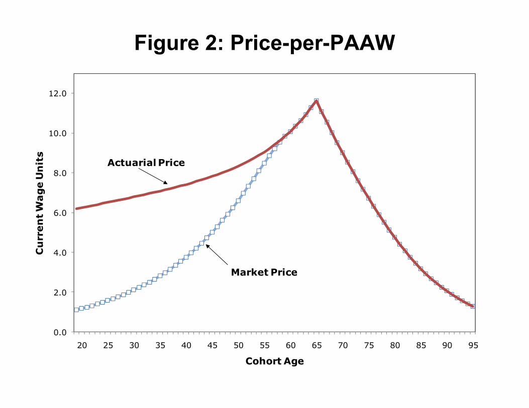
Figure 2: Price-per-PAAW

12.0

8.0

10.0

Un

its

Actuarial Price

6.0

en

t W

ag

e U

4.0Cu

rre

Market Price

0 0

2.0

0.095908580757065605550454035302520

Cohort Age

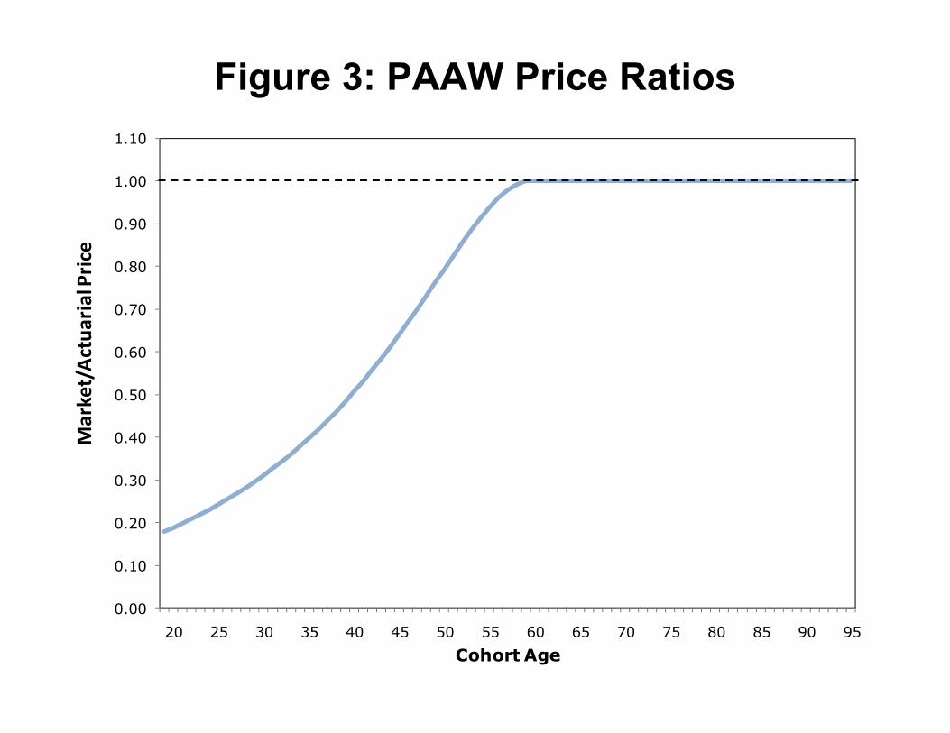
Figure 3: PAAW Price Ratios 1 10

0.90

1.00

1.10

0.70

0.80

0.90

rial Price

0.50

0.60

rket/Actua

0.30

0.40Mar

0.10

0.20

0.0095908580757065605550454035302520

Cohort Age

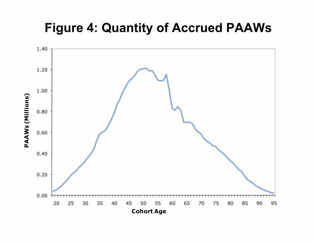
Figure 4: Quantity of Accrued PAAWs

1.20

1.40

1.00

on

s)

0.60

0.80

AW

s (M

illi

o

0.40

PA

A

0.00

0.20

0 0095908580757065605550454035302520

Cohort Age

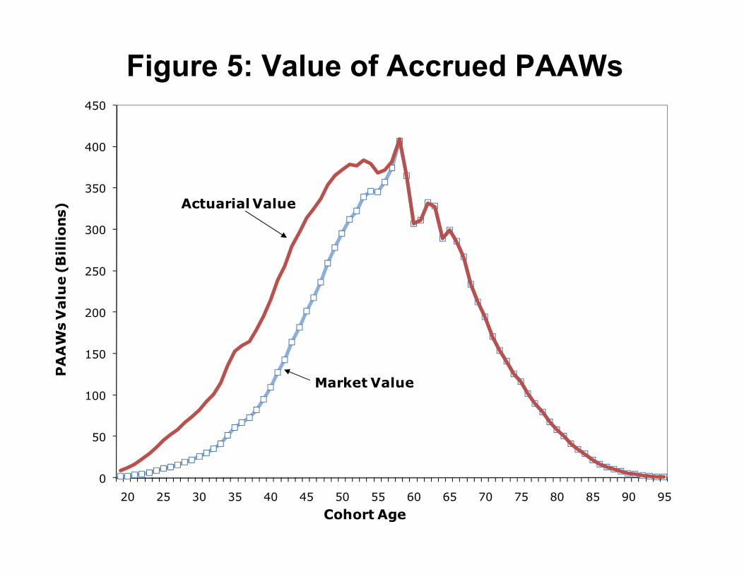
Figure 5: Value of Accrued PAAWs450

400

450

300

350

llio

ns)

Actuarial Value

200

250

s V

alu

e (

Bi

100

150

PA

AW

s

Market Value

50

100

095908580757065605550454035302520

Cohort Age

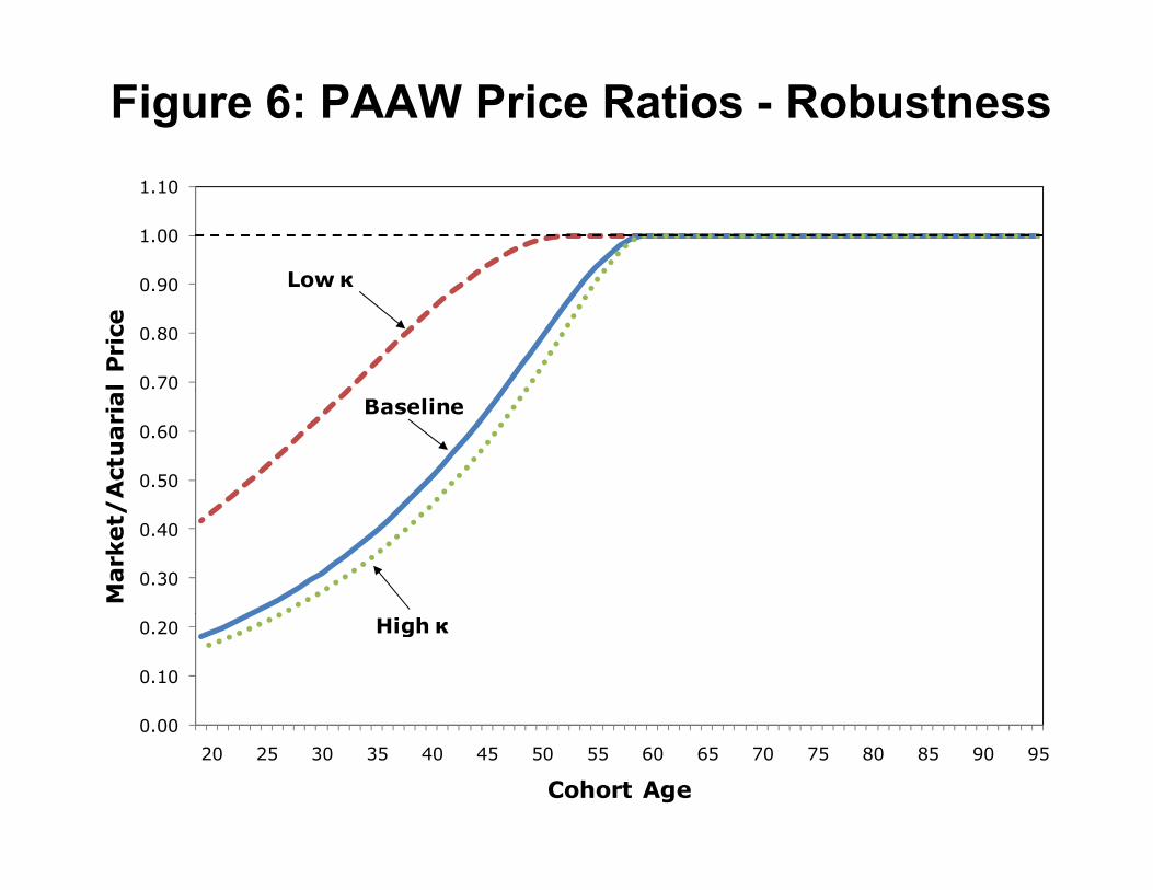
Figure 6: PAAW Price Ratios - Robustness

1.00

1.10

Low κ

0.70

0.80

0.90

l P

rice

Low κ

0.50

0.60

0 0

/A

ctu

ari

al

Baseline

0.30

0.40

Mark

et/

0 00

0.10

0.20 High κ

0.0095908580757065605550454035302520

Cohort Age

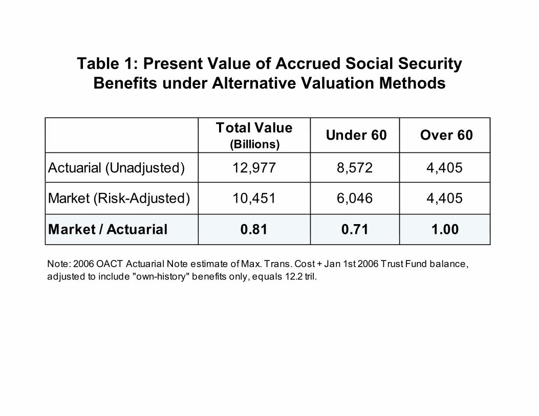
Table 1: Present Value of Accrued Social Security B fi d Al i V l i M h dBenefits under Alternative Valuation Methods

Total ValueTotal Value (Billions)

Under 60 Over 60

Actuarial (Unadjusted) 12,977 8,572 4,405

Market (Risk-Adjusted) 10,451 6,046 4,405

Market / Actuarial 0.81 0.71 1.00

Note: 2006 OACT Actuarial Note estimate of Max. Trans. Cost + Jan 1st 2006 Trust Fund balance, adjusted to include "own-history" benefits only, equals 12.2 tril.

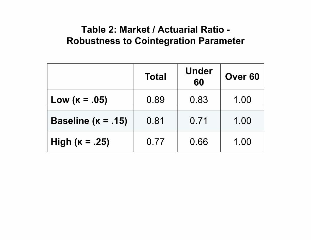
Table 2: Market / Actuarial Ratio -Robustness to Cointegration Parameter g

T t lUnder

O 60Total60

Over 60

Low (κ = .05) 0.89 0.83 1.00

Baseline (κ = .15) 0.81 0.71 1.00

High (κ = .25) 0.77 0.66 1.00