This work is distributed as a Discussion Paper by the

STANFORD INSTITUTE FOR ECONOMIC POLICY RESEARCH

SIEPR Discussion Paper No. 07-50

Marrying Up: the Role of Sex Ratio in Assortative Matching

By Ran Abramitzky

Stanford University

Adeline Delavande

Universidade Nova de Lisboa

Luís Vasconcelos

Universidade Nova de Lisboa

July 2008

Stanford Institute for Economic Policy Research

Stanford University

Stanford, CA 94305

(650) 725-1874

The Stanford Institute for Economic Policy Research at Stanford University supports research bearing on

economic and public policy issues. The SIEPR Discussion Paper Series reports on research and policy

analysis conducted by researchers affiliated with the Institute. Working papers in this series reflect the views

of the authors and not necessarily those of the Stanford Institute for Economic Policy Research or Stanford

University.

Marrying Up: the Role of Sex Ratio in Assortative Matching*

Ran Abramitzky Adeline Delavande Luís Vasconcelos Stanford University Universidade Nova de Lisboa

and Rand Corporation Universidade Nova de Lisboa

July 2008

Abstract We investigate the effect of a change in the sex ratio on assortative matching in the marriage market using a large negative exogenous shock to the French male population due to WWI casualties. We analyze a novel data set that links marriage-level data to both French censuses of population and regional data on military mortality. We instrument the potentially endogenous sex ratio with military mortality, which exhibits exogenous geographic variation. We find that men married women of higher social class than themselves (married up) more in regions that experienced a larger decrease in the sex ratio due to higher military mortality. A decrease in the sex ratio from one man for every woman to 0.90 men for every woman increased the probability that men married up by 8.2 percentage points. These findings shed light on individuals’ preferences for spouses. Rather than preferring to marry spouses with similar characteristics, individuals seem to prefer to marry higher-class spouses, but cannot do so when the sex ratio is balanced.

JEL Code: J12, N34 Keywords: Marriage, sex ratio, assortative matching, social classes.

* We thank Pedro P. Barros, Effi Benmelech, Marianne Bertrand, Nick Bloom, Leah Boustan, Tim Bresnahan, Raj Chetty, Dora Costa, Giacomo De Giorgi, Liran Einav, Marcel Fafchamps, Amy Finkelstein, Iliyan Georgiev, Avner Greif, Tim Guinnane, Christina Gathmann, Caroline Hoxby, Murat Iyigun, Seema Jayachandran, Naomi Lamoreaux, Michael Lovenheim, Victor Lavy, Soo Lee, Pierre-Carl Michaud, José Mata, Joel Mokyr, Muriel Niederle, Ben Olken, John Pencavel, Luigi Pistaferri, Gilles Postel-Vinay, Jean-Laurent Rosenthal, Emmanuel Saez, Izi Sin, Neeraj Sood, Nathan Sussman, Michele Tertilt, Gui Woolston, Yoram Weiss, Gavin Wright, and participants in numerous seminars and conferences for helpful discussions and comments. We thank Jean-Pierre Pélissier for kindly providing us with the marriage-level data from the TRA data set. We are grateful to Izi Sin for superb research assistance.

1

I. Introduction

Positive assortative matching in the marriage market by spouses’ characteristics such as

income, education, occupation, age, religion, and ethnicity is a well-known and widespread

phenomenon (e.g., Hout 1982, Mare 1991, Kalmijn 1998, Blossfeld and Timm 2003).1 Moreover, the

tendency of individuals to marry others with similar traits has important implications for social

inequality, income redistribution, fertility, education, and labor supply (e.g., Fernandez and Rogerson

2001). However, there is still little understanding about what generates this assortative matching. One

possibility is that individuals have horizontal preferences. That is, they may choose spouses who share

similar characteristics simply because they derive more utility from marrying people like themselves.2

Alternatively, individuals may have vertical preferences, meaning they prefer to marry “up,” i.e. to

marry someone exhibiting better characteristics (such as higher income or higher education), but

cannot, because they do not receive marriage proposals from such people.3 Finally, individuals may

have the opportunity to meet only people who share their characteristics. We use unique data on a

negative exogenous shock to the male population to investigate which of these preferences and

constraints are responsible for assortative matching, or marriage by “class.”

Identifying which of the above mechanisms underlies the equilibrium matching outcomes in the

marriage market is challenging: they all generate observationally equivalent outcomes, i.e. assortative

matching whereby people marry by “class.” Our identification strategy relies on the fact that under

different preferences an exogenous change in the sex ratio has a different impact on equilibrium

marriage outcomes. Specifically, if individuals marry by class because they intrinsically prefer a

spouse with similar characteristics, or because they only meet potential partners with the same

background, an exogenous decrease in the proportion of men in the population would have a limited

effect on the assortative matching: men would continue to marry women of the same class. If instead

individuals prefer spouses of higher class than themselves, the same decrease in the proportion of men

would improve the position of men in the marriage market and eventually enable them to marry

women from higher classes who were previously inaccessible.

We exploit the regrettable fact that World War I (WWI), one of the deadliest conflicts in recent

human history, produced an exogenous and unusually large shock in the French male population.

1 See Pencavel (1998) and Rose (2001) for trends in assortative matching in the U.S. 2 Aristotle noted that people “love those who are like themselves” (Aristotle 1934, p. 1371). Sociologists believe that “the homophily principle structures network ties of every type, including marriage, friendship, work, advice, support, information transfer, exchange, comembership, and other types of relationship” (McPherson, Smith-Lovin, and Cook 2001). 3 See, for example, Burdett and Coles (1997).

2

Approximately 16.5% of French soldiers were reported dead or missing after the war (Huber, 1931).

The First World War in France provides an ideal setting to test the effect of the sex ratio on marriage

by social class for the following reasons. First, the ratio of men aged 18 to 59 to women aged 15 to 49

decreased from 1,087 men per 1,000 women in 1911 to 992 men per 1,000 women in 1921 in an

exogenous way as a result of the military mortality.4 Second, military mortality varied substantially

across regions, ranging from 5% to 23% of men aged 18 to 59 (see Figure 1.1), largely because of

different regiment call-ups. This variation generated substantial heterogeneity in sex ratios across

regions, reaching 864 men per 1,000 women in some regions, allowing us to precisely evaluate the

impact of the sex ratio on assortative matching. Finally, unlike in many other wars, military mortality

was uniform across occupations, which we use to define social class, implying that the distribution of

social classes in the population remained essentially unchanged by the war (see Table 1.1). This fact

rules out the hypothesis that changes in marriage by class following the war were mechanically driven

by changes in the distributions of classes.

We analyze the impact of this massive decrease in the male population on marriage by social

class in France using a new data set which links marriage-level data to both French censuses of

population and regional data on military mortality. Classes are assigned to individuals using marriage

certificate data that provide information on the occupations of the brides, grooms, and their parents, as

well as the place and date of each marriage. Based on either the occupations of the bride and groom or

the occupations of their fathers, we allocate individuals into seven ordered social classes using the

Historical International Social Class Scheme (HISCLASS) developed by van Leeuwen and Maas

(2005a). These social classes, based on dimensions such as the degree of supervision required to

perform the job, the skill level required, whether the job is manual or not, and the economic sector,

were carefully constructed to categorize individuals according to their life chances. There was

considerable assortative matching by social class before WWI: 43% of men married women of the

same social class, and the distance between the social classes of spouses was 1 or less for 68% of

couples. Based on the locations of the marriages, we link the marriage-level data with the French

censuses of 1911, 1921 and 1926. These contain region-level information that allows us to construct

the sex ratio for all the French départements (regional unit), as well as other département-level control

variables.5 We also use military mortality data from the French ministry of defense to compute, for

4 Since this war was fought in the battlefield, civilian mortality (which is more balanced across genders) was lower than in later major wars such as the Second World War. 5 Departments are administrative units similar to counties. In 1870-1914, France had 87 départements. After WWI, the number increased to 90 because territories from Alsace-Lorraine lost in the 1870s were recovered.

3

each département, the military mortality rate corresponding to the number of dead soldiers as the

percentage of the pre-war male population.

We use two empirical strategies to analyze the effect of a change in the sex ratio. First, we

compare the distribution of brides’ classes for each class of groom before and after the war. Second,

we exploit the exogenous regional variation in sex ratio due to war mortality to investigate more

directly the relationship between sex ratio and marriage outcomes. We use three alternative dependent

variables to capture whether and to what degree men married women of higher classes (i.e., married

up), namely (i) the difference between the social class of the bride and that of the groom; (ii) a dummy

for whether the groom married a bride of higher class than his; and (iii) a dummy for whether the

groom married a bride of low social class, meaning a bride in one of the three lowest classes according

to HISCLASS classification. As alternative independent variables of interest we use département-

specific sex ratios and mortality rates. We also use mortality rates as an instrument for sex ratio, which

may be endogenous because of the possible selection of internal migrants.

We include département fixed effects to control for permanent differences between French

départements, and also include a time trend. The analysis also controls for other marriage-level

characteristics that might affect assortative matching such as the groom’s class, the spouses’ ages, and

whether the marriage took place in a rural area. In addition, we control for the contemporaneous

distribution of women’s occupations to account for possible changes in the labor force due to the war,

as well as for the excess of foreign men over foreign women, to account for the possibility that foreign

men (mainly Italians) migrated to France after the war and competed with French men for local brides.

Overall, we find that the decrease in sex ratio caused by war-related mortality allowed men to

marry higher class women. Specifically, a decrease in the (instrumented) sex ratio from one man for

every woman to 0.90 men for every woman corresponds to (i) an increase in the average class of bride

for a given class of groom of 0.27, meaning for instance that if class 4 men married on average class 4

women when the sex ratio was even, they would marry on average class 3.73 women under a 0.90-to-1

sex ratio; (ii) an increase in the probability that men would marry women of (weakly) higher class than

themselves of 8.2 percentage points; and (iii) a decrease in the probability that a given groom would

marry a low class bride of 18.5 percentage points. As a robustness check, we test whether the effect of

sex ratio on assortative matching is different in rural locations, where search frictions, meeting

technology and preferences might be different compared with urban locations. We find a similar effect

of sex ratio in rural and urban areas.

We view these findings as evidence that on average individuals prefer higher-class partners. This

favors the hypothesis that assortative matching occurs because in equilibrium individuals cannot marry

4

higher-class people, although they may wish to do so. In addition, we find heterogeneity in the effect

of the sex ratio by groom’s class, with men of the lowest classes, namely low-skilled and unskilled

farm workers, benefiting the least from the sex ratio imbalance. A possible explanation is that while

high and middle-class women were willing to marry men from lower social classes, they were not

willing to accept proposals from men of very low social class.

While the main focus of this paper is assortative matching by social class, there are clearly

other dimensions of “attractiveness” individuals consider when choosing a spouse. Our data allow us

to study assortative matching by another important such dimension, namely age. Specifically, we

investigate whether the decrease in sex ratio due to war mortality changed the spousal age gap. We

employ the same empirical strategies described above, and find a higher decrease in the age gap

between grooms and brides in départements with higher mortality. Given that grooms are, on average,

older than their brides, these results are consistent with men preferring women who are closer to their

own age.

Starting with the seminal work of Becker (1973, 1974), economists have devoted considerable

attention to understanding marriage markets.6 In particular, an important issue in the empirical

literature of the marriage market has been the characterization of individuals’ preferences for spouses.

This characterization is difficult because equilibrium outcomes in the marriage markets are not only

determined by preferences, but also by the mechanisms that match men and women. One strand of the

literature deals with the identification problem by performing structural estimations of marriage

models using marriage outcomes data (e.g., Wong 2003, Bisin et al. 2004, Choo and Siow 2006). In a

second strand of the literature based on speed and online dating data (e.g., Ariely, Hitsch and Hortacsu

2006, Belot and Francesconi 2006, Fisman et al. 2006, Lee 2007), the identification issue is overcome

by the fact that individuals’ dating decisions (rather than just final outcomes) are observed in

environments where the matching mechanism is controlled. This paper too characterizes individuals’

preferences for spouses. Our identification strategy relies on the fact that different preferences for

spouses imply a change in the sex ratio has different effects on assortative matching.

This paper is also related to the empirical literature on the relationship between the sex ratio

and the marriage market (e.g., Cox 1940, Easterlin 1961, Guttentag and Secord, 1983). A potential

problem of these studies, mitigated to a large extent in Angrist (2002), Charles and Luoh (2005),

Brainerd (2007), and Lafortune (2008) is that there may be reverse causality between sex ratios and

6 For a review of the economics of marriages, see Weiss (1993).

5

marriage market outcomes.7 The exogenous geographic variation of sex ratio due to the war mortality

also allows us to overcome this problem. We add to these papers by focusing on the effect of the

change in sex ratio on assortative matching.

By looking at the impact of a change in the sex ratio on marriage outcomes, this paper sheds

light on possible adjustments in the marriage market induced by a change in the relative scarcity of

men or women. Rao (1993), Grossbard-Shechtman (1993), Botticini (1999, 2003) and Edlund (2000)

suggest that one adjustment is through dowries. Becker (1974, 1981), Bergstrom (1994), Willis (1999),

Neal (2004), among others, suggest that a consequence of the imbalance in sex ratio is the emergence

of polygamy, including “serial polygamy” (divorce and re-marriage) and relationships leading to out-

of-wedlock births. Becker (1973, 1981), Chiappori et al. (2001) and references therein point out that a

possible adjustment is a change in the share appropriated by each spouse of the surplus generated by

marriage. In this paper, we highlight marrying above one’s own class as another possible and

potentially complementary adjustment when the scarcity of men increases. The social ascension of

men in post-WWI France that we document enhances our understanding of the economic and social

history of France after the Great War. Unbalanced sex ratios are, however, far from being limited to

the past. Our paper suggests that we may observe social ascension of women in countries like China

and India, where there are disproportionately many men relative to the number of women in the

marriage market.

This paper is organized as follows. In Section 2 we describe the historical context surrounding

WWI in France. In Section 3 we present the theoretical framework that motivates our empirical

analysis of marriage by social class. The data are described in Section 4. In Sections 5 and 6 we

present the empirical strategy and main results. Section 7 describes the results of assortative matching

by age.

2. Historical Context

WWI, or the Great War, was a global and deadly military conflict that lasted from July 1914 until

November 1918. In this section, we present a brief description of the war-related mortality and its

implications for marriage and celibacy rates in France.

2.1 Mobilization and mortality during WWI in France: a global phenomenon

7 Brainerd (2007) is a related study written in parallel to ours examining the impact of the unbalanced sex ratio on marriage rates and fertility in post WWII Russia.

6

Throughout the war, France undertook a universal mobilization. Over the war period, about 8

million Frenchmen born between 1867 and 1899 were drafted or voluntarily enrolled in the army

(Huber, 1931).8 To highlight the scope of this mobilization, note that 8.8 million men aged 18 to 51

were registered in the 1911 census, and that the overall French population in 1911 was approximately

33.2 million. Younger cohorts were more heavily drafted than older cohorts: more than 90% of men

born between 1894 and 1896, 80% of those born between 1876 and 1896 and about 60% of the older

cohorts were drafted in the army. Exemptions were extremely rare. During the war, the French army

reviewed all exempt cases and drafted a large proportion of men who were initially exempted,

including those who had been injured early in the war.

As a result of this general mobilization and the violence of the conflict, military casualties were

enormous. 1.397 million men, or 16.5% of the enrolled soldiers and officers, were reported dead or

missing in action at the end of the war. Military mortality was quite homogenous across military ranks:

about 16% of French soldiers and 19% of French officers died or were reported missing. Similarly,

mortality across occupations seems to have been quite uniform. Table 2.1 presents the distribution of

fatalities by occupations at age 20 while Table 1.1 shows the distribution of the labor force by

economic sectors from the 1906 and 1921 censuses.9 Although the occupation categories differ slightly

between the two tables, the distribution of fatalities by occupations is very similar to that of men in the

labor force. For example, 41.5% of the casualties worked in agriculture at age 20 while the 1906

census shows that 43% of men in the labor force were hired in the agricultural sector. Similar striking

comparisons can be made with sales, industry and liberal professions.10 Moreover, the comparison

between the 1906 and 1921 censuses in Table 1.1 shows that there were only minor changes in the

distribution by sector during that period. The most notable facts are the increases in the proportion of

men working in the industrial sectors and of individuals in the labor force. Women’s occupations were

also little affected by the war. Between 80 and 95% of the women who replaced men in the

metalworking industry during the war were already working before the war, most often in textiles,

clothing or services (Downs, 1995). Furthermore, these women were sent back home or to their old

occupations at the end of the war, leaving female occupations largely unchanged (Becker, 1999).

8 About 7.8 million men were drafted and 0.2 million enrolled voluntarily. In addition, 0.5 million foreigners and men from the French colonies joined the French army. Note that all the numbers presented in this subsection are taken from Huber (1931) unless otherwise noted. 9 Mortality data on soldiers’ occupations when drafted are not available. Data on occupation at age 20 were recorded during each individual’s military service. 10 Anecdotal evidence also stresses that many elites and white collar workers perished during the conflict. 450 writers from the “Societe des gens de letters”, a writers’ organization, 833 former students of the Ecole Polytechnique and 230 from the Ecole Normale, both of which were prestigious universities, were killed during the conflict.

7

Although mortality was uniform across military rank and occupations, there was some

heterogeneity in mortality rates by age and geographical region. Younger men were more likely to die.

Men born between 1892 and 1895 were the most affected (27 to 29% of them died), while men born

between 1883 and 1891 experienced mortality rates from 19.2% to 24.1%. Older cohorts of men aged

40 and above at the beginning of the war suffered from the lowest mortality rates (10% or less). Across

geographical regions, mortality rates ranged from 5% in the département of Alpes-Maritime to 23% in

the département of Lozère.

In addition to military casualties, deaths among civilians amounted to 3.7 million during the period

1914 to 1918, with the peak of mortality being caused by the 1918 Spanish flu epidemic.11 This total

number of deaths is equivalent to an average of 623 thousand deaths per year over the years 1914 to

1919, which can be compared with 587.4 thousand deaths in total in 1913. We can similarly evaluate

the impact of the war on civilian deaths by comparing the number of deaths per 10,000 inhabitants,

which increased from 179 in 1913 to 215 during the war.12 Among the civilian population, the

mortality rate was higher for men than women (256 versus 186 per 10,000), and the increase in

mortality rate was the most striking for men aged 15 to 45.

2.2 Marriage market in France

The 19th century and the beginning of the 20th century were characterized by a stable celibacy rate

of 10% to 13.5%, and a high marriage rate (Dupaquier, 1988). The marriage rate, which measures the

number of new spouses per 10,000 inhabitants, was approximately 150 at the end of the 19th century.

In 1907, it reached 160, which may have been the result of a new law simplifying the formalities

associated with getting married. The average marriage rate of the 1908 to 1913 period was 158, which

puts France at a high rank among European nations.13

After the onset of the war, the total number of marriages diminished sharply, reaching its lowest

value in 1915 (75,200 marriages compared with 247,900 in 1913). After 1915, the marriage rate started

to increase again, though at a slow pace, as a system of regular permissions took place. By 1919, the

marriage rate exceeded its 1913 value. More than 2 million marriages took place in the 4 years

following the end of the war (Armangaud, 1965). While the marriage rate increased everywhere after

the war, there was heterogeneity by regions, with higher marriage rates on the Atlantic coast and in the

industrial regions of Paris and Northern France (Huber, 1931).

11 About 130,000 Frenchmen died from the Spanish flu (Becker, 1999). 12 The death rate for the war refers to the years 1915-1918. 13 Only oriental Europe and the Balkans experienced higher rates (Dupaquier, 1988).

8

Figure 2.1 shows the total number of first marriages for women by cohort for the period 1900 to

1950 and highlights how the war disturbed women’s marriage patterns. For women born in 1891 to

1895, the distribution of marriages is literally cut in half with a first part of the distribution before the

conflict and the second part concentrated in a few years after the war. To some extent, the cohort 1886-

1890 experienced a similar effect. For women born in 1896-1900, the distribution of marriages is

characterized by a large and narrow peak after the war.

In addition to the change of the timing of marriages due to the war, the marriage market was deeply

affected by the sharp drop in the male population. The war mortality changed the sex ratio

dramatically: while there were 997 men for every 1,000 women in 1911, the ratio became 909 for

1,000 in 1921 (Huber, 1931). If we restrict to the population of marriageable age (18 to 59 years old

for men and 15 to 49 years old for women14), the sex ratio decreased from 1,087 men per 1,000 women

in 1911 to 992 men per 1,000 women in 1921, reaching 864 in some regions with high mortality

rates.15 If we focus on singles, widows and divorcees who were 30 or less but of marriageable age,

there were approximately 2 men for every 3 women (Huber, 1931).

As a consequence of the imbalance in the sex ratio, many women remained single in the post-war

period. Figure 2.2 emphasizes the huge increase in female celibacy rates as measured by the percentage

of singles at age 50. In particular, women were more likely to remain single after the war in

départements with high mortality rates.16

Similarly, Figure 2.2 shows a large decrease in male celibacy rates among the individuals in

cohorts affected by the war. This suggests that, to compensate for the shortage of men, some men who

would otherwise have remained single got married. Henry (1966) emphasizes two other mechanisms of

compensation: an increase of marriages to foreigners, and a change in the age gap between spouses

with men getting married to older women. In Section 7, we explore the effect of the unbalanced sex

ratio on the change in age gap.

While in the 19th century marriage was the norm, divorce was a rare phenomenon. In the periods

immediately before and after WWI, divorce rates remained low: 4 divorces per 100 new marriages in

1913 and 6 divorces per 100 new marriages in 1925 (Segalen, 1981).

14 15 and 18 years old are the legal ages for getting married for women and men respectively. 15 Authors’ calculation from French census data. 16 Table 2.2 presents the results of regressions of the percentage of single women on mortality (or sex ratio) using census data (see Section 4) and shows that more women remained single in departments with higher mortality rates. We classify as single all women who have never been married, are widowed, or are divorced.

9

Assortative matching according to social class and geographic location was prevalent in the

beginning of the 20th century (Segalen, 1981).17 Based on a survey conducted on a sample of couples

who married between 1914 and 1959, Girard (1974) finds that, despite the growth of urban

agglomerations, higher geographic mobility, and more frequent occasions of meeting people of the

other sex, there is clear assortative matching between husbands and wives according to proximity of

residence, age, social classes and height.18

Girard (1974) also provides detailed information about spouses’ meeting. For the period 1914-

1930, the most common place was in their neighborhood (21%), followed by meeting at friends’ places

(17%, including 10% of “arranged meetings”), at work (16%) and at a ball (13%). There was some

heterogeneity across the husband’s occupation. Managers, employees, skilled workers and farmers

were more likely to meet their spouse in their neighborhood, while unskilled workers, salesmen and

craftsmen were more likely to meet their spouse at a ball (Bozon and Heran, 1987).

3. Theoretical Framework

A robust prediction of marriage models is that the position of men in the marriage market

improves with a reduction in the sex ratio. Depending on preferences, men could marry up or they

could improve their bargaining position inside the marriage even if they continue to marry the same

class women. In the framework suggested by Burdett and Coles (1997) and Bloch and Ryder (2000),

individuals prefer to marry up, and a decrease in the sex ratio allows men to do so. Other marriage

models suggest other adjustments of the marriage markets as responses to a relative scarcity of men,

and do not necessarily imply that men would marry higher class women. In Becker's (1973, 1974 and

1981) frictionless model of the marriage market, an increase in men’s scarcity induces a decrease in the

supply of men in the marriage market, implying that men appropriate more of the surplus generated by

their marriage. More recently, Chiappori, Fortin and Lacroix (2001) presented a model of household

bargaining and the distribution of resources inside the family. In their model, a reduction in the sex

17 In the 19th century, marriage was an opportunity for farmers to maintain or increase the land owned by the family, and therefore had to be approved by the parents. Among rural craftsmen, assortative matching by occupation was frequent because husbands and wives had complementary skills for family production. Urban workers were financially independent from their parents, which allowed them not only to marry younger, but also without their parents’ intervention. Among the urban “bourgeois,” marriage was a way to potentially move up in society, and was therefore controlled by the parents. Compared with other social classes, their marriages were more likely to be arranged by relatives (Segalen, 1981). 18 In addition, 68% of the interviewed people report that it is better for spouses to be from the same social background. When asked which advice they would give to their children, 44% would advise them to choose a spouse from the same “milieu” while 8% who would advise them to take into account feelings.

10

ratio increases men's bargaining power within the household and in the marriage market.19

Unfortunately, we do not have information on relative bargaining power within the household, so we

cannot test this important implication of these theories.

In this section, we consider the impact of a change in the sex ratio on marriage by class under

different assumptions about individuals’ preferences for characteristics in a spouse and the constraints

they face in the marriage market. For concreteness, we focus on a sudden decrease in the sex ratio

when initially the number of men and women in the population is balanced. Consider first the cases in

which (i) individuals prefer partners with similar characteristics to themselves, i.e., men and women

prefer to marry within class (horizontal preferences) and (ii) individuals only meet partners from the

same class. In both cases, the analysis of the impact of a change in the sex ratio on marriage by class is

straightforward. Men continue to marry women of their own class. The difference relative to the initial

situation is that now a fraction of women in each class remains single.

A natural framework to analyze the effect of changes in the sex ratio on marriage behavior

when individuals prefer to marry up rather than within class is that of Burdett and Coles (1997) and

Bloch and Ryder (2000) who apply to the marriage market the matching framework pioneered by

Mortensen (1982), Diamond (1982) and Pissarides (1990). Burdett and Coles (1997) and Bloch and

Ryder (2000) consider a marriage market with search frictions and heterogeneous agents. Each

individual, man or woman, is characterized by a real number; this number corresponds to an

attractiveness index that measures how attractive the individual is to potential partners. If a man and a

woman marry, the woman's gain from the marriage equals the man's index and man's gain from the

marriage equals the woman's index. So, individuals gain more by marrying higher-index individuals. A

crucial aspect of the model is that singles in the market meet singles of the opposite sex only every

now and then − the search friction. When two singles meet, they observe each other's attractiveness

index and decide whether to propose or not. A marriage occurs if both singles propose. If at least one

of the singles does not propose, they separate and continue searching for another partner. Search costs

are embodied in a discount factor that captures individuals’ impatience to get married. A single's

decision to propose given contact with a potential partner depends on (i) the partner's index, (ii) the

rate at which the single meets other singles of the opposite sex, and (iii) the single’s expectation about

who will propose to her (or him) upon contact.

In this marriage market, proposing today as opposed to waiting introduces a tradeoff. Waiting

allows the possibility of a higher index match, but is costly since individuals discount the future. 19 Iyigun and Walsh (2007) provide a model in which asymmetries in the sex ratios in the marriage markets produce gender differences in premarital investments and consumption.

11

Classes emerge endogenously in equilibrium. Singles partition themselves into classes according to

their index levels. To illustrate why this is the case, suppose that the attractiveness indices of men and

women lie in the interval [0,1]. Consider now the problem faced by a man with the highest index.

Every woman proposes to this man, thus he faces an unconstrained search problem. Consequently, his

optimal strategy is a threshold strategy, i.e., to propose to women whose indices are above a given

value, and not propose to other women. Let w1<1 denote this threshold value. A consequence of this

behavior on the men's side is that women with index in (w1,1] are accepted by the highest-quality men

and therefore by every type of men. Thus, all women in (w1,1] face the same unconstrained search

problem. As such, their optimal strategy is to accept men with indexes above a certain threshold value

and reject all others. Let m1 denote that threshold. Men with indices in (m1,1] form a class − they are

the men of class one; and women with indices in (w1,1] also form a class--they are the women of class

one. In equilibrium, men of class 1 only marry women of class 1, and vice versa. Consider now the

highest-index woman w1 and the highest-index man m1 who remains on the market. Woman w1 is

accepted by any man in [0, m1] and man m1 is accepted by any woman in [0, w1]. We can thus apply

the same reasoning as above to obtain threshold values w2 and m2. Men with indices in (m2, m1] and

women with indices in (w2, w1] form another class, class two. Again, women of class two only marry

man of class two, and vice versa. Applying the same argument in a recursive way, we can obtain all the

other classes. Therefore, in equilibrium there is assortative matching; men and women only marry

individuals of the same class. In this model men and women would like to marry singles of higher

classes, but they cannot.

We now analyze the impact of a sudden reduction in the male population on equilibrium marriage

behavior using this framework. A reduction in the male population affects the marriage market by

affecting the rate at which singles meet. Assuming that a reduction in the male population (while

keeping the female population constant) reduces the total number of meetings between singles, one

immediately obtains that the meeting rate for single women decreases. Since a reduction in the meeting

rate reduces a woman's prospects of meeting potential partners in the future, her valuation of rejecting

a man in a contact and remaining single decreases. Thus, women become less selective and are willing

to accept men of lower quality. Formally, with a reduction in the male population, there is a re-

definition of the men's classes. Let m1, m2, m3..., mn denote the thresholds that initially define men's

classes. A reduction in the male population implies a reduction in those thresholds. If that reduction is

sufficiently severe, the number of classes of men may decrease.20 If we additionally assume that with a

20 For a formal analysis of the impact of a change in the number of men on men's classes see Bloch and Ryder (2000).

12

reduction of the number of men the rate at which single men meet single women increases, then

women’s classes also change. With a higher rate of meeting single women, a man's valuation of

rejecting a woman in a given match and remaining single increases. As a consequence, men can afford

to become more selective. Formally, this implies an increase in the thresholds w1, w2, w3...,wn that

define women’s classes. A consequence of a decrease in thresholds m1, m2, m3...,mn and/or an increase

in thresholds w1, w2, w3...,wn is that men tend to marry higher-quality women. Putting it in terms of

classes, and fixing classes as being those prior to the change in the sex ratio, this means that men of a

given class now marry women of higher classes and women of a given class now marry men of lower

classes than they did before the decrease in the male population.

4. Data

The data we use in this paper come from several sources. In this section, we present the various data

sets.

4.1. The TRA data set

The TRA data set is the result of a survey, “l’enquête des 3,000 familles”, that collects data on

the descendants of 3,000 couples who got married between 1803 and 1832 in metropolitan France.

This project, undertaken by the Ecole des Hautes Etudes en Sciences Sociales, aims at analyzing social

and geographical mobility in France in the 19th and 20th centuries. Dupaquier (2004) presents in detail

the sampling design and logistics of the data collection. We briefly summarize these below.

The 3,000 families selected between 1803 and 1832 were representative of the French

population at the time (one family per 10,000 inhabitants). Data on birth, marriage and death

certificates were collected.21 Geographical quotas were used to ensure geographical representativeness:

the number of couples sampled per département was proportional to its population from the 1806

census. Then, in each département, a random sample of couples was drawn among those whose name

starts with the letters “TRA,” such as Trarieux, Trabit, etc… The letters TRA were chosen to allow

names from various local dialects to be represented in the sample, as well as to ensure

representativeness of all the social classes (Pélissier et al., 2005). The descendants of the TRA families

and their spouses were followed until 1986. To avoid an exponential growth of the sample size through

time, the descendants of women (who lost their TRA name upon marriage) are not included in the

sample. Dupaquier (2004) points out two potential selections of the TRA data set. The aristocracy 21 A separate project, the “TRA patrimoine” has also been undertaken to collect data on the bequests left by the TRA families (see for example Bourdieu et al., 2004). However, we do not have access to those data.

13

might be under-represented, and foreign migrants who came after 1832 are not included in the

sample.22

In this paper, we use data from marriage certificates from two periods around WWI: 1909-1914

and 1918-1928.23 Marriage certificates contain the following information: year and département of

marriage, ages and occupations of both spouses, and occupations of their parents.24 In addition, we

know whether the marriage took place in a rural area. We have observations on 1,688 marriages before

the war and 4,509 after it. We use the data on occupations to allocate brides and grooms to social

classes. To do this, we first match each occupation present in our data set to a code from the Historical

International Standard Classification of Occupations (HISCO). HISCO is a detailed coding system

designed to facilitate the comparison of historical international data. It is based on the 1968

International Standard Classification of Occupations (ISCO68), and customized for historical data (van

Leeuwen et al., 2002). HISCO allocates each occupation to one of 7 sectors: (1) Professional, (2)

Technical and Related Workers Administrative and Managerial Workers, (3) Clerical and Related

Workers, (4) Sales Workers, (5) Service Workers, (6) Agricultural, Animal Husbandry and Forest

Workers, Fishermen and Hunters and (7) Production and Related Workers, Transport Equipment

Operators and Laborers. Each of these sectors is itself divided into smaller sub-sectors. For example,

codes of the type 6-xx.xx correspond to the agricultural sector. Codes of the type 6-2x.xx refer to

agricultural workers. This last group includes codes of the type 6-22.xx for field crop and vegetable

farm workers and these, in turn, contain more specific occupational categories such as wheat farm

workers (coded as 6-22.30) (van Leeuwen and Maas, 2005a). The HISCO classification contains about

1,600 occupations characterized by 5-digit codes. We allocate to all the occupations in our data set a 5-

digit HISCO code using a mapping available on the History of Work Information System website

(http://historyofwork.iisg.nl/).

22 Nobles may sometimes be classified under the letter D (because they are called “de Tra” rather than “Tra”). Some nobles might thus have escaped the original design. In addition, while the proportion of farmers is correct when considering the period over which the overall TRA data set was collected (i.e. 1803-1986), farmers seem to be over-represented in the resulting sample for the period 1970-1986. This may raise some selectivity issues. To deal with this, the descendants of 3,000 additional “TRA” couples who married between 1803 and 1832 have been followed. The sample we use is based on the data set constructed with all of the 6,000 TRA families (source: email conversation with Jean-Pierre Pélissier). 23 As we noted, women’s occupations remained similar pre and post war. While women replaced men in the war industry during the war period, they were sent back home or to their previous occupations right after the war (Becker, 1999). Yet, female labor force increased during the late 1920s and 1930s to compensate for the loss of men. As a robustness check, we therefore replicate our estimations using a shorter post-war period (from 1918-1923) in which women labor force participation was very similar to that of the pre-war period (see Appendix A). We find similar results with the two different cuts of the data. In addition, the war ended in November 1918 but in our data there are 220 marriages in that year, which are expected to be affected by the unbalanced sex ratio. The results are unchanged when we exclude marriages that took place in 1918. 24 Occupations are missing for about 5% of the grooms and 12% of the brides, and for over 40% of their parents.

14

The HISCO classification refers to economic sectors, which do not necessarily correspond to

homogenous “social” classes. To map occupations into social classes, we use the Historical

International Social Class Scheme (HISCLASS) developed by van Leeuwen and Maas (van Leeuwen

and Maas, 2005a). The HISCLASS system allocates all the HISCO occupations into 12 social classes,

where a “social class” is defined by van Leeuwen and Maas (2005a) as “a set of persons with the same

life chances.” The mapping of occupations into social class takes into account whether the occupation

is manual, and if it requires special skills or involves supervision. To increase the sample size in each

class, in this paper we use the version of HISCLASS condensed into the following 7 social classes:

• Class 1: Higher managers and professionals

• Class 2: Lower managers and professionals, clerical and sales personnel

• Class 3: Foremen and skilled workers

• Class 4: Farmers and fishermen

• Class 5: Lower-skilled workers

• Class 6: Unskilled workers

• Class 7: Lower-skilled and unskilled farm workers

This 7-class classification has been used in other works, and in particular in works using the TRA data

set, to study social mobility and endogamy (Pélissier et al. 2005, Holt 2005, Bull 2005, Schumacher

and Lorenzetti 2005, Arrizabalaga 2005, Lanzinger 2005, Dribe and Christer Lundh 2005, Van de

Putte et al. 2005, Bras and Kok 2005, van Leeuwen and Maas, 2005b, 2005c).

Our main definition of social class is based on brides’ and grooms’ own occupations. There are,

however, a few potential issues with using own occupations as a measure of social class to compare

assortative matching before and after the war. First, the unbalanced sex ratio could potentially induce

individuals to change their occupations. This does not seem to have occurred in the short period

analyzed in this paper, as the occupation distribution of men and women in the labor force changed

very little after the war. Furthermore, in our analysis of the impact of the sex ratio on assortative

matching, we control for the distributions of women’s occupations in each department to account for

department-specific potential changes in women’s labor force opportunities. Second, the unbalanced

sex ratio may change age at marriage, which in turn may affect occupation at marriage. To address this

potential issue, we control for the ages of brides and grooms which allows us to capture the effect of

the sex ratio on social class that goes beyond its effect on age. In Section 7.3, we examine the effect of

the sex ratio on spousal age gap.

15

Another important issue when using own occupation as a measure of class is how to assign

class for brides without occupations, who account for 35-40% of all brides (see Table 4.1). Brides

without occupations might either be of low social class (if they have low skills and status) or of high

social class (if they have high status and do not need to work). We start by excluding brides without

occupations from the analysis. Then, in Section 6.3.5, we impute class for brides without occupations

using two alternative approaches. The first is to impute the class of brides without occupations with

their fathers’ classes. The idea is that men perceive a woman without an occupation as having her

father’s class. However, father’s class is missing for almost half of our sample and may not be missing

at random. Thus, our second approach is to impute class for brides without occupations and brides with

missing occupations by using the predicted class obtained from an OLS regression of bride’s class on

marriage-level and individual-level information. We show in Appendix H that the results are similar

when imputing bride’s class using the two approaches described.

We also use an alternative way to define social class, namely based on brides’ fathers’ and

grooms’ fathers’ occupations. For some brides and grooms to be, the occupations of their fathers may

have been more important than their own occupations, while others might have cared more about the

characteristics of their future spouse than about the characteristics of his or her father. Moreover, a

main advantage of father’s class is that it is pre-determined and not likely to respond to the marriage

market conditions and to the change in the sex ratio. A disadvantage of using fathers’ social classes is

that fathers’ classes are missing for almost half of the observations so the remaining sample is small. In

Appendix B, we show that results are similar when fathers’ social classes are used instead of own

classes, but the results are weaker and less statistically significant in some specifications.

In Table 4.1, we present the distribution of brides, grooms and their fathers when classified

according to the above 7 social classes (class 1 being the highest, and class 7 being the lowest). Classes

2 to 5 are the most numerous, and there are very few brides of the highest and the lowest classes

(classes 1 and 7).

4.2 The French censuses

The French census data for the years 1906, 1911 and 1921 are available from Inter-university

Consortium for Political and Social Research (2007). The 1926 census data are available from archives

at the library of the National Institute for Statistics and Economic Studies (INSEE). We link the year

and département of each marriage in the TRA data set to département-level information available from

the censuses. In particular, we construct for these three years the sex ratio in each département, which

16

we define as the ratio of the number of males aged 18 to 59 to the number of females aged 15 to 49.

The average sex ratio is 1.12 in 1911 and 1.02 in 1921, when it ranges from 0.86 to 1.23.

We also construct indicators of women’s occupations to capture the distribution of social class

of potential brides faced by grooms (when using own occupations to define social class), and the

distribution of men’s occupations to capture the distribution of social class of potential brides’ fathers

faced by grooms’ fathers (when using fathers’ occupations to define social class).25 Specifically, the

proportion of females and males who are: (i) managers, (ii) employees, (iii) workers, (iv) self-

employed and (v) unemployed.26 To account for the role of foreigners in the marriage market (see

Section 2 and Henry, 1966), we construct a variable measuring the excess of foreign males over

foreign females in 1911, 1921 and 1926.27 Finally, we construct variables of the proportions of females

in various age categories to capture the distribution of ages of potential brides faced by grooms. Table

4.2 presents descriptive statistics of these variables for before the war (1906 or 1911) and after the war

(1921).28 It shows that there were few changes in the occupation structure of men and women. The

only notable change is a shift from self-employment to employees. Note also that our indicator of the

excess of foreign males over foreign females captures the increase in immigration that followed WWI.

4.3 Military mortality

We use military mortality data from the French ministry of defense.29 About 1.3 million men

were classified as “dead for France” (“mort pour la France”) during WWI. This denomination

includes men who died in combat, and men who died because of injuries or illness contracted while

serving in the army..

In the empirical analysis, we use information about the number of dead soldiers by département

of birth (a total of 1,227,796 soldiers in continental France and Corsica for whom we observe birth

département30). Specifically, we use it to compute, for each département, the military mortality rate,

which is defined as the number of dead soldiers as a percentage of the male population aged 18 to 59 in

1911. Figure 1.1 shows the geographical variation in the military mortality rate across France. This 25 Ideally, we would restrict attention to the occupations of men who are old enough to be fathers of daughters of marriageable age, but such information is not available. 26 We construct these indictors for the years 1906, 1921 and 1926 because comparable occupations are not available in the 1911 census. 27 From 1918 to 1930, many people immigrated to France to work in agriculture, construction and public works. The latter employed one third of all foreigners from 1921 to 1925 (Faron and George, 1999). 28 We present the average over 87 départements for 1906 and 90 départements for 1921 since France’s territories increased after the war. 29 Data and documentation are available at http://www.memoiredeshommes.sga.defense.gouv.fr/. 30 This number excludes military deaths of soldiers born in the three départements acquired at the end of WWI (Moselle, Bas-Rhin and Haut-Rhin) because the French records for these départements are incomplete.

17

mortality rate ranges from 5 percent in the southern département of Alpes-Maritime to 23 percent in

the département of Lozere. The mean and median mortality rates are about 12.5 percent.

In addition to the natural randomness associated with war casualties, a few other factors may

explain the regional heterogeneity in military mortality rate. During the first years of the war, men

residing in the same military regions were typically sent together to the same war zones.31 This was

because soldiers were supposed to serve in their military regions of residence, and because men living

in regions with high population density were sent together to the battlefront to complement the troops

of the northeastern regions where most of the fighting was taking place (Boulanger, 2001; Maurin,

1992).32 The heterogeneity in military mortality may thus be partially explained by the fact that men

from different départements participated in battles of different violence levels. Military mortality in

1914 and 1915 constitutes about 49 percent of the total military deaths during WWI: 23 percent of the

overall war casualties occurred in 1914, and 26 percent in 1915 (Becker, 1999). After 1916, men from

different military regions were more mixed together at the battlefront for two reasons. First, starting in

1915 but only fully implemented in 1916, the army adopted a national rather than regional conscription

scheme to improve the allocation of men and skills to war zones (Boulanger, 2001). Second, the army

started to dissolve regiments and mixed soldiers from different regions (Maurin, 1992). The reasons for

this mixing are not documented by the army, but Maurin (1992) advances several hypothesis, including

the desire of the generals to spread out casualties across regions and to limit the possibilities for mutiny

by mixing together soldiers who did not know each other and who might even speak different dialects.

However, these changes did not eliminate the regional differences in mortality. One possible

reason for this seems to be that participation rates in the military varied by region. Explanations for this

phenomenon remain speculative. Boulanger (2001) points out some factors. First, while draft policies

were national, ultimate authority lay with the general of the military region. Generals’ personal

interpretations or applications of directives may have differed, generating regional variations in

exemption rates and rates of recovery of initially exempted men. Second, the rate of voluntary

engagement was unequal, with higher proportions volunteering closer to the front and in places where

entering the army was highly regarded by society.33 Finally, regional differences in labor force

specialization may have contributed to some extent to this heterogeneity because the army required

31 During WWI, continental France was separated into 22 military regions (Boulanger, 2001). 32 For example, soldiers from Bretagne were sent to the Parisian region, while soldiers from the Parisian region went further east. 33 According to Boulanger (2001), in some parts of France, conscription was an important step in a man’s life. Entry to the army was usually celebrated with folkloric parties. In those places, being classified as unfit for service was shameful.

18

specific skills during the war (e.g., knowledge about how to work leather or wood, or how to raise

horses).

5. Empirical Strategy

If men and women prefer higher class spouses, then we would expect men (women) to marry

higher class women (men) when the sex ratio, i.e. the ratio of men of marriageable age to women of

marriageable age, is lower (higher). The exogenous change in sex ratio due to the war allows us to

address the question of how the sex ratio affects marital assortative matching. We first establish that in

pre-WWI France marriage was not random, i.e. people tended to marry within class. Second, we test

the hypothesis that men married brides of higher class after the war than before the war. Finally, we

test the hypothesis that men married women of higher class than themselves (married up) more in

regions where more men died and where the sex ratio was lower.

5.1 Testing for pre-WWI assortative matching

Our first test aims to determine whether prior to WWI men tended to marry women of the same

or similar class to themselves. If class was irrelevant for marriage, the distribution of bride classes

would be the same for each class of groom. The null hypothesis of our test is that pre-war grooms

chose brides randomly from the class distribution of pre-war brides.

To implement this test, we compare the realized distribution of social distance, defined as the

class of the bride minus the class of the groom, with the distribution we would expect under the null

hypothesis that pre-war grooms married randomly. Using a bootstrapping method, we construct 95%

confidence intervals for the distribution of social distance under the null hypothesis. Specifically,

denote the number of pre-war marriages in our sample by N. From the distribution of groom classes,

we draw N grooms randomly with replacement; from the distribution of bride classes we draw N brides

randomly with replacement. We match the list of grooms with the list of brides, and derive the

distribution of social distances for this simulated set of marriages. We repeat this process 1000 times.

For each possible value of social distance, namely for every integer from -6 to +6, we order the 1000

simulated proportions of marriages with that social distance, and take the middle 950 as the 95 percent

confidence interval.

An observed distribution of social distance with a higher peak and lower tails than the

confidence intervals would indicate that grooms tended to marry brides of similar class to themselves,

as opposed to matching randomly.

19

5.2 Testing for a change in the distribution of brides’ classes

Second, we test whether, for each class of groom, the distribution of classes of brides was the

same after WWI as before WWI. For each groom class, we plot the CDFs of bride class before the war

and after the war in départements with mortality rates above the median. We then construct 95%

confidence intervals for the CDFs using a bootstrapping method similar to that explained above.

5.3 Testing the effect of military deaths and of the unbalanced sex ratio on marriage by class

Finally, we subject the hypothesis that men married up after the war to regression analysis. The

regressions also allow us to test the hypothesis that men married up more in regions where more men

died or where the sex ratio was lower.

5.3.1 OLS, probit and ordered probit specifications

We run the OLS regressions pooling grooms of all classes, and include a dummy variable for each

groom class. The most general form of the regressions is:

,ijt j jt jt ijt ijtY t M X Zα β λ μ δ ε= + + + + + (1)

where i is a marriage, j is a département (county), and t is the year of the wedding. We use three

alternative dependent variables Y: (1) the difference between the class of the bride and the class of the

groom; (2) a dummy for whether the groom married a bride of his own class or higher; and (3) a

dummy for whether the groom married a low class bride, meaning a bride of class 5, 6, or 7. M is the

explanatory variable of interest, which we take to be either the sex ratio, or military mortality as a

percentage of the pre-war (1911) male population, or the predicted sex ratio instrumented with military

mortality. We set military mortality to zero for marriages that occurred before the war. We cluster

standard errors at the level of variation in M.34

The α j are coefficients on the département dummies and β is the coefficient on the linear time

trend. X jt are other controls that vary across geography and time, such as variables capturing the

occupational distribution of the population of women in the area and the excess of foreign men over

foreign women. Zijt are additional controls that vary at the individual level such as whether the

marriage took place in a rural location. The variables used in the analysis are described in more detail

in Appendix C.

34 When the independent variable of interest is the sex ratio or the sex ratio instrumented with mortality, errors are clustered at the département-census year level. When it is military mortality, the pre war observations are clustered together, and the post war observations are clustered at the département level.

20

Appendix D (described below) shows that the results are robust when probit and ordered probit

regressions are used instead of OLS.

Note that the lowest class is class 7 and the highest class is class 1 (see Section 4). Thus, men

marry better when they marry a lower-index class bride. Note also that when the dependent variable is

a dummy for whether the groom married a bride of class at least as high as his own, observations with

class 7 grooms must be dropped, because this class necessarily marries weakly up.

5.3.2. Instrumental variable specifications

As pointed in the literature (e.g., Angrist 2002, Kerwin and Luoh 2005), studies that analyze the

impact of the sex ratio on the marriage market may suffer from omitted variable bias and possibly

reverse causality. For example, in our context, a low sex ratio may indicate strong male out-migration.

If migrants are selected positively or negatively according to unobservable variables that are relevant

for marriage outcomes (e.g., groom’s ability or health), the random error term in the equation above

may be correlated with the sex ratio. Take for example the case of health (denoted here by ijtH ) as

omitted variable correlated with sex ratio because of migration. The correct OLS specification should

be:

.ijt j jt jt ijt ijt ijtY t M X Z Hα β λ μ δ η ε= + + + + + + (2)

If equation (2) is the correct specification but we omit ijtH from the estimation, the expected value of

the estimator ofλ will be:

( ) ( )( )

cov ,.

varjt ijt

jt

M HE

Mλ λ η= +

We expect good health to improve the groom’s position in the marriage market, i.e. if ijtY denotes the

dummy for marrying up, we expect 0.η > The direction of the omitted variable bias thus depends on

the sign of ( )cov ,jt ijtM H , where jtM denotes the sex ratio. If migrants tend to be in better health than

non-migrants, we expect to find men in better health than average in places with high sex ratios

( ( )cov , 0jt ijtM H > ), in which case the estimator of λ will be biased upward. If migrants tend to be in

poorer health than non-migrants, the estimator of λ will be biased downward.35

35 Note that when we use the difference between the class of the bride and the class of the groom or a dummy for whether the groom married a low class bride as dependent variables, we expect 0η < to capture that good health improves the groom’s position in the marriage market. In the regressions with those dependent variables, we therefore expect a

21

In order to deal with this potential issue, we use an instrumental variable (IV) approach. For our

strategy to be valid, we need an instrument that predicts the sex ratio but is not directly related to

marriage outcomes. We use département-level military mortality, which exhibits exogenous

geographical variation (see Section 4.3), as an instrument for the département-level sex ratio. Given

the universality of the military draft, military mortality is correlated with the post-war sex ratio.

However, we do not expect military mortality to have a direct effect on marriage outcomes. This

instrument is zero before the war and equal to the département-level mortality rates after the war. The

instrumental variable specification uses (in both the first and the second stage) the same controls as the

OLS specification presented above.

6. Assortative matching by social class

6.1. Testing pre-WWI assortative matching

We first use pre-war data to test whether people marry within class as opposed to randomly.

We do so by examining the distribution of social distance, defined as the class of the bride minus the

class of the groom, among pre-war marriages. For example, when people marry within class, the social

distance is zero. When a groom of class 1 (the highest class) marries a bride of class 7 (the lowest

class), the social distance is 6. The observed points in Figure 6.1 show the actual distribution of pre-

war social distance for the marriages in our sample. The 95% confidence interval was derived by

bootstrapping under the null hypothesis that grooms match randomly from the class distribution of

observed brides.

The observed distribution lies outside the confidence interval for most social distances. For

brides and grooms of the same class (i.e. at social distance zero), the observed proportion is nearly

twice as large as the upper boundary of the confidence interval. For the other social distances between

-4 and +4, the observed proportions lie close to or below the lower bounds of the confidence intervals.

For the extreme social distances, the observed proportions are approximately zero.

Overall, the figure clearly rejects the null of random matching. Grooms in the pre-war period

were much more likely to marry brides of their own class than chance would dictate, and were much

less likely to marry brides who were socially distant from them.

6.2. Change in distribution of brides’ classes downward bias if migrants are more likely to be in good health than non-migrants, and an upward bias if migrants are more likely to be in poor health.

22

Having established that men chose brides non-randomly from women of different classes and

that the ratio of men to women was lower after WWI than before it, we now consider whether men of

different classes married women of higher class after the war relative to before it, as theory would

predict.

The seven panels of Figure 6.2 show, for each class of groom, the cumulative distribution

functions (CDFs) of bride classes before and after the war. For these figures we use data only from the

départements with military mortality rates above the median, where we expect the pre-war/post-war

difference to be the most pronounced.36 A dashed red post-war line that lies above the solid black pre-

war line indicates the groom class tended to marry higher class brides after the war than before it. For

all classes except the lowest, class 7, the post-war line lies largely, if not entirely, above the pre-war

line, indicating that grooms of these classes married brides of higher class after the war than before it.

To formally test whether these differences are statistically significant, we construct 95% confidence

intervals of the pre-war CDFs using a bootstrapping approach. For classes 2 to 6, we can reject the

hypothesis that the pre-war and post-war CDFs are equal in favor of the alternative hypothesis that post

war grooms were more likely to marry higher class brides.37

Overall, it appears that, if we do not take into account other factors that changed between the

pre-war and post-war periods, groom of classes 2 to 6 married higher class brides after the war than

before it.

6.3. Impact of change in military deaths and sex ratio on marriage by class

We next subject the hypothesis that men married up after the war to regression analysis. The

regressions also allow us to use the exogenous geographical variation in military mortality in WWI. If

improvements in the marriage outcomes of men after the war are caused by the mechanism we

propose, these improvements will be greatest in regions where military mortality or the change in the

sex ratio was largest.

To examine the direct relationship between military mortality and marriage outcomes, we run

OLS regressions that use either military mortality or sex ratio, and IV regressions that use military

mortality as an instrument for the sex ratio, to predict whether and to what extent men married up. For

the two dependent variables that take only values of zero or one, namely the dummy for married up

36 We also include the three departements from Alsace-Lorraine for which mortality rates are known to be very high but on which we do not have exact mortality data. 37 We also test this hypothesis using Kolmogorov-Smirnov (KS) tests. The KS tests reject the null for class 4 grooms only, probably because of small sample sizes which are: class 1: 26; class 2: 156; class 3: 233; class 4: 493; class 5: 174; class 6: 74; class 7: 58.

23

(second dependent variable) and the low class bride dummy (third dependent variable), we also run

probit regressions in addition to OLS. Tables D1 and D2 of Appendix D show that the results are

robust when probit is used instead of OLS. As an alternative to the OLS specifications that predict

class difference and include dummy variables for the class of the groom as controls, we run ordered

probits that predict the class of the bride and control for the groom’s class. Table D3 of Appendix D

shows that the results are robust to this ordered probit specification.

Across the specifications with our three different dependent variables, namely the class

difference between the bride and the groom, a dummy variable for marrying up and a dummy variable

for low bride class, the coefficient on mortality, the sex ratio, or the instrumented sex ratio is of the

expected sign and significant at conventional significance levels, including when département

dummies, a linear time trend, and a full set of controls are included.

6.3.1. Mortality rate

Table 6.1 presents the results for different specifications of the OLS regression using the three

alternative dependent variables of marrying up and using the département-level mortality rate as the

main independent variable.38 All specifications include département dummies and dummy variables for

the class of the groom to reflect differences in marriage patterns for men of different classes.

The coefficient on mortality has the sign predicted by theory and is significant in all

specifications, including the most complete specifications containing département dummies, linear

time trends and a full set of additional controls. The regressions suggest that men were more likely to

marry up in places with higher mortality rates.39 For example, in the regressions predicting whether the

groom married up, the coefficient on military mortality is 0.005, which implies that a département

having military mortality of 15 percent of the male population instead of 10 percent would increase the

probability a given groom married up by 2.5 percentage points. Another example is the regression

predicting whether the bride is low class, where the coefficient on military mortality is -0.010, which

implies that a departement having military mortality of 15 percent of the male population instead of 10

percent would decrease the probability a given groom married a low class bride by 5 percentage

points.40

In the second specification of each dependent variable in Table 6.1, we control for rural and

urban marriages, where marriage patterns might be different. One possible concern is that grooms after 38 As mentioned earlier, the mortality variable is defined as zero for pre-WWI marriages and military mortalities as a percentage of the pre-war male population for post-WWI marriages. 39 Recall that class 1 women are the highest class. 40 Our results are robust to the use of a probit model rather than OLS for the binary dependent variables. See Appendix D.

24

WWI might be marrying brides of higher class because there were more women of higher class in the

population after the war. We attempt to control for this effect by including controls for the percentages

of the female labor force in different occupations that reflect different classes. Unfortunately, the

available breakdown by occupation for the female population is at a higher level of aggregation than

the class data for brides and grooms, so these controls are imperfect. We also control for the excess of

foreign males in the region over foreign females, which is calculated as the percentage of males who

are foreign minus the percentage of females who are foreign.41 The rationale for including excess

foreign men is that the post-war shortage of French men caused an inflow of foreign men into France,

who may have differed from French men in their desirability as husbands. We also control for the ages

of the bride and groom to address the fact that older grooms or brides may have better occupations, and

may thus be of higher class.

The coefficient on the dummy for rural marriages is statistically significant in the regression

predicting class difference, with a sign that implies grooms in rural areas marry lower class brides than

grooms in urban areas. The coefficients on the percentage of employee and unemployed women

indicate that men tend to marry women of lower class where more unemployed women are present and

to marry women of higher class when more employees are present.42 The coefficient on excess foreign

males is significant in the regression predicting marrying up and that predicting a low bride class, with

signs that suggest that in regions of France where there are more foreign males relative to the number

of foreign females, men tend to marry brides of lower class. This is consistent with the idea that

foreign males represented additional competition in the marriage market. The coefficients associated

with the ages of the groom and the bride are not statistically significant.43

Note that the estimations do not take into account the proportion of injured by département, since

no such data are available. A potential concern is that men who were severely injured might have had

less marriage opportunities, which may affect our estimation results. Here we do a “back of the

envelope” conservative calculation of how our coefficient would be affected if we were able to account

for these men. Assume that severely injured men could not get married, i.e. they were also removed

from the marriage market. From 1914 to 1918, the estimate varies from 3.5 to 5.2 million injured

soldiers (Prost, 2008). After the war, 920,000 of the survivors were eligible to receive a pension from

the state because of their disability (Corvisier, 1992). If we consider the limit case in which all those 41 We also experimented with including the percentages of foreign females and foreign males separately. In most cases the coefficients on these two variables were of opposite sign, and comparable magnitude. 42 Note that the omitted category of female occupations is workers. 43 In other regressions, we also add an indicator for whether the groom or the bride is re-marrying. The coefficients associated with those indicators are not statistically significant, and they do not change the magnitude of the coefficient associated with mortality (tables not shown).

25

receiving a pension were unable to get married, this would reduce the magnitude of our coefficients on

military mortality (which in this case would be interpreted as men removed from the marriage market)

by approximately 43%.44

6.3.2. Sex ratio

Next, we run regressions that directly use the sex ratio to predict whether and to what extent

men married women of higher class than themselves. Table 6.2 presents the results of OLS regressions

using the sex ratio as the main independent variable of interest. These regressions include the same sets

of additional controls as presented above in Table 6.1. The sex ratio variable varies by département and

over three census periods. The IV regressions, where we instrument the potentially endogenous sex

ratio with département-level military mortality rate, are presented in Table 6.3. Panel A of this table

presents the first stage regressions of the sex ratio on military mortality. Panel B presents the second

stage regressions using the instrumented sex ratio as the main independent variable.

For each of the three different dependent variables that we consider, the OLS coefficient

associated with the sex ratio is statistically significant at standard significance levels and has the sign

predicted by theory. Each IV coefficient is of the same sign but somewhat larger in absolute value than

the corresponding OLS coefficient. For example, in the class difference regression that includes the

full set of controls, the IV coefficient associated with the sex ratio is 2.685 compared with the OLS

coefficient of 1.633. To keep the example discussed in Section 5, this is consistent with migrants being

in better health than non-migrants. The instrumented sex ratio’s coefficient is always precisely

estimated. Note that in the first stage of the IV estimation, military mortality, our instrument, appears

as a strong predictor of the sex ratio.45

The more general IV regression predicting class difference (column 2 of Table 6.3) suggests that

a decrease in the sex ratio from one man for every woman to 0.90 men for every woman would

improve the expected class of bride married by a given groom by 0.27, from an average class

difference of 0.21 to -0.06. Columns 3 and 4 of Table 6.3 present the IV regression results predicting

whether the groom married up. In the more general specification (column 4), the coefficient on the sex

ratio is -0.822, implying that a decrease in the sex ratio from one man for every women to 0.90 men for

every woman would increase the probability a given groom married up by 8.2 percentage points.

44 Military mortality totaled 1,227,796 men, so the sum of mortality plus injured is 2,147,796. Treating all these men as military deaths implies we should scale our coefficients by (1,227,796 / 2,147,796), which is equal to 0.57. Hence the coefficients would decrease in magnitude by 43%. 45 The F-statistics for the identifying instruments as a group are all 100 or higher.

26

Column 6 of Table 6.3 suggests that a similar decrease in the sex ratio would decrease the probability a

given groom married a low class bride by 18.5 percentage points.

We take the results in this section and in Section 6.3.1 as evidence that on average men prefer

women of higher class, i.e. that men have vertical preferences. Note that, as discussed in Section 3, if

grooms had horizontal preferences a decrease in the sex ratio would not lead grooms to marry up more.

Rather, it would leave assortative matching unchanged. Thus, ours results favor the hypothesis that

assortative matching occurs because in equilibrium individuals cannot marry higher-class people,

although they may wish to do so. A related question follows. What prevents men from marrying higher

class women when the sex ratio is balanced? One possible explanation is that, when the sex ratio is

balanced, women do not accept marriage proposals from men in lower social classes. A possible

alternative explanation is that men simply do not get to meet women from higher classes when the sex

ratio is balanced. Unfortunately, the literature on the French marriage market does not provide us with

guidance on the relative relevance of these two alternatives. However, our findings suggest that the

former must be at least part of the explanation. Suppose, in contradiction, that men are unable to marry

up under balanced sex ratio only because they do not meet women from higher classes. If men are still

not more likely to meet women of higher classes after the war, it is immediate that the social ascension

of men that we document would not occur. If instead the war enabled men to meet women from more

heterogeneous backgrounds, including women of higher classes, then a systematic social ascension of

men would be unlikely to occur unless women changed their “acceptance behavior” of marriage

proposals.

6.3.3. Differential impact of the sex imbalance by groom’s class

The previous regressions show that men improved their marriage outcomes more in the post-

war period relative to the pre-war period in places with higher mortality or where the sex ratio fell

more. An important related question is whether the social ascension was homogenous across groom

classes. To address this issue, we allow the sex imbalance to affect marrying up differently for each

groom class by interacting the sex ratio and mortality with the seven grooms’ classes. The results are

presented in Tables E1 and E2 of Appendix E.

The regressions suggest the effect of a change in the sex ratio (or mortality) on marriage

outcomes differs by groom’s class. Specifically, while grooms of higher and middle social class

benefited from the sex imbalance, grooms of the lowest social classes (classes 6 and 7) appear to have

benefited the least from the decrease in the sex ratio. In particular, the coefficients associated with the

sex ratio or mortality are usually not statistically significant for classes 6 and 7.

27

This heterogeneity in the impact of the change in sex ratio on marriage outcome by class, with

men in low classes benefiting the least, may result from several contributing factors. One factor may be

that very low class men did not marry up because women have a lower threshold on the class of spouse

they are willing to accept, below which they prefer to stay single. That is, while high and middle-class

women were willing to marry men from lower social classes, they may not have been willing to accept

proposals from men with a very low social class. Another possible factor may be a mechanical one due

to different class sizes. We investigate this possibility in Appendix F where we show that, under some

relatively weak assumptions, if grooms married as high class brides as possible after the war, classes 6

and 7 actually should have been those improving the most in the marriage market. This suggests that

differences in class sizes do not explain the differential impact of the change in sex ratio across classes

of groom.

6.3.4. Urban versus rural

Marriage behavior in rural areas may have been different from that in urban areas. For instance,

rural places were less densely populated and people in a village may have been more likely to interact

with people from different classes. As a result, search frictions and meeting technology may have

differed in rural places. In addition, preferences for spouses might have been different in rural

compared with urban areas. To test the robustness of our findings, we examine whether the effect of

sex ratio on assortative matching is the same in rural and urban areas. The regressions presented in

Tables G1 and G2 in Appendix G show that the unbalanced sex ratio had an effect both in rural and

urban localities, and that the effects were similar in magnitude.

6.3.5. Class imputation for brides without occupations

In our data set, a substantial proportion of the brides are reported on their marriage certificates

as having no occupation: 34.4% of the brides are without occupation before the war and 40.5% after

the war (see Table 4.1).46 In addition, 12% of the brides have missing occupations overall. A missing

occupation could reflect that a bride had no occupation at the time of marriage or that she simply did

not report her professional activity. Thus far, the brides without occupations have been excluded from

our analysis, as we do not observe an occupation to allocate them to a class. Figure H1 in Appendix H

presents the marriage outcomes of brides with no occupation and missing occupations. It shows that 46 This proportion is lower than the proportion of overall women out of the labor force: 61% in the 1906 census, and 57.4% in the 1921 census (see Table 1.1). This difference probably reflects a tendency of women to drop out of the labor force upon marriage or giving birth. Also, unemployed women may consider themselves as “without occupation.” Table 4.2 shows that a very small proportion of women in the labor force are categorized as unemployed.

28

brides with no occupation are more likely to marry grooms of classes 1 and 2 than brides with

occupations. Moreover, they are as likely to marry class 3 and 4 men, and less likely to marry grooms

from classes 5 to 7. Relative to brides with occupations, women with missing occupation are much

more likely to marry class 1 grooms, somewhat more likely to marry class 4, and less likely to marry

classes 3 and 5. This heterogeneity in marriage outcomes suggests that brides with no or missing

occupation may be of various types. For example, they may be wealthy women who do not need to

work, women involved in household production such as working on the family farm and who consider

themselves as not having an occupation (Chesnais, 1999), or unemployed women.47

Marriage certificates provide information on the occupations of the parents of the grooms and

brides. Our first approach to allocate a bride without occupation into a class is to use the occupation of

her father. We have replicated the estimations presented in Sections 6.3.1 and 6.3.2 using the class of

the bride’s father when the bride has no occupation. The results of these estimations are shown in

Tables H1 to H3 of Appendix H, and present similar results to the estimations from Sections 6.3.1 and

6.3.2, though the main coefficients of interest are smaller in magnitude.

A main disadvantage of the approach of using the bride’s father’s class when the bride has no

occupation is that parents’ occupations are missing for almost half of the data, and they may not be

missing at random. A common reason for parents’ occupation to be missing is that they have died.

Since there is differential mortality by socioeconomic status (see, for example, Smith 1999), parents’

occupations are more likely to be missing for lower classes and the resulting sample selected.

Thus, as an alternative approach for dealing with both brides with missing occupations and

brides with no occupation, we have imputed class for all brides with missing classes. We use the

predicted class obtained from an OLS regression of bride’s class (for brides with occupations) on the

following variables: indicators of mother’s and father’s classes,48 an indicator for rural, interactions of

rural with the indicators for parents’ classes, bride’s age and age squared, dummies for the size of the

city where the marriage occurred, and a linear time trend. The various indicators for missing class of

parents allow us to deal with the fact that those observations are potentially not missing at random. We

47 An alternative explanation is that women without occupations are simply younger women who are not yet employed. However, this does not seem to be the case since the mean and median age of brides with and without occupations before the war are very similar. The pre-war mean age of brides without occupations is 24.6 compared with 24.9 for brides with occupations. We cannot reject that the average prewar age of brides of class 1 to 7 is different to the average age of brides without occupation at any reasonable significance level. Moreover, the 25th percentile, median and 75th percentile of the distribution of age are 20, 23 and 27 in both groups. 48 More precisely, a set of dummy variables, one for each identified class, that are also zero if the parent’s class is unknown, an indicator variable that takes the value 1 if the parent's class is missing because he or she is dead, and an indicator variable for the parent's class being missing because he or she has no occupation. The omitted category is the parent has no class for an unknown reason.

29

control for age since age and occupation may be related. The city size and rural dummies allow for

classes to be associated with geographic location. With this approach, a bride’s imputed class

incorporates more information than that provided by her father’s class alone. Table H4 presents the

results of this OLS regression.

In Tables H5 to H7, we evaluate the impacts of mortality and the sex ratio on our measures of

marrying up using bride’s actual class for brides with occupations and bride’s imputed class for those

without occupations or with missing occupations.49 Specifically, we replicate the analysis described in

Sections 6.3.1 and 6.3.2. The coefficient associated with the sex ratio or mortality has the sign

predicted by theory in all the specifications, and it is statistically significant. The magnitudes of the

coefficients are similar to in the regressions without imputation when we use mortality as the

dependent variable, but are somewhat smaller when we use sex ratio.

6.3.6 Assortative matching by father’s class

In some marriages, the social class of the spouse’s father might be relevant. This may be

because these brides and grooms cared about the social class of their spouse’s father, or because these

marriages were arranged by the parents. In this section, we repeat the main analysis using brides’

fathers’ and grooms’ fathers’ classes.50 We use the same set of controls as previously, with one

exception: instead of controlling for the percentage of females working in various occupation

categories (which was meant to capture the distribution of women’s occupations faced by men), we

control here for the percentage of men working in various occupation categories (to capture the

distribution of fathers’ occupations). Note that father’s class has the advantage that it is pre-determined

and not likely to respond to the marriage market conditions or to the change in the sex ratio. However,

as discussed, fathers’ classes are missing for almost half the observations so the remaining sample is

small. Tables B1 to B3 of Appendix B present the estimation results. The results are qualitatively the

same, namely men married up more (in terms of father’s social class) in regions that experienced

sharper decrease in the sex ratio due to war mortality. However, the results are weaker and less

statistically significant in some specifications, potentially due to smaller sample size.

7. Assortative matching by age 49 Because bride classes are imputed as predicted class from an OLS regression, they are generally not whole numbers. In the regression predicting class difference, bride classes are not rounded. However, in creating the variables married up and low class bride, we first round predicted class to the nearest whole number. Thus, for example, a class 3 groom marrying a bride with imputed class 3.4 will be taken to be marrying a weakly higher class bride. 50 The correlation between the classes of grooms and the classes of their fathers is 0.46. The correlation between the classes of brides and the classes of their fathers is 0.33.

30

Our analysis thus far has focused on assortative matching by social class, which captures an

important dimension of “attractiveness”. Clearly, there are other related and unrelated dimensions

considered by individuals when choosing a spouse, such as income, education, appearance,

personality, and age. In this section, we analyze the effects of military mortality and the unbalanced

sex ratio on assortative matching by age, on which we have data. While Henry (1966) and Chasteland

and Pressat (1962) have documented the change in age gap following the war, we analyze here

whether the change was more pronounced in places with high mortality. We follow the same empirical

strategy we used to analyze assortative matching by social class (described in Section 5).

7.1. Testing pre-WWI assortative matching

We first use pre-war data to test whether people sort according to age in the marriage market.

In Figure 7.1, the observed points show the actual distribution of pre-war age gap for the marriages in

our sample. The 95% confidence interval was derived by bootstrapping under the null hypothesis that

grooms match randomly from the age distribution of observed brides.

The observed distribution reaches its highest density levels when the value of brides’ age minus

groom’s age is between -2 and -5, indicating that grooms are typically slightly older than their brides.

Overall, for about 46% of the pre-WWI marriages in our data this age difference lies between -5 and 0

inclusive. Figure 7.1 shows that the observed distribution lies outside the confidence interval for many

age differences. In particular, the observed distribution lies above the 95% confidence interval when

the groom is just slightly older than the bride, and lies below the confidence interval for larger age

gaps. Thus, the null hypothesis of random matching according to age is clearly rejected. Grooms in the

pre-war period were much more likely to marry brides who were a couple of years younger than

themselves than chance would dictate.

7.2. Changes in the distribution of age difference

Having established that grooms and brides match non-randomly according to age, we now

investigate the impact of a change in the sex ratio on this assortative matching.

The three panels of Figure 7.2 show the CDFs of age difference between brides and grooms

before and after the war. The first graph in each panel uses data from the départements with military

mortality rates above the median, where we expect the pre-war/post-war difference to be the most

pronounced. The second graph in each panel uses data from départements with below-median

mortality rates. A dashed red post-war line that lies below the solid black pre-war line indicates that

grooms tended to marry older brides after the war than before it.

31

The first panel shows the CDFs for grooms aged 18-59. It illustrates that in high-mortality

départements, the age difference between brides and grooms was smaller after the war than before it.

For example, while in those départements the bride was at least 5 years younger than her groom in

47% of pre-war marriages, this proportion decreased to 36% after the war. To formally test whether

this difference is statistically significant, we construct 95% confidence intervals of the pre-war CDFs

using a bootstrapping approach. We can reject the hypothesis that the pre-war and post-war CDFs are

equal in favor of the alternative hypothesis that post war grooms were more likely to marry older

brides. As expected, this effect is smaller in départements with below-median mortality rates, where

42% of the pre-war marriages had a bride at least 5 years younger than her groom, and this proportion

decreased to 34% after the war.

The next two panels show similar CDFs for two different age groups: men aged 18-27 and men

aged 28-59. Both graphs present a similar pattern to that described above. However, they highlight that

the change in the age difference was stronger for younger men. The change in the CDF is clearly

statistically significant for men aged 18-27 in both high and low-mortality départements. The change

in age difference is less marked among men aged 28 to 59. This finding is consistent with the fact that

younger men experienced higher mortality rates in the war than older men, and so we expect more

adjustments in the marriage patterns of those men. Overall, this suggests that even a small change in

the sex ratio has an impact on assortative matching by age.

7.3. Impact of military deaths and change in sex ratio on assortative matching by age

We now examine the direct relationship between sex ratio and age-related marriage outcomes.

We run OLS regressions that use bride’s age minus groom’s age as the dependent variable, and either

military mortality or the sex ratio as the main explanatory variable. We also conduct IV regressions

that instrument for the sex ratio with military mortality.

The first three columns of Table 7.1 present the results of the OLS regressions using the

département-level mortality rate as the main independent variable. The three specifications include

département dummies, a linear time trend and the groom’s age to reflect differences in marriage

patterns for men of different ages. We include dummy variables for grooms in different age ranges to

allow the groom’s age have a non-linear effect on age difference. To capture the distribution of

women’s ages faced by grooms, we control for the proportion of women in different age groups in

each departement. Finally, we take into account the excess foreign males who may represent additional

competition to men in the marriage market.

32

The coefficient associated with mortality is positive and statistically significant suggesting a

greater decrease in the age gap between brides and grooms in places with higher mortality. Consider a

difference of bride’s age minus groom’s age equal to -4 before the war. Everything else equal, this

difference would increase to -2.94 in places with mortality rate equal to 10%, and to -2.41 in places

with mortality rates equal to 15%.

Since older women may have better occupations, the results highlighted above might merely

reflect men’s preferences for higher class women. To address this issue, we control for bride’s and

groom’s class in column (2). We find the same effect: men tend to marry older brides in places with

higher mortality, and the coefficient is statistically significant.

The last column allows for differential impact of mortality by groom’s age category. The effect

of mortality on the age gap is statistically significant at the 5 percent level for grooms aged 22 to 33,

and is the largest in magnitude for grooms aged 25 to 30.

A decrease in the age difference between grooms and brides could be driven by grooms being

younger or brides being older on average after the war than before. Figure 7.3 presents the distribution

of age of brides and grooms before and after the war. While the distribution of brides’ age did not

change, grooms married younger after the war than before it. The shortage of men allowed them to

reduce the age gap and therefore to find brides who would have rather married older men before the

war. The fact that men married at a younger age after the war is consistent with several plausible

explanations. Men may prefer to marry at a younger age but were turned down before the war by

women who preferred older men. Alternatively, due to the change in sex ratio, men may have received

more marriage proposals after the war and thus spent less time searching for a partner.

Looking at the other coefficients in columns 1 to 3 of Table 7.1, one notices that the age gap

between brides and grooms increases with groom’s age. The coefficient associated with rural is

negative and statistically significant in all specifications. This suggests that the age difference between

the brides and the grooms is more negative in rural places than in urban places.

The last three columns of Table 7.1 present similar results using sex ratio as the main

explanatory variable. Results are similar to those for military mortality. The coefficient associated with

sex ratio is negative and statistically significant at 1%. Allowing for a differential impact of sex ratio

by age category provides similar results as for mortality, with the coefficients being the largest for

grooms aged 25 to 33.

Table 7.2 provides the results of the IV regressions predicting age difference. The instrumented

sex ratio has a negative coefficient and is statistically significant at 1%. The coefficient is much larger

than the OLS coefficients, implying that the OLS estimator is biased towards zero. Using the

33

specification controlling for grooms’ and brides’ classes suggests that a decrease in sex ratio from 1 to

0.9 decreases the age difference between brides and grooms by 2 years. Thinking about health as an

omitted variable that may be biasing our OLS results (see discussion in Section 5), this bias toward

zero is consistent with migrants being healthier than non-migrants (i.e., ( )cov , 0jt ijtM H > ) and

healthier men marrying younger brides than men in poorer health (i.e., 0η < ). 8. Conclusion

Although the similarity of spouses to each other along various dimensions has been

documented, we know little about its causes. This paper uses an exogenous shock to the sex ratio

created by WWI mortality in France to identify the underlying mechanisms responsible for marital

assortative matching. Overall, we find that the decrease in the proportion of men in the population due

to war-related mortality allowed men to marry higher class women. Men experienced “social

ascension” by marrying women from classes they would have had few chances to marry before the

war. Similarly, the change in sex ratio led women of higher classes to marry grooms from lower

classes than they would have under pre-WWI standards. A decrease in the sex ratio, instrumented for

by military mortality, from one man for every woman to 0.90 men for every woman: (a) increased the

probability that men married women of weakly higher class than themselves by 8.2 percentage points,

(b) improved the expected value of bride’s class minus groom’s class for a given groom by 0.27 (from

an average of 0.21 to -0.06), and (c) decreased the probability a given groom would marry a low class

bride by 18.5 percentage points. These effects differ by grooms’ class, with low-class men benefiting

the least from the change in the sex ratio. Our results favor the hypothesis that assortative matching

occurs because, although individuals would rather marry higher-class people, they do not receive

marriage proposals from them.

This paper illustrates a forgotten consequence common to brutal wars and imbalances in the sex

ratio such as the one observed nowadays in China: the change in social mobility through change in

marriage behavior. In France, the post-war period was also associated with more international

marriages, which probably eased the integration of migrants within the French society. One may

wonder whether the war induced a transitional or permanent change in social mobility and social

integration. This is left for future research. On this specific front, an obstacle to overcome is the

occurrence of WWII which may hinder the analysis of the long-term implications of WWI on social

mobility. Another natural extension is to examine the extent of marrying up in other countries that

participated in WWI. Such a study could shed light on the different degree of social mobility in

different countries.

34

References

Ariely, Dan, Guenter Hitsch, and Ali Hortacsu. 2006. “What Makes You Click? Mate Preferences and Matching Outcomes in Online Dating.” Working Paper.

Angrist, Joshua. 2002. “How Do Sex Ratios Affect Marriage and Labor Markets: Evidence from America’s Second Generation.” Quarterly Journal of Economics, 117: 997-1038.

Aristotle. 1934. Rhetoric Nicomachean ethics. In Aristotle in 23 volumes. Rackham translation Cambridge: Harvard University Press.

Armengaud, André. 1965. La Population Francaise au 20e Siecle. Paris: Presses universitaires de France.

Arrizabalaga, Marie-Pierr. 2005. “Pyrenean Marriage Strategies in the Nineteenth Century: The French Basque Case.” International Review of Social History, Supplement 50.

Becker, Gary. 1973. “A Theory of Marriage: Part I,.” Journal of Political Economy, 81: 813–46.

Becker, Gary. 1974. “A Theory of Marriage: Part II.” Journal of Political Economy, 82: S11–S26.

Becker, Gary. 1981. A Treatise on the Family. Cambridge, MA: Harvard University Press.

Becker, Jean-Jacques. 1999 “Les deux guerres mondiales et leurs conséquences” in Jean-Pierre Bardet and Jacques Dupaquier (Eds) Histoires des Populations de L’Europe, Les temps Uncertains 1914-1998. Fayard, France.

Belot, Michele and Marco Francesconi. 2006. “Can Anyone be ‘The’ One? Evidence on Mate Selection from Speed Dating.” IZA Discussion Papers 2377, Institute for the Study of Labor (IZA).

Bergstrom, Ted. 1994. “On the Economics of Polygyny.” University of California Working Paper.

Bisin, Alberto, Giorgio Topa, and Thierry Verdier. 2004. “Religious Intermarriage and Socialization in the United States.” Journal of Political Economy, 112: 615–664.

Bloch, Francis, and Harl Ryder. 2000. “Two-Sided Search, Marriages, and Matchmakers.” International Economic Review, 41: 93-116.

Blossfeld, Hans-Peter, and Andreas Timm. 2003. Who Marries Whom? Educational Systems as Marriage Markets in Modern Societies. Amsterdam: Kluwer Academic.

Botticini, Maristella. 1999. “A Loveless Economy? Intergenerational Altruism and the Marriage Market in a Tuscan Town,1415-1436.” Journal of Economic History, 59: 104-121.

Botticini, Maristella and Aloysius Siow. 2003. “Why Dowries?” American Economic Review, 93: 1385-1398.

Boulanger, Philipe. 2001. LA FRANCE DEVANT LA CONSCRIPTION - Géographie Historique D'une Institution Républicaine 1914 - 1922. Economica, Paris.

Bourdieu, Jérôme, Postel-Vinay Gilles and Suwa-Eisenmann Akiko. 2004. “Défense et illustration de l'enquête des 3000 familles : l'exemple de son volet patrimonial.” Research Unit Working Papers 0407, Laboratoire d'Economie Appliquée, INRA.

Bozon, Michel and François Héran. 1987. “La découverte du conjoint: I. Evolution et morphologie des scènes de rencontre.” Population, 42(6): 943-985.

Brainerd, Elizabeth. 2007. “Uncounted Costs of World War II: The Effect of Changing Sex Ratios on Marriage and Fertility of Russian Women.”

35

Bull, Hans Henrik. 2005. “Deciding Whom to Marry in a Rural Two-Class Society: Social Homogamy and Constraints in the Marriage Market in Rendalen, Norway 1750-1900.” International Review of Social History, Supplement 50.

Burdett, Ken and Melvyn G. Coles. 1997. “Marriage and Class.” The Quarterly Journal of Economics, 112: 141–168.

Bras, Hilde and Jan Kok. 2005 “"They Live in Indifference Together": Marriage Mobility in Zeeland, The Netherlands, 1796-1922.” International Review of Social History, Supplement 50.

Choo, Eugene and Aloysius Siow. 2006. “Who Marries Whom and Why.” Journal of Political Economy, Vol. 114, No. 1: 175-201.

Charles, Kerwin and Ming Luoh. 2005. “Male Incarceration, the Marriage Market and Female Outcomes.” University of Michigan Working Paper.

Chesnais, Jean-Claude. 1999 “La population active depuis 1913” in Jean-Pierre Bardet and Jacques Dupaquier (Eds) Histoires des Populations de L’Europe, Les temps Uncertains 1914-1998. Fayard, France.

Chasteland, Jean-Claude and Roland Pressat. 1962. “La nuptialite des generation francaises depuis un siecle.” Population, 2: 215-240.

Chiappori, Pierre-Andre, Bernard Fortin, and Guy Lacroix. 2001. “Marriage Market, Divorce Legislation, and Household Labor Supply.” Journal of Political Economy, 110: 37-72.

Cox, Oliver C. 1940. “Sex Ratio and Marital Status among Negroes.” American Sociological Review, 6: 937-947.

Corvisier, André. 1992. “Le peuple français en guerre,” in André Corvisier (Ed) Histoire militaire de la France de 1871 à 1940. Presse Universitaire de France, Paris.

Diamond, Peter. 1982. "Wage Determination and Efficiency in Search Equilibrium." Review of Economic Studies, 49: 1217-1227.

Downs, Laura Lee. 1995. Manufacturing Inequality: Gender Division in the French and British Metalworking Industries, 1914-1939. Cornell University Press, NY.

Dupaquier, Jacques. 1988. Histoire de la Population Francaise, 1re éd. Paris: Presses universitaires de France.

Dupaquier, Jacques. 2004. “L’Enquête des 3000 Familles.” Annales de démographie historique, 107: 7-18.

Dribe, Martin and Christer Lundh. 2005. “Finding the Right Partner: Rural Homogamy in Nineteenth-Century Sweden.” International Review of Social History, Supplement 50.

Easterlin, Richard A. 1961. “The American Baby Boom in Historical Perspective.” American Economic Review, 51: 1-60.

Edlund, Lena. 2000. “Marriage Squeeze Interpretation of Dowry Inflation: A Comment.” Journal of Political Economy, 108: 1327-1333.

Faron, Olivier and Pierre George. 1999. “Les migrations européennes de la Grande Guerre à nos jours” in Jean-Pierre Bardet and Jacques Dupaquier (Eds) Histoires des Populations de L’Europe, Les temps Uncertains 1914-1998. Fayard, France.

Fernandez, Raquel and Richard Rogerson. 2001. “Sorting and Long-Run Inequality.” The Quarterly Journal of Economics, 116: 1305–1341.

36

Fisman, Raymond, Sheena S. Iyengar, Emir Kamenica, and Itamar Simonson. 2006. “Gender Differences in Mate Selections: Evidence from a Speed Dating Experiment.” The Quarterly Journal of Economics, 121: 673–679.

Girard, Alain. 1974. Le choix du conjoint. Presse Universitaire de France, Paris.

Grossbard-Shechtman, Shoshana. 1993. On the Economics of Marriage. Boulder, CO: Westview Press.

Guttentag, Marcia, and Paul F, Secord. 1983. Too Many Women? The Sex Ratio Question. Beverly Hills, CA: Sage Publications.

Henry, Louis. 1966. “Perturbations de la Nuptialité Résultant de la Guerre 1914-1918.” Population (French Edition), 21 : 273-332.

Holt, Katherine. 2005. “Marriage Choices in a Plantation Society: Bahia, Brazil.” International Review of Social History, Supplement 50.

Hout, Michael. 1982. “The Association Between Husbands’ and Wives’ Occupations in Two-Earner Families.” American Journal of Sociology, 88: 397-409.

Huber, Michel. 1931. La Population de la France Pendant la Guerre. Paris: Presses Universitaires de France.

Iyigun, Murat, and Randall Walsh. 2007. “Building the Family Nest: Pre-Marital Investments, Marriage Markets and Spousal Allocations.” Review of Economic Studies, 74: 507-35.

Inter-university Consortium for Political and Social Research. DEMOGRAPHIC, SOCIAL, EDUCATIONAL AND ECONOMIC DATA FOR FRANCE, 1833-1925 [Computer file]. ICPSR07529-v2. Ann Arbor, MI: Inter-university Consortium for Political and Social Research [producer and distributor], 2007-02-16.

Kalmijn, M. 1998. “Intermarriage and Homogamy: Causes, Patterns and Trends.” Annual Review of Sociology, 24: 395-421.

Lafortune, Jeanne. 2008. “Making Yourself Attractive: Pre-Marital Investments and the Returns to Education in the Marriage Market.” Working Paper.

Lanzinger, Margareth. 2005. “Homogamy in a Society Oriented to Stability: A Micro Study of a South Tyrolean Market Town, 1700-1900.” International Review of Social History, Supplement 50.

Lee, Soohyung. 2007. “Determinants and Consequences of Marital Sorting: Evidence From a Korean Matchmaking Service.” Stanford Working Paper.

Mare, Robert D. 1991. “Five Decades of Educational Assortative Mating.” American Sociological Review, 56: 15-32.

Maurin, Jules. 1992. “Les combattants face à l’épreuve de 1914-1918,” in André Corvisier (Ed) Histoire militaire de la France de 1871 à 1940. Presse Universitaire de France, Paris.

McPherson, Miller, Lynn Smith-Lovin, and James Cook. 2001. “Birds of a Feather: Homophily in Social Networks.” Annual Review of Sociology, 27: 415-44.

Mortensen, Dale. 1982. “The Matching Process as a Noncooperative Bargaining Game,” in The Economics of Information and Uncertainty, John J. McCall, ed. Chicago: University of Chicago Press.

Neal, Derek. 2004. “The Relationship between Marriage Market Prospects and Never-Married Motherhood.” The Journal of Human Resources, Vol. 39, No. 4: 938-957.

37

Pélissier, Jean-Pierre, Danièle Rébaudo, Marco H.D. van Leeuwen, and Ineke Maas. 2005. “Migration and Endogamy According to Social Class: France, 1803-1986.” International Review of Social History, Supplement 50.

Pencavel, John. 1998. “Assortative Mating by Schooling and the Work Behavior of Wives and Husbands.” American Economic Review, 88: 326-329.

Pissarides, Christopher. 1990. Equilibrium Unemployment Theory. Oxford: Blackwell.

Prost, Antoine. 2008. “Compter les vivants et le mors: l’évaluation des pertes françaises de 1914-1918. ” Le Mouvement Social, 1(222): 41-60.

Rao, Vijayendra. 1993. “The Rising Price of Husbands: A Hedonic Analysis of Dowry Increases in Rural India.” Journal of Political Economy, 101: 666–77.

Rose, Elaina,. 2001. “Marriage and Assortative Mating: How Have the Patterns Changed?” University of Washington Working Paper #353330.

Schumacher, Reto and Luigi Lorenzetti. 2005. ““We have no proletariat”: Social Stratification and Occupational Homogamy in Industrial Switzerland. Winterthur 1909/10-1928.” International Review of Social History, Supplement 50.

Segalen Martin. 1981. Sociologie de la famille. Armand Colin, Paris.

Smith, J.. 1999. “Healthy Bodies and Thick Wallets: The Dual Relation between Health and Economic Status.” Journal of Economic Perspectives, 13, 2.

Van de Putte, Bart, Michel Oris, Muriel Neven, and Koen Matthijs. 2005. “Migration, Occupational Identity and Societal Openness in Nineteenth-Century Belgium.” International Review of Social History, Supplement 50.

van Leeuwen, Marco H.D., Ineke Maas and Andrew Miles. 2002. HISCO: Historical International Standard Classification of Occupations. Leuven: Leuven University Press.

van Leeuwen, Marco H.D., and Ineke Maas. 2005a. “A short note on HISCLASS.” Working Paper available at http://historyofwork.iisg.nl/docs/hisclass-brief.doc.

van Leeuwen, Marco H.D., and Ineke Maas. 2005b. “Total and Relative Endogamy by Social Origin: A First International Comparison of Changes in Marriage Choices during the Nineteenth Century.” International Review of Social History, Supplement 50.

van Leeuwen, Marco H.D., and Ineke Maas. 2005c. “Endogamy and Social Class in History: An Overview.” International Review of Social History, Supplement 50.

Weiss, Yoram. 1993. “The Formation and Dissolution of Families: Why Marry? Who Marries Whom? And What Happens Upon Divorce,” in The Handbook of Population and Family Economics, Mark R. Rosenzweig and Oded Stark, ed.. Amsterdam: North Holland.

Willis, Robert J. 1999. “A Theory of Out-of-Wedlock Childbearing.” The Journal of Political Economy, Vol. 107, No. 6, Part 2: S33-S64.

Wong, Linda Y., 2003. “Structural Estimation of Marriage Models.” Journal of Labor Economics, 21: 699–727.

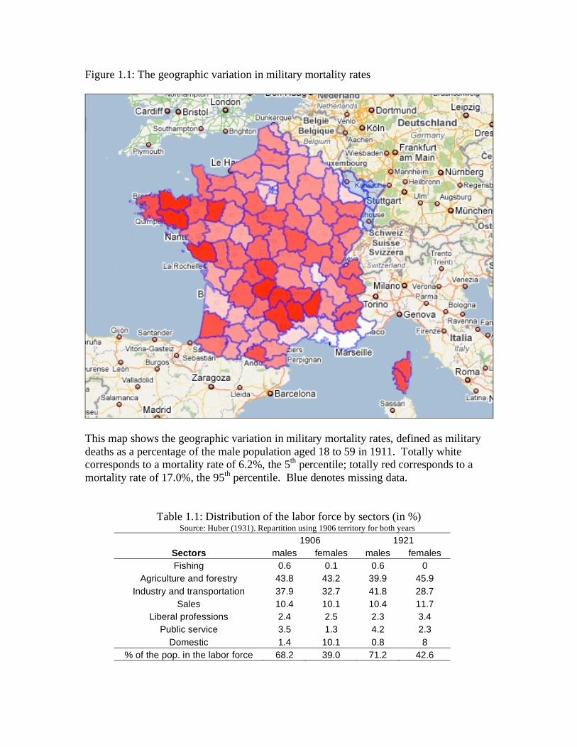
Figure 1.1: The geographic variation in military mortality rates

This map shows the geographic variation in military mortality rates, defined as military

deaths as a percentage of the male population aged 18 to 59 in 1911. Totally white

corresponds to a mortality rate of 6.2%, the 5th

percentile; totally red corresponds to a

mortality rate of 17.0%, the 95th percentile. Blue denotes missing data.

Table 1.1: Distribution of the labor force by sectors (in %) Source: Huber (1931). Repartition using 1906 territory for both years

1906 1921 Sectors males females males females Fishing 0.6 0.1 0.6 0

Agriculture and forestry 43.8 43.2 39.9 45.9 Industry and transportation 37.9 32.7 41.8 28.7

Sales 10.4 10.1 10.4 11.7 Liberal professions 2.4 2.5 2.3 3.4

Public service 3.5 1.3 4.2 2.3 Domestic 1.4 10.1 0.8 8

% of the pop. in the labor force 68.2 39.0 71.2 42.6

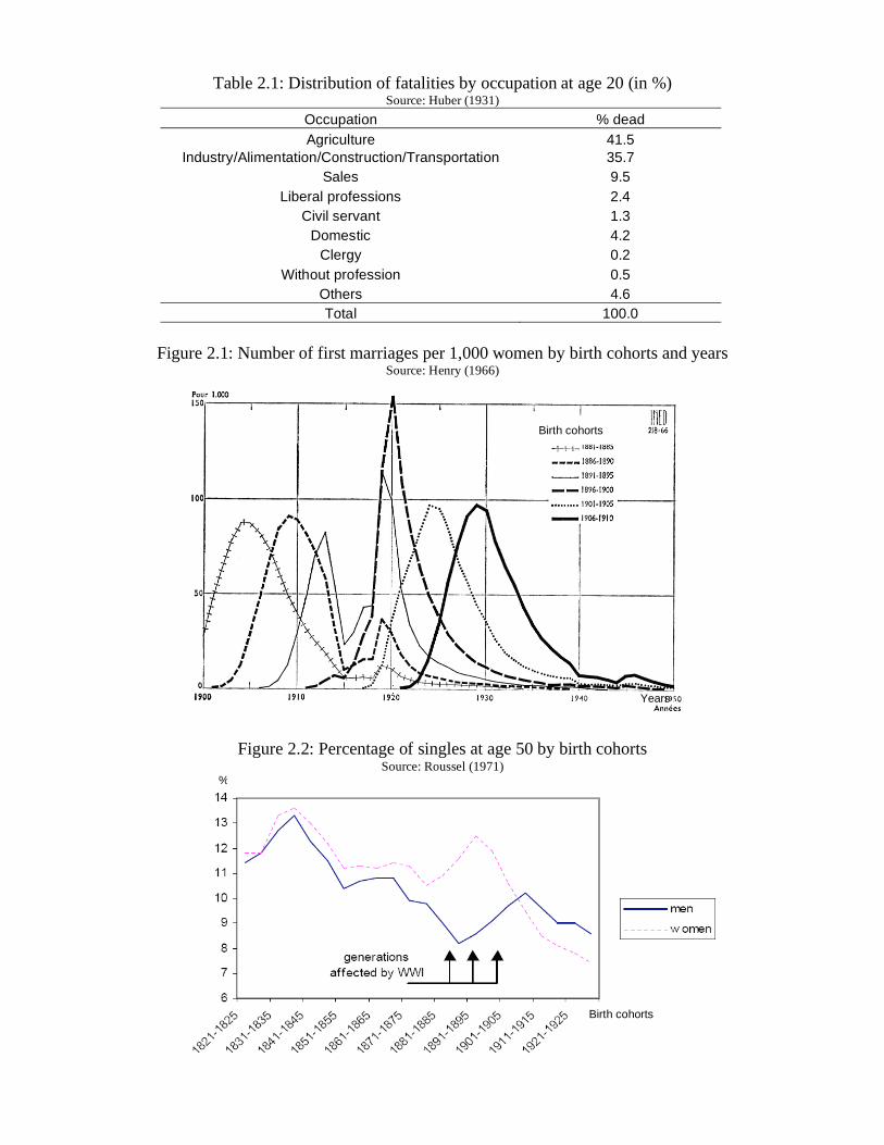
Table 2.1: Distribution of fatalities by occupation at age 20 (in %) Source: Huber (1931)

Occupation % dead Agriculture 41.5

Industry/Alimentation/Construction/Transportation 35.7 Sales 9.5

Liberal professions 2.4 Civil servant 1.3

Domestic 4.2 Clergy 0.2

Without profession 0.5 Others 4.6 Total 100.0

Figure 2.1: Number of first marriages per 1,000 women by birth cohorts and years Source: Henry (1966)

Figure 2.2: Percentage of singles at age 50 by birth cohorts Source: Roussel (1971)

Birth cohorts

Birth cohorts

Years

%

Table 2.2: Women were more likely to be unmarried in areas with higher mortality rates and lower sex ratios Dependent variable: fraction of women who aren't married (1) (2) (3) (4) (5) (6) (7) (8) Military Mortality 0.003*** 0.003*** 0.005*** 0.003*** (0.000) (0.000) (0.001) (0.000) Sex Ratio -0.300*** -0.295*** -0.255*** -0.028 (0.032) (0.023) (0.036) (0.026) Departement Dummies No Yes No Yes No Yes No Yes Census Period Dummies No No Yes Yes No No Yes Yes R-Squared 0.136 0.914 0.208 0.974 0.254 0.911 0.293 0.967 Observations 254 254 254 254 260 260 260 260 Notes: An observation is a departement in a census period (1911, 1921 or 1926). The sex ratio is defined as men aged 18-59 divided by women aged 15-49. Military mortality is the mortality rate of soldiers as a percentage of the male population aged 18 to 59 in 1911; it is set to zero for departements in the pre-war period. Unmarried women include women who have never been married, widowed women, and divorced women. Standard errors are given in parentheses. Asterisks indicate: * p<0.10, ** p<0.05, *** p<0.01.

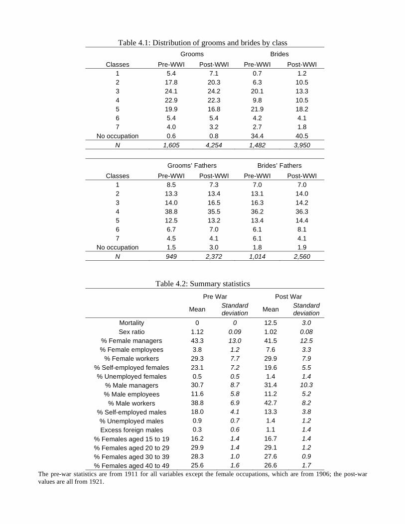
Table 4.1: Distribution of grooms and brides by class

Grooms Brides Classes Pre-WWI Post-WWI Pre-WWI Post-WWI

1 5.4 7.1 0.7 1.2 2 17.8 20.3 6.3 10.5 3 24.1 24.2 20.1 13.3 4 22.9 22.3 9.8 10.5 5 19.9 16.8 21.9 18.2 6 5.4 5.4 4.2 4.1 7 4.0 3.2 2.7 1.8

No occupation 0.6 0.8 34.4 40.5 N 1,605 4,254 1,482 3,950

Grooms’ Fathers Brides’ Fathers Classes Pre-WWI Post-WWI Pre-WWI Post-WWI

1 8.5 7.3 7.0 7.0 2 13.3 13.4 13.1 14.0 3 14.0 16.5 16.3 14.2 4 38.8 35.5 36.2 36.3 5 12.5 13.2 13.4 14.4 6 6.7 7.0 6.1 8.1 7 4.5 4.1 6.1 4.1

No occupation 1.5 3.0 1.8 1.9 N 949 2,372 1,014 2,560

Table 4.2: Summary statistics

Pre War Post War

Mean Standard

deviation Mean Standard

deviation

Mortality 0 0 12.5 3.0

Sex ratio 1.12 0.09 1.02 0.08

% Female managers 43.3 13.0 41.5 12.5

% Female employees 3.8 1.2 7.6 3.3

% Female workers 29.3 7.7 29.9 7.9

% Self-employed females 23.1 7.2 19.6 5.5

% Unemployed females 0.5 0.5 1.4 1.4

% Male managers 30.7 8.7 31.4 10.3

% Male employees 11.6 5.8 11.2 5.2

% Male workers 38.8 6.9 42.7 8.2

% Self-employed males 18.0 4.1 13.3 3.8

% Unemployed males 0.9 0.7 1.4 1.2

Excess foreign males 0.3 0.6 1.1 1.4

% Females aged 15 to 19 16.2 1.4 16.7 1.4

% Females aged 20 to 29 29.9 1.4 29.1 1.2

% Females aged 30 to 39 28.3 1.0 27.6 0.9

% Females aged 40 to 49 25.6 1.6 26.6 1.7

The pre-war statistics are from 1911 for all variables except the female occupations, which are from 1906; the post-war

values are all from 1921.

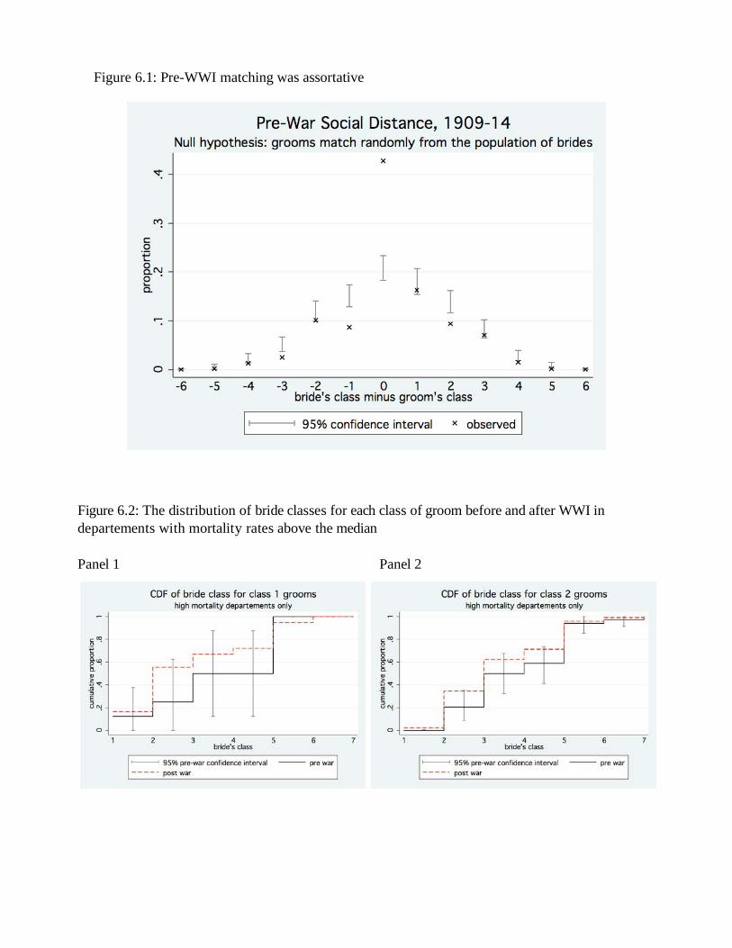
Figure 6.1: Pre-WWI matching was assortative

Figure 6.2: The distribution of bride classes for each class of groom before and after WWI in

departements with mortality rates above the median

Panel 1 Panel 2

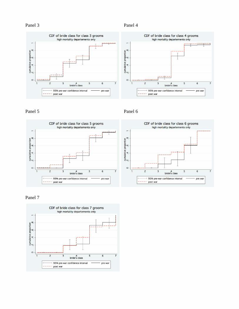
Panel 3 Panel 4

Panel 5 Panel 6

Panel 7

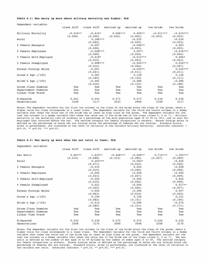
Table 6.1: Men marry up more where military mortality was higher, OLS Dependent variable: class diff class diff married up married up low bride low bride Military Mortality -0.016** -0.012* 0.006*** 0.005** -0.011*** -0.010*** (0.006) (0.006) (0.002) (0.002) (0.003) (0.003) Rural 0.186*** -0.032 -0.034 (0.064) (0.020) (0.022) % Female Managers -0.007 -0.006** 0.003 (0.008) (0.003) (0.003) % Female Employees -0.048*** 0.007* -0.016*** (0.009) (0.004) (0.004) % Female Self-Employed -0.018* -0.012*** 0.006* (0.010) (0.003) (0.003) % Female Unemployed 0.098*** -0.045*** 0.054*** (0.016) (0.006) (0.007) Excess Foreign Males -0.051 -0.025** 0.035*** (0.041) (0.011) (0.011) Groom's Age (/100) 0.381 0.158 0.156 (0.340) (0.124) (0.111) Bride's Age (/100) -0.581 -0.080 -0.086 (0.416) (0.133) (0.188) Groom Class Dummies Yes Yes Yes Yes Yes Yes Departement Dummies Yes Yes Yes Yes Yes Yes Linear Time Trend Yes Yes Yes Yes Yes Yes R-Squared 0.241 0.243 0.271 0.273 0.234 0.236 Observations 3158 3117 3033 2994 3158 3117 Notes: The dependent variable for the first two columns is the class of the bride minus the class of the groom, where a higher value for class corresponds to a lower class. The dependent variable for the third and fourth columns is a dummy variable that takes the value one if the bride was at least as high class as the groom. The dependent variable for the

last two columns is a dummy variable that takes the value one if the bride was of low class (class 5, 6 or 7). Military mortality is the mortality rate of soldiers as a percentage of the male population aged 18 to 59 in 1911, and is zero for marriages that occurred before the war. The omitted category for female occupations is workers. Excess foreign males is defined as the percentage of males who are foreign minus the percentage of females who are foreign. Standard errors, given in parentheses, are clustered at the level of variation in the variable military mortality. Asterisks indicate: *

p<0.10, ** p<0.05, *** p<0.01.

Table 6.2: Men marry up more when the sex ratio is lower, OLS Dependent variable: class diff class diff married up married up low bride low bride Sex Ratio 0.847** 1.633** -0.448*** -0.658** 0.714*** 1.302*** (0.410) (0.688) (0.153) (0.285) (0.207) (0.280) Rural 0.203*** -0.042* -0.026 (0.071) (0.024) (0.026) % Female Managers -0.015 0.002 -0.008 (0.015) (0.006) (0.006) % Female Employees -0.006 -0.004 -0.000 (0.023) (0.007) (0.009) % Female Self-Employed -0.002 -0.005 0.002 (0.019) (0.006) (0.008) % Female Unemployed 0.021 -0.004 0.017** (0.020) (0.006) (0.007) Excess Foreign Males 0.002 -0.006 0.007 (0.063) (0.016) (0.020) Groom's Age (/100) 0.194 0.194 0.101 (0.482) (0.151) (0.180) Bride's Age (/100) -0.514 -0.096 -0.074 (0.480) (0.151) (0.171) Groom Class Dummies Yes Yes Yes Yes Yes Yes Departement Dummies Yes Yes Yes Yes Yes Yes Linear Time Trend Yes Yes Yes Yes Yes Yes R-Squared 0.232 0.239 0.270 0.272 0.226 0.232 Observations 3208 3175 3080 3048 3208 3175 Notes: The dependent variable for the first two columns is the class of the bride minus the class of the groom, where a higher value for class corresponds to a lower class. The dependent variable for the third and fourth columns is a dummy

variable that takes the value one if the bride was at least as high class as the groom. The dependent variable for the last two columns is a dummy variable that takes the value one if the bride was of low class (class 5, 6 or 7). The sex ratio is defined as the number of men aged 18 to 59 divided by the number of women aged 15 to 49. The omitted category for female occupations is workers. Excess foreign males is defined as the percentage of males who are foreign minus the percentage of females who are foreign. Standard errors, given in parentheses, are clustered at the level of variation in

the variable sex ratio. Asterisks indicate: * p<0.10, ** p<0.05, *** p<0.01.

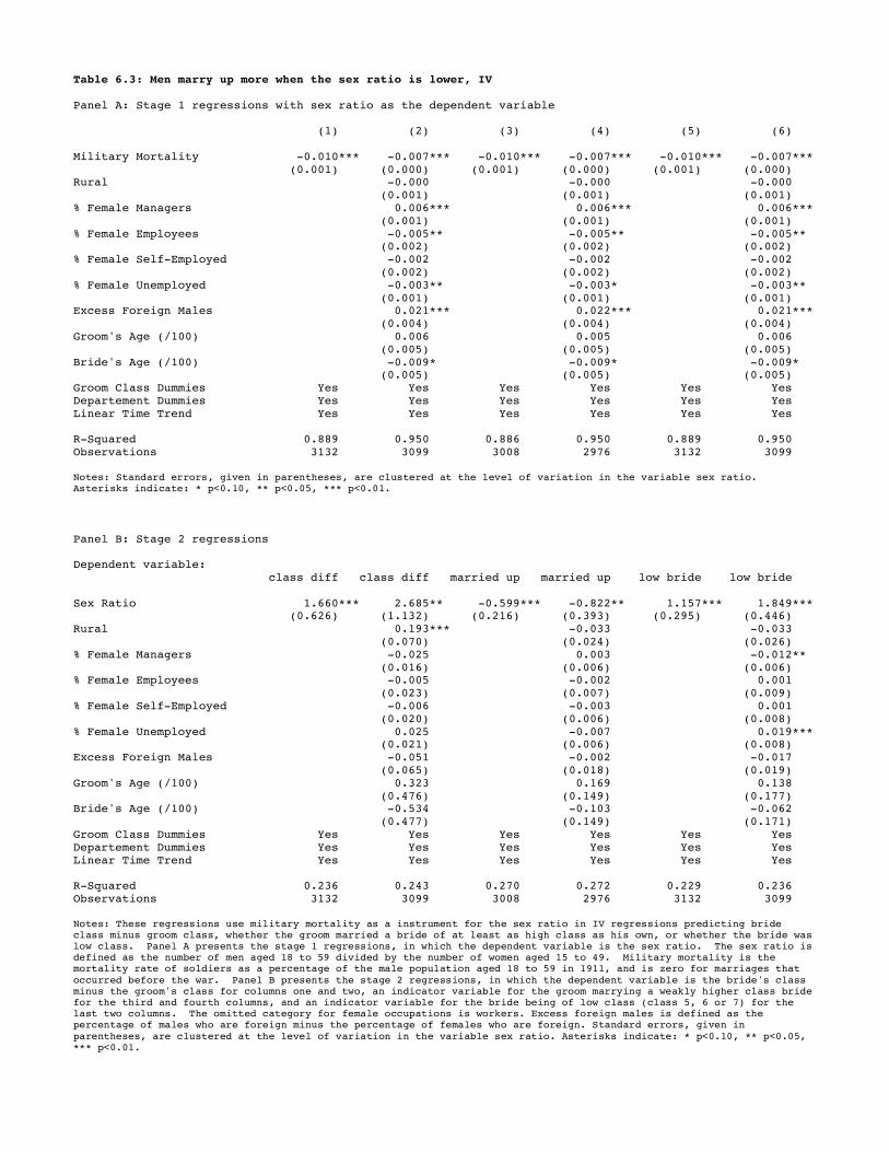
Table 6.3: Men marry up more when the sex ratio is lower, IV Panel A: Stage 1 regressions with sex ratio as the dependent variable (1) (2) (3) (4) (5) (6) Military Mortality -0.010*** -0.007*** -0.010*** -0.007*** -0.010*** -0.007*** (0.001) (0.000) (0.001) (0.000) (0.001) (0.000) Rural -0.000 -0.000 -0.000 (0.001) (0.001) (0.001) % Female Managers 0.006*** 0.006*** 0.006*** (0.001) (0.001) (0.001) % Female Employees -0.005** -0.005** -0.005** (0.002) (0.002) (0.002) % Female Self-Employed -0.002 -0.002 -0.002 (0.002) (0.002) (0.002) % Female Unemployed -0.003** -0.003* -0.003** (0.001) (0.001) (0.001) Excess Foreign Males 0.021*** 0.022*** 0.021*** (0.004) (0.004) (0.004) Groom's Age (/100) 0.006 0.005 0.006 (0.005) (0.005) (0.005) Bride's Age (/100) -0.009* -0.009* -0.009* (0.005) (0.005) (0.005) Groom Class Dummies Yes Yes Yes Yes Yes Yes Departement Dummies Yes Yes Yes Yes Yes Yes Linear Time Trend Yes Yes Yes Yes Yes Yes R-Squared 0.889 0.950 0.886 0.950 0.889 0.950 Observations 3132 3099 3008 2976 3132 3099 Notes: Standard errors, given in parentheses, are clustered at the level of variation in the variable sex ratio. Asterisks indicate: * p<0.10, ** p<0.05, *** p<0.01.

Panel B: Stage 2 regressions Dependent variable: class diff class diff married up married up low bride low bride Sex Ratio 1.660*** 2.685** -0.599*** -0.822** 1.157*** 1.849*** (0.626) (1.132) (0.216) (0.393) (0.295) (0.446) Rural 0.193*** -0.033 -0.033 (0.070) (0.024) (0.026) % Female Managers -0.025 0.003 -0.012** (0.016) (0.006) (0.006) % Female Employees -0.005 -0.002 0.001 (0.023) (0.007) (0.009) % Female Self-Employed -0.006 -0.003 0.001 (0.020) (0.006) (0.008) % Female Unemployed 0.025 -0.007 0.019*** (0.021) (0.006) (0.008) Excess Foreign Males -0.051 -0.002 -0.017 (0.065) (0.018) (0.019) Groom's Age (/100) 0.323 0.169 0.138 (0.476) (0.149) (0.177) Bride's Age (/100) -0.534 -0.103 -0.062 (0.477) (0.149) (0.171) Groom Class Dummies Yes Yes Yes Yes Yes Yes Departement Dummies Yes Yes Yes Yes Yes Yes Linear Time Trend Yes Yes Yes Yes Yes Yes R-Squared 0.236 0.243 0.270 0.272 0.229 0.236 Observations 3132 3099 3008 2976 3132 3099 Notes: These regressions use military mortality as a instrument for the sex ratio in IV regressions predicting bride class minus groom class, whether the groom married a bride of at least as high class as his own, or whether the bride was low class. Panel A presents the stage 1 regressions, in which the dependent variable is the sex ratio. The sex ratio is defined as the number of men aged 18 to 59 divided by the number of women aged 15 to 49. Military mortality is the mortality rate of soldiers as a percentage of the male population aged 18 to 59 in 1911, and is zero for marriages that

occurred before the war. Panel B presents the stage 2 regressions, in which the dependent variable is the bride's class minus the groom's class for columns one and two, an indicator variable for the groom marrying a weakly higher class bride for the third and fourth columns, and an indicator variable for the bride being of low class (class 5, 6 or 7) for the last two columns. The omitted category for female occupations is workers. Excess foreign males is defined as the percentage of males who are foreign minus the percentage of females who are foreign. Standard errors, given in

parentheses, are clustered at the level of variation in the variable sex ratio. Asterisks indicate: * p<0.10, ** p<0.05, *** p<0.01.

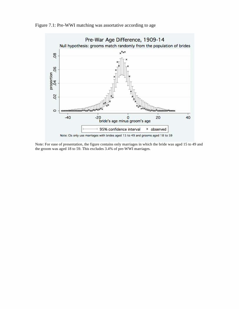
Figure 7.1: Pre-WWI matching was assortative according to age

Note: For ease of presentation, the figure contains only marriages in which the bride was aged 15 to 49 and

the groom was aged 18 to 59. This excludes 3.4% of pre-WWI marriages.

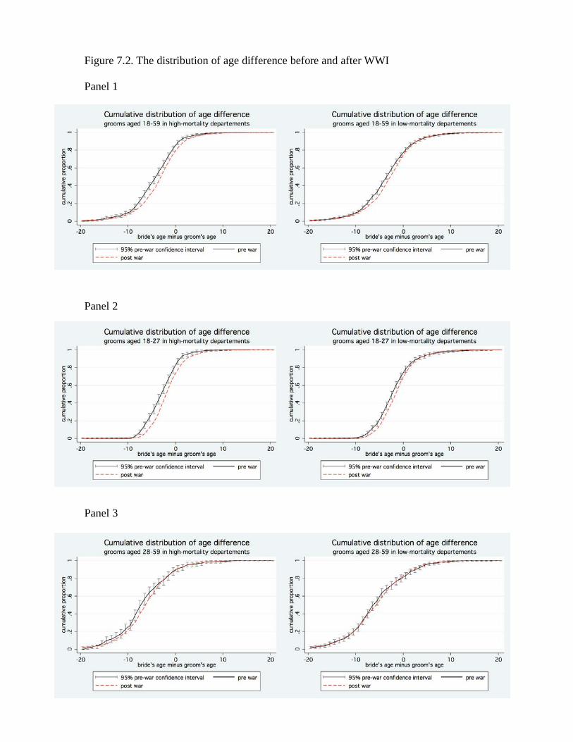
Figure 7.2. The distribution of age difference before and after WWI

Panel 1

Panel 2

Panel 3

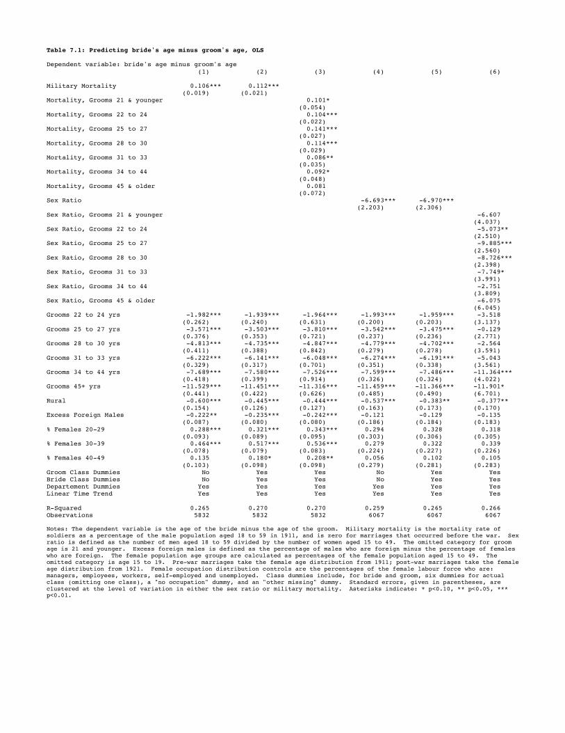
Table 7.1: Predicting bride's age minus groom's age, OLS Dependent variable: bride's age minus groom's age

(1) (2) (3) (4) (5) (6) Military Mortality 0.106*** 0.112*** (0.019) (0.021) Mortality, Grooms 21 & younger 0.101*

(0.054) Mortality, Grooms 22 to 24 0.104*** (0.022) Mortality, Grooms 25 to 27 0.141*** (0.027)

Mortality, Grooms 28 to 30 0.114*** (0.029) Mortality, Grooms 31 to 33 0.086** (0.035) Mortality, Grooms 34 to 44 0.092*

(0.048) Mortality, Grooms 45 & older 0.081 (0.072) Sex Ratio -6.693*** -6.970*** (2.203) (2.306)

Sex Ratio, Grooms 21 & younger -6.607 (4.037) Sex Ratio, Grooms 22 to 24 -5.073** (2.510) Sex Ratio, Grooms 25 to 27 -9.885***

(2.560) Sex Ratio, Grooms 28 to 30 -8.726*** (2.398) Sex Ratio, Grooms 31 to 33 -7.749* (3.991)

Sex Ratio, Grooms 34 to 44 -2.751 (3.809) Sex Ratio, Grooms 45 & older -6.075 (6.045) Grooms 22 to 24 yrs -1.982*** -1.939*** -1.964*** -1.993*** -1.959*** -3.518

(0.262) (0.240) (0.631) (0.200) (0.203) (3.137) Grooms 25 to 27 yrs -3.571*** -3.503*** -3.810*** -3.542*** -3.475*** -0.129 (0.376) (0.353) (0.721) (0.237) (0.236) (2.771) Grooms 28 to 30 yrs -4.813*** -4.735*** -4.847*** -4.779*** -4.702*** -2.564 (0.411) (0.388) (0.842) (0.279) (0.278) (3.591)

Grooms 31 to 33 yrs -6.222*** -6.141*** -6.048*** -6.274*** -6.191*** -5.043 (0.329) (0.317) (0.701) (0.351) (0.338) (3.561) Grooms 34 to 44 yrs -7.689*** -7.580*** -7.526*** -7.599*** -7.486*** -11.364*** (0.418) (0.399) (0.914) (0.326) (0.324) (4.022) Grooms 45+ yrs -11.529*** -11.451*** -11.316*** -11.459*** -11.366*** -11.901*

(0.441) (0.422) (0.626) (0.485) (0.490) (6.701) Rural -0.600*** -0.445*** -0.444*** -0.537*** -0.383** -0.377** (0.154) (0.126) (0.127) (0.163) (0.173) (0.170) Excess Foreign Males -0.222** -0.235*** -0.242*** -0.121 -0.129 -0.135 (0.087) (0.080) (0.080) (0.186) (0.184) (0.183)

% Females 20-29 0.288*** 0.321*** 0.343*** 0.294 0.328 0.318 (0.093) (0.089) (0.095) (0.303) (0.306) (0.305) % Females 30-39 0.464*** 0.517*** 0.536*** 0.279 0.322 0.339 (0.078) (0.079) (0.083) (0.224) (0.227) (0.226) % Females 40-49 0.135 0.180* 0.208** 0.056 0.102 0.105

(0.103) (0.098) (0.098) (0.279) (0.281) (0.283) Groom Class Dummies No Yes Yes No Yes Yes Bride Class Dummies No Yes Yes No Yes Yes Departement Dummies Yes Yes Yes Yes Yes Yes Linear Time Trend Yes Yes Yes Yes Yes Yes

R-Squared 0.265 0.270 0.270 0.259 0.265 0.266 Observations 5832 5832 5832 6067 6067 6067 Notes: The dependent variable is the age of the bride minus the age of the groom. Military mortality is the mortality rate of soldiers as a percentage of the male population aged 18 to 59 in 1911, and is zero for marriages that occurred before the war. Sex ratio is defined as the number of men aged 18 to 59 divided by the number of women aged 15 to 49. The omitted category for groom age is 21 and younger. Excess foreign males is defined as the percentage of males who are foreign minus the percentage of females who are foreign. The female population age groups are calculated as percentages of the female population aged 15 to 49. The omitted category is age 15 to 19. Pre-war marriages take the female age distribution from 1911; post-war marriages take the female age distribution from 1921. Female occupation distribution controls are the percentages of the female labour force who are: managers, employees, workers, self-employed and unemployed. Class dummies include, for bride and groom, six dummies for actual class (omitting one class), a "no occupation" dummy, and an "other missing" dummy. Standard errors, given in parentheses, are clustered at the level of variation in either the sex ratio or military mortality. Asterisks indicate: * p<0.10, ** p<0.05, *** p<0.01.

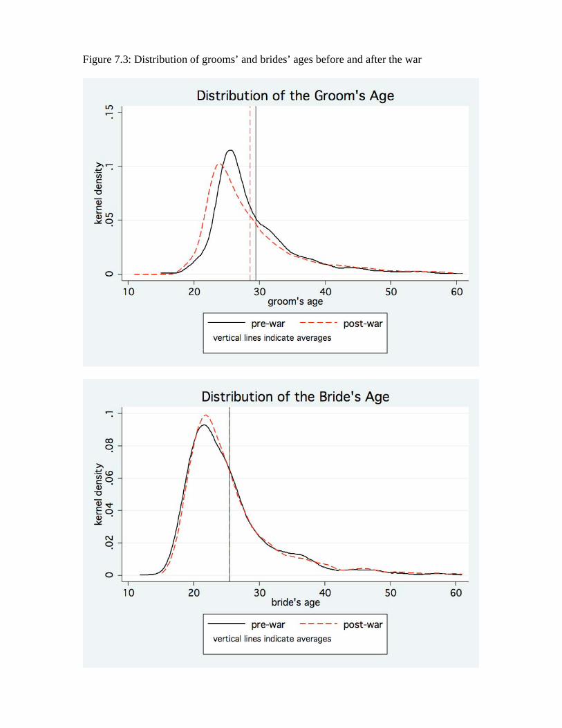
Figure 7.3: Distribution of grooms’ and brides’ ages before and after the war

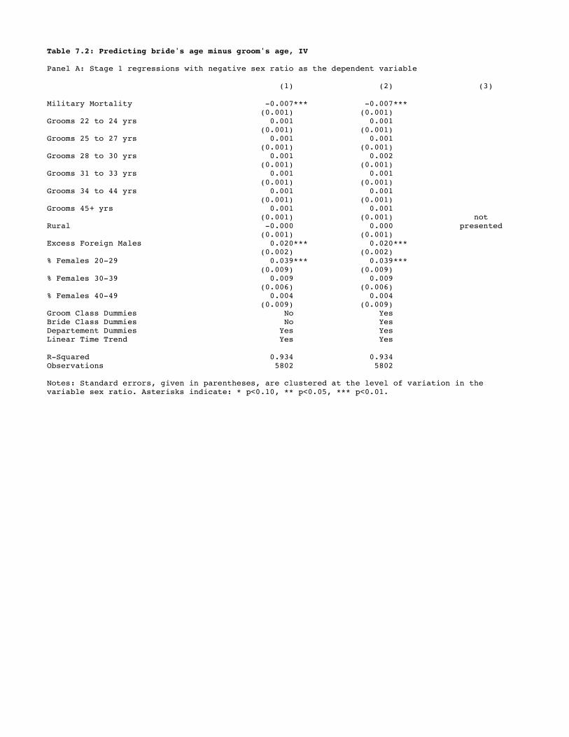
Table 7.2: Predicting bride's age minus groom's age, IV Panel A: Stage 1 regressions with negative sex ratio as the dependent variable (1) (2) (3)

Military Mortality -0.007*** -0.007*** (0.001) (0.001) Grooms 22 to 24 yrs 0.001 0.001 (0.001) (0.001) Grooms 25 to 27 yrs 0.001 0.001 (0.001) (0.001) Grooms 28 to 30 yrs 0.001 0.002 (0.001) (0.001) Grooms 31 to 33 yrs 0.001 0.001

(0.001) (0.001) Grooms 34 to 44 yrs 0.001 0.001 (0.001) (0.001) Grooms 45+ yrs 0.001 0.001 (0.001) (0.001) not Rural -0.000 0.000 presented (0.001) (0.001) Excess Foreign Males 0.020*** 0.020*** (0.002) (0.002) % Females 20-29 0.039*** 0.039***

(0.009) (0.009) % Females 30-39 0.009 0.009 (0.006) (0.006) % Females 40-49 0.004 0.004 (0.009) (0.009) Groom Class Dummies No Yes Bride Class Dummies No Yes Departement Dummies Yes Yes Linear Time Trend Yes Yes

R-Squared 0.934 0.934 Observations 5802 5802 Notes: Standard errors, given in parentheses, are clustered at the level of variation in the variable sex ratio. Asterisks indicate: * p<0.10, ** p<0.05, *** p<0.01.

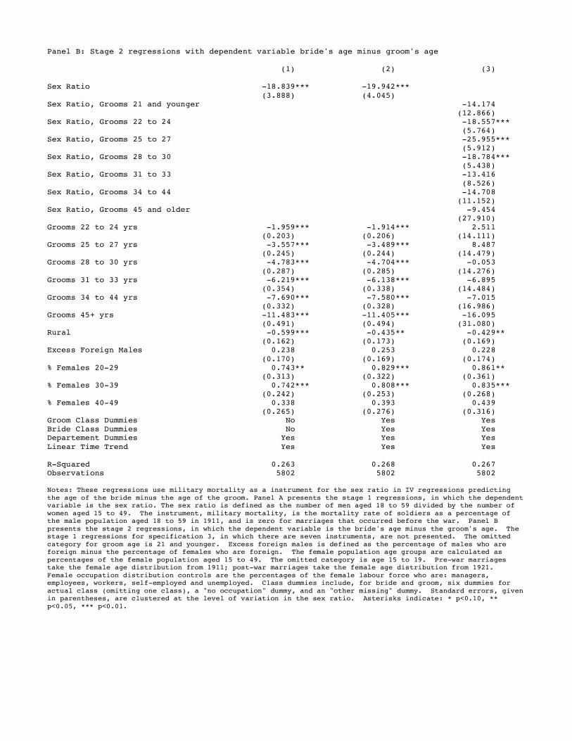
Panel B: Stage 2 regressions with dependent variable bride's age minus groom's age (1) (2) (3) Sex Ratio -18.839*** -19.942***

(3.888) (4.045) Sex Ratio, Grooms 21 and younger -14.174 (12.866) Sex Ratio, Grooms 22 to 24 -18.557*** (5.764) Sex Ratio, Grooms 25 to 27 -25.955*** (5.912) Sex Ratio, Grooms 28 to 30 -18.784*** (5.438) Sex Ratio, Grooms 31 to 33 -13.416

(8.526) Sex Ratio, Grooms 34 to 44 -14.708 (11.152) Sex Ratio, Grooms 45 and older -9.454 (27.910) Grooms 22 to 24 yrs -1.959*** -1.914*** 2.511 (0.203) (0.206) (14.111) Grooms 25 to 27 yrs -3.557*** -3.489*** 8.487 (0.245) (0.244) (14.479) Grooms 28 to 30 yrs -4.783*** -4.704*** -0.053

(0.287) (0.285) (14.276) Grooms 31 to 33 yrs -6.219*** -6.138*** -6.895 (0.354) (0.338) (14.484) Grooms 34 to 44 yrs -7.690*** -7.580*** -7.015 (0.332) (0.328) (16.986) Grooms 45+ yrs -11.483*** -11.405*** -16.095 (0.491) (0.494) (31.080) Rural -0.599*** -0.435** -0.429** (0.162) (0.173) (0.169) Excess Foreign Males 0.238 0.253 0.228

(0.170) (0.169) (0.174) % Females 20-29 0.743** 0.829*** 0.861** (0.313) (0.322) (0.361) % Females 30-39 0.742*** 0.808*** 0.835*** (0.242) (0.253) (0.268) % Females 40-49 0.338 0.393 0.439 (0.265) (0.276) (0.316) Groom Class Dummies No Yes Yes Bride Class Dummies No Yes Yes Departement Dummies Yes Yes Yes

Linear Time Trend Yes Yes Yes R-Squared 0.263 0.268 0.267 Observations 5802 5802 5802 Notes: These regressions use military mortality as a instrument for the sex ratio in IV regressions predicting

the age of the bride minus the age of the groom. Panel A presents the stage 1 regressions, in which the dependent variable is the sex ratio. The sex ratio is defined as the number of men aged 18 to 59 divided by the number of

women aged 15 to 49. The instrument, military mortality, is the mortality rate of soldiers as a percentage of the male population aged 18 to 59 in 1911, and is zero for marriages that occurred before the war. Panel B

presents the stage 2 regressions, in which the dependent variable is the bride's age minus the groom's age. The stage 1 regressions for specification 3, in which there are seven instruments, are not presented. The omitted

category for groom age is 21 and younger. Excess foreign males is defined as the percentage of males who are foreign minus the percentage of females who are foreign. The female population age groups are calculated as

percentages of the female population aged 15 to 49. The omitted category is age 15 to 19. Pre-war marriages take the female age distribution from 1911; post-war marriages take the female age distribution from 1921.

Female occupation distribution controls are the percentages of the female labour force who are: managers, employees, workers, self-employed and unemployed. Class dummies include, for bride and groom, six dummies for

actual class (omitting one class), a "no occupation" dummy, and an "other missing" dummy. Standard errors, given in parentheses, are clustered at the level of variation in the sex ratio. Asterisks indicate: * p<0.10, **

p<0.05, *** p<0.01.

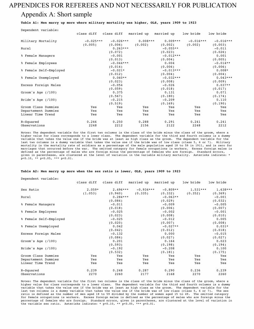
Table A1: Men marry up more where military mortality was higher, OLS, years 1909 to 1923 Dependent variable: class diff class diff married up married up low bride low bride Military Mortality -0.025*** -0.026*** 0.008*** 0.009*** -0.016*** -0.016*** (0.005) (0.006) (0.002) (0.002) (0.002) (0.003) Rural 0.263*** -0.055** -0.011 (0.072) (0.023) (0.026) % Female Managers -0.001 -0.012*** 0.001 (0.013) (0.004) (0.005) % Female Employees -0.044*** 0.004 -0.014** (0.014) (0.006) (0.006) % Female Self-Employed -0.021* -0.013*** 0.008* (0.012) (0.004) (0.004) % Female Unemployed 0.060** -0.032*** 0.043*** (0.023) (0.008) (0.009) Excess Foreign Males -0.054 -0.026 0.037** (0.059) (0.018) (0.017) Groom's Age (/100) 0.375 0.131 0.071 (0.567) (0.180) (0.174) Bride's Age (/100) -0.215 -0.209 0.110 (0.519) (0.169) (0.190) Groom Class Dummies Yes Yes Yes Yes Yes Yes Departement Dummies Yes Yes Yes Yes Yes Yes Linear Time Trend Yes Yes Yes Yes Yes Yes R-Squared 0.246 0.250 0.288 0.291 0.241 0.241 Observations 2248 2212 2156 2122 2248 2212 Notes: The dependent variable for the first two columns is the class of the bride minus the class of the groom, where a higher value for class corresponds to a lower class. The dependent variable for the third and fourth columns is a dummy variable that takes the value one if the bride was at least as high class as the groom. The dependent variable for the

last two columns is a dummy variable that takes the value one if the bride was of low class (class 5, 6 or 7). Military mortality is the mortality rate of soldiers as a percentage of the male population aged 18 to 59 in 1911, and is zero for marriages that occurred before the war. The omitted category for female occupations is workers. Excess foreign males is defined as the percentage of males who are foreign minus the percentage of females who are foreign. Standard errors, given in parentheses, are clustered at the level of variation in the variable military mortality. Asterisks indicate: *

p<0.10, ** p<0.05, *** p<0.01.

Table A2: Men marry up more when the sex ratio is lower, OLS, years 1909 to 1923 Dependent variable: class diff class diff married up married up low bride low bride Sex Ratio 2.059* 2.496*** -0.934*** -0.809** 1.531*** 1.638*** (1.053) (0.940) (0.335) (0.332) (0.352) (0.369) Rural 0.284*** -0.063** -0.001 (0.084) (0.029) (0.032) % Female Managers -0.011 -0.009 -0.005 (0.018) (0.006) (0.007) % Female Employees -0.025 -0.002 -0.001 (0.023) (0.008) (0.010) % Female Self-Employed -0.025 -0.012 0.005 (0.020) (0.007) (0.008) % Female Unemployed 0.042 -0.027** 0.031* (0.042) (0.012) (0.018) Excess Foreign Males -0.132 0.000 -0.015 (0.084) (0.027) (0.027) Groom's Age (/100) 0.201 0.164 0.023 (0.593) (0.198) (0.194) Bride's Age (/100) -0.192 -0.208 0.100 (0.532) (0.181) (0.175) Groom Class Dummies Yes Yes Yes Yes Yes Yes Departement Dummies Yes Yes Yes Yes Yes Yes Linear Time Trend Yes Yes Yes Yes Yes Yes R-Squared 0.239 0.248 0.287 0.290 0.236 0.239 Observations 2270 2260 2177 2168 2270 2260 Notes: The dependent variable for the first two columns is the class of the bride minus the class of the groom, where a

higher value for class corresponds to a lower class. The dependent variable for the third and fourth columns is a dummy variable that takes the value one if the bride was at least as high class as the groom. The dependent variable for the last two columns is a dummy variable that takes the value one if the bride was of low class (class 5, 6 or 7). The sex ratio is defined as the number of men aged 18 to 59 divided by the number of women aged 15 to 49. The omitted category for female occupations is workers. Excess foreign males is defined as the percentage of males who are foreign minus the

percentage of females who are foreign. Standard errors, given in parentheses, are clustered at the level of variation in the variable sex ratio. Asterisks indicate: * p<0.10, ** p<0.05, *** p<0.01.

Appendix A: Short sampleAPPENDICES FOR REFEREES AND NOT NECESSARILY FOR PUBLICATION

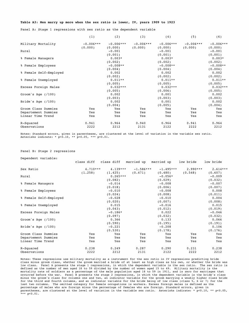
Table A3: Men marry up more when the sex ratio is lower, IV, years 1909 to 1923 Panel A: Stage 1 regressions with sex ratio as the dependent variable (1) (2) (3) (4) (5) (6) Military Mortality -0.006*** -0.006*** -0.006*** -0.006*** -0.006*** -0.006*** (0.000) (0.000) (0.000) (0.000) (0.000) (0.000) Rural -0.001 -0.001 -0.001 (0.001) (0.001) (0.001) % Female Managers 0.003* 0.003* 0.003* (0.002) (0.002) (0.002) % Female Employees -0.008** -0.008** -0.008** (0.004) (0.004) (0.004) % Female Self-Employed 0.002 0.002 0.002 (0.002) (0.002) (0.002) % Female Unemployed 0.011** 0.011** 0.011** (0.005) (0.005) (0.005) Excess Foreign Males 0.032*** 0.032*** 0.032*** (0.005) (0.006) (0.005) Groom's Age (/100) 0.002 0.001 0.002 (0.003) (0.003) (0.003) Bride's Age (/100) 0.002 0.001 0.002 (0.004) (0.005) (0.004) Groom Class Dummies Yes Yes Yes Yes Yes Yes Departement Dummies Yes Yes Yes Yes Yes Yes Linear Time Trend Yes Yes Yes Yes Yes Yes R-Squared 0.941 0.964 0.940 0.964 0.941 0.964 Observations 2222 2212 2131 2122 2222 2212 Notes: Standard errors, given in parentheses, are clustered at the level of variation in the variable sex ratio. Asterisks indicate: * p<0.10, ** p<0.05, *** p<0.01.

Panel B: Stage 2 regressions Dependent variable: class diff class diff married up married up low bride low bride Sex Ratio 4.710*** 4.139*** -1.586*** -1.495*** 2.990*** 2.614*** (1.258) (1.425) (0.471) (0.480) (0.548) (0.607) Rural 0.265*** -0.056* -0.009 (0.082) (0.029) (0.032) % Female Managers -0.014 -0.008 -0.007 (0.018) (0.006) (0.007) % Female Employees -0.010 -0.008 0.008 (0.024) (0.008) (0.011) % Female Self-Employed -0.028 -0.010 0.004 (0.020) (0.007) (0.008) % Female Unemployed 0.015 -0.016 0.015 (0.043) (0.012) (0.019) Excess Foreign Males -0.186* 0.022 -0.046 (0.097) (0.032) (0.032) Groom's Age (/100) 0.366 0.133 0.066 (0.590) (0.195) (0.191) Bride's Age (/100) -0.221 -0.208 0.106 (0.530) (0.178) (0.176) Groom Class Dummies Yes Yes Yes Yes Yes Yes Departement Dummies Yes Yes Yes Yes Yes Yes Linear Time Trend Yes Yes Yes Yes Yes Yes R-Squared 0.238 0.249 0.287 0.290 0.231 0.238 Observations 2222 2212 2131 2122 2222 2212 Notes: These regressions use military mortality as a instrument for the sex ratio in IV regressions predicting bride class minus groom class, whether the groom married a bride of at least as high class as his own, or whether the bride was low class. Panel A presents the stage 1 regressions, in which the dependent variable is the sex ratio. The sex ratio is defined as the number of men aged 18 to 59 divided by the number of women aged 15 to 49. Military mortality is the mortality rate of soldiers as a percentage of the male population aged 18 to 59 in 1911, and is zero for marriages that

occurred before the war. Panel B presents the stage 2 regressions, in which the dependent variable is the bride's class minus the groom's class for columns one and two, an indicator variable for the groom marrying a weakly higher class bride for the third and fourth columns, and an indicator variable for the bride being of low class (class 5, 6 or 7) for the last two columns. The omitted category for female occupations is workers. Excess foreign males is defined as the percentage of males who are foreign minus the percentage of females who are foreign. Standard errors, given in

parentheses, are clustered at the level of variation in the variable sex ratio. Asterisks indicate: * p<0.10, ** p<0.05, *** p<0.01.

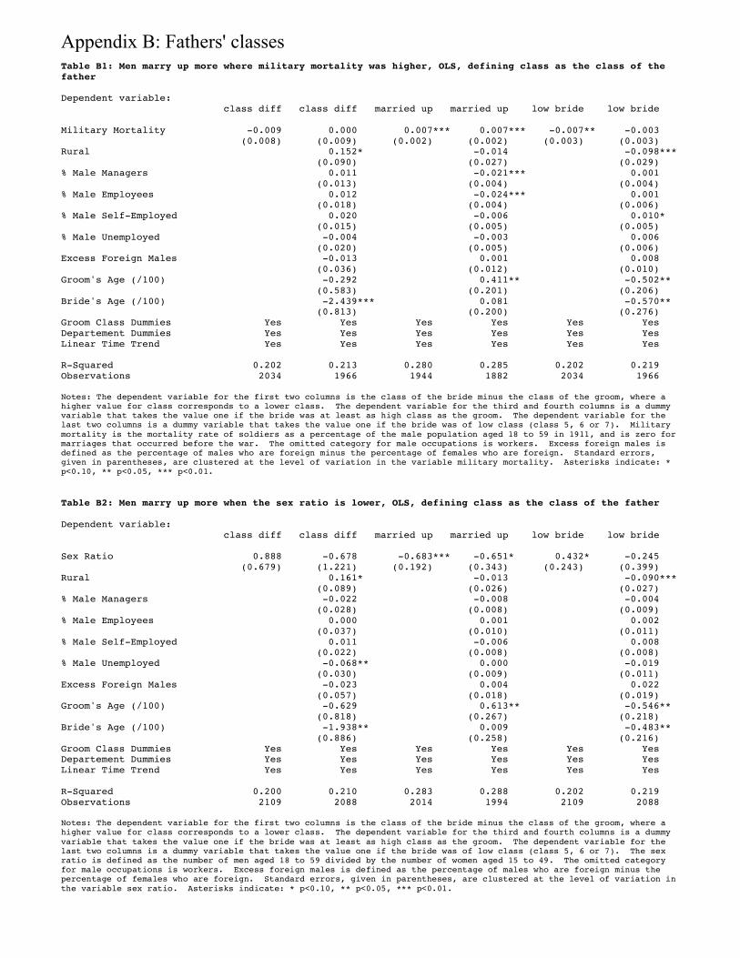
Table B1: Men marry up more where military mortality was higher, OLS, defining class as the class of the father Dependent variable: class diff class diff married up married up low bride low bride Military Mortality -0.009 0.000 0.007*** 0.007*** -0.007** -0.003 (0.008) (0.009) (0.002) (0.002) (0.003) (0.003) Rural 0.152* -0.014 -0.098*** (0.090) (0.027) (0.029) % Male Managers 0.011 -0.021*** 0.001 (0.013) (0.004) (0.004) % Male Employees 0.012 -0.024*** 0.001 (0.018) (0.004) (0.006) % Male Self-Employed 0.020 -0.006 0.010* (0.015) (0.005) (0.005) % Male Unemployed -0.004 -0.003 0.006 (0.020) (0.005) (0.006) Excess Foreign Males -0.013 0.001 0.008 (0.036) (0.012) (0.010) Groom's Age (/100) -0.292 0.411** -0.502** (0.583) (0.201) (0.206) Bride's Age (/100) -2.439*** 0.081 -0.570** (0.813) (0.200) (0.276) Groom Class Dummies Yes Yes Yes Yes Yes Yes Departement Dummies Yes Yes Yes Yes Yes Yes Linear Time Trend Yes Yes Yes Yes Yes Yes R-Squared 0.202 0.213 0.280 0.285 0.202 0.219 Observations 2034 1966 1944 1882 2034 1966 Notes: The dependent variable for the first two columns is the class of the bride minus the class of the groom, where a higher value for class corresponds to a lower class. The dependent variable for the third and fourth columns is a dummy variable that takes the value one if the bride was at least as high class as the groom. The dependent variable for the last two columns is a dummy variable that takes the value one if the bride was of low class (class 5, 6 or 7). Military

mortality is the mortality rate of soldiers as a percentage of the male population aged 18 to 59 in 1911, and is zero for marriages that occurred before the war. The omitted category for male occupations is workers. Excess foreign males is defined as the percentage of males who are foreign minus the percentage of females who are foreign. Standard errors, given in parentheses, are clustered at the level of variation in the variable military mortality. Asterisks indicate: * p<0.10, ** p<0.05, *** p<0.01.

Table B2: Men marry up more when the sex ratio is lower, OLS, defining class as the class of the father Dependent variable: class diff class diff married up married up low bride low bride Sex Ratio 0.888 -0.678 -0.683*** -0.651* 0.432* -0.245 (0.679) (1.221) (0.192) (0.343) (0.243) (0.399) Rural 0.161* -0.013 -0.090*** (0.089) (0.026) (0.027) % Male Managers -0.022 -0.008 -0.004 (0.028) (0.008) (0.009) % Male Employees 0.000 0.001 0.002 (0.037) (0.010) (0.011) % Male Self-Employed 0.011 -0.006 0.008 (0.022) (0.008) (0.008) % Male Unemployed -0.068** 0.000 -0.019 (0.030) (0.009) (0.011) Excess Foreign Males -0.023 0.004 0.022 (0.057) (0.018) (0.019) Groom's Age (/100) -0.629 0.613** -0.546** (0.818) (0.267) (0.218) Bride's Age (/100) -1.938** 0.009 -0.483** (0.886) (0.258) (0.216) Groom Class Dummies Yes Yes Yes Yes Yes Yes Departement Dummies Yes Yes Yes Yes Yes Yes Linear Time Trend Yes Yes Yes Yes Yes Yes R-Squared 0.200 0.210 0.283 0.288 0.202 0.219 Observations 2109 2088 2014 1994 2109 2088 Notes: The dependent variable for the first two columns is the class of the bride minus the class of the groom, where a higher value for class corresponds to a lower class. The dependent variable for the third and fourth columns is a dummy

variable that takes the value one if the bride was at least as high class as the groom. The dependent variable for the last two columns is a dummy variable that takes the value one if the bride was of low class (class 5, 6 or 7). The sex ratio is defined as the number of men aged 18 to 59 divided by the number of women aged 15 to 49. The omitted category for male occupations is workers. Excess foreign males is defined as the percentage of males who are foreign minus the percentage of females who are foreign. Standard errors, given in parentheses, are clustered at the level of variation in

the variable sex ratio. Asterisks indicate: * p<0.10, ** p<0.05, *** p<0.01.

Appendix B: Fathers' classes

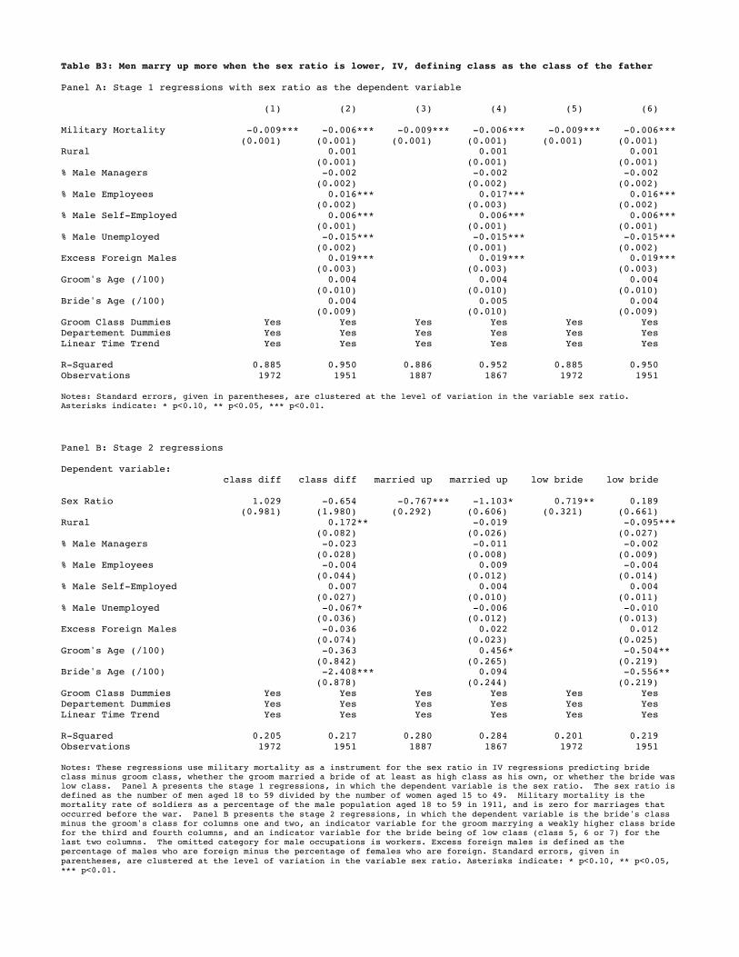
Table B3: Men marry up more when the sex ratio is lower, IV, defining class as the class of the father Panel A: Stage 1 regressions with sex ratio as the dependent variable (1) (2) (3) (4) (5) (6) Military Mortality -0.009*** -0.006*** -0.009*** -0.006*** -0.009*** -0.006*** (0.001) (0.001) (0.001) (0.001) (0.001) (0.001) Rural 0.001 0.001 0.001 (0.001) (0.001) (0.001) % Male Managers -0.002 -0.002 -0.002 (0.002) (0.002) (0.002) % Male Employees 0.016*** 0.017*** 0.016*** (0.002) (0.003) (0.002) % Male Self-Employed 0.006*** 0.006*** 0.006*** (0.001) (0.001) (0.001) % Male Unemployed -0.015*** -0.015*** -0.015*** (0.002) (0.001) (0.002) Excess Foreign Males 0.019*** 0.019*** 0.019*** (0.003) (0.003) (0.003) Groom's Age (/100) 0.004 0.004 0.004 (0.010) (0.010) (0.010) Bride's Age (/100) 0.004 0.005 0.004 (0.009) (0.010) (0.009) Groom Class Dummies Yes Yes Yes Yes Yes Yes Departement Dummies Yes Yes Yes Yes Yes Yes Linear Time Trend Yes Yes Yes Yes Yes Yes R-Squared 0.885 0.950 0.886 0.952 0.885 0.950 Observations 1972 1951 1887 1867 1972 1951 Notes: Standard errors, given in parentheses, are clustered at the level of variation in the variable sex ratio. Asterisks indicate: * p<0.10, ** p<0.05, *** p<0.01.

Panel B: Stage 2 regressions Dependent variable: class diff class diff married up married up low bride low bride Sex Ratio 1.029 -0.654 -0.767*** -1.103* 0.719** 0.189 (0.981) (1.980) (0.292) (0.606) (0.321) (0.661) Rural 0.172** -0.019 -0.095*** (0.082) (0.026) (0.027) % Male Managers -0.023 -0.011 -0.002 (0.028) (0.008) (0.009) % Male Employees -0.004 0.009 -0.004 (0.044) (0.012) (0.014) % Male Self-Employed 0.007 0.004 0.004 (0.027) (0.010) (0.011) % Male Unemployed -0.067* -0.006 -0.010 (0.036) (0.012) (0.013) Excess Foreign Males -0.036 0.022 0.012 (0.074) (0.023) (0.025) Groom's Age (/100) -0.363 0.456* -0.504** (0.842) (0.265) (0.219) Bride's Age (/100) -2.408*** 0.094 -0.556** (0.878) (0.244) (0.219) Groom Class Dummies Yes Yes Yes Yes Yes Yes Departement Dummies Yes Yes Yes Yes Yes Yes Linear Time Trend Yes Yes Yes Yes Yes Yes R-Squared 0.205 0.217 0.280 0.284 0.201 0.219 Observations 1972 1951 1887 1867 1972 1951 Notes: These regressions use military mortality as a instrument for the sex ratio in IV regressions predicting bride class minus groom class, whether the groom married a bride of at least as high class as his own, or whether the bride was low class. Panel A presents the stage 1 regressions, in which the dependent variable is the sex ratio. The sex ratio is defined as the number of men aged 18 to 59 divided by the number of women aged 15 to 49. Military mortality is the mortality rate of soldiers as a percentage of the male population aged 18 to 59 in 1911, and is zero for marriages that

occurred before the war. Panel B presents the stage 2 regressions, in which the dependent variable is the bride's class minus the groom's class for columns one and two, an indicator variable for the groom marrying a weakly higher class bride for the third and fourth columns, and an indicator variable for the bride being of low class (class 5, 6 or 7) for the last two columns. The omitted category for male occupations is workers. Excess foreign males is defined as the percentage of males who are foreign minus the percentage of females who are foreign. Standard errors, given in

parentheses, are clustered at the level of variation in the variable sex ratio. Asterisks indicate: * p<0.10, ** p<0.05, *** p<0.01.

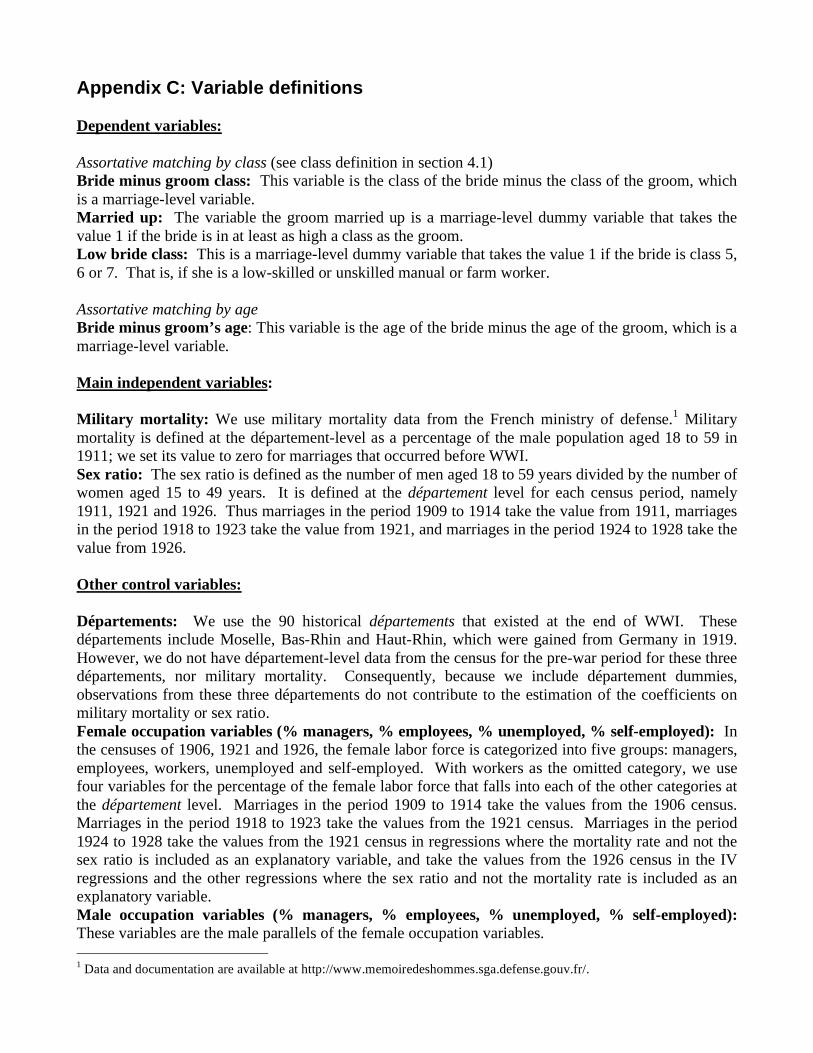
Appendix C: Variable definitions

Dependent variables: Assortative matching by class (see class definition in section 4.1)

Bride minus groom class: This variable is the class of the bride minus the class of the groom, which

is a marriage-level variable.

Married up: The variable the groom married up is a marriage-level dummy variable that takes the

value 1 if the bride is in at least as high a class as the groom.

Low bride class: This is a marriage-level dummy variable that takes the value 1 if the bride is class 5,

6 or 7. That is, if she is a low-skilled or unskilled manual or farm worker.

Assortative matching by age Bride minus groom’s age: This variable is the age of the bride minus the age of the groom, which is a

marriage-level variable.

Main independent variables:

Military mortality: We use military mortality data from the French ministry of defense.1 Military

mortality is defined at the département-level as a percentage of the male population aged 18 to 59 in

1911; we set its value to zero for marriages that occurred before WWI.

Sex ratio: The sex ratio is defined as the number of men aged 18 to 59 years divided by the number of

women aged 15 to 49 years. It is defined at the département level for each census period, namely

1911, 1921 and 1926. Thus marriages in the period 1909 to 1914 take the value from 1911, marriages

in the period 1918 to 1923 take the value from 1921, and marriages in the period 1924 to 1928 take the

value from 1926.

Other control variables:

Départements: We use the 90 historical départements that existed at the end of WWI. These

départements include Moselle, Bas-Rhin and Haut-Rhin, which were gained from Germany in 1919.

However, we do not have département-level data from the census for the pre-war period for these three

départements, nor military mortality. Consequently, because we include département dummies,

observations from these three départements do not contribute to the estimation of the coefficients on

military mortality or sex ratio.

Female occupation variables (% managers, % employees, % unemployed, % self-employed): In

the censuses of 1906, 1921 and 1926, the female labor force is categorized into five groups: managers,

employees, workers, unemployed and self-employed. With workers as the omitted category, we use

four variables for the percentage of the female labor force that falls into each of the other categories at

the département level. Marriages in the period 1909 to 1914 take the values from the 1906 census.

Marriages in the period 1918 to 1923 take the values from the 1921 census. Marriages in the period

1924 to 1928 take the values from the 1921 census in regressions where the mortality rate and not the

sex ratio is included as an explanatory variable, and take the values from the 1926 census in the IV

regressions and the other regressions where the sex ratio and not the mortality rate is included as an

explanatory variable.

Male occupation variables (% managers, % employees, % unemployed, % self-employed): These variables are the male parallels of the female occupation variables.

1 Data and documentation are available at http://www.memoiredeshommes.sga.defense.gouv.fr/.

Female population age groups (% Females 20-29, % Females 30-39, % Females 40-49): They are

calculated at the département level as percentage of the female population aged 15-49. Women aged

15 to 19 is the omitted category. Marriages in the period 1909 to 1914 take the values from the 1911

census. Marriages in the period 1918 to 1928 take the values from the 1921 census.

Excess foreign males: This variable is defined as foreign males as a percentage of total males minus

foreign females as a percentage of total females at the département level. We define as foreign all

individuals classified by the census as foreign or naturalised French, regardless of their place of birth.

Individuals classified as French by the census are considered to not be foreign, regardless of whether

they were born in France or not. Marriages in the period 1909 to 1914 take the values from the 1911

census. Marriages in the period 1918 to 1923 take the values from the 1921 census. Marriages in the

period 1924 to 1928 take the values from the 1921 census in regressions where the mortality rate and

not the sex ratio is included as an explanatory variable, and take the values from the 1926 census in the

IV regressions and the other regressions where the sex ratio and not the mortality rate is included as an

explanatory variable.

Rural: This a dummy variable defined at the marriage level. It is defined in terms of the

administrative status of the place of marriage, which may take the values chef lieu de département, chef lieu d'arrondissement, chef-lieu de canton, and rural. We consider the category rural to indicate a

rural marriage, and the other three categories to indicate urban marriages.

Groom’s age: The age of the groom is constructed from three marriage-level variables: the age of the

groom, the year of the marriage and the groom’s year of birth. If the stated age of the groom falls in

the range 10 to 89, this is the value used. If it does not, or the age of the groom is missing, we use the

difference between the year of marriage and the groom’s year of birth if this falls in the range 10 to 89.

Otherwise the groom’s age is missing.

Bride’s age: Same as groom’s age.

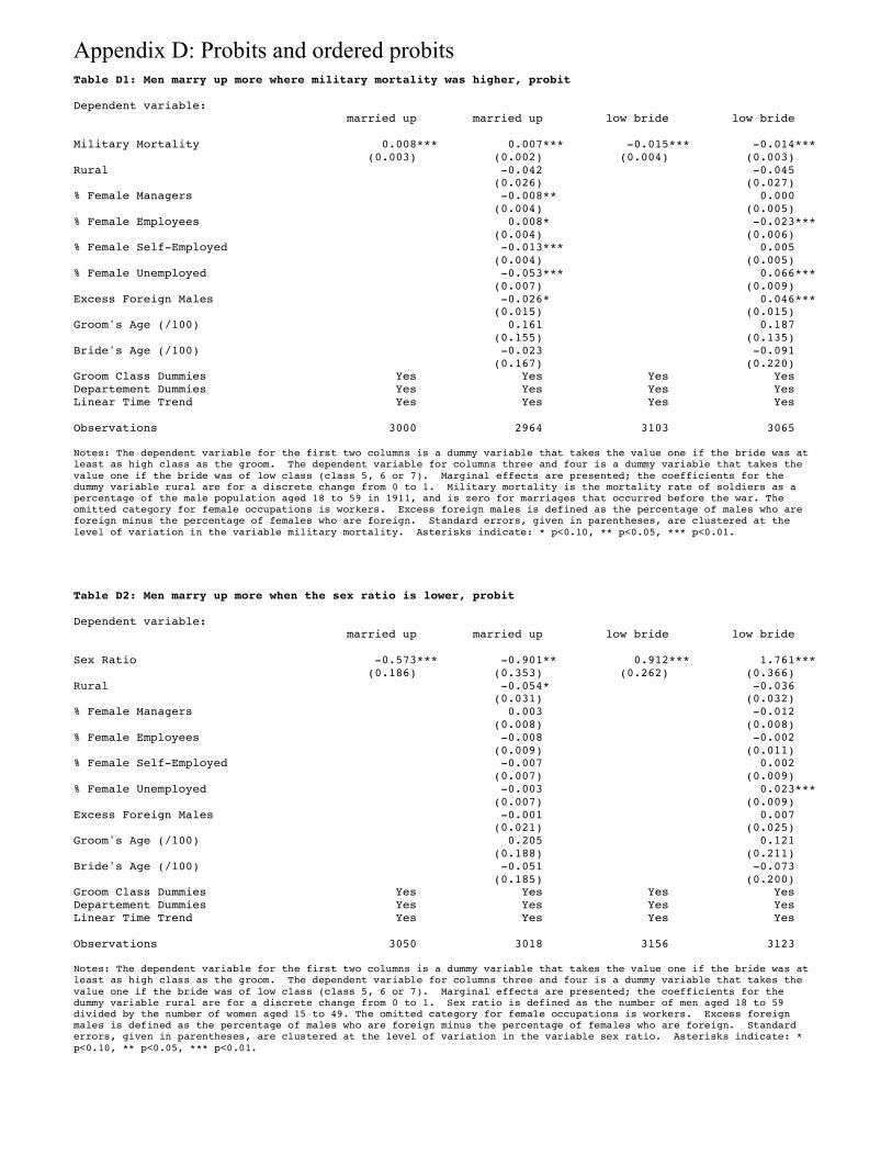
Table D1: Men marry up more where military mortality was higher, probit Dependent variable: married up married up low bride low bride Military Mortality 0.008*** 0.007*** -0.015*** -0.014*** (0.003) (0.002) (0.004) (0.003) Rural -0.042 -0.045 (0.026) (0.027) % Female Managers -0.008** 0.000 (0.004) (0.005) % Female Employees 0.008* -0.023*** (0.004) (0.006) % Female Self-Employed -0.013*** 0.005 (0.004) (0.005) % Female Unemployed -0.053*** 0.066*** (0.007) (0.009) Excess Foreign Males -0.026* 0.046*** (0.015) (0.015) Groom's Age (/100) 0.161 0.187 (0.155) (0.135) Bride's Age (/100) -0.023 -0.091 (0.167) (0.220) Groom Class Dummies Yes Yes Yes Yes Departement Dummies Yes Yes Yes Yes Linear Time Trend Yes Yes Yes Yes Observations 3000 2964 3103 3065 Notes: The dependent variable for the first two columns is a dummy variable that takes the value one if the bride was at least as high class as the groom. The dependent variable for columns three and four is a dummy variable that takes the

value one if the bride was of low class (class 5, 6 or 7). Marginal effects are presented; the coefficients for the dummy variable rural are for a discrete change from 0 to 1. Military mortality is the mortality rate of soldiers as a percentage of the male population aged 18 to 59 in 1911, and is zero for marriages that occurred before the war. The omitted category for female occupations is workers. Excess foreign males is defined as the percentage of males who are foreign minus the percentage of females who are foreign. Standard errors, given in parentheses, are clustered at the

level of variation in the variable military mortality. Asterisks indicate: * p<0.10, ** p<0.05, *** p<0.01.

Table D2: Men marry up more when the sex ratio is lower, probit Dependent variable: married up married up low bride low bride Sex Ratio -0.573*** -0.901** 0.912*** 1.761*** (0.186) (0.353) (0.262) (0.366) Rural -0.054* -0.036 (0.031) (0.032) % Female Managers 0.003 -0.012 (0.008) (0.008) % Female Employees -0.008 -0.002 (0.009) (0.011) % Female Self-Employed -0.007 0.002 (0.007) (0.009) % Female Unemployed -0.003 0.023*** (0.007) (0.009) Excess Foreign Males -0.001 0.007 (0.021) (0.025) Groom's Age (/100) 0.205 0.121 (0.188) (0.211) Bride's Age (/100) -0.051 -0.073 (0.185) (0.200) Groom Class Dummies Yes Yes Yes Yes Departement Dummies Yes Yes Yes Yes Linear Time Trend Yes Yes Yes Yes Observations 3050 3018 3156 3123 Notes: The dependent variable for the first two columns is a dummy variable that takes the value one if the bride was at least as high class as the groom. The dependent variable for columns three and four is a dummy variable that takes the

value one if the bride was of low class (class 5, 6 or 7). Marginal effects are presented; the coefficients for the dummy variable rural are for a discrete change from 0 to 1. Sex ratio is defined as the number of men aged 18 to 59 divided by the number of women aged 15 to 49. The omitted category for female occupations is workers. Excess foreign males is defined as the percentage of males who are foreign minus the percentage of females who are foreign. Standard errors, given in parentheses, are clustered at the level of variation in the variable sex ratio. Asterisks indicate: *

p<0.10, ** p<0.05, *** p<0.01.

Appendix D: Probits and ordered probits

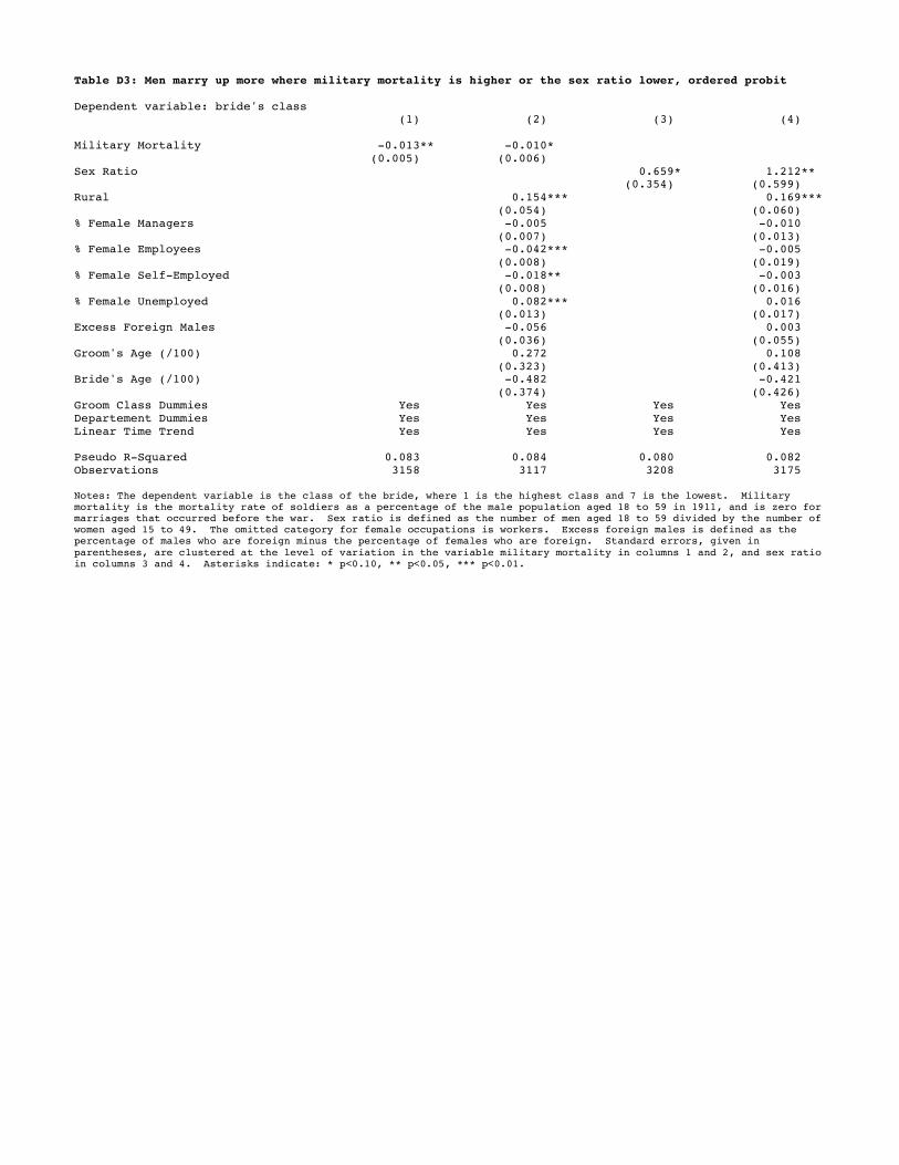
Table D3: Men marry up more where military mortality is higher or the sex ratio lower, ordered probit Dependent variable: bride's class (1) (2) (3) (4) Military Mortality -0.013** -0.010* (0.005) (0.006) Sex Ratio 0.659* 1.212** (0.354) (0.599) Rural 0.154*** 0.169*** (0.054) (0.060) % Female Managers -0.005 -0.010 (0.007) (0.013) % Female Employees -0.042*** -0.005 (0.008) (0.019) % Female Self-Employed -0.018** -0.003 (0.008) (0.016) % Female Unemployed 0.082*** 0.016 (0.013) (0.017) Excess Foreign Males -0.056 0.003 (0.036) (0.055) Groom's Age (/100) 0.272 0.108 (0.323) (0.413) Bride's Age (/100) -0.482 -0.421 (0.374) (0.426) Groom Class Dummies Yes Yes Yes Yes Departement Dummies Yes Yes Yes Yes Linear Time Trend Yes Yes Yes Yes Pseudo R-Squared 0.083 0.084 0.080 0.082 Observations 3158 3117 3208 3175 Notes: The dependent variable is the class of the bride, where 1 is the highest class and 7 is the lowest. Military mortality is the mortality rate of soldiers as a percentage of the male population aged 18 to 59 in 1911, and is zero for marriages that occurred before the war. Sex ratio is defined as the number of men aged 18 to 59 divided by the number of women aged 15 to 49. The omitted category for female occupations is workers. Excess foreign males is defined as the percentage of males who are foreign minus the percentage of females who are foreign. Standard errors, given in

parentheses, are clustered at the level of variation in the variable military mortality in columns 1 and 2, and sex ratio in columns 3 and 4. Asterisks indicate: * p<0.10, ** p<0.05, *** p<0.01.

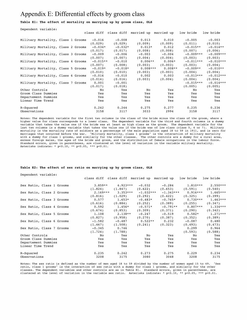
Table E1: The effect of mortality on marrying up by groom class, OLS Dependent variable: class diff class diff married up married up low bride low bride Military Mortality, Class 1 Grooms -0.016 -0.008 0.013 0.010 -0.005 -0.003 (0.029) (0.029) (0.009) (0.009) (0.011) (0.010) Military Mortality, Class 2 Grooms -0.034* -0.032* 0.013* 0.012 -0.015** -0.014** (0.017) (0.017) (0.008) (0.008) (0.007) (0.006) Military Mortality, Class 3 Grooms -0.009 -0.006 -0.003 -0.004 -0.009*** -0.009*** (0.007) (0.007) (0.004) (0.004) (0.003) (0.003) Military Mortality, Class 4 Grooms -0.015** -0.010 0.006** 0.006* -0.011*** -0.010*** (0.007) (0.008) (0.003) (0.003) (0.003) (0.004) Military Mortality, Class 5 Grooms -0.019* -0.018* 0.008*** 0.008** -0.009** -0.010** (0.010) (0.010) (0.003) (0.003) (0.004) (0.004) Military Mortality, Class 6 Grooms -0.016 -0.010 0.002 0.003 -0.013*** -0.012*** (0.014) (0.016) (0.003) (0.004) (0.004) (0.004) Military Mortality, Class 7 Grooms 0.001 -0.001 -0.015*** -0.014*** (0.017) (0.018) (0.005) (0.005) Other Controls No Yes No Yes No Yes Groom Class Dummies Yes Yes Yes Yes Yes Yes Departement Dummies Yes Yes Yes Yes Yes Yes Linear Time Trend Yes Yes Yes Yes Yes Yes R-Squared 0.242 0.244 0.275 0.277 0.235 0.236 Observations 3158 3117 3033 2994 3158 3117 Notes: The dependent variable for the first two columns is the class of the bride minus the class of the groom, where a higher value for class corresponds to a lower class. The dependent variable for the third and fourth columns is a dummy variable that takes the value one if the bride was at least as high class as the groom. The dependent variable for the last two columns is a dummy variable that takes the value one if the bride was of low class (class 5, 6 or 7). Military mortality is the mortality rate of soldiers as a percentage of the male population aged 18 to 59 in 1911, and is zero for

marriages that occurred before the war. "Military mortality, class 1 grooms" is the interaction of military mortality with a dummy for class 1 grooms, and similarly for the other classes. The other controls are a dummy for a rural area, excess foreign males, the ages of the bride and groom, and the distribution of female occupations in the labour force. Standard errors, given in parentheses, are clustered at the level of variation in the variable military mortality. Asterisks indicate: * p<0.10, ** p<0.05, *** p<0.01.

Table E2: The effect of sex ratio on marrying up by groom class, OLS Dependent variable: class diff class diff married up married up low bride low bride Sex Ratio, Class 1 Grooms 3.859** 4.923*** -0.032 -0.284 1.810*** 2.550*** (1.824) (1.847) (0.622) (0.653) (0.591) (0.540) Sex Ratio, Class 2 Grooms 2.169*** 3.353*** -1.032*** -1.343*** 0.916*** 1.665*** (0.816) (1.029) (0.292) (0.422) (0.325) (0.399) Sex Ratio, Class 3 Grooms 0.577 1.653* -0.483* -0.765* 0.730*** 1.463*** (0.616) (0.884) (0.252) (0.389) (0.255) (0.347) Sex Ratio, Class 4 Grooms 0.592 1.456* -0.571* -0.791** 0.807*** 1.334*** (0.674) (0.853) (0.309) (0.371) (0.290) (0.342) Sex Ratio, Class 5 Grooms 1.108 2.138** -0.247 -0.519 0.582* 1.271*** (0.827) (0.958) (0.270) (0.387) (0.352) (0.389) Sex Ratio, Class 6 Grooms -1.582 -0.487 0.522** 0.232 -0.087 0.480 (1.467) (1.508) (0.241) (0.323) (0.493) (0.473) Sex Ratio, Class 7 Grooms -0.345 0.746 0.299 0.964 (1.724) (1.788) (0.593) (0.588) Other Controls No Yes No Yes No Yes Groom Class Dummies Yes Yes Yes Yes Yes Yes Departement Dummies Yes Yes Yes Yes Yes Yes Linear Time Trend Yes Yes Yes Yes Yes Yes R-Squared 0.235 0.242 0.273 0.275 0.229 0.234 Observations 3208 3175 3080 3048 3208 3175 Notes: The sex ratio is defined as the number of men aged 18 to 59 divided by the number of women aged 15 to 49. "Sex ratio, class 1 grooms" is the interaction of sex ratio with a dummy for class 1 grooms, and similarly for the other

classes. The dependent variables and other controls are as in Table E1. Standard errors, given in parentheses, are clustered at the level of variation in the variable sex ratio. Asterisks indicate: * p<0.10, ** p<0.05, *** p<0.01.

Appendix E: Differential effects by groom class

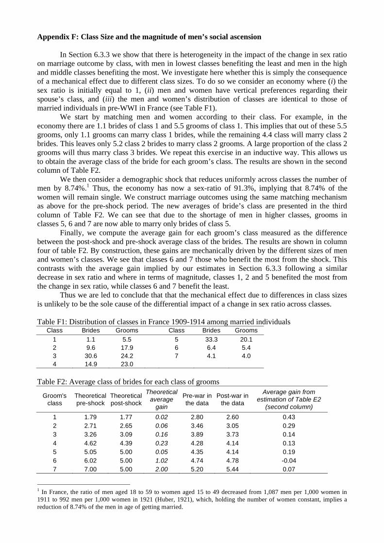
Appendix F: Class Size and the magnitude of men’s social ascension

In Section 6.3.3 we show that there is heterogeneity in the impact of the change in sex ratio

on marriage outcome by class, with men in lowest classes benefiting the least and men in the high

and middle classes benefiting the most. We investigate here whether this is simply the consequence

of a mechanical effect due to different class sizes. To do so we consider an economy where (i) the

sex ratio is initially equal to 1, (ii) men and women have vertical preferences regarding their

spouse’s class, and (iii) the men and women’s distribution of classes are identical to those of

married individuals in pre-WWI in France (see Table F1).

We start by matching men and women according to their class. For example, in the

economy there are 1.1 brides of class 1 and 5.5 grooms of class 1. This implies that out of these 5.5

grooms, only 1.1 grooms can marry class 1 brides, while the remaining 4.4 class will marry class 2

brides. This leaves only 5.2 class 2 brides to marry class 2 grooms. A large proportion of the class 2

grooms will thus marry class 3 brides. We repeat this exercise in an inductive way. This allows us

to obtain the average class of the bride for each groom’s class. The results are shown in the second

column of Table F2.

We then consider a demographic shock that reduces uniformly across classes the number of

men by 8.74%.1 Thus, the economy has now a sex-ratio of 91.3%, implying that 8.74% of the

women will remain single. We construct marriage outcomes using the same matching mechanism

as above for the pre-shock period. The new averages of bride’s class are presented in the third

column of Table F2. We can see that due to the shortage of men in higher classes, grooms in

classes 5, 6 and 7 are now able to marry only brides of class 5.

Finally, we compute the average gain for each groom’s class measured as the difference

between the post-shock and pre-shock average class of the brides. The results are shown in column

four of table F2. By construction, these gains are mechanically driven by the different sizes of men

and women’s classes. We see that classes 6 and 7 those who benefit the most from the shock. This

contrasts with the average gain implied by our estimates in Section 6.3.3 following a similar

decrease in sex ratio and where in terms of magnitude, classes 1, 2 and 5 benefited the most from

the change in sex ratio, while classes 6 and 7 benefit the least.

Thus we are led to conclude that that the mechanical effect due to differences in class sizes

is unlikely to be the sole cause of the differential impact of a change in sex ratio across classes.

Table F1: Distribution of classes in France 1909-1914 among married individuals Class Brides Grooms Class Brides Grooms

1 1.1 5.5 5 33.3 20.1 2 9.6 17.9 6 6.4 5.4 3 30.6 24.2 7 4.1 4.0 4 14.9 23.0

Table F2: Average class of brides for each class of grooms

Groom's class

Theoretical pre-shock

Theoretical post-shock

Theoretical

average

gain

Pre-war in the data

Post-war in the data

Average gain from

estimation of Table E2

(second column)

1 1.79 1.77 0.02 2.80 2.60 0.43

2 2.71 2.65 0.06 3.46 3.05 0.29

3 3.26 3.09 0.16 3.89 3.73 0.14

4 4.62 4.39 0.23 4.28 4.14 0.13

5 5.05 5.00 0.05 4.35 4.14 0.19

6 6.02 5.00 1.02 4.74 4.78 -0.04

7 7.00 5.00 2.00 5.20 5.44 0.07

1 In France, the ratio of men aged 18 to 59 to women aged 15 to 49 decreased from 1,087 men per 1,000 women in

1911 to 992 men per 1,000 women in 1921 (Huber, 1921), which, holding the number of women constant, implies a

reduction of 8.74% of the men in age of getting married.

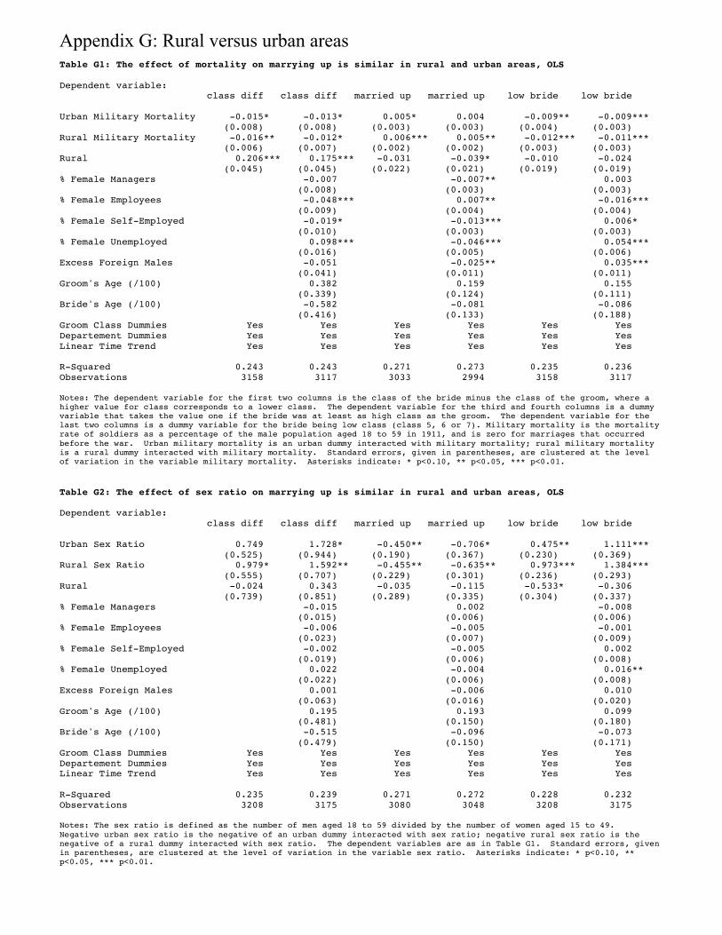
Table G1: The effect of mortality on marrying up is similar in rural and urban areas, OLS Dependent variable: class diff class diff married up married up low bride low bride Urban Military Mortality -0.015* -0.013* 0.005* 0.004 -0.009** -0.009*** (0.008) (0.008) (0.003) (0.003) (0.004) (0.003) Rural Military Mortality -0.016** -0.012* 0.006*** 0.005** -0.012*** -0.011*** (0.006) (0.007) (0.002) (0.002) (0.003) (0.003) Rural 0.206*** 0.175*** -0.031 -0.039* -0.010 -0.024 (0.045) (0.045) (0.022) (0.021) (0.019) (0.019) % Female Managers -0.007 -0.007** 0.003 (0.008) (0.003) (0.003) % Female Employees -0.048*** 0.007** -0.016*** (0.009) (0.004) (0.004) % Female Self-Employed -0.019* -0.013*** 0.006* (0.010) (0.003) (0.003) % Female Unemployed 0.098*** -0.046*** 0.054*** (0.016) (0.005) (0.006) Excess Foreign Males -0.051 -0.025** 0.035*** (0.041) (0.011) (0.011) Groom's Age (/100) 0.382 0.159 0.155 (0.339) (0.124) (0.111) Bride's Age (/100) -0.582 -0.081 -0.086 (0.416) (0.133) (0.188) Groom Class Dummies Yes Yes Yes Yes Yes Yes Departement Dummies Yes Yes Yes Yes Yes Yes Linear Time Trend Yes Yes Yes Yes Yes Yes R-Squared 0.243 0.243 0.271 0.273 0.235 0.236 Observations 3158 3117 3033 2994 3158 3117 Notes: The dependent variable for the first two columns is the class of the bride minus the class of the groom, where a higher value for class corresponds to a lower class. The dependent variable for the third and fourth columns is a dummy variable that takes the value one if the bride was at least as high class as the groom. The dependent variable for the last two columns is a dummy variable for the bride being low class (class 5, 6 or 7). Military mortality is the mortality rate of soldiers as a percentage of the male population aged 18 to 59 in 1911, and is zero for marriages that occurred

before the war. Urban military mortality is an urban dummy interacted with military mortality; rural military mortality is a rural dummy interacted with military mortality. Standard errors, given in parentheses, are clustered at the level of variation in the variable military mortality. Asterisks indicate: * p<0.10, ** p<0.05, *** p<0.01.

Table G2: The effect of sex ratio on marrying up is similar in rural and urban areas, OLS Dependent variable: class diff class diff married up married up low bride low bride Urban Sex Ratio 0.749 1.728* -0.450** -0.706* 0.475** 1.111*** (0.525) (0.944) (0.190) (0.367) (0.230) (0.369) Rural Sex Ratio 0.979* 1.592** -0.455** -0.635** 0.973*** 1.384*** (0.555) (0.707) (0.229) (0.301) (0.236) (0.293) Rural -0.024 0.343 -0.035 -0.115 -0.533* -0.306 (0.739) (0.851) (0.289) (0.335) (0.304) (0.337) % Female Managers -0.015 0.002 -0.008 (0.015) (0.006) (0.006) % Female Employees -0.006 -0.005 -0.001 (0.023) (0.007) (0.009) % Female Self-Employed -0.002 -0.005 0.002 (0.019) (0.006) (0.008) % Female Unemployed 0.022 -0.004 0.016** (0.022) (0.006) (0.008) Excess Foreign Males 0.001 -0.006 0.010 (0.063) (0.016) (0.020) Groom's Age (/100) 0.195 0.193 0.099 (0.481) (0.150) (0.180) Bride's Age (/100) -0.515 -0.096 -0.073 (0.479) (0.150) (0.171) Groom Class Dummies Yes Yes Yes Yes Yes Yes Departement Dummies Yes Yes Yes Yes Yes Yes Linear Time Trend Yes Yes Yes Yes Yes Yes R-Squared 0.235 0.239 0.271 0.272 0.228 0.232 Observations 3208 3175 3080 3048 3208 3175 Notes: The sex ratio is defined as the number of men aged 18 to 59 divided by the number of women aged 15 to 49.

Negative urban sex ratio is the negative of an urban dummy interacted with sex ratio; negative rural sex ratio is the negative of a rural dummy interacted with sex ratio. The dependent variables are as in Table G1. Standard errors, given in parentheses, are clustered at the level of variation in the variable sex ratio. Asterisks indicate: * p<0.10, ** p<0.05, *** p<0.01.

Appendix G: Rural versus urban areas

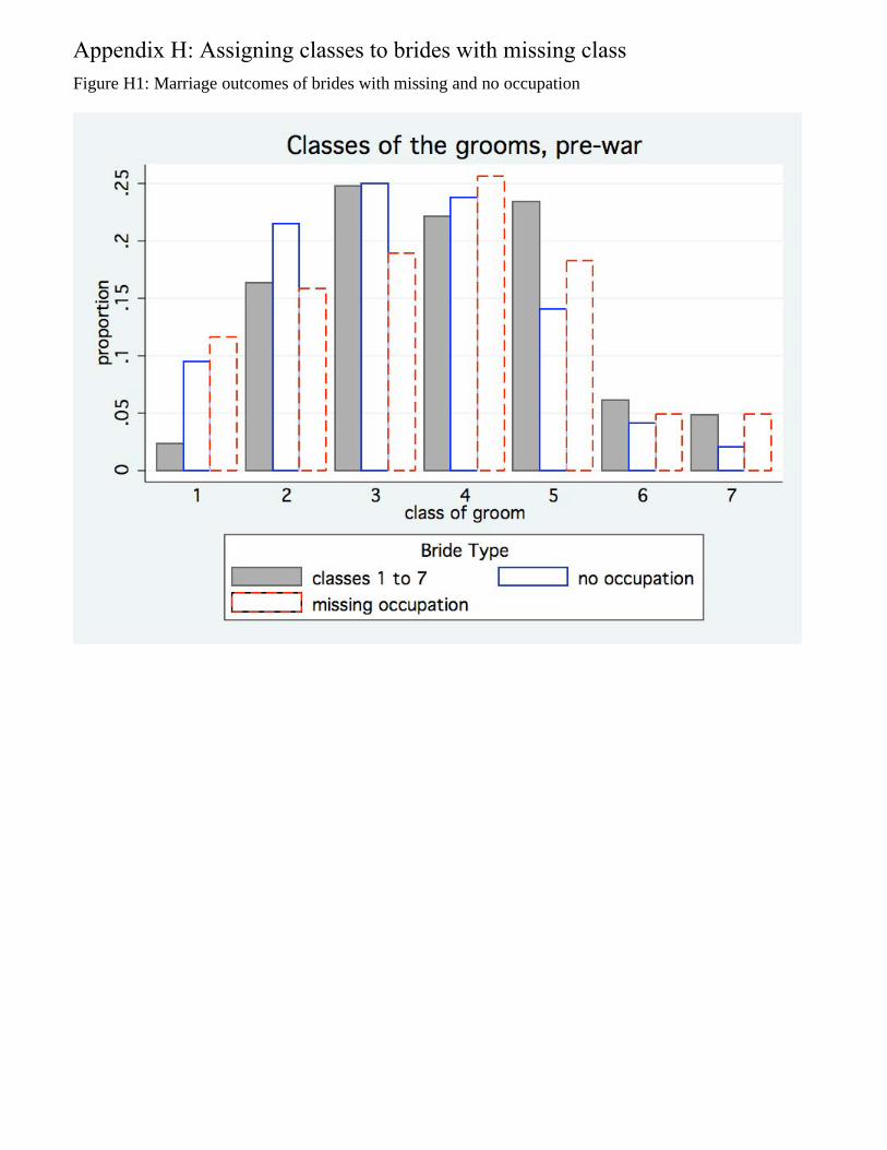
Figure H1: Marriage outcomes of brides with missing and no occupation

Appendix H: Assigning classes to brides with missing class

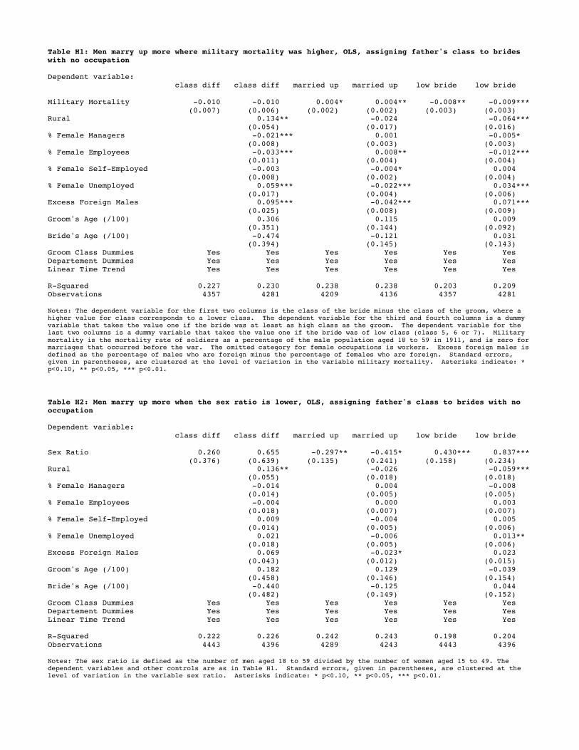
Table H1: Men marry up more where military mortality was higher, OLS, assigning father's class to brides with no occupation Dependent variable: class diff class diff married up married up low bride low bride Military Mortality -0.010 -0.010 0.004* 0.004** -0.008** -0.009*** (0.007) (0.006) (0.002) (0.002) (0.003) (0.003) Rural 0.134** -0.024 -0.064*** (0.054) (0.017) (0.016) % Female Managers -0.021*** 0.001 -0.005* (0.008) (0.003) (0.003) % Female Employees -0.033*** 0.008** -0.012*** (0.011) (0.004) (0.004) % Female Self-Employed -0.003 -0.004* 0.004 (0.008) (0.002) (0.004) % Female Unemployed 0.059*** -0.022*** 0.034*** (0.017) (0.004) (0.006) Excess Foreign Males 0.095*** -0.042*** 0.071*** (0.025) (0.008) (0.009) Groom's Age (/100) 0.306 0.115 0.009 (0.351) (0.144) (0.092) Bride's Age (/100) -0.474 -0.121 0.031 (0.394) (0.145) (0.143) Groom Class Dummies Yes Yes Yes Yes Yes Yes Departement Dummies Yes Yes Yes Yes Yes Yes Linear Time Trend Yes Yes Yes Yes Yes Yes R-Squared 0.227 0.230 0.238 0.238 0.203 0.209 Observations 4357 4281 4209 4136 4357 4281 Notes: The dependent variable for the first two columns is the class of the bride minus the class of the groom, where a higher value for class corresponds to a lower class. The dependent variable for the third and fourth columns is a dummy variable that takes the value one if the bride was at least as high class as the groom. The dependent variable for the last two columns is a dummy variable that takes the value one if the bride was of low class (class 5, 6 or 7). Military

mortality is the mortality rate of soldiers as a percentage of the male population aged 18 to 59 in 1911, and is zero for marriages that occurred before the war. The omitted category for female occupations is workers. Excess foreign males is defined as the percentage of males who are foreign minus the percentage of females who are foreign. Standard errors, given in parentheses, are clustered at the level of variation in the variable military mortality. Asterisks indicate: * p<0.10, ** p<0.05, *** p<0.01.

Table H2: Men marry up more when the sex ratio is lower, OLS, assigning father's class to brides with no occupation Dependent variable: class diff class diff married up married up low bride low bride Sex Ratio 0.260 0.655 -0.297** -0.415* 0.430*** 0.837*** (0.376) (0.639) (0.135) (0.241) (0.158) (0.234) Rural 0.136** -0.026 -0.059*** (0.055) (0.018) (0.018) % Female Managers -0.014 0.004 -0.008 (0.014) (0.005) (0.005) % Female Employees -0.004 0.000 0.003 (0.018) (0.007) (0.007) % Female Self-Employed 0.009 -0.004 0.005 (0.014) (0.005) (0.006) % Female Unemployed 0.021 -0.006 0.013** (0.018) (0.005) (0.006) Excess Foreign Males 0.069 -0.023* 0.023 (0.043) (0.012) (0.015) Groom's Age (/100) 0.182 0.129 -0.039 (0.458) (0.146) (0.154) Bride's Age (/100) -0.440 -0.125 0.044 (0.482) (0.149) (0.152) Groom Class Dummies Yes Yes Yes Yes Yes Yes Departement Dummies Yes Yes Yes Yes Yes Yes Linear Time Trend Yes Yes Yes Yes Yes Yes R-Squared 0.222 0.226 0.242 0.243 0.198 0.204 Observations 4443 4396 4289 4243 4443 4396 Notes: The sex ratio is defined as the number of men aged 18 to 59 divided by the number of women aged 15 to 49. The dependent variables and other controls are as in Table H1. Standard errors, given in parentheses, are clustered at the level of variation in the variable sex ratio. Asterisks indicate: * p<0.10, ** p<0.05, *** p<0.01.

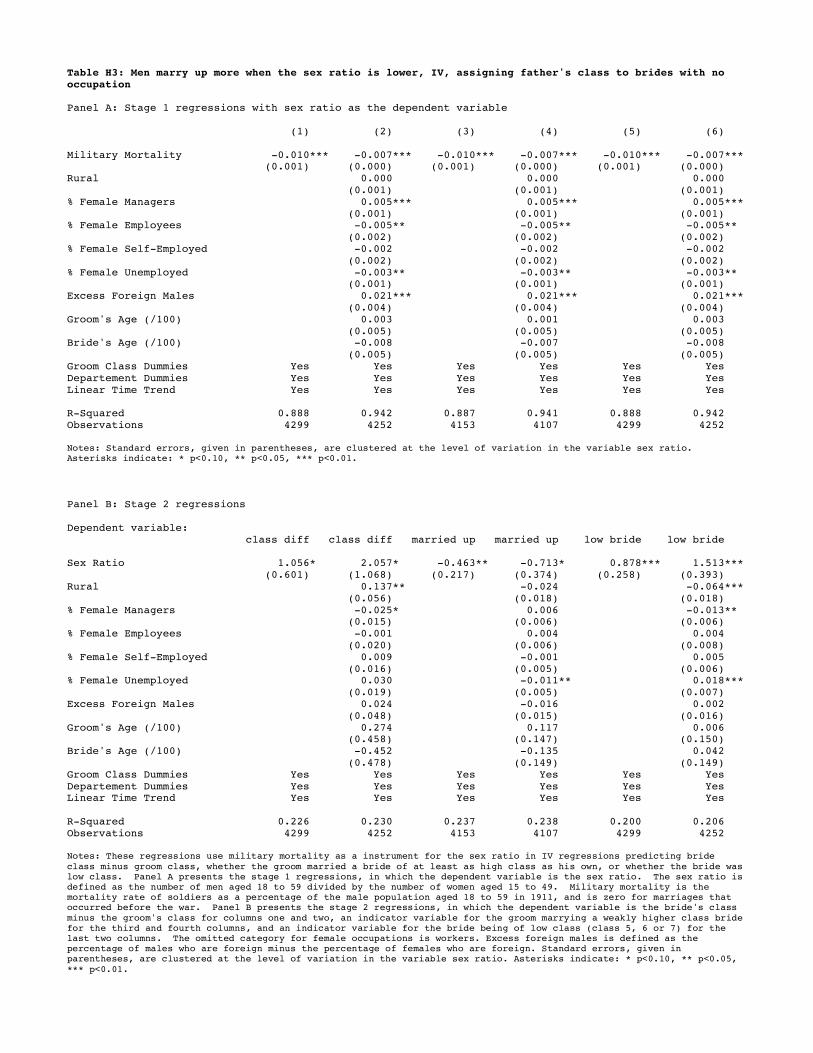
Table H3: Men marry up more when the sex ratio is lower, IV, assigning father's class to brides with no occupation Panel A: Stage 1 regressions with sex ratio as the dependent variable (1) (2) (3) (4) (5) (6) Military Mortality -0.010*** -0.007*** -0.010*** -0.007*** -0.010*** -0.007*** (0.001) (0.000) (0.001) (0.000) (0.001) (0.000) Rural 0.000 0.000 0.000 (0.001) (0.001) (0.001) % Female Managers 0.005*** 0.005*** 0.005*** (0.001) (0.001) (0.001) % Female Employees -0.005** -0.005** -0.005** (0.002) (0.002) (0.002) % Female Self-Employed -0.002 -0.002 -0.002 (0.002) (0.002) (0.002) % Female Unemployed -0.003** -0.003** -0.003** (0.001) (0.001) (0.001) Excess Foreign Males 0.021*** 0.021*** 0.021*** (0.004) (0.004) (0.004) Groom's Age (/100) 0.003 0.001 0.003 (0.005) (0.005) (0.005) Bride's Age (/100) -0.008 -0.007 -0.008 (0.005) (0.005) (0.005) Groom Class Dummies Yes Yes Yes Yes Yes Yes Departement Dummies Yes Yes Yes Yes Yes Yes Linear Time Trend Yes Yes Yes Yes Yes Yes R-Squared 0.888 0.942 0.887 0.941 0.888 0.942 Observations 4299 4252 4153 4107 4299 4252 Notes: Standard errors, given in parentheses, are clustered at the level of variation in the variable sex ratio. Asterisks indicate: * p<0.10, ** p<0.05, *** p<0.01.

Panel B: Stage 2 regressions Dependent variable: class diff class diff married up married up low bride low bride Sex Ratio 1.056* 2.057* -0.463** -0.713* 0.878*** 1.513*** (0.601) (1.068) (0.217) (0.374) (0.258) (0.393) Rural 0.137** -0.024 -0.064*** (0.056) (0.018) (0.018) % Female Managers -0.025* 0.006 -0.013** (0.015) (0.006) (0.006) % Female Employees -0.001 0.004 0.004 (0.020) (0.006) (0.008) % Female Self-Employed 0.009 -0.001 0.005 (0.016) (0.005) (0.006) % Female Unemployed 0.030 -0.011** 0.018*** (0.019) (0.005) (0.007) Excess Foreign Males 0.024 -0.016 0.002 (0.048) (0.015) (0.016) Groom's Age (/100) 0.274 0.117 0.006 (0.458) (0.147) (0.150) Bride's Age (/100) -0.452 -0.135 0.042 (0.478) (0.149) (0.149) Groom Class Dummies Yes Yes Yes Yes Yes Yes Departement Dummies Yes Yes Yes Yes Yes Yes Linear Time Trend Yes Yes Yes Yes Yes Yes R-Squared 0.226 0.230 0.237 0.238 0.200 0.206 Observations 4299 4252 4153 4107 4299 4252 Notes: These regressions use military mortality as a instrument for the sex ratio in IV regressions predicting bride

class minus groom class, whether the groom married a bride of at least as high class as his own, or whether the bride was low class. Panel A presents the stage 1 regressions, in which the dependent variable is the sex ratio. The sex ratio is defined as the number of men aged 18 to 59 divided by the number of women aged 15 to 49. Military mortality is the mortality rate of soldiers as a percentage of the male population aged 18 to 59 in 1911, and is zero for marriages that occurred before the war. Panel B presents the stage 2 regressions, in which the dependent variable is the bride's class

minus the groom's class for columns one and two, an indicator variable for the groom marrying a weakly higher class bride for the third and fourth columns, and an indicator variable for the bride being of low class (class 5, 6 or 7) for the last two columns. The omitted category for female occupations is workers. Excess foreign males is defined as the percentage of males who are foreign minus the percentage of females who are foreign. Standard errors, given in parentheses, are clustered at the level of variation in the variable sex ratio. Asterisks indicate: * p<0.10, ** p<0.05,

*** p<0.01.

Table H4: The imputation of bride class, OLS

Dependent variable: Bride's class

Coefficient Std. Error

Class 1 Father -0.815*** 0.230

Class 2 Father -0.560*** 0.131

Class 3 Father -0.109 0.119

Class 4 Father 0.192 0.139

Class 5 Father 0.303** 0.125

Class 6 Father 0.488*** 0.130

Class 7 Father 0.456 0.318

Class 1 Mother -0.502 0.347

Class 2 Mother -0.726*** 0.177

Class 3 Mother -0.646*** 0.149

Class 4 Mother 0.034 0.153

Class 5 Mother 0.238** 0.100

Class 6 Mother 0.551*** 0.151

Class 7 Mother -0.921 1.301

Father has missing occupation because he's dead 0.052 0.098

Mother has missing occupation because she's dead 0.032 0.090

Father has no Occupation -0.117 0.245

Mother has no Occupation -0.292*** 0.093

Rural 0.517*** 0.148

Rural Interacted With:

Class 1 Father 0.202 0.384

Class 2 Father -0.289 0.295

Class 3 Father -0.576** 0.227

Class 4 Father -0.287 0.192

Class 5 Father -0.234 0.216

Class 6 Father 0.103 0.334

Class 7 Father -0.241 0.364

Class 1 Mother 0.234 0.562

Class 2 Mother 0.202 0.398

Class 3 Mother 0.665** 0.329

Class 4 Mother -0.165 0.195

Class 5 Mother 0.141 0.159

Class 6 Mother 0.284 0.366

Class 7 Mother 1.538 1.317

Father has missing occupation because he's dead -0.174 0.164

Mother has missing occupation because she's dead 0.177 0.151

Father has no Occupation 1.153* 0.691

Mother has no Occupation -0.150 0.182

Paris -0.382*** 0.075

Big City -0.154 0.106

Medium Sized City 0.045 0.079

Bride's Age -0.068*** 0.016

Bride's Age Squared 0.098*** 0.024

Linear Time Trend -0.009** 0.004

Observations 3312

R-squared 0.1707

Notes: The omitted category for parent's class is missing class for unknown reason. The omitted category for city size is small city or other area. Asterisks indicate: * 10%, ** 5%, ***1%.

Table H5: Men marry up more where military mortality was higher, OLS, imputing class for brides with missing class Dependent variable: class diff class diff married up married up low bride low bride Military Mortality -0.009** -0.009** 0.004*** 0.005*** -0.008*** -0.008*** (0.004) (0.004) (0.002) (0.002) (0.002) (0.001) Rural 0.302*** -0.069*** 0.061*** (0.034) (0.011) (0.017) % Female Managers -0.016*** 0.001 -0.012*** (0.004) (0.002) (0.002) % Female Employees -0.035*** 0.011*** -0.015*** (0.005) (0.002) (0.003) % Female Self-Employed -0.016*** 0.002 -0.005** (0.004) (0.002) (0.002) % Female Unemployed 0.039*** -0.015*** 0.022*** (0.008) (0.003) (0.004) Excess Foreign Males 0.029** -0.040*** 0.030*** (0.014) (0.004) (0.007) Groom's Age (/100) 0.340 0.163 -0.027 (0.212) (0.115) (0.082) Bride's Age (/100) -0.262 -0.159 0.063 (0.269) (0.116) (0.112) Groom Class Dummies Yes Yes Yes Yes Yes Yes Departement Dummies Yes Yes Yes Yes Yes Yes Linear Time Trend Yes Yes Yes Yes Yes Yes R-Squared 0.212 0.222 0.418 0.419 0.164 0.168 Observations 5593 5498 5408 5318 5593 5498 Notes: The dependent variable for the first two columns is the class of the bride minus the class of the groom, where a higher value for class corresponds to a lower class. The dependent variable for the third and fourth columns is a dummy variable that takes the value one if the bride was at least as high class as the groom. The dependent variable for the last two columns is a dummy variable that takes the value one if the bride was of low class (class 5, 6 or 7). Military

mortality is the mortality rate of soldiers as a percentage of the male population aged 18 to 59 in 1911, and is zero for marriages that occurred before the war. The omitted category for female occupations is workers. Excess foreign males is defined as the percentage of males who are foreign minus the percentage of females who are foreign. Standard errors, given in parentheses, are clustered at the level of variation in the variable military mortality. Asterisks indicate: * p<0.10, ** p<0.05, *** p<0.01.

Table H6: Men marry up more when the sex ratio is lower, OLS, imputing class for brides with missing class Dependent variable: class diff class diff married up married up low bride low bride Sex Ratio 0.513** 0.772** -0.305*** -0.290 0.430*** 0.650*** (0.248) (0.380) (0.111) (0.179) (0.123) (0.191) Rural 0.305*** -0.069*** 0.060*** (0.038) (0.014) (0.017) % Female Managers -0.014* 0.002 -0.009** (0.008) (0.004) (0.004) % Female Employees -0.013 -0.001 -0.001 (0.011) (0.005) (0.006) % Female Self-Employed -0.003 -0.003 0.000 (0.008) (0.004) (0.005) % Female Unemployed 0.014 -0.000 0.006 (0.010) (0.004) (0.005) Excess Foreign Males 0.029 -0.013 0.012 (0.027) (0.010) (0.011) Groom's Age (/100) 0.227 0.178* -0.056 (0.268) (0.105) (0.121) Bride's Age (/100) -0.232 -0.161 0.031 (0.306) (0.114) (0.134) Groom Class Dummies Yes Yes Yes Yes Yes Yes Departement Dummies Yes Yes Yes Yes Yes Yes Linear Time Trend Yes Yes Yes Yes Yes Yes R-Squared 0.205 0.218 0.419 0.423 0.159 0.164 Observations 5729 5682 5532 5486 5729 5682 Notes: The dependent variable for the first two columns is the class of the bride minus the class of the groom, where a higher value for class corresponds to a lower class. The dependent variable for the third and fourth columns is a dummy

variable that takes the value one if the bride was at least as high class as the groom. The dependent variable for the last two columns is a dummy variable that takes the value one if the bride was of low class (class 5, 6 or 7). The sex ratio is defined as the number of men aged 18 to 59 divided by the number of women aged 15 to 49. The omitted category for female occupations is workers. Excess foreign males is defined as the percentage of males who are foreign minus the percentage of females who are foreign. Standard errors, given in parentheses, are clustered at the level of variation in

the variable sex ratio. Asterisks indicate: * p<0.10, ** p<0.05, *** p<0.01.

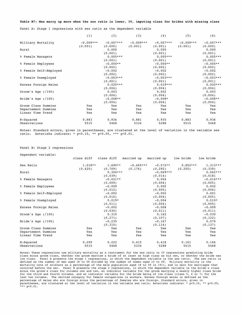
Table H7: Men marry up more when the sex ratio is lower, IV, imputing class for brides with missing class Panel A: Stage 1 regressions with sex ratio as the dependent variable (1) (2) (3) (4) (5) (6) Military Mortality -0.009*** -0.007*** -0.009*** -0.007*** -0.009*** -0.007*** (0.001) (0.000) (0.001) (0.001) (0.001) (0.000) Rural 0.000 0.000 0.000 (0.001) (0.001) (0.001) % Female Managers 0.005*** 0.005*** 0.005*** (0.001) (0.001) (0.001) % Female Employees -0.004** -0.004** -0.004** (0.002) (0.002) (0.002) % Female Self-Employed -0.002 -0.002 -0.002 (0.002) (0.002) (0.002) % Female Unemployed -0.003*** -0.003*** -0.003*** (0.001) (0.001) (0.001) Excess Foreign Males 0.020*** 0.019*** 0.020*** (0.004) (0.004) (0.004) Groom's Age (/100) 0.003 0.002 0.003 (0.004) (0.004) (0.004) Bride's Age (/100) -0.008** -0.008* -0.008** (0.004) (0.004) (0.004) Groom Class Dummies Yes Yes Yes Yes Yes Yes Departement Dummies Yes Yes Yes Yes Yes Yes Linear Time Trend Yes Yes Yes Yes Yes Yes R-Squared 0.883 0.936 0.881 0.935 0.883 0.936 Observations 5515 5468 5334 5288 5515 5468 Notes: Standard errors, given in parentheses, are clustered at the level of variation in the variable sex ratio. Asterisks indicate: * p<0.10, ** p<0.05, *** p<0.01. Panel B: Stage 2 regressions Dependent variable: class diff class diff married up married up low bride low bride Sex Ratio 1.018** 1.690** -0.465*** -0.572** 0.852*** 1.313*** (0.420) (0.709) (0.176) (0.292) (0.205) (0.339) Rural 0.304*** -0.069*** 0.062*** (0.039) (0.014) (0.018) % Female Managers -0.021** 0.004 -0.014*** (0.009) (0.004) (0.005) % Female Employees -0.009 0.000 0.002 (0.012) (0.005) (0.006) % Female Self-Employed -0.002 -0.002 0.001 (0.010) (0.004) (0.005) % Female Unemployed 0.019* -0.004 0.010* (0.011) (0.004) (0.005) Excess Foreign Males -0.002 -0.008 -0.009 (0.030) (0.011) (0.011) Groom's Age (/100) 0.310 0.162 -0.030 (0.271) (0.107) (0.122) Bride's Age (/100) -0.235 -0.167 0.070 (0.310) (0.114) (0.137) Groom Class Dummies Yes Yes Yes Yes Yes Yes Departement Dummies Yes Yes Yes Yes Yes Yes Linear Time Trend Yes Yes Yes Yes Yes Yes R-Squared 0.209 0.222 0.415 0.418 0.161 0.166 Observations 5515 5468 5334 5288 5515 5468 Notes: These regressions use military mortality as a instrument for the sex ratio in IV regressions predicting bride class minus groom class, whether the groom married a bride of at least as high class as his own, or whether the bride was low class. Panel A presents the stage 1 regressions, in which the dependent variable is the sex ratio. The sex ratio is defined as the number of men aged 18 to 59 divided by the number of women aged 15 to 49. Military mortality is the

mortality rate of soldiers as a percentage of the male population aged 18 to 59 in 1911, and is zero for marriages that occurred before the war. Panel B presents the stage 2 regressions, in which the dependent variable is the bride's class minus the groom's class for columns one and two, an indicator variable for the groom marrying a weakly higher class bride for the third and fourth columns, and an indicator variable for the bride being of low class (class 5, 6 or 7) for the last two columns. The omitted category for female occupations is workers. Excess foreign males is defined as the

percentage of males who are foreign minus the percentage of females who are foreign. Standard errors, given in parentheses, are clustered at the level of variation in the variable sex ratio. Asterisks indicate: * p<0.10, ** p<0.05, *** p<0.01.