Mass Estimators in Astrophysics

One of the most fundamental physical parameters of astrophysical systems is their mass. There are several techniques used to estimate masses (absolute measures are only possible in a few very well defined cases) that rely on the general balance between gravity and motion in systems that are in equilibrium.

Mass Estimators:The simplest case = Bound Circular Orbit Consider a test particle in orbit, mass m,

velocity v, radius R, around a body of mass M

½ mv2 = GmM/R M = ½ v2 R /GThis formula gets modified for elliptical orbits.

What about complex systems of particles?

For Multi-Object Systems

There are several estimators we use, the two most popular (and simplest) are the Virial Estimator, which is based on the Virial Theorem, and the Projected Mass Estimator.

For these estimators, all you need are the positions and velocities of the test particles (e.g. the galaxies in the system). The velocities we measure are usually only the

Line-of-sight (l.o.s.) Velocities, so some

correction must be made to account for velocities (and thus energy) perpendicular to the l.o.s. Ditto, the positions of objects we usually measure are just the positions on the plane of the sky, so some correction needs to be made for physical separations along the l.o.s.

We usually simplify by assuming that our systems are spherical.

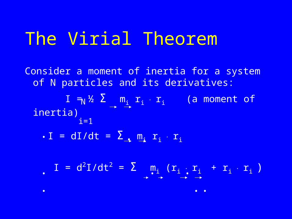
The Virial Theorem

Consider a moment of inertia for a system of N particles and its derivatives:

I = ½ Σ mi ri . ri (a moment of inertia)

I = dI/dt = Σ mi ri . ri

I = d2I/dt2 = Σ mi (ri . ri + ri

. ri )

i=1

N

..

.. . . ..

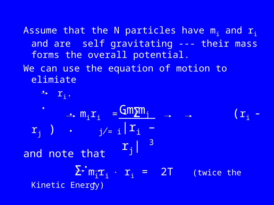
Assume that the N particles have mi and ri and

are self gravitating --- their mass forms the overall potential.

We can use the equation of motion to elimiate

ri.

miri = Σ (ri - rj )

and note that

Σ miri . ri = 2T (twice the Kinetic Energy)

..

|ri –rj| 3

j = i

Gmimj..

. .

Then we can write (after substitution)

I – 2T = Σ Σ ri . (ri – rj)

= Σ Σ rj . (rj – ri)

= ½ Σ Σ (ri - rj).(ri – rj)

= ½ Σ Σ = U the potential energy

.. i j=i

Gmi mj

|ri - rj|3

Gmi mjj i=j|rj - ri|

3

reversing labels

Gmi mj|ri - rj|

3i j=iadding

Gmi mj

|ri - rj|

∴ I = 2T + U

If we have a relaxed (or statistically steady) system which is not changing shape or size, d2I/dt2 = I = 0

2T + U = 0; U = -2T; E = T+U = ½ U

conversely, for a slowly changing or periodic system 2 <T> + <U> = 0

..

..

Virial Equilibrium

Virial Mass Estimator

We use the Virial Theorem to estimate masses of astrophysical systems (e.g. Zwicky and Smith and the discovery of Dark Matter)

Go back to:

Σ mi<vi2> = ΣΣ Gmimj < >

where < > denotes the time average, and we have N point masses of mass mi, position ri

and velocity vi

N

i=1

N

i=1 j<i

1

|ri – rj|

The observables are (1) the l.o.s. time average

velocity:

< v2R,i> Ω = 1/3 vi

2

projected radial averaged over solid angle Ω

i.e. we only see the radial component of motion &

vi ~ √3 vr

Ditto for position, we see projected radii,

R = θ d , d = distance, θ = angular separation

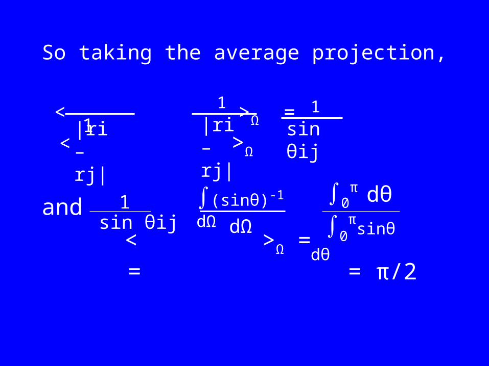
So taking the average projection,

< >Ω = < >Ω

and

< >Ω = = = π/2

1|ri – rj| |ri – rj|

1 1

sin θij

1sin θij

∫(sinθ)-1 dΩ

dΩ

∫0π dθ

∫0πsinθ dθ

Thus after taking into account all the projection effects, and if we assume masses are the same so that Msys = Σ mi = N mi we have

MVT = N

this is the Virial Theorem Mass Estimator

Σ vi2 = Velocity dispersion

[ Σ (1/Rij)]-1 = Harmonic Radius

3π2 G Σ (1/Rij)i<j

i<j

Σ vi2

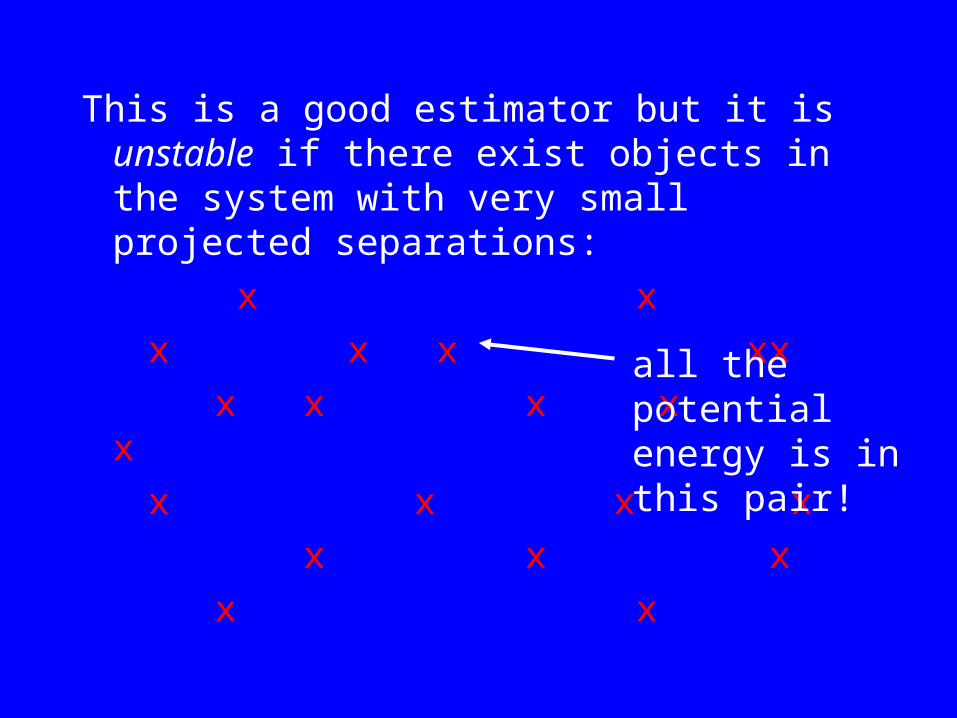
This is a good estimator but it is unstable if there exist objects in the system with very small projected separations:

x x

x x x xx

x x x x x

x x x x

x x x

x x

all the potential energy is in this pair!

Projected Mass Estimator

In the 1980’s, the search for a stable mass estimator led Bahcall & Tremaine and eventually Heisler, Bahcall & tremaine to posit a new estimator with the form

~ [dispersion x size ]

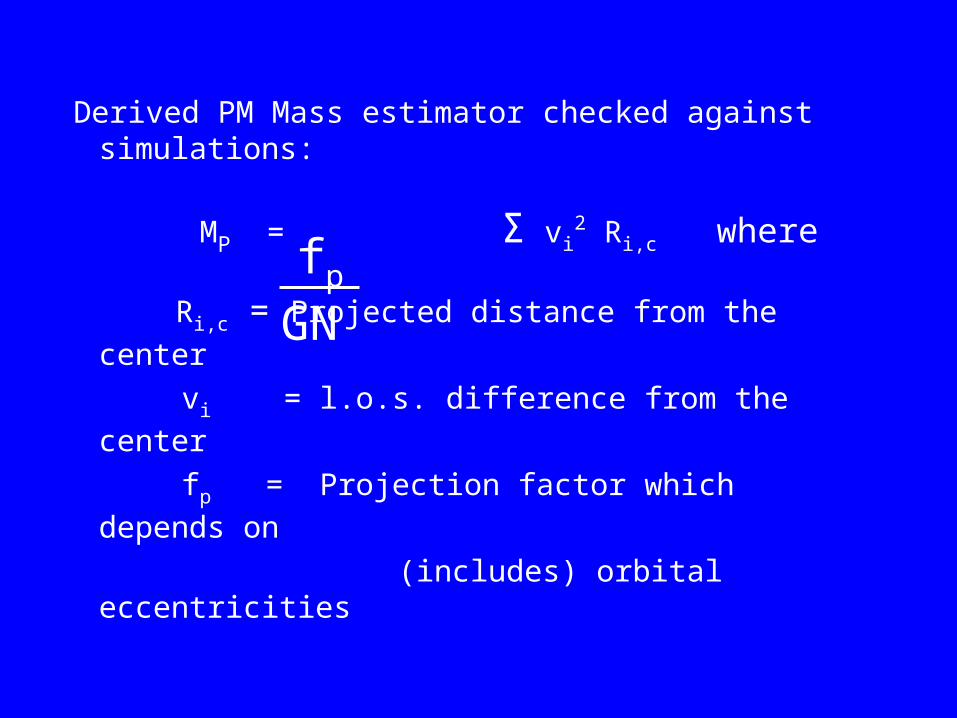
Derived PM Mass estimator checked against simulations:

MP = Σ vi2 Ri,c where

Ri,c = Projected distance from the center

vi = l.o.s. difference from the center

fp = Projection factor which depends on

(includes) orbital eccentricities

fp

GN

The projection factor depends fairly strongly on the average eccentricities of the orbits of the objects (galaxies, stars, clusters) in the system:

fp = 32/π for primarily Radial Orbits

= 16/π for primarily Isotropic Orbits = 8/π for primarily Circular OrbitsRichstone and Tremaine plotted the effect ofeccentricity vs radius on the velocity

dispersion profile:

Richstone & Tremaine

Expected projected l.o.s. sigmas

Applications:

Coma Cluster

σ ~ 1000 km/s MVT = 1.69 x 1015 MSun

MPM = 1.75 x 1015 MSun

M31 Globular Cluster System

σ ~ 155 km/s MPM = 3.10.5 x 1011 MSun

The Coma Cluster

Andromeda Galaxy = M31

M31 Globular Clusters

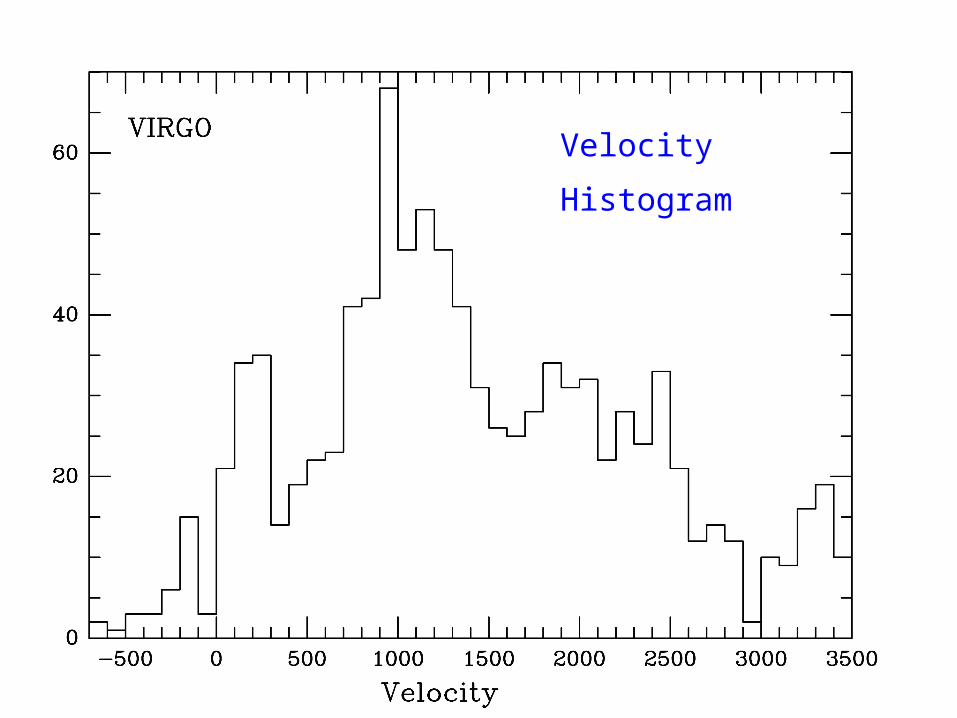
Velocity Histogram