Massive MIMO

Fundamentals, Trends and Recent Developments

Luca Sanguinetti, Emil Bjornson

University of Pisa, Italy; luca.sanguinetti@unipi.it

Linkoping University, Sweden; emil.bjornson@liu.se

ISWCS 2018, Lisbon, Aug. 28, 2018

1

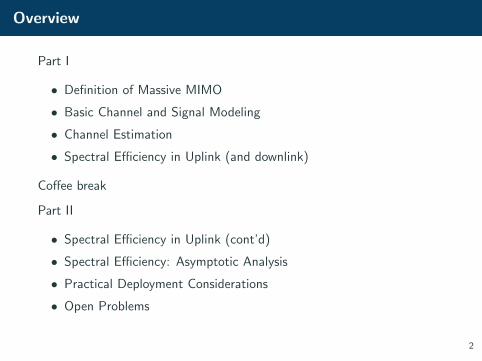
Overview

Part I

• Definition of Massive MIMO

• Basic Channel and Signal Modeling

• Channel Estimation

• Spectral Efficiency in Uplink (and downlink)

Coffee break

Part II

• Spectral Efficiency in Uplink (cont’d)

• Spectral Efficiency: Asymptotic Analysis

• Practical Deployment Considerations

• Open Problems

2

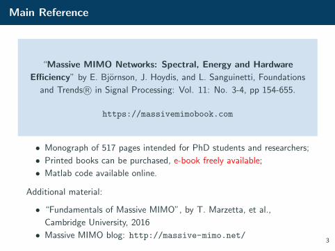
Main Reference

“Massive MIMO Networks: Spectral, Energy and Hardware

Efficiency” by E. Bjornson, J. Hoydis, and L. Sanguinetti, Foundations

and Trends R© in Signal Processing: Vol. 11: No. 3-4, pp 154-655.

https://massivemimobook.com

• Monograph of 517 pages intended for PhD students and researchers;

• Printed books can be purchased, e-book freely available;

• Matlab code available online.

Additional material:

• “Fundamentals of Massive MIMO”, by T. Marzetta, et al.,

Cambridge University, 2016

• Massive MIMO blog: http://massive-mimo.net/3

Table of contents

4

Table of contents (cont’d)

5

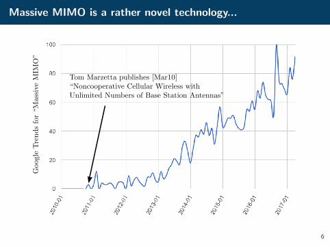
Massive MIMO is a rather novel technology...

6

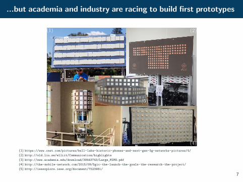
...but academia and industry are racing to build first prototypes

(1) https://www.cnet.com/pictures/bell-labs-historic-phones-and-next-gen-5g-networks-pictures/4/

(2) http://old.liu.se/elliit/Communication/highlights

(3) http://www.academia.edu/download/39443743/Large_MIMO.pdf

(4) http://the-mobile-network.com/2015/09/5gic-the-launch-the-goals-the-research-the-project/

(5) http://ieeexplore.ieee.org/document/7523981/

7

Introduction

Cellular Networks

Basestation

User equipment

Definition (Cellular networks — A major breakthrough)

A cellular network consists of a set of base stations (BSs) and a set of

user equipments (UEs). Each UE is connected to one of the BS, which

provides service to it.

• Downlink (DL) refers to signals sent from the BS to its UEs

• Uplink (UL) refers to signals sent from the UE to its respective BS

8

Area Throughput

Bandwidth(B)

Average cell density (D)

Spectral ef f iciency (SE)

Volume = Area throughput

Definition (Area throughput)

The area throughput of a cellular network is measured in bit/s/km2.

Area throughput = B [Hz] ·D [cells/km2] · SE [bit/s/Hz/cell]

where B is the bandwidth, D is the average cell density, and SE is the

per-cell spectral efficiency (SE). The SE is the amount of information

transferred per second over a unit bandwidth.

9

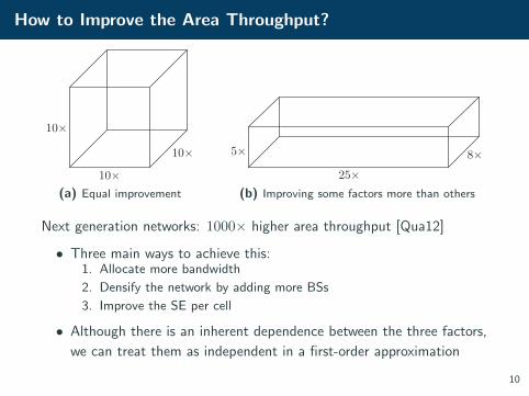
How to Improve the Area Throughput?

10×

10×

10×

(a) Equal improvement

25×8×5×

(b) Improving some factors more than others

Next generation networks: 1000× higher area throughput [Qua12]

• Three main ways to achieve this:1. Allocate more bandwidth

2. Densify the network by adding more BSs

3. Improve the SE per cell

• Although there is an inherent dependence between the three factors,

we can treat them as independent in a first-order approximation

10

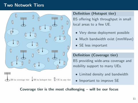
Two Network Tiers

BS in coverage tier BS in hotspot tier UE in any tier

Definition (Hotspot tier)

BS offering high throughput in small

local areas to a few UE.

• Very dense deployment possible

• Much bandwidth exist (mmWave)

• SE less important

Definition (Coverage tier)

BS providing wide-area coverage and

mobility support to many UEs.

• Limited density and bandwidth

• Important to improve SE

Coverage tier is the most challenging – will be our focus

11

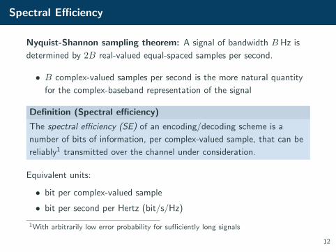
Spectral Efficiency

Nyquist-Shannon sampling theorem: A signal of bandwidth B Hz is

determined by 2B real-valued equal-spaced samples per second.

• B complex-valued samples per second is the more natural quantity

for the complex-baseband representation of the signal

Definition (Spectral efficiency)

The spectral efficiency (SE) of an encoding/decoding scheme is a

number of bits of information, per complex-valued sample, that can be

reliably1 transmitted over the channel under consideration.

Equivalent units:

• bit per complex-valued sample

• bit per second per Hertz (bit/s/Hz)

1With arbitrarily low error probability for sufficiently long signals

12

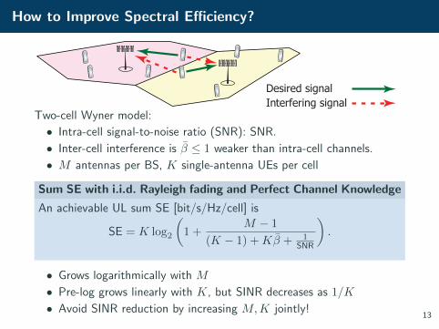
How to Improve Spectral Efficiency?

Desired signalInterfering signal

Two-cell Wyner model:

• Intra-cell signal-to-noise ratio (SNR): SNR.

• Inter-cell interference is β ≤ 1 weaker than intra-cell channels.

• M antennas per BS, K single-antenna UEs per cell

Sum SE with i.i.d. Rayleigh fading and Perfect Channel Knowledge

An achievable UL sum SE [bit/s/Hz/cell] is

SE = K log2

(1 +

M − 1

(K − 1) +Kβ + 1SNR

).

• Grows logarithmically with M

• Pre-log grows linearly with K, but SINR decreases as 1/K

• Avoid SINR reduction by increasing M,K jointly!13

Canonical Definition and

Notation

Canonical Massive MIMO Network

Definition (Canonical Massive MIMO Network)

A canonical Massive MIMO network is a multi-carrier cellular network

with L cells that operate according to a synchronous TDD protocol.2

• BS j is equipped with Mj � 1 antennas, to achieve channel

hardening

• BS j communicates with Kj single-antenna UEs on each

time/frequency sample, where Mj/Kj > 1

• Each BS operates individually and processes its signals using linear

transmit precoding and linear receive combining

2A synchronous TDD protocol refers to a protocol in which UL and DL transmissions

within different cells are synchronized

14

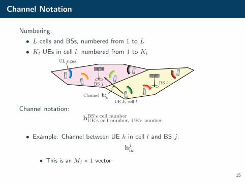
Channel Notation

Numbering:

• L cells and BSs, numbered from 1 to L

• Kl UEs in cell l, numbered from 1 to Kl

BS j

UE k, cell l

hjlk

Channel

BS l

UL signal

Channel notation:

hBS’s cell numberUE’s cell number, UE’s number

• Example: Channel between UE k in cell l and BS j:

hjlk

• This is an Mj × 1 vector

15

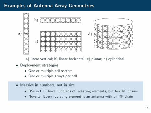
Examples of Antenna Array Geometries

a)

b)

c)

d)

a) linear vertical; b) linear horizontal; c) planar; d) cylindrical.

• Deployment strategies

• One or multiple cell sectors

• One or multiple arrays per cell

• Massive in numbers, not in size

• BSs in LTE have hundreds of radiating elements, but few RF chains

• Novelty: Every radiating element is an antenna with an RF chain

16

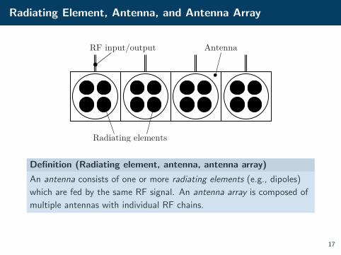
Radiating Element, Antenna, and Antenna Array

Antenna

Radiating elements

RF input/output

Definition (Radiating element, antenna, antenna array)

An antenna consists of one or more radiating elements (e.g., dipoles)

which are fed by the same RF signal. An antenna array is composed of

multiple antennas with individual RF chains.

17

CSI, Coherence block, TDD...

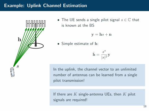
Example: Uplink Channel Estimation

• The UE sends a single pilot signal s ∈ C that

is known at the BS

y = hs+ n

• Simple estimate of h:

h =s?

|s|2 y

In the uplink, the channel vector to an unlimited

number of antennas can be learned from a single

pilot transmission!

If there are K single-antenna UEs, then K pilot

signals are required!

18

Example: Downlink Channel Estimation

• The BS sends a known pilot signal s

subsequently from each antenna

• Received signal at the UE:

ym = hms+ nm m = 1, . . . ,M

• Simple estimate of hm:

hm =s?

|s|2 ym

• The UE feeds h back to the BS3

M pilot transmissions (plus feedback) are needed

to estimate the downlink channel!

3Generally, a quantized version of h is fed back which increases the estimation error.

19

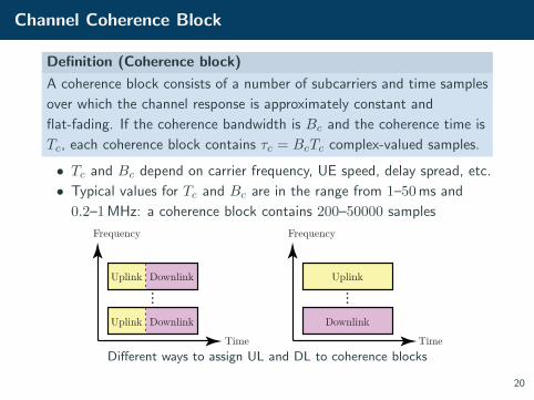
Channel Coherence Block

Definition (Coherence block)

A coherence block consists of a number of subcarriers and time samples

over which the channel response is approximately constant and

flat-fading. If the coherence bandwidth is Bc and the coherence time is

Tc, each coherence block contains τc = BcTc complex-valued samples.

• Tc and Bc depend on carrier frequency, UE speed, delay spread, etc.

• Typical values for Tc and Bc are in the range from 1–50 ms and

0.2–1 MHz: a coherence block contains 200–50000 samples

Time

Frequency

Uplink

Downlink

FDD operation

Frequency

TDD operation

Uplink Downlink

Uplink Downlink

TimeDifferent ways to assign UL and DL to coherence blocks

20

Overhead of CSI Acquisition

Time

Frequency

FDD operation

Frequency

TDD operationTime

M pilots

K pilots + M feedbackK pilots

K pilots

Uplink

Downlink

• Time-division duplex (TDD) — Overhead per block: K pilots

• UL/DL channels are reciprocal

• Only BS needs to know full channels

• Frequency-division duplex (FDD) — Overhead per block: M + K2

• K pilots + M feedback in UL

• M pilots in DL

21

Feasible Operating Points

0 20 40 60 80 1000

10

20

30

40

50

Number of antennas (M)

Num

ber

of U

Es (K

)

FDDTDD

Shaded area: M>4K

Illustration of operating points (M,K) supported by using τp = 20 pilots, for

different TDD and FDD protocols. The shaded area corresponds to operating

points that are preferable in SDMA systems.

Only TDD and the resulting channel reciprocity allow for very large M !

22

Channel Parameterizations

In some propagation scenarios, the M -dimensional channels can be

parameterized using much less than M parameters.

• Key example: LoS propagation

• Mainly depends on the angle between the BS and the UE

• Instead of transmitting M DL pilots, select a set of equally spaced

angles and send precoded DL pilot signals only in these directions

• If the number of angles is much smaller than M , then this method

can enable FDD operation with potentially good estimation quality

But...

• LoS channel parameterizations depends on array geometry

• UE channels are likely a mixture of NLoS and LoS components

TDD operates efficiently in any kind of propagation environment!

23

Spatial Channel Correlation

What is Spatial Channel Correlation?

Definition (Spatial Channel Correlation)

A fading channel h ∈ CM is spatially uncorrelated if the channel gain

‖h‖2 and the channel direction h/‖h‖ are independent random

variables, and the channel direction is uniformly distributed over the

unit-sphere in CM . The channel is otherwise spatially correlated.

Example of uncorrelated channel:

• Uncorrelated Rayleigh fading: h ∼ NC(0, βI)

• All eigenvalues of correlation matrix are equal

Example of correlated channel:

• Any model with eigenvalue variations in the correlation matrix

• Some spatial directions are statistically more likely to contain strong

signal components than others

• Correlated Rayleigh fading: h ∼ NC(0,R)

• More correlation: Larger eigenvalue variations

24

The Correlated Rayleigh Fading Channel Model

Definition (Correlated Rayleigh Fading)

Under the correlated Rayleigh fading channel model, the channel

vectors hjlk ∈ CMj are distributed as hjlk ∼ NC

(0Mj

,Rjlk

), where

Rjlk ∈ CMj×Mj is the spatial channel correlation matrix.

• hjlk takes independent realizations in every coherence block

• Variations in hjlk describe microscopic effects due to movement

• Rjlk is assumed to be known4 at BS j

• The eigenvalues and eigenvectors of Rjlk determine the spatial

channel correlation of hjlk

• Average channel gain is βjlk = 1Mj

tr(Rjlk) per antenna

4Estimation of Rjlk is a very important topic, but will not be covered in this course.

25

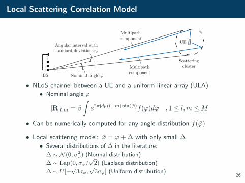
Local Scattering Correlation Model

BS

UE

ScatteringclusterMultipath

component

Multipathcomponent

Nominal angle ϕ

Angular interval withstandard deviation σϕ

. . .

• NLoS channel between a UE and a uniform linear array (ULA)

• Nominal angle ϕ

[R]l,m = β

∫e2πjdH(l−m) sin(ϕ)f(ϕ)dϕ , 1 ≤ l,m ≤M

• Can be numerically computed for any angle distribution f(ϕ)

• Local scattering model: ϕ = ϕ+ ∆ with only small ∆.

• Several distributions of ∆ in the literature:

∆ ∼ N (0, σ2ϕ) (Normal distribution)

∆ ∼ Lap(0, σϕ/√

2) (Laplace distribution)

∆ ∼ U [−√

3σϕ,√

3σϕ] (Uniform distribution)26

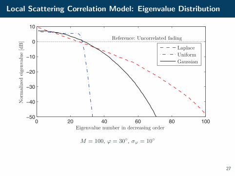
Local Scattering Correlation Model: Eigenvalue Distribution

0 20 40 60 80 100−50

−40

−30

−20

−10

0

10

Eigenvalue number in decreasing order

Nor

mal

ized

eig

enva

lue

[dB]

LaplaceUniformGaussian

Reference: Uncorrelated fading

M = 100, ϕ = 30◦, σϕ = 10◦

27

Channel Hardening and

Favorable Propagation

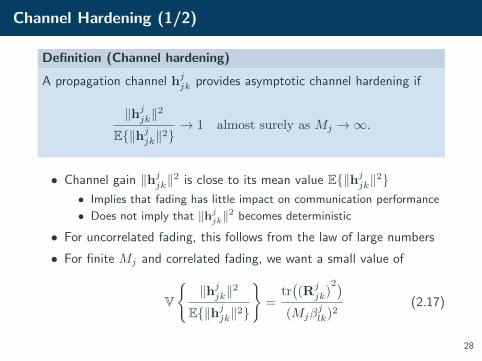
Channel Hardening (1/2)

Definition (Channel hardening)

A propagation channel hjjk provides asymptotic channel hardening if

‖hjjk‖2

E{‖hjjk‖2}→ 1 almost surely as Mj →∞.

• Channel gain ‖hjjk‖2 is close to its mean value E{‖hjjk‖2}• Implies that fading has little impact on communication performance

• Does not imply that ‖hjjk‖2 becomes deterministic

• For uncorrelated fading, this follows from the law of large numbers

• For finite Mj and correlated fading, we want a small value of

V

{‖hjjk‖2

E{‖hjjk‖2}

}=

tr((Rj

jk)2)

(Mjβjlk)2

(2.17)

28

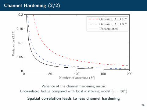
Channel Hardening (2/2)

0 50 100 150 2000

0.05

0.1

0.15

0.2

Number of antennas (M)

Var

ianc

e in

(2.

17)

Gaussian, ASD 10◦

Gaussian, ASD 30◦

Uncorrelated

Variance of the channel hardening metric

Uncorrelated fading compared with local scattering model (ϕ = 30◦)

Spatial correlation leads to less channel hardening

29

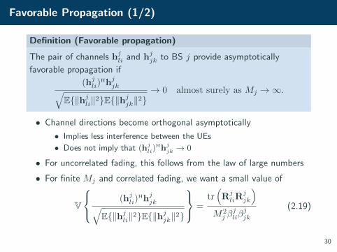
Favorable Propagation (1/2)

Definition (Favorable propagation)

The pair of channels hjli and hjjk to BS j provide asymptotically

favorable propagation if

(hjli)Hhjjk√

E{‖hjli‖2}E{‖hjjk‖2}

→ 0 almost surely as Mj →∞.

• Channel directions become orthogonal asymptotically

• Implies less interference between the UEs

• Does not imply that (hjli)Hhjjk → 0

• For uncorrelated fading, this follows from the law of large numbers

• For finite Mj and correlated fading, we want a small value of

V

(hjli)Hhjjk√

E{‖hjli‖2}E{‖hjjk‖2}

=tr(RjliR

jjk

)M2j β

jliβ

jjk

(2.19)

30

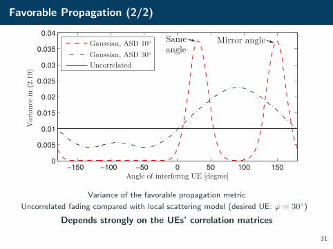
Favorable Propagation (2/2)

−150 −100 −50 0 50 100 1500

0.005

0.01

0.015

0.02

0.025

0.03

0.035

0.04

Angle of interfering UE [degree]

Var

ianc

e in

(2.

19)

Gaussian, ASD 10◦

Gaussian, ASD 30◦

Uncorrelated

Sameangle

Mirror angle

Variance of the favorable propagation metric

Uncorrelated fading compared with local scattering model (desired UE: ϕ = 30◦)

Depends strongly on the UEs’ correlation matrices

31

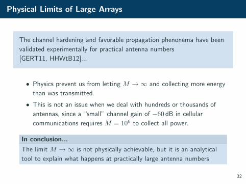
Physical Limits of Large Arrays

The channel hardening and favorable propagation phenonema have been

validated experimentally for practical antenna numbers

[GERT11, HHWtB12]...

• Physics prevent us from letting M →∞ and collecting more energy

than was transmitted.

• This is not an issue when we deal with hundreds or thousands of

antennas, since a “small” channel gain of −60 dB in cellular

communications requires M = 106 to collect all power.

In conclusion...

The limit M →∞ is not physically achievable, but it is an analytical

tool to explain what happens at practically large antenna numbers

32

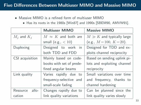
Five Differences Between Multiuser MIMO and Massive MIMO

• Massive MIMO is a refined form of multiuser MIMO

• Has its roots in the 1980s [Win87] and 1990s [SBEM90, AMVW91].

Multiuser MIMO Massive MIMO

Mj and Kj M ≈ K and both are

small (e.g., < 10)

M � K and typically large

(e.g., M=100, K=20).

Duplexing Designed to work in

both TDD and FDD

Designed for TDD and ex-

ploits channel reciprocity

CSI acquisition Mainly based on code-

books with set of prede-

fined angular beams

Based on sending uplink pi-

lots and exploiting channel

reciprocity

Link quality Varies rapidly due to

frequency-selective and

small-scale fading

Small variations over time

and frequency, thanks to

channel hardening

Resource allo-

cation

Changes rapidly due to

link quality variations

Can be planned since the

link quality varies slowly33

Uplink System Model

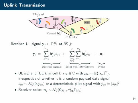
Uplink Transmission

BS j

UE k, cell l

hjlk

Channel

BS l

UL signal

Received UL signal yj ∈ CMj at BS j:

yj =

Kj∑k=1

hjjksjk

︸ ︷︷ ︸Desired signals

+

L∑l=1l6=j

Kl∑i=1

hjlisli

︸ ︷︷ ︸Inter-cell interference

+ nj

︸︷︷︸Noise

• UL signal of UE k in cell l: slk ∈ C with plk = E{|slk|2},irrespective of whether it is a random payload data signal

slk ∼ NC(0, plk) or a deterministic pilot signal with plk = |slk|2

• Receiver noise: nj ∼ NC(0Mj, σ2

ULIMj)

34

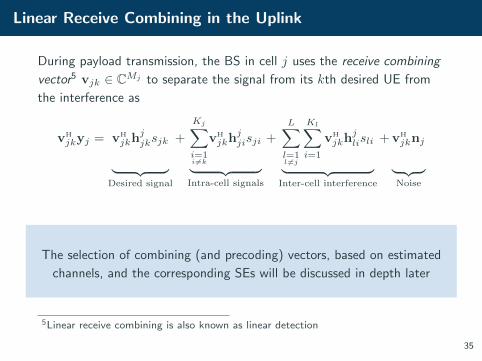
Linear Receive Combining in the Uplink

During payload transmission, the BS in cell j uses the receive combining

vector5 vjk ∈ CMj to separate the signal from its kth desired UE from

the interference as

vH

jkyj = vH

jkhjjksjk

︸ ︷︷ ︸Desired signal

+

Kj∑i=1i6=k

vH

jkhjjisji

︸ ︷︷ ︸Intra-cell signals

+

L∑l=1l 6=j

Kl∑i=1

vH

jkhjlisli

︸ ︷︷ ︸Inter-cell interference

+ vH

jknj

︸ ︷︷ ︸Noise

The selection of combining (and precoding) vectors, based on estimated

channels, and the corresponding SEs will be discussed in depth later

5Linear receive combining is also known as linear detection

35

Received Uplink Signal During Pilot Transmission

Bc

Coherence time Tc

Coherencebandwidth

τp

τu τdUL data DL data

UL pilots:

Received UL signal Ypj ∈ CMj×τp at BS j:

Ypj =

Kj∑k=1

√pjkh

jjkφ

T

jk

︸ ︷︷ ︸Desired pilots

+

L∑l=1l 6=j

Kl∑i=1

√plih

jliφ

T

li

︸ ︷︷ ︸Inter-cell pilots

+ Npj

︸︷︷︸Noise

• UE k in cell j transmits the pilot sequence φjk ∈ Cτp

• ‖φjk‖2 = φH

jkφjk = τp (scaled by UE’s transmit power as√pjk)

• Npj ∈ CMj×τp has i.i.d. NC(0, σ2

UL) elements

36

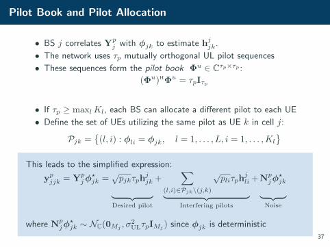
Pilot Book and Pilot Allocation

• BS j correlates Ypj with φjk to estimate hjjk.

• The network uses τp mutually orthogonal UL pilot sequences

• These sequences form the pilot book Φu ∈ Cτp×τp :

(Φu)HΦu = τpIτp

• If τp ≥ maxlKl, each BS can allocate a different pilot to each UE

• Define the set of UEs utilizing the same pilot as UE k in cell j:

Pjk ={

(l, i) : φli = φjk, l = 1, . . . , L, i = 1, . . . ,Kl

}This leads to the simplified expression:

ypjjk = Ypjφ

?jk =

√pjkτph

jjk︸ ︷︷ ︸

Desired pilot

+∑

(l,i)∈Pjk\(j,k)

√pliτph

jli︸ ︷︷ ︸

Interfering pilots

+ Npjφ

?jk︸ ︷︷ ︸

Noise

where Npjφ

?jk ∼ NC(0Mj , σ

2ULτpIMj ) since φjk is deterministic

37

MMSE Channel Estimation

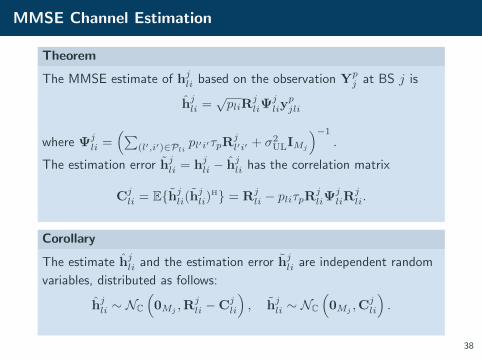
MMSE Channel Estimation

Theorem

The MMSE estimate of hjli based on the observation Ypj at BS j is

hjli =√pliR

jliΨ

jliy

pjli

where Ψjli =

(∑(l′,i′)∈Pli

pl′i′τpRjl′i′ + σ2

ULIMj

)−1

.

The estimation error hjli = hjli − hjli has the correlation matrix

Cjli = E{hjli(h

jli)

H} = Rjli − pliτpR

jliΨ

jliR

jli.

Corollary

The estimate hjli and the estimation error hjli are independent random

variables, distributed as follows:

hjli ∼ NC

(0Mj ,R

jli −Cj

li

), hjli ∼ NC

(0Mj ,C

jli

).

38

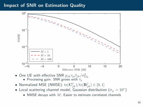
Impact of SNR on Estimation Quality

−10 −5 0 5 10 15 2010−3

10−2

10−1

100

Ef fective SNR [dB]

NM

SE

M = 1M = 10M = 100

• One UE with effective SNR pjkτpβjk/σ2UL

• Processing gain: SNR grows with τp

• Normalized MSE (NMSE): tr(Cjjk)/tr(Rj

jk) ∈ [0, 1]

• Local scattering channel model, Gaussian distribution (σϕ = 10◦)

• NMSE decays with M : Easier to estimate correlated channels

39

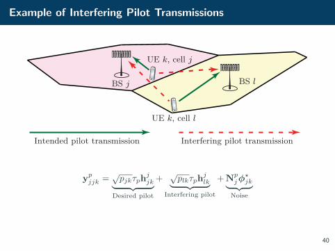
Example of Interfering Pilot Transmissions

BS j

UE k, cell l

BS l

UE k, cell j

Intended pilot transmission Interfering pilot transmission

ypjjk =√pjkτph

jjk︸ ︷︷ ︸

Desired pilot

+√plkτph

jlk︸ ︷︷ ︸

Interfering pilot

+ Npjφ

?jk︸ ︷︷ ︸

Noise

40

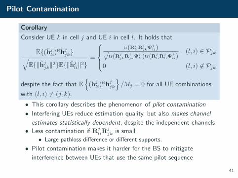
Pilot Contamination

Corollary

Consider UE k in cell j and UE i in cell l. It holds that

E{(hjli)Hhjjk}√E{‖hjjk‖2}E{‖h

jli‖2}

=

tr(Rj

liRjjkΨj

li)√tr(Rj

jkRjjkΨj

li)tr(RjliR

jliΨ

jli)

(l, i) ∈ Pjk

0 (l, i) 6∈ Pjk

despite the fact that E{

(hjli)Hhjjk

}/Mj = 0 for all UE combinations

with (l, i) 6= (j, k).

• This corollary describes the phenomenon of pilot contamination

• Interfering UEs reduce estimation quality, but also makes channel

estimates statistically dependent, despite the independent channels

• Less contamination if RjliR

jjk is small

• Large pathloss difference or different supports.

• Pilot contamination makes it harder for the BS to mitigate

interference between UEs that use the same pilot sequence

41

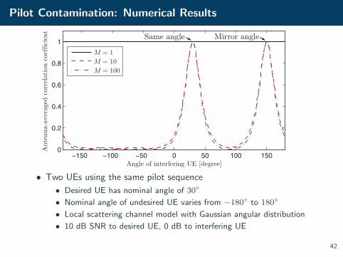
Pilot Contamination: Numerical Results

−150 −100 −50 0 50 100 1500

0.2

0.4

0.6

0.8

1

Angle of interfering UE [degree]

Ant

enna

-ave

rage

d co

rrel

atio

n co

ef f ic

ient

M = 1M = 10M = 100

Same angle Mirror angle

• Two UEs using the same pilot sequence

• Desired UE has nominal angle of 30◦

• Nominal angle of undesired UE varies from −180◦ to 180◦

• Local scattering channel model with Gaussian angular distribution

• 10 dB SNR to desired UE, 0 dB to interfering UE

42

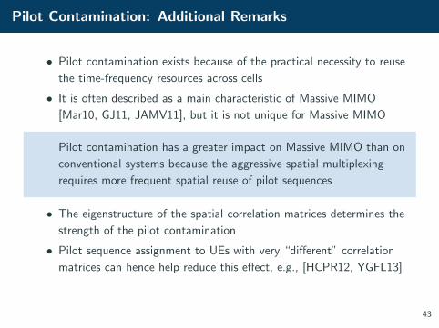
Pilot Contamination: Additional Remarks

• Pilot contamination exists because of the practical necessity to reuse

the time-frequency resources across cells

• It is often described as a main characteristic of Massive MIMO

[Mar10, GJ11, JAMV11], but it is not unique for Massive MIMO

Pilot contamination has a greater impact on Massive MIMO than on

conventional systems because the aggressive spatial multiplexing

requires more frequent spatial reuse of pilot sequences

• The eigenstructure of the spatial correlation matrices determines the

strength of the pilot contamination

• Pilot sequence assignment to UEs with very “different” correlation

matrices can hence help reduce this effect, e.g., [HCPR12, YGFL13]

43

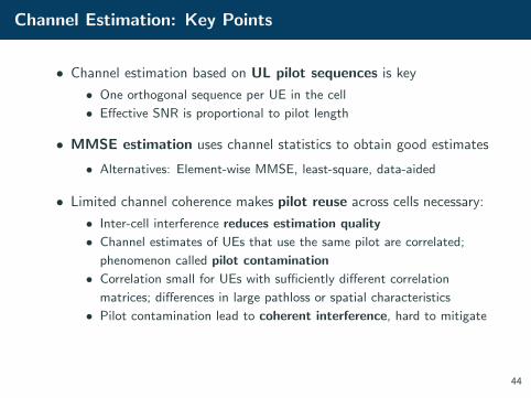
Channel Estimation: Key Points

• Channel estimation based on UL pilot sequences is key

• One orthogonal sequence per UE in the cell

• Effective SNR is proportional to pilot length

• MMSE estimation uses channel statistics to obtain good estimates

• Alternatives: Element-wise MMSE, least-square, data-aided

• Limited channel coherence makes pilot reuse across cells necessary:

• Inter-cell interference reduces estimation quality

• Channel estimates of UEs that use the same pilot are correlated;

phenomenon called pilot contamination

• Correlation small for UEs with sufficiently different correlation

matrices; differences in large pathloss or spatial characteristics

• Pilot contamination lead to coherent interference, hard to mitigate

44

Uplink Spectral Efficiency

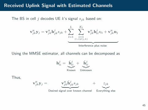
Received Uplink Signal with Estimated Channels

The BS in cell j decodes UE k’s signal sjk based on:

vH

jkyj = vH

jkhjjksjk +

L∑l=1

Kl∑i=1

(l,i)6=(j,k)

vH

jkhjlisli + vH

jknj

︸ ︷︷ ︸Interference plus noise

Using the MMSE estimator, all channels can be decomposed as

hjli = hjli︸︷︷︸Known

+ hjli︸︷︷︸Unknown

Thus,

vH

jkyj = vH

jkhjjksjk︸ ︷︷ ︸

Desired signal over known channel

+ zjk︸︷︷︸Everything else

45

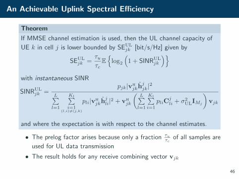
An Achievable Uplink Spectral Efficiency

Theorem

If MMSE channel estimation is used, then the UL channel capacity of

UE k in cell j is lower bounded by SEULjk [bit/s/Hz] given by

SEULjk =

τuτc

E{

log2

(1 + SINRUL

jk

)}with instantaneous SINR

SINRULjk =

pjk|vH

jkhjjk|2

L∑l=1

Kl∑i=1

(l,i) 6=(j,k)

pli|vH

jkhjli|2 + vH

jk

(L∑l=1

Kl∑i=1

pliCjli + σ2

ULIMj

)vjk

and where the expectation is with respect to the channel estimates.

• The prelog factor arises because only a fraction τuτc

of all samples are

used for UL data transmission

• The result holds for any receive combining vector vjk

46

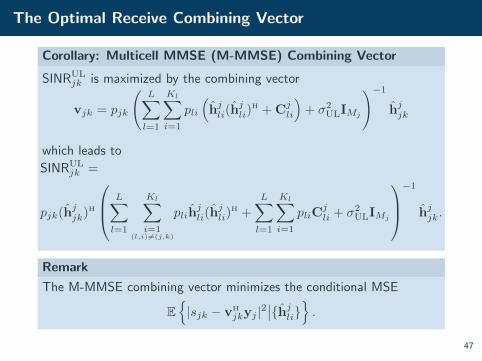
The Optimal Receive Combining Vector

Corollary: Multicell MMSE (M-MMSE) Combining Vector

SINRULjk is maximized by the combining vector

vjk = pjk

(L∑l=1

Kl∑i=1

pli

(hjli(h

jli)

H + Cjli

)+ σ2

ULIMj

)−1

hjjk

which leads to

SINRULjk =

pjk(hjjk)H

L∑l=1

Kl∑i=1

(l,i)6=(j,k)

plihjli(h

jli)

H +

L∑l=1

Kl∑i=1

pliCjli + σ2

ULIMj

−1

hjjk.

Remark

The M-MMSE combining vector minimizes the conditional MSE

E{|sjk − vH

jkyj |2∣∣{hjli}} .

47

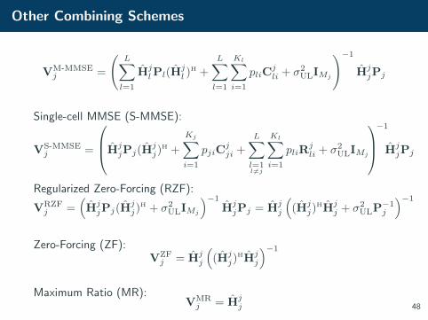
Other Combining Schemes

VM-MMSEj =

(L∑l=1

HjlPl(H

jl )

H +

L∑l=1

Kl∑i=1

pliCjli + σ2

ULIMj

)−1

HjjPj

Single-cell MMSE (S-MMSE):

VS-MMSEj =

HjjPj(H

jj)

H +

Kj∑i=1

pjiCjji +

L∑l=1l6=j

Kl∑i=1

pliRjli + σ2

ULIMj

−1

HjjPj

Regularized Zero-Forcing (RZF):

VRZFj =

(HjjPj(H

jj)

H + σ2ULIMj

)−1

HjjPj = Hj

j

((Hj

j)HHj

j + σ2ULP−1

j

)−1

Zero-Forcing (ZF):VZFj = Hj

j

((Hj

j)HHj

j

)−1

Maximum Ratio (MR):VMRj = Hj

j 48

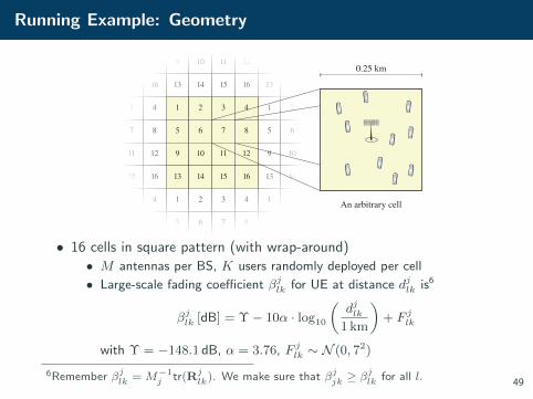
Running Example: Geometry

9 10 11 12

13 14 15 16

1 2

5 6

9 10

13 14

9 10

13 14

3 4

7 8

11 12

15 16

11 12

15 16

1 2

5 6

1 2 3 4

5 6 7 8

3 4

7 8

An arbitrary cell

0.25 km

1 2 3 4

5 6 7 8

9 10 11 12

13 14 15 16

• 16 cells in square pattern (with wrap-around)

• M antennas per BS, K users randomly deployed per cell

• Large-scale fading coefficient βjlk for UE at distance djlk is6

βjlk [dB] = Υ− 10α · log10

(djlk

1 km

)+ F jlk

with Υ = −148.1 dB, α = 3.76, F jlk ∼ N (0, 72)

6Remember βjlk =M−1j tr(Rj

lk). We make sure that βjjk ≥ βjlk for all l.

49

Running Example: Power and Pilot Reuse

• Bandwidth B = 20 MHz

• UL/DL transmit power: 20 dBm per UE

• Total noise power: −94 dBm

• SNR: 20.5 dB (cell center), −5.8 dB (cell corner), before shadowing

• Comparison of channel models

• Gaussian local scattering: ASD σϕ

• Uncorrelated Rayleigh fading: Rjlk = βjlkIM

• Pilot reuse factor f ∈ {1, 2, 4}• τp = fK UL pilot sequences

• K pilot sequences per cell, reused in 1/f of the cells

2 4

5 7

10 12

13 15

1 2 3 4

5 6 7 8

9 10 11 12

13 14 15 16

Pilot reuse f=1 Pilot reuse f=2 Pilot reuse f=4

1 3

6 8

9 11

14 16

1 2 3 4

5 6 7 8

9 10 11 12

13 14 15 16

50

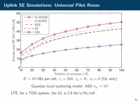
Uplink SE Simulations: Universal Pilot Reuse

10 20 30 40 50 60 70 80 90 1000

10

20

30

40

50

60

Number of antennas (M)

Ave

rage

sum

SE

[bit/

s/H

z/ce

ll]

M-MMSES-MMSERZFZFMR

K = 10 UEs per cell, τc = 200, τp = K, τd = 0 (UL only)

Gaussian local scattering model: ASD σϕ = 10◦

LTE: for a TDD system, the UL is 2.8 bit/s/Hz/cell

51

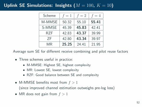
Uplink SE Simulations: Insights (M = 100, K = 10)

Scheme f = 1 f = 2 f = 4

M-MMSE 50.32 55.10 55.41

S-MMSE 45.39 45.83 42.41

RZF 42.83 43.37 39.99

ZF 42.80 43.34 39.97

MR 25.25 24.41 21.95

Average sum SE for different receive combining and pilot reuse factors

• Three schemes useful in practice:

• M-MMSE: Highest SE, highest complexity

• MR: Lowest SE, lowest complexity

• RZF: Good balance between SE and complexity

• M-MMSE benefits most from f > 1

(since improved channel estimation outweighs pre-log loss)

• MR does not gain from f > 1

52

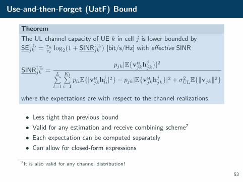
Use-and-then-Forget (UatF) Bound

Theorem

The UL channel capacity of UE k in cell j is lower bounded by

SEULjk = τu

τclog2(1 + SINRUL

jk ) [bit/s/Hz] with effective SINR

SINRULjk =

pjk|E{vH

jkhjjk}|2

L∑l=1

Kl∑i=1

pliE{|vH

jkhjli|2} − pjk|E{vH

jkhjjk}|2 + σ2

ULE{‖vjk‖2}

where the expectations are with respect to the channel realizations.

• Less tight than previous bound

• Valid for any estimation and receive combining scheme7

• Each expectation can be computed separately

• Can allow for closed-form expressions

7It is also valid for any channel distribution!

53

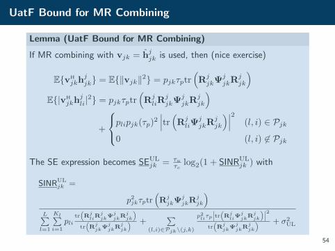
UatF Bound for MR Combining

Lemma (UatF Bound for MR Combining)

If MR combining with vjk = hjjk is used, then (nice exercise)

E{vH

jkhjjk} = E{‖vjk‖2} = pjkτptr

(RjjkΨ

jjkR

jjk

)E{|vH

jkhjli|2} = pjkτptr

(RjliR

jjkΨ

jjkR

jjk

)+

plipjk(τp)2∣∣∣tr(Rj

liΨjjkR

jjk

)∣∣∣2 (l, i) ∈ Pjk0 (l, i) 6∈ Pjk

The SE expression becomes SEULjk = τu

τclog2(1 + SINRUL

jk ) with

SINRULjk =

p2jkτptr(RjjkΨ

jjkR

jjk

)L∑l=1

Kl∑i=1

plitr(R

jli

Rjjk

Ψjjk

Rjjk

)tr(R

jjk

Ψjjk

Rjjk

) +∑

(l,i)∈Pjk\(j,k)

p2liτp

∣∣∣tr(Rjli

Ψjjk

Rjjk

)∣∣∣2tr(R

jjk

Ψjjk

Rjjk

) + σ2UL

54

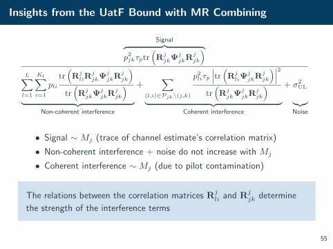
Insights from the UatF Bound with MR Combining

Signal︷ ︸︸ ︷p2jkτptr

(RjjkΨ

jjkR

jjk

)L∑l=1

Kl∑i=1

plitr(RjliR

jjkΨ

jjkR

jjk

)tr(RjjkΨ

jjkR

jjk

)︸ ︷︷ ︸

Non-coherent interference

+∑

(l,i)∈Pjk\(j,k)

p2liτp

∣∣∣tr(RjliΨ

jjkR

jjk

)∣∣∣2tr(RjjkΨ

jjkR

jjk

)︸ ︷︷ ︸

Coherent interference

+ σ2UL

︸︷︷︸Noise

• Signal ∼Mj (trace of channel estimate’s correlation matrix)

• Non-coherent interference + noise do not increase with Mj

• Coherent interference ∼Mj (due to pilot contamination)

The relations between the correlation matrices Rjli and Rj

jk determine

the strength of the interference terms

55

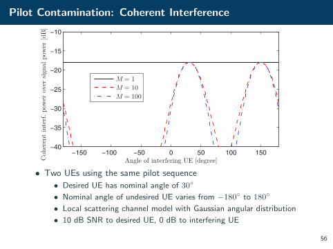
Pilot Contamination: Coherent Interference

−150 −100 −50 0 50 100 150−40

−35

−30

−25

−20

−15

−10

Angle of interfering UE [degree]Coh

eren

t in

terf.

pow

er o

ver

signa

l pow

er [d

B]

M = 1M = 10M = 100

• Two UEs using the same pilot sequence

• Desired UE has nominal angle of 30◦

• Nominal angle of undesired UE varies from −180◦ to 180◦

• Local scattering channel model with Gaussian angular distribution

• 10 dB SNR to desired UE, 0 dB to interfering UE

56

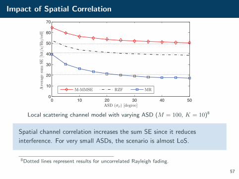
Impact of Spatial Correlation

0 10 20 30 40 500

10

20

30

40

50

60

70

ASD (σϕ) [degree]

Ave

rage

sum

SE

[bit/

s/H

z/ce

ll]

M-MMSE RZF MR

Local scattering channel model with varying ASD (M = 100, K = 10)8

Spatial channel correlation increases the sum SE since it reduces

interference. For very small ASDs, the scenario is almost LoS.

8Dotted lines represent results for uncorrelated Rayleigh fading.

57

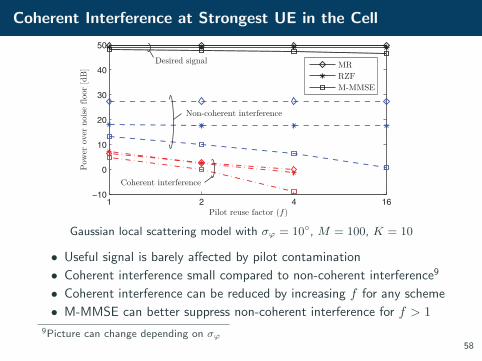
Coherent Interference at Strongest UE in the Cell

1 2 4 16−10

0

10

20

30

40

50

Pilot reuse factor (f)

Pow

er o

ver

noise

f loo

r [d

B]

MRRZFM-MMSE

Desired signal

Non-coherent interference

Coherent interference

Gaussian local scattering model with σϕ = 10◦, M = 100, K = 10

• Useful signal is barely affected by pilot contamination

• Coherent interference small compared to non-coherent interference9

• Coherent interference can be reduced by increasing f for any scheme

• M-MMSE can better suppress non-coherent interference for f > 1

9Picture can change depending on σϕ58

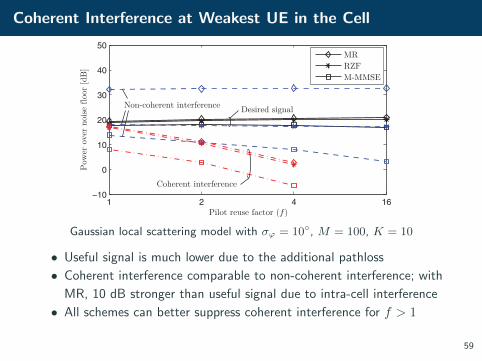
Coherent Interference at Weakest UE in the Cell

1 2 4 16−10

0

10

20

30

40

50

Pilot reuse factor (f)

Pow

er o

ver

noise

f loo

r [d

B]

MRRZFM-MMSE

Desired signalNon-coherent interference

Coherent interference

Gaussian local scattering model with σϕ = 10◦, M = 100, K = 10

• Useful signal is much lower due to the additional pathloss

• Coherent interference comparable to non-coherent interference; with

MR, 10 dB stronger than useful signal due to intra-cell interference

• All schemes can better suppress coherent interference for f > 1

59

Uplink Spectral Efficiency: Key Points

• Lower bound on UL capacity based on MMSE channel estimation

• An achievable SE, maximized by M-MMSE combining

• Combining schemes: M-MMSE, S-MMSE, RZF, ZF, MR

• Factors that affect SE

• Transmit powers

• Pilot reuse factor

• Spatial channel correlation

• Pilot contamination

• Insights from SE analysis and running example

• Received signal power and coherent interference linear in M

• Non-coherent interference and noise independent of M

• Coherent interference negligible for large pilot reuse factors

• UatF bound based on “average” channel:

• Gives closed-form SE expressions with MR

• Only tight with significant channel hardening

60

Downlink Spectral Efficiency

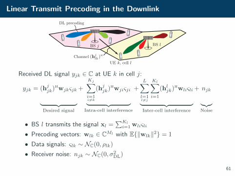
Linear Transmit Precoding in the Downlink

BS j

UE k, cell l

Channel

BS l

DL precoding

(hjlk )H

Received DL signal yjk ∈ C at UE k in cell j:

yjk = (hjjk)Hwjkςjk

︸ ︷︷ ︸Desired signal

+

Kj∑i=1i6=k

(hjjk)Hwjiςji

︸ ︷︷ ︸Intra-cell interference

+

L∑l=1l 6=j

Kl∑i=1

(hljk)Hwliςli

︸ ︷︷ ︸Inter-cell interference

+ njk

︸︷︷︸Noise

• BS l transmits the signal xl =∑Kl

i=1 wliςli

• Precoding vectors: wlk ∈ CMl with E{‖wlk‖2} = 1

• Data signals: ςlk ∼ NC(0, ρlk)

• Receiver noise: njk ∼ NC(0, σ2DL)

61

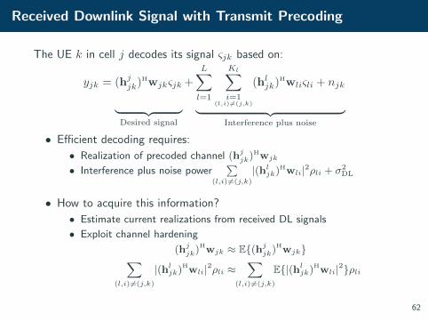
Received Downlink Signal with Transmit Precoding

The UE k in cell j decodes its signal ςjk based on:

yjk = (hjjk)Hwjkςjk

︸ ︷︷ ︸Desired signal

+

L∑l=1

Kl∑i=1

(l,i)6=(j,k)

(hljk)Hwliςli + njk

︸ ︷︷ ︸Interference plus noise

• Efficient decoding requires:

• Realization of precoded channel (hjjk)Hwjk

• Interference plus noise power∑

(l,i)6=(j,k)

|(hljk)Hwli|2ρli + σ2DL

• How to acquire this information?

• Estimate current realizations from received DL signals

• Exploit channel hardening

(hjjk)Hwjk ≈ E{(hjjk)Hwjk}∑(l,i)6=(j,k)

|(hljk)Hwli|2ρli ≈∑

(l,i)6=(j,k)

E{|(hljk)Hwli|2}ρli

62

A Downlink Spectral Efficiency (Hardening Bound)

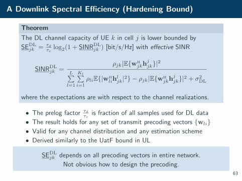
Theorem

The DL channel capacity of UE k in cell j is lower bounded by

SEDLjk = τd

τclog2(1 + SINRDL

jk ) [bit/s/Hz] with effective SINR

SINRDLjk =

ρjk|E{wH

jkhjjk}|2

L∑l=1

Kl∑i=1

ρliE{|wH

lihljk|2} − ρjk|E{wH

jkhjjk}|2 + σ2

DL

where the expectations are with respect to the channel realizations.

• The prelog factor τdτc

is fraction of all samples used for DL data

• The result holds for any set of transmit precoding vectors {wli}• Valid for any channel distribution and any estimation scheme

• Derived similarly to the UatF bound in UL

SEDLjk depends on all precoding vectors in entire network.

Not obvious how to design the precoding.63

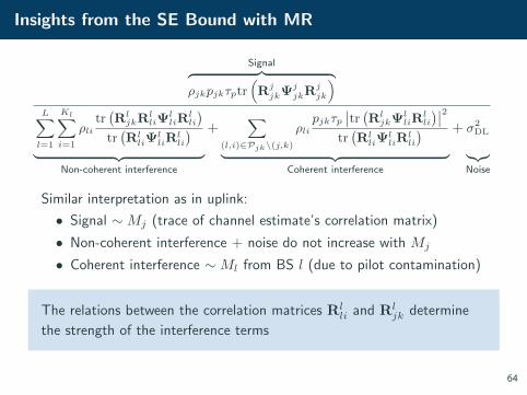
Insights from the SE Bound with MR

Signal︷ ︸︸ ︷ρjkpjkτptr

(RjjkΨ

jjkR

jjk

)L∑l=1

Kl∑i=1

ρlitr(RljkR

lliΨ

lliR

lli

)tr(RlliΨ

lliR

lli

)︸ ︷︷ ︸

Non-coherent interference

+∑

(l,i)∈Pjk\(j,k)

ρlipjkτp

∣∣tr (RljkΨ

lliR

lli

)∣∣2tr(RlliΨ

lliR

lli

)︸ ︷︷ ︸

Coherent interference

+ σ2DL

︸︷︷︸Noise

Similar interpretation as in uplink:

• Signal ∼Mj (trace of channel estimate’s correlation matrix)

• Non-coherent interference + noise do not increase with Mj

• Coherent interference ∼Ml from BS l (due to pilot contamination)

The relations between the correlation matrices Rlli and Rl

jk determine

the strength of the interference terms

64

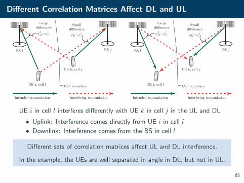
Different Correlation Matrices Affect DL and UL

BS jBS l

UE k, cell j

UE i, cell l

ϕ ljk ϕ l

li– ϕj

li ϕjjk

–

Largedifference

Smalldifference

Cell boundary

Intended transmission Interfering transmission

BS jBS l

UE k, cell j

UE i, cell l

ϕ ljk ϕ l

li– ϕj

li ϕjjk

–

Largedifference

Smalldifference

Cell boundary

Intended transmission Interfering transmission

UE i in cell l interferes differently with UE k in cell j in the UL and DL

• Uplink: Interference comes directly from UE i in cell l

• Downlink: Interference comes from the BS in cell l

Different sets of correlation matrices affect UL and DL interference.

In the example, the UEs are well separated in angle in DL, but not in UL.

65

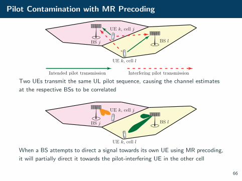
Pilot Contamination with MR Precoding

BS j

UE k, cell l

BS l

UE k, cell j

Intended pilot transmission Interfering pilot transmission

Two UEs transmit the same UL pilot sequence, causing the channel estimates

at the respective BSs to be correlated

BS j

UE k, cell l

BS l

UE k, cell j

When a BS attempts to direct a signal towards its own UE using MR precoding,

it will partially direct it towards the pilot-interfering UE in the other cell

66

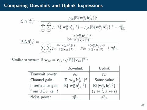
Comparing Downlink and Uplink Expressions

SINRDLjk =

ρjk|E{wH

jkhjjk}|2

L∑l=1

Kl∑i=1

ρliE{|wH

lihljk|2} − ρjk|E{wH

jkhjjk}|2 + σ2

DL

SINRULjk =

pjk|E{vH

jkhjjk}|

2

E{‖vjk‖2}L∑l=1

Kl∑i=1

pliE{|vH

jkhjli|2}

E{‖vjk‖2} − pjk|E{vH

jkhjjk}|2

E{‖vjk‖2} + σ2UL

Similar structure if wjk = vjk/√E{‖vjk‖2}:

Downlink Uplink

Transmit power ρli pli

Channel gain |E{wH

jkhjjk}|2 Same value

Interference gain E{|wH

lihljk|2} E{|wH

jkhjli|2}

from UE i, cell l (j ↔ l, k ↔ i)

Noise power σ2DL σ2

UL

67

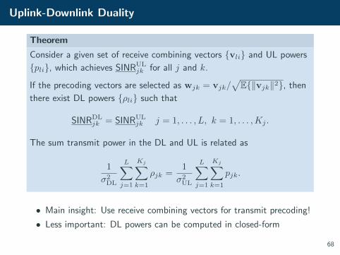
Uplink-Downlink Duality

Theorem

Consider a given set of receive combining vectors {vli} and UL powers

{pli}, which achieves SINRULjk for all j and k.

If the precoding vectors are selected as wjk = vjk/√E{‖vjk‖2}, then

there exist DL powers {ρli} such that

SINRDLjk = SINRUL

jk j = 1, . . . , L, k = 1, . . . ,Kj .

The sum transmit power in the DL and UL is related as

1

σ2DL

L∑j=1

Kj∑k=1

ρjk =1

σ2UL

L∑j=1

Kj∑k=1

pjk.

• Main insight: Use receive combining vectors for transmit precoding!

• Less important: DL powers can be computed in closed-form

68

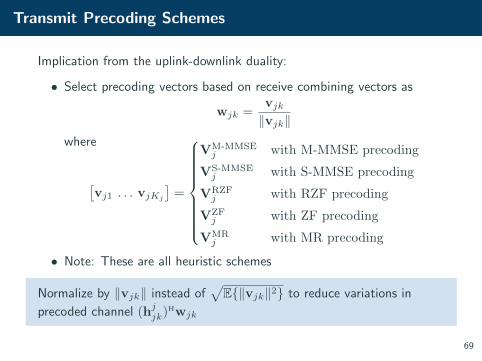
Transmit Precoding Schemes

Implication from the uplink-downlink duality:

• Select precoding vectors based on receive combining vectors as

wjk =vjk‖vjk‖

where

[vj1 . . . vjKj

]=

VM-MMSEj with M-MMSE precoding

VS-MMSEj with S-MMSE precoding

VRZFj with RZF precoding

VZFj with ZF precoding

VMRj with MR precoding

• Note: These are all heuristic schemes

Normalize by ‖vjk‖ instead of√

E{‖vjk‖2} to reduce variations in

precoded channel (hjjk)Hwjk

69

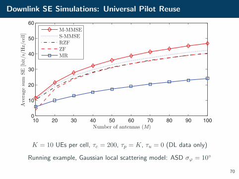
Downlink SE Simulations: Universal Pilot Reuse

10 20 30 40 50 60 70 80 90 1000

10

20

30

40

50

60

Number of antennas (M)

Ave

rage

sum

SE

[bit/

s/H

z/ce

ll]

M-MMSES-MMSERZFZFMR

K = 10 UEs per cell, τc = 200, τp = K, τu = 0 (DL data only)

Running example, Gaussian local scattering model: ASD σϕ = 10◦

70

Asymptotic Analysis

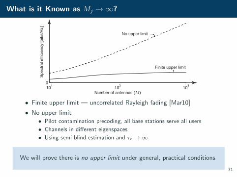
What is it Known as Mj →∞?

101 102 1030

Number of antennas (M)

Spec

tral e

ffici

ency

[bit/

s/H

z]

Finite upper limit

No upper limit

• Finite upper limit — uncorrelated Rayleigh fading [Mar10]

• No upper limit

• Pilot contamination precoding, all base stations serve all users

• Channels in different eigenspaces

• Using semi-blind estimation and τc →∞

We will prove there is no upper limit under general, practical conditions

71

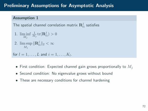
Preliminary Assumptions for Asymptotic Analysis

Assumption 1

The spatial channel correlation matrix Rjli satisfies

1. lim infMj

1Mj

tr(Rjli) > 0

2. lim supMj

‖Rjli‖2 <∞

for l = 1, . . . , L and i = 1, . . . ,Kl.

• First condition: Expected channel gain grows proportionally to Mj

• Second condition: No eigenvalue grows without bound

• These are necessary conditions for channel hardening

72

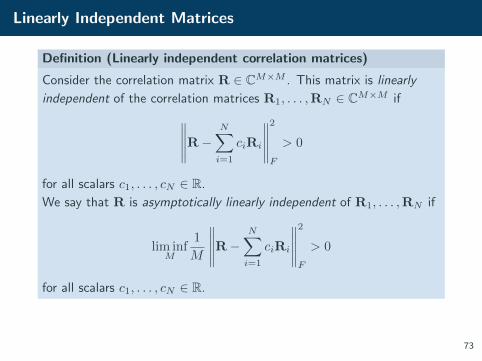
Linearly Independent Matrices

Definition (Linearly independent correlation matrices)

Consider the correlation matrix R ∈ CM×M . This matrix is linearly

independent of the correlation matrices R1, . . . ,RN ∈ CM×M if∥∥∥∥∥R−N∑i=1

ciRi

∥∥∥∥∥2

F

> 0

for all scalars c1, . . . , cN ∈ R.

We say that R is asymptotically linearly independent of R1, . . . ,RN if

lim infM

1

M

∥∥∥∥∥R−N∑i=1

ciRi

∥∥∥∥∥2

F

> 0

for all scalars c1, . . . , cN ∈ R.

73

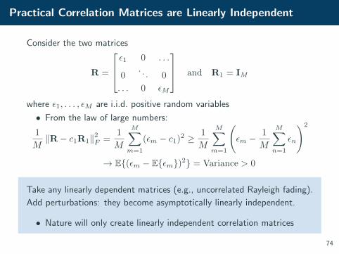
Practical Correlation Matrices are Linearly Independent

Consider the two matrices

R =

ε1 0 . . .

0. . . 0

. . . 0 εM

and R1 = IM

where ε1, . . . , εM are i.i.d. positive random variables

• From the law of large numbers:

1

M‖R− c1R1‖2F =

1

M

M∑m=1

(εm − c1)2 ≥ 1

M

M∑m=1

(εm −

1

M

M∑n=1

εn

)2

→ E{(εm − E{εm})2} = Variance > 0

Take any linearly dependent matrices (e.g., uncorrelated Rayleigh fading).

Add perturbations: they become asymptotically linearly independent.

• Nature will only create linearly independent correlation matrices

74

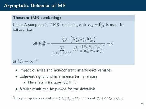
Asymptotic Behavior of MR

Theorem (MR combining)

Under Assumption 1, if MR combining with vjk = hjjk is used, it

follows that

SINRULjk −

p2jktr

(RjjkΨ

jjkR

jjk

)∑

(l,i)∈Pjk\(j,k)

p2li

|tr(RjliΨ

jjkRj

jk)|2tr(Rj

jkΨjjkRj

jk)

→ 0

as Mj →∞.10

• Impact of noise and non-coherent interference vanishes

• Coherent signal and interference terms remain

• There is a finite upper SE limit

• Similar result can be proved for the downlink

10Except in special cases when tr(RjjkR

jli)/Mj → 0 for all (l, i) ∈ Pjk \ (j, k)

75

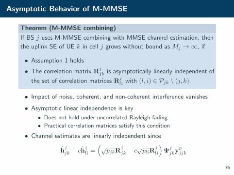
Asymptotic Behavior of M-MMSE

Theorem (M-MMSE combining)

If BS j uses M-MMSE combining with MMSE channel estimation, then

the uplink SE of UE k in cell j grows without bound as Mj →∞, if

• Assumption 1 holds

• The correlation matrix Rjjk is asymptotically linearly independent of

the set of correlation matrices Rjli with (l, i) ∈ Pjk \ (j, k).

• Impact of noise, coherent, and non-coherent interference vanishes

• Asymptotic linear independence is key

• Does not hold under uncorrelated Rayleigh fading

• Practical correlation matrices satisfy this condition

• Channel estimates are linearly independent since

hjjk − chjli =

(√pjkR

jjk − c

√pliR

jli

)Ψjjky

pjjk

76

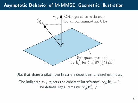
Asymptotic Behavior of M-MMSE: Geometric Illustration

Subspace spanned by for hj

li (l,i)∈Pujk

\(j,k)

hjjk

vjk Orthogonal to estimates for all contaminating UEs

UEs that share a pilot have linearly independent channel estimates

The indicated vjk rejects the coherent interference: vH

jkhjli = 0

The desired signal remains: vH

jkhjjk 6= 0

77

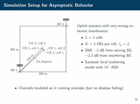
Simulation Setup for Asymptotic Behavior

200 m

200 m

3.6 degrees140 m

UE 1, cell 1UE 2, cell 1

BS 1

BS 2

UE 2, cell 2UE 1, cell 2

Uplink scenario with very strong co-

herent interference:

• L = 2 cells

• K = 2 UEs per cell, τp = 2.

• SNR −2 dB from serving BS,

−2.3 dB from interfering BS

• Gaussian local scattering

model with 10◦ ASD

• Channels modeled as in running example (but no shadow fading)

78

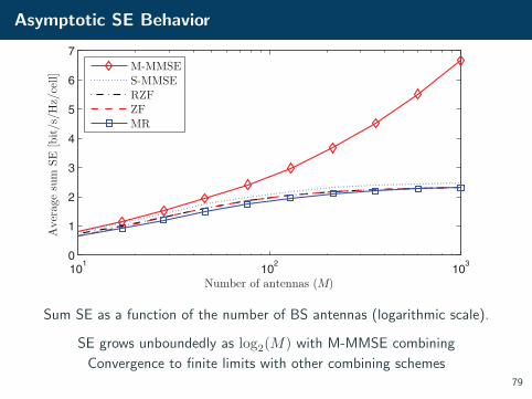
Asymptotic SE Behavior

101

102

103

0

1

2

3

4

5

6

7

Number of antennas (M)

Ave

rage

sum

SE

[bit/

s/H

z/ce

ll]

M-MMSES-MMSERZFZFMR

Sum SE as a function of the number of BS antennas (logarithmic scale).

SE grows unboundedly as log2(M) with M-MMSE combining

Convergence to finite limits with other combining schemes79

Is Pilot Contamination a Fundamental Limitation?

101 102 1030

Number of antennas (M)

Spec

tral e

ffici

ency

[bit/

s/H

z]

Finite upper limit

No contamination: No asymptotic limit

Pilot contamination:No asymptotic limit

No! Unlimited capacity is achieved using the following ingredients

• Spatial correlated channels – only a minor amount is needed

• MMSE channel estimation – not least-square

• Optimal linear combining – not MR, ZF, or S-MMSE80

Key Points

• Asymptotic behavior

• Impact of noise and non-coherent interference always vanish

• Coherent interference caused by pilot contamination is a challenge

• Impact of coherent interference vanish with M-MMSE

• SE grows as log2(M) when using M-MMSE

• Spatial channel correlation is important in asymptotic analysis

• Enables unbounded SE when using M-MMSE

• Determines the upper limit when using S-MMSE, RZF, ZF, MR

• Knowing the channel correlation matrices is key

• Only diagonals are needed if element-wise MMSE estimation is used

(details found in [BHS18])

• Correlation matrices can be estimated from pilots

81

Frequently Asked Questions

1. What happens in the downlink?

• Same thing: SE grows without bound as M →∞

2. How do you estimate covariance matrices?

• See “Massive MIMO with imperfect channel covariance information”

3. Is it critical to know the full covariance matrices?

• No, you only need the diagonals

(and that these are linearly independent)

4. Can you have an infinite number of users/cells?

• Maybe if the covariance matrices are asymptotically linearly

independent

• Current proof does not support this case.

82

...if you want to know more!

[BHS18]: Available on arxiv.org/abs/1705.00538 83

Energy Efficiency

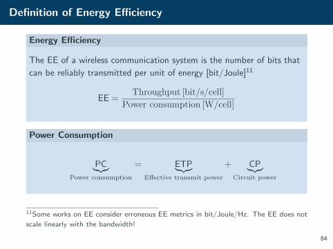
Definition of Energy Efficiency

Energy Efficiency

The EE of a wireless communication system is the number of bits that

can be reliably transmitted per unit of energy [bit/Joule]11

EE =Throughput [bit/s/cell]

Power consumption [W/cell]

Power Consumption

PC︸︷︷︸Power consumption

= ETP︸︷︷︸Effective transmit power

+ CP︸︷︷︸Circuit power

11Some works on EE consider erroneous EE metrics in bit/Joule/Hz. The EE does not

scale linearly with the bandwidth!

84

Circuit Power Model

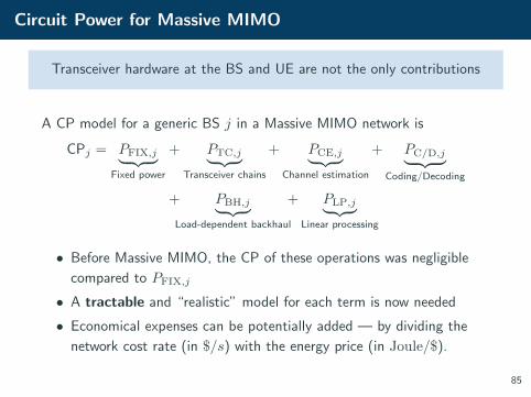
Circuit Power for Massive MIMO

Transceiver hardware at the BS and UE are not the only contributions

A CP model for a generic BS j in a Massive MIMO network is

CPj = PFIX,j︸ ︷︷ ︸Fixed power

+ PTC,j︸ ︷︷ ︸Transceiver chains

+ PCE,j︸ ︷︷ ︸Channel estimation

+ PC/D,j︸ ︷︷ ︸Coding/Decoding

+ PBH,j︸ ︷︷ ︸Load-dependent backhaul

+ PLP,j︸ ︷︷ ︸Linear processing

• Before Massive MIMO, the CP of these operations was negligible

compared to PFIX,j

• A tractable and “realistic” model for each term is now needed

• Economical expenses can be potentially added — by dividing the

network cost rate (in $/s) with the energy price (in Joule/$).

85

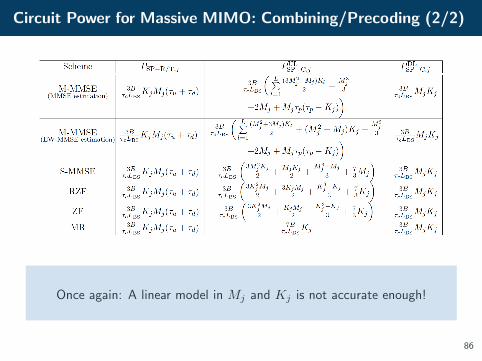
Circuit Power for Massive MIMO: Combining/Precoding (2/2)

Once again: A linear model in Mj and Kj is not accurate enough!

86

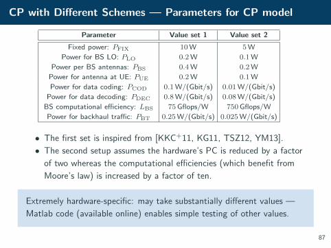
CP with Different Schemes — Parameters for CP model

Parameter Value set 1 Value set 2

Fixed power: PFIX 10W 5W

Power for BS LO: PLO 0.2W 0.1W

Power per BS antennas: PBS 0.4W 0.2W

Power for antenna at UE: PUE 0.2W 0.1W

Power for data coding: PCOD 0.1W/(Gbit/s) 0.01W/(Gbit/s)

Power for data decoding: PDEC 0.8W/(Gbit/s) 0.08W/(Gbit/s)

BS computational efficiency: LBS 75Gflops/W 750Gflops/W

Power for backhaul traffic: PBT 0.25W/(Gbit/s) 0.025W/(Gbit/s)

• The first set is inspired from [KKC+11, KG11, TSZ12, YM13].

• The second setup assumes the hardware’s PC is reduced by a factor

of two whereas the computational efficiencies (which benefit from

Moore’s law) is increased by a factor of ten.

Extremely hardware-specific: may take substantially different values —

Matlab code (available online) enables simple testing of other values.

87

Energy Efficiency and

Throughput Tradeoff

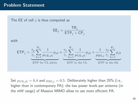
Problem Statement

The EE of cell j is thus computed as

EEj =TRj

ETPj + CPj

with

ETPj =τpτc

Kj∑k=1

1

µUE,jkpjk︸ ︷︷ ︸

ETP for UL pilots

+τuτc

Kj∑k=1

1

µUE,jkpjk︸ ︷︷ ︸

ETP in the UL

+1

µBS,j

τdτc

Kj∑k=1

ρjk︸ ︷︷ ︸ETP in the DL

Set µUE,jk = 0.4 and µBS,j = 0.5. Deliberately higher than 25% (i.e.,

higher than in contemporary PA): the low power levels per antenna (in

the mW range) of Massive MIMO allow to use more efficient PA.

88

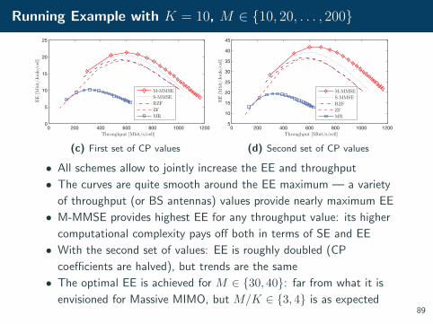
Running Example with K = 10, M ∈ {10, 20, . . . , 200}

0 200 400 600 800 1000 12000

5

10

15

20

25

Throughput [Mbit/s/cell]

EE [M

bit/

Joul

e/ce

ll]

M-MMSES-MMSERZFZFMR

(c) First set of CP values

0 200 400 600 800 1000 12005

10

15

20

25

30

35

40

45

Throughput [Mbit/s/cell]

EE [M

bit/

Joul

e/ce

ll]

M-MMSES-MMSERZFZFMR

(d) Second set of CP values

• All schemes allow to jointly increase the EE and throughput

• The curves are quite smooth around the EE maximum — a variety

of throughput (or BS antennas) values provide nearly maximum EE

• M-MMSE provides highest EE for any throughput value: its higher

computational complexity pays off both in terms of SE and EE

• With the second set of values: EE is roughly doubled (CP

coefficients are halved), but trends are the same

• The optimal EE is achieved for M ∈ {30, 40}: far from what it is

envisioned for Massive MIMO, but M/K ∈ {3, 4} is as expected89

Power Allocation

Utility Function

How to measure network performance?

• There are∑Ll=1Kl UEs, each with UL SE and DL SE

• Combining/precoding and transmit power allocation affect SE

• For given precoding, the DL SEs have a common structure:

SEDLjk =

τdτc

log2

(1 +

ρjkajkL∑l=1

Kl∑i=1

ρliblijk + σ2DL

)for UE k in cell j

ajk = |E{wH

jkhjjk}|2 blijk =

{E{|wH

lihljk|2} (l, i) 6= (j, k)

E{|wH

jkhljk|2} − |E{wH

jkhjjk}|2 (l, i) = (j, k)

Utility function: Maps all SEs into a single performance metric

U(SE11, . . . ,SELKL) =

∑Lj=1

∑Kj

k=1 SEjk Max sum SE

minj,k SEjk Max-min fairness∏Lj=1

∏Kj

k=1 SINRjk Max product SINR

90

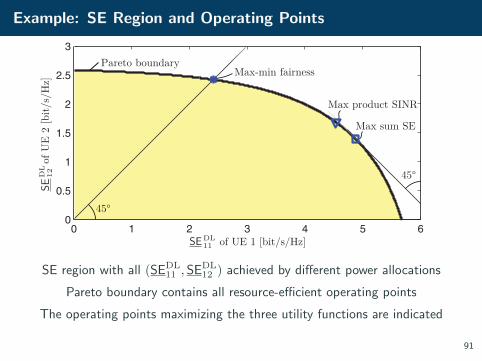
Example: SE Region and Operating Points

0 1 2 3 4 5 60

0.5

1

1.5

2

2.5

3

of UE 1 [bit/s/Hz]

of U

E 2

[bit/

s/H

z]

Max-min fairness

Max sum SE

Max product SINR

45°

45°

Pareto boundary

SE DL11

SED

L12

SE region with all (SEDL11 ,SEDL

12 ) achieved by different power allocations

Pareto boundary contains all resource-efficient operating points

The operating points maximizing the three utility functions are indicated

91

Basic Optimization Theory

Optimization problem on standard form:

maximizex

f0(x)

subject to fn(x) ≤ 0 n = 1, . . . , N

• Optimization variable x = [x1 x2 . . . xV ]T ∈ RV

• Utility function f0 : RV → R• Constraint functions fn : RV → R, n = 1, . . . , N

Solvable to global optimality with standard techniques (CVX, Yalmip) if

• Linear program: f0 and f1, . . . , fN are linear or affine functions

• Geometric program: −f0 and f1− 1, . . . , fN − 1 are posynomials12

• Convex program: −f0 and f1, . . . , fN are convex functions

12fn is posynomial if fn(x) =∑Bb=1 cbx

e1,b1 x

e2,b2 · · ·xeV,b

V for some positive integer

B, constants cb > 0, and exponents e1,b, . . . , eV,b ∈ R for b = 1, . . . , B

92

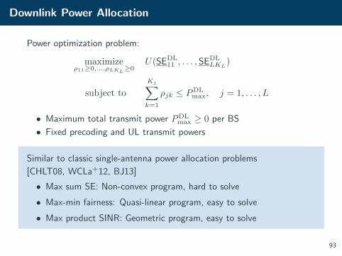
Downlink Power Allocation

Power optimization problem:

maximizeρ11≥0,...,ρLKL

≥0U(SEDL

11 , . . . ,SEDLLKL

)

subject to

Kj∑k=1

ρjk ≤ PDLmax, j = 1, . . . , L

• Maximum total transmit power PDLmax ≥ 0 per BS

• Fixed precoding and UL transmit powers

Similar to classic single-antenna power allocation problems

[CHLT08, WCLa+12, BJ13]

• Max sum SE: Non-convex program, hard to solve

• Max-min fairness: Quasi-linear program, easy to solve

• Max product SINR: Geometric program, easy to solve

93

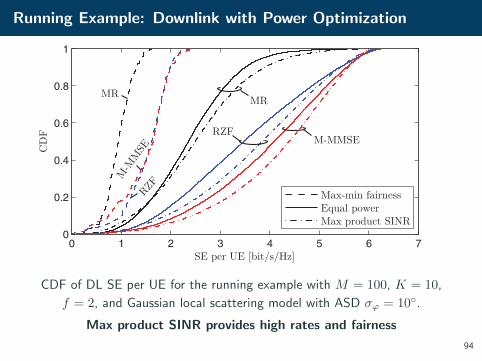
Running Example: Downlink with Power Optimization

0 1 2 3 4 5 6 70

0.2

0.4

0.6

0.8

1

SE per UE [bit/s/Hz]

CD

F

Max-min fairnessEqual powerMax product SINR

M-MMSERZF

MRMR

RZFM

-MM

SE

CDF of DL SE per UE for the running example with M = 100, K = 10,

f = 2, and Gaussian local scattering model with ASD σϕ = 10◦.

Max product SINR provides high rates and fairness

94

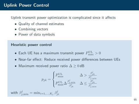
Uplink Power Control

Uplink transmit power optimization is complicated since it affects

• Quality of channel estimates

• Combining vectors

• Power of data symbols

Heuristic power control

• Each UE has a maximum transmit power PULmax > 0

• Near-far effect: Reduce received power differences between UEs

• Maximum received power ratio ∆ ≥ 0 dB

pjk =

PUL

max ∆ >βjjk

βjj,min

PULmax∆

βjj,min

βjjk

∆ ≤ βjjk

βjj,min

with βjj,min = mini=1,...,Kjβjji

95

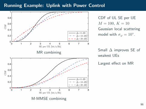
Running Example: Uplink with Power Control

0 1 2 3 4 5 6 7 80

0.2

0.4

0.6

0.8

1

SE per UE [bit/s/Hz]

CD

F

∆=0 dB∆=10 dB∆=20 dB

MR combining

0 1 2 3 4 5 6 7 80

0.2

0.4

0.6

0.8

1

SE per UE [bit/s/Hz]

CD

F

∆=0 dB∆=10 dB∆=20 dB

M-MMSE combining

CDF of UL SE per UE

M = 100, K = 10

Gaussian local scattering

model with σϕ = 10◦.

Small ∆ improves SE of

weakest UEs

Largest effect on MR

96

Case Study

Case Study: Scenario

9 10 11 12

13 14 15 16

1 2

5 6

9 10

13 14

9 10

13 14

3 4

7 8

11 12

15 16

11 12

15 16

1 2

5 6

1 2 3 4

5 6 7 8

3 4

7 8

An arbitrary cell

0.25 km

2 4

5 7

10 12

13 15

1 3

6 8

9 11

14 16

Analyze practical baseline performance with

• 3GPP 3D UMi NLoS channel model13

• Optimized power allocation

• Least-square channel estimation (without channel statistics)

• MR or RZF processing

13Using QuaDRiGa implementation by Fraunhofer Heinrich Hertz Institute97

Array and Transmission Configurations

Maximum transmit power

• Uplink: 20 dBm per UE

• Downlink: 30 dBm per BS

Cylindrical array configurations

(“horizontal × vertical × polarization”):

1. 10× 5× 2 (M = 100)

2. 20× 5× 1 (M = 100)

3. 20× 5× 2 (M = 200)

BS height 25 m, UE height 1.5 m

1) and 2) have same number of RF chains

2) and 3) have same physical size

98

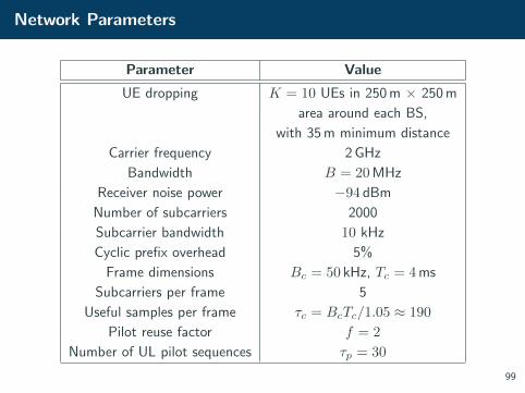
Network Parameters

Parameter Value

UE dropping K = 10 UEs in 250 m × 250 m

area around each BS,

with 35 m minimum distance

Carrier frequency 2 GHz

Bandwidth B = 20 MHz

Receiver noise power −94 dBm

Number of subcarriers 2000

Subcarrier bandwidth 10 kHz

Cyclic prefix overhead 5%

Frame dimensions Bc = 50 kHz, Tc = 4 ms

Subcarriers per frame 5

Useful samples per frame τc = BcTc/1.05 ≈ 190

Pilot reuse factor f = 2

Number of UL pilot sequences τp = 30

99

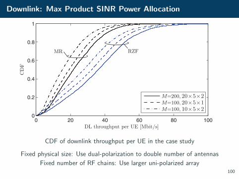
Downlink: Max Product SINR Power Allocation

0 20 40 60 80 1000

0.2

0.4

0.6

0.8

1

DL throughput per UE [Mbit/s]

CD

F

M=200, 20×5×2M=100, 20×5×1M=100, 10×5×2

MR RZF

CDF of downlink throughput per UE in the case study

Fixed physical size: Use dual-polarization to double number of antennas

Fixed number of RF chains: Use larger uni-polarized array100

Uplink: Heuristic power control ∆ = 20 dB

0 10 20 30 40 500

0.2

0.4

0.6

0.8

1

UL throughput per UE [Mbit/s]

CD

F

M=200, 20×5×2M=100, 20×5×1M=100, 10×5×2

MR

RZF

CDF of uplink throughput per UE in the case study

Similar observations as in downlink

101

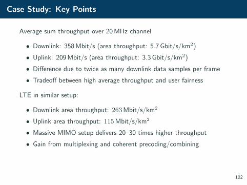
Case Study: Key Points

Average sum throughput over 20 MHz channel

• Downlink: 358 Mbit/s (area throughput: 5.7 Gbit/s/km2)

• Uplink: 209 Mbit/s (area throughput: 3.3 Gbit/s/km2)

• Difference due to twice as many downlink data samples per frame

• Tradeoff between high average throughput and user fairness

LTE in similar setup:

• Downlink area throughput: 263 Mbit/s/km2

• Uplink area throughput: 115 Mbit/s/km2

• Massive MIMO setup delivers 20–30 times higher throughput

• Gain from multiplexing and coherent precoding/combining

102

Open Problems

Goldmine of Open Problems

Massive MIMO is a mature research field, no low-hanging fruits!

Make Massive MIMO work in FDD mode

• Long-standing challenge. Is it practically feasible to exploit sparsity?

Channel measurements, channel modeling, data traffic modeling

• Required for system level simulations

Cross-layer system design

• Protocols for random access and system information broadcast

• Spatial resource allocation

• Power control balancing sum SE and fairness

• Estimation of spatial correlation properties under mobility

103

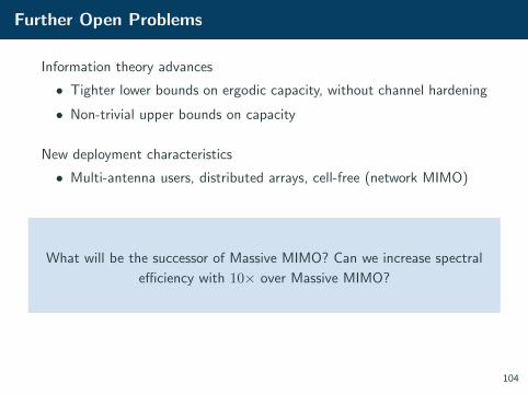
Further Open Problems

Information theory advances

• Tighter lower bounds on ergodic capacity, without channel hardening

• Non-trivial upper bounds on capacity

New deployment characteristics

• Multi-antenna users, distributed arrays, cell-free (network MIMO)

What will be the successor of Massive MIMO? Can we increase spectral

efficiency with 10× over Massive MIMO?

104

References i

[AMVW91] S. Anderson, M. Millnert, M. Viberg, and B. Wahlberg, “An

adaptive array for mobile communication systems,” IEEE

Trans. Veh. Technol., vol. 40, no. 1, pp. 230–236, 1991.

[BHS18] E. Bjornson, J. Hoydis, and L. Sanguinetti, “Massive MIMO

has unlimited capacity,” IEEE Trans. Wireless Commun.,

2018.

[BJ13] E. Bjornson and E. Jorswieck, “Optimal resource allocation in

coordinated multi-cell systems,” Foundations and Trends in

Communications and Information Theory, vol. 9, no. 2-3, pp.

113–381, 2013.

[CHLT08] M. Chiang, P. Hande, T. Lan, and C. Tan, “Power control in

wireless cellular networks,” Foundations and Trends in

Networking, vol. 2, no. 4, pp. 355–580, 2008.

105

References ii

[GERT11] X. Gao, O. Edfors, F. Rusek, and F. Tufvesson, “Linear

pre-coding performance in measured very-large MIMO

channels,” in Proc. IEEE VTC Fall, 2011.

[GJ11] B. Gopalakrishnan and N. Jindal, “An analysis of pilot

contamination on multi-user MIMO cellular systems with

many antennas,” in Proc. IEEE SPAWC, 2011.

[HCPR12] H. Huh, G. Caire, H. Papadopoulos, and S. Ramprashad,

“Achieving “massive MIMO” spectral efficiency with a

not-so-large number of antennas,” IEEE Trans. Wireless

Commun., vol. 11, no. 9, pp. 3226–3239, 2012.

[HHWtB12] J. Hoydis, C. Hoek, T. Wild, and S. ten Brink, “Channel

measurements for large antenna arrays,” in Proc. IEEE

ISWCS, 2012.

106

References iii

[JAMV11] J. Jose, A. Ashikhmin, T. L. Marzetta, and S. Vishwanath,

“Pilot contamination and precoding in multi-cell TDD

systems,” IEEE Trans. Commun., vol. 10, no. 8, pp.

2640–2651, 2011.

[KG11] R. Kumar and J. Gurugubelli, “How green the LTE technology

can be?” in Proc. Wireless VITAE, 2011.

[KKC+11] D. Kang, D. Kim, Y. Cho, J. Kim, B. Park, C. Zhao, and

B. Kim, “1.6 - 2.1 GHz broadband Doherty power amplifiers

for LTE handset applications,” in Proc. IEEE MTT-S, June

2011, pp. 1–4.

[Mar10] T. L. Marzetta, “Noncooperative cellular wireless with

unlimited numbers of base station antennas,” IEEE Trans.

Wireless Commun., vol. 9, no. 11, pp. 3590–3600, 2010.

107

References iv

[Qua12] Qualcomm, “Rising to meet the 1000x mobile data

challenge,” Qualcomm Incorporated, Tech. Rep., 2012.

[SBEM90] S. C. Swales, M. A. Beach, D. J. Edwards, and J. P.

McGeehan, “The performance enhancement of multibeam

adaptive base-station antennas for cellular land mobile radio

systems,” IEEE Trans. Veh. Technol., vol. 39, no. 1, pp.

56–67, 1990.

[TSZ12] S. Tombaz, K. W. Sung, and J. Zander, “Impact of

densification on energy efficiency in wireless access networks,”

in Proc. IEEE GLOBECOM Workshop, Dec 2012, pp. 57–62.

108

References v

[WCLa+12] P. Weeraddana, M. Codreanu, M. Latva-aho,

A. Ephremides, and C. Fischione, “Weighted sum-rate

maximization in wireless networks: A review,” Foundations

and Trends in Networking, vol. 6, no. 1-2, pp. 1–163, 2012.

[Win87] J. H. Winters, “Optimum combining for indoor radio systems

with multiple users,” IEEE Trans. Commun., vol. 35, no. 11,

pp. 1222–1230, 1987.

[YGFL13] H. Yin, D. Gesbert, M. Filippou, and Y. Liu, “A coordinated

approach to channel estimation in large-scale multiple-antenna

systems,” IEEE J. Sel. Areas Commun., vol. 31, no. 2, pp.

264–273, 2013.

109

References vi

[YM13] H. Yang and T. L. Marzetta, “Total energy efficiency of

cellular large scale antenna system multiple access mobile

networks,” in Proc. IEEE Online GreenComm, 2013, pp.

27–32.

110