Embed Size (px)
Citation preview
Faculty of Science and Technology
MASTER’S THESIS
Study program:
MSc in Offshore Technology
Specialization:
Marine and Subsea Technology
Spring semester, 2015
Open access
Writer: Velarasan Masilamani
………………………………………… (Writer’s signature)
Faculty supervisor: Ove Tobias Gudmestad
External supervisor(s):
Thesis title:
Vortex Induced Vibration (VIV) Analysis of Subsea Jumper Spools
Credits (ECTS): 30
Key words:
Vortex Induced Vibration (VIV)
Subsea
Jumper Spools
Finite Element Analysis
ANSYS
DNV-RP-F105
DNV-RP-C203
Fatigue Life Assessment
Pages: 75
+ enclosure: 125
Stavanger, June 15, 2015
VIV ANALYSIS OF SUBSEA JUMPER SPOOLS
i
ABSTRACT
Subsea rigid jumpers are usually rigid steel pipe sections that provide the interface between
subsea structures, such as pipelines to manifolds, trees to flowlines and pipelines to risers. Each
jumper shall be designed such that it is flexible enough to allow the expansion and contraction of
the flowline or the pipeline due to the change in pressure rating and/or end thermal expansion
and to accommodate the installation misalignment. In addition, the subsea jumper design should
also be rigid enough to meet the external environmental loads.
The ability of the jumper system to accommodate these loads is achieved through its design
procedure, which includes strength and fatigue analysis. The former defines the required
configuration of the jumper system based on the end displacement tolerance requirements, with
the least flexibility possible and the latter helps to determine the fatigue life of the system to
satisfy the design life. Based on the field specific conditions and end displacement requirements,
any geometry of the jumper can be used in the field architecture. The usual types of jumper
configurations used in the industry are free span, M-shape, Z-shape and inverted U-shaped.
Although some designers consider these jumper systems as static elements, they are in fact
susceptible to fatigue loading. This arises from the complex jumper configurations with longer
unsupported lengths of the pipe section. Though the complexity is advantageous with regard to
the displacement tolerance, they bring their own unique challenges from a fatigue loading
perspective.
The objective of this project is to perform a sensitivity study, of the fatigue damage due to vortex
induced vibration (VIV), on the typical subsea jumper system. Even though there are other
modes, which can cause fatigue damage to the jumpers, like the thermal cyclic loading from
flowlines, slugging effect and fluid induced vibrations, this report is confined only to the fatigue
damage due to VIV. A comprehensive study of a specific case has been carried out to
demonstrate the effects of VIV on a subsea jumper spool. The results are extended to general
spool geometries whenever possible. The sensitivity study will assess the key parameters, like
the jumper configuration, seabed current velocity and the angle of the current flow to understand
the case specific severity of the fatigue damage. This analysis is performed based on the
background principle followed in DNV-RP-F105 and using the finite element analysis (FEA)
tool ANSYS.
Based on the observations from the sensitivity study, we understand that from the fatigue life of
the typical jumper system, we can define the case specific critical length of the jumper. This
critical length identification helps to understand the cases that require the use of the VIV
mitigation measures. It is also observed that for the same jumper configuration under the same
seabed current condition, the fatigue life would be different based on the angle of current flow
and the yearly probability of occurrence of the seabed current velocity.

VIV ANALYSIS OF SUBSEA JUMPER SPOOLS
ii
ACKNOWLEDGEMENT
I take this opportunity to express my sincere gratitude to the following persons for their valuable
contribution and support, in helping me to turn this thesis thought into a valuable piece of work.
First and foremost, my heartfelt gratitude to my supervisor Professor Ove T. Gudmestad, who
in-spite of being extraordinarily busy with his duties, took time out to hear and guide my thesis
throughout the period. The tasks that are accomplished in this work would have never been
possible without his advice and suggestions. Without his comments and remarks, the
presentation of this report could have never been perfected. Of all the above, he has always been
a person of inspiration to me, to challenge the challenges in life.
Secondly, I would like to express my deepest thanks to Dr. Daniel Karunakaran for his
suggestions on the documents to refer, to understand the physics behind the work and also for his
advice on framing the work. My special thanks to Mr. Goutam Marath of J P Kenny, who
introduced me to this topic and also supported me all the way to accomplish the tasks.
Furthermore, I express my radiant sentiment of thanks to my parents, for their love, affection,
moral support and guidance throughout my life. Last but not least, I thank all my friends of
Stavanger, who made my stay in Norway a fun-filled and magnificent one, with lots of memories
to carry for the rest of my life.
Finally, I would like to devote all my credits of this thesis work to GOD, who provided me good
health and living, throughout the way in completing this thesis.
VIV ANALYSIS OF SUBSEA JUMPER SPOOLS
iii
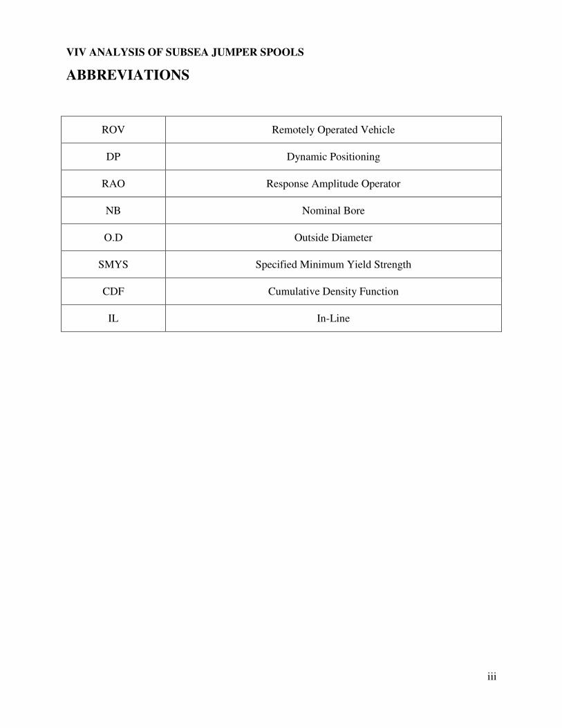
ABBREVIATIONS
ROV Remotely Operated Vehicle
DP Dynamic Positioning
RAO Response Amplitude Operator
NB Nominal Bore
O.D Outside Diameter
SMYS Specified Minimum Yield Strength
CDF Cumulative Density Function
IL In-Line
VIV ANALYSIS OF SUBSEA JUMPER SPOOLS
iv
Table of Contents
ABSTRACT ..................................................................................................................................... i
ACKNOWLEDGEMENT .............................................................................................................. ii
ABBREVIATIONS ....................................................................................................................... iii
List of Tables ............................................................................................................................... viii
List of Figures ................................................................................................................................ ix
CHAPTER-1 ................................................................................................................................... 1
INTRODUCTION .......................................................................................................................... 1
1.1 Background ........................................................................................................................... 1
1.2 Motivation ............................................................................................................................. 1
1.3 Scope ..................................................................................................................................... 2
1.4 Limitation .............................................................................................................................. 2
1.5 Organization of the Report .................................................................................................... 3
CHAPTER-2 ................................................................................................................................... 4
OVERVIEW OF THE PIPELINES AND TIE-IN SPOOLS ......................................................... 4
2.1 Pipelines ................................................................................................................................ 4
2.2 Classification of Offshore Pipelines ...................................................................................... 4
2.3 Pipeline Design ..................................................................................................................... 5
2.4 Pipeline Installation ............................................................................................................... 6
2.4.1 S-lay ................................................................................................................................ 6
2.4.2 J-lay ................................................................................................................................ 6
2.4.3 Reel barge ....................................................................................................................... 6
2.4.4 Tow-in ............................................................................................................................ 7
2.4.4.1 Surface tow .............................................................................................................. 7
2.4.4.2 Mid-depth tow .......................................................................................................... 7
2.4.4.3 Off-bottom tow ........................................................................................................ 7
2.4.4.4 Bottom tow............................................................................................................... 7
2.5 Pipeline Stresses .................................................................................................................. 11
2.6 Tie-in Spools ....................................................................................................................... 12
2.7 Types of Tie-in Spools ........................................................................................................ 13
VIV ANALYSIS OF SUBSEA JUMPER SPOOLS
v
2.7.1 Vertical Tie-in Systems ................................................................................................ 13
2.7.2 Horizontal Tie-in Systems ............................................................................................ 13
CHAPTER 3 ................................................................................................................................. 16
VIV PHENOMENON .................................................................................................................. 16
3.1 Vortex Formation ................................................................................................................ 16
3.1.1 Factors Influencing Vortex Induced Vibrations ........................................................... 16
3.1.2 Physics behind Vortex Formation ................................................................................ 16
3.1.3 Factors Influencing Vortices Intensity ......................................................................... 17
3.2 Parameters to define the vortex significance....................................................................... 18
3.2.1 Fluid Parameters ........................................................................................................... 18
3.2.1.1 Reynolds Number (Re) .......................................................................................... 18
3.2.1.2 Keulegen-Carpenter Number (KC) ........................................................................ 18
3.2.1.3 Current Flow Velocity ratio ................................................................................... 20
3.2.1.4 Turbulence Intensity .............................................................................................. 20
3.2.1.5 Shear Fraction of Flow Profile ............................................................................... 20
3.2.2 Fluid Structure Interface (FSI) Parameters ................................................................... 20
3.2.2.1 Reduced Velocity ................................................................................................... 21
3.2.2.2 Stability Parameter ................................................................................................. 22
3.2.2.3 Strouhal Number (S) .............................................................................................. 24
3.2.3 Structure Parameters ..................................................................................................... 25
3.2.3.1 Geometry................................................................................................................ 25
3.2.3.2 Mass Ratio ............................................................................................................. 25
3.2.3.3 Damping Factor ..................................................................................................... 26
3.3 “Lock-in” Phenomenon ....................................................................................................... 26
3.4 Types of Vortex Induced Vibrations ................................................................................... 27
3.4.1 In-line VIV ................................................................................................................... 27
3.4.2 Cross-Flow VIV ........................................................................................................... 28
3.5 Impact of the cylinder oscillatory motion on wakes ........................................................... 30
3.6 VIV Mitigation .................................................................................................................... 35
3.6.1 Increased Stability Parameter ....................................................................................... 35
3.6.2 Avoiding Resonance ..................................................................................................... 35
VIV ANALYSIS OF SUBSEA JUMPER SPOOLS
vi
3.6.3 Streamline Cross Section .............................................................................................. 35
3.6.4 Add a Vortex Suppression Device................................................................................ 36
CHAPTER 4 ................................................................................................................................. 37
ANALYSIS METHODOLOGY ................................................................................................... 37
4.1 Modal Analysis on ANSYS ................................................................................................ 37
4.2 VIV Analysis ....................................................................................................................... 38
4.2.1 Environmental Modeling .............................................................................................. 38
4.2.1.1 Current ................................................................................................................... 38
4.2.1.2 Waves ..................................................................................................................... 39
4.2.2 Response Modeling ...................................................................................................... 43
4.2.2.1 Inline Response Modeling ..................................................................................... 43
4.2.2.2 Cross-flow Response Modeling ............................................................................. 46
4.3 VIV Analysis Criterion ....................................................................................................... 49
4.3.1 Inline VIV fatigue criterion .......................................................................................... 49
4.3.2 Cross-flow VIV fatigue criterion .................................................................................. 50
4.3.3 Direct Wave Induced VIV fatigue criterion ................................................................. 50
4.4 Workflow for VIV Assessment ........................................................................................... 50
4.5 Assessment of Fatigue life .................................................................................................. 52
CHAPTER 5 ................................................................................................................................. 55
ASSUMPTIONS ........................................................................................................................... 55
CHAPTER 6 ................................................................................................................................. 57
SENSITIVITY ANALYSIS ......................................................................................................... 57
CHAPTER 7 ................................................................................................................................. 67
DISCUSSION ............................................................................................................................... 67
7.1 Under In-Plane Current Condition ...................................................................................... 67
7.2 Under Out-of-Plane Current Condition ............................................................................... 68
7.3 Uncertainty .......................................................................................................................... 69
CHAPTER 8 ................................................................................................................................. 70
CONCLUSION AND RECOMMENDATION ............................................................................ 70
CHAPTER 9 ................................................................................................................................. 72

VIV ANALYSIS OF SUBSEA JUMPER SPOOLS
vii
REFERENCE ................................................................................................................................ 72
ANNEXURES .............................................................................................................................. 75
VIV ANALYSIS OF SUBSEA JUMPER SPOOLS
viii
List of Tables
Table 1 - Condition for Water Depth Categorization .................................................................. 42
Table 2 - Horizontal Water Particle Velocity based on Water Depth category ........................... 42
Table 3 - Safety factors for Natural Frequencies ......................................................................... 45
Table 4 - General Safety factors for Fatigue ................................................................................ 46
Table 5 - Safety factors for Screening Criterion .......................................................................... 50
Table 6 - Parameters to define the Jumper S-N curve ................................................................. 53
Table 7 - Matrix of the Sensitivity Analysis performed ............................................................... 57
Table 8 - Variation in the jumper oscillation type based on current flow pattern ........................ 58
VIV ANALYSIS OF SUBSEA JUMPER SPOOLS
ix
List of Figures
Figure 1 - Types of Pipelines ......................................................................................................... 5
Figure 2- S-Lay Method of Pipeline Installation ........................................................................... 8
Figure 3 - J-Lay Method of Pipeline Installation ........................................................................... 8
Figure 4 - Surface Tow Method of Pipeline Installation ............................................................... 9
Figure 5 - Mid-Depth Tow Method of Pipeline Installation .......................................................... 9
Figure 6 - Off-Bottom Tow Method of Pipeline Installation ....................................................... 10
Figure 7 - Bottom Tow Method of Pipeline Installation .............................................................. 10
Figure 8 – Horizontal tie-in system ............................................................................................. 14
Figure 9 – Sequence of installation for horizontal tie-in system ................................................. 15
Figure 10 - Variation in vortex pattern based on Reynolds number (Re) . ................................... 19
Figure 11 - Variation of the Eigen frequency w.r.t span length under different boundary
conditions for a cylinder of O.D = 500 mm . ................................................................................ 22
Figure 12 - Cross-Flow Reduced Velocity variation w.r.t Reynolds number ............................. 23
Figure 13 - In-line Reduced Velocity variation w.r.t Stability Parameter ................................... 24
Figure 14 - Variation in Strouhal Number (S) w.r.t Reynolds Number (Re) . ............................. 25
Figure 15 - Wake formation pattern for 1/3rd
of the vortex shedding cycle . ............................... 28
Figure 16 – VIV exposure area of the Jumper for the Out-of-Plane current condition ................ 29
Figure 17 - VIV exposure area of the Jumper for the In-Plane current condition ........................ 30
Figure 18 - Variation of the “Lock-in” range based on Cylinder Amplitude (Ay ...................... 31
Figure 19 - Stable vortex shedding pattern for Re = 190 and when � = . .......................... 32
Figure 20 - Unstable vortex shedding pattern for Re = 190 and when � = . ...................... 32
Figure 21 - Drag Coefficient increase based on Vibration Amplitude at a frequency equal to the
shedding frequency ...................................................................................................................... 33
Figure 22 - Drag coefficient variation based on Reynolds number in a steady flow for smooth
circular cylinder ........................................................................................................................... 33
Figure 23 - Types of Jumper Oscillations .................................................................................... 37
Figure 24 - Inline Response Model Generation Principle ........................................................... 44
Figure 25 - Cross-flow Response Model Generation Principle ................................................... 47
Figure 26 - Relation between d, e and D ..................................................................................... 48
VIV ANALYSIS OF SUBSEA JUMPER SPOOLS
x
Figure 27 - Flowchart over design checks for a free span ........................................................... 51
Figure 28 - Overview of main components in a free span assessment ........................................ 51
Figure 29 - Eigen frequency variations based on the mode number and the jumper length ......... 57
Figure 30 - Case specific sea bottom current velocities on a long-term distribution basis .......... 58
Figure 31 - Variation of Reduced Velocity (Vr) for the 30m Jumper profile ............................... 59
Figure 32 - Variation of Reduced Velocity (Vr) for the 34m Jumper profile ............................... 59
Figure 33 - Variation of Reduced Velocity (Vr) for the 38m Jumper profile ............................... 60
Figure 34 - Configurations specific In-line Oscillation amplitude ............................................... 61
Figure 35 - Variation of the Unit Amplitude Stresses based on the jumper configurations ......... 61
Figure 36 - Configurations specific In-line Oscillation Stress Range .......................................... 62
Figure 37 - Fatigue life variations for the Out-of-Plane current flow........................................... 63
Figure 38 - Fatigue life variations for the In-Plane current flow .................................................. 64
Figure 39 - Configurations specific fatigue life variation - 1 ....................................................... 65
Figure 40 - Configurations specific fatigue life variation - 2 ....................................................... 65
Figure 41 - Configurations specific fatigue life variation – 3 ....................................................... 66
VIV ANALYSIS OF SUBSEA JUMPER SPOOLS
1
CHAPTER-1
INTRODUCTION
1.1 Background
In the oil and gas industry, pipelines are used to transport the hydrocarbons from the source to
the destination. Based on the type of the function involved, these pipelines can vary from a small
bore inter-field flowline to a large bore trunk export pipeline. Normally, when these pipelines are
installed in the field, the final connection between the pipeline end termination (PLET) and the
destination is performed through the use of a Tie-in spool. This is due to the pipeline installation
limitations from the various field specific factors.
Therefore, these tie-in spools should also satisfy the design life requirement of the pipelines, in
order to ensure that it performs its intended purpose, without any hydrocarbon leakage, though
out the service life. Even though, the mechanical design of the jumper, which depends on the
following factors like,
Pipeline end thermal movement
Pipeline installation misalignment and
Connecting hubs reaction force limitations
satisfies the design life of the system, through proper selection of the jumper configuration and
integrity checks. It is also necessary to make sure that the fatigue life of the jumper satisfies the
design life requirement. This is because, the occurrence of seabed current, makes the large
unsupported configuration of the jumpers, more prone to vibrations, which can result in fatigue
damage of the system.
Based on the jumper configuration and the seabed current profile involved, the severity of the
jumper fatigue life would differ. Therefore, it is always a must to make sure that the jumper
system satisfies the fatigue life requirements in addition to the mechanical design integrity
checks for design life.
1.2 Motivation
Even though VIV assessment of long, slender structures may be considered sufficiently mature,
it is noted lately that the industry is increasingly considering complex jumper systems, wherein
the structure may comprise of pipe sections of various orientations. However, there are currently
neither a guideline for the design like the DNV-RP-F105, which presents the free spanning
analysis for the subsea pipelines, nor a prominent software such as FatFree (DNV software) or
Shear7, which are specially designed for the riser systems, that may directly be used to estimate
VIV ANALYSIS OF SUBSEA JUMPER SPOOLS
2
the VIV fatigue damage for the non-straight pipe configurations like in the case of subsea
jumpers.
1.3 Scope
As mentioned in the section-1 of DNV-RP-F105,
“Basic principles may also be applied to more complex cross sections such as pipe-in-pipe,
bundles, flexible pipes and umbilicals”
“The fundamental principles given in this RP may also be applied and extended to other offshore
elements such as cylindrical structural elements of the jacket…..”
This thesis is performed based on the basic free spanning principle, as mentioned in DNV-RP-
F105 and it also using the finite element analysis (FEA) tool ANSYS.
The purpose of this thesis is to,
Perform a sensitivity study on the fatigue life of the typical jumper system due to the VIV
phenomenon.
Observe the fatigue life variation based on the assessment of the key parameters like
jumper configuration, seabed current and the angle of the current flow.
Compare the fatigue life of the same system under the same seabed current condition, but
based on the difference in the yearly probability of current velocity occurrence.
Discuss about the variation in the critical length of the jumper based on the case specific
conditions with respect to the angle of the current flow.
Conclude the results from the sensitivity study and make future recommendations of
possible work extension.
1.4 Limitation
Since, this thesis is performed for a typical M-shaped jumper configuration the results of this
work involve the following limitations,
Percentage of occurrence of the in-line oscillation under a cross-flow excitation mode
(or) the cross-flow oscillation under an in-line excitation mode.
Any change in the angle of current flow, from either pure in-plane (or) out-of-plane
current flow.
Any change in the field specific environmental condition, content of transport and
configuration of the jumper, from the assumed conditions in this work.
Any change in the safety zone classification, based on the location of operation.
VIV ANALYSIS OF SUBSEA JUMPER SPOOLS
3
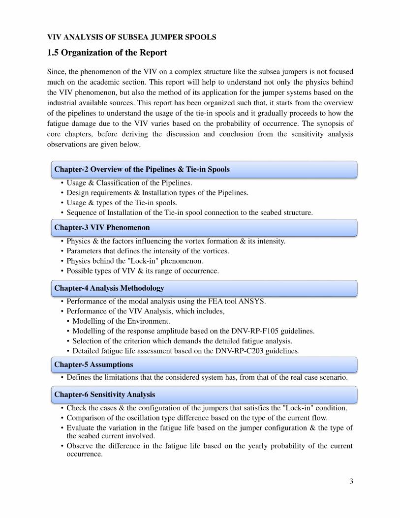
1.5 Organization of the Report
Since, the phenomenon of the VIV on a complex structure like the subsea jumpers is not focused
much on the academic section. This report will help to understand not only the physics behind
the VIV phenomenon, but also the method of its application for the jumper systems based on the
industrial available sources. This report has been organized such that, it starts from the overview
of the pipelines to understand the usage of the tie-in spools and it gradually proceeds to how the
fatigue damage due to the VIV varies based on the probability of occurrence. The synopsis of
core chapters, before deriving the discussion and conclusion from the sensitivity analysis
observations are given below.
Chapter-2 Overview of the Pipelines & Tie-in Spools
• Usage & Classification of the Pipelines.
• Design requirements & Installation types of the Pipelines.
• Usage & types of the Tie-in spools.
• Sequence of Installation of the Tie-in spool connection to the seabed structure.
Chapter-3 VIV Phenomenon
• Physics & the factors influencing the vortex formation & its intensity.
• Parameters that defines the intensity of the vortices.
• Physics behind the "Lock-in" phenomenon.
• Possible types of VIV & its range of occurrence.
Chapter-4 Analysis Methodology
• Performance of the modal analysis using the FEA tool ANSYS.
• Performance of the VIV Analysis, which includes,
• Modelling of the Environment.
• Modelling of the response amplitude based on the DNV-RP-F105 guidelines.
• Selection of the criterion which demands the detailed fatigue analysis.
• Detailed fatigue life assessment based on the DNV-RP-C203 guidelines.
Chapter-5 Assumptions
• Defines the limitations that the considered system has, from that of the real case scenario.
Chapter-6 Sensitivity Analysis
• Check the cases & the configuration of the jumpers that satisfies the "Lock-in" condition.
• Comparison of the oscillation type difference based on the type of the current flow.
• Evaluate the variation in the fatigue life based on the jumper configuration & the type of the seabed current involved.
• Observe the difference in the fatigue life based on the yearly probability of the current occurrence.
VIV ANALYSIS OF SUBSEA JUMPER SPOOLS
4
CHAPTER-2
OVERVIEW OF THE PIPELINES AND TIE-IN SPOOLS
2.1 Pipelines
In the oil and gas industry, Pipelines are one of the ways to transport a fluid that is chemically
stable like the crude (or) refined petroleum, from one place to the other, that are physically
separated by a long distance. In general, the industry uses three essential ways of transportation,
which includes,
Tanker/Shuttle – Here, the fluid is filled and sealed in the tanks and transported to the
required destination.
Pipelines – Here, the fluid is pumped along the pipeline that is constructed between the
source and the destination.
Combination – This works in combination with either of the above two methods, here the
fluid is transformed into either a solid or to another fluid form and then it is transported
through either of the above two methods.
The preference to choose the pipelines, over any other types of transportation is due to the
advantages listed below,
The oil spill rate in the case of the pipelines is less than any other type of transportation.
The cost involved in the oil and gas transported through the pipeline is less in comparison
to the others.
Pipelines are much safe and environment friendly.
Least energy requirement.
Low maintenance cost.
High reliability and
Minimal impact on the land use pattern.
2.2 Classification of Offshore Pipelines
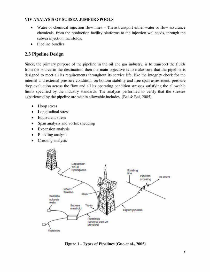
Based on the nature of the fluid that is transported, pipelines can be termed as, (see figure: 1)
(Bai & Bai, 2012 & Guo, Song, Chacko & Ghalambor, 2005),
Export pipelines – These transport either refined (or) crude products (oil and gas) from
the production facility platforms to the shore terminal facilities.
Flow-lines – These transport oil and/or gas from the satellite subsea wells to the subsea
manifolds, from subsea manifolds to production facility platforms and also between
production facility platforms.
VIV ANALYSIS OF SUBSEA JUMPER SPOOLS
5
Water or chemical injection flow-lines – These transport either water or flow assurance
chemicals, from the production facility platforms to the injection wellheads, through the
subsea injection manifolds.
Pipeline bundles.
2.3 Pipeline Design
Since, the primary purpose of the pipeline in the oil and gas industry, is to transport the fluids
from the source to the destination, then the main objective is to make sure that the pipeline is
designed to meet all its requirements throughout its service life, like the integrity check for the
internal and external pressure condition, on-bottom stability and free span assessment, pressure
drop evaluation across the flow and all its operating condition stresses satisfying the allowable
limits specified by the industry standards. The analysis performed to verify that the stresses
experienced by the pipeline are within allowable includes, (Bai & Bai, 2005)
Hoop stress
Longitudinal stress
Equivalent stress
Span analysis and vortex shedding
Expansion analysis
Buckling analysis
Crossing analysis
Figure 1 - Types of Pipelines (Guo et al., 2005)
VIV ANALYSIS OF SUBSEA JUMPER SPOOLS
6
2.4 Pipeline Installation
Once the pipeline is designed, constructed and fabricated. It is then transported and installed at
the site by one of the several installation methods available, which includes, (Guo et al., 2005)
S-lay
J-lay
Reel barge and
Tow-in
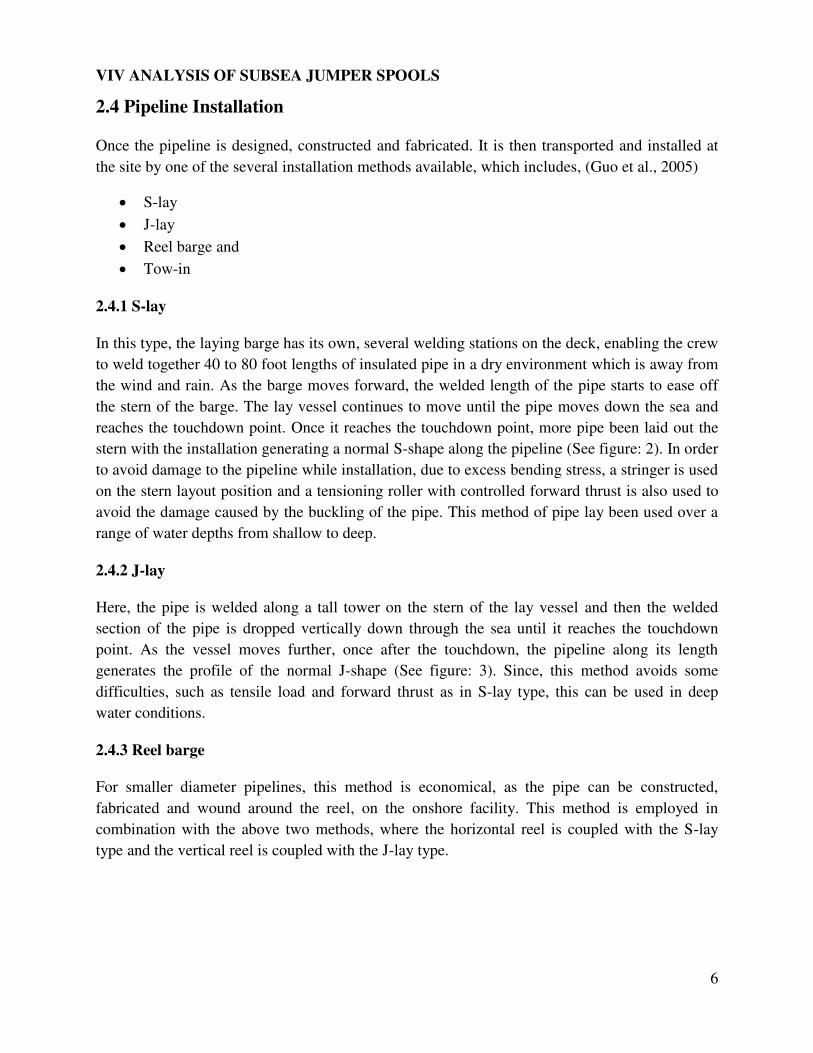
2.4.1 S-lay
In this type, the laying barge has its own, several welding stations on the deck, enabling the crew
to weld together 40 to 80 foot lengths of insulated pipe in a dry environment which is away from
the wind and rain. As the barge moves forward, the welded length of the pipe starts to ease off
the stern of the barge. The lay vessel continues to move until the pipe moves down the sea and
reaches the touchdown point. Once it reaches the touchdown point, more pipe been laid out the
stern with the installation generating a normal S-shape along the pipeline (See figure: 2). In order
to avoid damage to the pipeline while installation, due to excess bending stress, a stringer is used
on the stern layout position and a tensioning roller with controlled forward thrust is also used to
avoid the damage caused by the buckling of the pipe. This method of pipe lay been used over a
range of water depths from shallow to deep.
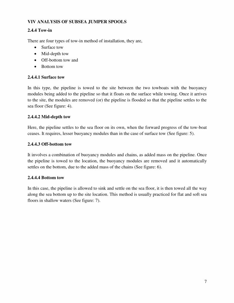
2.4.2 J-lay
Here, the pipe is welded along a tall tower on the stern of the lay vessel and then the welded
section of the pipe is dropped vertically down through the sea until it reaches the touchdown
point. As the vessel moves further, once after the touchdown, the pipeline along its length
generates the profile of the normal J-shape (See figure: 3). Since, this method avoids some
difficulties, such as tensile load and forward thrust as in S-lay type, this can be used in deep
water conditions.
2.4.3 Reel barge
For smaller diameter pipelines, this method is economical, as the pipe can be constructed,
fabricated and wound around the reel, on the onshore facility. This method is employed in
combination with the above two methods, where the horizontal reel is coupled with the S-lay
type and the vertical reel is coupled with the J-lay type.
VIV ANALYSIS OF SUBSEA JUMPER SPOOLS
7
2.4.4 Tow-in
There are four types of tow-in method of installation, they are,
Surface tow
Mid-depth tow
Off-bottom tow and
Bottom tow
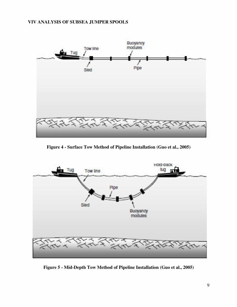
2.4.4.1 Surface tow
In this type, the pipeline is towed to the site between the two towboats with the buoyancy
modules being added to the pipeline so that it floats on the surface while towing. Once it arrives
to the site, the modules are removed (or) the pipeline is flooded so that the pipeline settles to the
sea floor (See figure: 4).
2.4.4.2 Mid-depth tow
Here, the pipeline settles to the sea floor on its own, when the forward progress of the tow-boat
ceases. It requires, lesser buoyancy modules than in the case of surface tow (See figure: 5).
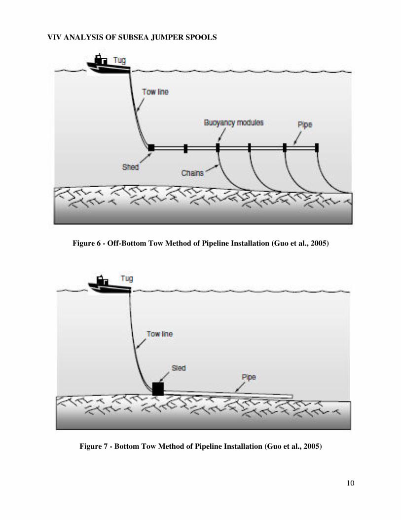
2.4.4.3 Off-bottom tow
It involves a combination of buoyancy modules and chains, as added mass on the pipeline. Once
the pipeline is towed to the location, the buoyancy modules are removed and it automatically
settles on the bottom, due to the added mass of the chains (See figure: 6).
2.4.4.4 Bottom tow
In this case, the pipeline is allowed to sink and settle on the sea floor, it is then towed all the way
along the sea bottom up to the site location. This method is usually practiced for flat and soft sea
floors in shallow waters (See figure: 7).
VIV ANALYSIS OF SUBSEA JUMPER SPOOLS
8
Figure 2- S-Lay Method of Pipeline Installation (Guo et al., 2005)
Figure 3 - J-Lay Method of Pipeline Installation (Guo et al., 2005)
VIV ANALYSIS OF SUBSEA JUMPER SPOOLS
9
Figure 4 - Surface Tow Method of Pipeline Installation (Guo et al., 2005)
Figure 5 - Mid-Depth Tow Method of Pipeline Installation (Guo et al., 2005)
VIV ANALYSIS OF SUBSEA JUMPER SPOOLS
10
Figure 6 - Off-Bottom Tow Method of Pipeline Installation (Guo et al., 2005)
Figure 7 - Bottom Tow Method of Pipeline Installation (Guo et al., 2005)
VIV ANALYSIS OF SUBSEA JUMPER SPOOLS
11
2.5 Pipeline Stresses
Once the installed pipeline comes into operation, the pipeline, which is a form of a pressure
vessel, will experience some stresses due to differential pressure and temperature, between the
pipeline operating condition and the surrounding medium. These stresses act both
circumferential and longitudinal to the pipeline. The component of the stress acting along the
circumference is due to the pressure differential in the pipeline. This stress buildup is usually
restrained by the integrity of the pipeline. This also helps to understand that to which category
does the pipeline belongs to, whether is it thin walled (or) thick walled pipeline. Another
component of the stress acting along the longitudinal axis of the pipeline arises from the
temperature gradient between the maximum operating temperature in the pipeline and the
minimum installed temperature. The longitudinal strain of the pipeline in general is given by
equation 2.5 (a), (Palmer & King, 2004 & Guo et al., 2005) = ∗ ∆T……………�qn . a
Here, = . ℎ ℎ . ∆ = = − =
If incase, the generated longitudinal strain due to temperature difference is restrained ( = by
the boundary conditions of the pipeline then the corresponding longitudinal stress generated is
represented by equation 2.5 (b), � = − ∗ ∗ ∆T……………�qn . b
Here, � = ℎ = � ′ ℎ
The negative sign of stress indicates that for an increase in the temperature of the system under
restrained condition, the stress developed at the boundary conditions is compressive in nature. If
the system involves a decrease in temperature, then the type of stress turns to be tensile. Based
on the type of system boundary condition (unrestrained, partially restrained (or) restrained), an
effect due to soil friction (Soft, loose, clay, etc.,), degree of restrains involved (1/2/3 directional
restrained) and the end cap effect, the magnitude of the above general longitudinal stress and
strain differs.
VIV ANALYSIS OF SUBSEA JUMPER SPOOLS
12
2.6 Tie-in Spools
Usually the installed pipelines will not be in direct connection with the tie-in structures due to the
following constraints,
Installation limitations due to existing facilities like platforms/semi-submersibles/drilling
rigs.
Installation inaccuracy due to uncertainty from the seabed bathymetry.
Installation limitations from the seabed conditions like the existing pipelines, seabed
structures like manifolds, wellheads, mooring lines etc.,
Pipeline thermal expansion forces under operation.
Due to the above mentioned constraints, the pipelines are connected to the target tie-in structures
of the platform, through a special piece of pipe arrangement termed “Tie-in spool”. These Tie-in
spools are usually made from steel pipes, connecting subsea architectures such as, pipelines,
Pipeline End Termination (PLET), Subsea trees, flowlines, manifolds and riser base via subsea
connectors. The functional requirement of each of the jumper involved shall differ based on the
fluid internal pressure rating, longitudinal thermal expansion involved, external environmental
pressure, installation requirements etc.,
Once the pipeline end is laid on the seabed, subsea metrology study is conducted to establish, the
connecting distance between the terminal and the tie-in structure, seabed trench details,
horizontal and the vertical orientation of the connecting hubs, pitch, roll and azimuth angle
details. In addition to the above details, pipeline thermal expansion data are also required for the
design of the tie-in spools.
The ultimate purpose of using the tie-in spool will include the following,
Accommodate the pipeline installation inaccuracy.
Reduced/allowable reaction forces on the connecting hubs.
Hydrocarbon leak prevention due to excessive reaction forces that can lead to damage.
Accommodate the pipeline longitudinal strain due to differential temperature.
In order to meet the above requirements, the installed tie-in spool should be flexible enough. But,
the rigidity of the tie-in spools (Jumpers) also becomes a critical factor of consideration, as the
additional length of doglegs to the jumper configuration may result in an increased unsupported
length condition this causes the jumpers to have a low Eigen frequency, even though it improves
the flexibility of the system. This increased unsupported length of the system, makes it more
prone to vortex induced vibration (VIV), due to the existence of sea bottom current. This VIV
can account for one of the possible fatigue damage in the system, lowering its expected service
life.
VIV ANALYSIS OF SUBSEA JUMPER SPOOLS
13
2.7 Types of Tie-in Spools
The subsea oil and gas industry have developed using a variety of tie-in spool systems in the past
decades, ranging from horizontal tie-in systems with bolted flange connections to until collet
connected vertical tie-in’s. From an installation perspective, the horizontal types are installed
using diver dominated activities in shallow water conditions, whereas the same are being
installed using the remote (ROV) systems in case of deep water applications, in order to connect
the pipeline with the fixed riser nearby the platform, whereas in the case of the vertical spools,
they are always installed using the guideline deployment method with the help of ROV’s.
2.7.1 Vertical Tie-in Systems
These types of jumpers are mainly adopted in the Gulf of Mexico region, with relatively simple
deployment, operation involving short tie-in duration and low reliance on the ROV to perform
the task. Since, the guideline method is used to deploy these types of jumpers the dependence on
the weather to perform the operation is relatively high. Maximizing the operational window can
be achieved through the use of relatively high specification DP vessel with stable RAO
characteristics. The vertical nature, size and connection type of these spools may demand higher
accuracy on metrology data, higher connector complexity due to increased tooling, involving
heavier connection and higher crane height to deploy using the guided mechanism.
These jumpers can usually be characterized by either an inverted U (or) M-shaped configuration.
In addition, there is also horizontal Z-shaped style and so on. The configuration of the jumper to
be used depends on the following characteristics,
Design parameters of the field.
Type of interface with the subsea structure and
The different operational modes
Even after finalizing the configuration, the change of direction of the profile can be achieved
either by using the bend structures (or) elbows. This option again depends on certain
requirements like,
Stress based flexibility.
Span based rigidness.
Space constraint, etc.,
2.7.2 Horizontal Tie-in Systems
These types of jumpers involve relatively complex deployment, operation involving long tie-in
duration and high reliance on the ROV to perform the task. Since, the spreader beam method is
used to deploy these jumpers the dependence on the weather to perform the operation is
VIV ANALYSIS OF SUBSEA JUMPER SPOOLS
14
relatively low. As, the operation is independent of the vessel motion, this result in the usage of
the low specification DP vessel with a large deck space and a crane vessel of lower capacity and
height requirement for the spool deployment. The horizontal nature, smaller size and the
connection type of these spools may demand medium accuracy on metrology data. Any
possibility of error on the seabed measurement can be compensated through stroking length
adjustments of the spool, once it lands on the seabed, with the help of the simple and lighter
connecting flanges.
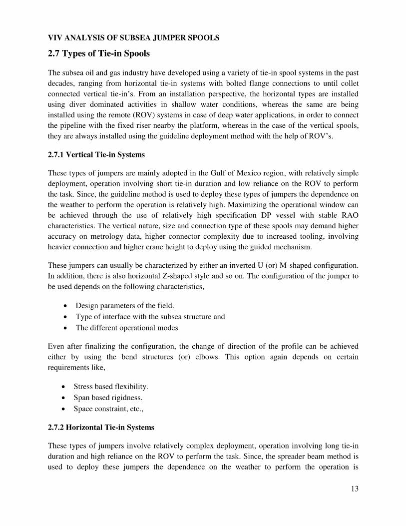
The various steps involved in the installation of the horizontal jumper are listed below,
The horizontal tie-in system is hooked up to a spreader beam and then it is deployed, to
until it is lowered up to a few meters above the target area seabed as shown in figure 8.
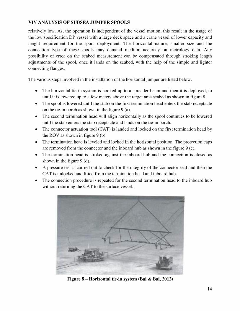
The spool is lowered until the stab on the first termination head enters the stab receptacle
on the tie-in porch as shown in the figure 9 (a).
The second termination head will align horizontally as the spool continues to be lowered
until the stab enters the stab receptacle and lands on the tie-in porch.
The connector actuation tool (CAT) is landed and locked on the first termination head by
the ROV as shown in figure 9 (b).
The termination head is leveled and locked in the horizontal position. The protection caps
are removed from the connector and the inboard hub as shown in the figure 9 (c).
The termination head is stroked against the inboard hub and the connection is closed as
shown in the figure 9 (d).
A pressure test is carried out to check for the integrity of the connector seal and then the
CAT is unlocked and lifted from the termination head and inboard hub.
The connection procedure is repeated for the second termination head to the inboard hub
without returning the CAT to the surface vessel.
Figure 8 – Horizontal tie-in system (Bai & Bai, 2012)
VIV ANALYSIS OF SUBSEA JUMPER SPOOLS
15
Figure 9 – Sequence of installation for horizontal tie-in system (Bai & Bai, 2012)
Thus, this chapter has provided an insight into the usage based classification of the pipelines,
their design requirements and the different pipeline installation methods available. Even though,
we understand from this chapter that, the installation limitations of the pipeline have introduced
the use of the tie-in spools, their design requirements are mainly the pipeline thermal expansion
and the pipeline installation inaccuracy data. This chapter has also provided information about
the types of tie-in spools available and a comparison between them to understand the case
specific use of the type.
VIV ANALYSIS OF SUBSEA JUMPER SPOOLS
16
CHAPTER 3
VIV PHENOMENON
3.1 Vortex Formation
Whenever a structure is introduced into a flowing medium, it disturbs the regular (undisturbed)
medium flow as an obstacle along its path. This makes the medium to exert some force on the
structure based on the water particle velocity and acceleration. Just like the fluid force, the
structure will also exert an equal and opposite force to the fluid. The level of the resistive force
and the impact made by the fluid force on the structure depends on the material strength of the
structure. For a structure with light weight material of construction, the resistance to the applied
force will be less and eventually they deform more compared with the structures that are made of
heavy material. As they deform they change their orientation with respect to the fluid medium
resulting in different magnitude of force acting on them. On the other hand when the structure
resistive force is high enough to the fluid exerted force, then it results in the generation of
stronger wakes on the downstream side. The phase and pattern of generation of these wakes
depends on the fluid characteristics under consideration and also to some extent on the
considered structure roughness. These wakes (vortices) formed on the downstream will generate
low pressure zone on the side of the vortex formation and tend the structure to oscillate (vibrate)
based on the flow of energy principle from high pressure to low pressure. These are termed as
Vortex Induced Vibrations (VIV). These vibrations are usually considered as the secondary
design load conditions with the life condition of up to least until damage has been made. With
the progress of the oil discovery to remote, harsh and deep water depths, the installation
limitations influence the engineers to utilize the maximum material limit of the structure, making
them more lighter, flexible and more prone to vortex induced vibrations.
3.1.1 Factors Influencing Vortex Induced Vibrations
The occurrence and level of impact due to the vortex induced vibrations depends on the
following factors,
Upstream fluid characteristics
Fluid-Structure interface criterions and
Structural properties
3.1.2 Physics behind Vortex Formation
When the fluid particles flow from a free stream towards the leading edge of the stationary
structure (in our case it is the jumper cylinder), its pressure will develop from its free stream
pressure to its stagnation pressure. This high pressure of the fluid particle will impel the fluid to
VIV ANALYSIS OF SUBSEA JUMPER SPOOLS
17
flow across the cylinder forming a boundary layer zone on the fluid cylinder interface, as a result
of the viscous friction. Normally, the velocity profile on the boundary layer will increase
gradually from zero at the contact point to until upstream free flow velocity far away from the
boundary layer the fluid is usually treated as in-viscid at this region (Prandtl, 1904). This
distribution of velocity intensity depends on the boundary layer thickness which depends on the
viscosity of the fluid involved. As the viscosity increases, the boundary layer becomes thicker.
The boundary layer usually tends to develop along the transverse length (x) of the fluid flow and
is usually a function proportional to √x. The boundary layer thickness is the distance normal to
the fluid flow from the point of contact to until the flow velocity would be 99% of the upstream
undisturbed free stream velocity (Newman, 1977). This is given in the equation 3.1.2, = . …………… . . .
Here, = ℎ ℎ ℎ
= ℎ
However, the pressure developed based on the upstream free stream velocity is not high enough
to get the flow to until the back of the cylinder forming a complete boundary zone even at high
Reynolds number condition. Thus, the flow starts to separate from the cylinder at the widest
possible section of the cylinder (Blevins, 2001). This sheared flow of the fluid will have two
different velocity zones once it is sheared off, one near the cylinder shear off point where the
velocity is less and another one at a distance from the sheared off flow along the stream behind
the cylinder where the velocity is much higher compared to the former. This difference in
velocity makes the vortices on the downstream to swirl and form vortices and circulation into
large discrete vortices which form alternatively on opposite sides of the considered cylinder
(Perry, Chong & Lim (1982), Williamson & Roshko, (1988)). At one certain stage of this vortex
development on the downstream, the strength of the vortex becomes sufficiently large to pull the
opposite sided vortex to shed from the cylinder. From then the increase in strength of the vortices
stops as it get utilized for vortices shedding further and the phenomenon of vortex shedding on
the downstream continues alternatively (Kenny, 1993).
3.1.3 Factors Influencing Vortices Intensity
Based on the vortex formation physics, the main characteristics determining the vortex intensity
and their pattern of formation on the downstream are,
Velocity of the fluid (defining the free stream pressure)
Viscosity of the fluid (defining the differential velocity)

VIV ANALYSIS OF SUBSEA JUMPER SPOOLS
18
Diameter of the cylinder (defining both the stagnation pressure impact, resistive force and
the differential pressure)
Cylinder roughness (defining the differential pressure)
3.2 Parameters to define the vortex significance
There are three categories of parameters that are used to define the significance of the vortex
being shed on the downstream. They are,
i. Fluid Parameters
ii. Fluid-Structure Interface (FSI) Parameters and
iii. Structure Parameters
The individual parameters and their influence on vortices intensities are detailed in the following
sections.
3.2.1 Fluid Parameters
The parameters that involve the properties and characteristics of the upstream fluid medium
which can impact change on the vortex shedding on the downstream are included under this.
3.2.1.1 Reynolds Number (Re)
The parameter that relates the first three vortex intensity characteristics in section 3.1.3 being the
Reynolds number, which helps in describing the flow pattern under various flow conditions for a
steady flow with similar streamlines around the cylinder (Schlichting, 1968).The expression is
given in equation 3.2.1.1,
= = ∗ ……………… . . .
Here, = ℎ
= ℎ
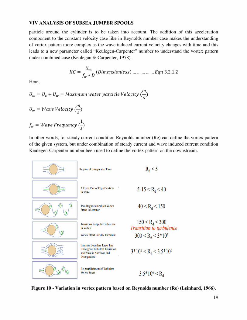
The difference in the vortex pattern as a function of the Reynolds number is represented in the
figure 10.
3.2.1.2 Keulegen-Carpenter Number (KC)
If the system is exposed to a harmonic oscillating flow (i.e., waves) then the influence of the
added mass on the vortex shedding pattern of the system due to the acceleration of the fluid
VIV ANALYSIS OF SUBSEA JUMPER SPOOLS
19
particle around the cylinder is to be taken into account. The addition of this acceleration
component to the constant velocity case like in Reynolds number case makes the understanding
of vortex pattern more complex as the wave induced current velocity changes with time and this
leads to a new parameter called “Keulegen-Carpenter” number to understand the vortex pattern
under combined case (Keulegan & Carpenter, 1958).
= ∗ …………… . . .
Here, = + =
=
=
In other words, for steady current condition Reynolds number (Re) can define the vortex pattern
of the given system, but under combination of steady current and wave induced current condition
Keulegen-Carpenter number been used to define the vortex pattern on the downstream.
Figure 10 - Variation in vortex pattern based on Reynolds number (Re) (Leinhard, 1966).
VIV ANALYSIS OF SUBSEA JUMPER SPOOLS
20
3.2.1.3 Current Flow Velocity ratio
In a real sea state, it is not just either wave or current scenario it is always a combination of both.
But, in our area of concern near the seabed, the level of wave influence over the current
gradually decreases, while moving from a shallow water case to that of ultra-deep water. This
current-wave percentage of influence in a considered environment can be determined based on
the “Current Flow Velocity” ratio.
= + …………… . . .
3.2.1.4 Turbulence Intensity
Any fluctuation from the mean fluid flow velocity under considered environmental conditions is
defined by the turbulence intensity and is represented by the equation 3.2.1.4,
= …………… . . .
Here, = = −
=
3.2.1.5 Shear Fraction of Flow Profile
The amount of shear in the considered non-uniform fluctuating current profile is usually
represented as a fraction to that of the mean velocity case and is defined by the equation 3.2.1.5,
ℎ = ∆ …………… . . . .
Here, ∆ = ℎ = − �
� = ℎ
3.2.2 Fluid Structure Interface (FSI) Parameters
Those parameters that define the structural response due to the variation in shedding pattern
based on the Fluid Structure Interface (FSI) are listed below.
VIV ANALYSIS OF SUBSEA JUMPER SPOOLS
21
3.2.2.1 Reduced Velocity
Based on the environmental scenario involved, either it is steady current or a combination of
steady current and time dependent wave induced current, the vortices generated on the
downstream will influence the system to oscillate based on the differential pressure zone. The
velocity at which the vortices are shed on the downstream induce vibration on the system is
given by the “Reduced Velocity”. This vibration amplitude path length per cycle of oscillation for the given model conditions is given by equation 3.2.2.1 (a) (DNV-RP-F105, 2006).
= ∗ …………… . . .
Here,
= ℎ ( )
The equation 3.2.2.1 (a) makes it clear that in additional to the environmental condition the
amplitude of oscillation attains its maximum (critical) state, when the frequency of vibration
matches with the natural frequency. This natural frequency of the system depends on the system
stiffness, end support conditions, unsupported span length and effective mass of the system. It is
represented by equation 3.2.2.1 (b),
= √ ∗∗ ( )…………… . . .
Here, = = . − = . − = . −
= ( ) = = ( − � ) = ( )
VIV ANALYSIS OF SUBSEA JUMPER SPOOLS
22
= + +
= ( )
= ( )
= ℎ ( ) = ℎ ℎ
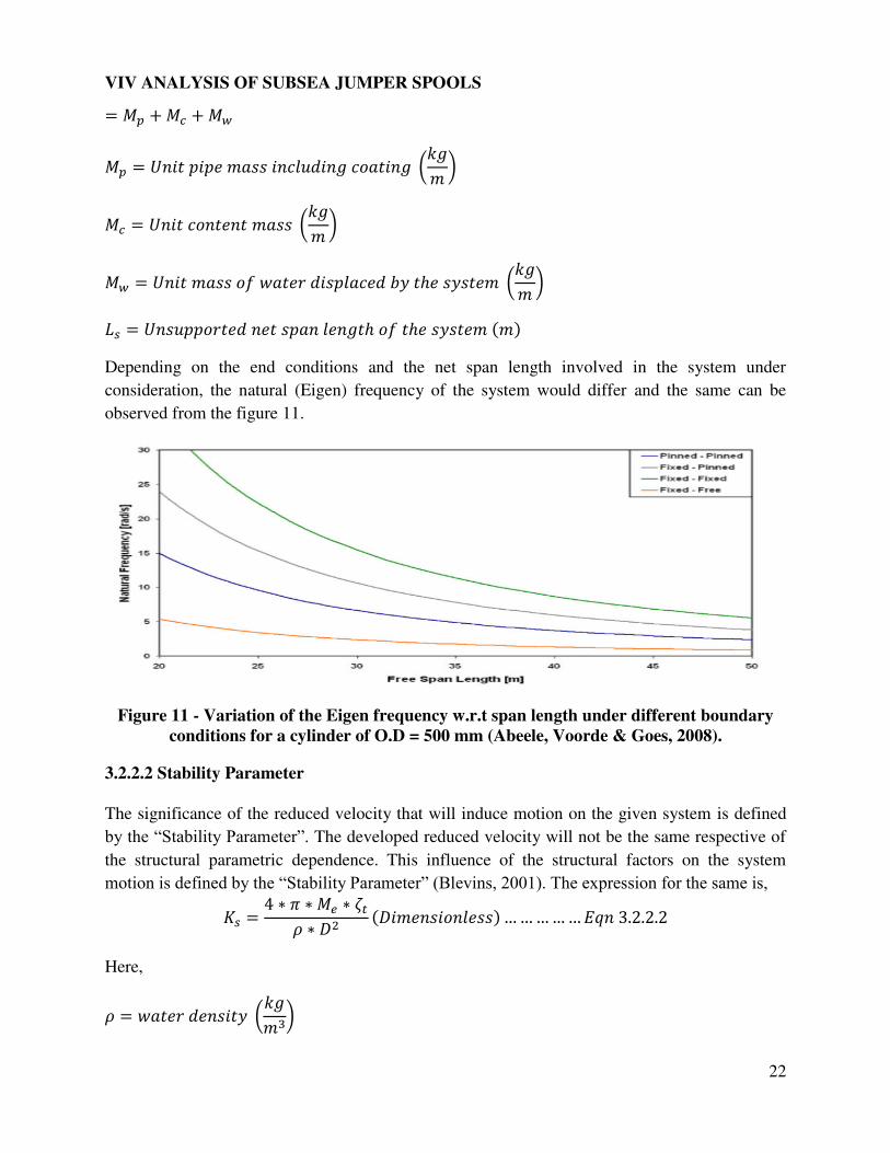
Depending on the end conditions and the net span length involved in the system under
consideration, the natural (Eigen) frequency of the system would differ and the same can be
observed from the figure 11.
Figure 11 - Variation of the Eigen frequency w.r.t span length under different boundary
conditions for a cylinder of O.D = 500 mm (Abeele, Voorde & Goes, 2008).
3.2.2.2 Stability Parameter
The significance of the reduced velocity that will induce motion on the given system is defined
by the “Stability Parameter”. The developed reduced velocity will not be the same respective of
the structural parametric dependence. This influence of the structural factors on the system
motion is defined by the “Stability Parameter” (Blevins, 2001). The expression for the same is, = ∗ ∗ ∗∗ …………… . . .
Here,
= ( )
VIV ANALYSIS OF SUBSEA JUMPER SPOOLS
23
= = + � + ℎ = = . ℎ = . − . ℎ
� =
ℎ =
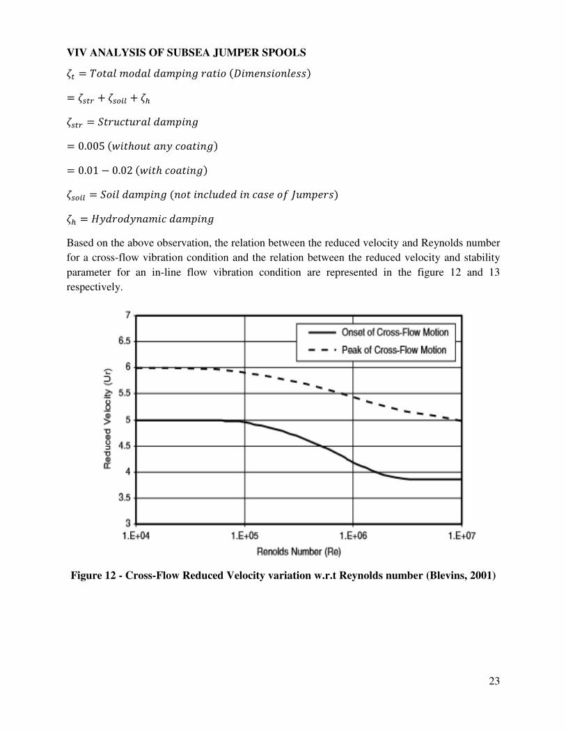
Based on the above observation, the relation between the reduced velocity and Reynolds number
for a cross-flow vibration condition and the relation between the reduced velocity and stability
parameter for an in-line flow vibration condition are represented in the figure 12 and 13
respectively.
Figure 12 - Cross-Flow Reduced Velocity variation w.r.t Reynolds number (Blevins, 2001)
VIV ANALYSIS OF SUBSEA JUMPER SPOOLS
24
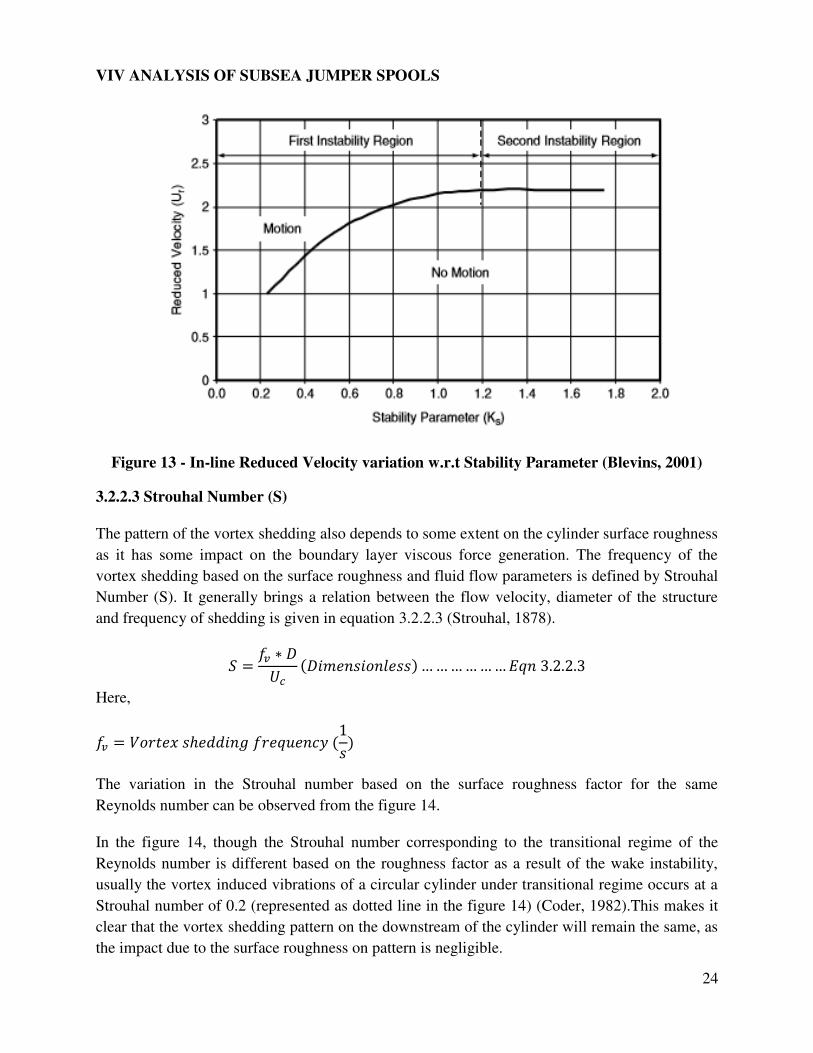
Figure 13 - In-line Reduced Velocity variation w.r.t Stability Parameter (Blevins, 2001)
3.2.2.3 Strouhal Number (S)
The pattern of the vortex shedding also depends to some extent on the cylinder surface roughness
as it has some impact on the boundary layer viscous force generation. The frequency of the
vortex shedding based on the surface roughness and fluid flow parameters is defined by Strouhal
Number (S). It generally brings a relation between the flow velocity, diameter of the structure
and frequency of shedding is given in equation 3.2.2.3 (Strouhal, 1878).
= ∗ ……………… . . .
Here,
= ℎ
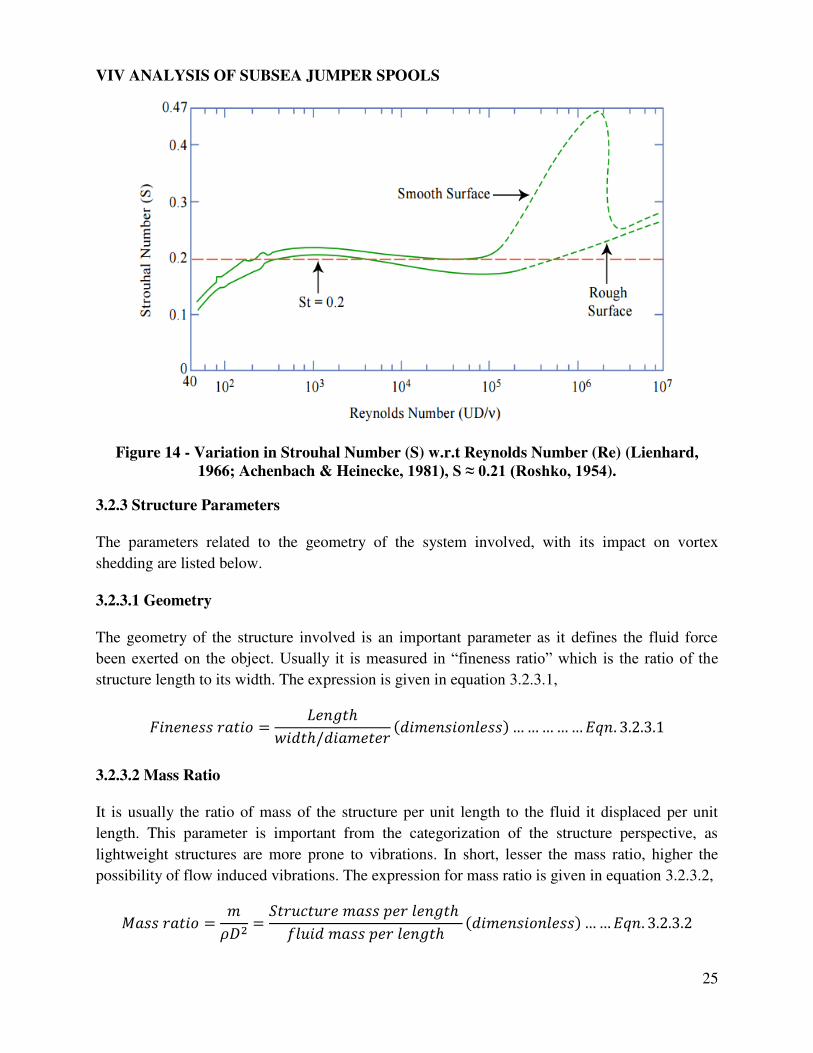
The variation in the Strouhal number based on the surface roughness factor for the same
Reynolds number can be observed from the figure 14.
In the figure 14, though the Strouhal number corresponding to the transitional regime of the
Reynolds number is different based on the roughness factor as a result of the wake instability,
usually the vortex induced vibrations of a circular cylinder under transitional regime occurs at a
Strouhal number of 0.2 (represented as dotted line in the figure 14) (Coder, 1982).This makes it
clear that the vortex shedding pattern on the downstream of the cylinder will remain the same, as
the impact due to the surface roughness on pattern is negligible.
VIV ANALYSIS OF SUBSEA JUMPER SPOOLS
25
Figure 14 - Variation in Strouhal Number (S) w.r.t Reynolds Number (Re) (Lienhard,
1966; Achenbach & Heinecke, 1981), S ≈ 0.21 (Roshko, 1954).
3.2.3 Structure Parameters
The parameters related to the geometry of the system involved, with its impact on vortex
shedding are listed below.
3.2.3.1 Geometry
The geometry of the structure involved is an important parameter as it defines the fluid force
been exerted on the object. Usually it is measured in “fineness ratio” which is the ratio of the
structure length to its width. The expression is given in equation 3.2.3.1,
= ℎℎ/ …………… . . . .
3.2.3.2 Mass Ratio
It is usually the ratio of mass of the structure per unit length to the fluid it displaced per unit
length. This parameter is important from the categorization of the structure perspective, as
lightweight structures are more prone to vibrations. In short, lesser the mass ratio, higher the
possibility of flow induced vibrations. The expression for mass ratio is given in equation 3.2.3.2,
= = ℎ ℎ …… . . . .
VIV ANALYSIS OF SUBSEA JUMPER SPOOLS
26
3.2.3.3 Damping Factor
It is usually the ratio of the energy dissipated by the structure upon oscillations induced by the
vortices to the energy imposed by the fluid upon the structure. It is usually expressed in multiples
of the critical damping factor. If the energy imposed by the fluid on the structure is less than the
energy it has expended in damping, then the structure will eventually diminish oscillations. The
expression of it is given in equation 3.2.3.3,
= ∗ ℎ …………… . . . .
3.3 “Lock-in” Phenomenon
As the system starts to vibrate at a specified frequency and amplitude based on the reduced
velocity condition in the initial stage, its Eigen frequency alters due to the change in the system
effective mass based on the added mass difference. This Eigen frequency difference is
compensated by the change in the vibration frequency of the system which has control over the
shedding frequency. When this vibration frequency becomes near, equal or multiples of the
stationary shedding frequency, then it results in a critical phenomenon of importance called the
“Lock-in” (Blevins, 2001).
Usually every system has a range of reduced velocity for which it has the ability to adjust its
Eigen frequency with control over the shedding frequency based on vibration frequency
compensation. This range within which the system vibration frequency has the control over the
shedding frequency is called the “Lock-in Range”.
The phenomenon of “Lock-in” can be mathematically expressed as follows,
The Eigen frequency of the system in terms of reduced velocity is given by,
= ∗ …………… .
The shedding frequency of the system in terms of stationary Strouhal number is given by,
= ∗ …………… .
Under the condition of the vibration frequency with control over the shedding frequency the
equations 3.3 (a) and (b) are related by,
VIV ANALYSIS OF SUBSEA JUMPER SPOOLS
27
≅ ∗ = ∗ => = …………… .
Based on the section 3.2.2.3 input that, vortex induced vibrations for a transitional regime starts
around a Strouhal number of 0.2, the reduced velocity corresponding to the onset of the lock-in
range will be around 5. But, there are also low frequency regions where this lock-in phenomenon
can be observed when the vibration frequency is a sub-multiple of the stationary shedding
frequency.
3.4 Types of Vortex Induced Vibrations
The two types of vortex induced motions the system gets exposed to based on the direction of
fluid attack relative to the cylindrical axis are,
In-line VIV
Cross-Flow VIV
3.4.1 In-line VIV
When the vibration induced in the system for a given modal shape based on the vortex shedding
pattern, is translational and along the direction of the fluid attack is defined as “In-line” VIV (Carruth & Cerkovnik, 2007).
Though the amplitude involved in this type of oscillations is only 10% of that in case of cross-
flow oscillations due to the force components difference (Guo et al., 2005), these oscillations
will take place at a lower vibration frequency than that of the critical frequency in the cross-flow
condition. Usually, the system will start to oscillate along the flow direction when the vibration
frequency is 1/3rd
of its Eigen frequency. The expression for the same is given in equation 3.4.1,
= …………… . . .
This in-line oscillation frequency gradually increase with increase in the reduced velocity (The
theory behind is explained in section the 3.5 in this chapter) and it will reach the lock-in
condition when the vibration frequency is one-half of the Eigen frequency.
The first two modes of instability under this type of oscillation have their maximum amplitude
response at a reduced velocity of 1.9 and 2.6 respectively and the possibility to prevent them will
be by maintaining the stability parameter above 1.8 (Wootton, 1991).
VIV ANALYSIS OF SUBSEA JUMPER SPOOLS
28
The amplitude response corresponding to a reduced velocity of less than 2.2 makes the shedding
remain symmetric and on the other hand for a reduced velocity above 2.2 the shedding changes
into alternate type.
3.4.2 Cross-Flow VIV
When the vibration induced in the system for a given modal shape based on the vortex shedding
pattern is in two different translational directions and being perpendicular to that of the fluid
attack, then it is defined as “Cross-Flow” VIV (Carruth & Cerkovnik, 2007).
Since, these oscillations take place at a vibration frequency much higher than that of the in-line
oscillation case, though the amplitude associated are high, these cannot turn into the governing
criterion for design in our case as the span length is limited for jumpers. This type of oscillations
approach lock-in phenomenon as the vibration frequency is near, equal to (or) multiple of the
Eigen frequency.
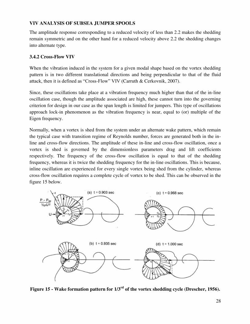
Normally, when a vortex is shed from the system under an alternate wake pattern, which remain
the typical case with transition regime of Reynolds number, forces are generated both in the in-
line and cross-flow directions. The amplitude of these in-line and cross-flow oscillation, once a
vortex is shed is governed by the dimensionless parameters drag and lift coefficients
respectively. The frequency of the cross-flow oscillation is equal to that of the shedding
frequency, whereas it is twice the shedding frequency for the in-line oscillations. This is because,
inline oscillation are experienced for every single vortex being shed from the cylinder, whereas
cross-flow oscillation requires a complete cycle of vortex to be shed. This can be observed in the
figure 15 below.
Figure 15 - Wake formation pattern for 1/3rd
of the vortex shedding cycle (Drescher, 1956).
VIV ANALYSIS OF SUBSEA JUMPER SPOOLS
29
Usually systems tend to trace an “8” shaped motion due to vortex induced vibrations (Jauvtis &
Williamson, 2003). Under fully developed vortex shed pattern condition, the amplitude of the
cross-flow oscillations are much higher when compared to that of the in-line oscillations, but the
average force for the cross-flow oscillations are zero as they tend to experience the lift force
about the centre of flow to the system, whereas it is not the case for the in-line oscillations, the
average force of drag is not zero as it always needs some resistive force against the fluid flow
force and the frequency of oscillation is also twice in case of drag when compared to that of the
lift forces. .
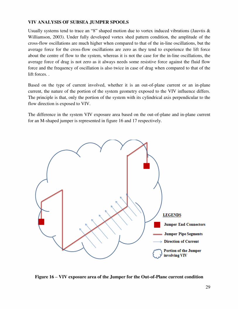
Based on the type of current involved, whether it is an out-of-plane current or an in-plane
current, the nature of the portion of the system geometry exposed to the VIV influence differs.
The principle is that, only the portion of the system with its cylindrical axis perpendicular to the
flow direction is exposed to VIV.
The difference in the system VIV exposure area based on the out-of-plane and in-plane current
for an M-shaped jumper is represented in figure 16 and 17 respectively.
Figure 16 – VIV exposure area of the Jumper for the Out-of-Plane current condition
VIV ANALYSIS OF SUBSEA JUMPER SPOOLS
30
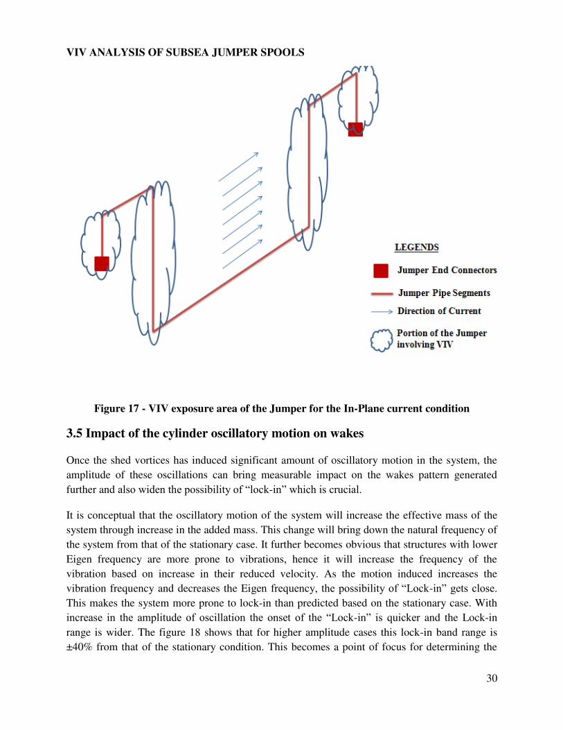
Figure 17 - VIV exposure area of the Jumper for the In-Plane current condition
3.5 Impact of the cylinder oscillatory motion on wakes
Once the shed vortices has induced significant amount of oscillatory motion in the system, the
amplitude of these oscillations can bring measurable impact on the wakes pattern generated
further and also widen the possibility of “lock-in” which is crucial.
It is conceptual that the oscillatory motion of the system will increase the effective mass of the
system through increase in the added mass. This change will bring down the natural frequency of
the system from that of the stationary case. It further becomes obvious that structures with lower
Eigen frequency are more prone to vibrations, hence it will increase the frequency of the
vibration based on increase in their reduced velocity. As the motion induced increases the
vibration frequency and decreases the Eigen frequency, the possibility of “Lock-in” gets close. This makes the system more prone to lock-in than predicted based on the stationary case. With
increase in the amplitude of oscillation the onset of the “Lock-in” is quicker and the Lock-in
range is wider. The figure 18 shows that for higher amplitude cases this lock-in band range is
±40% from that of the stationary condition. This becomes a point of focus for determining the
VIV ANALYSIS OF SUBSEA JUMPER SPOOLS
31
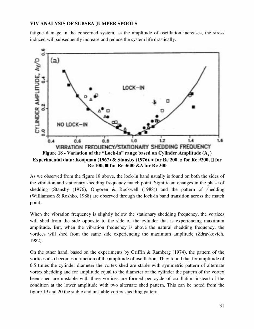
fatigue damage in the concerned system, as the amplitude of oscillation increases, the stress
induced will subsequently increase and reduce the system life drastically.
Figure 18 - Variation of the “Lock-in” range based on Cylinder Amplitude (��
Experimental data: Koopman (1967) & Stansby (1976), for Re 200, for Re 9200, for
Re 100, for Re 3600 &Δ for Re 300
As we observed from the figure 18 above, the lock-in band usually is found on both the sides of
the vibration and stationary shedding frequency match point. Significant changes in the phase of
shedding (Stansby (1976), Ongoren & Rockwell (1988)) and the pattern of shedding
(Williamson & Roshko, 1988) are observed through the lock-in band transition across the match
point.
When the vibration frequency is slightly below the stationary shedding frequency, the vortices
will shed from the side opposite to the side of the cylinder that is experiencing maximum
amplitude. But, when the vibration frequency is above the natural shedding frequency, the
vortices will shed from the same side experiencing the maximum amplitude (Zdravkovich,
1982).
On the other hand, based on the experiments by Griffin & Ramberg (1974), the pattern of the
vortices also becomes a function of the amplitude of oscillation. They found that for amplitude of
0.5 times the cylinder diameter the vortex shed are stable with symmetric pattern of alternate
vortex shedding and for amplitude equal to the diameter of the cylinder the pattern of the vortex
been shed are unstable with three vortices are formed per cycle of oscillation instead of the
condition at the lower amplitude with two alternate shed pattern. This can be noted from the
figure 19 and 20 the stable and unstable vortex shedding pattern.
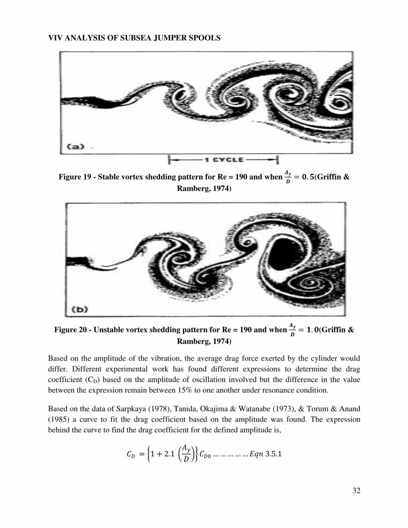
VIV ANALYSIS OF SUBSEA JUMPER SPOOLS
32
Figure 19 - Stable vortex shedding pattern for Re = 190 and when ��� = . �(Griffin &
Ramberg, 1974)
Figure 20 - Unstable vortex shedding pattern for Re = 190 and when ��� = . (Griffin &
Ramberg, 1974)
Based on the amplitude of the vibration, the average drag force exerted by the cylinder would
differ. Different experimental work has found different expressions to determine the drag
coefficient (CD) based on the amplitude of oscillation involved but the difference in the value
between the expression remain between 15% to one another under resonance condition.
Based on the data of Sarpkaya (1978), Tanida, Okajima & Watanabe (1973), & Torum & Anand
(1985) a curve to fit the drag coefficient based on the amplitude was found. The expression
behind the curve to find the drag coefficient for the defined amplitude is,
= { + . (� )} …………… . .
VIV ANALYSIS OF SUBSEA JUMPER SPOOLS
33
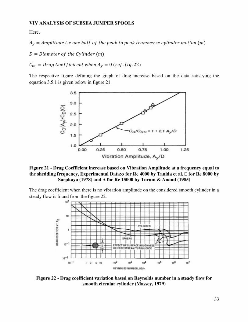
Here, � = � . ℎ ℎ = ℎ = ℎ � = . .
The respective figure defining the graph of drag increase based on the data satisfying the
equation 3.5.1 is given below in figure 21.
Figure 21 - Drag Coefficient increase based on Vibration Amplitude at a frequency equal to
the shedding frequency, Experimental Data: for Re 4000 by Tanida et al, for Re 8000 by
Sarpkaya (1978) and Δ for Re 15000 by Torum & Anand (1985)
The drag coefficient when there is no vibration amplitude on the considered smooth cylinder in a
steady flow is found from the figure 22.
Figure 22 - Drag coefficient variation based on Reynolds number in a steady flow for
smooth circular cylinder (Massey, 1979)
VIV ANALYSIS OF SUBSEA JUMPER SPOOLS
34
Vandiver (1983) found that the drag experienced marine cables vibrating due to vortex shedding
can be predicted using the formula 3.5.2.
= { + . ( ∗ � ) . } …………… . .
Here, � = ℎ ℎ �
Whereas, Skop, Griffin & Ramberg (1977), found another expression for the same drag increase
prediction based on his finding as represented in equation 3.5.3.
= { + . { ( + ∗ � ) ∗ [ ] − } . } …………… . .
The interesting fact between all the above three equations (Eqn. 3.5.1, 3.5.2 and 3.5.3) is that at
the resonance condition the difference in the drag coefficient outcome from individual case study
doesn’t deviate from the other by more than 15%.
Based on the value of drag coefficient determined through the expression for the considered
condition of vibration, the average drag force per unit length acting on the system is given by,
= ( )…………… . . .
Here,
= ℎ
=
Thus, the impact of the system vibration oscillation on further generation of wakes has the
following effects,
i. Increase the strength of the vortices based on higher separation force and enhanced
velocity of separation (Davies (1976), Griffin & Ramberg (1974)).
ii. Cause the vibration frequency to shift towards the stationary shedding frequency (Bishop
& Hassan (1964)), increasing the possibility of lock-in phenomenon with widening of
lock-in band based on the amplitude of oscillation involved.
iii. It alters the phase, sequence and pattern of the vortex generated based on the amplitude
(Zdravkovich (1982), Ongoren & Rockwell (1988), Williamson & Roshko (1988)).
VIV ANALYSIS OF SUBSEA JUMPER SPOOLS
35
iv. Increases the mean drag force acting on the system based on drag coefficient increase
with respect to the amplitude (Bishop & Hassan (1964), Tanida et al., (1973), Sarpkaya
(1978)).
3.6 VIV Mitigation
The consequences of the “Lock-in” phenomenon, like the magnification of the amplitude of vibration and the drag force experienced by the system can be suppressed by modifying either
the structure (or) the flow associated with the system (Blevins, 2001).
3.6.1 Increased Stability Parameter
As we observe from the fig. 13 above, that any increase in the stability parameter will increase
the requirement of the reduced velocity for the system to fall in the “lock-in” zone. This increase in the stability parameter of the system can be achieved through either increasing the effective
unit mass of the system (or) increasing the total modal damping ratio (see equation 3.2.2.2). Both
of these possibilities can be achieved only through the material parameter of the structure, as all
the other associated parameters of the system remains fixed. Use of other materials such as
viscoelastic, rubber and wood with high internal damping (or) any external damping devices will
help to achieve increased stability parameter. In particular, if the stability parameter exceeds
about a specific value, then the associated amplitude of resonance will be less than 1% of the
system diameter, this can usually be neglected in comparison to the drag force experienced by
the system (Blevins, 2001).
3.6.2 Avoiding Resonance
Resonance possibility can be avoided by maintaining the reduced velocity (See equation 3.2.2.1
(a)) of the system less than 1. From the equation 3.2.2.1 (a), we can observe that except for the
Eigen frequency of the system all other parameters remain fixed. Therefore, the reduction in the
reduced velocity is possible only through increasing the Eigen frequency of the system. System
with higher Eigen frequency means that the system is rigid. Therefore, the increase in the Eigen
frequency requires proper stiffening of the system through improving the rigidity of the system
configuration. This is the most practical case for the slender structures (Blevins, 2001).
3.6.3 Streamline Cross Section
Once the flow separation from the structure at the downstream is decreased, then the intensity of
the vortices that are shed gets reduced, this in turn reduces the drag force experienced by the
system. Streamlining the vortices on the downstream of a structure normally requires a taper of 6
longitudinal for every unit lateral (or) an included angle of the taper not more than 8-10 degrees.
This method of streamlining the structure downstream would be effective in the cases with fixed
VIV ANALYSIS OF SUBSEA JUMPER SPOOLS
36
direction of current flow relative to the system that has sufficient rigidity in order to avoid any
further fluttering (Blevins, 2001).
3.6.4 Add a Vortex Suppression Device
The physics behind these vortex suppression devices is that, they interrupt the proper boundary
layer formation in the generation of an organized, two dimensional vortex streets on the
downstream of the system. This is usually achieved through the introduction of an artificial
turbulence on the downstream (Blevins, 2001).
From this chapter, we understood the physics behind the vortex shedding phenomenon, the
factors that influence their generation, the factors that can alter the intensity of the vortices
formed & the parameters that can be used to quantify those intensities. It also helps to understand
the most crucial part of the vortex shedding, the “Lock-in” phenomenon & also the severity the system would face with a further wakes generation during resonance. Furthermore, it also
explains the types of oscillations that the system will experience, their range of occurrence &
also the possible ways to suppress them.
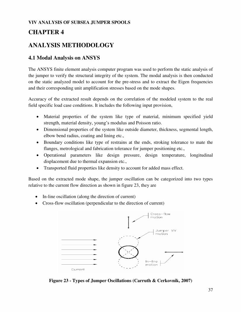
VIV ANALYSIS OF SUBSEA JUMPER SPOOLS
37
CHAPTER 4
ANALYSIS METHODOLOGY
4.1 Modal Analysis on ANSYS
The ANSYS finite element analysis computer program was used to perform the static analysis of
the jumper to verify the structural integrity of the system. The modal analysis is then conducted
on the static analyzed model to account for the pre-stress and to extract the Eigen frequencies
and their corresponding unit amplification stresses based on the mode shapes.
Accuracy of the extracted result depends on the correlation of the modeled system to the real
field specific load case conditions. It includes the following input provision,
Material properties of the system like type of material, minimum specified yield
strength, material density, young’s modulus and Poisson ratio.
Dimensional properties of the system like outside diameter, thickness, segmental length,
elbow bend radius, coating and lining etc.,
Boundary conditions like type of restrains at the ends, stroking tolerance to mate the
flanges, metrological and fabrication tolerance for jumper positioning etc.,
Operational parameters like design pressure, design temperature, longitudinal
displacement due to thermal expansion etc.,
Transported fluid properties like density to account for added mass effect.
Based on the extracted mode shape, the jumper oscillation can be categorized into two types
relative to the current flow direction as shown in figure 23, they are
In-line oscillation (along the direction of current)
Cross-flow oscillation (perpendicular to the direction of current)
Figure 23 - Types of Jumper Oscillations (Carruth & Cerkovnik, 2007)
VIV ANALYSIS OF SUBSEA JUMPER SPOOLS
38
4.2 VIV Analysis
In addition to the above list of inputs to perform the modal analysis in ANSYS, the following
inputs are also required for a complete VIV analysis of the system.
Environmental data like significant wave height, wave period, current velocity at the sea
surface, wave and current heading relative to the system.
Seabed bathymetry details.
Water depth of operation involved.
4.2.1 Environmental Modeling
As specified in section.3 of DNV-RP-F105, the environment to which the jumper system is
exposed to, be modeled based on a return period of 100 year with a long term distribution
statistics both for the steady state current and wave induced velocity and period of oscillation at
the pipe level. The characteristics of the current and wave is usually extrapolated from the free
surface to the pipe level to study the jumper characteristics as they govern the response.
4.2.1.1 Current
The variation of the current velocity relative to the water depth is considered relative and the
total current velocity from the components of tidal and wind induced current and its variation
along the water depth from the reference surface is modeled as per section D-301 of DNV-OS-
J101.
Based on section D-301 from DNV-OS-J101, = � + � …………… . . . .
Where,
� = � (ℎ +ℎ ) / …………… . . . .
� = � (ℎ +ℎ ) − ℎ …………… . . . .
Here, = =
� =
VIV ANALYSIS OF SUBSEA JUMPER SPOOLS
39
� = ℎ = ℎ ℎ = ℎ Based on the condition mentioned in equation 4.2.1.1 (c), the equation 4.2.1.1 (a) for water
depth’s beyond η0 meters can be modified as, = � …………… . . . .
As most of the wind induced component of current for deeper cases can be contributed from the
waves with an exponential decay method.
Since, no information is available related to the intensity of current turbulence, the value is taken
as 5% as mentioned in section 3.2.12 of DNV-RP-F105.
4.2.1.2 Waves
As the intended system is exposed to the environment throughout its service life, a long term
based environmental analysis is preferred instead of the short term sea state condition. For
modeling the significant wave height (Hs) on a long term statistical basis a 3-parameter Weibull
distribution is often appropriate as per section 3.5 of DNV-RP-F105 and the Weibull distribution
is given by, = − exp − − …………… . . . .
Here, = � = + = . ℎ = . ℎ = = ℎ = =
All these Weibull distribution parameters are linked to the statistical moments (µ: mean value, σ: standard deviation, δ: skewness) as follows:
VIV ANALYSIS OF SUBSEA JUMPER SPOOLS
40
= � ( + ) + …………… . . . .
� = √� ( + ) − � ( + ) …………… . . . .
= � ∗ [ � ( + ) − � ( + ) ∗ � ( + ) + � + ]…………… . . . .
Here, � =
� = ∫ − ∗ − ∗ …………… . . . . ∞
Upon developing the equation 4.2.1.2 (a), with the assumption that = , it will result in, ln(ln( − )) = − …………… . . . .
From the above equation.4.2.1.2 (f), if we plot the histogram data from a storm of 3 hours
duration on a Weibull probability paper with as the x-axis and ln ln( − ) as the y-
axis following the alternative cumulative distribution function. The significant wave height
relative to the return period required can be obtained from the plot through extrapolation of the
plot fitted straight line which follows the Weibull distribution. The accuracy of the extrapolated
result depends on the fitness level of the plot to the Weibull distribution.
For a Weibull distributed variable the return period value (xc) is given by, = ln / + …………… . . . .
Where,
= − …………… . . . . ℎ
Here
N = number of independent events in the return period (e.g. 100 years)
This will result in the determination of the extreme sea state significant wave height for the
assumed storm duration based on the probability of exceedance considered. Once we determined
the significant wave height for the extreme sea state involved in the considered return period, its
relative time period can be obtained through the extrapolation of the linear plot fitted between
VIV ANALYSIS OF SUBSEA JUMPER SPOOLS
41
the average time periods involved for each interval of wave height recorded in the histogram
data.
Based on the Hs and Tp value of the extreme sea state for an assumed probability of exceedance
10-2
, the relative zero up-crossing period (Tz) for the peak period (Tp) can be calculated using
the relation in equation.4.2.1.2 (i),
= √ ++ …………… . . . .
Here, = ℎ . = √ .
= . − . ��√�� . < √
= √ >
From the zero up-crossing period, we can calculate the total number of waves ( observed
within the storm duration considered as shown in equation.4.2.1.2 (j),
= …………… . . . .
Based on the Gaussian process to define the surface of the sea, the corresponding highest wave
crest is given by = = � √ …………… . . . .
Here,
� = ℎ ℎ ℎ =
Based on the value of , the determination of the involved case study being
shallow/intermediate/deep water can be done through calculating the wavelength (L) using the
dispersion relation shown in equation.4.2.1.2 (l) = ∗ ∗ tanh …………… . . . .
Here,
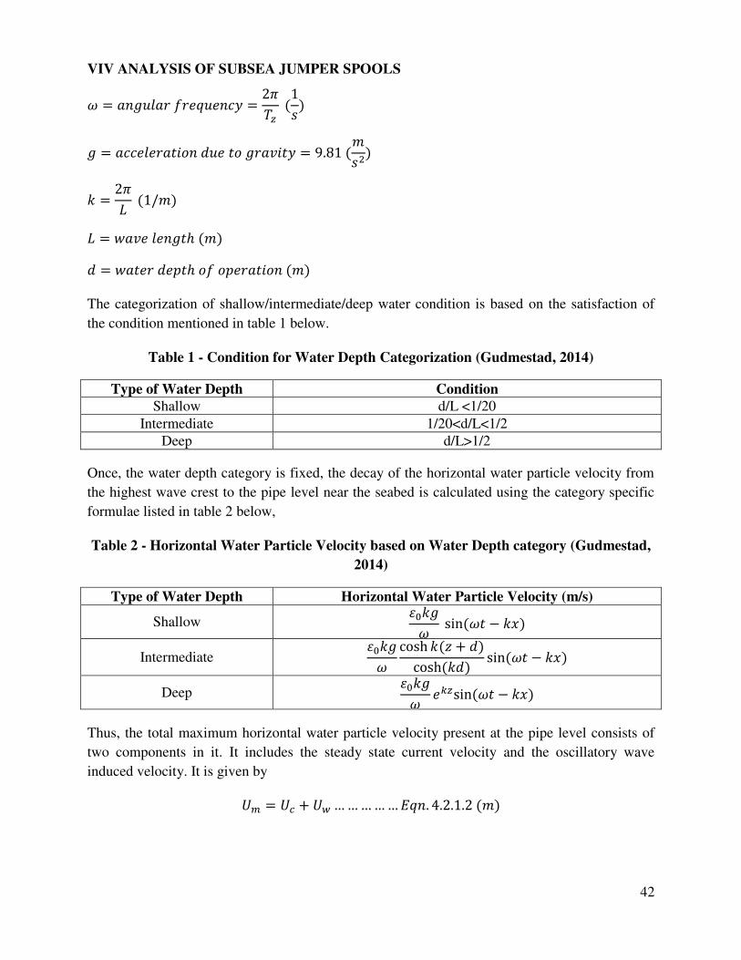
VIV ANALYSIS OF SUBSEA JUMPER SPOOLS
42
= =
= = .
= / = ℎ = ℎ
The categorization of shallow/intermediate/deep water condition is based on the satisfaction of
the condition mentioned in table 1 below.
Table 1 - Condition for Water Depth Categorization (Gudmestad, 2014)
Type of Water Depth Condition
Shallow d/L <1/20
Intermediate 1/20<d/L<1/2
Deep d/L>1/2
Once, the water depth category is fixed, the decay of the horizontal water particle velocity from
the highest wave crest to the pipe level near the seabed is calculated using the category specific
formulae listed in table 2 below,
Table 2 - Horizontal Water Particle Velocity based on Water Depth category (Gudmestad,
2014)
Type of Water Depth Horizontal Water Particle Velocity (m/s)
Shallow sin −
Intermediate cosh +cosh sin −
Deep sin −
Thus, the total maximum horizontal water particle velocity present at the pipe level consists of
two components in it. It includes the steady state current velocity and the oscillatory wave
induced velocity. It is given by = + …………… . . . .
VIV ANALYSIS OF SUBSEA JUMPER SPOOLS
43
4.2.2 Response Modeling
The amplitude response models are empirical models in agreement with the generally accepted
concept of VIV providing the maximum steady state VIV amplitude responses as a function of
the basic hydrodynamic and structural parameters mentioned and detailed in chapter.3. The
response models can possibly be generated for the following conditions
Inline VIV in steady state current and current dominated conditions.
Cross-flow VIV induced inline motion.
Cross-flow VIV in steady state current and combined wave and current conditions.
In the response models the possible two types of oscillations like the inline and cross-flow are
considered separately. But, the inline instability from the first two inline oscillation are
considered implicit, there is also a possibility of increased fatigue damage from the inline
oscillations due to the additional inline motion induced from the cross-flow oscillations under all
reduced velocity range. But, the possible potential of inline induced cross-flow oscillations are
usually neglected for reduced velocity range of 2-3. Under conditions where several modes of
the same type (either inline (or) cross-flow) are excited simultaneously then the principle of
multi-mode response shall be applicable to account the total fatigue damage.
4.2.2.1 Inline Response Modeling
The inline response model of a system free span under current dominated conditions is
associated with either alternating (or) symmetric vortex shedding and it applies for all inline
vibration modes.
The parameters that define the inline response amplitude for the concerned inline modes are
Reduced Velocity (Vr)
Stability Parameter (Ks)
Turbulence Intensity (Ic) and
Flow angle relative to the pipe ( rel)
The inline VIV induced stress range SIL is calculated using the equation 4.2.2.1 (a) below,
�� = ∗ ��� ∗ (� ) ∗ ,�� ∗ …………… . . . .
Here, ��� = � � � = .
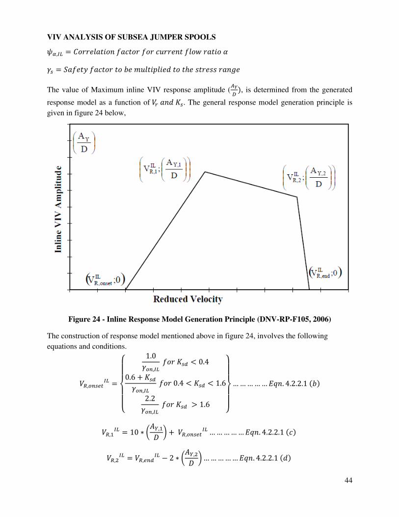
VIV ANALYSIS OF SUBSEA JUMPER SPOOLS
44
,�� = = ℎ
The value of Maximum inline VIV response amplitude (�
, is determined from the generated
response model as a function of . The general response model generation principle is
given in figure 24 below,
Figure 24 - Inline Response Model Generation Principle (DNV-RP-F105, 2006)
The construction of response model mentioned above in figure 24, involves the following
equations and conditions.
�, �� ={ . ,�� < .. +,�� . < < .. ,�� > . }
…………… . . . .
�, �� = ∗ (� , ) + �, ��…………… . . . . �, �� = �, �� − ∗ (� , )…………… . . . .
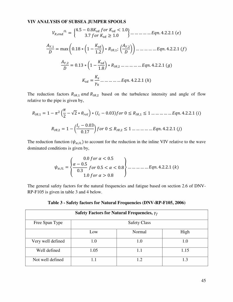
VIV ANALYSIS OF SUBSEA JUMPER SPOOLS
45
�, �� = { . − . < .. . } …………… . . . . � , = max . ∗ ( − . ) ∗ ��, ; (� , ) …………… . . . .
� , = . ∗ ( − . ) ∗ ��, …………… . . . .
= …………… . . . . ℎ
The reduction factors ��, ��, based on the turbulence intensity and angle of flow
relative to the pipe is given by,
��, = − − √ ∗ ∗ − . ��, …………… . . . .
��, = − ( − .. ) ��, …………… . . . .
The reduction function ( ,�� to account for the reduction in the inline VIV relative to the wave
dominated conditions is given by,
,�� = { . < .− .. . < < .. > . }…………… . . . .
The general safety factors for the natural frequencies and fatigue based on section 2.6 of DNV-
RP-F105 is given in table 3 and 4 below.
Table 3 - Safety factors for Natural Frequencies (DNV-RP-F105, 2006)
Safety Factors for Natural Frequencies,
Free Span Type Safety Class
Low Normal High
Very well defined 1.0 1.0 1.0
Well defined 1.05 1.1 1.15
Not well defined 1.1 1.2 1.3
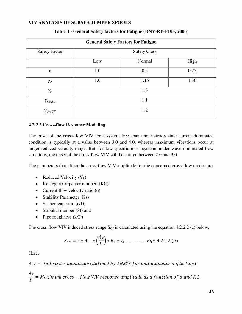
VIV ANALYSIS OF SUBSEA JUMPER SPOOLS
46
Table 4 - General Safety factors for Fatigue (DNV-RP-F105, 2006)
General Safety Factors for Fatigue
Safety Factor Safety Class
Low Normal High
1.0 0.5 0.25
1.0 1.15 1.30
1.3
,�� 1.1
, 1.2
4.2.2.2 Cross-flow Response Modeling
The onset of the cross-flow VIV for a system free span under steady state current dominated
condition is typically at a value between 3.0 and 4.0, whereas maximum vibrations occur at
larger reduced velocity range. But, for low specific mass systems under wave dominated flow
situations, the onset of the cross-flow VIV will be shifted between 2.0 and 3.0.
The parameters that affect the cross-flow VIV amplitude for the concerned cross-flow modes are,
Reduced Velocity (Vr)
Keulegan Carpenter number (KC)
Current flow velocity ratio (α) Stability Parameter (Ks)
Seabed gap ratio (e/D)
Strouhal number (St) and
Pipe roughness (k/D)
The cross-flow VIV induced stress range SCF is calculated using the equation 4.2.2.2 (a) below,
= ∗ � ∗ (� ) ∗ ∗ …………… . . . .
Here, � = � � � = − .
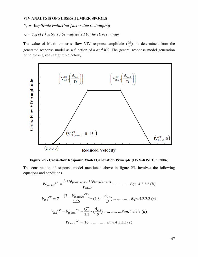
VIV ANALYSIS OF SUBSEA JUMPER SPOOLS
47
= � = ℎ
The value of Maximum cross-flow VIV response amplitude (�
, is determined from the
generated response model as a function of . The general response model generation
principle is given in figure 25 below,
Figure 25 - Cross-flow Response Model Generation Principle (DNV-RP-F105, 2006)
The construction of response model mentioned above in figure 25, involves the following
equations and conditions.
�, = ∗ �, ∗ ℎ,, …………… . . . .
�, = − − �,. ∗ . − � , …………… . . . .
�, = �, − . ∗ � , …………… . . . .
�, = …………… . . . .
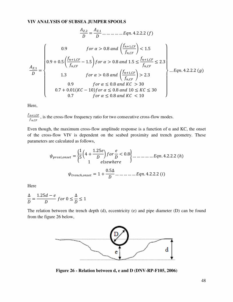
VIV ANALYSIS OF SUBSEA JUMPER SPOOLS
48
� , = � , …………… . . . .
� , ={ . > . + ,, < .. + . + ,, − . > . . + ,, .
. > . + ,, > . . . >. + . − . . . < } … . . . .
Here,
�+1,���,�� , is the cross-flow frequency ratio for two consecutive cross-flow modes.
Even though, the maximum cross-flow amplitude response is a function of α and KC, the onset
of the cross-flow VIV is dependent on the seabed proximity and trench geometry. These
parameters are calculated as follows,
�, = { ( + . ) < . ℎ }…………… . . . . ℎ
ℎ, = + . ∆…………… . . . .
Here ∆ = . − ∆
The relation between the trench depth (d), eccentricity (e) and pipe diameter (D) can be found
from the figure 26 below,
Figure 26 - Relation between d, e and D (DNV-RP-F105, 2006)
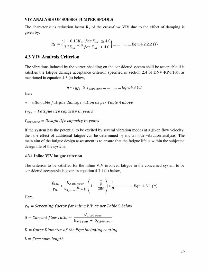
VIV ANALYSIS OF SUBSEA JUMPER SPOOLS
49
The characteristics reduction factor Rk of the cross-flow VIV due to the effect of damping is
given by,
= { − . .. − . > . }…………… . . . .
4.3 VIV Analysis Criterion
The vibrations induced by the vortex shedding on the considered system shall be acceptable if it
satisfies the fatigue damage acceptance criterion specified in section 2.4 of DNV-RP-F105, as
mentioned in equation 4.3 (a) below, ∗ � …………… . .
Here =
� = =
If the system has the potential to be excited by several vibration modes at a given flow velocity,
then the effect of additional fatigue can be determined by multi-mode vibration analysis. The
main aim of the fatigue design assessment is to ensure that the fatigue life is within the subjected
design life of the system.
4.3.1 Inline VIV fatigue criterion
The criterion to be satisfied for the inline VIV involved fatigue in the concerned system to be
considered acceptable is given in equation 4.3.1 (a) below,
,���� > , �, �� ∗ − � ∗ …………… . . .
Here,
�� =
= = , , + ,
= ℎ = ℎ
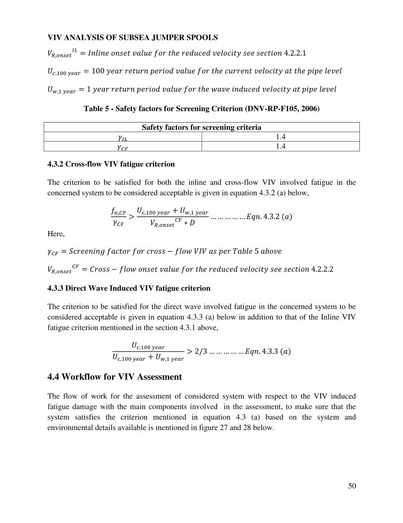
VIV ANALYSIS OF SUBSEA JUMPER SPOOLS
50
�, �� = ℎ . . .
, = ℎ ℎ
, = ℎ
Table 5 - Safety factors for Screening Criterion (DNV-RP-F105, 2006)
Safety factors for screening criteria �� 1.4
1.4
4.3.2 Cross-flow VIV fatigue criterion
The criterion to be satisfied for both the inline and cross-flow VIV involved fatigue in the
concerned system to be considered acceptable is given in equation 4.3.2 (a) below,
, > , + , �, ∗ …………… . . .
Here, = −
�, = − ℎ . . .
4.3.3 Direct Wave Induced VIV fatigue criterion
The criterion to be satisfied for the direct wave involved fatigue in the concerned system to be
considered acceptable is given in equation 4.3.3 (a) below in addition to that of the Inline VIV
fatigue criterion mentioned in the section 4.3.1 above,
, , + , > / …………… . . .
4.4 Workflow for VIV Assessment
The flow of work for the assessment of considered system with respect to the VIV induced
fatigue damage with the main components involved in the assessment, to make sure that the
system satisfies the criterion mentioned in equation 4.3 (a) based on the system and
environmental details available is mentioned in figure 27 and 28 below.
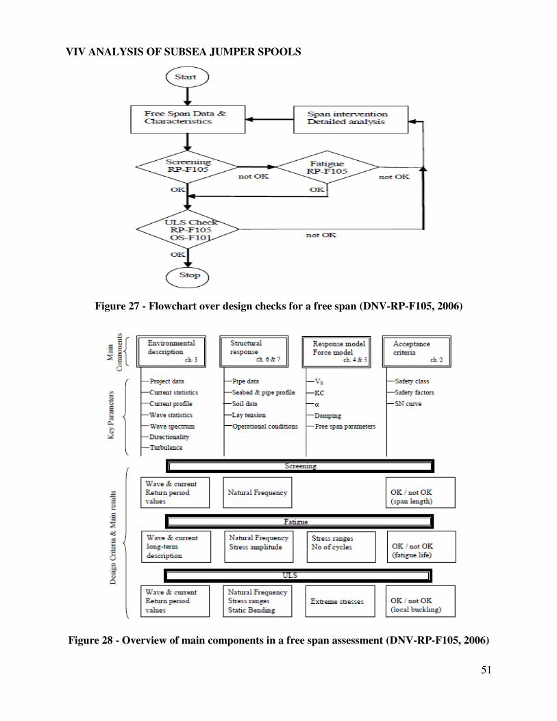
VIV ANALYSIS OF SUBSEA JUMPER SPOOLS
51
Figure 27 - Flowchart over design checks for a free span (DNV-RP-F105, 2006)
Figure 28 - Overview of main components in a free span assessment (DNV-RP-F105, 2006)
VIV ANALYSIS OF SUBSEA JUMPER SPOOLS
52
4.5 Assessment of Fatigue life
The assessment of fatigue life based on the guideline of DNV-RP-F105 as followed in this work
focus on the damage made to the design life of the system, due to the VIV when the phenomenon
of “Lock-in” happens. The damage made to the system through the vibrations that happens
before “Lock-in” has not been accounted, as the associated amplitudes are not as significant as in case of resonance.
The fatigue life of the system can be assessed based on the S-N curve method with the
assumption that the accumulated stress is linear as per Palmgren-Miner rule. When the long term
stress distribution is expressed by a stress histogram, consisting of a convenient number of
constant stress range blocks (S), each with a number of stress repetitions (ni), the accumulated
fatigue damage can then be calculated as per section.2 of DNV-RP-C203 as given in equation
4.5 (a) below,
D =∑niNi = /a�= ∗ ∑ni ∗ Simki= …………… . .
Here, = = ℎ − ℎ ℎ log = ℎ − = .
� = . ℎ �
� = . ℎ �
� = ℎ ℎ . . . . . . .
The S-N curve based fatigue design follows the mean-minus-two-standard-deviation curves
approach with the relevant experimental data obtained from fatigue tests. The S-N curves are
thus associated with a 97.7% probability of survival. The design principle for the S-N curve is
given in equation 4.5 (b) below, log = log − log …………… . .
The impact of the stress range on the number of cycles to failure of the concerned system
includes the following parameters,
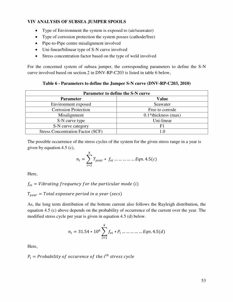
VIV ANALYSIS OF SUBSEA JUMPER SPOOLS
53
Type of Environment the system is exposed to (air/seawater)
Type of corrosion protection the system posses (cathode/free)
Pipe-to-Pipe centre misalignment involved
Uni-linear/bilinear type of S-N curve involved
Stress concentration factor based on the type of weld involved
For the concerned system of subsea jumper, the corresponding parameters to define the S-N
curve involved based on section.2 in DNV-RP-C203 is listed in table 6 below,
Table 6 - Parameters to define the Jumper S-N curve (DNV-RP-C203, 2010)
Parameter to define the S-N curve
Parameter Value
Environment exposed Seawater
Corrosion Protection Free to corrode
Misalignment 0.1*thickness (max)
S-N curve type Uni-linear
S-N curve category F1
Stress Concentration Factor (SCF) 1.0
The possible occurrence of the stress cycles of the system for the given stress range in a year is
given by equation.4.5 (c),
� =∑ ∗ ��= …………… . .
Here,
� = ℎ =
As, the long term distribution of the bottom current also follows the Rayleigh distribution, the
equation 4.5 (c) above depends on the probability of occurrence of the current over the year. The
modified stress cycle per year is given in equation 4.5 (d) below.
� = . ∗ ∑ � ∗�= � …………… . .
Here,
� = ℎ ℎ
VIV ANALYSIS OF SUBSEA JUMPER SPOOLS
54
Based on this S-N curve method, the fatigue life capacity (Tlife) can formally be expressed as in
equation.4.5 (e) below,
� = ∑ � ∗ ��= ∗ ��…………… . .
But, the effect of utilization factor ( ), should be accounted while calculating the actual service life of the system as mentioned in equation.4.3 (a) above.
From this chapter, we have understood the detailed information regarding the steps involved
while performing a VIV analysis, with the help of the industrial available sources. It includes, the
modal analysis of the system using the FEA tool ANSYS, modeling the system environment
based on the extreme sea state condition considered, modeling the system VIV response based
on the DNV-RP-F105 guidelines, selection of the conditions which require detailed fatigue life
assessment and the detailed fatigue life assessment as per DNV-RP-C203 guidelines.
VIV ANALYSIS OF SUBSEA JUMPER SPOOLS
55
CHAPTER 5
ASSUMPTIONS
The analysis performed in the case study involves the following list of assumptions.
The calculated fatigue damage is only with respect to the vortex induced vibration (VIV)
phenomenon. All the other fatigue damage possibilities like, the pipeline thermal
expansion, slugging and flow induced turbulence are not taken into consideration.
Even though, the static analysis is performed to check the jumper configuration integrity,
based on the minimum specified yield strength. All the other conditions like the collapse
and reaction forces on the connector are assumed to be acceptable and within the limits.
The displacement loads on the connector location are neglected. Because, the additional
stress due to this effect can be compensated through the jumper configuration alteration.
The current flow is assumed to be perpendicular and parallel to the jumper configuration
for the out-of-plane and in-plane condition respectively.
Any orientation of the current flow with respect to the jumper profile is neglected.
The mode shapes are assumed to be either pure inline (or) cross-flow oscillations. The
possible combination of these two oscillations based on a percentage is not considered.
Only the tidal and wind induced current are considered to determine the total current
flow on the surface and they are then extrapolated from the free surface to the pipe level.
All the other possibilities of current like the subsurface, near shore and density driven
components of the current flow are neglected.
The tidal velocity at the free surface is assumed to be 1.5 Knots under all the case
studies.
The pipe level is assumed to be 1 meter above the seabed under all the case studies.
The long-term distribution of the current that is considered under all the case studies is
based on some realistic assumptions.
The location parameter (γ) of the long term Weibull distribution is assumed to be zero.
The duration of the storm is assumed as 3 hours in our case study.
Since, the jumpers are assumed as the connectors between the wellhead and the manifold
in our case study. The safety class of the jumper is assumed to be high.
Since, the seabed bathymetry requirement is small, the safety class of the jumper in our
case study is assumed to be well defined type.
The bottom of the pipe is assumed to be at 838mm above the seabed. This shows that the
presence of the trench will not affect the cross-flow VIV.
The added mass effect for the inline type of oscillation is assumed to be equal to the
volume of water displaced by the jumper. Because, the VIV amplitude relative to the
inline oscillations in our case study is minimal.
VIV ANALYSIS OF SUBSEA JUMPER SPOOLS
56
As mentioned in the section 4.5.2 of the DNV-RP-F105, the effect of the added mass
coefficient for a reduced velocity of less than 2.5 can be neglected.
As per the Palmgren-Minor rule, the linear cumulative damage is assumed in our case
study, for the fatigue damage assessment based on the S-N curve.
The Pipe-to-Pipe centre misalignment possible during fabrication of the jumper is
assumed to a maximum value of 0.1 times the thickness or more.
The probability of the current velocity occurrence on a long term basis is assumed in our
case study.
The service fluid inside the jumper system is assumed to be crude oil with a density of
830 kg/m3.
The jumper system pipe material, its size and thickness are assumed to satisfy all its
mechanical design requirements, like the allowable stress, erosion velocity and the
system integrity check respectively.
Based on the assumptions made with respect to the system safety classification, the
fatigue life of the system should be 100 years (or) more, in order to satisfy the design life
of 25 years.
The jumper pipe size is assumed to be 300 NB and uniform throughout the system.
The jumper system is assumed to be without any insulation and all the bends with a
minimum radius of 3 times the outer diameter.
The variation in the probability of the seabed current occurrence is assumed to vary only
based on the tidal current variation at the free surface.
As mentioned in the DNV-RP-F105, the effect of the screening factor on the Eigen
frequency of the system, in order to identify the necessity for the detailed fatigue life
analysis is not neglected.
The possible fatigue damage during the installation of the jumper is not considered in the
total fatigue cycles to failure of the system during service.
This chapter summarizes all the possible limitations that this work would face from a result
accuracy perspective. It also helps us in identifying the possibilities of either improving this
work through addressing the limitations stated (or) extending this background into similar
systems in the future.
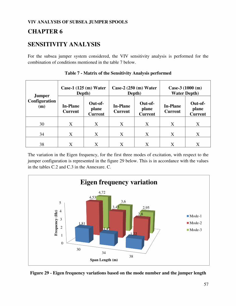
VIV ANALYSIS OF SUBSEA JUMPER SPOOLS
57
CHAPTER 6
SENSITIVITY ANALYSIS
For the subsea jumper system considered, the VIV sensitivity analysis is performed for the
combination of conditions mentioned in the table 7 below.
Table 7 - Matrix of the Sensitivity Analysis performed
Jumper
Configuration
(m)
Case-1 (125 (m) Water
Depth)
Case-2 (250 (m) Water
Depth)
Case-3 (1000 (m)
Water Depth)
In-Plane
Current
Out-of-
plane
Current
In-Plane
Current
Out-of-
plane
Current
In-Plane
Current
Out-of-
plane
Current
30 X X X X X X
34 X X X X X X
38 X X X X X X
The variation in the Eigen frequency, for the first three modes of excitation, with respect to the
jumper configuration is represented in the figure 29 below. This is in accordance with the values
in the tables C.2 and C.3 in the Annexure. C.
Figure 29 - Eigen frequency variations based on the mode number and the jumper length
0
1
2
3
4
5
3034
38
1,81
1,47
1,22
4,53
3,45
2,8
4,72
3,6
2,95
Fre
qu
ency
(H
z)
Span Length (m)
Eigen frequency variation
Mode-1
Mode-2
Mode-3
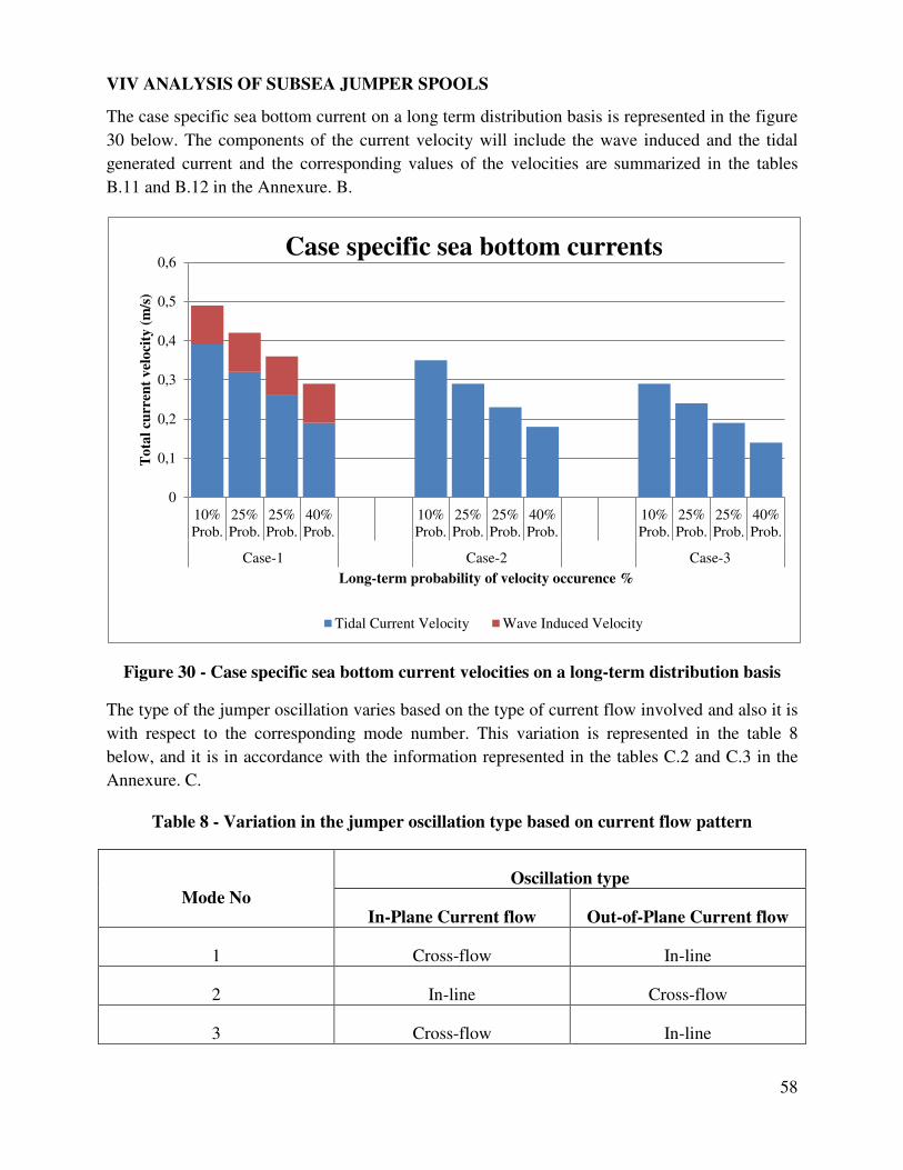
VIV ANALYSIS OF SUBSEA JUMPER SPOOLS
58
The case specific sea bottom current on a long term distribution basis is represented in the figure
30 below. The components of the current velocity will include the wave induced and the tidal
generated current and the corresponding values of the velocities are summarized in the tables
B.11 and B.12 in the Annexure. B.
Figure 30 - Case specific sea bottom current velocities on a long-term distribution basis
The type of the jumper oscillation varies based on the type of current flow involved and also it is
with respect to the corresponding mode number. This variation is represented in the table 8
below, and it is in accordance with the information represented in the tables C.2 and C.3 in the
Annexure. C.
Table 8 - Variation in the jumper oscillation type based on current flow pattern
Mode No Oscillation type
In-Plane Current flow Out-of-Plane Current flow
1 Cross-flow In-line
2 In-line Cross-flow
3 Cross-flow In-line
0
0,1
0,2
0,3
0,4
0,5
0,6
10%
Prob.
25%
Prob.
25%
Prob.
40%
Prob.
10%
Prob.
25%
Prob.
25%
Prob.
40%
Prob.
10%
Prob.
25%
Prob.
25%
Prob.
40%
Prob.
Case-1 Case-2 Case-3
To
tal
curr
ent
vel
oci
ty (
m/s
)
Long-term probability of velocity occurence %
Case specific sea bottom currents
Tidal Current Velocity Wave Induced Velocity
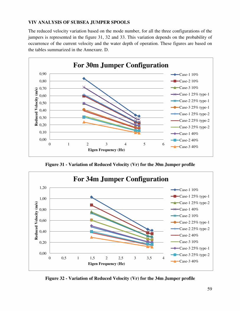
VIV ANALYSIS OF SUBSEA JUMPER SPOOLS
59
The reduced velocity variation based on the mode number, for all the three configurations of the
jumpers is represented in the figure 31, 32 and 33. This variation depends on the probability of
occurrence of the current velocity and the water depth of operation. These figures are based on
the tables summarized in the Annexure. D.
Figure 31 - Variation of Reduced Velocity (Vr) for the 30m Jumper profile
Figure 32 - Variation of Reduced Velocity (Vr) for the 34m Jumper profile
0,00
0,10
0,20
0,30
0,40
0,50
0,60
0,70
0,80
0,90
0 1 2 3 4 5 6
Red
uce
d V
elo
city
(m
/s)
Eigen Frequency (Hz)
For 30m Jumper Configuration
Case-1 10%
Case-2 10%
Case-3 10%
Case-1 25% type-1
Case-2 25% type-1
Case-3 25% type-1
Case-1 25% type-2
Case-2 25% type-2
Case-3 25% type-2
Case-1 40%
Case-2 40%
Case-3 40%
0,00
0,20
0,40
0,60
0,80
1,00
1,20
0 0,5 1 1,5 2 2,5 3 3,5 4
Red
uce
d V
elo
city
(m
/s)
Eigen Frequency (Hz)
For 34m Jumper Configuration
Case-1 10%
Case-1 25% type-1
Case-1 25% type-2
Case-1 40%
Case-2 10%
Case-2 25% type-1
Case-2 25% type-2
Case-2 40%
Case-3 10%
Case-3 25% type-1
Case-3 25% type-2
Case-3 40%
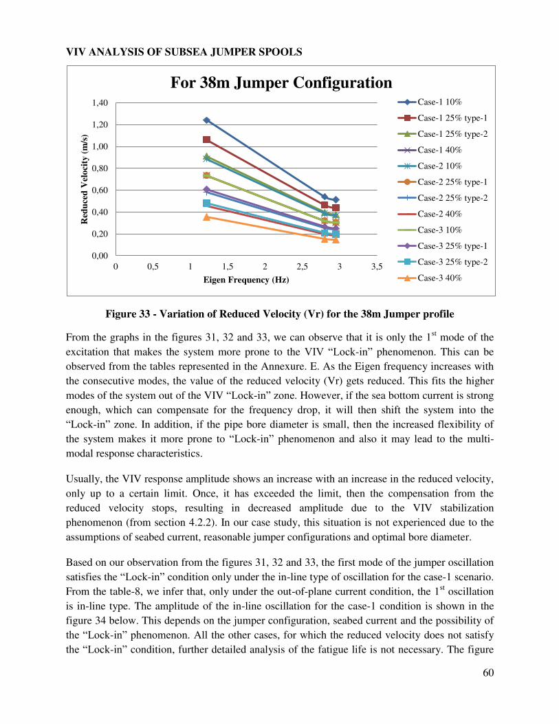
VIV ANALYSIS OF SUBSEA JUMPER SPOOLS
60
Figure 33 - Variation of Reduced Velocity (Vr) for the 38m Jumper profile
From the graphs in the figures 31, 32 and 33, we can observe that it is only the 1st mode of the
excitation that makes the system more prone to the VIV “Lock-in” phenomenon. This can be
observed from the tables represented in the Annexure. E. As the Eigen frequency increases with
the consecutive modes, the value of the reduced velocity (Vr) gets reduced. This fits the higher
modes of the system out of the VIV “Lock-in” zone. However, if the sea bottom current is strong
enough, which can compensate for the frequency drop, it will then shift the system into the
“Lock-in” zone. In addition, if the pipe bore diameter is small, then the increased flexibility of
the system makes it more prone to “Lock-in” phenomenon and also it may lead to the multi-
modal response characteristics.
Usually, the VIV response amplitude shows an increase with an increase in the reduced velocity,
only up to a certain limit. Once, it has exceeded the limit, then the compensation from the
reduced velocity stops, resulting in decreased amplitude due to the VIV stabilization
phenomenon (from section 4.2.2). In our case study, this situation is not experienced due to the
assumptions of seabed current, reasonable jumper configurations and optimal bore diameter.
Based on our observation from the figures 31, 32 and 33, the first mode of the jumper oscillation
satisfies the “Lock-in” condition only under the in-line type of oscillation for the case-1 scenario.
From the table-8, we infer that, only under the out-of-plane current condition, the 1st oscillation
is in-line type. The amplitude of the in-line oscillation for the case-1 condition is shown in the
figure 34 below. This depends on the jumper configuration, seabed current and the possibility of
the “Lock-in” phenomenon. All the other cases, for which the reduced velocity does not satisfy
the “Lock-in” condition, further detailed analysis of the fatigue life is not necessary. The figure
0,00
0,20
0,40
0,60
0,80
1,00
1,20
1,40
0 0,5 1 1,5 2 2,5 3 3,5
Red
uce
d V
elo
city
(m
/s)
Eigen Frequency (Hz)
For 38m Jumper Configuration Case-1 10%
Case-1 25% type-1
Case-1 25% type-2
Case-1 40%
Case-2 10%
Case-2 25% type-1
Case-2 25% type-2
Case-2 40%
Case-3 10%
Case-3 25% type-1
Case-3 25% type-2
Case-3 40%
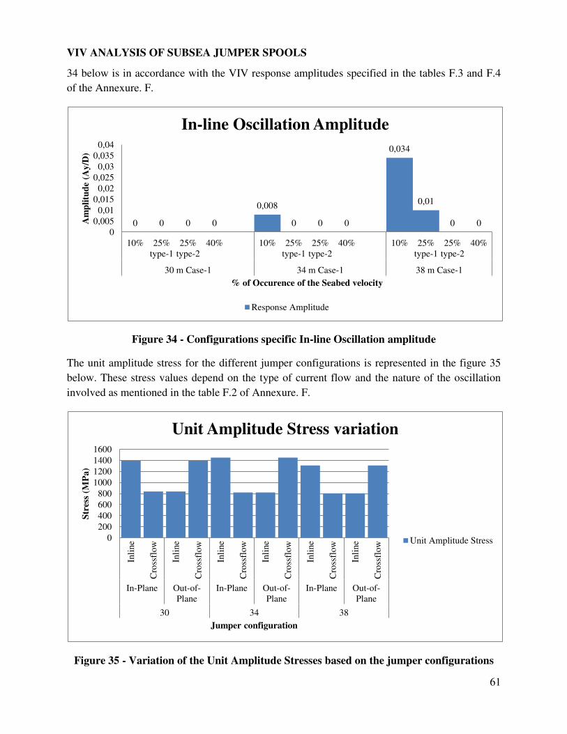
VIV ANALYSIS OF SUBSEA JUMPER SPOOLS
61
34 below is in accordance with the VIV response amplitudes specified in the tables F.3 and F.4
of the Annexure. F.
Figure 34 - Configurations specific In-line Oscillation amplitude
The unit amplitude stress for the different jumper configurations is represented in the figure 35
below. These stress values depend on the type of current flow and the nature of the oscillation
involved as mentioned in the table F.2 of Annexure. F.
Figure 35 - Variation of the Unit Amplitude Stresses based on the jumper configurations
0 0 0 0
0,008
0 0 0
0,034
0,01
0 0 0
0,005
0,01
0,015
0,02
0,025
0,03
0,035
0,04
10% 25%
type-1
25%
type-2
40% 10% 25%
type-1
25%
type-2
40% 10% 25%
type-1
25%
type-2
40%
30 m Case-1 34 m Case-1 38 m Case-1
Am
pli
tud
e (A
y/D
)
% of Occurence of the Seabed velocity
In-line Oscillation Amplitude
Response Amplitude
0
200
400
600
800
1000
1200
1400
1600
Inli
ne
Cro
ssfl
ow
Inli
ne
Cro
ssfl
ow
Inli
ne
Cro
ssfl
ow
Inli
ne
Cro
ssfl
ow
Inli
ne
Cro
ssfl
ow
Inli
ne
Cro
ssfl
ow
In-Plane Out-of-
Plane
In-Plane Out-of-
Plane
In-Plane Out-of-
Plane
30 34 38
Str
ess
(MP
a)
Jumper configuration
Unit Amplitude Stress variation
Unit Amplitude Stress
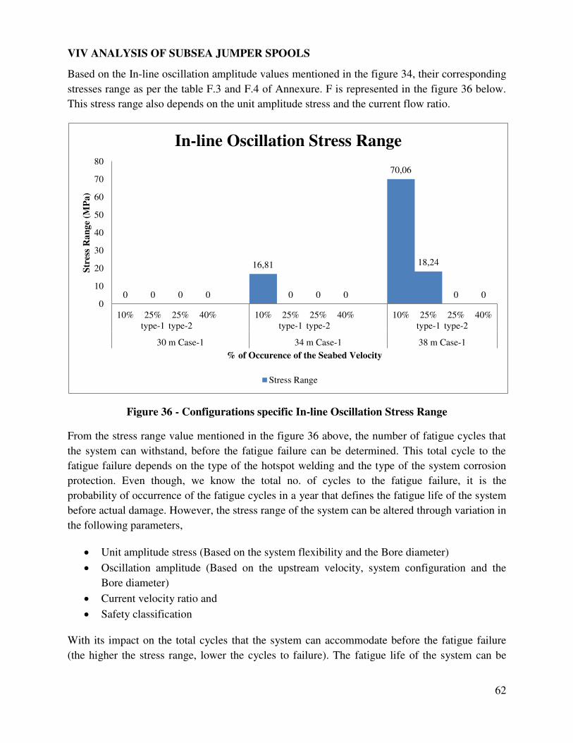
VIV ANALYSIS OF SUBSEA JUMPER SPOOLS
62
Based on the In-line oscillation amplitude values mentioned in the figure 34, their corresponding
stresses range as per the table F.3 and F.4 of Annexure. F is represented in the figure 36 below.
This stress range also depends on the unit amplitude stress and the current flow ratio.
Figure 36 - Configurations specific In-line Oscillation Stress Range
From the stress range value mentioned in the figure 36 above, the number of fatigue cycles that
the system can withstand, before the fatigue failure can be determined. This total cycle to the
fatigue failure depends on the type of the hotspot welding and the type of the system corrosion
protection. Even though, we know the total no. of cycles to the fatigue failure, it is the
probability of occurrence of the fatigue cycles in a year that defines the fatigue life of the system
before actual damage. However, the stress range of the system can be altered through variation in
the following parameters,
Unit amplitude stress (Based on the system flexibility and the Bore diameter)
Oscillation amplitude (Based on the upstream velocity, system configuration and the
Bore diameter)
Current velocity ratio and
Safety classification
With its impact on the total cycles that the system can accommodate before the fatigue failure
(the higher the stress range, lower the cycles to failure). The fatigue life of the system can be
0 0 0 0
16,81
0 0 0
70,06
18,24
0 0 0
10
20
30
40
50
60
70
80
10% 25%
type-1
25%
type-2
40% 10% 25%
type-1
25%
type-2
40% 10% 25%
type-1
25%
type-2
40%
30 m Case-1 34 m Case-1 38 m Case-1
Str
ess
Ra
ng
e (M
Pa
)
% of Occurence of the Seabed Velocity
In-line Oscillation Stress Range
Stress Range
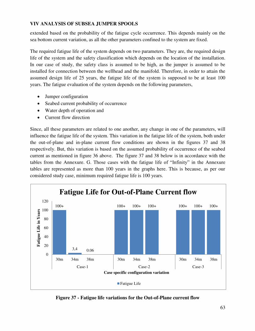
VIV ANALYSIS OF SUBSEA JUMPER SPOOLS
63
extended based on the probability of the fatigue cycle occurrence. This depends mainly on the
sea bottom current variation, as all the other parameters confined to the system are fixed.
The required fatigue life of the system depends on two parameters. They are, the required design
life of the system and the safety classification which depends on the location of the installation.
In our case of study, the safety class is assumed to be high, as the jumper is assumed to be
installed for connection between the wellhead and the manifold. Therefore, in order to attain the
assumed design life of 25 years, the fatigue life of the system is supposed to be at least 100
years. The fatigue evaluation of the system depends on the following parameters,
Jumper configuration
Seabed current probability of occurrence
Water depth of operation and
Current flow direction
Since, all these parameters are related to one another, any change in one of the parameters, will
influence the fatigue life of the system. This variation in the fatigue life of the system, both under
the out-of-plane and in-plane current flow conditions are shown in the figures 37 and 38
respectively. But, this variation is based on the assumed probability of occurrence of the seabed
current as mentioned in figure 36 above. The figure 37 and 38 below is in accordance with the
tables from the Annexure. G. Those cases with the fatigue life of “Infinity” in the Annexure
tables are represented as more than 100 years in the graphs here. This is because, as per our
considered study case, minimum required fatigue life is 100 years.
Figure 37 - Fatigue life variations for the Out-of-Plane current flow
100+
3,4 0.06
100+ 100+ 100+ 100+ 100+ 100+
0
20
40
60
80
100
120
30m 34m 38m 30m 34m 38m 30m 34m 38m
Case-1 Case-2 Case-3
Fa
tig
ue
Lif
e in
Yea
rs
Case specific configuration variation
Fatigue Life for Out-of-Plane Current flow
Fatigue Life
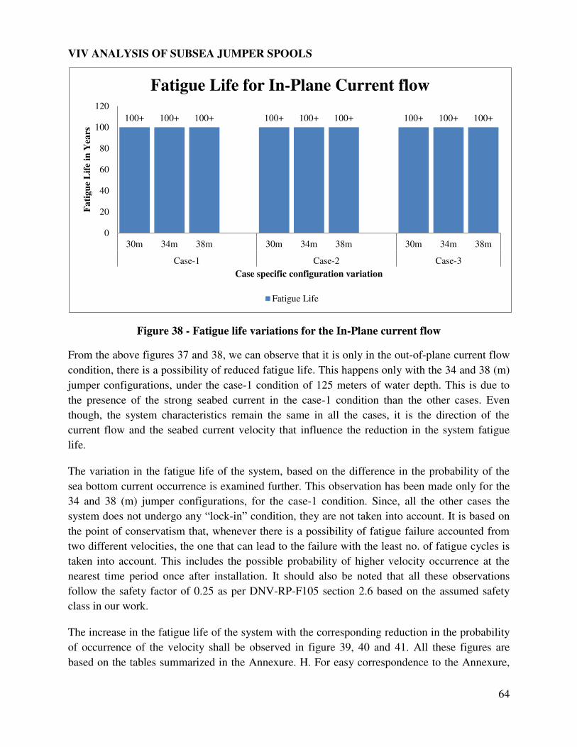
VIV ANALYSIS OF SUBSEA JUMPER SPOOLS
64
Figure 38 - Fatigue life variations for the In-Plane current flow
From the above figures 37 and 38, we can observe that it is only in the out-of-plane current flow
condition, there is a possibility of reduced fatigue life. This happens only with the 34 and 38 (m)
jumper configurations, under the case-1 condition of 125 meters of water depth. This is due to
the presence of the strong seabed current in the case-1 condition than the other cases. Even
though, the system characteristics remain the same in all the cases, it is the direction of the
current flow and the seabed current velocity that influence the reduction in the system fatigue
life.
The variation in the fatigue life of the system, based on the difference in the probability of the
sea bottom current occurrence is examined further. This observation has been made only for the
34 and 38 (m) jumper configurations, for the case-1 condition. Since, all the other cases the
system does not undergo any “lock-in” condition, they are not taken into account. It is based on
the point of conservatism that, whenever there is a possibility of fatigue failure accounted from
two different velocities, the one that can lead to the failure with the least no. of fatigue cycles is
taken into account. This includes the possible probability of higher velocity occurrence at the
nearest time period once after installation. It should also be noted that all these observations
follow the safety factor of 0.25 as per DNV-RP-F105 section 2.6 based on the assumed safety
class in our work.
The increase in the fatigue life of the system with the corresponding reduction in the probability
of occurrence of the velocity shall be observed in figure 39, 40 and 41. All these figures are
based on the tables summarized in the Annexure. H. For easy correspondence to the Annexure,
100+ 100+ 100+ 100+ 100+ 100+ 100+ 100+ 100+
0
20
40
60
80
100
120
30m 34m 38m 30m 34m 38m 30m 34m 38m
Case-1 Case-2 Case-3
Fa
tig
ue
Lif
e in
Yea
rs
Case specific configuration variation
Fatigue Life for In-Plane Current flow
Fatigue Life
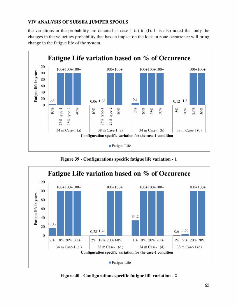
VIV ANALYSIS OF SUBSEA JUMPER SPOOLS
65
the variations in the probability are denoted as case-1 (a) to (f). It is also noted that only the
changes in the velocities probability that has an impact on the lock-in zone occurrence will bring
change in the fatigue life of the system.
Figure 39 - Configurations specific fatigue life variation - 1
Figure 40 - Configurations specific fatigue life variation - 2
3,4
100+ 100+ 100+
0,06 1,28
100+ 100+
6,8
100+ 100+ 100+
0,12 1,6
100+ 100+
0
20
40
60
80
100
120
10%
25%
typ
e-1
25%
typ
e-2
40%
10%
25%
typ
e-1
25%
typ
e-2
40%
5%
20%
25%
50%
5%
20%
25%
50%
34 m Case-1 (a) 38 m Case-1 (a) 34 m Case-1 (b) 38 m Case-1 (b)
Fa
tig
ue
life
in
yea
rs
Configuration specific variation for the case-1 condition
Fatigue Life variation based on % of Occurence
Fatigue Life
17,12
100+ 100+ 100+
0,28 1,76
100+ 100+
34,2
100+ 100+ 100+
0,6 3,56
100+ 100+
0
20
40
60
80
100
120
2% 18% 20% 60% 2% 18% 20% 60% 1% 9% 20% 70% 1% 9% 20% 70%
34 m Case-1 (c ) 38 m Case-1 (c ) 34 m Case-1 (d) 38 m Case-1 (d)
Fa
tig
ue
life
in
yea
rs
Configuration specific variation for the case-1 condition
Fatigue Life variation based on % of Occurence
Fatigue Life
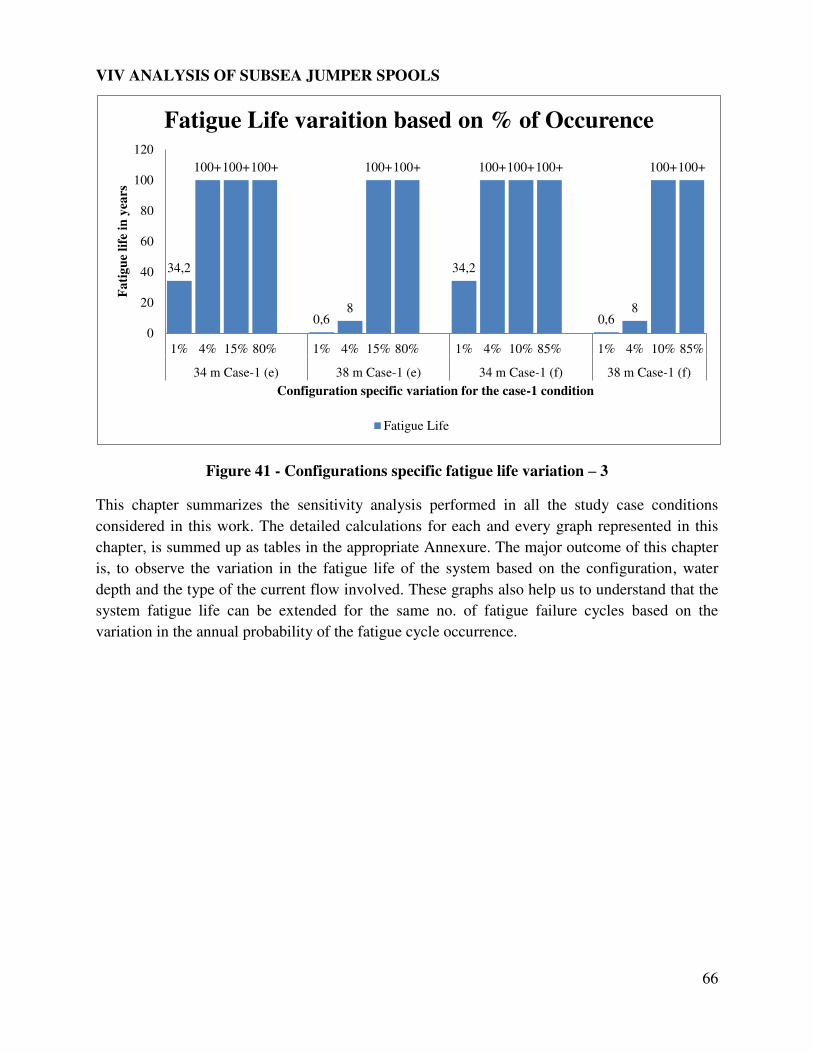
VIV ANALYSIS OF SUBSEA JUMPER SPOOLS
66
Figure 41 - Configurations specific fatigue life variation – 3
This chapter summarizes the sensitivity analysis performed in all the study case conditions
considered in this work. The detailed calculations for each and every graph represented in this
chapter, is summed up as tables in the appropriate Annexure. The major outcome of this chapter
is, to observe the variation in the fatigue life of the system based on the configuration, water
depth and the type of the current flow involved. These graphs also help us to understand that the
system fatigue life can be extended for the same no. of fatigue failure cycles based on the
variation in the annual probability of the fatigue cycle occurrence.
34,2
100+ 100+ 100+
0,6 8
100+ 100+
34,2
100+ 100+ 100+
0,6 8
100+ 100+
0
20
40
60
80
100
120
1% 4% 15% 80% 1% 4% 15% 80% 1% 4% 10% 85% 1% 4% 10% 85%
34 m Case-1 (e) 38 m Case-1 (e) 34 m Case-1 (f) 38 m Case-1 (f)
Fa
tig
ue
life
in
yea
rs
Configuration specific variation for the case-1 condition
Fatigue Life varaition based on % of Occurence
Fatigue Life
VIV ANALYSIS OF SUBSEA JUMPER SPOOLS
67
CHAPTER 7
DISCUSSION
Based on the sensitivity analysis performed, for the considered M-shaped profile of the rigid
jumper, for three different configurations like the 30/34/38 meters of length, the following
observations are discussed. The three different configurations, considered in our study, are based
on the possible requirements from the assumed subsea layout as mentioned in Annexure. A. The
analysis results depend on the seabed depth of operation of the jumper like the 125/250/1000
meters of water depth and the direction of the current flow, which can be either in-plane or out-
of-plane.
7.1 Under In-Plane Current Condition
In the sensitivity analysis, whenever the considered jumper system is exposed to the assumed in-
plane current flow, it will satisfy the condition of the demanded fatigue life. The demanded
fatigue life in our case of study is 100 years or more, in order to meet the design life of 25 years.
This result remains the same, irrespective of the jumper profile and the water depth of operation
the system involves.
This is because under in-plane current flow the first mode of excitation of the system is the
cross-flow type of oscillation. Since, the effective area of the jumper involved in the VIV is
much less in comparison to that of the out-of-plane current condition, as mentioned in the
figures.16 and 17, the possibility of the system to fall in the lock-in bandwidth is lesser. This
reduces the chance of the system to experience the larger stress due to large amplitude of
oscillation.
However, if the vertical doglegs of the system like V1, V3 and V5 as mentioned in the
Annexure. A gets increased, then the Eigen frequency of the system gets reduced, this is due to
the increased effective mass and length of the system. This reduction in the Eigen frequency can
enhance the possibility of the lock-in to happen even under the in-plane current flow condition.
The same result of increased lock-in possibility can be attained, if the current to which the
system is exposed near the seabed is increased than the considered value as in our case study.
All the above discussed conditions that have its impact on the VIV occurrence are pertained only
to our considered pipe size of 300 NB. Once the pipe size differs, the system flexibility
requirement will change resulting in a different configuration than the one considered in our case
study. This difference in the configuration, will impact on the Eigen frequency of the system
through effective mass and length of the system variables involved. It also varies the fluid-
surface contact area, which has its influence on the VIV generation strength. Hence, it can result
VIV ANALYSIS OF SUBSEA JUMPER SPOOLS
68
in a different limiting criterion for the VIV possibility, based on the jumper configuration from
that of our 300 NB pipe size study case.
However, in our case study with the extreme environmental and system detail assumptions
involved, the condition of the system design life of 25 years is satisfied. This can only be
attained if the system fatigue life is 100 years (or) more as in our case. Under in-plane current
condition, for all the three configurations, under all the three possible water depths of operation,
the design life is met, because of the absence of the VIV lock-in phenomenon.
7.2 Under Out-of-Plane Current Condition
Since, the first mode of excitation under the out-of-plane current condition is the inline type of
oscillation, the possibility for the jumper system to experience the lock-in phenomenon is much
higher than in the in-plane current condition. This possibility would increase further with the
increase in the unsupported length of the jumper configuration involved. But, based on the water
depth of application, the critical length of the configuration that does not suffer any damage from
the VIV phenomenon will change.
Based on our sensitive analysis study, we can observe that all the three possible configurations of
the jumpers will satisfy the condition of 100 years (or) more fatigue life, under the 250 and 1000
meters of water depth scenario. But, this is not the case for 125 meters of water depth condition.
The minimum decay of water particle velocity from the surface, results in a much higher seabed
current velocity in the 125 meter condition, in comparison to the 250 and 1000 meters of water
depth scenario.
This presence of the higher seabed current in the 125 meters of water depth scenario has resulted
in a restricted critical jumper length of 30 meters, from the application perspective. The low
frequency characteristics of the jumper based on the higher unsupported length have made the 34
and 38 meter jumper configuration more prone to the VIV phenomenon under this water depth
condition.
Again, as mentioned in the section 7.1, the sensitivity analysis results are subjective to the
considered assembly details of the jumper, with a pipe size of 300 NB and exposed to the
assumed extreme environmental conditions. With any changes in these assumptions, the severity
of the VIV phenomenon that the system is exposed to would differ.
Even, if the jumper configuration is exposed to the VIV phenomenon, it is the probability of
occurrence of the VIV influencing current per year that defines the system survival time. This
variation in the fatigue life based on the probability of occurrence per year can be observed in
our case study plots. This variation in the fatigue life depends only on the velocity that influences
VIV on the system. Since, in our case study the jumpers considered are assumed to be a
connector between the wellhead and the manifold, the usage factor corresponding to a higher
VIV ANALYSIS OF SUBSEA JUMPER SPOOLS
69
class of safety is used. This demands a fatigue life of 100 years or more in order to satisfy the
designed service life of 25 years.
Whenever, there are two different velocities that cause two different fatigue stresses in the
system, then the fatigue life of the system is calculated based on the least possible fatigue life out
of the two stresses. This involves the relationship between the S-N curve and the probability of
occurrence per year. Since, the probability of the velocity occurrence will be different every
year, a long term Rayleigh distribution of seabed velocity is usually considered to define the
service life of the system.
Since, the 34 and 38 meters of jumper configuration experience the VIV effect, for the 125
meters of water depth scenario they do not satisfy the 100 years (or) more fatigue life
requirement. This makes it clear that the 30 meter jumper configuration is the critical jumper
length of the 125 meter water depth condition. However, as the jumper length is based on the
seabed layout any length requirement of the jumper beyond 30 meters for the 125 meters water
depth condition will require VIV mitigation measures to be considered. On the other hand, for
the 250 and 1000 meters of water depth scenario, all the three configurations of jumpers can be
successfully used, as they do meet the service life of the system.
7.3 Uncertainty
Even though, this sensitivity analysis aims to study the jumper fatigue life variation based on the
difference in their configuration, water depth of operation and current flow conditions. The
accuracy of our study results faces some uncertainty based on our assumptions listed in chapter
5. With the usage of real time site specific data, the accuracy of our realistic outcome can be
improvised. But still the system fatigue life evaluation always remains case specific.
It should also be noted that, this fatigue life assessment focuses only on the fatigue damage from
the VIV phenomenon, it does not include the fatigue damages from all other possibilities like,
pipeline thermal expansion, slugging and flow induced turbulence. So, this result refers to the
system total fatigue life, only if all other possibilities of fatigue damage are rectified. Any type of
change that has its impact on the jumper characteristics like the fluid involved in the
transportation, shape of the jumper, diameter of the pipe involved etc., will result in a different
case specific critical length requirement. Moreover, any possibility of fatigue during the
installation phase of the jumper will result in a corresponding reduction in the total fatigue cycles
to failure during the service of the system.
Any type of update, on the standards used in our case study, may also account for the uncertainty
associated with our study results. All the calculations had been performed based on the referred
year of release of the standards.
VIV ANALYSIS OF SUBSEA JUMPER SPOOLS
70
CHAPTER 8
CONCLUSION AND RECOMMENDATION
The conclusion of this thesis work is divided into the following sections,
The subsea rigid jumpers, which are short rigid steel pipe sections that provide the interface
between the subsea structures such as pipelines to manifolds, trees to flowlines and pipelines to
risers, are not static elements as considered by many designers. In addition to satisfying the
mechanical strength requirements like the pipeline thermal expansion, pipeline installation
inaccuracies and lower reaction forces on the connection terminals, these jumpers should also
satisfy the fatigue life requirements, in order to avoid any fatigue failure throughout the design
life. The presence of the complex shape to meet its mechanical design requirements with larger
unsupported lengths, results in the reduced Eigen frequency of the system making it more prone
to VIV fatigue damage. The critical length of the jumper that defines the requirement for the
VIV mitigation measure will change based on several factors like the jumper shape, jumper
characteristics, seabed current, location of installation and the angle of the current flow.
For any typical jumper profile (like the Inverted-U, M (or) Z-shape), the fatigue failure cycles
varies based on the direction of the current flow, seabed current condition, location of service
and the Eigen frequency characteristics of the system. The influence of the direction of current
flow upon the fatigue cycles of the system is based on the effective area of the jumper that is
involved in the VIV phenomenon and also the possible type oscillation for the 1st excitation
mode. Even though, there are possibilities for the multi-modal response, the 1st excitation mode
is treated to be crucial in most of the cases due to the low Eigen frequency of the system and the
lower seabed current velocity dependence. In case of the in-plane current condition, the 1st mode
of excitation is the cross-flow type with a lock-in velocity bandwidth of 2-16 m/s, whereas for
the out-of-plane current condition it is the in-line type of oscillation with a lock-in velocity
bandwidth of 0.91-4.3 m/s. This explains that the probability of the same system with the same
current velocity condition to fall in the lock-in zone is much higher for the out-of-plane current
flow than the in-plane current. However, this can be compensated based on the variation in the
effective area that is involved in the vortex generation.
The phenomenon of multi-modal response can be possible for those systems with either much
lower Eigen frequency characteristics (or) much stronger seabed current exposure. The presence
of the stronger seabed current will influence the strength of the generated vortices. For the
scenario with a stronger seabed current, the critical length (the maximum unsupported length
without the possibility of VIV) of the jumper is reduced. Once we proceed from shallow water
zone towards deep water depths, the possibility of strong seabed current is greatly reduced this is
due to the exponential decay of the water particle velocity from the surface to the seabed. This
VIV ANALYSIS OF SUBSEA JUMPER SPOOLS
71
means that those systems that require VIV mitigation measure in the shallow water depth does
not require any VIV mitigation measure in deeper water conditions.
For the same jumper system with the same direction of current flow and with the same seabed
current velocity, the fatigue life requirement would differ based on the location of its installation.
This is due to the difference in the safety factor which depends on the location uncertainty.
Those systems that are close to the wellhead involve higher safety factor than those that are
installed close to the platform.
Even though, all the above mentioned characteristics are related to one another in determining
the total no. of fatigue cycles of the system for a considered case of study, it is the probability of
occurrence of the stress range from one year that defines the fatigue life of the system. This
means that, even if the no. of fatigue cycles to failure is less for a particular stress range, this will
not be the fatigue life determining criterion of the system, if the probability of occurrence of that
particular stress is the rarest. But, this influence of the probability of occurrence on the fatigue
life of the system is only possible for those conditions that satisfy the lock-in criterion.
This work was carried out to address the present lack in the industry in order to perform the VIV
analysis for the complex shaped jumper spools. But, the guidelines were used from the existing
standard for pipelines DNV-RP-F105, since there is no specific standard been available in the
industry for the subsea spools. Due to insufficient data on the methodology for carrying out this
VIV analysis for the jumper spools, this work has confined its scope to only a typical M-shaped
jumper profile with much of its time been spent on understanding the VIV phenomenon and the
methodology it requires to perform the task involving some alteration from the existing
guidelines for the pipeline. The methodology in this work primarily focuses on the possibility of
the system to fall in the lock-in zone under respective excitation modes. This is because the
amplitude of oscillation and its resulting stresses from the resonance condition are huge in
comparison to other conditions. This will have a huge impact on the fatigue life of the system
than in any other case. With the understanding of the VIV phenomenon and the methodology
guideline from this work as the background skeleton, this work can be improved or extended
further in the following paths.
Rectifying the assumptions would improve the results accuracy of this work.
Addition of the torsion component of stress induced in the vertical legs of the jumpers to
the stress range wherever possible would result in a realistic study. This depends on the
comparison of the torsion stress value to the bending stress before adding.
The same methodology of this work can be extended further to all other possible shapes
of the jumper spools to determine the ideal jumper profile that does not require any VIV
mitigations even under the severe environmental case.
Through comparison of the different jumper profile results, any extension of the existing
standard DNV-RP-F105 to make it applicable also for the jumper spools can be done.
VIV ANALYSIS OF SUBSEA JUMPER SPOOLS
72
CHAPTER 9
REFERENCE
Abeele, F. V., Voorde, J. V., and Goes, P. (2008). Numerical Modelling of Vortex Induced
Vibrations in Submarine Pipelines. COMSOL Conference. Hannover.
Achenbach, E., and Heinecke, E. (1981). On vortex shedding from smooth and rough
cylinders in the range of Reynolds numbers 6x10³ to 5x10
6. Journal of fluid mechanics, 109,
239-251.
Bai, Y., and Bai, Q. (2005). Subsea Pipelines and Risers. Kidlington: Elsevier.
Bai, Y., and Bai, Q. (2012). Subsea Engineering Handbook. Burlington: Gulf Professional
Publishing.
Bishop, R. E. D. and Hassan, A. Y. (1964). The lift and drag forces on a circular cylinder
oscillating in a flowing fluid. Proceeding of the Royal Society of London, Series A 277, 51-
75.
Blevins, R. D. (2001). Flow Induced Vibrations. Florida: Krieger Publishing Company.
Carruth, A. L., and Cerkovnik, M. E. (2007). Jumper VIV – New Issues for New Frontiers.
17th
International Offshore and Polar Engineering Conference. Houston, Texas.
Coder, D. W. (1982). The Strouhal Number of Vortex Shedding from Marine Risers in
Currents at Super-Critical Reynolds Number. 14th
Annual Offshore Technology Conference.
Paper 4318.
DNV-OS-J101. (2014). Det Norske Veritas Offshore Standards, Design of Offshore Wind
Turbine Structures. Oslo, Norway.
DNV-RP-C203. (2010). Det Norske Veritas Recommended Practice, Fatigue Design of
Offshore Steel Structures. Oslo, Norway.
DNV-RP-F105. (2006). Det Norske Veritas Recommended Practice, Free Spanning
Pipelines. Oslo, Norway.
Griffin, O.H., and Ramberg, S. E. (1974). The Vortex Street Wakes of Vibrating Cylinders.
Journal of Fluid Mechanics, 66, 553-576.
Gudmestad, O. T. (2015). Marine Technology and Operations (Theory and Practice).
Southampton: WIT Press.

VIV ANALYSIS OF SUBSEA JUMPER SPOOLS
73
Guo, B., Song, S., Chacko, J., and Ghalambor, A. (2005). Offshore Pipelines. Burlington:
Gulf Professional Publishing.
Jauvtis, N., and Williamson, C. (2003). Vortex Induced Vibration of a Cylinder with Two
Degrees of Freedom. Journal of Fluids and Structures, 17, pp. 1035-1042.
Kenny, J. P. (1993). Structural analysis of pipeline spans. Offshore Technology Information.
HMSO.
Keulegan, G. H. and Carpenter, L. H. (1958). Forces on cylinders and plates in an oscillating
fluid. Journal of Research of the National Bureau Standards, 60, No. 5, 423-440.
Koopman, G. H. (1967). The Vortex Wakes of Vibrating Cylinders at low Reynolds
Numbers. Journal of Fluid Mechanics, 28, 501-512.
Lienhard, I. H. (1966). Synopsis of lift, drag and vortex frequency data for rigid circular
cylinders. Washington: Washington State University.
Massey, B. S. (1979). Mechanics of Fluids. New York: Van Nostrand Reinhold.
Newman, J. N. (1977). Marine Hydrodynamics. Massachusetts: The Massachusetts Institute
of Technology.
Ongoren, A., and Rockwell, D. (1988). Flow Structure from on Oscillatory Cylinder. Journal
of Fluid Mechanics, 191, 197-245.
Palmer, A. C., and King, R. A. (2004). Subsea Pipeline Engineering. Oklahoma: PennWell
Corporation.
Perry, A. E., Chong, M. S., and Lim, T. T. (1982). The vortex shedding process behind two
dimensional bluff bodies. Journal of fluid mechanics, 116, 77-90.
Prandtl, L. (1904). Uber Flussigkeitsbewegungen bei sehr kleiner reibung. Verhandlg. III.
Intern. Math. Kongr. Heidelberg, 484-491.
Roshko, A. (1954). On the Drag and Vortex Shedding Frequency of Two Dimensional Bluff
Bodies. National Advisory Committee for Aeronautics Report.
Sarpkaya, T. (1978). Fluid forces on oscillating cylinders. Journal of Waterway, Port, Costal
and Ocean Division, 104(WW4), 275-290.
Schlichting, H. (1968). Boundary Layer Theory. New York: McGraw- Hill Book Company.

VIV ANALYSIS OF SUBSEA JUMPER SPOOLS
74
Skop, R. A., Griffin, O. M., and Ramberg, S. E. (1977). Strumming Predictions for the
SEACON II Experimental Mooring. Offshore Technology Conference. Paper OTC 2491,
May 1977.
Stansby, P. K. (1976). The Locking on of Vortex Shedding due to the Cross Stream
Vibration of Circular Cylinder in Uniform and Shear Flow. Journal of Fluid Mechanics, 74,
641-665.
Strouhal, V. (1878). Ueber eine besondere Art der Tonerregung. In: Annalen der Physik und
Chemie. Leipzig, NF. Bd. V, H. 10, S. 216-251.
Tanida, Y., Okajima, A., and Watanabe, Y. (1973). Stability of a Circular Cylinder
Oscillating in Uniform Flow or Wake. Journal of Fluid Mechanics, 61, 769-784.
Torum, A., and Anand, N. M. (1985). Free Span Vibrations of Submarine Pipelines in Steady
flows – Effect of Free Stream Turbulence on Mean Drag Coefficient. Journal of Energy
Resource Technology, 107, 415-420.
Vandiver, J. K. (1983). Drag Coefficients of Long Flexible Cylinders. Offshore Technology
Conference, Paper OTC 4490, May 1977.
Williamson, C. H. K. and Roshka, A. (1988). Vortex formation in the wake of an oscillating
cylinder. Journal of Fluid and Structures, 2, 355-381.
Wootton, L. R. (1991). Vortex-Induced Forces. Dynamics of Marine Substructure, London.
Zdravkovich, M. M. (1982). Review and classification of various aerodynamic and hydrodynamic means for suppressing vortex shedding. Journal of Wind Engineering and
Industrial Aerodynamics, 7, 145-189.

VIV ANALYSIS OF SUBSEA JUMPER SPOOLS
75
ANNEXURES
ANNEXURE – A
JUMPER MODELLING
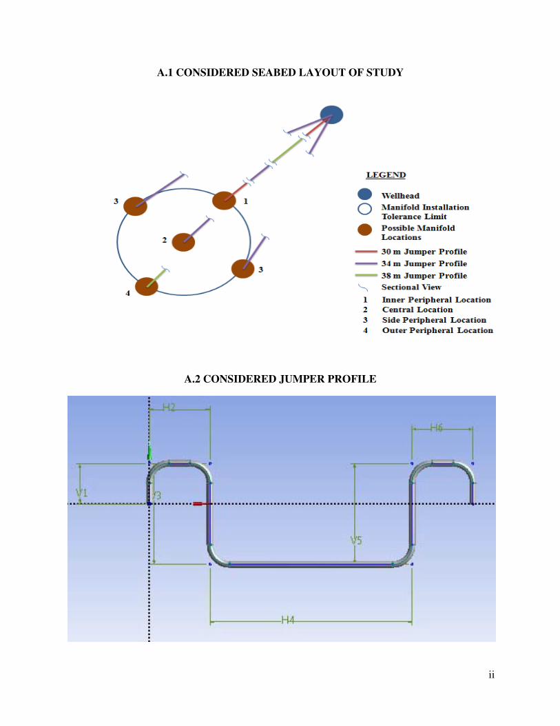
ii
A.1 CONSIDERED SEABED LAYOUT OF STUDY
A.2 CONSIDERED JUMPER PROFILE
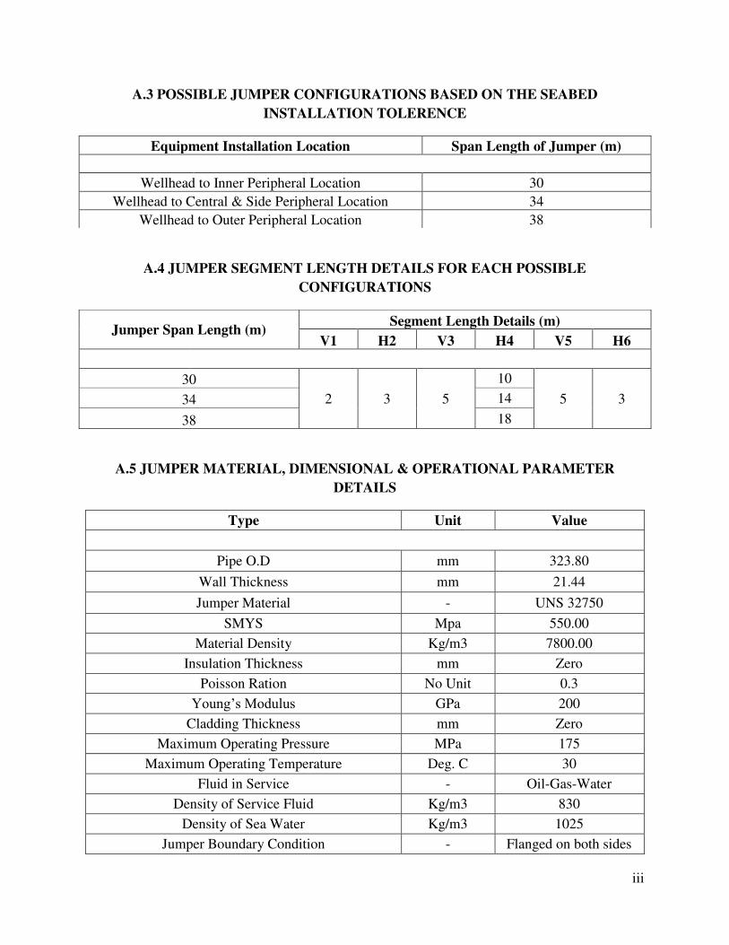
iii
A.3 POSSIBLE JUMPER CONFIGURATIONS BASED ON THE SEABED
INSTALLATION TOLERENCE
A.4 JUMPER SEGMENT LENGTH DETAILS FOR EACH POSSIBLE
CONFIGURATIONS
A.5 JUMPER MATERIAL, DIMENSIONAL & OPERATIONAL PARAMETER
DETAILS
Type Unit Value
Pipe O.D mm 323.80
Wall Thickness mm 21.44
Jumper Material - UNS 32750
SMYS Mpa 550.00
Material Density Kg/m3 7800.00
Insulation Thickness mm Zero
Poisson Ration No Unit 0.3
Young’s Modulus GPa 200
Cladding Thickness mm Zero
Maximum Operating Pressure MPa 175
Maximum Operating Temperature Deg. C 30
Fluid in Service - Oil-Gas-Water
Density of Service Fluid Kg/m3 830
Density of Sea Water Kg/m3 1025
Jumper Boundary Condition - Flanged on both sides
Equipment Installation Location Span Length of Jumper (m)
Wellhead to Inner Peripheral Location 30
Wellhead to Central & Side Peripheral Location 34
Wellhead to Outer Peripheral Location 38
Jumper Span Length (m) Segment Length Details (m)
V1 H2 V3 H4 V5 H6
30
2 3 5
10
5 3 34 14
38 18

ANNEXURE – B
ENVIRONMENT MODELLING
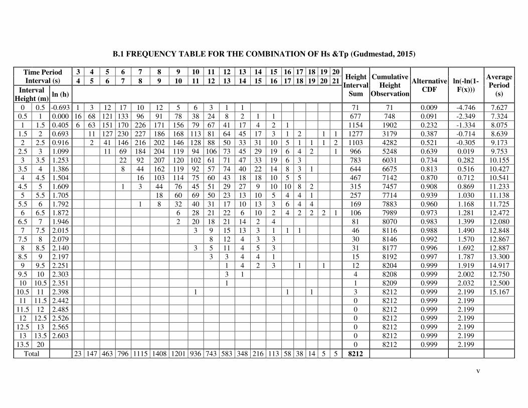
v
B.1 FREQUENCY TABLE FOR THE COMBINATION OF Hs &Tp (Gudmestad, 2015)
Time Period
Interval (s)
3 4 5 6 7 8 9 10 11 12 13 14 15 16 17 18 19 20 Height
Interval
Sum
Cumulative
Height
Observation
Alternative
CDF
ln(-ln(1-
F(x)))
Average
Period
(s)
4 5 6 7 8 9 10 11 12 13 14 15 16 17 18 19 20 21
Interval
Height (m) ln (h)
0 0.5 -0.693 1 3 12 17 10 12 5 6 3 1 1 71 71 0.009 -4.746 7.627
0.5 1 0.000 16 68 121 133 96 91 78 38 24 8 2 1 1 677 748 0.091 -2.349 7.324
1 1.5 0.405 6 63 151 170 226 171 156 79 67 41 17 4 2 1 1154 1902 0.232 -1.334 8.075
1.5 2 0.693 11 127 230 227 186 168 113 81 64 45 17 3 1 2 1 1 1277 3179 0.387 -0.714 8.639
2 2.5 0.916 2 41 146 216 202 146 128 88 50 33 31 10 5 1 1 1 2 1103 4282 0.521 -0.305 9.173
2.5 3 1.099 11 69 184 204 119 94 106 73 45 29 19 6 4 2 1 966 5248 0.639 0.019 9.753
3 3.5 1.253 22 92 207 120 102 61 71 47 33 19 6 3 783 6031 0.734 0.282 10.155
3.5 4 1.386 8 44 162 119 92 57 74 40 22 14 8 3 1 644 6675 0.813 0.516 10.427
4 4.5 1.504 16 103 114 75 60 43 18 18 10 5 5 467 7142 0.870 0.712 10.541
4.5 5 1.609 1 3 44 76 45 51 29 27 9 10 10 8 2 315 7457 0.908 0.869 11.233
5 5.5 1.705 18 60 69 50 23 13 10 5 4 4 1 257 7714 0.939 1.030 11.138
5.5 6 1.792 1 8 32 40 31 17 10 13 3 6 4 4 169 7883 0.960 1.168 11.725
6 6.5 1.872 6 28 21 22 6 10 2 4 2 2 2 1 106 7989 0.973 1.281 12.472
6.5 7 1.946 2 20 18 21 14 2 4 81 8070 0.983 1.399 12.080
7 7.5 2.015 3 9 15 13 3 1 1 1 46 8116 0.988 1.490 12.848
7.5 8 2.079 8 12 4 3 3 30 8146 0.992 1.570 12.867
8 8.5 2.140 3 5 11 4 5 3 31 8177 0.996 1.692 12.887
8.5 9 2.197 3 3 4 4 1 15 8192 0.997 1.787 13.300
9 9.5 2.251 1 4 2 3 1 1 12 8204 0.999 1.919 14.917
9.5 10 2.303 3 1 4 8208 0.999 2.002 12.750
10 10.5 2.351 1 1 8209 0.999 2.032 12.500
10.5 11 2.398 1 1 1 3 8212 0.999 2.199 15.167
11 11.5 2.442 0 8212 0.999 2.199
11.5 12 2.485 0 8212 0.999 2.199
12 12.5 2.526 0 8212 0.999 2.199
12.5 13 2.565 0 8212 0.999 2.199
13 13.5 2.603 0 8212 0.999 2.199
13.5 20 0 8212 0.999 2.199
Total 23 147 463 796 1115 1408 1201 936 743 583 348 216 113 58 38 14 5 5 8212
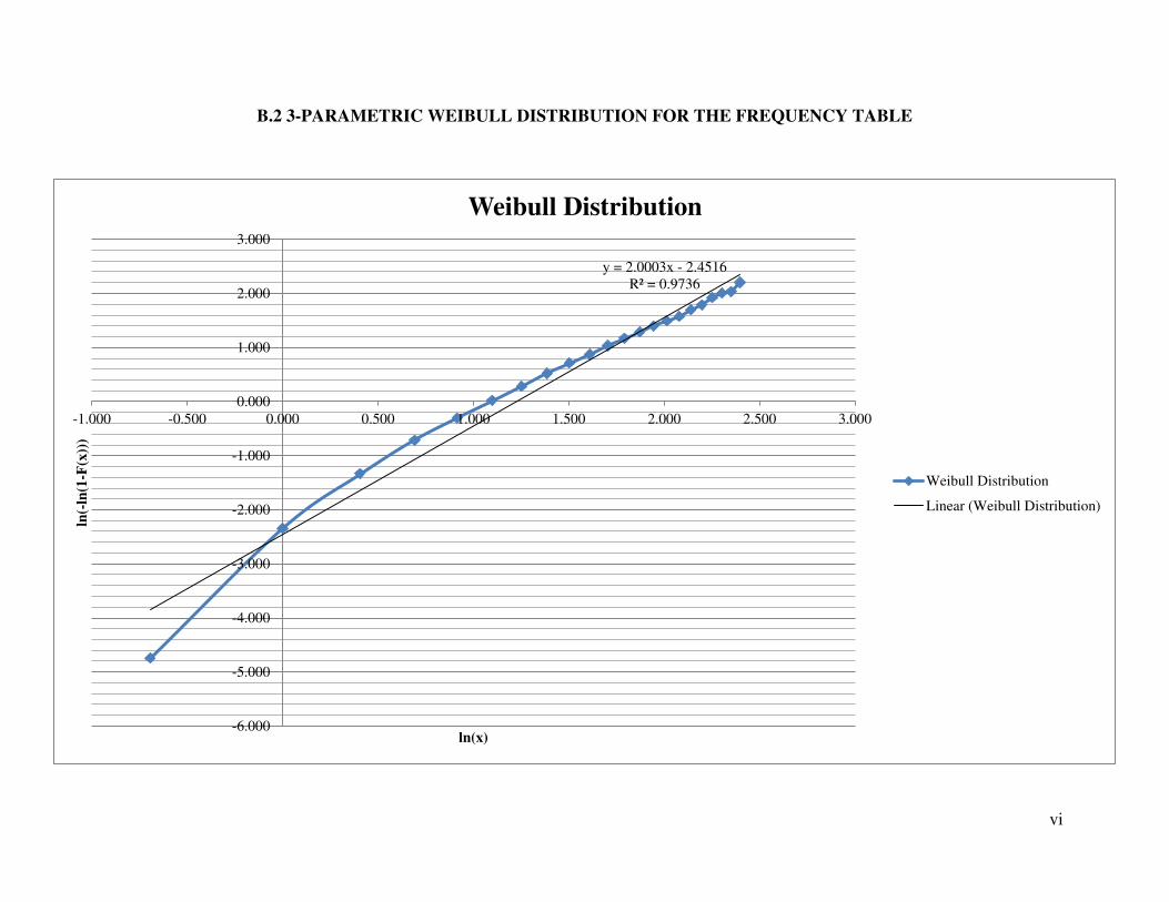
vi
B.2 3-PARAMETRIC WEIBULL DISTRIBUTION FOR THE FREQUENCY TABLE
y = 2.0003x - 2.4516
R² = 0.9736
-6.000
-5.000
-4.000
-3.000
-2.000
-1.000
0.000
1.000
2.000
3.000
-1.000 -0.500 0.000 0.500 1.000 1.500 2.000 2.500 3.000
ln(-
ln(1
-F(x
)))
ln(x)
Weibull Distribution
Weibull Distribution
Linear (Weibull Distribution)
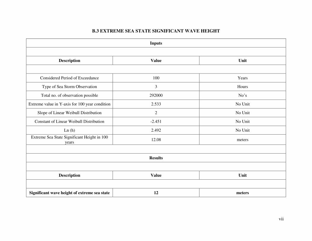
vii
B.3 EXTREME SEA STATE SIGNIFICANT WAVE HEIGHT
Inputs
Description Value Unit
Considered Period of Exceedance 100 Years
Type of Sea Storm Observation 3 Hours
Total no. of observation possible 292000 No’s
Extreme value in Y-axis for 100 year condition 2.533 No Unit
Slope of Linear Weibull Distribution 2 No Unit
Constant of Linear Weibull Distribution -2.451 No Unit
Ln (h) 2.492 No Unit
Extreme Sea State Significant Height in 100
years 12.08 meters
Results
Description Value Unit
Significant wave height of extreme sea state 12 meters
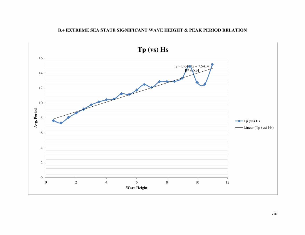
viii
B.4 EXTREME SEA STATE SIGNIFICANT WAVE HEIGHT & PEAK PERIOD RELATION
y = 0.6457x + 7.5414
R² = 0.91
0
2
4
6
8
10
12
14
16
0 2 4 6 8 10 12
Av
g. P
erio
d
Wave Height
Tp (vs) Hs
Tp (vs) Hs
Linear (Tp (vs) Hs)
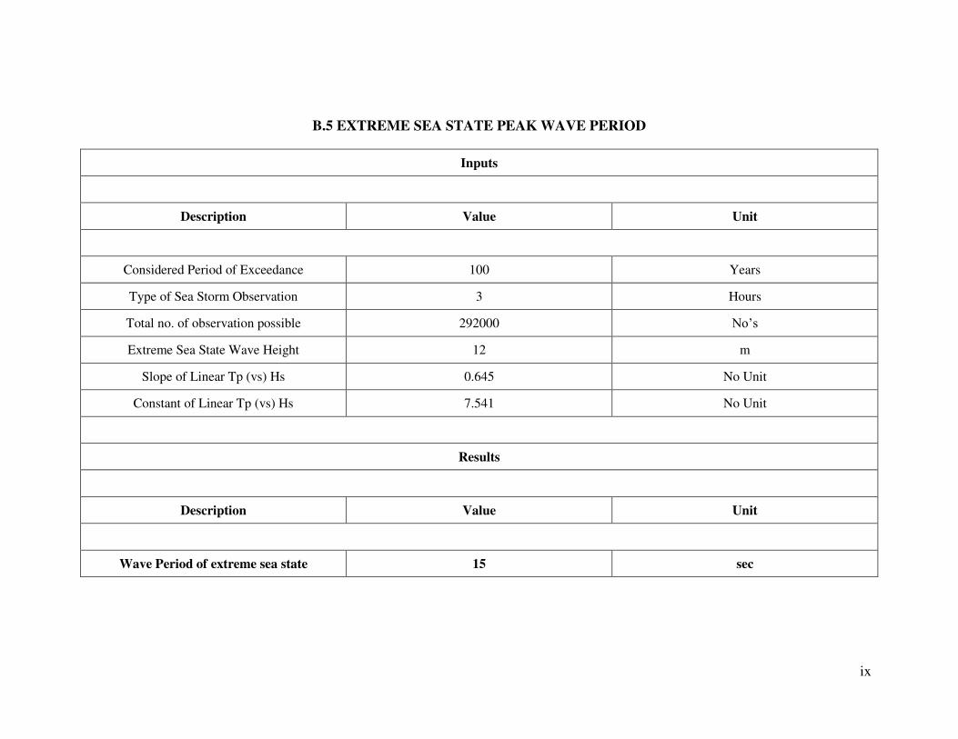
ix
B.5 EXTREME SEA STATE PEAK WAVE PERIOD
Inputs
Description Value Unit
Considered Period of Exceedance 100 Years
Type of Sea Storm Observation 3 Hours
Total no. of observation possible 292000 No’s
Extreme Sea State Wave Height 12 m
Slope of Linear Tp (vs) Hs 0.645 No Unit
Constant of Linear Tp (vs) Hs 7.541 No Unit
Results
Description Value Unit
Wave Period of extreme sea state 15 sec
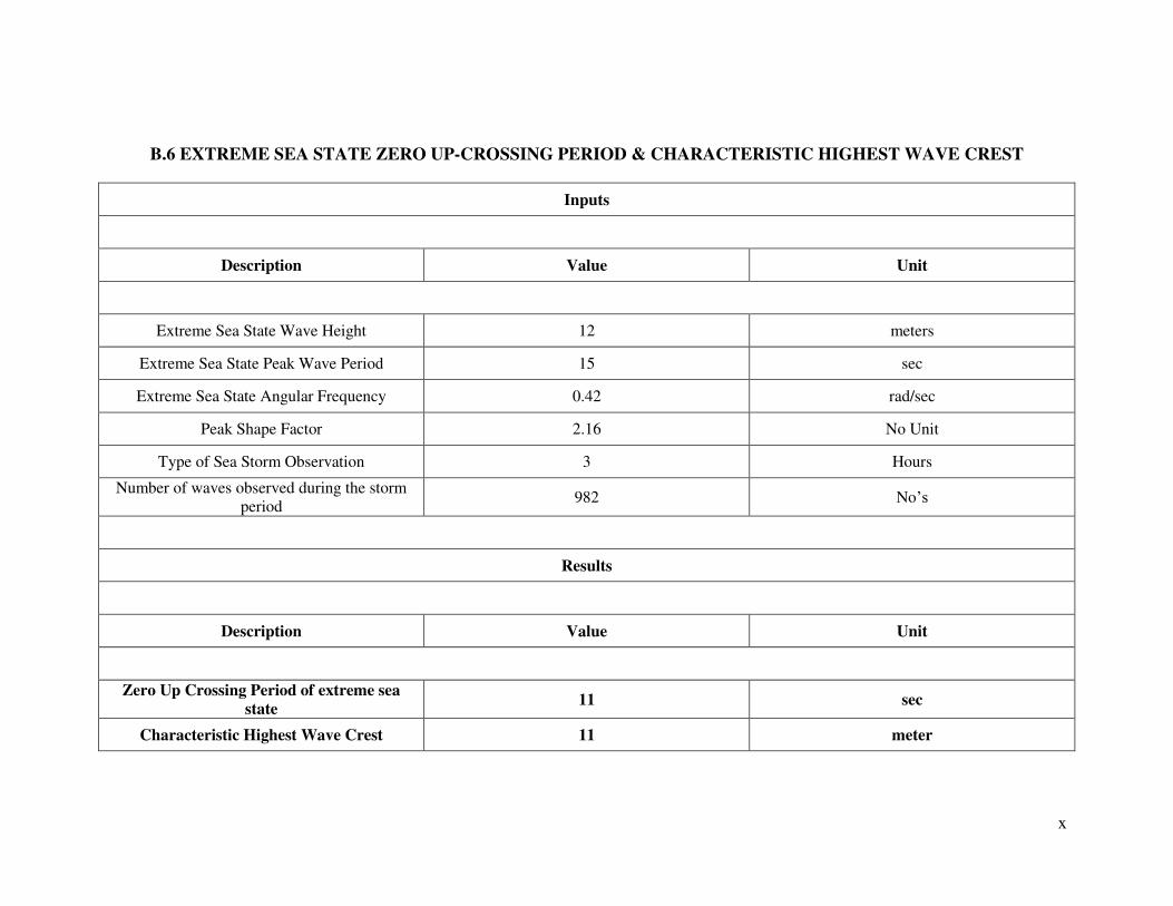
x
B.6 EXTREME SEA STATE ZERO UP-CROSSING PERIOD & CHARACTERISTIC HIGHEST WAVE CREST
Inputs
Description Value Unit
Extreme Sea State Wave Height 12 meters
Extreme Sea State Peak Wave Period 15 sec
Extreme Sea State Angular Frequency 0.42 rad/sec
Peak Shape Factor 2.16 No Unit
Type of Sea Storm Observation 3 Hours
Number of waves observed during the storm
period 982 No’s
Results
Description Value Unit
Zero Up Crossing Period of extreme sea
state 11 sec
Characteristic Highest Wave Crest 11 meter
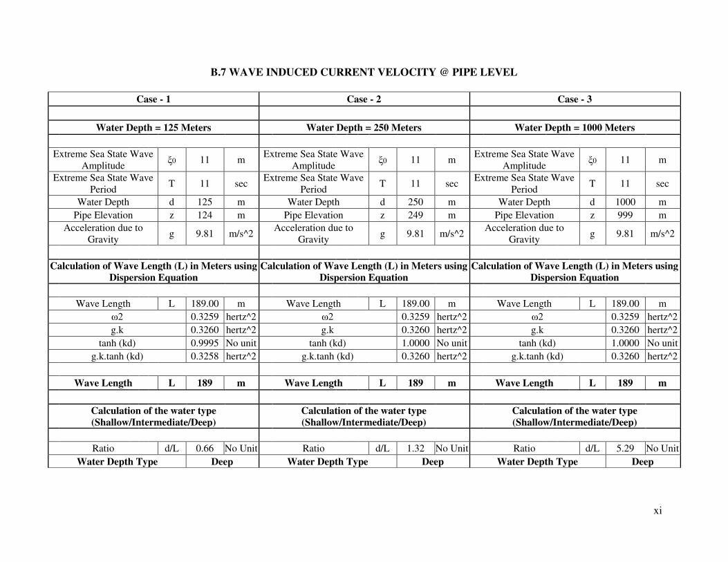
xi
B.7 WAVE INDUCED CURRENT VELOCITY @ PIPE LEVEL
Case - 1 Case - 2 Case - 3
Water Depth = 125 Meters Water Depth = 250 Meters Water Depth = 1000 Meters
Extreme Sea State Wave
Amplitude ξ0 11 m
Extreme Sea State Wave
Amplitude ξ0 11 m
Extreme Sea State Wave
Amplitude ξ0 11 m
Extreme Sea State Wave
Period T 11 sec
Extreme Sea State Wave
Period T 11 sec
Extreme Sea State Wave
Period T 11 sec
Water Depth d 125 m Water Depth d 250 m Water Depth d 1000 m
Pipe Elevation z 124 m Pipe Elevation z 249 m Pipe Elevation z 999 m
Acceleration due to
Gravity g 9.81 m/s^2
Acceleration due to
Gravity g 9.81 m/s^2
Acceleration due to
Gravity g 9.81 m/s^2
Calculation of Wave Length (L) in Meters using
Dispersion Equation
Calculation of Wave Length (L) in Meters using
Dispersion Equation
Calculation of Wave Length (L) in Meters using
Dispersion Equation
Wave Length L 189.00 m Wave Length L 189.00 m Wave Length L 189.00 m
ω2 0.3259 hertz^2 ω2 0.3259 hertz^2 ω2 0.3259 hertz^2
g.k 0.3260 hertz^2 g.k 0.3260 hertz^2 g.k 0.3260 hertz^2
tanh (kd) 0.9995 No unit tanh (kd) 1.0000 No unit tanh (kd) 1.0000 No unit
g.k.tanh (kd) 0.3258 hertz^2 g.k.tanh (kd) 0.3260 hertz^2 g.k.tanh (kd) 0.3260 hertz^2
Wave Length L 189 m Wave Length L 189 m Wave Length L 189 m
Calculation of the water type
(Shallow/Intermediate/Deep)
Calculation of the water type
(Shallow/Intermediate/Deep)
Calculation of the water type
(Shallow/Intermediate/Deep)
Ratio d/L 0.66 No Unit Ratio d/L 1.32 No Unit Ratio d/L 5.29 No Unit
Water Depth Type Deep Water Depth Type Deep Water Depth Type Deep
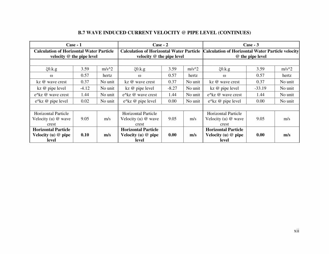
xii
B.7 WAVE INDUCED CURRENT VELOCITY @ PIPE LEVEL (CONTINUES)
Case - 1 Case - 2 Case - 3
Calculation of Horizontal Water Particle
velocity @ the pipe level
Calculation of Horizontal Water Particle
velocity @ the pipe level
Calculation of Horizontal Water Particle velocity
@ the pipe level
ξ0.k.g 3.59 m/s^2 ξ0.k.g 3.59 m/s^2 ξ0.k.g 3.59 m/s^2
ω 0.57 hertz ω 0.57 hertz ω 0.57 hertz
kz @ wave crest 0.37 No unit kz @ wave crest 0.37 No unit kz @ wave crest 0.37 No unit
kz @ pipe level -4.12 No unit kz @ pipe level -8.27 No unit kz @ pipe level -33.19 No unit
e^kz @ wave crest 1.44 No unit e^kz @ wave crest 1.44 No unit e^kz @ wave crest 1.44 No unit
e^kz @ pipe level 0.02 No unit e^kz @ pipe level 0.00 No unit e^kz @ pipe level 0.00 No unit
Horizontal Particle
Velocity (u) @ wave
crest
9.05 m/s
Horizontal Particle
Velocity (u) @ wave
crest
9.05 m/s
Horizontal Particle
Velocity (u) @ wave
crest
9.05 m/s
Horizontal Particle
Velocity (u) @ pipe
level
0.10 m/s
Horizontal Particle
Velocity (u) @ pipe
level
0.00 m/s
Horizontal Particle
Velocity (u) @ pipe
level
0.00 m/s
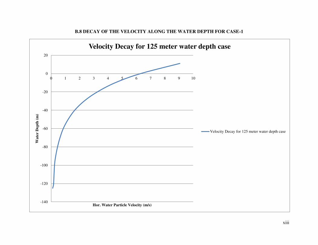
xiii
B.8 DECAY OF THE VELOCITY ALONG THE WATER DEPTH FOR CASE-1
-140
-120
-100
-80
-60
-40
-20
0
20
0 1 2 3 4 5 6 7 8 9 10
Wa
ter
Dep
th (
m)
Hor. Water Particle Velocity (m/s)
Velocity Decay for 125 meter water depth case
Velocity Decay for 125 meter water depth case
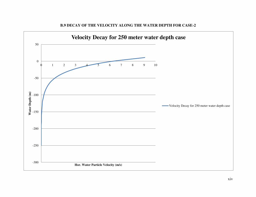
xiv
B.9 DECAY OF THE VELOCITY ALONG THE WATER DEPTH FOR CASE-2
-300
-250
-200
-150
-100
-50
0
50
0 1 2 3 4 5 6 7 8 9 10
Wa
ter
Dep
th (
m)
Hor. Water Particle Velocity (m/s)
Velocity Decay for 250 meter water depth case
Velocity Decay for 250 meter water depth case
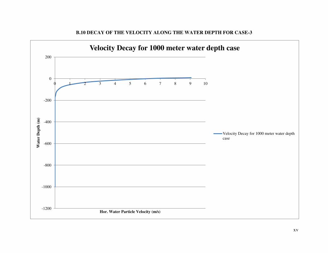
xv
B.10 DECAY OF THE VELOCITY ALONG THE WATER DEPTH FOR CASE-3
-1200
-1000
-800
-600
-400
-200
0
200
0 1 2 3 4 5 6 7 8 9 10
Wa
ter
Dep
th (
m)
Hor. Water Particle Velocity (m/s)
Velocity Decay for 1000 meter water depth case
Velocity Decay for 1000 meter water depth
case
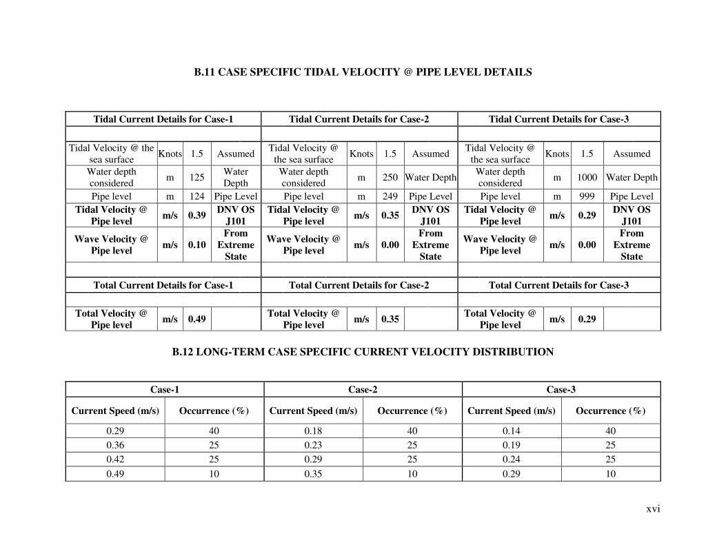
xvi
B.11 CASE SPECIFIC TIDAL VELOCITY @ PIPE LEVEL DETAILS
Tidal Current Details for Case-1 Tidal Current Details for Case-2 Tidal Current Details for Case-3
Tidal Velocity @ the
sea surface Knots 1.5 Assumed
Tidal Velocity @
the sea surface Knots 1.5 Assumed
Tidal Velocity @
the sea surface Knots 1.5 Assumed
Water depth
considered m 125
Water
Depth
Water depth
considered m 250 Water Depth
Water depth
considered m 1000 Water Depth
Pipe level m 124 Pipe Level Pipe level m 249 Pipe Level Pipe level m 999 Pipe Level
Tidal Velocity @
Pipe level m/s 0.39
DNV OS
J101
Tidal Velocity @
Pipe level m/s 0.35
DNV OS
J101
Tidal Velocity @
Pipe level m/s 0.29
DNV OS
J101
Wave Velocity @
Pipe level m/s 0.10
From
Extreme
State
Wave Velocity @
Pipe level m/s 0.00
From
Extreme
State
Wave Velocity @
Pipe level m/s 0.00
From
Extreme
State
Total Current Details for Case-1 Total Current Details for Case-2 Total Current Details for Case-3
Total Velocity @
Pipe level m/s 0.49
Total Velocity @
Pipe level m/s 0.35
Total Velocity @
Pipe level m/s 0.29
B.12 LONG-TERM CASE SPECIFIC CURRENT VELOCITY DISTRIBUTION
Case-1 Case-2 Case-3
Current Speed (m/s) Occurrence (%) Current Speed (m/s) Occurrence (%) Current Speed (m/s) Occurrence (%)
0.29 40 0.18 40 0.14 40
0.36 25 0.23 25 0.19 25
0.42 25 0.29 25 0.24 25
0.49 10 0.35 10 0.29 10
ANNEXURE – C
RESPONSE MODELLING
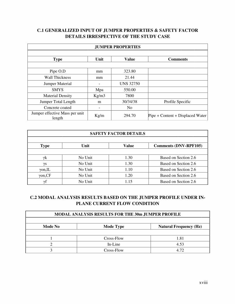
xviii
C.1 GENERALIZED INPUT OF JUMPER PROPERTIES & SAFETY FACTOR
DETAILS IRRESPECTIVE OF THE STUDY CASE
C.2 MODAL ANALYSIS RESULTS BASED ON THE JUMPER PROFILE UNDER IN-
PLANE CURRENT FLOW CONDITION
JUMPER PROPERTIES
Type Unit Value Comments
Pipe O.D mm 323.80
Wall Thickness mm 21.44
Jumper Material - UNS 32750
SMYS Mpa 550.00
Material Density Kg/m3 7800
Jumper Total Length m 30/34/38 Profile Specific
Concrete coated - No
Jumper effective Mass per unit
length Kg/m 294.70 Pipe + Content + Displaced Water
SAFETY FACTOR DETAILS
Type Unit Value Comments (DNV-RPF105)
γk No Unit 1.30 Based on Section 2.6
γs No Unit 1.30 Based on Section 2.6
γon,IL No Unit 1.10 Based on Section 2.6
γon,CF No Unit 1.20 Based on Section 2.6
γf No Unit 1.15 Based on Section 2.6
MODAL ANALYSIS RESULTS FOR THE 30m JUMPER PROFILE
Mode No Mode Type Natural Frequency (Hz)
1 Cross-Flow 1.81
2 In-Line 4.53
3 Cross-Flow 4.72
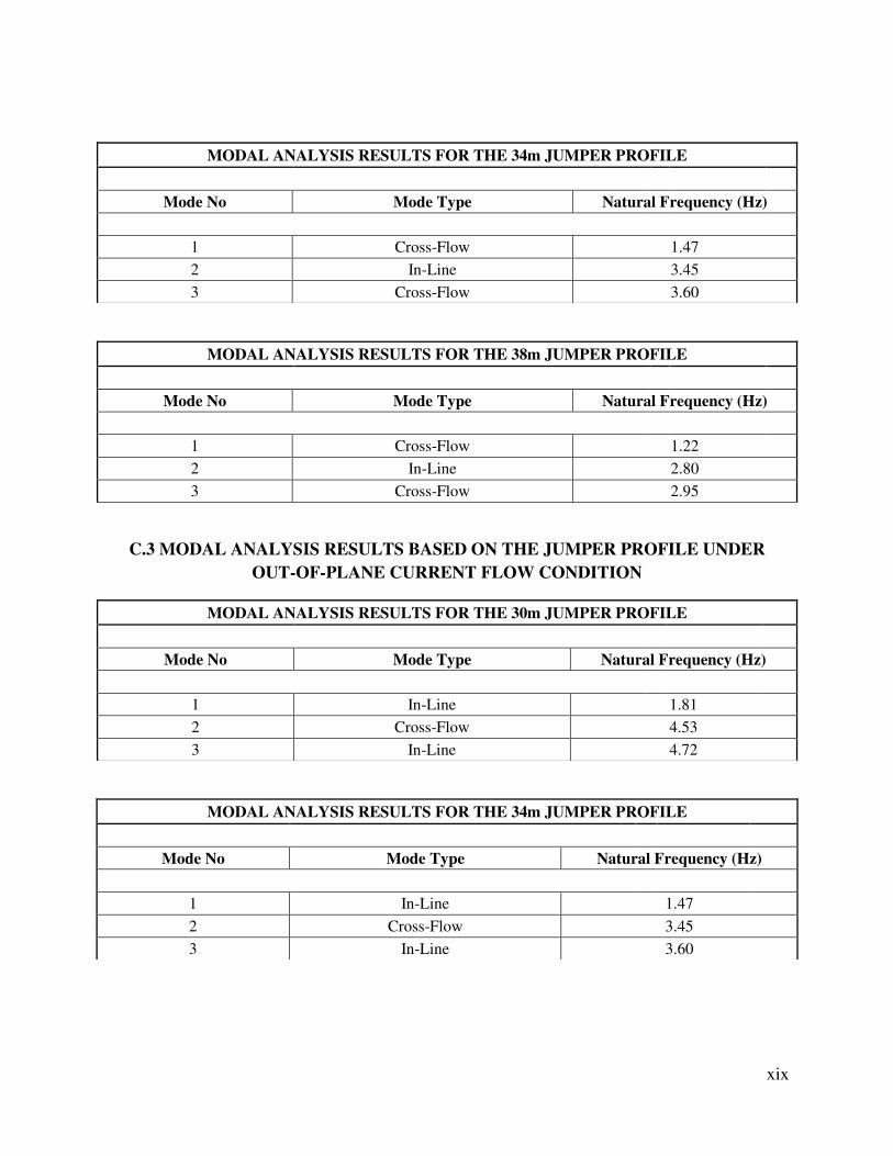
xix
C.3 MODAL ANALYSIS RESULTS BASED ON THE JUMPER PROFILE UNDER
OUT-OF-PLANE CURRENT FLOW CONDITION
MODAL ANALYSIS RESULTS FOR THE 34m JUMPER PROFILE
Mode No Mode Type Natural Frequency (Hz)
1 Cross-Flow 1.47
2 In-Line 3.45
3 Cross-Flow 3.60
MODAL ANALYSIS RESULTS FOR THE 38m JUMPER PROFILE
Mode No Mode Type Natural Frequency (Hz)
1 Cross-Flow 1.22
2 In-Line 2.80
3 Cross-Flow 2.95
MODAL ANALYSIS RESULTS FOR THE 30m JUMPER PROFILE
Mode No Mode Type Natural Frequency (Hz)
1 In-Line 1.81
2 Cross-Flow 4.53
3 In-Line 4.72
MODAL ANALYSIS RESULTS FOR THE 34m JUMPER PROFILE
Mode No Mode Type Natural Frequency (Hz)
1 In-Line 1.47
2 Cross-Flow 3.45
3 In-Line 3.60
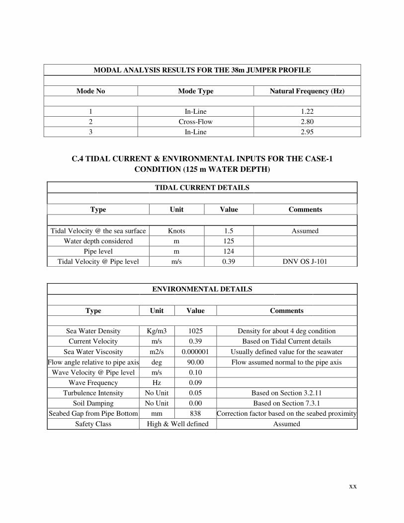
xx
C.4 TIDAL CURRENT & ENVIRONMENTAL INPUTS FOR THE CASE-1
CONDITION (125 m WATER DEPTH)
MODAL ANALYSIS RESULTS FOR THE 38m JUMPER PROFILE
Mode No Mode Type Natural Frequency (Hz)
1 In-Line 1.22
2 Cross-Flow 2.80
3 In-Line 2.95
TIDAL CURRENT DETAILS
Type Unit Value Comments
Tidal Velocity @ the sea surface Knots 1.5 Assumed
Water depth considered m 125
Pipe level m 124
Tidal Velocity @ Pipe level m/s 0.39 DNV OS J-101
ENVIRONMENTAL DETAILS
Type Unit Value Comments
Sea Water Density Kg/m3 1025 Density for about 4 deg condition
Current Velocity m/s 0.39 Based on Tidal Current details
Sea Water Viscosity m2/s 0.000001 Usually defined value for the seawater
Flow angle relative to pipe axis deg 90.00 Flow assumed normal to the pipe axis
Wave Velocity @ Pipe level m/s 0.10
Wave Frequency Hz 0.09
Turbulence Intensity No Unit 0.05 Based on Section 3.2.11
Soil Damping No Unit 0.00 Based on Section 7.3.1
Seabed Gap from Pipe Bottom mm 838 Correction factor based on the seabed proximity
Safety Class High & Well defined Assumed
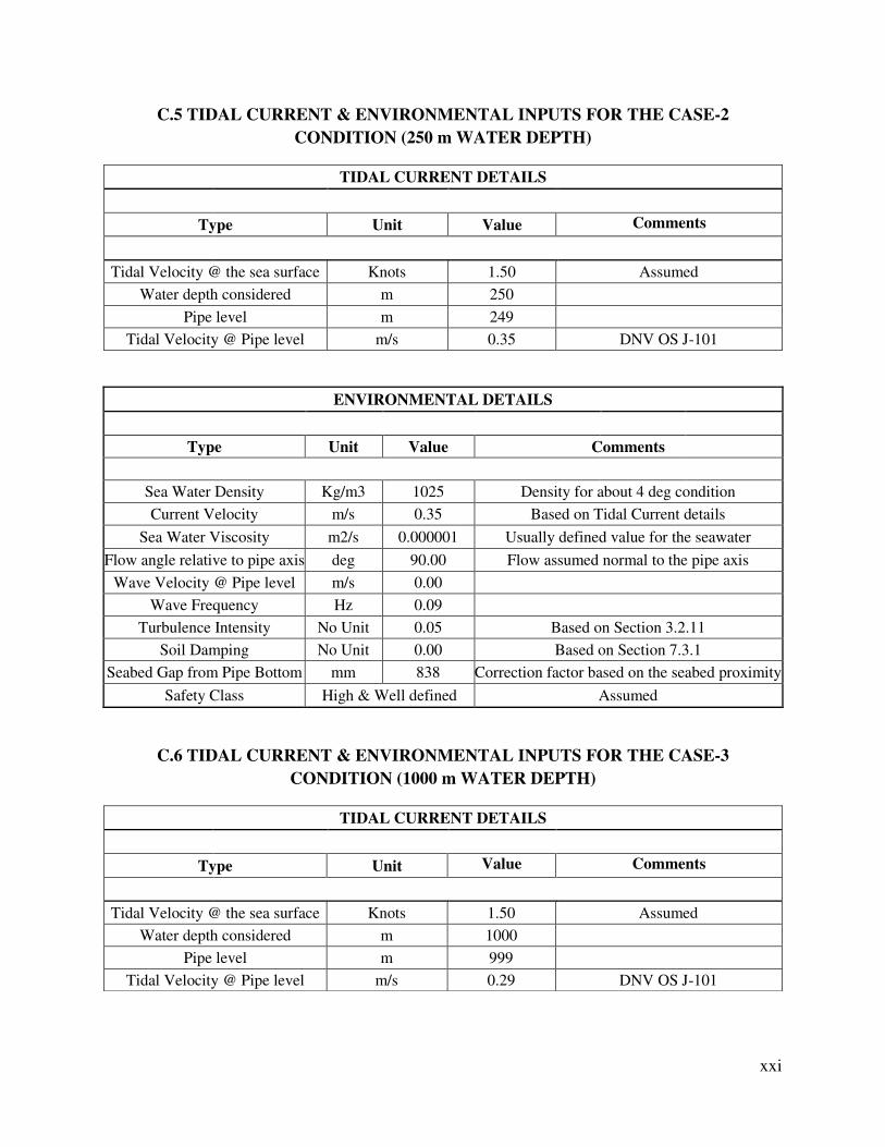
xxi
C.5 TIDAL CURRENT & ENVIRONMENTAL INPUTS FOR THE CASE-2
CONDITION (250 m WATER DEPTH)
C.6 TIDAL CURRENT & ENVIRONMENTAL INPUTS FOR THE CASE-3
CONDITION (1000 m WATER DEPTH)
TIDAL CURRENT DETAILS
Type Unit Value Comments
Tidal Velocity @ the sea surface Knots 1.50 Assumed
Water depth considered m 250
Pipe level m 249
Tidal Velocity @ Pipe level m/s 0.35 DNV OS J-101
ENVIRONMENTAL DETAILS
Type Unit Value Comments
Sea Water Density Kg/m3 1025 Density for about 4 deg condition
Current Velocity m/s 0.35 Based on Tidal Current details
Sea Water Viscosity m2/s 0.000001 Usually defined value for the seawater
Flow angle relative to pipe axis deg 90.00 Flow assumed normal to the pipe axis
Wave Velocity @ Pipe level m/s 0.00
Wave Frequency Hz 0.09
Turbulence Intensity No Unit 0.05 Based on Section 3.2.11
Soil Damping No Unit 0.00 Based on Section 7.3.1
Seabed Gap from Pipe Bottom mm 838 Correction factor based on the seabed proximity
Safety Class High & Well defined Assumed
TIDAL CURRENT DETAILS
Type Unit Value Comments
Tidal Velocity @ the sea surface Knots 1.50 Assumed
Water depth considered m 1000
Pipe level m 999
Tidal Velocity @ Pipe level m/s 0.29 DNV OS J-101
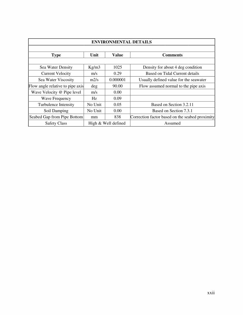
xxii
ENVIRONMENTAL DETAILS
Type Unit Value Comments
Sea Water Density Kg/m3 1025 Density for about 4 deg condition
Current Velocity m/s 0.29 Based on Tidal Current details
Sea Water Viscosity m2/s 0.000001 Usually defined value for the seawater
Flow angle relative to pipe axis deg 90.00 Flow assumed normal to the pipe axis
Wave Velocity @ Pipe level m/s 0.00
Wave Frequency Hz 0.09
Turbulence Intensity No Unit 0.05 Based on Section 3.2.11
Soil Damping No Unit 0.00 Based on Section 7.3.1
Seabed Gap from Pipe Bottom mm 838 Correction factor based on the seabed proximity
Safety Class High & Well defined Assumed
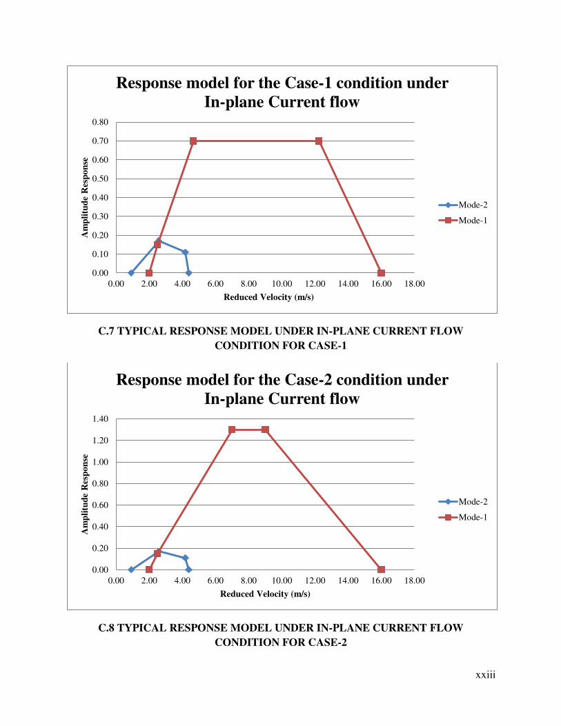
xxiii
C.7 TYPICAL RESPONSE MODEL UNDER IN-PLANE CURRENT FLOW
CONDITION FOR CASE-1
C.8 TYPICAL RESPONSE MODEL UNDER IN-PLANE CURRENT FLOW
CONDITION FOR CASE-2
0.00
0.10
0.20
0.30
0.40
0.50
0.60
0.70
0.80
0.00 2.00 4.00 6.00 8.00 10.00 12.00 14.00 16.00 18.00
Am
pli
tud
e R
esp
on
se
Reduced Velocity (m/s)
Response model for the Case-1 condition under
In-plane Current flow
Mode-2
Mode-1
0.00
0.20
0.40
0.60
0.80
1.00
1.20
1.40
0.00 2.00 4.00 6.00 8.00 10.00 12.00 14.00 16.00 18.00
Am
pli
tud
e R
esp
on
se
Reduced Velocity (m/s)
Response model for the Case-2 condition under
In-plane Current flow
Mode-2
Mode-1
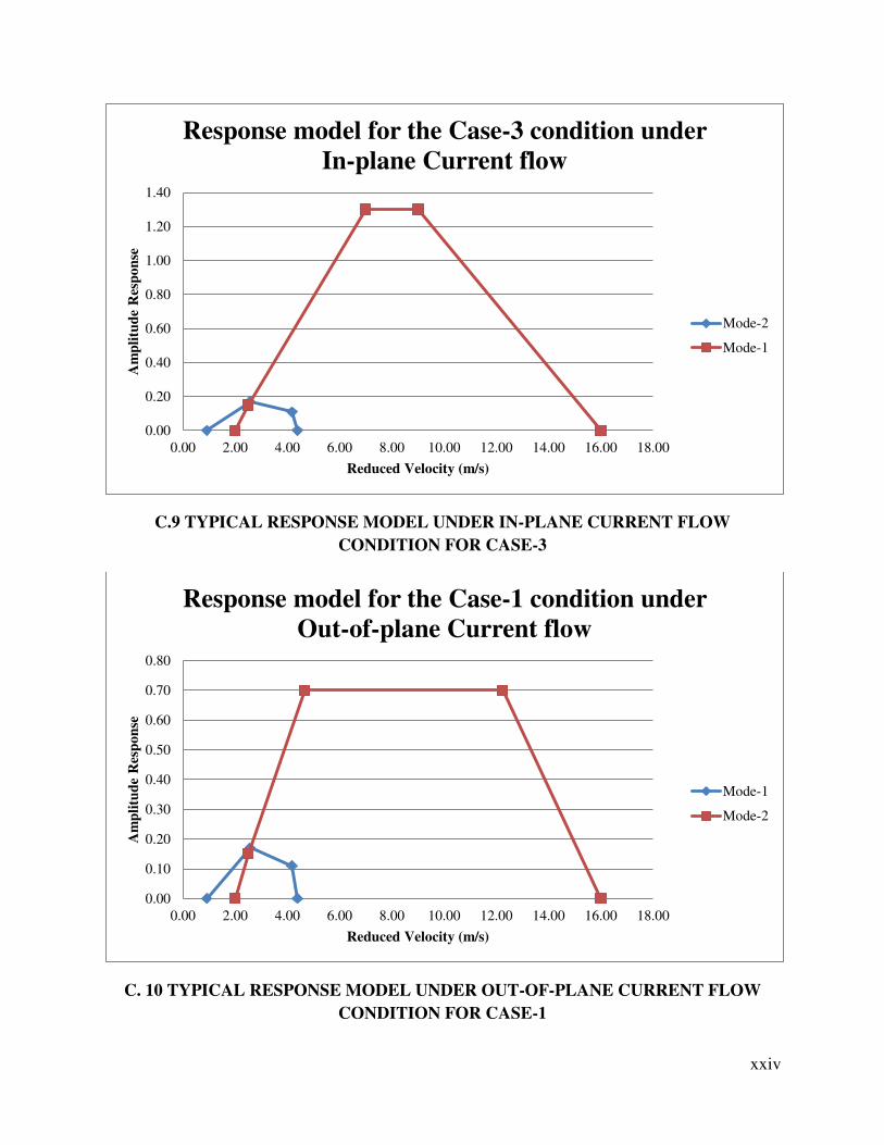
xxiv
C.9 TYPICAL RESPONSE MODEL UNDER IN-PLANE CURRENT FLOW
CONDITION FOR CASE-3
C. 10 TYPICAL RESPONSE MODEL UNDER OUT-OF-PLANE CURRENT FLOW
CONDITION FOR CASE-1
0.00
0.20
0.40
0.60
0.80
1.00
1.20
1.40
0.00 2.00 4.00 6.00 8.00 10.00 12.00 14.00 16.00 18.00
Am
pli
tud
e R
esp
on
se
Reduced Velocity (m/s)
Response model for the Case-3 condition under
In-plane Current flow
Mode-2
Mode-1
0.00
0.10
0.20
0.30
0.40
0.50
0.60
0.70
0.80
0.00 2.00 4.00 6.00 8.00 10.00 12.00 14.00 16.00 18.00
Am
pli
tud
e R
esp
on
se
Reduced Velocity (m/s)
Response model for the Case-1 condition under
Out-of-plane Current flow
Mode-1
Mode-2
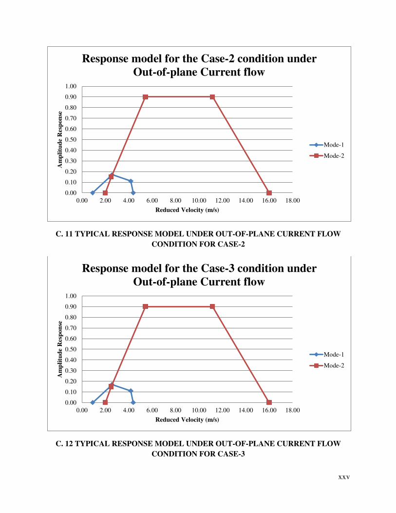
xxv
C. 11 TYPICAL RESPONSE MODEL UNDER OUT-OF-PLANE CURRENT FLOW
CONDITION FOR CASE-2
C. 12 TYPICAL RESPONSE MODEL UNDER OUT-OF-PLANE CURRENT FLOW
CONDITION FOR CASE-3
0.00
0.10
0.20
0.30
0.40
0.50
0.60
0.70
0.80
0.90
1.00
0.00 2.00 4.00 6.00 8.00 10.00 12.00 14.00 16.00 18.00
Am
pli
tud
e R
esp
on
se
Reduced Velocity (m/s)
Response model for the Case-2 condition under
Out-of-plane Current flow
Mode-1
Mode-2
0.00
0.10
0.20
0.30
0.40
0.50
0.60
0.70
0.80
0.90
1.00
0.00 2.00 4.00 6.00 8.00 10.00 12.00 14.00 16.00 18.00
Am
pli
tud
e R
esp
on
se
Reduced Velocity (m/s)
Response model for the Case-3 condition under
Out-of-plane Current flow
Mode-1
Mode-2
ANNEXURE – D
PROFILE SPECIFIC REDUCED VELOCITY (Vr)
VARIATION BASED ON THE PROBABILITY OF
THE SEABED CURRENT CONDITION

xxvii
D.1 REDUCED VELOCITY FOR 30 METER JUMPER CONFIGURATION UNDER CASE-1
Case Study Probability of
Occurrence
Seabed Current
Velocity Eigen Frequency Pipe Diameter Reduced Velocity
No's % m/s Hz m m/s
1
10 0.49
1.81
0.3238
0.84
4.53 0.33
4.72 0.32
25% type-1 0.42
1.81 0.72
4.53 0.29
4.72 0.27
25% type-2 0.36
1.81 0.61
4.53 0.25
4.72 0.24
40 0.29
1.81 0.49
4.53 0.20
4.72 0.19

xxviii
D.2 REDUCED VELOCITY FOR 30 METER JUMPER CONFIGURATION UNDER CASE-2
Case Study Probability of
Occurrence
Seabed Current
Velocity Eigen Frequency Pipe Diameter Reduced Velocity
No's % m/s Hz m m/s
2
10 0.35
1.81
0.3238
0.60
4.53 0.24
4.72 0.23
25% type-1 0.29
1.81 0.49
4.53 0.20
4.72 0.19
25% type-2 0.23
1.81 0.39
4.53 0.16
4.72 0.15
40 0.18
1.81 0.31
4.53 0.12
4.72 0.12
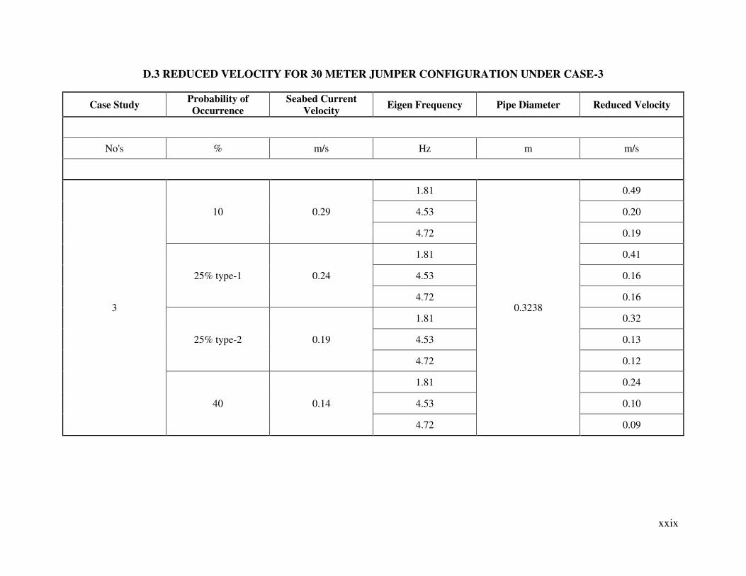
xxix
D.3 REDUCED VELOCITY FOR 30 METER JUMPER CONFIGURATION UNDER CASE-3
Case Study Probability of
Occurrence
Seabed Current
Velocity Eigen Frequency Pipe Diameter Reduced Velocity
No's % m/s Hz m m/s
3
10 0.29
1.81
0.3238
0.49
4.53 0.20
4.72 0.19
25% type-1 0.24
1.81 0.41
4.53 0.16
4.72 0.16
25% type-2 0.19
1.81 0.32
4.53 0.13
4.72 0.12
40 0.14
1.81 0.24
4.53 0.10
4.72 0.09

xxx
D.4 REDUCED VELOCITY FOR 34 METER JUMPER CONFIGURATION UNDER CASE-1
Case Study Probability of
Occurrence
Seabed Current
Velocity Eigen Frequency Pipe Diameter Reduced Velocity
No's % m/s Hz m m/s
1
10 0.49
1.47
0.3238
1.03
3.45 0.44
3.6 0.42
25% type-1 0.42
1.47 0.88
3.46 0.37
3.6 0.36
25% type-2 0.36
1.47 0.76
3.46 0.32
3.6 0.31
40 0.29
1.47 0.61
3.45 0.26
3.6 0.25
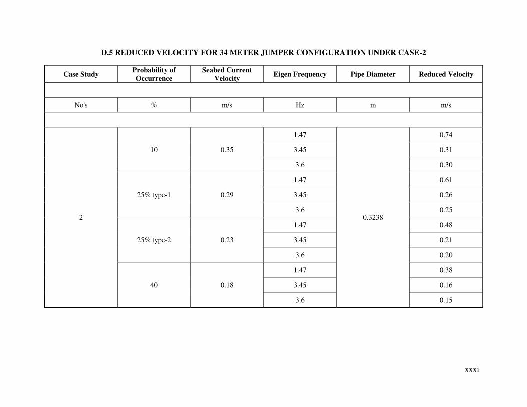
xxxi
D.5 REDUCED VELOCITY FOR 34 METER JUMPER CONFIGURATION UNDER CASE-2
Case Study Probability of
Occurrence
Seabed Current
Velocity Eigen Frequency Pipe Diameter Reduced Velocity
No's % m/s Hz m m/s
2
10 0.35
1.47
0.3238
0.74
3.45 0.31
3.6 0.30
25% type-1 0.29
1.47 0.61
3.45 0.26
3.6 0.25
25% type-2 0.23
1.47 0.48
3.45 0.21
3.6 0.20
40 0.18
1.47 0.38
3.45 0.16
3.6 0.15

xxxii
D.6 REDUCED VELOCITY FOR 34 METER JUMPER CONFIGURATION UNDER CASE-3
Case Study Probability of
Occurrence
Seabed Current
Velocity Eigen Frequency Pipe Diameter Reduced Velocity
No's % m/s Hz m m/s
3
10 0.29
1.47
0.3238
0.61
3.45 0.26
3.6 0.25
25% type-1 0.24
1.47 0.50
3.45 0.21
3.6 0.21
25% type-2 0.19
1.47 0.40
3.45 0.17
3.6 0.16
40 0.14
1.47 0.29
3.45 0.13
3.6 0.12
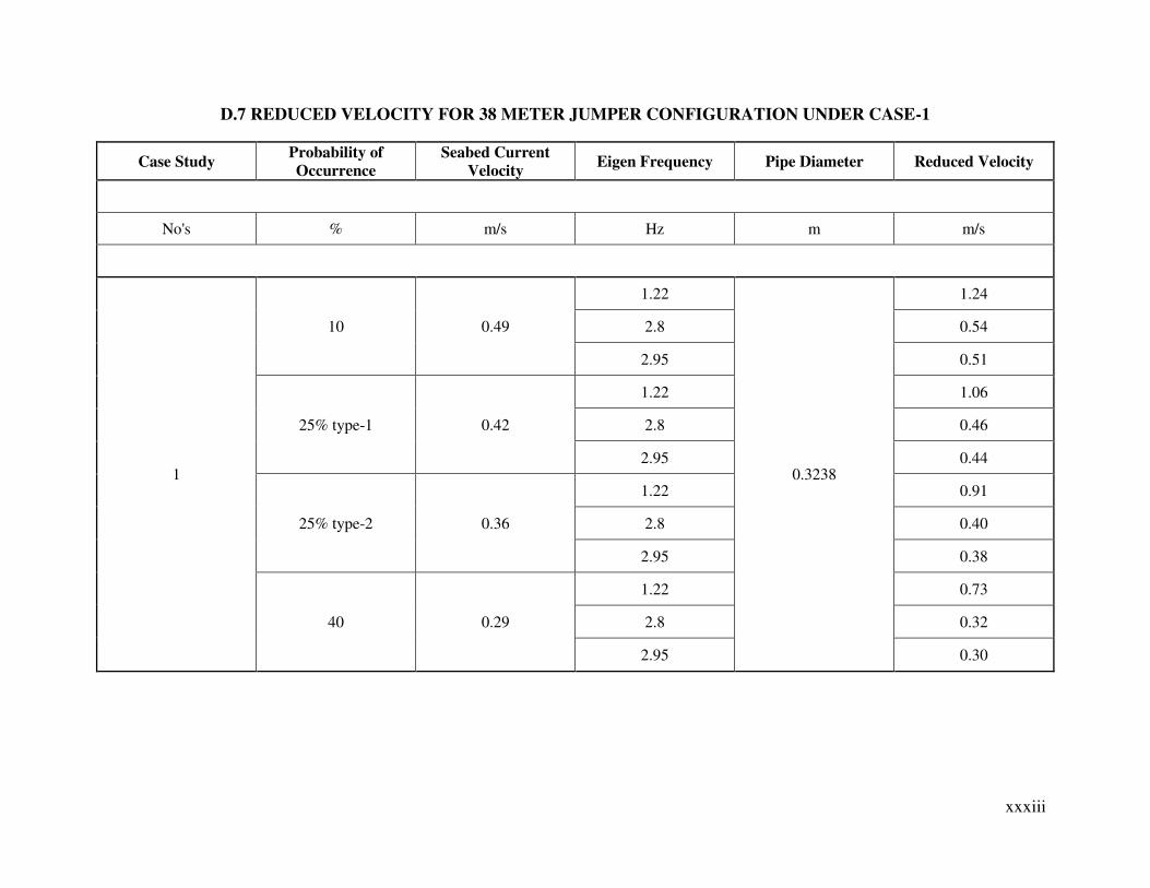
xxxiii
D.7 REDUCED VELOCITY FOR 38 METER JUMPER CONFIGURATION UNDER CASE-1
Case Study Probability of
Occurrence
Seabed Current
Velocity Eigen Frequency Pipe Diameter Reduced Velocity
No's % m/s Hz m m/s
1
10 0.49
1.22
0.3238
1.24
2.8 0.54
2.95 0.51
25% type-1 0.42
1.22 1.06
2.8 0.46
2.95 0.44
25% type-2 0.36
1.22 0.91
2.8 0.40
2.95 0.38
40 0.29
1.22 0.73
2.8 0.32
2.95 0.30
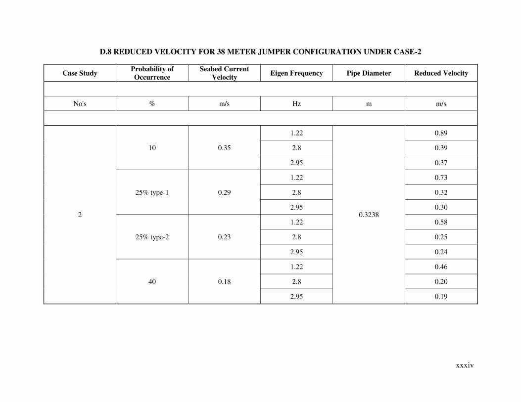
xxxiv
D.8 REDUCED VELOCITY FOR 38 METER JUMPER CONFIGURATION UNDER CASE-2
Case Study Probability of
Occurrence
Seabed Current
Velocity Eigen Frequency Pipe Diameter Reduced Velocity
No's % m/s Hz m m/s
2
10 0.35
1.22
0.3238
0.89
2.8 0.39
2.95 0.37
25% type-1 0.29
1.22 0.73
2.8 0.32
2.95 0.30
25% type-2 0.23
1.22 0.58
2.8 0.25
2.95 0.24
40 0.18
1.22 0.46
2.8 0.20
2.95 0.19

xxxv
D.9 REDUCED VELOCITY FOR 38 METER JUMPER CONFIGURATION UNDER CASE-3
Case Study Probability of
Occurrence
Seabed Current
Velocity Eigen Frequency Pipe Diameter Reduced Velocity
No's % m/s Hz m m/s
3
10 0.29
1.22
0.3238
0.73
2.8 0.32
2.95 0.30
25% type-1 0.24
1.22 0.61
2.8 0.26
2.95 0.25
25% type-2 0.19
1.22 0.48
2.8 0.21
2.95 0.20
40 0.14
1.22 0.35
2.8 0.15
2.95 0.15
ANNEXURE – E
FLOW SPECIFIC VIV “LOCK-IN” PHENOMENON CHECK
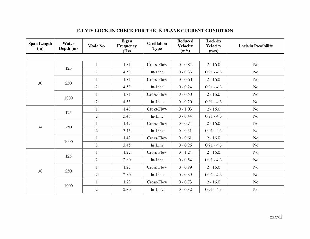
xxxvii
E.1 VIV LOCK-IN CHECK FOR THE IN-PLANE CURRENT CONDITION
Span Length
(m)
Water
Depth (m) Mode No.
Eigen
Frequency
(Hz)
Oscillation
Type
Reduced
Velocity
(m/s)
Lock-in
Velocity
(m/s)
Lock-in Possibility
30
125 1 1.81 Cross-Flow 0 - 0.84 2 - 16.0 No
2 4.53 In-Line 0 - 0.33 0.91 - 4.3 No
250 1 1.81 Cross-Flow 0 - 0.60 2 - 16.0 No
2 4.53 In-Line 0 - 0.24 0.91 - 4.3 No
1000 1 1.81 Cross-Flow 0 - 0.50 2 - 16.0 No
2 4.53 In-Line 0 - 0.20 0.91 - 4.3 No
34
125 1 1.47 Cross-Flow 0 - 1.03 2 - 16.0 No
2 3.45 In-Line 0 - 0.44 0.91 - 4.3 No
250 1 1.47 Cross-Flow 0 - 0.74 2 - 16.0 No
2 3.45 In-Line 0 - 0.31 0.91 - 4.3 No
1000 1 1.47 Cross-Flow 0 - 0.61 2 - 16.0 No
2 3.45 In-Line 0 - 0.26 0.91 - 4.3 No
38
125 1 1.22 Cross-Flow 0 - 1.24 2 - 16.0 No
2 2.80 In-Line 0 - 0.54 0.91 - 4.3 No
250 1 1.22 Cross-Flow 0 - 0.89 2 - 16.0 No
2 2.80 In-Line 0 - 0.39 0.91 - 4.3 No
1000 1 1.22 Cross-Flow 0 - 0.73 2 - 16.0 No
2 2.80 In-Line 0 - 0.32 0.91 - 4.3 No
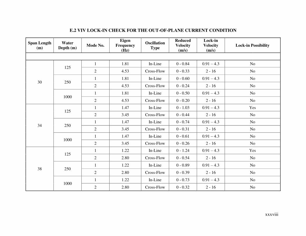
xxxviii
E.2 VIV LOCK-IN CHECK FOR THE OUT-OF-PLANE CURRENT CONDITION
Span Length
(m)
Water
Depth (m) Mode No.
Eigen
Frequency
(Hz)
Oscillation
Type
Reduced
Velocity
(m/s)
Lock-in
Velocity
(m/s)
Lock-in Possibility
30
125 1 1.81 In-Line 0 - 0.84 0.91 – 4.3 No
2 4.53 Cross-Flow 0 - 0.33 2 - 16 No
250 1 1.81 In-Line 0 - 0.60 0.91 – 4.3 No
2 4.53 Cross-Flow 0 - 0.24 2 - 16 No
1000 1 1.81 In-Line 0 - 0.50 0.91 – 4.3 No
2 4.53 Cross-Flow 0 - 0.20 2 - 16 No
34
125 1 1.47 In-Line 0 - 1.03 0.91 – 4.3 Yes
2 3.45 Cross-Flow 0 - 0.44 2 - 16 No
250 1 1.47 In-Line 0 - 0.74 0.91 – 4.3 No
2 3.45 Cross-Flow 0 - 0.31 2 - 16 No
1000 1 1.47 In-Line 0 - 0.61 0.91 – 4.3 No
2 3.45 Cross-Flow 0 - 0.26 2 - 16 No
38
125 1 1.22 In-Line 0 - 1.24 0.91 – 4.3 Yes
2 2.80 Cross-Flow 0 - 0.54 2 - 16 No
250 1 1.22 In-Line 0 - 0.89 0.91 – 4.3 No
2 2.80 Cross-Flow 0 - 0.39 2 - 16 No
1000 1 1.22 In-Line 0 - 0.73 0.91 – 4.3 No
2 2.80 Cross-Flow 0 - 0.32 2 - 16 No
ANNEXURE – F
CONFIGURATION SPECIFIC FATIGUE STRESS
RANGE EVALUATION
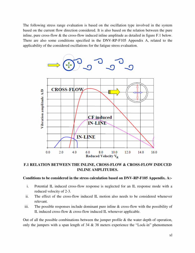
xl
The following stress range evaluation is based on the oscillation type involved in the system
based on the current flow direction considered. It is also based on the relation between the pure
inline, pure cross-flow & the cross-flow induced inline amplitude as detailed in figure F.1 below.
There are also some conditions specified in the DNV-RP-F105 Appendix A, related to the
applicability of the considered oscillations for the fatigue stress evaluation.
F.1 RELATION BETWEEN THE INLINE, CROSS-FLOW & CROSS-FLOW INDUCED
INLINE AMPLITUDES.
Conditions to be considered in the stress calculation based on DNV-RP-F105 Appendix. A:-
i. Potential IL induced cross-flow response is neglected for an IL response mode with a
reduced velocity of 2-3.
ii. The effect of the cross-flow induced IL motion also needs to be considered whenever
relevant.
iii. The possible responses include dominant pure inline & cross-flow with the possibility of
IL induced cross-flow & cross-flow induced IL whenever applicable.
Out of all the possible combinations between the jumper profile & the water depth of operation,
only the jumpers with a span length of 34 & 38 meters experience the “Lock-in” phenomenon
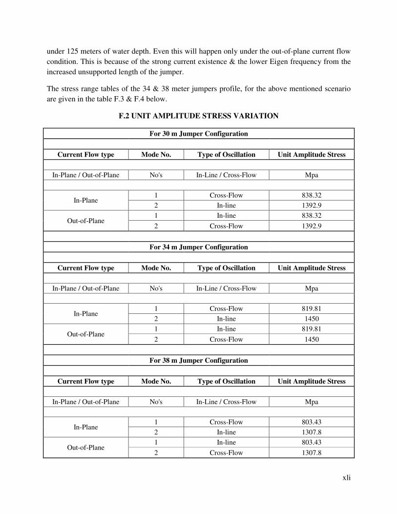
xli
under 125 meters of water depth. Even this will happen only under the out-of-plane current flow
condition. This is because of the strong current existence & the lower Eigen frequency from the
increased unsupported length of the jumper.
The stress range tables of the 34 & 38 meter jumpers profile, for the above mentioned scenario
are given in the table F.3 & F.4 below.
F.2 UNIT AMPLITUDE STRESS VARIATION
For 30 m Jumper Configuration
Current Flow type Mode No. Type of Oscillation Unit Amplitude Stress
In-Plane / Out-of-Plane No's In-Line / Cross-Flow Mpa
In-Plane 1 Cross-Flow 838.32
2 In-line 1392.9
Out-of-Plane 1 In-line 838.32
2 Cross-Flow 1392.9
For 34 m Jumper Configuration
Current Flow type Mode No. Type of Oscillation Unit Amplitude Stress
In-Plane / Out-of-Plane No's In-Line / Cross-Flow Mpa
In-Plane 1 Cross-Flow 819.81
2 In-line 1450
Out-of-Plane 1 In-line 819.81
2 Cross-Flow 1450
For 38 m Jumper Configuration
Current Flow type Mode No. Type of Oscillation Unit Amplitude Stress
In-Plane / Out-of-Plane No's In-Line / Cross-Flow Mpa
In-Plane 1 Cross-Flow 803.43
2 In-line 1307.8
Out-of-Plane 1 In-line 803.43
2 Cross-Flow 1307.8

xlii
F.3 EVALUATION OF STRESS RANGE FOR THE 34 m JUMPER UNDER OUT-OF-PLANE CURRENT
Amplitude Reduction Factor due to
Damping 0.9805 No Unit
Current Flow Ratio Correction Factor 0.986 No Unit
Safety Factor 1.3 No Unit Competing Modes Reduction Factor 1 No Unit
Span
Length
(m)
In-Line
Mode Unit
Stress
Amplitude
(Mpa)
Cross-Flow
Mode Unit
Stress
Amplitude
(Mpa)
Water
Depth (m)
Current
Velocity
(m/s)
Maximum
Inline VIV
Response
Amplitude
(No Unit)
Maximum
Cross-Flow
VIV
Response
Amplitude
(No Unit)
Stress
Range due
to pure
cross-flow
response
(Mpa)
Stress
Range due
to pure
inline
response
(Mpa)
Stress
Range due
to inline
induced
crossflow
response
(Mpa)
Total Stress
Range for
the
considered
case (Mpa)
34 819.81 1450 125
0.29 0 0 0 0 0 0
0.36 0 0 0 0 0 0
0.42 0 0 0 0 0 0
0.49 0.008 0 0 16.81 0 16.81
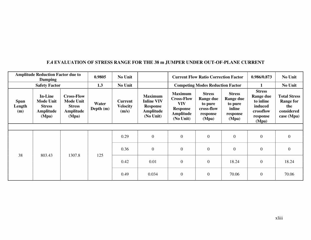
xliii
F.4 EVALUATION OF STRESS RANGE FOR THE 38 m JUMPER UNDER OUT-OF-PLANE CURRENT
Amplitude Reduction Factor due to
Damping 0.9805 No Unit
Current Flow Ratio Correction Factor 0.986/0.873 No Unit
Safety Factor 1.3 No Unit Competing Modes Reduction Factor 1 No Unit
Span
Length
(m)
In-Line
Mode Unit
Stress
Amplitude
(Mpa)
Cross-Flow
Mode Unit
Stress
Amplitude
(Mpa)
Water
Depth (m)
Current
Velocity
(m/s)
Maximum
Inline VIV
Response
Amplitude
(No Unit)
Maximum
Cross-Flow
VIV
Response
Amplitude
(No Unit)
Stress
Range due
to pure
cross-flow
response
(Mpa)
Stress
Range due
to pure
inline
response
(Mpa)
Stress
Range due
to inline
induced
crossflow
response
(Mpa)
Total Stress
Range for
the
considered
case (Mpa)
38 803.43 1307.8 125
0.29 0 0 0 0 0 0
0.36 0 0 0 0 0 0
0.42 0.01 0 0 18.24 0 18.24
0.49 0.034 0 0 70.06 0 70.06
ANNEXURE – G
CURRENT FLOW BASED EVALUATION OF THE
FATIGUE LIFE
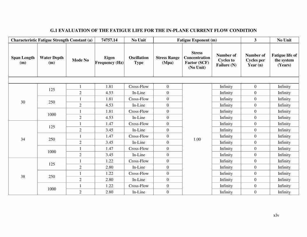
xlv
G.1 EVALUATION OF THE FATIGUE LIFE FOR THE IN-PLANE CURRENT FLOW CONDITION
Characteristic Fatigue Strength Constant (a) 74757.14 No Unit Fatigue Exponent (m) 3 No Unit
Span Length
(m)
Water Depth
(m) Mode No
Eigen
Frequency (Hz)
Oscillation
Type
Stress Range
(Mpa)
Stress
Concentration
Factor (SCF)
(No Unit)
Number of
Cycles to
Failure (N)
Number of
Cycles per
Year (n)
Fatigue life of
the system
(Years)
30
125 1 1.81 Cross-Flow 0
1.00
Infinity 0 Infinity
2 4.53 In-Line 0 Infinity 0 Infinity
250 1 1.81 Cross-Flow 0 Infinity 0 Infinity
2 4.53 In-Line 0 Infinity 0 Infinity
1000 1 1.81 Cross-Flow 0 Infinity 0 Infinity
2 4.53 In-Line 0 Infinity 0 Infinity
34
125 1 1.47 Cross-Flow 0 Infinity 0 Infinity
2 3.45 In-Line 0 Infinity 0 Infinity
250 1 1.47 Cross-Flow 0 Infinity 0 Infinity
2 3.45 In-Line 0 Infinity 0 Infinity
1000 1 1.47 Cross-Flow 0 Infinity 0 Infinity
2 3.45 In-Line 0 Infinity 0 Infinity
38
125 1 1.22 Cross-Flow 0 Infinity 0 Infinity
2 2.80 In-Line 0 Infinity 0 Infinity
250 1 1.22 Cross-Flow 0 Infinity 0 Infinity
2 2.80 In-Line 0 Infinity 0 Infinity
1000 1 1.22 Cross-Flow 0 Infinity 0 Infinity
2 2.80 In-Line 0 Infinity 0 Infinity
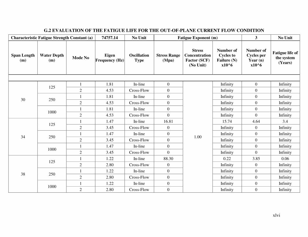
xlvi
G.2 EVALUATION OF THE FATIGUE LIFE FOR THE OUT-OF-PLANE CURRENT FLOW CONDITION
Characteristic Fatigue Strength Constant (a) 74757.14 No Unit Fatigue Exponent (m) 3 No Unit
Span Length
(m)
Water Depth
(m) Mode No
Eigen
Frequency (Hz)
Oscillation
Type
Stress Range
(Mpa)
Stress
Concentration
Factor (SCF)
(No Unit)
Number of
Cycles to
Failure (N)
x10^6
Number of
Cycles per
Year (n)
x10^6
Fatigue life of
the system
(Years)
30
125 1 1.81 In-line 0
1.00
Infinity 0 Infinity
2 4.53 Cross-Flow 0 Infinity 0 Infinity
250 1 1.81 In-line 0 Infinity 0 Infinity
2 4.53 Cross-Flow 0 Infinity 0 Infinity
1000 1 1.81 In-line 0 Infinity 0 Infinity
2 4.53 Cross-Flow 0 Infinity 0 Infinity
34
125 1 1.47 In-line 16.81 15.74 4.64 3.4
2 3.45 Cross-Flow 0 Infinity 0 Infinity
250 1 1.47 In-line 0 Infinity 0 Infinity
2 3.45 Cross-Flow 0 Infinity 0 Infinity
1000 1 1.47 In-line 0 Infinity 0 Infinity
2 3.45 Cross-Flow 0 Infinity 0 Infinity
38
125 1 1.22 In-line 88.30 0.22 3.85 0.06
2 2.80 Cross-Flow 0 Infinity 0 Infinity
250 1 1.22 In-line 0 Infinity 0 Infinity
2 2.80 Cross-Flow 0 Infinity 0 Infinity
1000 1 1.22 In-line 0 Infinity 0 Infinity
2 2.80 Cross-Flow 0 Infinity 0 Infinity
ANNEXURE – H
VARIATION OF THE FATIGUE LIFE UNDER
OUT-OF-PLANE CURRENT FLOW CONDITION
BASED ON THE PROBABILITY OF
OCCURRENCE VARIATION
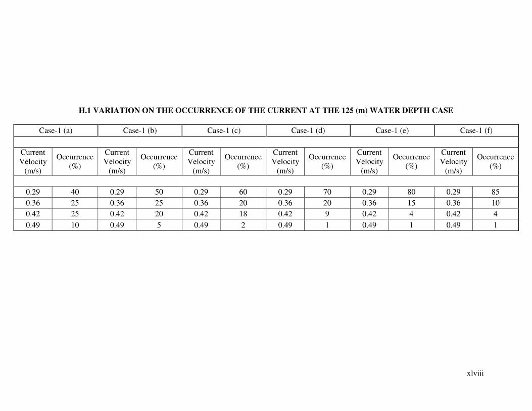
xlviii
H.1 VARIATION ON THE OCCURRENCE OF THE CURRENT AT THE 125 (m) WATER DEPTH CASE
Case-1 (a) Case-1 (b) Case-1 (c) Case-1 (d) Case-1 (e) Case-1 (f)
Current
Velocity
(m/s)
Occurrence
(%)
Current
Velocity
(m/s)
Occurrence
(%)
Current
Velocity
(m/s)
Occurrence
(%)
Current
Velocity
(m/s)
Occurrence
(%)
Current
Velocity
(m/s)
Occurrence
(%)
Current
Velocity
(m/s)
Occurrence
(%)
0.29 40 0.29 50 0.29 60 0.29 70 0.29 80 0.29 85
0.36 25 0.36 25 0.36 20 0.36 20 0.36 15 0.36 10
0.42 25 0.42 20 0.42 18 0.42 9 0.42 4 0.42 4
0.49 10 0.49 5 0.49 2 0.49 1 0.49 1 0.49 1
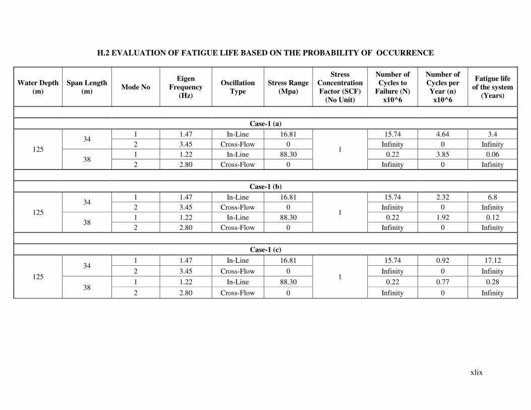
xlix
H.2 EVALUATION OF FATIGUE LIFE BASED ON THE PROBABILITY OF OCCURRENCE
Water Depth
(m)
Span Length
(m) Mode No
Eigen
Frequency
(Hz)
Oscillation
Type
Stress Range
(Mpa)
Stress
Concentration
Factor (SCF)
(No Unit)
Number of
Cycles to
Failure (N)
x10^6
Number of
Cycles per
Year (n)
x10^6
Fatigue life
of the system
(Years)
Case-1 (a)
125
34 1 1.47 In-Line 16.81
1
15.74 4.64 3.4
2 3.45 Cross-Flow 0 Infinity 0 Infinity
38 1 1.22 In-Line 88.30 0.22 3.85 0.06
2 2.80 Cross-Flow 0 Infinity 0 Infinity
Case-1 (b)
125
34 1 1.47 In-Line 16.81
1
15.74 2.32 6.8
2 3.45 Cross-Flow 0 Infinity 0 Infinity
38 1 1.22 In-Line 88.30 0.22 1.92 0.12
2 2.80 Cross-Flow 0 Infinity 0 Infinity
Case-1 (c)
125
34 1 1.47 In-Line 16.81
1
15.74 0.92 17.12
2 3.45 Cross-Flow 0 Infinity 0 Infinity
38 1 1.22 In-Line 88.30 0.22 0.77 0.28
2 2.80 Cross-Flow 0 Infinity 0 Infinity
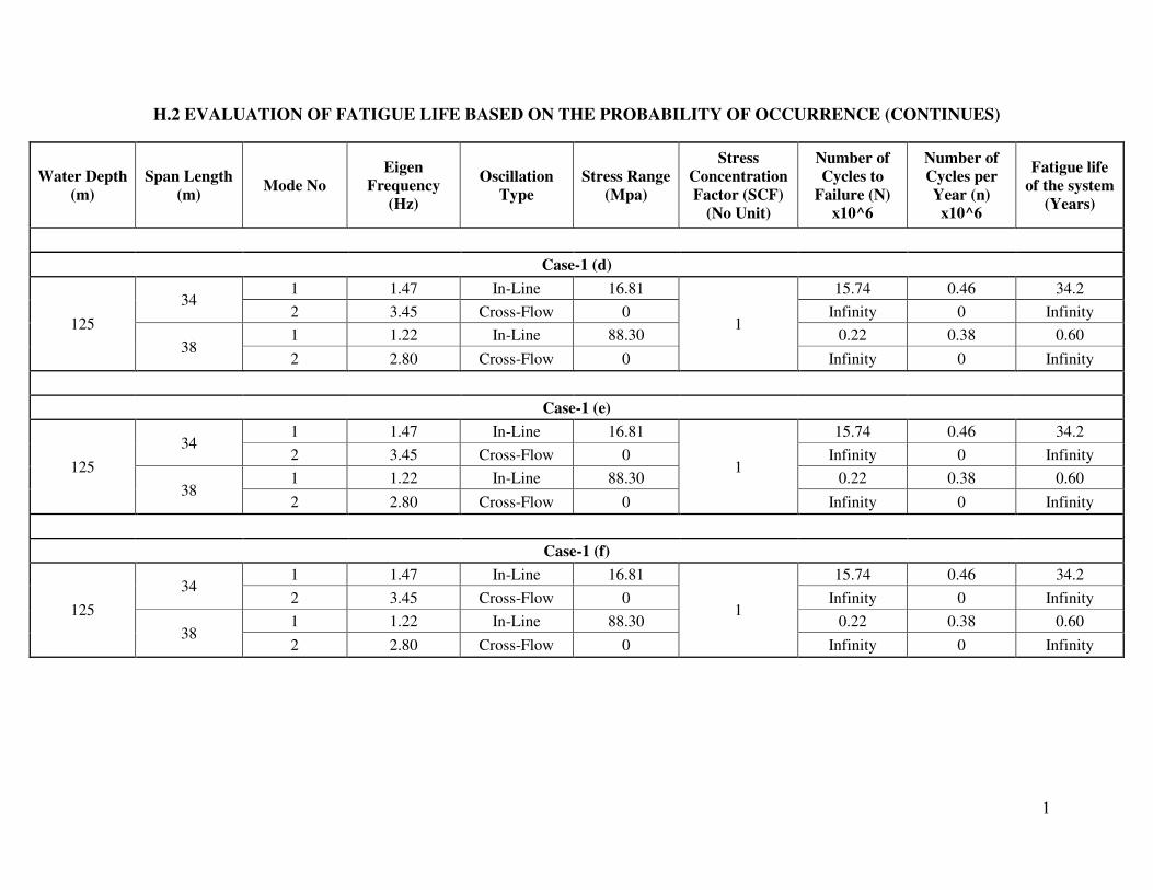
l
H.2 EVALUATION OF FATIGUE LIFE BASED ON THE PROBABILITY OF OCCURRENCE (CONTINUES)
Water Depth
(m)
Span Length
(m) Mode No
Eigen
Frequency
(Hz)
Oscillation
Type
Stress Range
(Mpa)
Stress
Concentration
Factor (SCF)
(No Unit)
Number of
Cycles to
Failure (N)
x10^6
Number of
Cycles per
Year (n)
x10^6
Fatigue life
of the system
(Years)
Case-1 (d)
125
34 1 1.47 In-Line 16.81
1
15.74 0.46 34.2
2 3.45 Cross-Flow 0 Infinity 0 Infinity
38 1 1.22 In-Line 88.30 0.22 0.38 0.60
2 2.80 Cross-Flow 0 Infinity 0 Infinity
Case-1 (e)
125
34 1 1.47 In-Line 16.81
1
15.74 0.46 34.2
2 3.45 Cross-Flow 0 Infinity 0 Infinity
38 1 1.22 In-Line 88.30 0.22 0.38 0.60
2 2.80 Cross-Flow 0 Infinity 0 Infinity
Case-1 (f)
125
34 1 1.47 In-Line 16.81
1
15.74 0.46 34.2
2 3.45 Cross-Flow 0 Infinity 0 Infinity
38 1 1.22 In-Line 88.30 0.22 0.38 0.60
2 2.80 Cross-Flow 0 Infinity 0 Infinity