Embed Size (px)
Citation preview
UNIVERSITA CATTOLICA DEL SACRO CUORESEDE DI BRESCIA
Facolta di Scienze Matematiche, Fisiche e Naturali
Corso di Laurea in Fisica
Tesi di Laurea Magistrale
Dynamics of the Symmetry Breakingin Ordered Phases
Relatore:Ch.mo Prof. Claudio GiannettiCorrelatore:Ch.mo Prof. Francesco Banfi
Candidato:Marco GandolfiMatricola n. 4108849
Anno Accademico 2013/2014
15 dicembre 2014

Contents
1 Model 121.1 The Ginzburg-Landau Theory . . . . . . . . . . . . . . . . . . . . . 121.2 Equation for a spatially inhomogeneous time-independent order pa-
rameter . . . . . . . . . . . . . . . . . . . . . . . . . . . . . . . . . 171.3 Ginzburg-Landau equation for a spatially inhomogeneous time-dependent
order parameter . . . . . . . . . . . . . . . . . . . . . . . . . . . . . 211.4 Linearized Ginzburg-Landau equation for a spatially inhomogeneous
time-dependent order parameter . . . . . . . . . . . . . . . . . . . . 23
2 COMSOL Multiphysics main features 25
3 Dynamics of the order parameter in the homogeneous case 293.1 Time-independent equilibrium order parameter with no damping . . 29
3.1.1 Results . . . . . . . . . . . . . . . . . . . . . . . . . . . . . . 293.1.2 Technical details . . . . . . . . . . . . . . . . . . . . . . . . 37
3.2 Time-independent equilibrium order parameter with damping . . . 383.2.1 Results . . . . . . . . . . . . . . . . . . . . . . . . . . . . . . 383.2.2 Technical details . . . . . . . . . . . . . . . . . . . . . . . . 44
3.3 Time-dependent equilibrium order parameter with no damping . . . 453.3.1 Results . . . . . . . . . . . . . . . . . . . . . . . . . . . . . . 453.3.2 Technical details . . . . . . . . . . . . . . . . . . . . . . . . 49
4 Reflectivity for a system in overdamped regime 504.1 Results . . . . . . . . . . . . . . . . . . . . . . . . . . . . . . . . . . 54
4.1.1 Homogeneous excitation . . . . . . . . . . . . . . . . . . . . 544.1.2 Quasi-homogeneous excitation . . . . . . . . . . . . . . . . . 634.1.3 Strongly inhomogeneous excitation . . . . . . . . . . . . . . 674.1.4 Bulk system . . . . . . . . . . . . . . . . . . . . . . . . . . . 714.1.5 Comparison of the analyzed cases . . . . . . . . . . . . . . . 754.1.6 Bulk system: comparison between simulations and experi-
mental data . . . . . . . . . . . . . . . . . . . . . . . . . . . 77
3
4.2 Technical details . . . . . . . . . . . . . . . . . . . . . . . . . . . . 85
5 Super-lattice composed by materials with broken symmetry 915.1 Many unit cells geometry . . . . . . . . . . . . . . . . . . . . . . . . 935.2 One unit cell geometry . . . . . . . . . . . . . . . . . . . . . . . . . 97
4
Introduction
When a second order phase transition occurs you can introduce an order parame-ter η, obeying to the well-known Ginzburg-Landau equation.
This equation is very general, because it applies for any second order phase tran-sition. There are a lot of applications, such as the study evolution of the orderparameter in superconductors or the analyze of the Higgs modes. There is animportant link between the superconductivity and the Higgs mechanism: in bothcases there is a symmetry breaking.
In particular, as we will see in chapter 1, the free energy for a superconductorassumes the “Mexican hat” shape, with a degenerate circle of minima (the groundstate), defined by the order parameter η = Aeiϕ, (see figure 1).In Quantum Field Theory there is an analogy because the Lagrangian can bewritten as a function of the field η:
L = ∂µη∂µη − V (η),
where the potential V (η) has the “Mexican hat” shape:
5
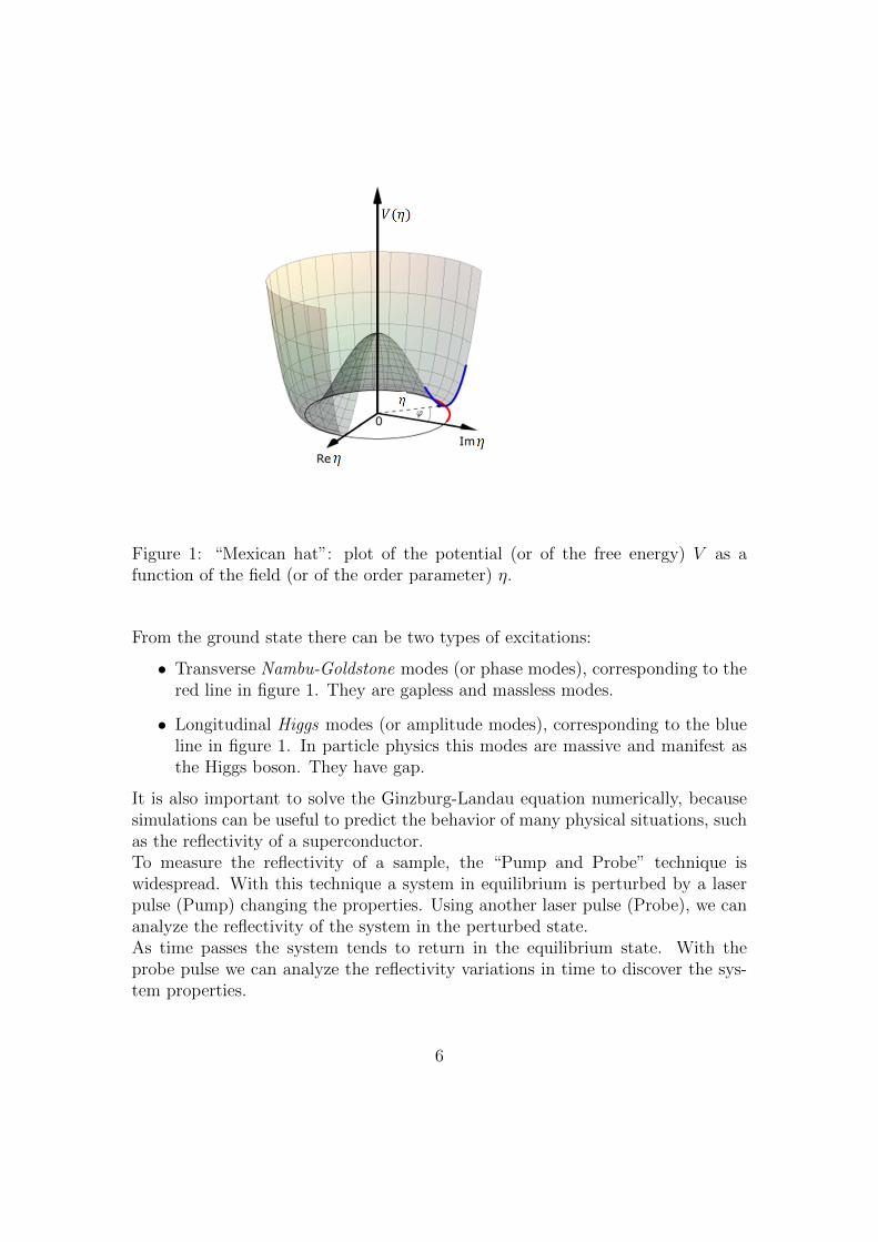
Figure 1: “Mexican hat”: plot of the potential (or of the free energy) V as afunction of the field (or of the order parameter) η.
From the ground state there can be two types of excitations:
• Transverse Nambu-Goldstone modes (or phase modes), corresponding to thered line in figure 1. They are gapless and massless modes.
• Longitudinal Higgs modes (or amplitude modes), corresponding to the blueline in figure 1. In particle physics this modes are massive and manifest asthe Higgs boson. They have gap.
It is also important to solve the Ginzburg-Landau equation numerically, becausesimulations can be useful to predict the behavior of many physical situations, suchas the reflectivity of a superconductor.To measure the reflectivity of a sample, the “Pump and Probe” technique iswidespread. With this technique a system in equilibrium is perturbed by a laserpulse (Pump) changing the properties. Using another laser pulse (Probe), we cananalyze the reflectivity of the system in the perturbed state.As time passes the system tends to return in the equilibrium state. With theprobe pulse we can analyze the reflectivity variations in time to discover the sys-tem properties.
6
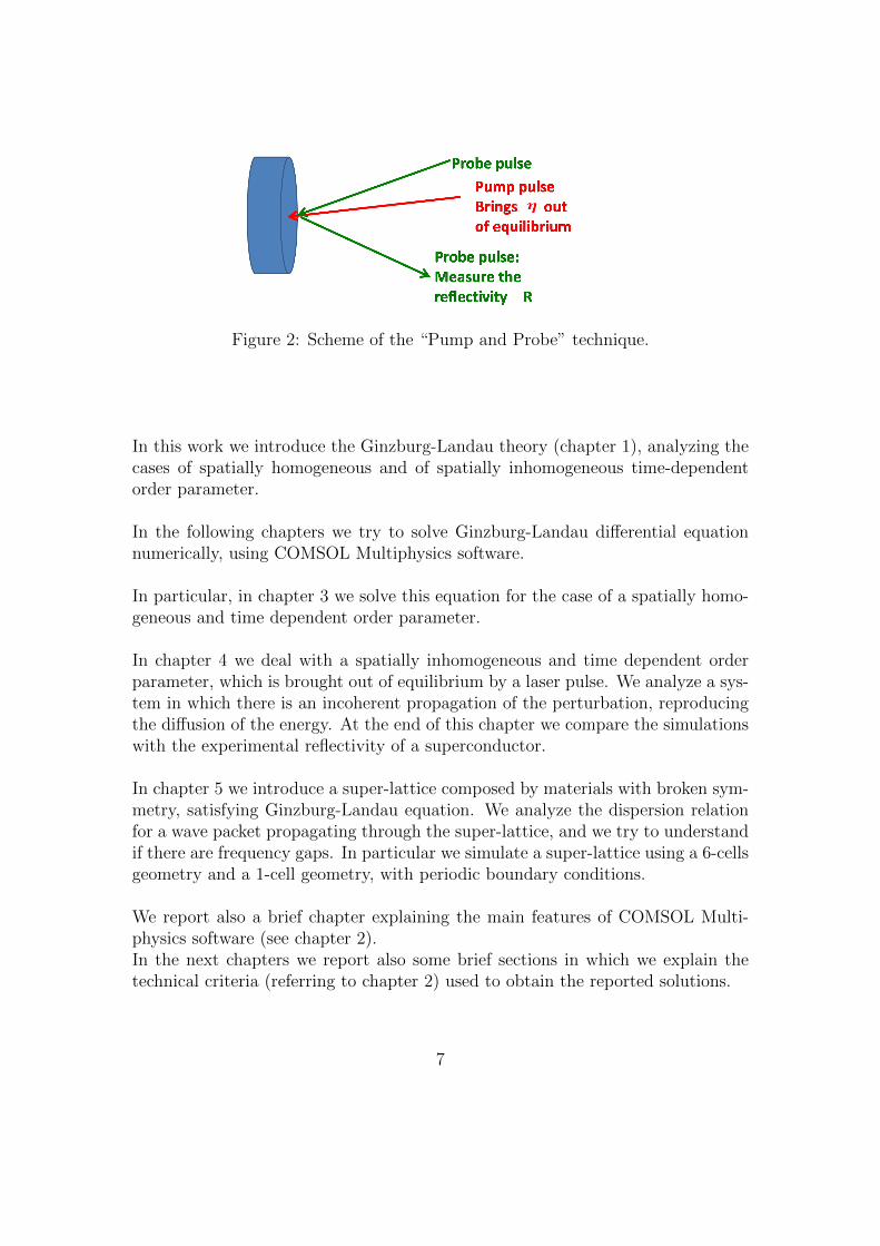
Figure 2: Scheme of the “Pump and Probe” technique.
In this work we introduce the Ginzburg-Landau theory (chapter 1), analyzing thecases of spatially homogeneous and of spatially inhomogeneous time-dependentorder parameter.
In the following chapters we try to solve Ginzburg-Landau differential equationnumerically, using COMSOL Multiphysics software.
In particular, in chapter 3 we solve this equation for the case of a spatially homo-geneous and time dependent order parameter.
In chapter 4 we deal with a spatially inhomogeneous and time dependent orderparameter, which is brought out of equilibrium by a laser pulse. We analyze a sys-tem in which there is an incoherent propagation of the perturbation, reproducingthe diffusion of the energy. At the end of this chapter we compare the simulationswith the experimental reflectivity of a superconductor.
In chapter 5 we introduce a super-lattice composed by materials with broken sym-metry, satisfying Ginzburg-Landau equation. We analyze the dispersion relationfor a wave packet propagating through the super-lattice, and we try to understandif there are frequency gaps. In particular we simulate a super-lattice using a 6-cellsgeometry and a 1-cell geometry, with periodic boundary conditions.
We report also a brief chapter explaining the main features of COMSOL Multi-physics software (see chapter 2).In the next chapters we report also some brief sections in which we explain thetechnical criteria (referring to chapter 2) used to obtain the reported solutions.
7
References
1. Daniel Sherman, Uwe S. Pracht, Boris Gorshunov, Shachaf Poran, JohnJesudasan, Madhavi Chand, Pratap Raychaudhuri, Mason Swanson, NandiniTrivedi, Assa Auerbach, Marc Scheffler, Aviad Frydman, Martin Dressel,The Higgs Mode in Disordered Superconductors Close to a Quantum PhaseTransition.
2. Ryusuke Matsunaga, Yuki I. Hamada, Kazumasa Makise, Yoshinori Uzawa,Hirotaka Terai, Zhen Wang, Ryo Shimano, Higgs Amplitude Mode in the BCSSuperconductors Nb1−xTixN induced by Terahertz Pulse Excitation, PhysicalReview Letters, 2013.
3. Ryusuke Matsunaga, Naoto Tsuji, Hiroyuki Fujita, Arata Sugioka, Kazu-masa Makise, Yoshinori Uzawa, Hirotaka Terai, Zhen Wang, Hideo Aoki,Ryo Shimano,Light-induced collective pseudospin precession resonating withHiggs mode in a superconductor, Siencexpress.
4. M.-A. Measson, Y. Gallais, M. Cazayous, B. Clair, P. Rodiere, L. Cario, A.Sacuto,Amplitude ‘Higgs’ mode in 2H −NbSe2 Superconductor.
5. Yafis Barlas, C. M. Varma,Amplitude or Higgs modes in d-wave supercon-ductors, PHYSICAL REVIEW (2013).
6. T. Cea and L. Benfatto, On the nature of the Higgs (amplitude) mode in thecoexisting superconducting and charge-density-wave state, (2014).
8


Dynamics of the Symmetry Breaking
in Ordered Phases

Chapter 1
Model
In this chapter we introduce the Ginzburg-Landau theory for a second orderphase transition.
1.1 The Ginzburg-Landau Theory
A physical system experiences a “phase transition” when it changes from onestate to another with different properties.
Usually a phase transition occurs when some parameters, such as the temperature,the applied magnetic field, the concentration of charge carriers, the pressure, ... ,change and cross a critical value. Phase transitions can be classified in:
• First order phase transitions, characterized by the following features:
– The energy1 of the system has a discontinuity at the critical point.
– Spatial coexistence of different phases at the critical point.
– Hysteresis.
An example of first order phase transition is when a solid melts. In this casethe control parameter is the temperature of the system.
1In this case we mean the internal energy U , satisfying the relation dU = TdS−PdV +µdN ,where T is the temperature, S the entropy, P the pressure, V the volume, µ the chemical potentialand N the number of particles of the system.
12
• Second order phase transitions, characterized by the following features:
– The energy of the system is continuous at the critical point but its firstderivative (the specific heat CV ) is not continuous.
– When the phase transition occurs the system looses symmetry.
– There is an “order parameter”, which is a scalar or a vector quantityequal to 0 when the system is in the state with higher symmetry, anddifferent from 0 when the system is in the state with lower symmetry.
– When the system is in the state with lower symmetry and moves towardthe critical point, the order parameter tends to go to 0 with continuity.At the critical point the order parameter is 0 and the system is in thestate with higher symmetry. So in an homogeneous system there cannotbe spatial coexistence of different phases at equilibrium.
Examples of second order phase transitions are the transition from ferromag-netic to paramagnetic materials and the transition from a superconductingstate to a normal state. In both these cases the control parameter is the tem-perature of the system. When the temperature falls under a critical valueTc, the system looses symmetry.
In this work we focus our attention on second order phase transitions only.
As mentioned before, the order parameters can be scalars (real or complex), orvectors. In this work we analyze the case in which the order parameter is a scalar.
In the following we will use the following notation: T for the temperature and Pthe pressure of the system; η for the order parameter; Ω(P, T, ...) for the dimen-sionless free energy (i.e. the free energy divided by a constant energy), expressedas a function of the pressure, of the temperature or of the other control parameters.
We assume that Ω is a function of η and then we can make an expansion:
Ω(P, T, η) = Ω0(P, T ) + c1η + α2(P, T ) |η|2 + c3 |η|2 η +1
2β4(P, T ) |η|4 + ... (1.1)
Since the free energy is a real number, the coefficient α2 and β4 are real.
Let’s assume to work with a dimensionless order parameter.If the order parameter is small we can cut this expansion to the 4th power.
13

Next we assume that the system is invariant for the transformation η → −η, i.e.the +η or −η values must give the same configuration. As a consequence, theexpansion of the free energy must contain terms with only even powers of η.
If we suppose that the coefficient β4 does not depend on the temperature we obtainthe following expression:
Ω(P, T, η) = Ω0(P, T ) + α2(P, T ) |η|2 +1
2β4(P ) |η|4 (1.2)
The equilibrium state is obtained when the free energy is minimum. If β4 < 0,the free energy from expression (1.2) would continuously decrease for large valuesof the order parameter; this is in contrast to the assumption that the expansioncan be stopped at the 4th power (which implies a small η). Therefore we assumeβ4 > 0.
Now we can evaluate the minimum of the free energy, using:
∂Ω
∂η∗= 0.
Reminding that |η|2 = ηη∗, we obtain:
α2(P, T )η + β4(P ) |η|2 η = 0, (1.3)
which gives the following solutions:
η = 0, (1.4)
|η| =√−α2
β4. (1.5)
If α2 > 0, only solution (1.4) represents the minimum (the other solution is imagi-nary, therefore it has no physical meaning); if α2 < 0, the solution (1.5) representsthe minimum (the other solution represents a local maximum, as we can see fromthe following graph).
14

Figure 1.1: Plot of the free energy as a function of the order parameter amplitude.The continuous line describes a case in which α2 < 0; the dashed line describes acase in which α2 > 0.
If α2 > 0 the order parameter at equilibrium is 0, if α2 < 0 the order parameterat equilibrium is
√−α2/β4.
15

As a consequence, it is natural to assume that a phase transition occurs when α2
changes sign. If the phase transition occurs when the system reaches a criticaltemperature Tc, we can assume that:
α2(P, T ) = a(P ) (T − Tc) , (1.6)
and a(P ) is a real positive number. Consequently the order parameter at equilib-rium is:
|ηeq| =
0 if T ≥ Tc√
− a(P )
β4(P )(T − Tc) if T < Tc.
(1.7)
16

1.2 Equation for a spatially inhomogeneous
time-independent order parameter
In this section we deal the case of a spatially inhomogeneous, but time-independent, order parameter analyzing the equilibrium situation.
If the system is characterized by a space-dependent order parameter, the expressionof the free energy for a small order parameter becomes:
Ω(P, T, η) =
∫V
[ω0(P, T ) + A(P, T ) |η|2 +
1
2B(P ) |η|4 + λ |∇η|2
]dV, (1.8)
where the last term has been introduced to consider the free energy correctionsdue to a spatially inhomogeneous order parameter.The parameter λ is called “stiffness”. If the order parameter is brought out ofequilibrium in a certain spatial point,
√λ describes the spatial scale at which the
order parameter has restored to his equilibrium value.
Now we need to calculate the functional derivative of the free energy with respectto η∗. So we make the substitution η → η + δη to obtain:
δΩ(P, T, η) =
∫V
[ω0(P, T ) + A(P, T ) (η + δη) (η∗ + δη∗) +
+1
2B(P ) (η + δη)2 (η∗ + δη∗)2 +
+ λ∇ (η + δη) · ∇ (η∗ + δη∗)] dV − Ω(P, T, η) =
=
∫V
[ω0(P, T ) + A(P, T ) |η|2 + A(P, T )ηδη∗ + A(P, T )η∗δη
+1
2B(P ) |η|4 +B(P )δη |η|2 η∗ +B(P )δη∗ |η|2 η +O
((δη)2
)+
+λ |∇η|2 + λ∇η · ∇δη∗ + λ∇η∗ · ∇δη + λ |∇δη|2]dV − Ω(P, T, η).
In evaluating the functional derivative of the free energy with respect to η∗ wenote that:
• All the terms not explicitly containing δη∗ cancel out.
17
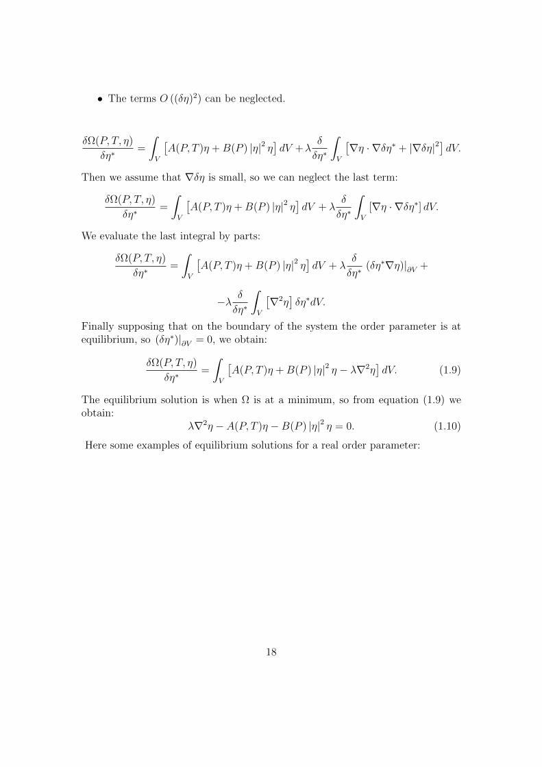
• The terms O ((δη)2) can be neglected.
δΩ(P, T, η)
δη∗=
∫V
[A(P, T )η +B(P ) |η|2 η
]dV +λ
δ
δη∗
∫V
[∇η · ∇δη∗ + |∇δη|2
]dV.
Then we assume that ∇δη is small, so we can neglect the last term:
δΩ(P, T, η)
δη∗=
∫V
[A(P, T )η +B(P ) |η|2 η
]dV + λ
δ
δη∗
∫V
[∇η · ∇δη∗] dV.
We evaluate the last integral by parts:
δΩ(P, T, η)
δη∗=
∫V
[A(P, T )η +B(P ) |η|2 η
]dV + λ
δ
δη∗(δη∗∇η)|∂V +
−λ δ
δη∗
∫V
[∇2η
]δη∗dV.
Finally supposing that on the boundary of the system the order parameter is atequilibrium, so (δη∗)|∂V = 0, we obtain:
δΩ(P, T, η)
δη∗=
∫V
[A(P, T )η +B(P ) |η|2 η − λ∇2η
]dV. (1.9)
The equilibrium solution is when Ω is at a minimum, so from equation (1.9) weobtain:
λ∇2η − A(P, T )η −B(P ) |η|2 η = 0. (1.10)
Here some examples of equilibrium solutions for a real order parameter:
18
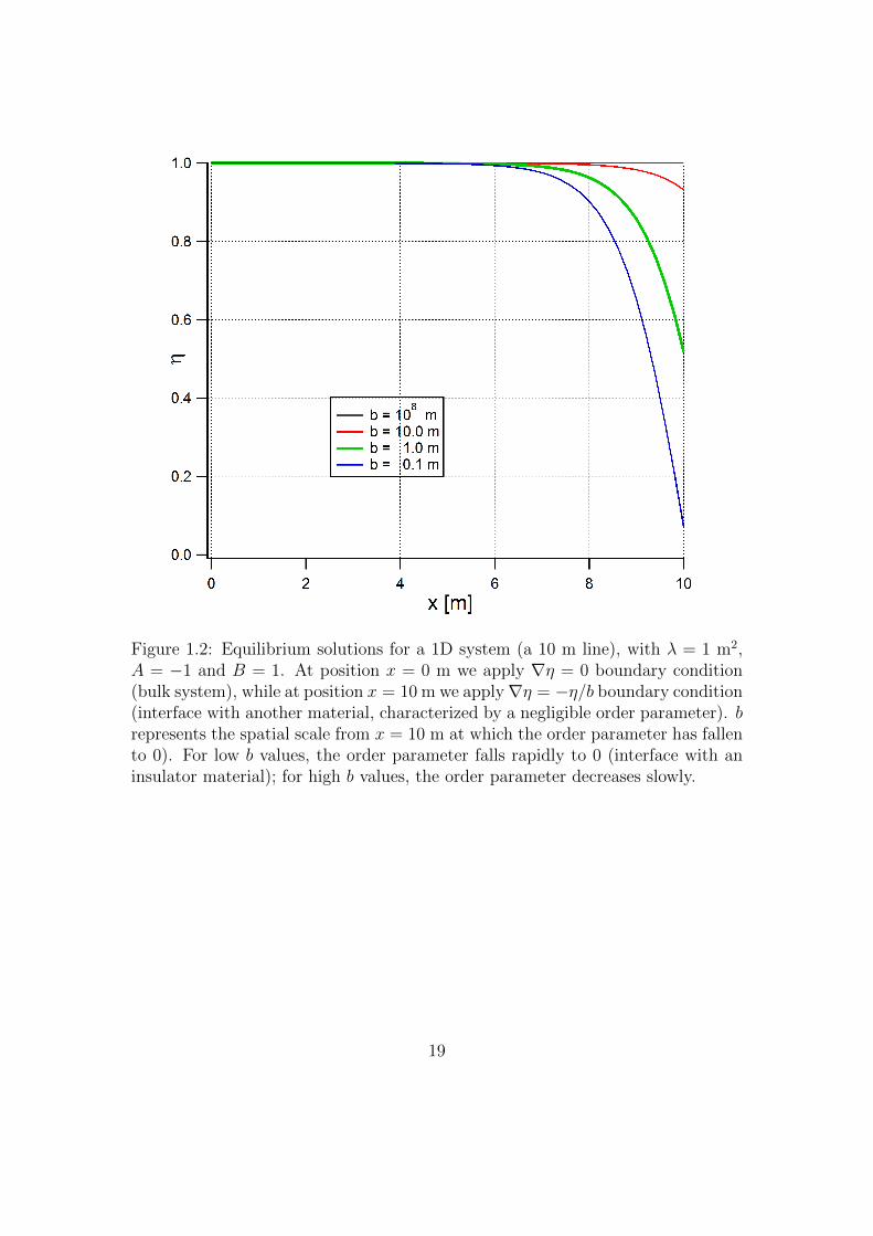
Figure 1.2: Equilibrium solutions for a 1D system (a 10 m line), with λ = 1 m2,A = −1 and B = 1. At position x = 0 m we apply ∇η = 0 boundary condition(bulk system), while at position x = 10 m we apply∇η = −η/b boundary condition(interface with another material, characterized by a negligible order parameter). brepresents the spatial scale from x = 10 m at which the order parameter has fallento 0). For low b values, the order parameter falls rapidly to 0 (interface with aninsulator material); for high b values, the order parameter decreases slowly.
19

Figure 1.3: Equilibrium solution (color scale) for a 2D system (a 20 m × 10 mrectangle), with λ = 1 m2, A = −1 and B = 1. At vertical sides and lowerhorizontal side we apply ∇η = 0 boundary condition (bulk system),while at upperhorizontal side we apply ∇η = −η/b boundary condition (interface with anothermaterial, characterized by b = 1 m).
20
1.3 Ginzburg-Landau equation for a spatially in-
homogeneous time-dependent order param-
eter
In this section we deal the case of a spatially inhomogeneous and time-dependentorder parameter.
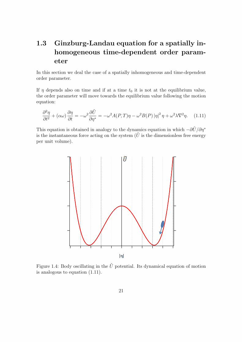
If η depends also on time and if at a time t0 it is not at the equilibrium value,the order parameter will move towards the equilibrium value following the motionequation:
∂2η
∂t2+ (αω)
∂η
∂t= −ω2 ∂U
∂η∗= −ω2A(P, T )η − ω2B(P ) |η|2 η + ω2λ∇2η. (1.11)
This equation is obtained in analogy to the dynamics equation in which −∂U/∂η∗is the instantaneous force acting on the system (U is the dimensionless free energyper unit volume).
Figure 1.4: Body oscillating in the U potential. Its dynamical equation of motionis analogous to equation (1.11).
21
In equation (1.11), ω has been introduced to safeguard the dimensions in theequation and is related to the “frequency of oscillation” of η around its equilibriumvalue.α is a coefficient representing the “damping” of η.In the limit αω >> 1 relation (1.11) reduces to the original Ginzburg-LandauKinetic Equation:
(αω)∂η
∂t= −ω2A(P, T )η − ω2B(P ) |η|2 η + ω2λ∇2η, (1.12)
describing a system in which the order parameter does not make oscillations.This is a diffusion-like equation, describing an incoherent propagation of the orderparameter.
However, since equation (1.11) is more general than equation (1.12), we will dealonly with equation (1.11), which is called Ginzburg-Landau (GL) equation.
If the order parameter is real, equation (1.11) reduces to:
∂2η
∂t2+ (αω)
∂η
∂t+ ω2A(P, T )η + ω2B(P )η3 − ω2λ∇2η = 0.
This equation has the form of a wave equation in which ω2Aη + ω2Bη3 is thesource.Last equation can be rewritten as:
1
ω2
∂2η
∂t2+(αω
) ∂η∂t
+ A(P, T )η +B(P )η3 − λ∇2η = 0. (1.13)
22
1.4 Linearized Ginzburg-Landau equation for a
spatially inhomogeneous time-dependent or-
der parameter
Equation (1.13) contains a cubic term, increasing the difficulties to obtain asolution. Therefore if the order parameter differs from the equilibrium solutionslightly we can approximate the cubic term with a linear term in order to obtaina easier to handle equation. In this section we describe the approximation processto linearize equation (1.13).
We suppose that ηeq(x) is the equilibrium solution of equation (1.13), i.e. ηeq(x)satisfies relation (1.10) for a real order parameter. Evidently ηeq(x) does notdepend on time.
Defining the displacement of the order parameter with respect to the equilibriumvalue as:
δη(x, t) = η(x, t)− ηeq(x), (1.14)
we can make the substitution η(x, t) → ηeq(x) + δη(x, t) in equation (1.13) toobtain:
1
ω2
∂2δη
∂t2+(αω
) ∂δη∂t
+ A(P, T )δη + 3B(P )η2eqδη +O((δη)2
)− λ∇2δη =
= λ∇2ηeq − A(P, T )ηeq −B(P )η3eq. (1.15)
Reminding that ηeq(x) satisfies relation (1.10) for a real order parameter, we candeduce that the right-hand side of equation (1.15) is 0.
Further, if the order parameter is slightly different from the equilibrium value,so that the terms O
((δη)2
)can be neglected, we can derive the Linearized
Ginzburg-Landau equation for a real order parameter:
1
ω2
∂2δη
∂t2+(αω
) ∂δη∂t
+[A(P, T ) + 3B(P )η2eq
]δη − λ∇2δη = 0. (1.16)
23

References
1. Michael Tinkham, Introduction to Superconductivity, McGraw-Hill, Inc.
2. Anthony James Leggett, Quantum Liquids. Bose condensation and Cooperpairing in condensed-matter systems, Oxford Graduate Texts, 2006.
24

Chapter 2
COMSOL Multiphysics mainfeatures
In this chapter we explain briefly the main properties of the used program.
COMSOL Multiphysics is a software for solving differential equations comingfrom physical problems. Since this work deals with the numerical solutions ofthe GL equation obtained using the COMSOL Multiphysics software, this briefchapter explains the main features of this program.
As we start the program, a “Model Wizard” procedure allows the user to choosethe dimensions of the model:
• “0D”, if the space is not involved in the model.
• “1D”. The spatial coordinate is indicated with x.
• “1D-Axisymmetric”, if the model is in 2 dimensions, but there is a rotationalsymmetry along the angle ϕ, so the model involves 1 space variable only, theradial coordinate r.
• “2D”. The spatial coordinates are indicated with (x, y).
• “2D-Axisymmetric”, if the model is in 3 dimensions, but there is a rotationalsymmetry along the angle ϕ, so the model involves 2 space variables only,the radial coordinate r and the height coordinate z.
• “3D”. The spatial coordinates are indicated with (x, y, z).
Then we will be asked to add a “physics”. Since we need to solve a differentialequation, in this work we use:
25

• “Global ODEs and DAEs” in Chapter 3.
• “Coefficient Form PDE” in all the other Chapters. This type of physics isnot available for a “0D” model.
Finally we will be asked to choose the “Study Type”. In particular in this workwe use:
• “Stationary Study”, if we are interested in an equilibrium solution, in thecase of a time-dependent model.
• “Time Dependent Study”, if we are interested in a solution at different times.
• “Eigenvalue Study”, if we are interested in the eigenvalues of an equation.
Then the “Model Wizard” procedure stops and we can modify the model addingitems. To do this we can right-click on each voice in the “Model Builder” space.In particular we can add global “parameters” of the model right-clicking on“Global Definitions”.We can also use a previous solution as an input function of the model. To do this,under the voice with the name of the model, we can add a interpolation function.If we have not a “0D” model, the voice “Geometry” appears and we can choosethe shape of the spatial domains.
Under the voice with the name of the model there is the voice concerning the usedphysics. In this work we use the following 2 possibilities:
• “Global ODEs and DAEs”, used in Chapter 3, for a “0D” model. Under thevoice “Global ODEs and DAEs” there is a voice concerning the equation.The equation is written as:
f(u, ut, utt) = 0,
where u is the solution, while ut and utt are the first and the second derivateof u with respect to time.Here we are allowed to type the expression of f(u, ut, utt) and the initialvalues of ut and utt.
• “Coefficient Form PDE” in all the other Chapters. This type of physics isnot available for a “0D” model. Under the voice “Global ODEs and DAEs”we are asked the dimensions of the dependent variable u and of the “Sourceterm” f in the equation; then there is a voice concerning the equation. Theequation is written as:
ea∂2u
∂t2+ da
∂u
∂t+∇ · (−c∇u−αu+ γ) + β · ∇u+ au = f, (2.1)
26
and we can choose the value of the scalar coefficients ea, da, a, of the vectorcoefficients α, β, γ and of the matrix coefficient c. These coefficients canbe a function on the spatial coordinates. As for the source term f , we areasked to introduce a more general expression, which can be a function of thedependent variable u and of space coordinates.If we choose an “Eigenvalue Study”, COMSOL Multiphysics makes a tem-poral Fourier transformation on the dependent variable u; so each derivatewith respect to time is substituted by the eigenvalue λ to obtain:
λ2eau2 − λdau+∇ · (−c∇u−αu+ γ) + β · ∇u+ au = f.
To solve a “Coefficient Form PDE” it is necessary to assign boundary con-ditions on all the boundaries of the geometry, holding for all times. Inparticular we use:
– “Zero Flux” boundary condition:
−n · (−c∇u−αu+ γ) = 0,
where n is the external normal to the boundary.
– “Dirichlet” boundary condition, if the dependent variable is constrainedto be a specified value on the boundary.
– “Flux/Source” boundary condition:
−n · (−c∇u−αu+ γ) = g − qu,
where n is the external normal to the boundary.
To solve a “Coefficient Form PDE” it is necessary to assign also the initialvalue of the dependent variable u (and its first derivative with respect totime) on all the domains. To do this we can type the desired expressionunder the “Initial Values” voice.In the case of “Time Dependent Study”, the “Initial Values” expression isthe solution at the initial time.In the case of “Stationary Study” and of “Eigenvalue Study”, the “InitialValues” expression represents an initial guess for the solver. For a wellconstrained problem, the particular expression assigned as “Initial Values”should not influence the final solution.
COMSOL Multiphysics solves the differential equation using the Finite ElementsMethod. The initial problem to solve is approximated with another problem whichhas a finite number of unknown parameters.
27
So the times range and the space domains at which we have to calculate a solutionare discretized and the software solves the differential equation at some pointsonly. We can choose the number of discretization points, increasing them to makethe solution more precise (but the computational costs increase). Finally, whenthe software has obtained the solution in all the discretization points, it will makean interpolation to give the solution in all the requested domains and times.
If the model has a geometry (not the 0D), the set of spatial discretization pointsis called “Mesh”. Acting in “Mesh” voice we can choose the distance and thespatial collocation of the discretization points.
For all the specified physics there is a “Study” node, specifying the algorithms andthe parameters used to obtain a solution. In particular for this work, sometimesit is necessary to modify the following voices:
• For a “Stationary Study” it is sometimes necessary to diminish “Relativetolerance” to obtain a more precise solution. Sometimes the number of it-eration is not enough to reach a solution satisfying the value of “Relativetolerance”; therefore it could be necessary to increase the “Maximum num-ber of iterations”.
• For a “Time Dependent Study” it is necessary to open the voice “Time-Dependent Solver” under the study node and to choose the “Generalizedalpha” Method, instead of the “BDF” Method (which generates numericalerrors in the case we are dealing with). Then to improve the precision of thesolution we have to set “Manual” at the voice “Steps taken by solver” andthan choose an opportune “Time step”. COMSOL Multiphysics solves thedifferential equation in a discrete number of temporal points. The temporaldistance among these points is specified by the “Time step” voice. Onceobtained the solution in these points, COMSOL Multiphysics makes an in-terpolation to give the solution for the times listed under the voice “Step 1:Time Dependent”.
• For an “Eigenvalue Study” we are asked to choose the “Desired number ofeigenvalues” and where to search the eigenvalues around. If we choose tosearch an high number of eigenvalues, we may need to increase the “Maxi-mum number of eigenvalue iterations”, under the voice “Eigenvalue Solver1”.
Right clicking on “Study” node we can activate a “Parametric Sweep”, i.e. welet vary certain parameters over a specified range and for each value of theparameters the software evaluates a solution.
28
Chapter 3
Dynamics of the order parameterin the homogeneous case
In this chapter we discuss the solutions of GL equation in the case of a spatiallyhomogeneous order parameter.
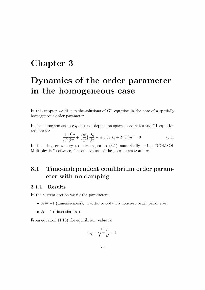
In the homogeneous case η does not depend on space coordinates and GL equationreduces to:
1
ω2
∂2η
∂t2+(αω
) ∂η∂t
+ A(P, T )η +B(P )η3 = 0. (3.1)
In this chapter we try to solve equation (3.1) numerically, using “COMSOLMultiphysics” software, for some values of the parameters ω and α.
3.1 Time-independent equilibrium order param-
eter with no damping
3.1.1 Results
In the current section we fix the parameters:
• A ≡ −1 (dimensionless), in order to obtain a non-zero order parameter;
• B ≡ 1 (dimensionless).
From equation (1.10) the equilibrium value is:
ηeq =
√−AB
= 1.
29
In this section we fix our attention on the case of a system without damping(α = 0).
• For any value of ω and α, if we choose η|t=0 = 1 and dηdt
∣∣t=0
= 0 s−1 as initialconditions, the solution is
η(t) = ηeq = 1, ∀t > 0
since the system is in a stable equilibrium position, so it does not move.
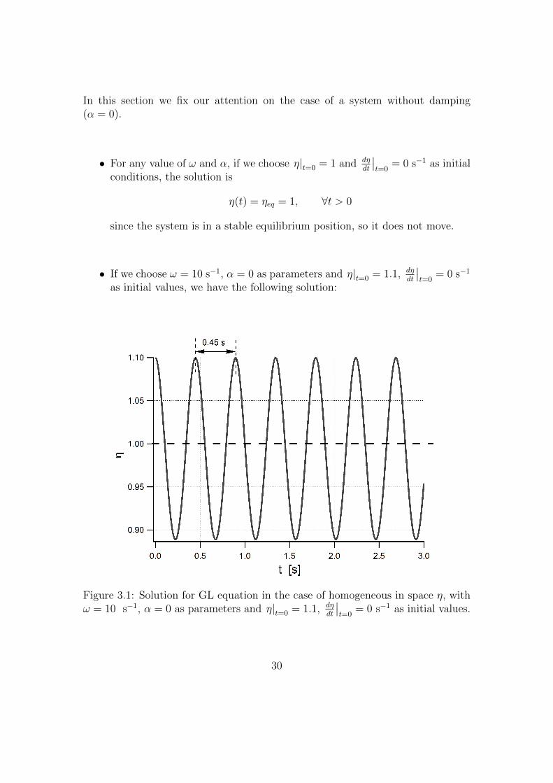
• If we choose ω = 10 s−1, α = 0 as parameters and η|t=0 = 1.1, dηdt
∣∣t=0
= 0 s−1
as initial values, we have the following solution:
Figure 3.1: Solution for GL equation in the case of homogeneous in space η, withω = 10 s−1, α = 0 as parameters and η|t=0 = 1.1, dη
dt
∣∣t=0
= 0 s−1 as initial values.
30
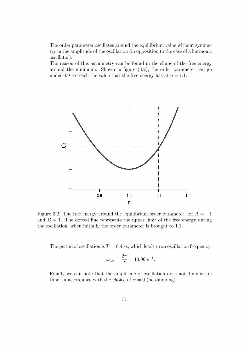
The order parameter oscillates around the equilibrium value without symme-try in the amplitude of the oscillation (in opposition to the case of a harmonicoscillator).The reason of this asymmetry can be found in the shape of the free energyaround the minimum. Shown in figure (3.2), the order parameter can gounder 0.9 to reach the value that the free energy has at η = 1.1.
Figure 3.2: The free energy around the equilibrium order parameter, for A = −1and B = 1. The dotted line represents the upper limit of the free energy duringthe oscillation, when initially the order parameter is brought to 1.1.
The period of oscillation is T = 0.45 s, which leads to an oscillation frequency:
ωosc =2π
T= 13.96 s−1.
Finally we can note that the amplitude of oscillation does not diminish intime, in accordance with the choice of α = 0 (no damping).
31

Next we make other simulations keeping fixed the parameter α = 0 and the initialvalues η|t=0 = 1.1, dη
dt
∣∣t=0
= 0 s−1, but changing the parameter ω and we evaluatethe frequency of oscillation of the system ωosc. We find the following behavior:
Figure 3.3: Plot of ωosc vs ω (circles) and fit with a line.
Then we fit the data with a line and obtained the following relation:
ωosc = 1.4028 ω − 0.0350 s−1. (3.2)
The resulted correlation was 0.999999, therefore the behavior of the oscillationfrequency of the system is well reproduced by relation (3.2).
In the reported solutions the displacement of the order parameter δη with respectto the equilibrium value (ηeq = 1), as defined in equation (1.14), is small.So in this case equation (3.1) is well approximated by equation (1.16), withλ = 0 m2:
1
ω2
∂2δη
∂t2+(αω
) ∂δη∂t
+[A(P, T ) + 3B(P )η2eq
]δη = 0.
32
Inserting the values A = −1, B = 1, and ηeq = 1, we obtain:
∂2 (δη)
∂t2+ (αω)
∂ (δη)
∂t+(√
2 ω)2δη = 0. (3.3)
Finally, imposing α = 0 we obtain the equation of an harmonic oscillator withfrequency ωosc =
√2 ω (see the appendix), which justifies relation (3.2).
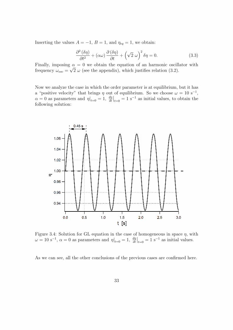
Now we analyze the case in which the order parameter is at equilibrium, but it hasa “positive velocity” that brings η out of equilibrium. So we choose ω = 10 s−1,α = 0 as parameters and η|t=0 = 1, dη
dt
∣∣t=0
= 1 s−1 as initial values, to obtain thefollowing solution:
Figure 3.4: Solution for GL equation in the case of homogeneous in space η, withω = 10 s−1, α = 0 as parameters and η|t=0 = 1, dη
dt
∣∣t=0
= 1 s−1 as initial values.
As we can see, all the other conclusions of the previous cases are confirmed here.
33
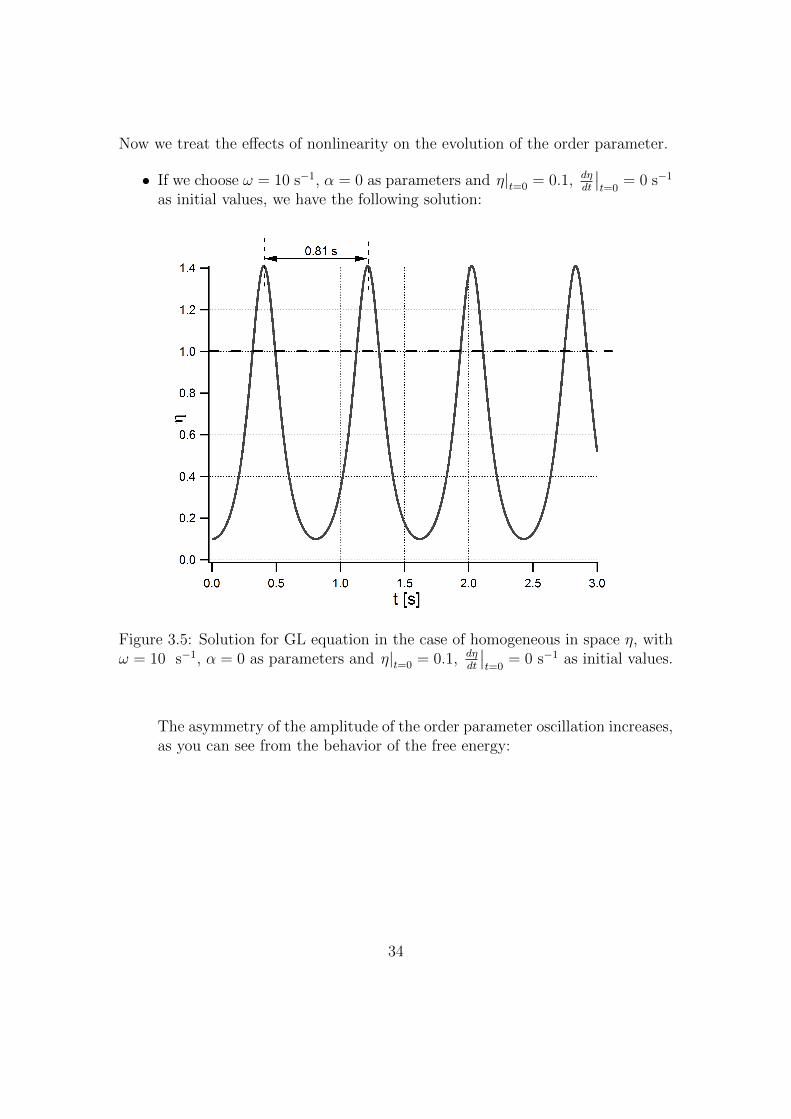
Now we treat the effects of nonlinearity on the evolution of the order parameter.
• If we choose ω = 10 s−1, α = 0 as parameters and η|t=0 = 0.1, dηdt
∣∣t=0
= 0 s−1
as initial values, we have the following solution:
Figure 3.5: Solution for GL equation in the case of homogeneous in space η, withω = 10 s−1, α = 0 as parameters and η|t=0 = 0.1, dη
dt
∣∣t=0
= 0 s−1 as initial values.
The asymmetry of the amplitude of the order parameter oscillation increases,as you can see from the behavior of the free energy:
34
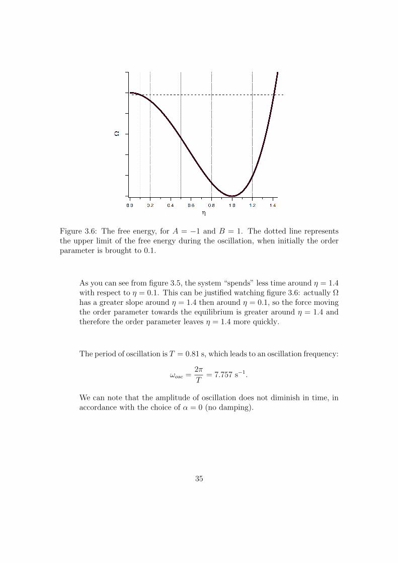
Figure 3.6: The free energy, for A = −1 and B = 1. The dotted line representsthe upper limit of the free energy during the oscillation, when initially the orderparameter is brought to 0.1.
As you can see from figure 3.5, the system “spends” less time around η = 1.4with respect to η = 0.1. This can be justified watching figure 3.6: actually Ωhas a greater slope around η = 1.4 then around η = 0.1, so the force movingthe order parameter towards the equilibrium is greater around η = 1.4 andtherefore the order parameter leaves η = 1.4 more quickly.
The period of oscillation is T = 0.81 s, which leads to an oscillation frequency:
ωosc =2π
T= 7.757 s−1.
We can note that the amplitude of oscillation does not diminish in time, inaccordance with the choice of α = 0 (no damping).
35
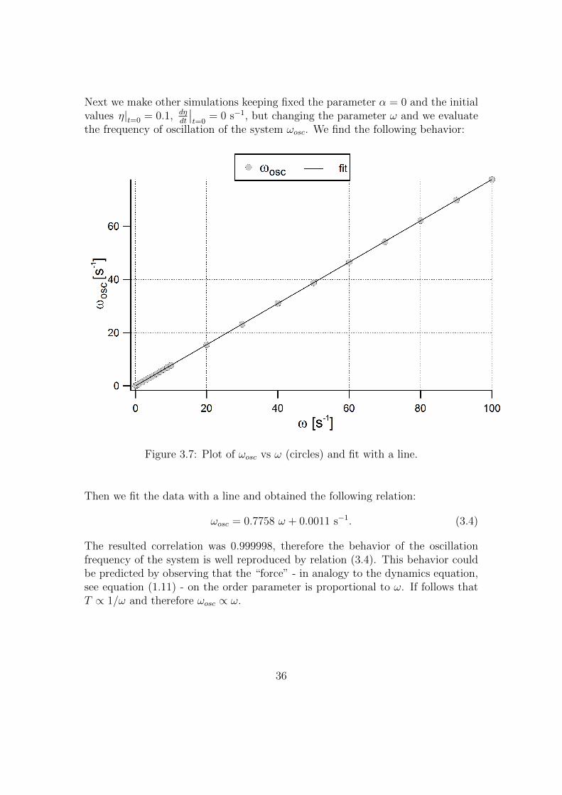
Next we make other simulations keeping fixed the parameter α = 0 and the initialvalues η|t=0 = 0.1, dη
dt
∣∣t=0
= 0 s−1, but changing the parameter ω and we evaluatethe frequency of oscillation of the system ωosc. We find the following behavior:
Figure 3.7: Plot of ωosc vs ω (circles) and fit with a line.
Then we fit the data with a line and obtained the following relation:
ωosc = 0.7758 ω + 0.0011 s−1. (3.4)
The resulted correlation was 0.999998, therefore the behavior of the oscillationfrequency of the system is well reproduced by relation (3.4). This behavior couldbe predicted by observing that the “force” - in analogy to the dynamics equation,see equation (1.11) - on the order parameter is proportional to ω. If follows thatT ∝ 1/ω and therefore ωosc ∝ ω.
36
3.1.2 Technical details
To obtain the data in Section 3.1.1 we use a “0D Model”, with a “Global ODEsand DAEs” physics. The input function is:
f(u, ut, utt) = utt + (alpha ∗ omega0) ∗ ut + ((omega0)2) ∗ (A ∗ u+B ∗ (u3)).
In COMSOL Multiphysics we used the variable omega0 standing for ω of this workand alpha standing for α of this work.The parameters and the initial values used are indicated for each graph.We use a “Time Dependent Study”, with “Generalized alpha” time steppingmethod. The steps taken by solver are manual, with time step varying from 1to 10−4, depending on the frequency we are solving for.
37
3.2 Time-independent equilibrium order param-
eter with damping
3.2.1 Results
In the current section we would like to see how the order parameter behaves if thedamping coefficient is not negligible. Therefore fix the parameters:
• A ≡ −1 (dimensionless), in order to obtain a non-zero order parameter;
• B ≡ 1 (dimensionless).
So from equation (1.10) the equilibrium value is:
ηeq =
√−AB
= 1.
Then in this section we keep fixed the parameter ω = 10 s−1 and we analyze thebehavior of the order parameter when α changes.
• If we choose ω = 10 s−1, α = 0.05 as parameters and η|t=0 = 1.1,dηdt
∣∣t=0
= 0 s−1 as initial values, we have the following solution:
38
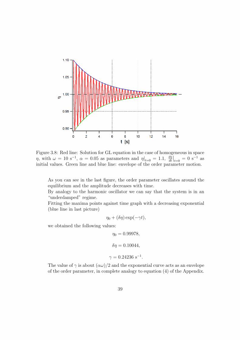
Figure 3.8: Red line: Solution for GL equation in the case of homogeneous in spaceη, with ω = 10 s−1, α = 0.05 as parameters and η|t=0 = 1.1, dη
dt
∣∣t=0
= 0 s−1 asinitial values. Green line and blue line: envelope of the order parameter motion.
As you can see in the last figure, the order parameter oscillates around theequilibrium and the amplitude decreases with time.By analogy to the harmonic oscillator we can say that the system is in an“underdamped” regime.Fitting the maxima points against time graph with a decreasing exponential(blue line in last picture)
η0 + (δη) exp(−γt),
we obtained the following values:
η0 = 0.99978,
δη = 0.10044,
γ = 0.24236 s−1.
The value of γ is about (αω)/2 and the exponential curve acts as an envelopeof the order parameter, in complete analogy to equation (4) of the Appendix.
39

• If we choose ω = 10 s−1, α = 0.2 as parameters and η|t=0 = 1.1,dηdt
∣∣t=0
= 0 s−1 as initial values, we have the following solution:
Figure 3.9: Red line: Solution for GL equation in the case of homogeneous inspace η, with ω = 10 s−1, α = 0.2 as parameters and η|t=0 = 1.1, dη
dt
∣∣t=0
= 0 s−1
as initial values. Green line and blue line: envelope of the motion of the orderparameter.
As you can see in the last figure, the order parameter oscillates around theequilibrium value and the amplitude decreases with time.This case has a damping larger than the previous case, because η reaches theequilibrium value at shorter times, as expected from the choice of a greaterα.By analogy to the harmonic oscillator we can say that the system is in an“underdamped” regime.Fitting the maxima points of η(t) with a decreasing exponential (blue linein last picture)
η0 + (δη) exp(−γt),
40
we obtained the following values:
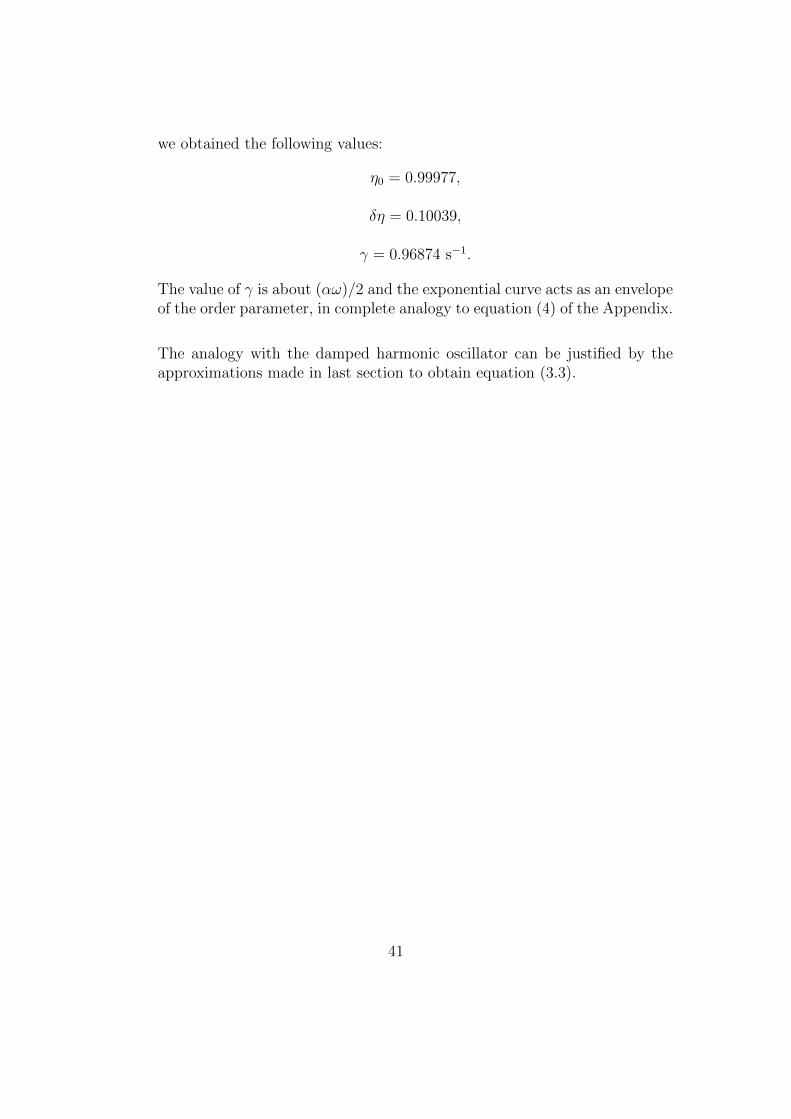
η0 = 0.99977,
δη = 0.10039,
γ = 0.96874 s−1.
The value of γ is about (αω)/2 and the exponential curve acts as an envelopeof the order parameter, in complete analogy to equation (4) of the Appendix.
The analogy with the damped harmonic oscillator can be justified by theapproximations made in last section to obtain equation (3.3).
41
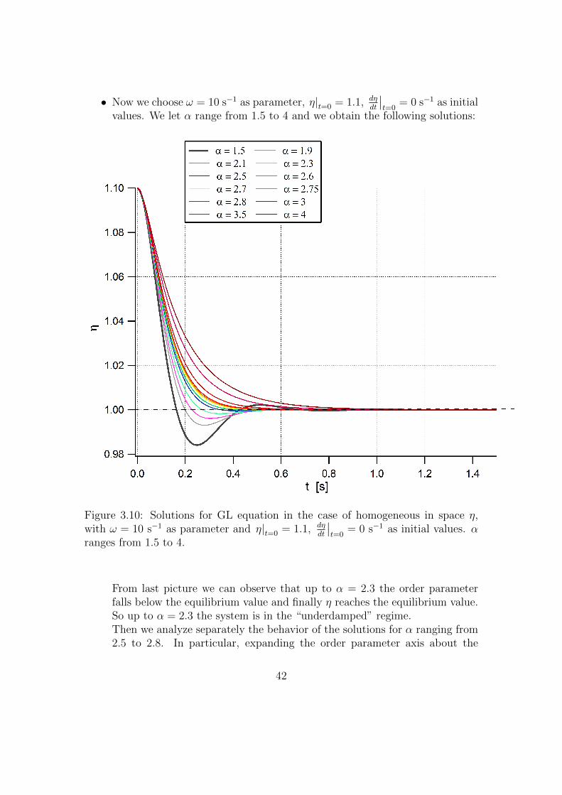
• Now we choose ω = 10 s−1 as parameter, η|t=0 = 1.1, dηdt
∣∣t=0
= 0 s−1 as initialvalues. We let α range from 1.5 to 4 and we obtain the following solutions:
Figure 3.10: Solutions for GL equation in the case of homogeneous in space η,with ω = 10 s−1 as parameter and η|t=0 = 1.1, dη
dt
∣∣t=0
= 0 s−1 as initial values. αranges from 1.5 to 4.
From last picture we can observe that up to α = 2.3 the order parameterfalls below the equilibrium value and finally η reaches the equilibrium value.So up to α = 2.3 the system is in the “underdamped” regime.Then we analyze separately the behavior of the solutions for α ranging from2.5 to 2.8. In particular, expanding the order parameter axis about the
42
equilibrium value, we obtain the following solutions:
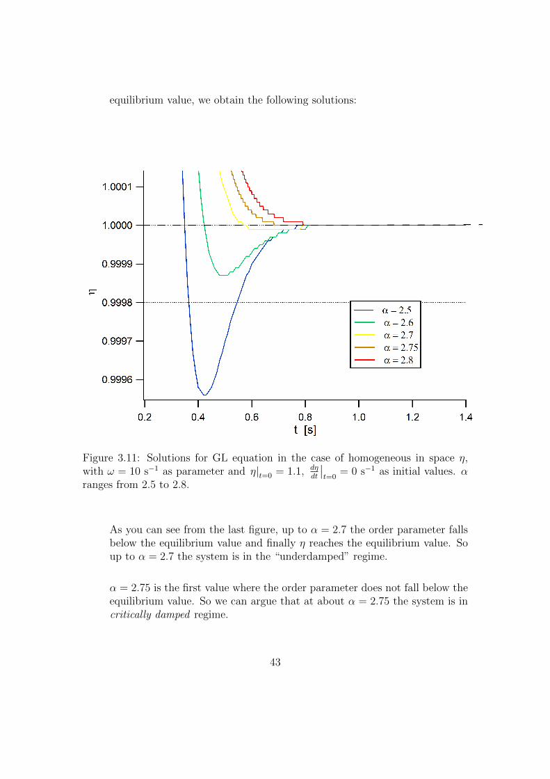
Figure 3.11: Solutions for GL equation in the case of homogeneous in space η,with ω = 10 s−1 as parameter and η|t=0 = 1.1, dη
dt
∣∣t=0
= 0 s−1 as initial values. αranges from 2.5 to 2.8.
As you can see from the last figure, up to α = 2.7 the order parameter fallsbelow the equilibrium value and finally η reaches the equilibrium value. Soup to α = 2.7 the system is in the “underdamped” regime.
α = 2.75 is the first value where the order parameter does not fall below theequilibrium value. So we can argue that at about α = 2.75 the system is incritically damped regime.
43
Reminding that choosing ω = 10 s−1 the system has an oscillation frequencyof ωosc = 13.96 s−1, we notice that the case of critically damped regime fallswhen αω is about 2 times ωosc, in perfect agreement with the theory ofdamped harmonic oscillator.
Finally, the cases α = 3 and α = 4 represent the overdamped harmonicoscillator regime.
3.2.2 Technical details
To obtain the data in Section 3.2.1 we use a “0D Model”, with a “Global ODEsand DAEs” physics. The input function is:
f(u, ut, utt) = utt + (alpha ∗ omega0) ∗ ut + ((omega0)2) ∗ (A ∗ u+B ∗ (u3)).
In COMSOL Multiphysics we used the variable omega0 standing for ω of this workand alpha standing for α of this work.The parameters and the initial values used are indicated for each graph.We use a “Time Dependent Study”, with “Generalized alpha” time steppingmethod. The steps taken by solver are manual, with a time step of 10−3.
44
3.3 Time-dependent equilibrium order parame-
ter with no damping
3.3.1 Results
In this section we analyze the behavior of the order parameter if the equilibriumvalue changes with time. Therefore we suppose that for t < 0 s the system hasthe parameters A = −1 and B = 1, so the order parameter is in equilibrium atthe value η = 1.Then at time t = 0 s a laser pulse hits the system changing the properties. Inparticular we suppose that the system is brought in another state with anothervalue for the equilibrium parameter, obtained changing the value of A.Then, for t > 0 the system tends to return in the initial state, so the coefficient Acan be thought as time dependent.In this section we choose:
A(t) =
−1 for t < 0 s
−1 + de−t/τ for t > 0 s
with d < 1, so the system supports an order parameter; this coefficient isdimensionless.
B = 1 (dimensionless), ∀t.
τ represents the temporal scale for the system to return in the initial state.
We solve GL equation for t > 0 s, and the behavior of the order parameter fornegative times is represented by choosing η|t=0 = 1, dη
dt
∣∣t=0
= 0 s−1 as initial values.
We analyze the following cases:
45
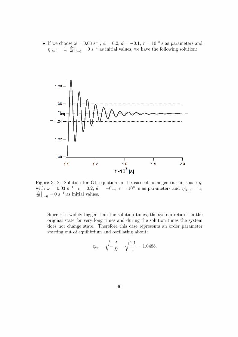
• If we choose ω = 0.03 s−1, α = 0.2, d = −0.1, τ = 1010 s as parameters andη|t=0 = 1, dη
dt
∣∣t=0
= 0 s−1 as initial values, we have the following solution:
Figure 3.12: Solution for GL equation in the case of homogeneous in space η,with ω = 0.03 s−1, α = 0.2, d = −0.1, τ = 1010 s as parameters and η|t=0 = 1,dηdt
∣∣t=0
= 0 s−1 as initial values.
Since τ is widely bigger than the solution times, the system returns in theoriginal state for very long times and during the solution times the systemdoes not change state. Therefore this case represents an order parameterstarting out of equilibrium and oscillating about:
ηeq =
√−AB
=
√1.1
1= 1.0488.
46
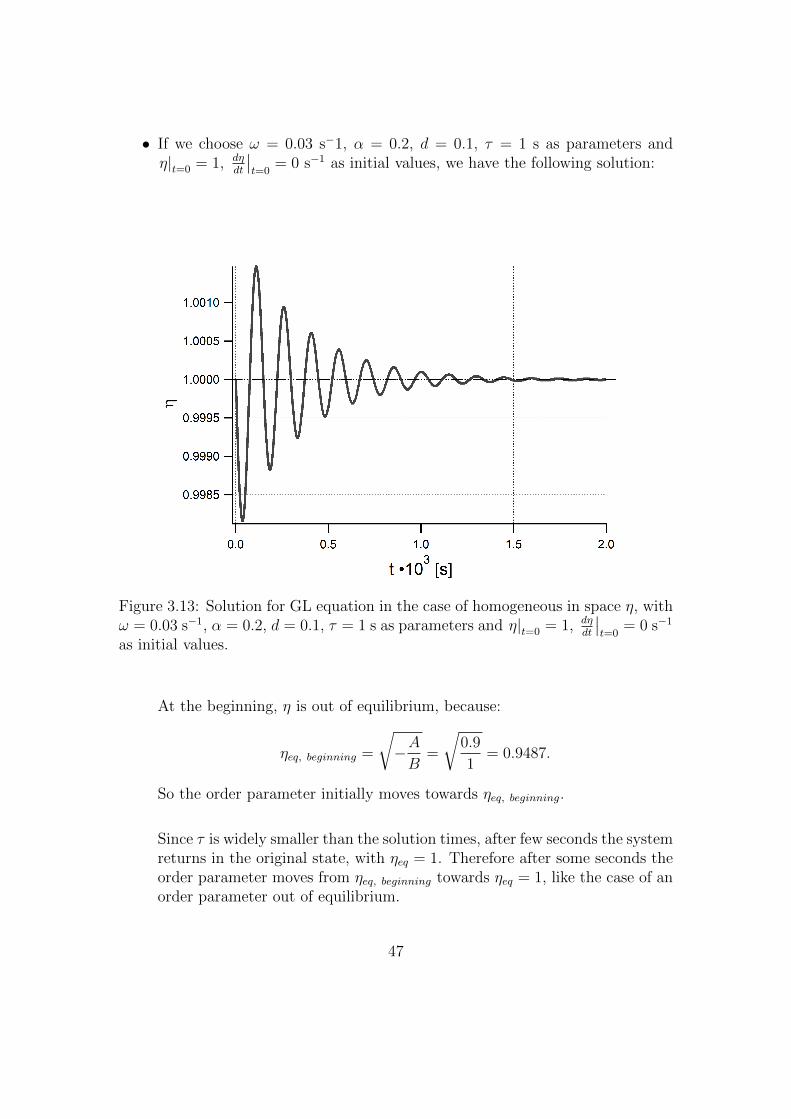
• If we choose ω = 0.03 s−1, α = 0.2, d = 0.1, τ = 1 s as parameters andη|t=0 = 1, dη
dt
∣∣t=0
= 0 s−1 as initial values, we have the following solution:
Figure 3.13: Solution for GL equation in the case of homogeneous in space η, withω = 0.03 s−1, α = 0.2, d = 0.1, τ = 1 s as parameters and η|t=0 = 1, dη
dt
∣∣t=0
= 0 s−1
as initial values.
At the beginning, η is out of equilibrium, because:
ηeq, beginning =
√−AB
=
√0.9
1= 0.9487.
So the order parameter initially moves towards ηeq, beginning.
Since τ is widely smaller than the solution times, after few seconds the systemreturns in the original state, with ηeq = 1. Therefore after some seconds theorder parameter moves from ηeq, beginning towards ηeq = 1, like the case of anorder parameter out of equilibrium.
47

• If we choose ω = 0.03 s−1, α = 0.2, d = −0.1, τ = 200 s as parameters andη|t=0 = 1, dη
dt
∣∣t=0
= 0 s−1 as initial values, we have the following solution:
Figure 3.14: Solution for GL equation in the case of homogeneous in space η,with ω = 0.03 s−1, α = 0.2, d = −0.1, τ = 200 s as parameters and η|t=0 = 1,dηdt
∣∣t=0
= 0 s−1 as initial values.
At the beginning, η is out of equilibrium, because:
ηeq, beginning =
√−AB
=
√1.1
1= 1.0488.
So the order parameter initially oscillates about ηeq, beginning.
Finally, when the time is widely larger than τ the system returns in theoriginal state, with ηeq = 1. Therefore for long times η oscillates aboutηeq = 1, like the case of an order parameter out of equilibrium.
This is an intermediate case with respect to the two previous limiting cases.
48

3.3.2 Technical details
To obtain the data in Section 3.3.1 we use a “0D Model”, with a “Global ODEsand DAEs” physics. The input function is:
f(u, ut, utt) = utt + (alpha ∗ omega0) ∗ ut + ((omega0)2) ∗ (A ∗ u+B ∗ (u3)),
with:A = A0 ∗ (1− d ∗ exp(−t/tau)).
A0 = −1 fixed.
In COMSOL Multiphysics we used the variable omega0 standing for ω of thiswork, alpha standing for α of this work and tau standing for τ of this work.The parameters and the initial values used are indicated for each graph.We use a “Time Dependent Study”, with “Generalized alpha” time steppingmethod. The steps taken by solver are manual, with a time step of 10−3 forthe case with τ = 1010 s, of 1 for the case with τ = 1 s and of 0.1 for the case withτ = 200 s.
References
1. Massimo Capone, Michele Fabrizio, Daniele Fausti, Claudio Giannetti, Ful-vio Parmigiani, Ultrafast optical spectroscopy of strongly-correlated materi-als and high-temperature superconductors: a non-equilibrium approach, Ad-vances in Physics Vol. 00, No. 00, June 2008, 1-36.
49

Chapter 4
Reflectivity for a system inoverdamped regime
In this chapter we simulate a cylindrical system, brought out of equilibrium bya laser pulse, and we discuss the dynamics of the order parameter. We supposethat the energy received from the laser pulse is diffused in the system and thengiven to the thermal bath surrounding the cylinder. Therefore we have to dealwith an overdamped regime, in which the propagation of the order parameter isincoherent.Finally we use simulations data to reproduce reflectivity behavior of a supercon-ductor sample.
In this chapter we try to solve numerically GL equation for real order parameter:
1
ω2
∂2η
∂t2+(αω
) ∂η∂t
+ A(P, T )η +B(P )η3 − λ∇2η = 0
using “COMSOL Multiphysics” software, in the case of an overdamped system.Therefore we choose the following parameters:
• ω = 10 s−1;
• α = 103 (dimensionless), so the term of the second derivate with respect totime becomes negligible with respect to the term of the first derivate. Thiscondition makes the overdamped regime;
• λ = 0.1 m2;
• A = −1 (dimensionless), so the system supports an order parameter;
• B = 1 (dimensionless).
50
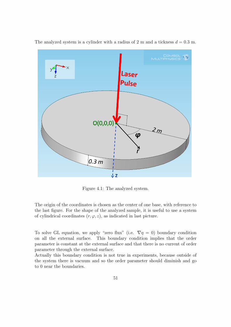
The analyzed system is a cylinder with a radius of 2 m and a tickness d = 0.3 m.
Figure 4.1: The analyzed system.
The origin of the coordinates is chosen as the center of one base, with reference tothe last figure. For the shape of the analyzed sample, it is useful to use a systemof cylindrical coordinates (r, ϕ, z), as indicated in last picture.
To solve GL equation, we apply “zero flux” (i.e. ∇η = 0) boundary conditionon all the external surface. This boundary condition implies that the orderparameter is constant at the external surface and that there is no current of orderparameter through the external surface.Actually this boundary condition is not true in experiments, because outside ofthe system there is vacuum and so the order parameter should diminish and goto 0 near the boundaries.
51

However we choose zero flux boundary condition because it is very easy toimplement and to obtain a solution; furthermore it is a good approximation toreality for the initial times, when the perturbation of order parameter has notreached the boundaries yet.With this condition the order parameter at equilibrium is ηeq ≡ 1 over all thesystem.
For negative times t < 0 s we suppose that a laser pulse hits the base with coordi-nate z = 0 m and excites the system, as depicted in figure 4.1. Then at time t = 0 sthe laser pulse is turned off, so that the initial values for the order parameter are:
η|t=0 = 1− I exp
(− z
lpen
)exp
(− r2
l2width
); (4.1)
dη
dt
∣∣∣∣t=0
= 0 s−1. (4.2)
Initial value (4.1) tells us that for negative times (t < 0 s) a laser pulse adds aperturbation to the equilibrium order parameter (ηeq ≡ 1).The laser pulse hits the system on the base with coordinate z = 0 m and theperturbation decreases exponentially as we go inside the sample. lpen representsthe spatial scale over which the order parameter returns to the equilibrium value.The perturbation has a rotational symmetry, so we can use a 2D-axisymmetricgeometry and study the behavior of the order parameter on a half-plane (r, z)with ϕ fixed. Thanks to this symmetry, it does not matter the choice of theparticular value of ϕ.The perturbation has and a gaussian shape, with the z axis as center and lwidthas width.
In this chapter we analyze the behavior of the system for different values of lpenand of the parameter I (representing the intensity of the laser pulse), while wewill hold fixed the parameter lwidth = 0.5 m.
Initial value (4.2) means that the laser pulse brings the system in anotherequilibrium state. So the system does not move until the laser is turned off (att = 0 s) and at t = 0 s the order parameter as a negligible “velocity” (in analogyto the dynamics equation).For t > 0 s the system moves towards the equilibrium state with η = ηeq ≡ 1.
52
When the order parameter in a certain point of the system changes, the reflectivity(R) in that point changes.
In particular, introducing δη = η−ηeq (as explained in section 1.4), we can assumethat the following relation holds:
R = γ |δη| , (4.3)
where γ is a constant.
This relation allows us to predict the reflectivity of the system behavior when weknow δη.
After analyzing the behavior of the order parameter in some interesting case, inthis chapter we compare experimental reflectivities with data from the solution ofGL equation, obtained with COMSOL Multiphysics.
53

4.1 Results
4.1.1 Homogeneous excitation
This case is when lpen is larger than the thickness of the system in the z direction;therefore δη is almost equal in z direction at the initial times.In particular we solved GL equation for the case lpen = 100 m (we remind thatthe thickness of the system in z direction is d = 0.3 m).Letting I assume several values, we analyze a few cases. For each value of theparameter I we make a simulation.
Choosing I = 0 (i.e. no laser applied for t < 0 s), we verify that the system staysforever in the equilibrium value ηeq ≡ 1:
Figure 4.2: The solution for lpen = 100 m and I = 0, for all times. The color scalerepresents the value of η.
Since I = 0, we can notice that this result does not depend on the particular choiceof lpen.
54
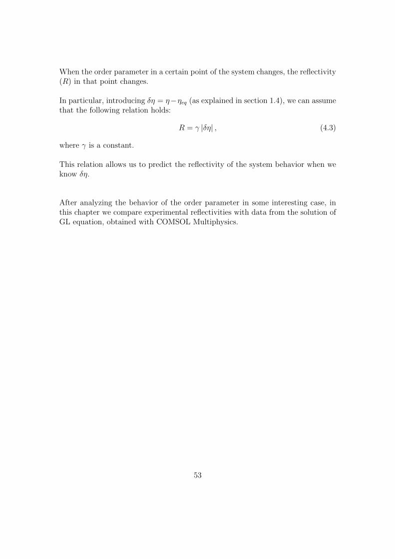
Choosing I = 0.8 the order parameter changes so:
Figure 4.3: The solution for lpen = 100 m and I = 0.8, for t = 0 s. The color scalerepresents the value of η.
Figure 4.4: The solution for lpen = 100 m and I = 0.8, for t = 30 s. The colorscale represents the value of η.
55
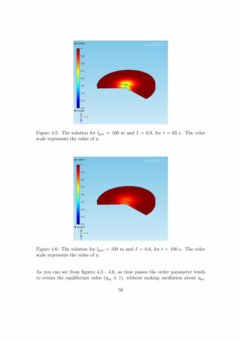
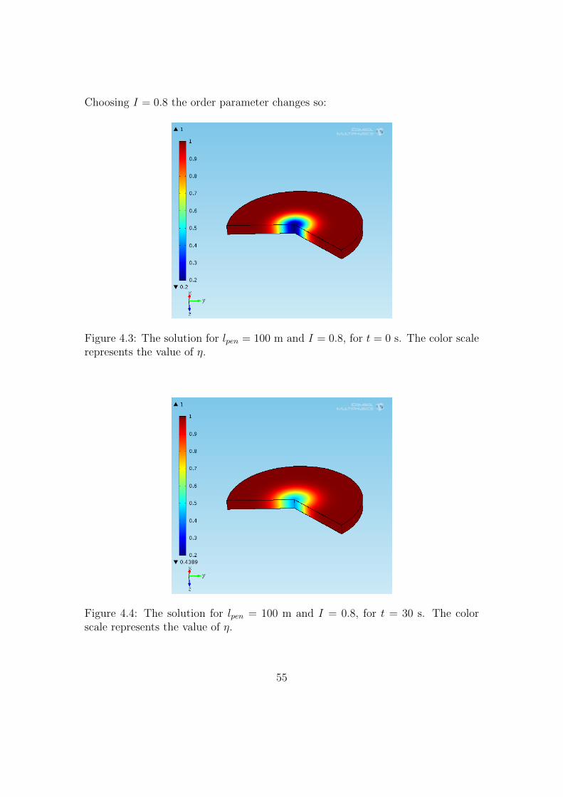
Figure 4.5: The solution for lpen = 100 m and I = 0.8, for t = 60 s. The colorscale represents the value of η.
Figure 4.6: The solution for lpen = 100 m and I = 0.8, for t = 100 s. The colorscale represents the value of η.
As you can see from figures 4.3 - 4.6, as time passes the order parameter tendsto return the equilibrium value (ηeq ≡ 1), without making oscillation about ηeq.
56

This behavior is typical of the overdamped regime.We can also note that the order parameter is actually constant in z direction. Inthis particular case the equation reduces to a diffusion equation.
When the intensity of laser pulse increases and is greater than 1, the initial valuedescribed by (4.1) is no more correct because this would imply a negative orderparameter in a certain domain at t = 0 s. For a fixed ϕ, in the half-plane (r, z)the order parameter would be positive in Ω1 domain and negative in Ω2 domain,with reference to figure 4.7.
Figure 4.7: The half-plane (r, z), for a fixed ϕ.
σ would be the line where the order parameter is 0. So from condition (4.1):
I exp
(− z
lpen
)exp
(− r2
l2width
)= 1.
Taking the logarithm we have:
z
lpen+
r2
l2width= ln I,
and this can be written as:
z = −(lpenl2width
)r2 + (ln I) lpen. (4.4)
So we proved that σ is defined by (4.4), which is the equation of a parabola.
57
Therefore we split the half-plane (r, z) in 2 domains, defined in figure 4.7 and byrelation (4.4), and we apply the following initial values condition:
η|t=0 =
1− I exp
(− z
lpen
)exp
(− r2
l2width
)for (r, z) in Ω1
0 for (r, z) in Ω2
(4.5)
dη
dt
∣∣∣∣t=0
= 0 s−1 everywhere. (4.6)
With this condition we analyze a few cases with a high intensity laser.
Now we would like to evaluate the reflectivity of the system in the region wherethe laser effects are high. To obtain this, we make an average of the orderparameter along a line, defined by the coordinate r = 0 m (where there is thecenter of the gaussian pulse). The line starts at z = 0 m and is not longer thanlpen (in this region the laser effects are high).In the particular case of the current section, where the height of the cylinder d ismuch shorter than lpen, z coordinate of the average line ranges from the beginningto the end of the cylinder.Finally, to obtain |< δη >| (the average of δη with positive sign), we subtractηeq ≡ 1 to the average order parameter and take the positive sign.
|< δη >| is a function of the laser intensity I and of the time.
From the definitions above, we are able to evaluate the expression of |< δη >| att = 0 s analytically.As stated before, we make the average on a line ranging from z = 0 m to z = w(we use w to cover all the possible cases: w can be either the end of the cylinderd or lpen). Using relations (4.1), (4.4) and (4.5) we have 3 different cases:
• I ≤ 1. In this case relation (4.1) holds over all the average line:
|< δη(t = 0 s) >| = |< η(t = 0 s)− ηeq >| =
=
∣∣∣∣ 1
w
∫ w
0
[η(t = 0 s, r = 0 m, z)− ηeq] dz∣∣∣∣ =
58
=
∣∣∣∣ Iw∫ w
0
exp
(− z
lpen
)dz
∣∣∣∣ =lpenw
[1− exp
(− w
lpen
)]I. (4.7)
• 1 < I ≤ exp (w/lpen). In this case the average line lies in 2 domains (theaverage line lies completely in Ω1 domain at the limit value I = exp (w/lpen)),so we have to make the average using relation (4.5):
|< δη(t = 0 s) >| = |< η(t = 0 s)− ηeq >| =
=
∣∣∣∣ 1
w
∫ w
0
[η(t = 0 s, r = 0 m, z)− ηeq] dz∣∣∣∣ =
=
∣∣∣∣∣− 1
w
∫ (ln I)lpen
0
dz − I
w
∫ w
(ln I)lpen
exp
(− z
lpen
)dz
∣∣∣∣∣ =
=
∣∣∣∣−(ln I)lpenw
+lpenI
w
exp
(− w
lpen
)− exp
[−(ln I)lpen
lpen
]∣∣∣∣ =
=lpenw
∣∣∣∣1 + (ln I)− I exp
(− w
lpen
)∣∣∣∣ =
=lpenw
[1 + (ln I)− I exp
(− w
lpen
)]. (4.8)
The last equality follows from the fact that in this range of intensity,I exp (−w/lpen) ranges from 0 to 1 and so
1 + (ln I)− I exp (−w/lpen)
is always positive.
In the case of I → 1 expression (4.8) reduces to expression (4.7). Thereforethe general expression of |< δη >| is continuous at I = 1.
Evidently expression (4.8) increases, reaching the limiting value of 1 ifI → exp (w/lpen).
• I > exp (w/lpen). In this case the average line lies completely in Ω1 domain.Therefore:
|< δη(t = 0 s) >| = |< η(t = 0 s)− ηeq >| =
=
∣∣∣∣ 1
w
∫ w
0
[η(t = 0 s, r = 0 m, z)− ηeq] dz∣∣∣∣ =
∣∣∣∣− 1
w
∫ w
0
dz
∣∣∣∣ = 1. (4.9)
59
This case is reached when the laser is so intense that the order parameterhas been brought to 0 over all the average line (saturation).
Increasing the laser intensity, δη does not change further over the averageline.
Evidently the general expression of |< δη >| is continuous at
I = exp (w/lpen) .
Consequently we have just obtained a continuous expression for |< δη >| at t = 0 s:
|< δη(t = 0 s) >| =
lpenw
[1− exp
(− w
lpen
)]I (4.7) for I ≤ 1
lpenw
∣∣∣∣1 + (ln I)− I exp
(− w
lpen
)∣∣∣∣ (4.8) for 1 < I ≤ exp
(w
lpen
)
1 (4.9) for I > exp
(w
lpen
).
As you can see, for t = 0 s and w = lpen (laser penetration lower than the cylinderthickness), |< δη >| does not depend on the particular choice of lpen.
Furthermore it is worth to notice that the general expression of |< δη >| is alwayscontinuous for every laser intensity.
60
Now we make a few simulations changing the value of I and for each value of I weevaluate the line average. Here we report the results obtained:
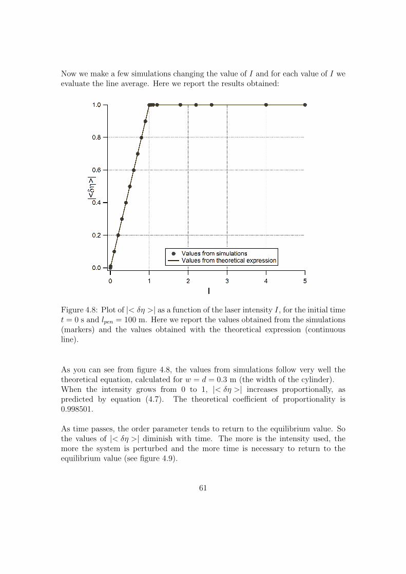
Figure 4.8: Plot of |< δη >| as a function of the laser intensity I, for the initial timet = 0 s and lpen = 100 m. Here we report the values obtained from the simulations(markers) and the values obtained with the theoretical expression (continuousline).
As you can see from figure 4.8, the values from simulations follow very well thetheoretical equation, calculated for w = d = 0.3 m (the width of the cylinder).When the intensity grows from 0 to 1, |< δη >| increases proportionally, aspredicted by equation (4.7). The theoretical coefficient of proportionality is0.998501.
As time passes, the order parameter tends to return to the equilibrium value. Sothe values of |< δη >| diminish with time. The more is the intensity used, themore the system is perturbed and the more time is necessary to return to theequilibrium value (see figure 4.9).
61

Figure 4.9: Plot of |< δη >| as a function of the laser intensity I, for differenttimes and lpen = 100 m. These results are obtained from simulations.
62
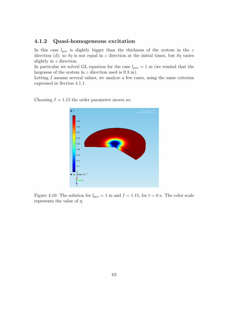
4.1.2 Quasi-homogeneous excitation
In this case lpen is slightly bigger than the thickness of the system in the zdirection (d); so δη is not equal in z direction at the initial times, but δη variesslightly in z direction.In particular we solved GL equation for the case lpen = 1 m (we remind that thelargeness of the system in z direction used is 0.3 m).Letting I assume several values, we analyze a few cases, using the same criterionexpressed in Section 4.1.1.
Choosing I = 1.15 the order parameter moves so:
Figure 4.10: The solution for lpen = 1 m and I = 1.15, for t = 0 s. The color scalerepresents the value of η.
63

Figure 4.11: The solution for lpen = 1 m and I = 1.15, for t = 30 s. The colorscale represents the value of η.
As you can see from figures 4.10 - 4.11, as time passes the order parameter tendsto return to the equilibrium value (ηeq ≡ 1), without making oscillation about ηeq.This behavior is typical of the overdamped regime.We can also note that the order parameter does not have significative variationsin z direction.
As anticipated in Section 4.1.1, we would like to evaluate the reflectivity of thesystem in the region where the laser effects are high. To obtain this, we make anaverage of the order parameter along a line, starting at (r = 0 m, z = 0 m) andfinishing at (r = 0 m, z = w).In the particular case of the current section, where the thickness d of the cylinderis shorter than lpen, we choose w = d.As for |< δη >|, all the considerations expressed in Section 4.1.1 holds.
64
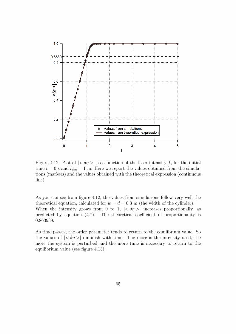
Figure 4.12: Plot of |< δη >| as a function of the laser intensity I, for the initialtime t = 0 s and lpen = 1 m. Here we report the values obtained from the simula-tions (markers) and the values obtained with the theoretical expression (continuousline).
As you can see from figure 4.12, the values from simulations follow very well thetheoretical equation, calculated for w = d = 0.3 m (the width of the cylinder).When the intensity grows from 0 to 1, |< δη >| increases proportionally, aspredicted by equation (4.7). The theoretical coefficient of proportionality is0.863939.
As time passes, the order parameter tends to return to the equilibrium value. Sothe values of |< δη >| diminish with time. The more is the intensity used, themore the system is perturbed and the more time is necessary to return to theequilibrium value (see figure 4.13).
65
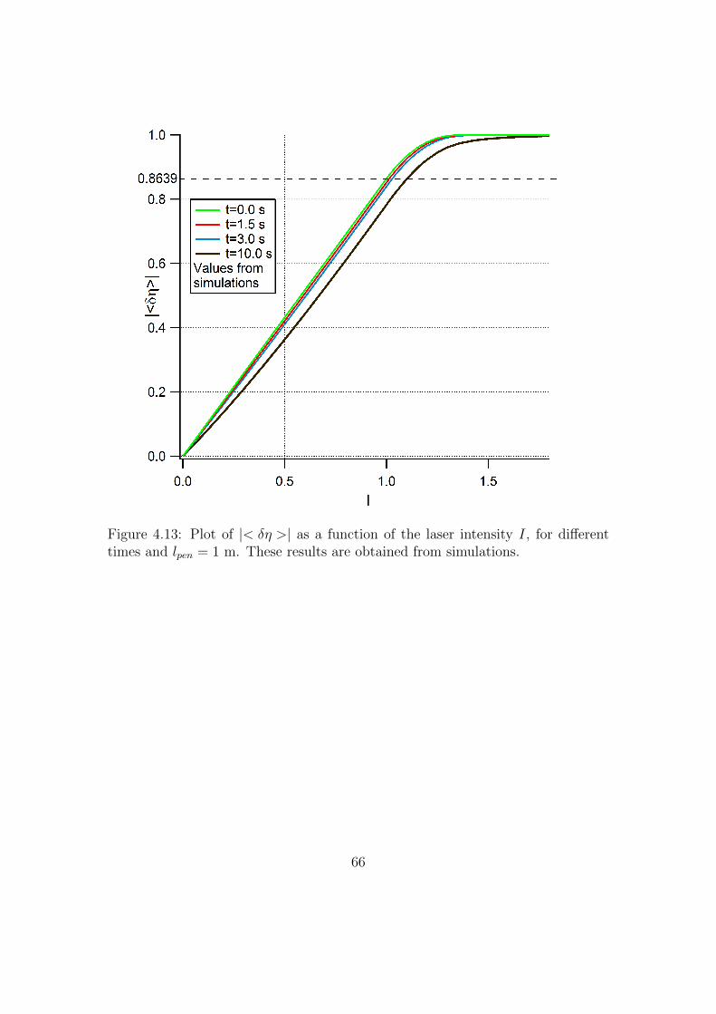
Figure 4.13: Plot of |< δη >| as a function of the laser intensity I, for differenttimes and lpen = 1 m. These results are obtained from simulations.
66

4.1.3 Strongly inhomogeneous excitation
In this case lpen is shorter than the thickness of the system in the z direction(d); so δη varies a lot in z direction, reaching the value of 0 near one end of thecylinder. Therefore this case is representative of the bulk system, in which thelaser does not penetrate in the system.In particular we solved GL equation for the case lpen = 0.1 m (we remind that thelargeness of the system in z direction used is d = 0.3 m).Letting I assume several values, we analyze a few cases, using the same criterionexpressed in Section 4.1.1.
Choosing I = 1.5 the order parameter moves so:
Figure 4.14: The solution for lpen = 0.1 m and I = 1.5, for t = 0 s. The color scalerepresents the value of η.
67
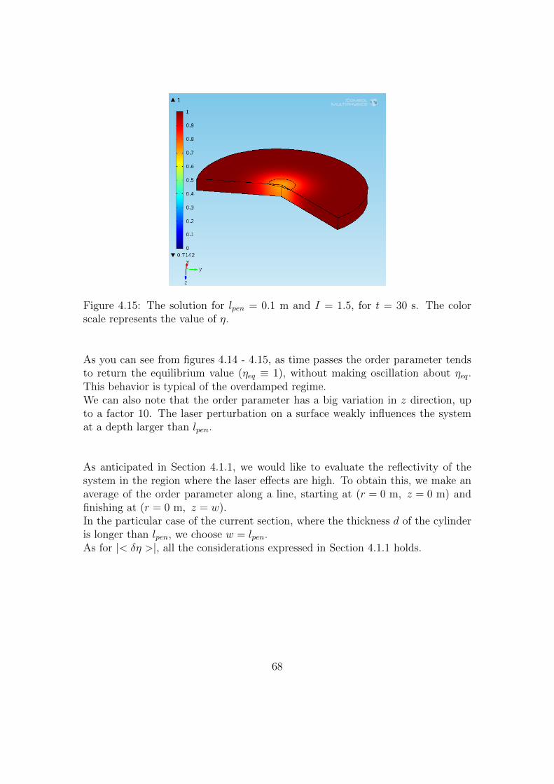
Figure 4.15: The solution for lpen = 0.1 m and I = 1.5, for t = 30 s. The colorscale represents the value of η.
As you can see from figures 4.14 - 4.15, as time passes the order parameter tendsto return the equilibrium value (ηeq ≡ 1), without making oscillation about ηeq.This behavior is typical of the overdamped regime.We can also note that the order parameter has a big variation in z direction, upto a factor 10. The laser perturbation on a surface weakly influences the systemat a depth larger than lpen.
As anticipated in Section 4.1.1, we would like to evaluate the reflectivity of thesystem in the region where the laser effects are high. To obtain this, we make anaverage of the order parameter along a line, starting at (r = 0 m, z = 0 m) andfinishing at (r = 0 m, z = w).In the particular case of the current section, where the thickness d of the cylinderis longer than lpen, we choose w = lpen.As for |< δη >|, all the considerations expressed in Section 4.1.1 holds.
68
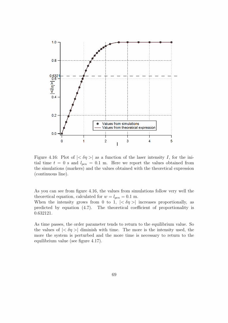
Figure 4.16: Plot of |< δη >| as a function of the laser intensity I, for the ini-tial time t = 0 s and lpen = 0.1 m. Here we report the values obtained fromthe simulations (markers) and the values obtained with the theoretical expression(continuous line).
As you can see from figure 4.16, the values from simulations follow very well thetheoretical equation, calculated for w = lpen = 0.1 m.When the intensity grows from 0 to 1, |< δη >| increases proportionally, aspredicted by equation (4.7). The theoretical coefficient of proportionality is0.632121.
As time passes, the order parameter tends to return to the equilibrium value. Sothe values of |< δη >| diminish with time. The more is the intensity used, themore the system is perturbed and the more time is necessary to return to theequilibrium value (see figure 4.17).
69
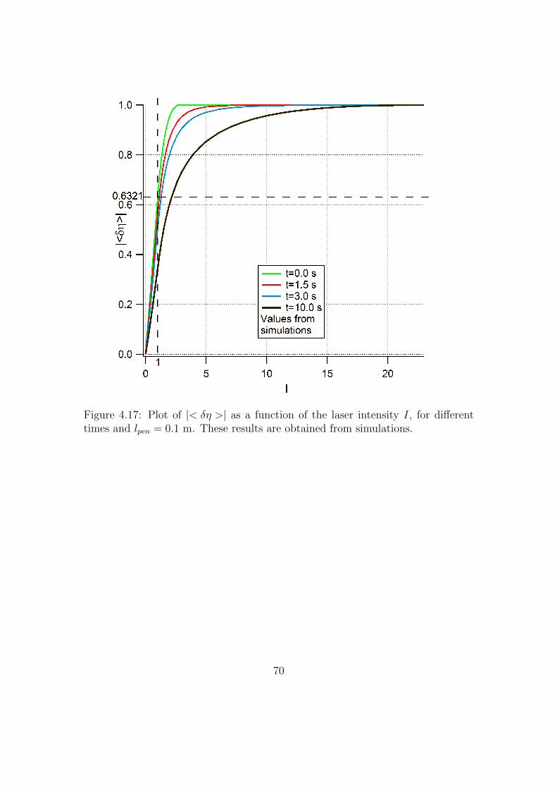
Figure 4.17: Plot of |< δη >| as a function of the laser intensity I, for differenttimes and lpen = 0.1 m. These results are obtained from simulations.
70

4.1.4 Bulk system
In this case lpen is much shorter than the thickness of the system in the z direction(d); so at the initial time δη varies a lot in z direction, reaching a value close to 0inside the cylinder. Therefore in this case we have the bulk system.In particular we solved GL equation for the case lpen = 0.03 m (we remind thatthe thickness of the system in z direction used is d = 0.3 m).Letting I assume several values, we analyze a few cases, using the same criterionexpressed in Section 4.1.1.
Choosing I = 2.6 the order parameter moves so:
Figure 4.18: The solution for lpen = 0.03 m and I = 2.6, for t = 0 s. The colorscale represents the value of η.
71
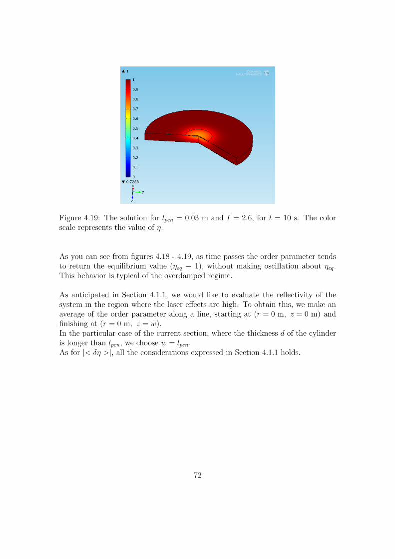
Figure 4.19: The solution for lpen = 0.03 m and I = 2.6, for t = 10 s. The colorscale represents the value of η.
As you can see from figures 4.18 - 4.19, as time passes the order parameter tendsto return the equilibrium value (ηeq ≡ 1), without making oscillation about ηeq.This behavior is typical of the overdamped regime.
As anticipated in Section 4.1.1, we would like to evaluate the reflectivity of thesystem in the region where the laser effects are high. To obtain this, we make anaverage of the order parameter along a line, starting at (r = 0 m, z = 0 m) andfinishing at (r = 0 m, z = w).In the particular case of the current section, where the thickness d of the cylinderis longer than lpen, we choose w = lpen.As for |< δη >|, all the considerations expressed in Section 4.1.1 holds.
72

Figure 4.20: Plot of |< δη >| as a function of the laser intensity I, for the ini-tial time t = 0 s and lpen = 0.03 m. Here we report the values obtained fromthe simulations (markers) and the values obtained with the theoretical expression(continuous line).
As you can see from last picture, the values from simulations follow very well thetheoretical equation, calculated for w = lpen = 0.03 m.When the intensity grows from 0 to 1, |< δη >| increases proportionally, aspredicted by equation (4.7). The theoretical coefficient of proportionality is0.632121.
As time passes, the order parameter tends to return to the equilibrium value. Sothe values of |< δη >| diminish with time. The more intensity used, the more thesystem is perturbed, the more time is necessary to return to the equilibrium value(see figure 4.21).
73
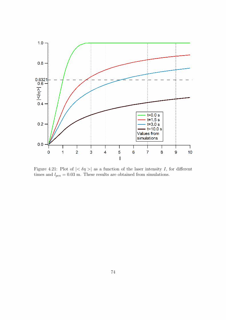
Figure 4.21: Plot of |< δη >| as a function of the laser intensity I, for differenttimes and lpen = 0.03 m. These results are obtained from simulations.
74
4.1.5 Comparison of the analyzed cases
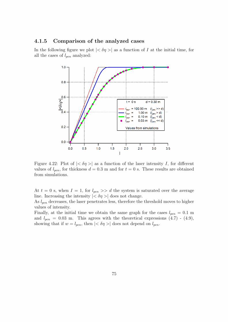
In the following figure we plot |< δη >| as a function of I at the initial time, forall the cases of lpen analyzed:
Figure 4.22: Plot of |< δη >| as a function of the laser intensity I, for differentvalues of lpen, for thickness d = 0.3 m and for t = 0 s. These results are obtainedfrom simulations.
At t = 0 s, when I = 1, for lpen >> d the system is saturated over the averageline. Increasing the intensity |< δη >| does not change.As lpen decreases, the laser penetrates less, therefore the threshold moves to highervalues of intensity.Finally, at the initial time we obtain the same graph for the cases lpen = 0.1 mand lpen = 0.03 m. This agrees with the theoretical expressions (4.7) - (4.9),showing that if w = lpen, then |< δη >| does not depend on lpen.
75
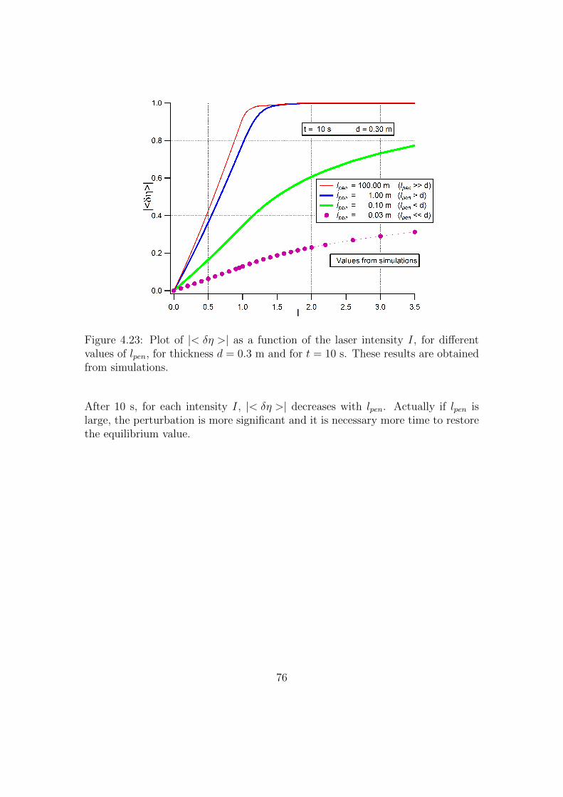
Figure 4.23: Plot of |< δη >| as a function of the laser intensity I, for differentvalues of lpen, for thickness d = 0.3 m and for t = 10 s. These results are obtainedfrom simulations.
After 10 s, for each intensity I, |< δη >| decreases with lpen. Actually if lpen islarge, the perturbation is more significant and it is necessary more time to restorethe equilibrium value.
76
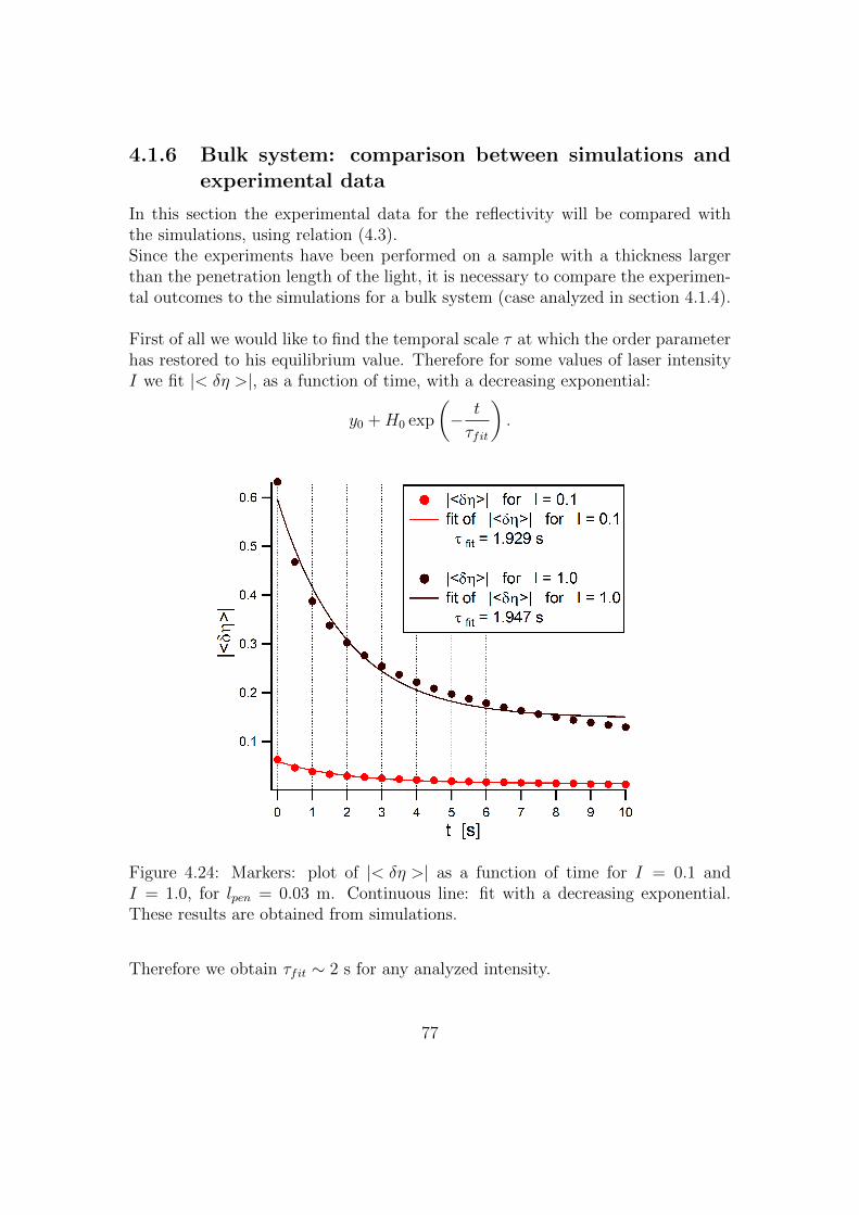
4.1.6 Bulk system: comparison between simulations andexperimental data
In this section the experimental data for the reflectivity will be compared withthe simulations, using relation (4.3).Since the experiments have been performed on a sample with a thickness largerthan the penetration length of the light, it is necessary to compare the experimen-tal outcomes to the simulations for a bulk system (case analyzed in section 4.1.4).
First of all we would like to find the temporal scale τ at which the order parameterhas restored to his equilibrium value. Therefore for some values of laser intensityI we fit |< δη >|, as a function of time, with a decreasing exponential:
y0 +H0 exp
(− t
τfit
).
Figure 4.24: Markers: plot of |< δη >| as a function of time for I = 0.1 andI = 1.0, for lpen = 0.03 m. Continuous line: fit with a decreasing exponential.These results are obtained from simulations.
Therefore we obtain τfit ∼ 2 s for any analyzed intensity.
77
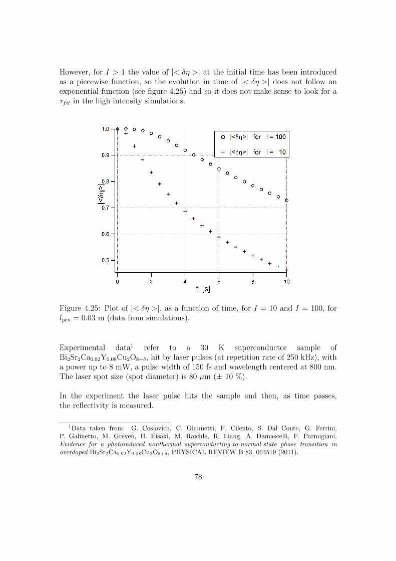
However, for I > 1 the value of |< δη >| at the initial time has been introducedas a piecewise function, so the evolution in time of |< δη >| does not follow anexponential function (see figure 4.25) and so it does not make sense to look for aτfit in the high intensity simulations.
Figure 4.25: Plot of |< δη >|, as a function of time, for I = 10 and I = 100, forlpen = 0.03 m (data from simulations).
Experimental data1 refer to a 30 K superconductor sample ofBi2Sr2Ca0.92Y0.08Cu2O8+δ, hit by laser pulses (at repetition rate of 250 kHz), witha power up to 8 mW, a pulse width of 150 fs and wavelength centered at 800 nm.The laser spot size (spot diameter) is 80 µm (± 10 %).
In the experiment the laser pulse hits the sample and then, as time passes,the reflectivity is measured.
1Data taken from: G. Coslovich, C. Giannetti, F. Cilento, S. Dal Conte, G. Ferrini,P. Galinetto, M. Greven, H. Eisaki, M. Raichle, R. Liang, A. Damascelli, F. Parmigiani,Evidence for a photoinduced nonthermal superconducting-to-normal-state phase transition inoverdoped Bi2Sr2Ca0.92Y0.08Cu2O8+δ, PHYSICAL REVIEW B 83, 064519 (2011).
78
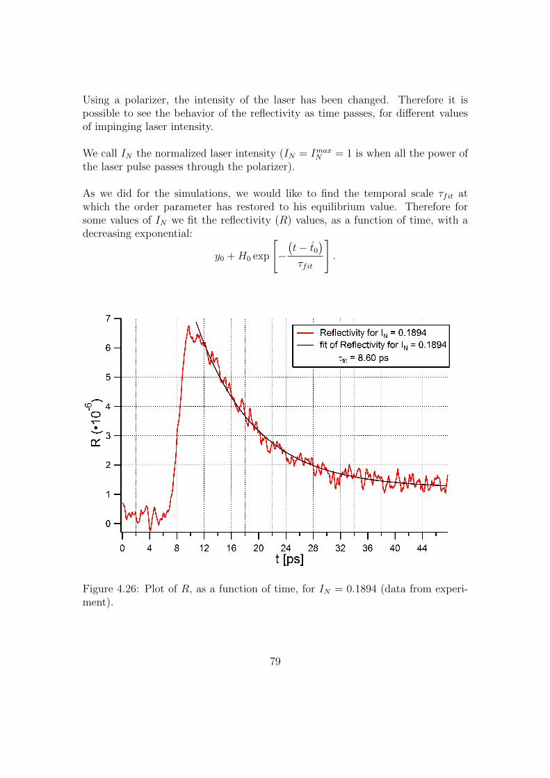
Using a polarizer, the intensity of the laser has been changed. Therefore it ispossible to see the behavior of the reflectivity as time passes, for different valuesof impinging laser intensity.
We call IN the normalized laser intensity (IN = ImaxN = 1 is when all the power ofthe laser pulse passes through the polarizer).
As we did for the simulations, we would like to find the temporal scale τfit atwhich the order parameter has restored to his equilibrium value. Therefore forsome values of IN we fit the reflectivity (R) values, as a function of time, with adecreasing exponential:
y0 +H0 exp
[−(t− t0
)τfit
].
Figure 4.26: Plot of R, as a function of time, for IN = 0.1894 (data from experi-ment).
79
For all the analyzed laser intensities we obtained τfit ∼ 8 ps.
Now we would like to analyze the system at short times after the laser pulse, i.e.where the effect of the perturbation is large.
• We choose to analyze the reflectivity of the system, as a function of the laserintensity, after 25 % of τfit (i.e. after 2 ps, for the analyzed case) from thelaser pulse switching off.
• For each studied IN we average the reflectivity from 13.30 ps to 13.31 ps,because the laser switching off was at the moment t0 ∼ 11 ps on the usedtemporal scale (see figure 4.26).
• We note that the average over a short time interval (100 fs) could be affectedby noise. To avoid this problem, we make also a second analysis, averagingon a larger time interval: for each studied IN we average the reflectivity from10 ps to 13 ps.
• We normalize the value of reflectivity, dividing it by its maximum value. Sowe obtain the normalized average reflectivity < R >, see markers in figure4.27.
• We would like to compare the experimental < R > with |< δη >| fromsimulations. Therefore we analyze |< δη >| after 0.5 s (25 % of τfit), seeblue line in figure 4.27.
80

Figure 4.27: Blue continuous line: plot of |< δη >| as a function of the laserintensity I for t = 0.5 s (values from simulations). Red markers: plot of < R > asa function of the normalized laser intensity IN (average made from 10 ps to 13 ps).Green markers: plot of < R > as a function of the normalized laser intensity IN(average made from 13.30 ps to 13.31 ps).
From this figure we note that in both cases < R > has the same functionalbehavior of |< δη >|. However < R > reaches the saturation for IN = 1, while|< δη >| saturates for I = 250.
Actually I and IN have not the same meaning, because we do not know whichphysical situation correspond to a certain IN . Therefore we would like to find therelation between I and IN .
IN = 1 means that the sample is excited by the maximum laser intensity availablefrom the used experimental setup. Evidently a region of the sample has beenbrought in the state with η = 0.
Comparing < R > graph and |< δη >| graph2, we would like to define the region
2We assume that relation (4.3) holds. Since we are dealing with a normalized reflectivity, wecan deduce γ = 1 in this case.
81
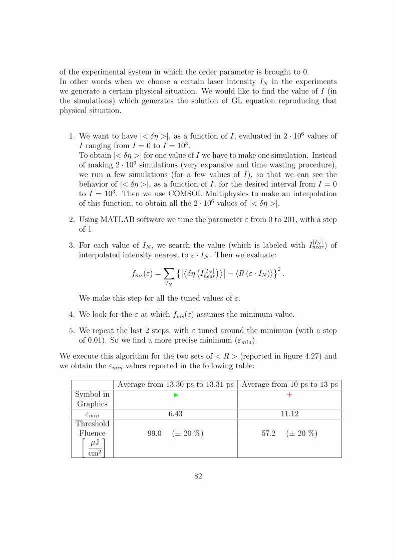
of the experimental system in which the order parameter is brought to 0.In other words when we choose a certain laser intensity IN in the experimentswe generate a certain physical situation. We would like to find the value of I (inthe simulations) which generates the solution of GL equation reproducing thatphysical situation.
1. We want to have |< δη >|, as a function of I, evaluated in 2 · 106 values ofI ranging from I = 0 to I = 103.To obtain |< δη >| for one value of I we have to make one simulation. Insteadof making 2 · 106 simulations (very expansive and time wasting procedure),we run a few simulations (for a few values of I), so that we can see thebehavior of |< δη >|, as a function of I, for the desired interval from I = 0to I = 103. Then we use COMSOL Multiphysics to make an interpolationof this function, to obtain all the 2 · 106 values of |< δη >|.
2. Using MATLAB software we tune the parameter ε from 0 to 201, with a stepof 1.
3. For each value of IN , we search the value (which is labeled with I[IN ]near) of
interpolated intensity nearest to ε · IN . Then we evaluate:
fms(ε) =∑IN
∣∣⟨δη (I [IN ]near
)⟩∣∣− 〈R (ε · IN)〉2.
We make this step for all the tuned values of ε.
4. We look for the ε at which fms(ε) assumes the minimum value.
5. We repeat the last 2 steps, with ε tuned around the minimum (with a stepof 0.01). So we find a more precise minimum (εmin).
We execute this algorithm for the two sets of < R > (reported in figure 4.27) andwe obtain the εmin values reported in the following table:
Average from 13.30 ps to 13.31 ps Average from 10 ps to 13 psSymbol in I +Graphicsεmin 6.43 11.12
ThresholdFluence 99.0 (± 20 %) 57.2 (± 20 %)[
µJ
cm2
]
82
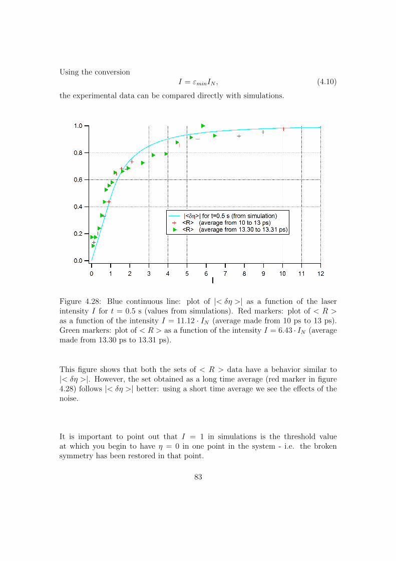
Using the conversionI = εminIN , (4.10)
the experimental data can be compared directly with simulations.
Figure 4.28: Blue continuous line: plot of |< δη >| as a function of the laserintensity I for t = 0.5 s (values from simulations). Red markers: plot of < R >as a function of the intensity I = 11.12 · IN (average made from 10 ps to 13 ps).Green markers: plot of < R > as a function of the intensity I = 6.43 · IN (averagemade from 13.30 ps to 13.31 ps).
This figure shows that both the sets of < R > data have a behavior similar to|< δη >|. However, the set obtained as a long time average (red marker in figure4.28) follows |< δη >| better: using a short time average we see the effects of thenoise.
It is important to point out that I = 1 in simulations is the threshold valueat which you begin to have η = 0 in one point in the system - i.e. the brokensymmetry has been restored in that point.
83

In the case of a superconductor, for instance, the system is brought in normalstate in the region where η = 0.Therefore, from the conversion relation (4.10), we can say that the threshold laserintensity is I thN = 1/εmin.
Reminding that IN is normalized, we have the following relation:
I thNImaxN
= I thN =1
εmin.
So the power to apply in order to have the threshold situation is:
Threshold Power =Threshold Power
Maximum Power·Maximum Power =
=I thNImaxN
·Maximum Power =1
εmin·Maximum Power =
1
εmin· 8 mW
and therefore the energy per pulse to have the threshold situation is:
1
εmin· Maximum Power
Repetition Rate=
1
εmin· 8 mW
250 kHz.
Finally we can introduce the fluence to have the threshold situation as the corre-sponding energy per pulse divided by the laser spot area:
Threshold F luence =1
εmin· Maximum Power
π(Spot Diameter
2
)2 ·Repetition Rate =
=1
εmin· 8 mW
π(80 µm
2
)2 · 250 kHz.
The obtained threshold fluence values are reported in the last table.The error for the threshold fluence is due to the propagation of the spot diametererror.
The obtained threshold fluence values can be compared with the experimental one(ΦC), estimated as the value at which there is the transition from a low excitationregime (when the fluence is small and < R > increases proportionally to thefluence) to a high excitation regime (when the fluence is high and < R > has asub-linear dependence on the fluence).The threshold fluence values obtained from simulations have the same order ofmagnitude of the experimental fluence (estimated as ΦC = 26 µJ/cm2). Howeverdue to the big error on the spot diameter, the values obtained from simulationsare not very precise.
84
4.2 Technical details
To obtain the data in Chapter 4 we use a “2D-Axisymmetric Model”, with a“Coefficient Form PDE” physics.Then we introduce the model parameters. Since in COMSOL Multiphysics wecannot use Greek letters as parameters, we use:
Parameter names in COMSOL Multiphysics Corresponding parameter in our workomega ωalpha αlambda λ
A AB B
penetrazione lpenlarghezza lwidth
I I
The parameters used for each simulation are specified near the reported results.
Geometry:
• The geometry used is a rectangle 2 m× 0.3 m, built in the (r, z) plain (withreference to figure 4.7).
If I > 1, the geometry is more complicate:
• We create a parametric curve to define the parabola introduced in equation(4.4). The dimensionless parameter s, defining the parametric curve, hasto represent the variable r in equation (4.4). So we assign the followingexpression to r coordinate in the “Expressions” field:
s ∗ 1 [m].
To obtain the parabola, the parameter s ranges from 0 to
larghezza ∗ sqrt(log(I))/1 [m].
In COMSOL Multiphysics “log” stands for natural logarithm and “sqrt”stands for square root.
85
Then we write the following expression for z coordinate in the “Expressions”field:
(−s2 ∗ 1[m2]/larghezza2 + log(I)) ∗ penetrazione.
So we obtain a parabola.
Finally, in “Position” field we set r = 0 and z = 0. We write 0 in the“Rotation Angle” field.
• We create a segment:from (r = 0, z = 0) to (r = larghezza ∗ sqrt[log(I)], z = 0)and a segment:(r = 0, z = 0) to (r = 0, z = log(I) ∗ penetrazione).
To create a segment we right-click over the voice “Geometry” and we choose“Bezier Poligon”. Then we choose “Open curve” in the “Type” field, andclick on “Add linear”. So we can introduce the coordinates of the segmentbeginning and end.
• We right-click on “Geometry”, we choose “Boolean operation→ Union”, weselect the parabola and the 2 segments to make the union (we select “Keepinterior boundaries”).The “Union” of the parabola and the 2 segments generates a closed curve.
• We right-click on “Geometry”, we choose “Conversions→ Convert to Solid”,we select the closed curve obtained from the “Union” in the last step, to makean irregular plane figure, surrounded by that closed curve.
• We right-click on “Geometry”, we choose “Boolean operation→ Difference”,we select the rectangle as “Object to add” and the irregular plane figuregenerated in the last step as “Object to subtract” to create the “domain 2”(we select “Keep interior boundaries” and “Keep input objects”).
• We right-click on “Geometry”, we choose “Boolean operation → Intersec-tion”, we select the rectangle and the irregular plane figure generated in theprevious steps to create the “domain 1” (we select “Keep interior bound-aries”).“domain 1” and “domain 2” are drawn in figure 4.29.
• If penetrazione < 0.3 m we create a segment:from (r = 0, z = 0) to (r = 0, z = penetrazione),over which the solution will be averaged. If penetrazione < 0.3 m, we do
86
not need to create this segment, because the average will be made on theboundary of the rectangle.
Clicking on “Coefficient Form PDE” we choose “Dimensionless” as “Dependentvariable quantity” (u), “None” for the “Source term quantity” field and 1 for the“Unit” field.Then we introduce the coefficient in the “Coefficient Form PDE”; referring toequation (2.1):
ea∂2u
∂t2+ da
∂u
∂t+∇ · (−c∇u−αu+ γ) + β · ∇u+ au = f, (2.1)
we assign the following coefficients:
Terms in equation (2.1) Assigned coefficientsc lambda (Isotropic)a Af −B ∗ u3ea 1/omega2
da alpha/omegaα (0, 0)β (0, 0)γ (0, 0)
As boundary conditions we apply “Zero Flux” boundary condition to all externalboundaries (see next figure).
COMSOL Multiphysics applies automatically continuity of the solution u and ofc∇u at the internal boundaries, since we do not assign them an explicit condition.
87
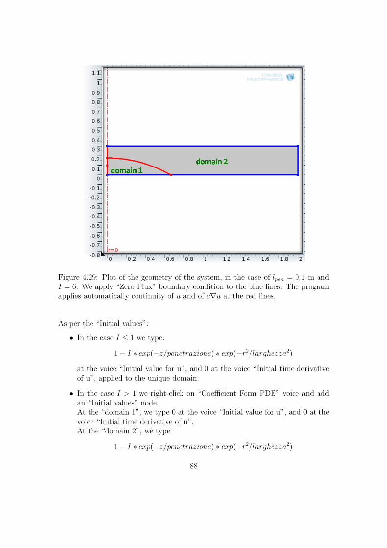
Figure 4.29: Plot of the geometry of the system, in the case of lpen = 0.1 m andI = 6. We apply “Zero Flux” boundary condition to the blue lines. The programapplies automatically continuity of u and of c∇u at the red lines.
As per the “Initial values”:
• In the case I ≤ 1 we type:
1− I ∗ exp(−z/penetrazione) ∗ exp(−r2/larghezza2)
at the voice “Initial value for u”, and 0 at the voice “Initial time derivativeof u”, applied to the unique domain.
• In the case I > 1 we right-click on “Coefficient Form PDE” voice and addan “Initial values” node.At the “domain 1”, we type 0 at the voice “Initial value for u”, and 0 at thevoice “Initial time derivative of u”.At the “domain 2”, we type
1− I ∗ exp(−z/penetrazione) ∗ exp(−r2/larghezza2)
88

at the voice “Initial value for u”, and 0 at the voice “Initial time derivativeof u”.
As per the Mesh we choose a “Physics-controlled mesh”, with “Extremely fine”element size (that is to say a triangular Mesh with 0.02 m as “Maximum elementsize”).
We use a “Time Dependent Study”, with “Generalized alpha” time steppingmethod. The steps taken by solver are manual, with a time step of 10−2.
When the numerical solution is obtained we make an average, right clicking on“Derived Values” node and choosing “Average → Line Average”. Then under thevoice “Line Average” we select the domains over which we want to average.
89

References
1. G. Coslovich, C. Giannetti, F. Cilento, S. Dal Conte, G. Ferrini, P. Galinetto,M. Greven, H. Eisaki, M. Raichle, R. Liang, A. Damascelli, F. Parmi-giani, Evidence for a photoinduced nonthermal superconducting-to-normal-state phase transition in overdoped Bi2Sr2Ca0.92Y0.08Cu2O8+δ, PHYSICALREVIEW B 83, 064519 (2011).
2. Claudio Giannetti, Giacomo Coslovich, Federico Cilento, Gabriele Ferrini,Hiroshi Eisaki, Nobuhisa Kaneko, Martin Greven, Fulvio Parmigiani, Dis-continuity of the ultrafast electronic response of underdoped superconductingBi2Sr2CaCu2O8+δ strongly excited by ultrashort light pulses, PHYSICAL RE-VIEW B 79, 224502 (2009).
3. Claudio Giannetti, Federico Cilento, Sstefano Dal Conte, Giacomo Coslovich,Gabriele Ferrini, Hajo Mmolegraaf, Mmarkus Raichle, Ruixing Liang, Hi-roshi Eisaki, Mmartin Greven, Andrea Damascelli, Dirk van der Mmarel,Fulvio Parmigiani, Revealing the high-energy electronic excitations underly-ing the onset of high-temperature superconductivity in cuprates, Nature Com-munications (2011).
90

Chapter 5
Super-lattice composed bymaterials with broken symmetry
In this brief chapter we would like to expose some possible applications of ourwork.It is worth to introduce a super-lattice, characterized by a periodic unit cellcomposed by layers of different materials. In our analysis, the chosen materialssupport a real order parameter, satisfying GL equation (1.13).Therefore this theory applies to all materials with a broken symmetry, inparticular superconductors or ferromagnetic materials.
We would like to analyze how a perturbation of the order parameter propagatesthrough the super-lattice. For this purpose we choose materials with low damping(α << 1). Therefore GL equation reduces to:
1
ω2
∂2η
∂t2− λ∇2η + A(P, T )η +B(P )η3 = 0. (5.1)
Equation (5.1) has the form of a wave equation (the first 2 terms) with a sourceterm (the last 2 terms).For sake of simplicity, we work with a 1D super-lattice, with a unit cell character-ized by 2 layers of different material.
The general solution of equation (5.1) can be written using the Fourier transform:
η(x, t) =
∫ +∞
−∞
∫ +∞
−∞η(k, ω) eikx eiωt dk dω.
Considering that the equation (5.1) should be solved for the super-lattice geometry,ω must be related to k by a dispersion relation:
ω = f(k).
91
Our target is to work out the dispersion relation, very useful to predict how awave packet propagates through the super-lattice.
The dispersion relation can predict if a certain frequency cannot pass through thesuper-lattice, if there are no k values allowed for that frequency. The dispersionrelation can show if there are frequency gaps, i.e. zones in the frequency spectrumwhose frequencies does not pass through the super-lattice.
The dispersion relation can predict the velocity of propagation of a certainfrequency in the super-lattice.
Actually the dispersion relation should depend on the choice of the materialsand on the geometry of the built unit cell. With an opportune choice of thematerials composing the super-lattice or of the unit cell geometry, we can modifythe dispersion relation.
A possible application is the creation of a frequencies filter: with an opportunechoice of the materials we can control the frequency gaps of the super-latticeso that only certain desired frequencies in a wave packet can pass through thesuper-lattice.
There are different possibilities to simulate this physical situation. In our work wetreat:
1. A “many unit cells geometry”: the super-lattice is approximated by repeatinga lot of times the unit cell. So we see the behavior of a finite super-lattice,but if we repeat the unit cell for a high number of times the final solutionwill be a good approximation to the theoretical infinite super-lattice.
2. A “one unit cell geometry”: we analyze the behavior of a single unit cell. Toreproduce the infinite super-lattice behavior we apply a periodic boundarycondition.
92

5.1 Many unit cells geometry
We build a super-lattice composed by 6 unit cells. Each unit cell is composed bytwo layers of two different materials (called “Material 1” and “Material 2”).We suppose that the two used materials satisfy the GL equation (5.1), and thatthey have the same coefficients ω, λ, B, but A coefficient can be different.The super-lattice is put between 2 slices, an initial layer and a detector layer,made of “Material 1”, see figure 5.1.
Figure 5.1: The super-lattice. The black segments represent the “Material 1”, theorange segments represent the “Material 2”. The used system of coordinate isindicated.
In this section we would like to see how a wave packet propagates through thesuper-lattice. This wave packet is produced by perturbing the order parameterwith a laser pulse (switching off at time t = 0 s), at the beginning of the system(x = 0).Since we want to analyze how the pulse passes through the super-lattice, weimpose zero-flux boundary condition at the external boundaries, so the systemis isolated from the external world and we are sure that all the perturbationis driven towards the super-lattice. From one layer to another we impose thecontinuity of the solution and of the first spatial derivative of the solution.
We use COMSOL Multiphysics to obtain a numerical solution of equation (5.1).First we seek the equilibrium solution ηeq solving equation (5.1) with a “stationarystudy”.Next we would like to solve the equation (5.1) in the time domain. To simulatethe laser pulse we choose the following expressions as initial values:
η(x, t = 0 s) = ηeq [1− I exp(−x/lpen)] , (5.2)
dη
dt
∣∣∣∣t=0
= 0 s−1,
applied to all the domains.
93
Therefore at the initial time there is a wave packet before the super-lattice(decreasing exponential perturbation of the equilibrium order parameter). Thispacket will evolve and we would like to see if the perturbation passes thesuper-lattice.
We compute simulations keeping fixed the following parameters:
• ω = 0.1 s−1;
• λ = 0.18 m2;
• lpen = 1 m;
• B = 1 (dimensionless).
In “Material 1” we fix A = −1, while in “Material 2” we use different values ofA (for simplicity we use the notation A2 to mean the coefficient A used in the“Material 2”), so that we can have a low or a high contrast between the twomaterials.
As for the geometry, we choose a unit cell composed by a 4 m layer of “Material2” and a 4 m layer of “Material 1”. Then we use a 4 m initial layer and a 20 mdetector layer.
We make a simulation with A2 = −0.9, i.e. the difference between the two ma-terials is little. The results are exposed in figure 5.2, in which you can see theorder parameter behavior (color scale) in the super-lattice geometry (horizontalaxis) and in time (vertical axis).
94

Figure 5.2: The evolution of the order parameter (color scale) in the geometry, asa function of time, for A2 = −0.9.
Then we make another simulation in which A2 = −0.1, i.e. the difference betweenthe 2 materials is important. The results are exposed in figure 5.3,
Figure 5.3: The evolution of the order parameter (color scale) in the geometry, asa function of time, for A2 = −0.1.
95

As you can see, in the initial layer the order parameter oscillates in time, inagreement with the fact that we are dealing with an undamped system.
You can also see that the order parameter passes through the super-lattice, arrivingin the detector layer. However in the detector layer the perturbation intensity islower, because the wave packet spreads during the travel through the super-lattice.
96
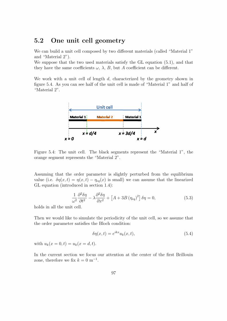
5.2 One unit cell geometry
We can build a unit cell composed by two different materials (called “Material 1”and “Material 2”).We suppose that the two used materials satisfy the GL equation (5.1), and thatthey have the same coefficients ω, λ, B, but A coefficient can be different.
We work with a unit cell of length d, characterized by the geometry shown infigure 5.4. As you can see half of the unit cell is made of “Material 1” and half of“Material 2”.
Figure 5.4: The unit cell. The black segments represent the “Material 1”, theorange segment represents the “Material 2”.
Assuming that the order parameter is slightly perturbed from the equilibriumvalue (i.e. δη(x, t) = η(x, t) − ηeq(x) is small) we can assume that the linearizedGL equation (introduced in section 1.4):
1
ω2
∂2δη
∂t2− λ∂
2δη
∂x2+[A+ 3B (ηeq)
2] δη = 0, (5.3)
holds in all the unit cell.
Then we would like to simulate the periodicity of the unit cell, so we assume thatthe order parameter satisfies the Bloch condition:
δη(x, t) = eikxuk(x, t), (5.4)
with uk(x = 0, t) = uk(x = d, t).
In the current section we focus our attention at the center of the first Brillouinzone, therefore we fix k = 0 m−1.
97
Therefore we make the substitution δη(x, t) = u0(x, t) in equation (5.3) to obtain:
1
ω2
∂2u0∂t2− λ∂
2u0∂x2
+[A+ 3B (ηeq)
2]u0 = 0. (5.5)
For both materials we choose the following parameters:
• ω = 0.1 s−1;
• λ = 0.18 m2;
• B = 1 (dimensionless).
In “Material 1” we fix A = −1.
For simplicity we use the notation A2 to mean the coefficient A used in the“Material 2”. We make some simulations changing the value of A2 (i.e. changingthe contrast between the 2 used materials).
As for the geometry, we choose a unit cell with length d = 8 m.
For each value of A2, we make a simulation using COMSOL Multiphysics. Inparticular we solve the equilibrium equation (1.10) for a real order parameter nu-merically, with a “Stationary Study”, to evaluate ηeq; then we use the equilibriumvalue found to look for the first 10 eigenvalues of equation (5.5).
In figure 5.5 we report the relative distance between the second and the thirdeigenvalue (∆ωeig), as a function of the value of A2 coefficient.
As you can see, when the unit cell is composed by an homogeneous material(A2 = −1) the second and the third eigenvalue are degenerate.
When A2 increases, the contrast between the 2 used materials grows. The secondand the third eigenvalue split and so we can understand that there is a gap in thefrequency spectrum. The more the “Material 2” is different from the “Material1” (the more A2 grows in our simulations), the more the frequency gap increases.
It is also interesting to point out that the gap value is appreciable, because it isup to 15% of the eigenvalue values.
98
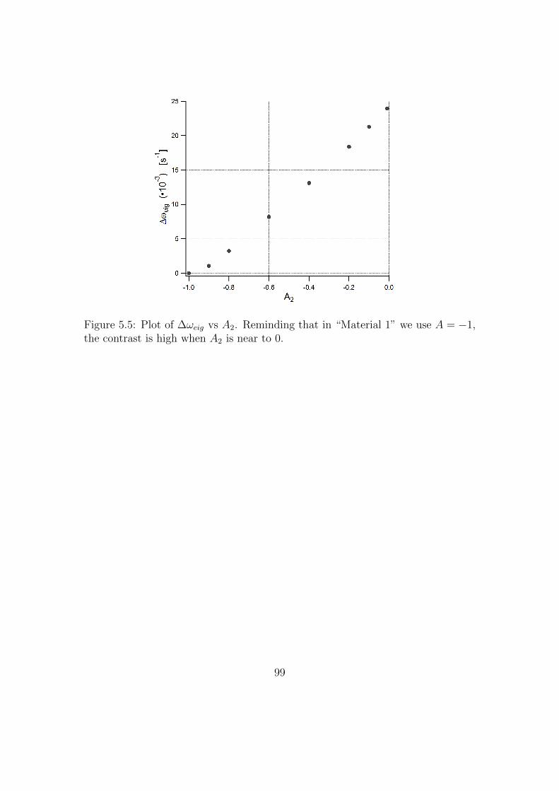
Figure 5.5: Plot of ∆ωeig vs A2. Reminding that in “Material 1” we use A = −1,the contrast is high when A2 is near to 0.
99
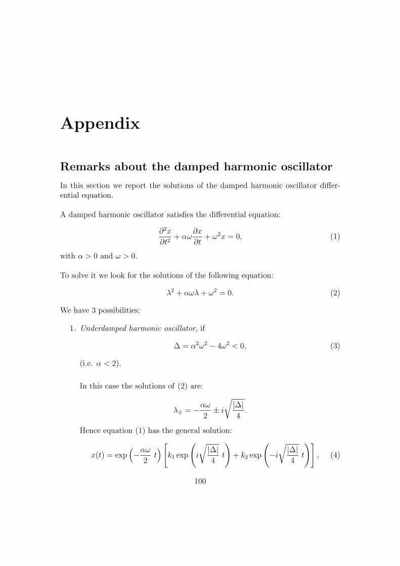
Appendix
Remarks about the damped harmonic oscillator
In this section we report the solutions of the damped harmonic oscillator differ-ential equation.
A damped harmonic oscillator satisfies the differential equation:
∂2x
∂t2+ αω
∂x
∂t+ ω2x = 0, (1)
with α > 0 and ω > 0.
To solve it we look for the solutions of the following equation:
λ2 + αωλ+ ω2 = 0. (2)
We have 3 possibilities:
1. Underdamped harmonic oscillator, if
∆ = α2ω2 − 4ω2 < 0, (3)
(i.e. α < 2).
In this case the solutions of (2) are:
λ± = −αω2± i√|∆|4.
Hence equation (1) has the general solution:
x(t) = exp(−αω
2t)[
k1 exp
(i
√|∆|4
t
)+ k2 exp
(−i√|∆|4
t
)], (4)
100
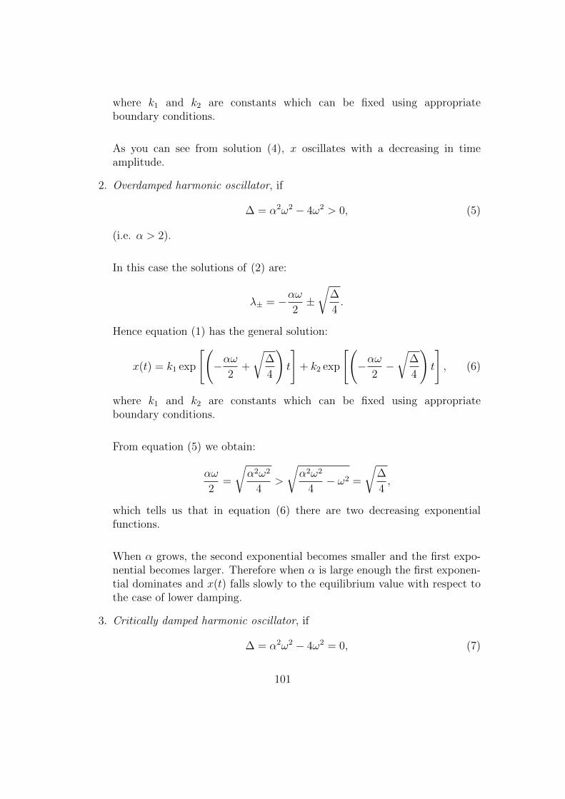
where k1 and k2 are constants which can be fixed using appropriateboundary conditions.
As you can see from solution (4), x oscillates with a decreasing in timeamplitude.
2. Overdamped harmonic oscillator, if
∆ = α2ω2 − 4ω2 > 0, (5)
(i.e. α > 2).
In this case the solutions of (2) are:
λ± = −αω2±√
∆
4.
Hence equation (1) has the general solution:
x(t) = k1 exp
[(−αω
2+
√∆
4
)t
]+ k2 exp
[(−αω
2−√
∆
4
)t
], (6)
where k1 and k2 are constants which can be fixed using appropriateboundary conditions.
From equation (5) we obtain:
αω
2=
√α2ω2
4>
√α2ω2
4− ω2 =
√∆
4,
which tells us that in equation (6) there are two decreasing exponentialfunctions.
When α grows, the second exponential becomes smaller and the first expo-nential becomes larger. Therefore when α is large enough the first exponen-tial dominates and x(t) falls slowly to the equilibrium value with respect tothe case of lower damping.
3. Critically damped harmonic oscillator, if
∆ = α2ω2 − 4ω2 = 0, (7)
101
(i.e. α = 2).
In this case the solutions of (2) are degenerate:
λ± = −αω2.
Hence equation (1) has the general solution:
x(t) = k1 exp(−αω
2t)
+ k2 t exp(−αω
2t), (8)
where k1 and k2 are constants which can be fixed using appropriateboundary conditions.
102