Embed Size (px)
Citation preview
iq ·-;.*"~- ' .. .
. ,.A R .,,,
DIGITAL CONTROL OF GYROSCOPE DRIFT COMPENSATION
by
Donald W. Fleischer
B. E. E., Union College
1956
SUBMITTED IN PARTIAL FULFILLMENT OF THE
REQUIREMENTS FOR THE DEGREE OF
MASTER OF SCIENCE
at the
MASSACHUSETTS INSTITUTE OF TECHNOLOGY
June, 1961
Signature of Author _
Department of Electrical Engineering, May 20, 1961
Certified byThesis Supervisor
Accepted by , / ..-Chairman, Deptmrnental Coomittee on Graduit-Students
1

0C�
DIGITAL CONTROL OF GYROSCOPE DRIFT COMPENSATION
by
Donald W. Fleischer
Submitted to the Department of Electrical Engineering onMay 20, 1961 in partial fulfillment of the requirements for thedegree of Master of Science.
ABSTRACT
This thesis is concerned with the use of digital signals forthe control of gyroscope drift compensation. Several possiblemethods for digitally controlling the torque produced by a gyroscopetorque generator are presented with block diagrams of the hardwarerequired. Possible sources of error introduced by the use of thesemethods are analyzed. Tests that were conducted using the torquecontrol methods presented are described. The results indicate thatdigitally controlled gyroscope drift compensation is quite feasibleif certain requirements are followed.
Thesis Supervisor: Richard H. Frazier
Title: Associate Professor ofElectrical Engineering
iIR
V T
3

j .v
ACKNOWLEDGEMENT
The author is grateful to Professor Richard Frazier for his
supervision and assistance in acting as thesis adviser.
The author wishes to thank those personnel of the M. I. T.
Instrumentation Laboratory who assisted with their comments and
especially Harry Margulius who worked with the author during
many of the tests.
The author also wishes to thank his wife for her efforts and
patience in typing this thesis.
This report was prepared under Project 52-154, Division of
Sponsored Research, Massachusetts Institute of Technology,
sponsored by the Navigation and Guidance Laboratory of the Wright
Air Development Division, Department of the Air Force, under
Contract AF33(600) - 38967.
The publication of this report does not constitute approval by the
U. S. Air Force, or the Instrumentation Laboratory of the findings
or the conclusions contained therein. It is published only for the
exchange and stimulation of ideas.
5

C
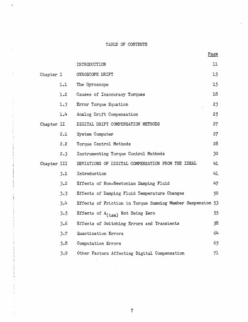
TABLE OF CONTENTS
Chapter I
1.1
1.2
1.3
1.4
Chapter II
2.1
2.2
2.3
Chapter III
3.1
3.2
3.3
3.4
3.5
3.6
3-7
3.8
3.9
Page
INTRODUCTION 11
GYROSCOPE DRIFT 15
The Gyroscope 15
Causes of Inaccuracy Torques 18
Error Torque Equation 23
Analog Drift Compensation 25
DIGITAL DRIFT COMPENSATION METHODS 27
System Computer 27
Torque Control Methods 28
Instrumenting Torque Control Methods 30
DEVIATIONS OF DIGITAL COMPENSATION FROM THE IDEAL 41
Introduction 41
Effects of Non-Newtonian Damping Fluid 47
Effects of Damping Fluid Temperature Changes 50
Effects of Friction in Torque Summing Member Suspension 53
Effects of A(tsm) Not Being Zero 55
Effects of Switching Errors and Transients 58
Quantization Errors 64
Computation Errors 65
Other Factors Affecting Digital Compensation 71
7
TABLE OF CONTENTS (continued)
Chapter IV
4.1
4.2
4.3
Chapter V
5.1
5.2
5.3
Bibliographjr
DIGITAL COMPENSATION TESTS
Introduction
Test Methods
Tests and Results
CONCLUSIONS
Discussion of Test Results
Conclusions
Recommendations for Further Study
8
7'3
73
77
78
87
87
9o0
92
93
LIST OF FIGURES
Figure Page
1-1 Line Schematic Diagram of Gyroscope 16
1-2 Diagram Showing How Unequal Compliances Can CauseInaccuracy Torques 21
2-1 Block Diagram of Torque Control Method #1 31
2-2 Block Diagram of Torque Control Method #2 33
2-3 Block Diagram of Countdown Register 34
2-4 Ideal Current Waveforms for Zero Torque Output Using
Torque Control Method #2 36
2-5 Block Diagram of Torque Control Method #3 37
2-6 Block Diagram of Torque Control Method #4 40
3-1 Simplified Block Diagram of Single-Axis GyroscopeStabilization Drive 43
3-2 Typical Torque Acting On Torque Summing Member 46
3-3 Ideal Viscosity Changes of Test Gyroscope Damping Fluid 52
3-4 Torque Generator Input Current Waveforms Showing TransientsCaused by Switching 60
3-5 Computed Error Torque Quantization 69
4-1 Block Diagram of Test Setup 74
4-2 Schematic Diagram of Electronic Switch 76
9

lo
INTRODUCTION
With the advent of the replacement of analog computers by
special purpose digital computers in inertial navigation systems,
certain changes in the system instrumentation have become necessary.
One of these required changes is in the method used to compensate
for gyroscope drift. Basically, the problem is one of using sampled
data to perform a function where continuous signals were previously
available.
Gyroscope drift is caused by unwanted torques which act on the
gyroscope torque summing member about the output axis. These unwanted
torques result from inaccuracies in the manufacture of the gyroscope
and from certain causes inherent in its design. Ideally, a drift
compensation system applies a torque to the gyroscope float which
occurs simultaneously with and is equal in magnitude and opposite in
direction to the unwanted torques, thus completely cancelling them.
Some of the unwanted torques are functions of gravity and the
acceleration of the vehicle in which the inertial navigation system
is contained. When a gyroscope is mounted in an inertial system, there
is no way of distinguishing between these torques and the desired
precession torques. Therefore, before the gyroscope is mounted in the
system, the magnitudes and directions of the unwanted torques must be
determined for conditions of gravity and acceleration which the
vehicle will encounter. One of the functions of the inertial system
computer is to take this previously determined information and
II
calculate, for existing conditions, what the unwanted torques are and
hence what the compensating torques should be.
When an analog computer is used for this function, continuous
torque information is produced. In this form, the information is
ideally suited to controlling compensating torques, since the unwanted
torques are continuous quantities. Thus a compensation system em-
ploying analog computation is theoretically capable of producing
ideal compensation.
Digital computers, due to their nature, produce discontinuous
output information. Therefore a compensation system employing digital
computation, even under ideal conditions, cannot achieve ideal com-
pensation. This means that unwanted torques act on the gyroscope
float causing small angular movements. These movements can be the
source of certain errors. This thesis investigates some possible
digital compensation methods and attempts to analyze the errors
introduced by them.
The first chapter briefly reviews the causes of gyroscope drift.
It gives the equation that describes the unwanted torques causing the
drift and tells how the constants are obtained. Gyroscope torque
generator operation and analog drift compensation are also outlined.
Chapter II gives descriptions of several possible methods of
instrumenting a digital compensation system. It lists the advantages
and disadvantages of each method.
Chapter III analyzes the errors introduced by the compensation
methods of Chapter II.
12
The fourth chapter describes tests that were made on a gyroscope
to determine the actual errors introduced by digital controlled com-
pensation. A description is given of the equipment used and the
results are presented.
The last chapter briefly analyzes the results of Chapter IV.
Some conclusions are drawn and a short summary given.
13

1'
Chapter I
GYROSCOPE DRIFT
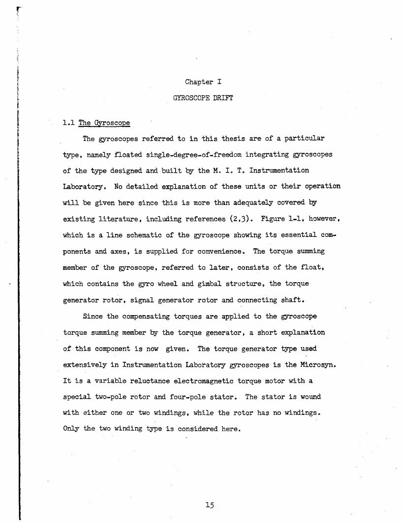
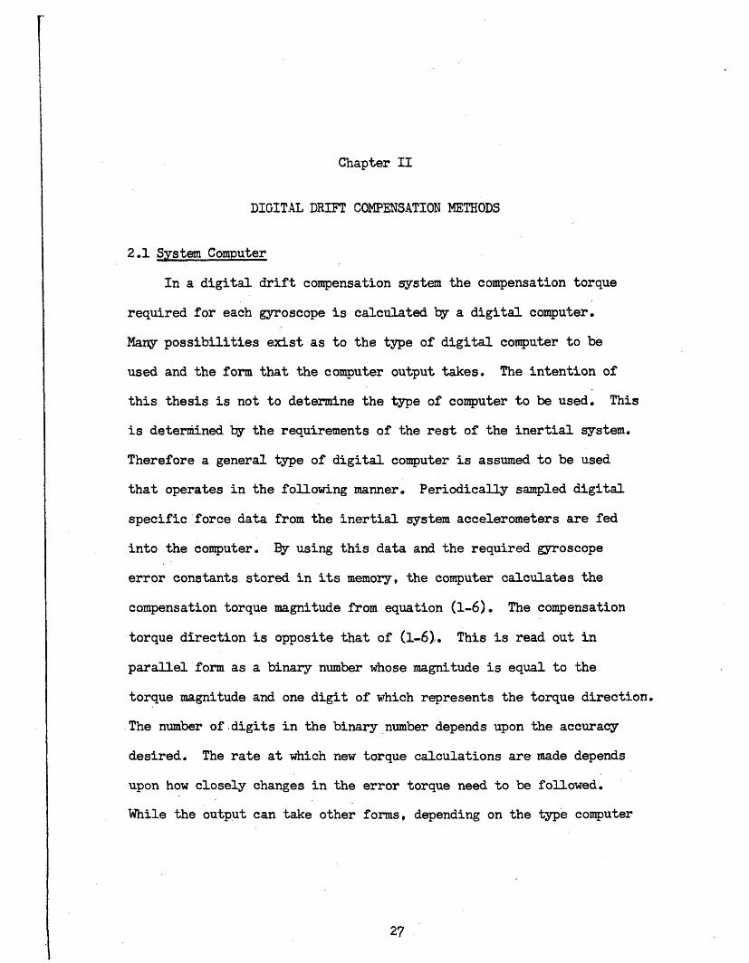
1.1 The Gyroscope
The gyroscopes referred to in this thesis are of a particular
type, namely floated single-degree-of-freedom integrating gyroscopes
of the type designed and built by the M. I T Instrumentation
Laboratory. No detailed explanation of these units or their operation
will be given here since this is more than adequately covered by
existing literature, including references (2,3). Figure 1-1, however,
which is a line schematic of the gyroscope showing its essential com-
ponents and axes, is supplied for convenience. The torque summing
member of the gyroscope, referred to later, consists of the float,
which contains the gyro wheel and gimbal structure, the torque
generator rotor, signal generator rotor and connecting shaft.
Since the compensating torques are applied to the gyroscope
torque summing member by the torque generator, a short explanation
of this component is now given. The torque generator type used
extensively in Instrumentation Laboratory gyroscopes is the Microsyn.
It is a variable reluctance electromagnetic torque motor with a
special two-pole rotor and four-pole stator The stator is wound
with either one or two windings, while the rotor has no windings.
Only the two winding type is considered here.
15
SignalGenerator
TorqueGenerator
Gimbal
GyroWheel
- \ O utputAxis
;pin ReferenceAxis
:is A(tsm)
InputAxis
Figure 1-1 Line Schematic Diagramof Gyroscope
16
Beari n
itTruV
r
;
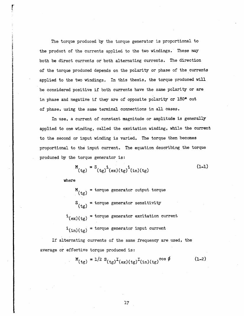
The torque produced by the torque generator is proportional to
the product of the currents applied to the two windings. These may
both be direct currents or both alternating currents. The direction
of the torque produced depends on the polarity or phase of the currents
applied to the two windings. In this thesis, the torque produced will
be considered positive if both currents have the same polarity or are
in phase and negative if they are of opposite polarity or 180° out
of phase, using the same terminal connections in all cases.
In use, a current of constant magnitude or amplitude is generally
applied to one winding, called the excitation winding, while the current
to the second or input winding is varied. The torque then becomes
proportional to the input current. The equation describing the torque
produced by the torque generator is:
M(tg) (tg) (ex)(tg) (in)(tg) (1-1)
where
M(tg) = torque generator output torque
S(tg) = torque generator sensitivity
i(ex)(tg)-= torque generator excitation current
i(in)(tg) = torque generator input current
If alternating currents of the same frequency are used, the
average or effective torque produced is:
N 1/2 S- I cos.(1-2)M(tg) = 1/2 S(tg) I(ex)(tg) (in)(tg)C)
17
where
I(ex)(tg) and (in)(tg ) = the amplitudes of the
torque generator currents
0 = phase angle between the two
currents.
Therefore when the two currents are 90° out of phase the effective
torque produced is zero. The torque is independent of frequency over
a specified operating range. In this thesis, any torques referred to
will be effective torques, unless otherwise specified.
1.2 Causes of Inaccuracy Torques
Essentially there are four types of torques that operate on the
gyroscope torque summing member. They are: .(a) the gyro wheel
precessional torque caused by an angular velocity of the gyroscope
case with respect to inertial space about the input axis; (b) the
viscous damping torque; (c) desired torques produced by the torque
generator and (d) inaccuracy torques. The first three are considered
to be perfect torques. In actual operation the torques usually
grouped under these headings are not perfect. However, here they
each are considered to be separated into perfect and imperfect parts,
the latter parts all being included with the inaccuracy torques. If
the inaccuracy torques, also referred to as unbalance torques or
drift torques, were not present, the gyroscope would perform perfectly.
The inaccuracy torques can be further divided into error torques
and uncertainty torques. Error torques are by definition predictable
18
and therefore can be compensated. Uncertainty torques are unpredictable
and hence cannot be compensated. Assuming the error torques can be
perfectly predicted and compensated, the ultimate gyroscope performance
limit is determined by the magnitude of the uncertainty torques.
Inaccuracy torques are caused by several factors. The significant
ones are listed below. The following abbreviations are used during
this discussion:
S. R. A. = spin reference axis
I. A. = input axis
O A = output axis
(a) Fixed unbalance or endulous torques, caused by the center
of mass of the torque summing member not lying exactly on the gyro-
scope output axis. For analysis, the unbalance is separated into two
components, one assumed fixed along the positive S. R. A., U(SRA) , and
one assumed fixed along the positive I. A., U(A), both measured in
gram-cm. These unbalance components are reduced as much as possible
by balancing nuts along each of the axes.
(b) Compliance torques, caused by the torque summing member not
having equal compliances in all directions, The compliances that
contribute to these torques are:
K(SS) = the compliance along S. R. A. due to a
force acting along S. R. A.
K(I) = the compliance along S. R. A. due to a
force acting along I. Ao
19
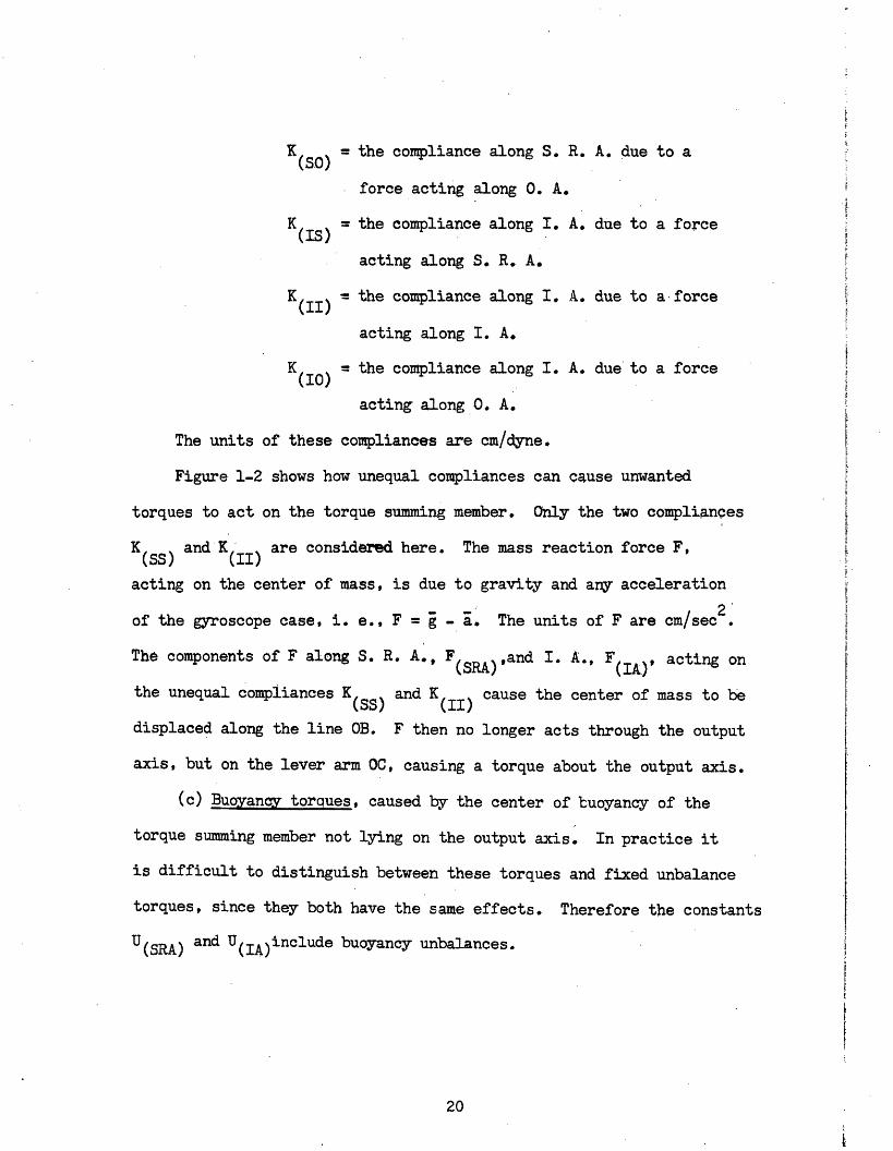
K(SO) = the compliance along S. R. A. due to a(SO)
force acting along 0. A.
K() = the compliance along I. A. due to a force
acting along S. R. A.
K(II) - the compliance along I. A. due to a force
acting along I. A.
K(I0) = the compliance along I. A. due to a force(I0)
acting along 0. A.
The units of these compliances are cm/dyne.
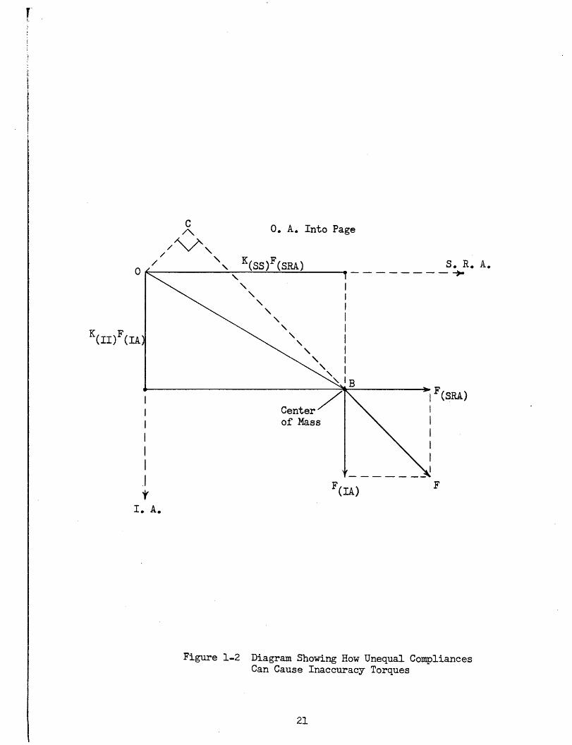
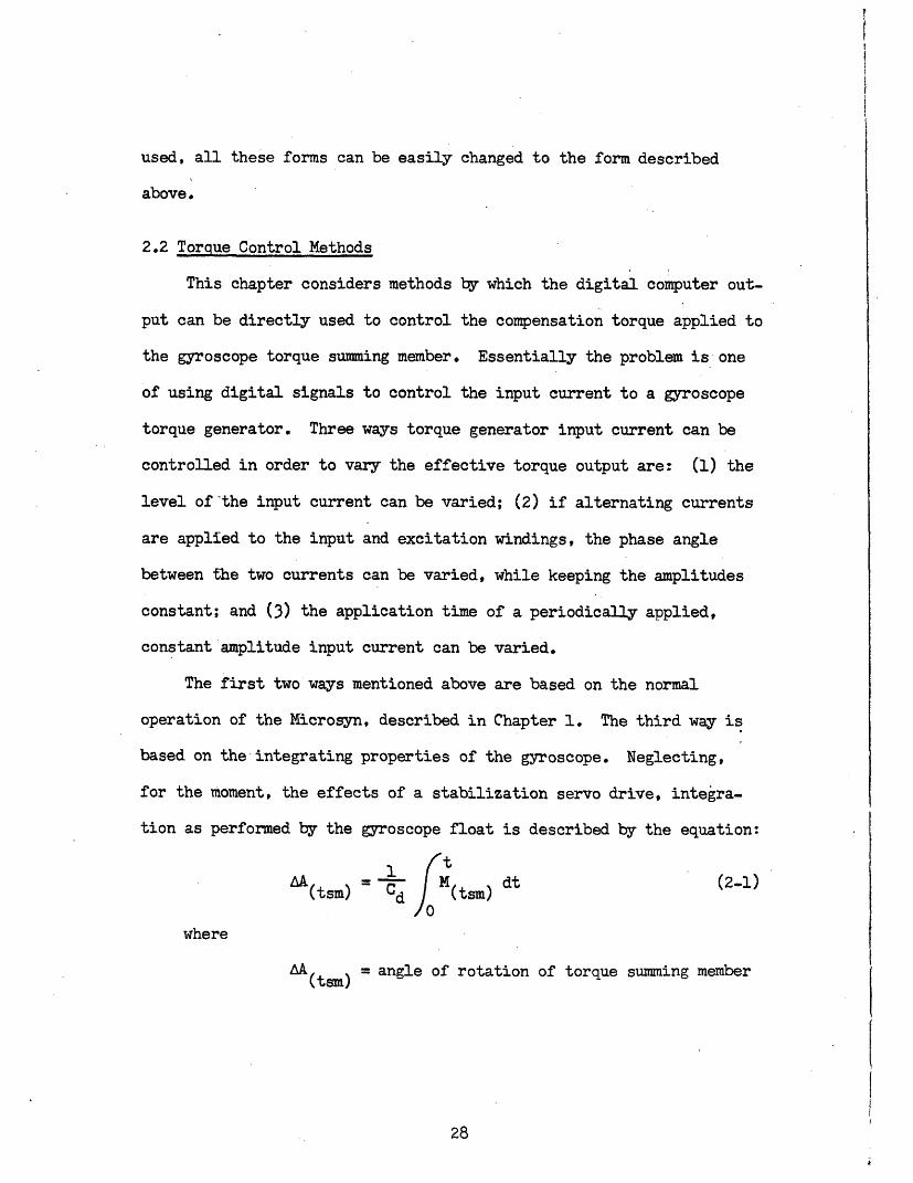
Figure 1-2 shows how unequal compliances can cause unwanted
torques to act on the torque summing member. Only the two compliances
K(SS) andK(I) are considered here. The mass reaction force F,
acting on the center of mass, is due to gravity and any acceleration
2'of the gyroscope case, i. e., F = g - a. The units of F are cm/sec
The components of F along S. R. A., F(SRA),and I A F(IA) acting on
the unequal compliances K(SS) and K(II) cause the center of mass to be
displaced along the line OB. F then no longer acts through the output
axis, but on the lever arm OC, causing a torque about the output axis.
(c) Buoyancy torques, caused by the center of buoyancy of the
torque summing member not lying on the output axis. In practice it
is difficult to distinguish between these torques and fixed unbalance
torques, since they both have the same effects. Therefore the constants
U(SRA) and U (IA)include buoyancy unbalances.
20
I
C
/A\1\0. A. Into Page
0
K(II)F(IA
Center of Mass
.1
I. A.
Figure 1-2 Diagram Showing How Unequal CompliancesCan Cause Inaccuracy Torques
21
S. R. A.- _ -t
II
I
I
I
I
II
I
F(IA)F
F(SRA)
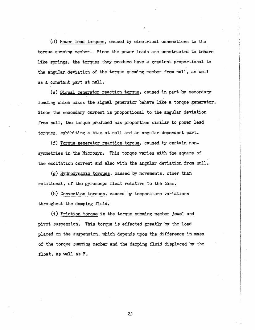
(d) Power lead torques, caused by electrical connections to the
torque summing member. Since the power leads are constructed to behave
like springs, the torques they produce have a gradient proportional to
the angular deviation of the torque summing member from null, as well
as a constant part at null.
(e) Signal generator reaction torque, caused in part by secondary
loading which makes the signal generator behave like a torque generator.
Since the secondary current is proportional to the angular deviation
from null, the torque produced has properties similar to power lead
torques, exhibiting a bias at null and an angular dependent part.
(f) Torque generator reaction torque, caused by certain non-
symmetries in the Microsyn. This torque varies with the square of
the excitation current and also with the angular deviation from null.
(g) ydrodynamic torques, caused by movements, other than
rotational, of the gyroscope float relative to the case.
(h) Convection torques, caused by temperature variations
throughout the damping fluid.
(i) Friction torque in the torque summing member jewel and
pivot suspension. This torque is effected greatly by the load
placed on the suspension, which depends upon the difference in mass
of the torque summing member and the damping fluid displaced by the
float, as well as F.
22
i.
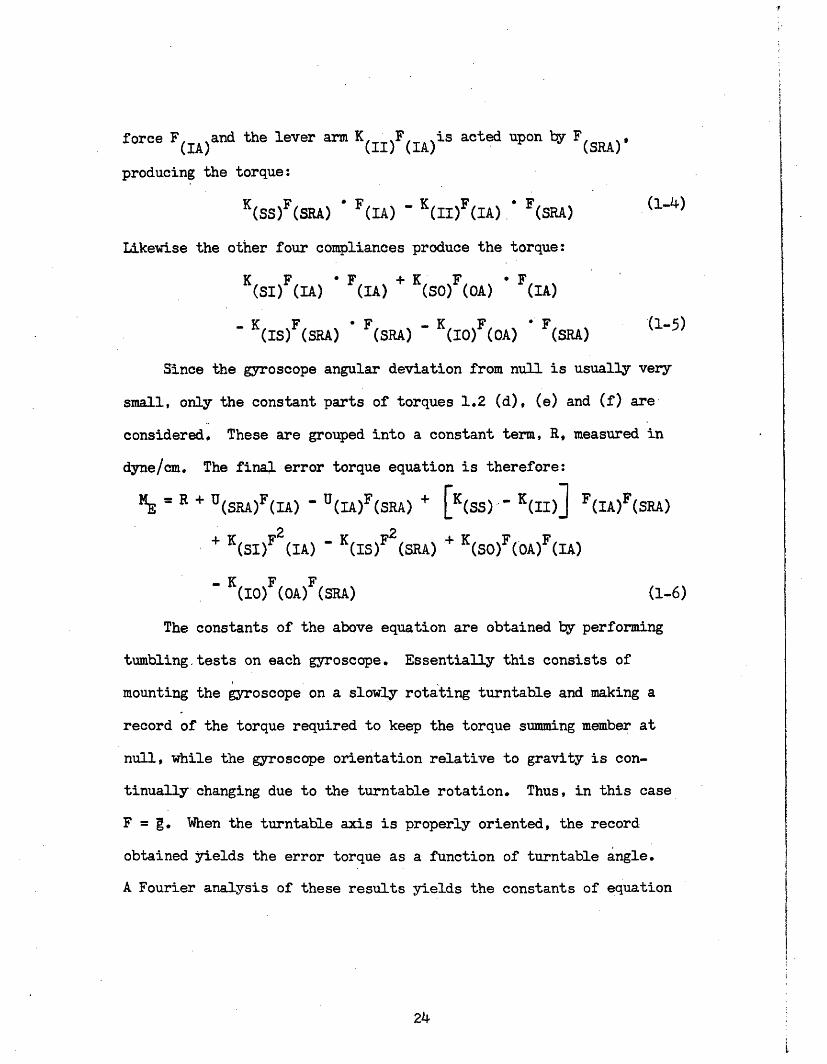
1.3 Error Torque Equation
Uncertainty torques are unpredictable not only as to their
magnitudes, but in many instances also their origins. Thus, in
several cases the above mentioned torques contribute to both the
error and uncertainty torques. Torques 1.2 (g), (h) and (i) are,
for the most part, uncertainty torques. Therefore the error torques
are usually considered to be composed of those described in 1.2 (a)
through (f). The equation describing these torques is now derived.
Torques 1.2 (a), (b) and (c) are dependent upon the specific
force acting on the gyroscope. The force F is resolved into com-
ponents lying along S. R. A., I. A. and 0. A. These force com-
ponents are considered positive when they are directed along these..axes
in the positive directions as determined by the arrows of Figure 1-1.
Unbalances and compliance deflections are considered positive if they
lie along the positive axes.
Referring to Figure 1-1, the two unbalances considered give rise
to the torque about 0. A.:
U(SRA)F(IA) - (IA)F(SRA) (1-3)
The torque about O. A. due to unequal compliances is obtained
by referring to Figure 1-2. The deflections due to only two of the
compliances considered in 1.2 (b) are shown in the diagram, but the
same reasoning is easily extended to include the other four. The
lever arm produced by the deflection K( SSF(sRA) is acted upon by the(Ss) (s )
23
IcIII
I
I
force FA)and the lever arm K )F( is acted upon by F(IA)' (II) (IA) (SRA)"
producing the torque:
K(ss)F(IA) (I')(IA) F(RA) (SRA )
Likewise the other four compliances produce the torque:
K(sI)F(IA) F(IA) + K(s(IA) ' F(IA)
_ K(sF(SRA) F(SRA) K(IO)F(OA) (SRA)
Since the gyroscope angular deviation from null is usually very
small, only the constant parts of torques 1.2 (d), (e) and (f) are
considered. These are grouped into a constant term, R, measured in
dyne/cm. The final error torque equation is therefore:
R + (SRA) F(IA) U(IA)F(RA) + [K(s) K(II) F(IA)F (SRA)
+K(sI)- (A K(Is)F (sRA) + K(so)F (A) (IA)
(I0) (OA) (RA) (1-6)
The constants of the above equation are obtained by performing
tumbling.tests on each gyroscope. Essentially this consists of
mounting the gyroscope on a slowly rotating turntable and making a
record of the torque required to keep the torque summing member at
null, while the gyroscope orientation relative to gravity is con-
tinually changing due to the turntable rotation. Thus, in this case
F = g. When the turntable axis is properly oriented, the record
obtained yields the error torque as a function of turntable angle.
A Fourier analysis of these results yields the constants of equation
24
L
i
I
(16). These tests are covered in great detail in references 1 and 2.
1.4 Analog Drift Compensation
In an analog drift compensation system, the various force com-
ponents are obtained from linear accelerometers aligned along the
three gyroscope input axes, which also correspond to the three major
axes of each gyroscope. These force components are represented by
various voltage levels. The associated analog computers, one for each
gyroscope, are composed of amplifiers, potentiometers and related com-
ponents. The error constants are put into the computers by setting
appropriate potentiometers.. Each computer output is a voltage, which
is fed to a matching amplifier. The output of the matching amplifier
goes to the torque generator input winding of the associated gyroscope.
In many cases, to simplify equipment, not all of the terms of
equation (1-6) are calculated. Some of the compliance terms are
found to contribute only a small amount to gyroscope drift and these
may be eliminated.
25
I

cR6
Chapter II
DIGITAL DRIFT COMPENSATION METHODS
2.1 System Computer
In a digital drift compensation system the compensation torque
required for each gyroscope is calculated by a digital computer.
Many possibilities exist as to the type of digital computer to be
used and the form that the computer output takes. The intention of
this thesis is not to determine the type of computer to be used. This
is determined by the requirements of the rest of the inertial system.
Therefore a general type of digital computer is assumed to be used
that operates in the following manner. Periodically sampled digital
specific force data from the inertial system accelerometers are fed
into the computer. By using this data and the required gyroscope
error constants stored in its memory, the computer calculates the
compensation torque magnitude from equation (1-6). The compensation
torque direction is opposite that of (1-6). This is read out in
parallel form as a binary number whose magnitude is equal to the
torque magnitude and one digit of which represents the torque direction.
.The number of digits in the binary number depends upon the accuracy
desired. The rate at which new torque calculations are made depends
upon how closely changes in the error torque need to be followed.
While the output can take other forms, depending on the type computer
27
used, all these forms can be easily changed to the form described
above.
2.2 Torque Control Methods
This chapter considers methods by which the digital computer out-
put can be directly used to control the compensation torque applied to
the gyroscope torque summing member. Essentially the problem is one
of using digital signals to control the input current to a gyroscope
torque generator. Three ways torque generator input current can be
controlled in order to vary the effective torque output are: (1) the
level of the input current can be varied; (2) if alternating currents
are applied to the input and excitation windings, the phase angle
between the two currents can be varied, while keeping the amplitudes
constant; and (3) the application time of a periodically applied,
constant amplitude input current can be varied.
The first two ways mentioned above are based on the normal
operation of the Microsyn, described in Chapter 1. The third way is
based on the integrating properties of the gyroscope. Neglecting,
for the moment, the effects of a stabilization servo drive, integra-
tion as performed by the gyroscope float is described by the equation:
t1
A(tsm) t) dt (2-1)
where
AA(tsm ) = angle of rotation of torque summing member
28
Cd = damping coefficient of gyroscope float
M(tsm) - forcing torque acting on the torque summing
member
Only two torques acting on the torque summing member are con-
sidered here, the error torque and compensation torque. Thus, the
precessional torque and any command torques applied through the
torque generator are omitted, since their presence does not effect
the problem. Also uncertainty torques are omitted, since their
presence cannot be predicted. Equation (2-1) then becomes:
(A ddt + dt (2-2)(tsm) Cddt+
where
MC = compensation torque
Therefore, in order that there be no net angular deviation of the
torque summing member due to error torques occurring during the
time interval O-.t, it is sufficient that:
t /t
dt dt (2-3)E C
In this case A(t ) will not necessarily be zero during the whole timeIn this case A will not necessarily be zero during the whole time
interval, since this would require: M(t) = - M(t). Also Atsm
willnot necessarily be zero at time t, since the final position of
the torque summing member is approached assymptotically at a rate
depending on the time constant of the gyroscope.
29
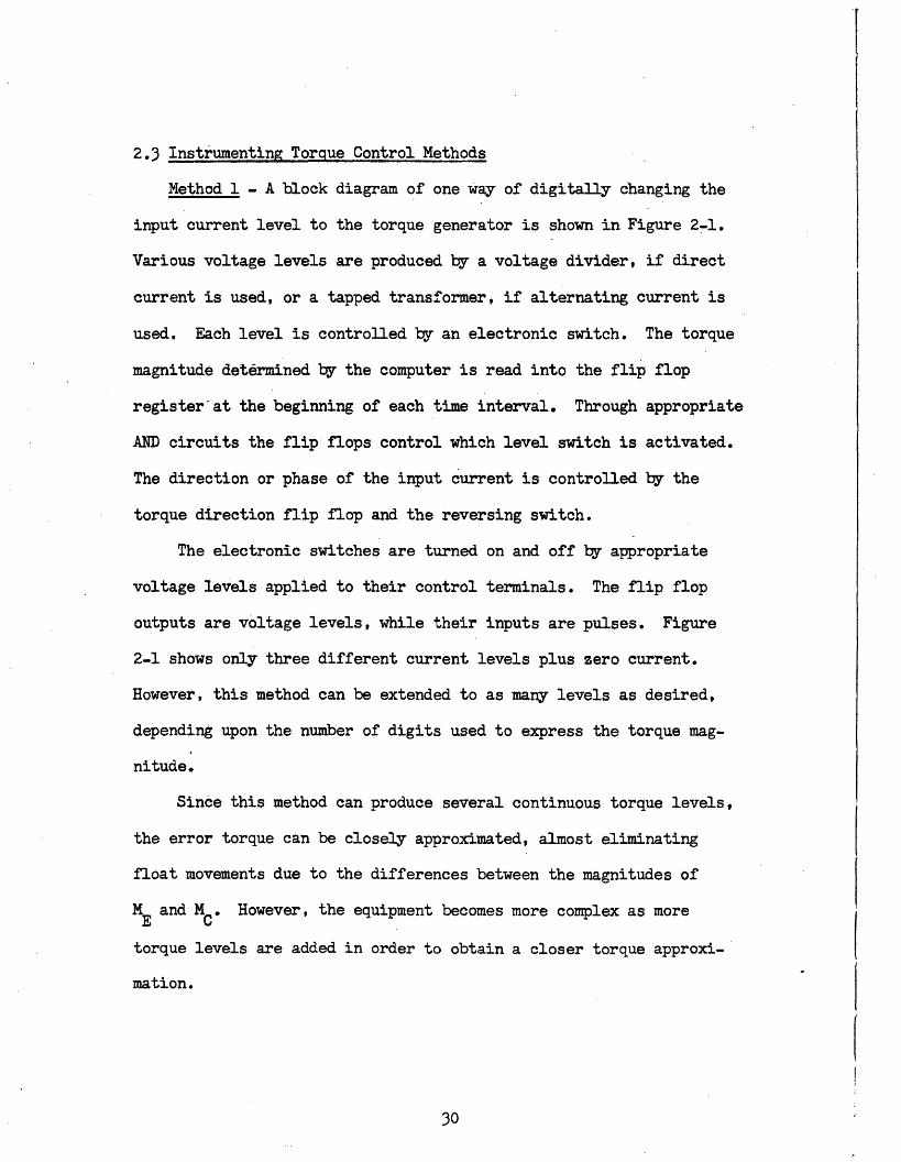
2.3 Instrumenting Torque Control Methods
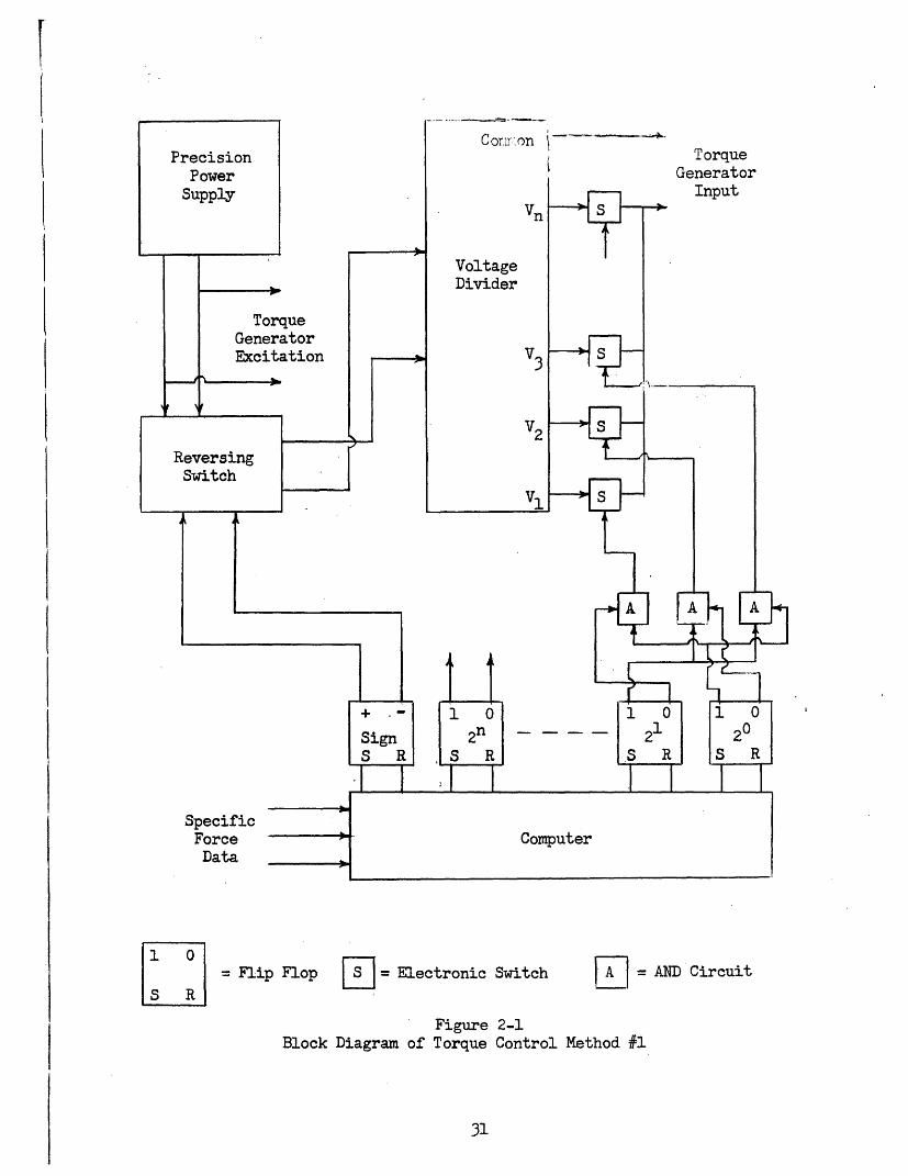
Method 1 - A block diagram of one way of digitally changing the
input current level to the torque generator is shown in Figure 2-1.
Various voltage levels are produced by a voltage divider, if direct
current is used, or a tapped transformer, if alternating current is
used. Each level is controlled by an electronic switch. The torque
magnitude determined by the computer is read into the flip flop
register at the beginning of each time interval. Through appropriate
AND circuits the flip flops control which level switch is activated.
The direction or phase of the input current is controlled by the
torque direction flip flop and the reversing switch.
The electronic switches are turned on and off by appropriate
voltage levels applied to their control terminals. The flip flop
outputs are voltage levels, while their inputs are pulses. Figure
2-1 shows only three different current levels plus zero current.
However, this method can be extended to as many levels as desired,
depending upon the number of digits used to express the torque mag-
nitude.
Since this method can produce several continuous torque levels,
the error torque can be closely approximated, almost eliminating
float movements due to the differences between the magnitudes of
ME and MC . However, the equipment becomes more complex as more
torque levels are added in order to obtain a closer torque approxi-
mation.
30
Cor]rq.o.n l ' 'A
= Flip Flop - = Electronic Switch
[S J
A - AND Circuit
Figure 2-1Block Diagram of Torque Control Method #1
31
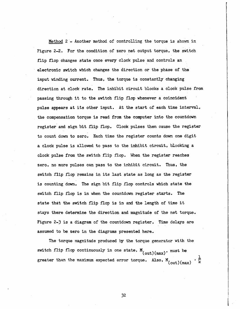
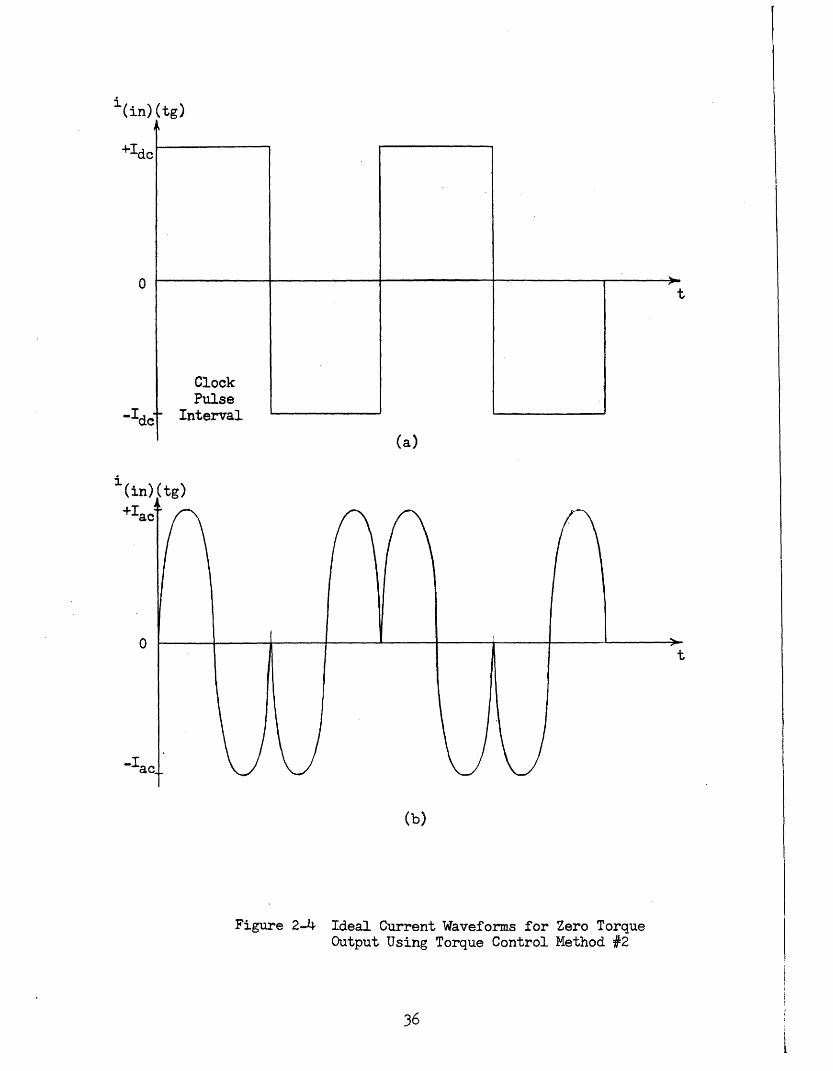
Method 2 - Another method of controlling the torque is shown in
Figure 2-2. For the condition of zero net output torque, the switch
flip flop changes state once every clock pulse and controls an
electronic switch which changes the direction or the phase of the
input winding current. Thus, the torque is constantly changing
direction at clock rate. The inhibit circuit blocks a clock pulse from
passing through it to the switch flip flop whenever a coincident
pulse appears at its other input. At the start of each time interval,
the compensation torque is read from the computer into the countdown
register and sign bit flip flop. Clock pulses then cause the register
to count down to zero. Each time the register counts down one digit
a clock pulse is allowed to pass to the inhibit circuit, blocking a
clock pulse from the switch flip flop. When the register reaches
zero, no more pulses can pass to the inhibit circuit. Thus, the
switch flip flop remains in its last state as long as the register
is counting down. The sign bit flip flop controls which state the
switch flip flop is in when the countdown register starts. The
state that the switch flip flop is in and the length of time it
stays there determine the direction and magnitude of the net torque.
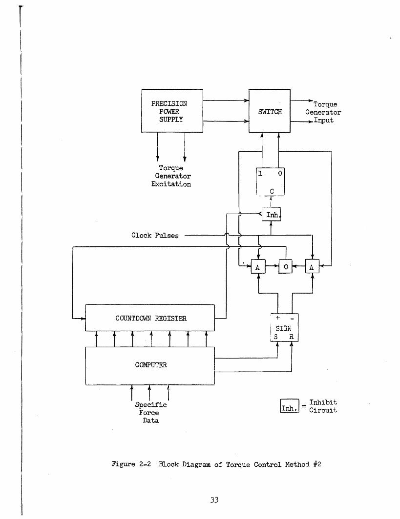
Figure 2-3 is a diagram of the countdown register. Time delays are
assumed to be zero in the diagrams presented here.
The torque magnitude produced by the torque generator with the
switch flip flop continuously in one state, M( t) , must be
greater than the maximum expected error torque. Also, Mtax) k
32
Specific = CirForce
Data
Figure 2-2 Block Diagram of Torque Control Method #2
O1ll
cuit
33
F
I
Inputs From Computer
Figure 2-3 Block Diagram of Countdown Register
34
,V~
must equal one digit in the least significant column of the computed
compensation torque, where k is the number of clock pulses per com-
putation interval.
Either direct or alternating current can be used on the two
torque generator windings. If alternating current is used, the
clock pulses must be synchronized at some multiple of the current
frequency. Also they must occur when the torque generator input
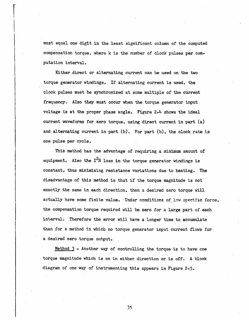
voltage is at the proper phase angle. Figure 2-4 shows the ideal
current waveforms for zero torque, using direct current in part (a)
and alternating current in part (b). For part (b), the clock rate is
one pulse per cycle.
This method has the advantage of requiring a minimum amount of
equipment. Also the I2R loss in the torque generator windings is
constant, thus minimizing resistance variations due to heating. The
disadvantage of this method is that if the torque magnitude is not
exactly the same in each direction, then a desired zero torque will
actually have some finite value. Under conditions of low secific force,
the compensation torque required will be zero for a large part of each
interval. Therefore the error will have a longer time to accumulate
than for a method in which no torque generator input current flows for
a desired zero torque output.
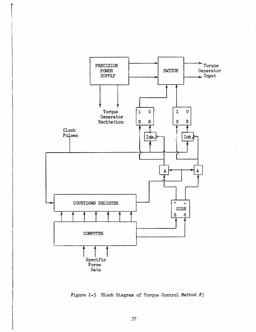
Method 3 - Another way of controlling the torque is to have one
torque magnitude which is on in either direction or is off. A block
diagram of one way of instrumenting this appears in Figure 2-5.
35
ClockPulse
Interva
(b)
Figure 2-4 Ideal Current Waveforms for Zero TorqueOutput Using Torque Control Method 2
36
0
0
b
k CL
I
V
SpecificForceData
Figure 2-5 Block Diagram of Torque Control Method #3
37
As in the previously desribed method, the computer reads the torque
into the countdown register and sign bit flip flop at the start of
each time interval. Normally the two switch flip flops are kept in
the zero position by clock pulses appearing at the reset inputs. When
the register starts counting down, clock pulses are allowed to appear
at the set input of one of the flip flops, while blocking the pulses
from the reset input through the inhibit circuit. The sign bit flip
flop determines which of the two switch flip flops the pulses set.
After the countdown register reaches zero, the clock pulses again
appear at the reset inputs of both flip flops. Thus, for a torque
other than zero, the switch is on in one direction for a certain
amount of time at the start of each interval and then off for the
rest of the interval.
This method has the advantages of being simple to instrument
and of producing exactly zero torque when this condition is desired.
As in method 2, the input current level to the electronic switch is
1such that M(out)(max) ' = least significant digit of computed
torque.
Method 4 - The previous two methods for controlling the torque
depend completely upon the integration action of the gyroscope float
for the time integration of the individual error torque computations.
That is, as soon as the required compensation torque is calculated by
the computer, it is applied to the gyroscope. Another method is to
integrate the torque digitally over a period of time until a point
38
is reached when the compensation torque required is equal to the
single torque magnitude available. Then applying this torque magni-
tude for one time interval cancels out the total effects the error
torque has caused over several intervals.
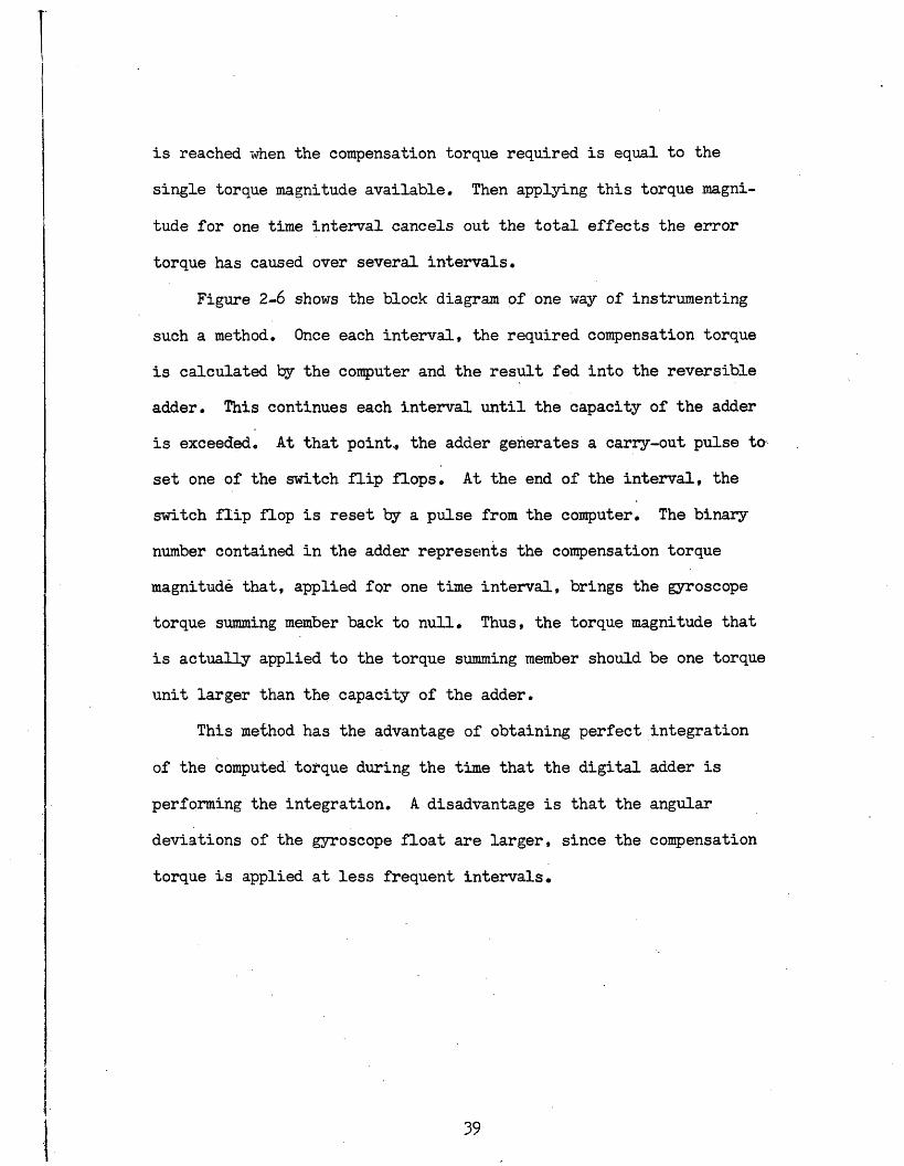
Figure 2-6 shows the block diagram of one way of instrumenting
such a method. Once each interval, the required compensation torque
is calculated by the computer and the result fed into the reversible
adder. This continues each interval until the capacity of the adder
is exceeded. At that point, the adder generates a carry-out pulse to
set one of the switch flip flops. At the end of the interval, the
switch flip flop is reset by a pulse from the computer. The binary
number contained in the adder represents the compensation torque
magnitude that, applied for one time interval, brings the gyroscope
torque summing member back to null. Thus, the torque magnitude that
is actually applied to the torque summing member should be one torque
unit larger than the capacity of the adder.
This method has the advantage of obtaining perfect integration
of the computed torque during the time that the digital adder is
performing the integration. A disadvantage is that the angular
deviations of the gyroscope float are larger, since the compensation
torque is applied at less frequent intervals.
39
SpecificForce
no4.
Figure 2-6 Block Diagram of Torque Control Method #4
40
l
Chapter III
DEVIATIONS OF DIGITAL COMPENSATION
FROM THE IDEAL
3.1 Introduction
In Chapter II, digital compensation was shown to depend upon in-
tegration by the gyroscope torque summing member. At that time the
effects of any stabilization servo drive associated with the gyroscope
when it is used in an inertial system were neglected. A stabilization
servo, along with the gyroscope, acts as an integrating drive or space
integrator. The integration processes of the gyroscope torque summing
member and stabilization servo differ considerably. Their individual
contributions to the integration of torques on the torque summing
member also differ greatly.
The equation describing integration by the torque summing member,
repeated here for convenience, is:
tAA~t m = (2-1)
(tm C (tsm) C _dt
In operation JA(tsm) is limited to a very small value by action of
the stabilization servo drive. One function of this drive is to act
as an elastic restraint on the gyroscope torque summing member to
keep it operating at null. How well this function is performed
41
I
determines how large IA(t) may become and therefore how much
integration is performed by the viscous shear process in the gyroscope.
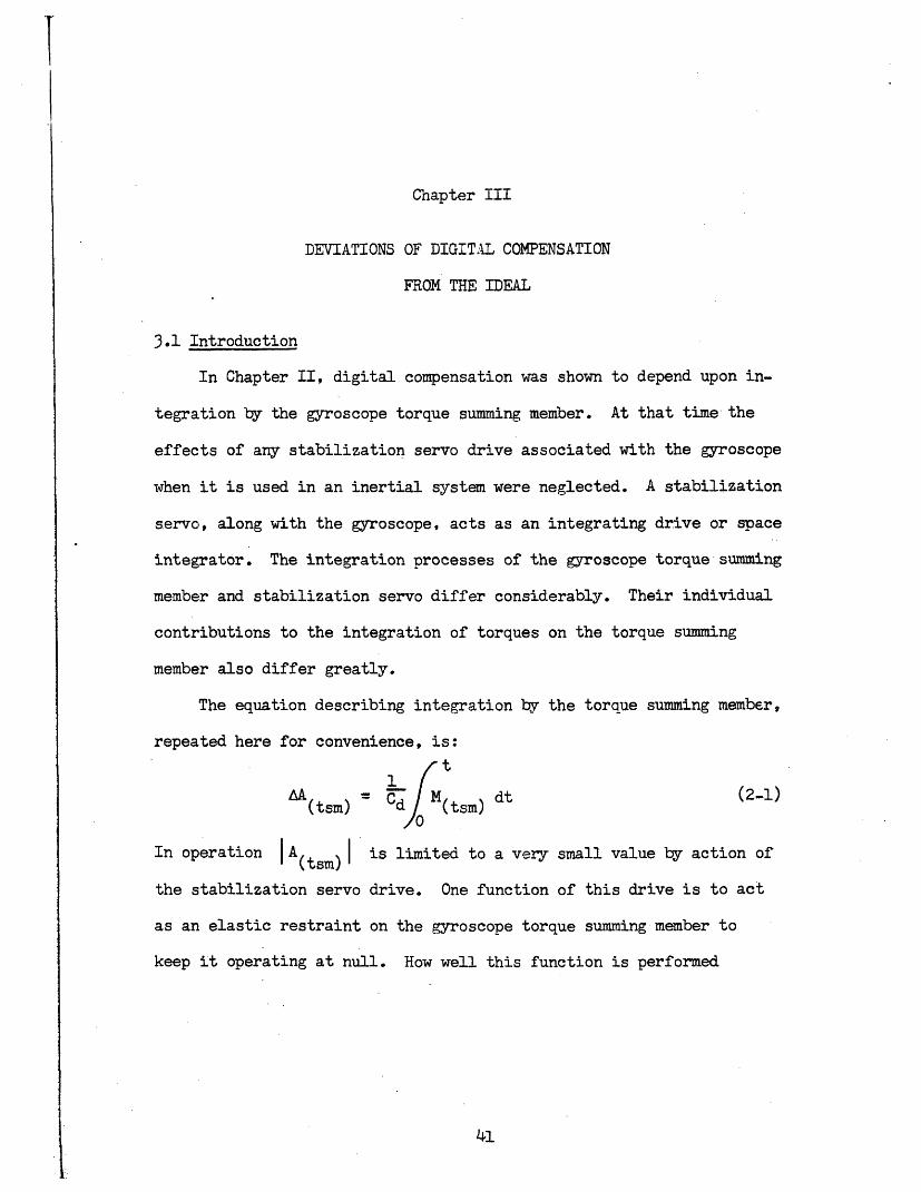
A block diagram of the essential components of a single-axis
stabilization servo drive appears in Figure 3-1. In an inertial
navigation system three of these drives are generally required. While
the actual servo instrumentation of a three-axis gimbal system is more
complex than merely having three independent single-axis drives, the
operation of each individual drive can be looked upon as being similar
to Figure 3-1. Besides providing elastic restraint for the gyroscope
torque summing member, the stabilization servo drive also produces,
under steady-state conditions, an angular velocity about the gyroscope
input axis proportional to the torque produced by the torque generator.
For an ideal servo drive, this velocity is:
W ! Ltaj_ (3-1)CI(cm) = H
where
I(cm) = angular velocity of controlled member
(gyroscope and platform on which it is
mounted) about gyroscope input axis, relative
to inertial space
H = angular momentum of gyro wheel
Hence:t
AA (tg) dt (3-2)
0/
42
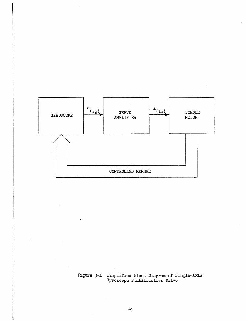
e(sg) (tm)
CONTROLLED MEMBER
Figure 3-1 Simplified Block Diagram of Single-AxisGyroscope Stabilization Drive
43
1
GYROSCOPESERVO
AMPLIFIER
/
TORQUEMOTOR
- -
.A
where
AA - rotation of controlled memberI(cm)
For an ideal servo drive with infinite loop gain, no gimbal bearing
friction and zero null indication by the gyroscope signal generator,
A(tsm) is always zero. All of the torque integration is therefore
performed by the servo drive. However, for an actual servo drive in
which all of the above quantities are finite, the servo drive requires
that IA(tsm)l have a certain minimum value, IA(tsm)(min) before it
can respond. This minimum angular deviation corresponds to the gyro-
scope signal generator output level that produces a servo drive torque
that just overcomes the gimbal bearing friction. In actual servo
drives, this deviation may be several seconds of arc. During the time
that IA(tsm)l is less than IA(tsm)(min) , all torque integration is
done by the gyroscope torque summing member.
The controlled member position is generally used as an angular
reference in inertial systems. Therefore movements of the gyroscope
torque summing member do not effect the angular reference until they
are transmitted, via the stabilization servo, to the controlled member.
Hence if the digital compensation torque is applied in such a manner
that A(tsm)I is always less than IA(tsm)(min) , ignoring pre-
cessional torques, angular deviations of the torque summing member
from null, due to the differences between the error torque and com-
pensation torque, will not effect the angular reference. If this type
44
l
of operation is assumed, then the effects of the stabilization servo
drive on the operation of the digital compensation system can be
ignored. The only times that the servo drive will perform angular
integrations is when precessional torques or command torques cause
the torque summing member to rotate or when rotations caused by com-
pensation torque inaccuracies or uncertainty torques build up to the
point that JA(tsm)(min)l is exceeded. In view of this, only torque
integration performed by the gyroscope torque summing member will be
considered here as to its possible effects on digital compensation.
Non-linearities and imperfections in components can cause
deviations in digital compensation performance from the ideal. The
more important of these causes are analyzed in this chapter. In some
of the analyses, in order to consider certain effects, the torque
acting on the torque summing member due to the combination of error
and compensation torques must be known. This torque, of course, de-
pends upon many factors and is always changing. Therefore to facilitate
the analyses a certain torque pattern occurring during a given time
interval is considered as typical. This torque pattern is given here
and then referred to as needed.
In general, the compensation torque is constant in amplitude over
a given time interval whereas the drift torque is not. Also, the com-
pensation torque magnitude is generally greater than that of the error
torque. Figure 3-2 shows a constant compensation torque of magnitude
M occurring during the time interval to--*t, and an error torque of
45
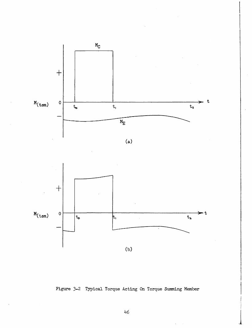
+
0
-
0
to- t.
t,
(a)
to
Figure 3-2
t2t,
(b)
Typical Torque Acting On Torque Summing Member
46
M(tsm)
M(tsm)
I1
l
u-
magnitude ME, not necessarily constant, occurring continuously. The
combined torques produce the net torque acting on the torque summing
member shown in part (b). This is the typical torque. The torque has
the following properties:
IM > I M I (maximum) and MC (t, - t) =- dt (3-3)
If this torque were applied to a perfect gyroscope, AA(tsm)(tof ta)
would equal zero, where A(tsm)(to_ _t) is the angular change of the
torque summing member over the interval Lt-- to. Likewise:
AA(tsm)(t-- t, ) -AA(tsm) (tt ) (--)
3.2 Effects of Non-Newtonian Damping Fluid
The damping fluid used in gyroscopes is assumed to exhibit perfect
Newtonian qualities. That is, its viscosity is independent of all in-
fluences except temperature. It is further assumed that the fluid flow,
due to any float movements, is completely laminar. Under these condi-
tions, with constant fluid temperature, the viscous resisting torque
exerted on the gyroscope float, as it rotates relative to the case, is
given by the equation:
Md =- Cdtm) (3-5)dt
where
Md = viscous torque exerted on the
float by the damping fluid.
47
Rewritten, this equation becomes:
AtA m dt (3-6)
This relationship is the source of the integrating properties of the
gyroscope.
If either or both of the above assumptions concerning the damping
fluid is not realized in practice, the integration performed by the
gyroscope is affected. In an inertial system not employing digital
drift compensation, anomalies in gyroscope integration do not greatly
effect system performance, since, as pointed out previously, practically
all angular integration is performed by the stabilization servo drives.
However, when digital drift compensation is employed, integration per-
formed by the gyroscope float should prove more critical, since such
compensation depends heavily on these integrating properties. The
number of float movements is greatly increased when digital compensation
is used.
In order to determine the effects of a non-Newtonian damping fluid
or non-laminar flow on digital drift compensation, a damping torque is
considered that is not directly proportional to the relative angular
velocity of the float and case. Such a condition would exist for non-
laminar flow or for a fluid whose viscosity is a function of shear rate.
An arbitrary non-linearity will be assumed such that:
:d = C (tsm) (3-7)L dt
where
b 1
For a constant forcing torque, M(tsm), under steady-state conditions,
M(tsm) = - Md. Due to the high damping in gyroscopes the torque sum-
ming member time constant is very small and hence steady-state conditions
are reached quite fast. Therefore transient effects will be ignored
here.
For the typical torque of Figure 3-2:
M + ME Cd dsm)] b(3-8)
Solving for A(tsm) yields:
b +
If ME is constant during the interval (t_ t-) :
dt (3-9)
b 1 1
A(tsm)(to(--t) = []b [ + ME I. (t - t) -ME (t- t(3-10)
For the typical torque of Figure 3-2, with ME constant:E
to - to
ta - t,
Therefore,
AA(tsm)(t, t )
(3-11)1Ml
MC + ME1
IMc(t 2- t) [F 1- _- b
(Cd - (3-12)
49
Thus, AA(tsm)(to-_t2) - O only for the isolated case when
INCI 2 ME .· For all other cases A(tsm)(t has some value
which represents the error introduced by imperfect float integration
during the interval t---t 2 . This error accumulates as long as the
error torque remains in the same direction.
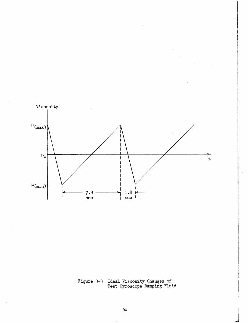
3.3 Effects of Damping Fluid Temperature Changes
The gyroscope damping fluid temperature is usually maintained with-
in certain limits by a system of electric heating coils located around
the fluid chamber. Temperature sensing devices control the amount of
current flowing to these heating coils. In the gyroscope used for this
thesis, a temperature sensitive microswitch, which was either off or on,
controlled the current to the heaters.
One formula for the viscosity of a fluid as a function of tempera-
ture is given by:
Alog = + B (3-13)
where
T = absolute temperature of fluid
A, B = fluid constants
Other formulas exist, all of which relate viscosity exponentially with
temperature. Within a narrow temperature range, however, a good approxi-
mation is obtained by using a linear relationship between viscosity and
temperature.
For the gyroscope used for this thesis, the viscosity of the
50
l
damping fluid increases approximately 4% for each drop of 1° F in
temperature in the immediate vicinity of the operating temperature,
This change can therefore be approximately described by the formula:
b= P (1 + 0.04 [To - T ) (3-14)
where
- viscosity at specified operating temperature, To
- viscosity at actual operating temperature, T
The design specifications of this gyroscope called for temperature
control limits of 0.2° F. The fluid temperature therefore fluctuated
between T + 0.20 and T - 0.2° . Under the ambient conditions of normal
room temperature, the duty cycle of the microswitch was measured to be
approximately 1.8 seconds on and 7.8 seconds off.
If a linear rise and fall in fluid temperature between the opera-
ting temperature limits is assumed, then the damping fluid viscosity of
the gyroscope under consideration changes with time as shown in Figure
3-3. The maximum change in viscosity over each temperature cycle is
1.6%.
For a given forcing torque acting on the torque summing member,
1 1dA(tsm) is proportional to C and also to 1, since Cd is proportionaldt d
to p. The float therefore rotates faster when p is lower. If the
majority of the compensation torque pulses occur when A is higher than
pb or when is lower than P, errors in A are introduced.(tsm are intro rs cance
These errors are a source of uncertainty. In general the errors cancel
51
ty
Figure 3-3 Ideal Viscosity Changes ofTest Gyroscope Damping Fluid
52
I ;
I,
I
out over periods of time and therefore do not accumulate However, if
i out over periods of time and therefore do not accumulate. owever if
the compensation torque application cycle is some multiple of the fluid
temperature cycle, these errors may accumulate. In the worst case,
when compensation torque applications occur once each temperature cycle,
at the time of maximum or minimum viscosity, the error introduced in
A each cycle is:(tsm)
(E) (tsm) - (tsm)(max) (max) (15)
where
AA(tsm)(max) = maximum torque summing member deviation
with constant fluid temperature.
The damping fluid temperature is not uniform. Due to the distri-
bution of the heaters, temperature gradients are present throughout the
fluid. Therefore viscosity gradients are also present. The presence
of convection currents and changes in F make the effects of the viscosity
gradients practically impossible to analyze. These gradients are there-
fore a source of uncertainty torque.
3.4 Effects of Friction in Torque Summing Member Suspension
The pivot and jewel suspension of the gyroscope torque summing
member can be the source of undesired non-viscous friction torques.
These torques are partially dependent upon the suspension loading,
which in turn depends upon the buoyancy of the damping fluid and upon F.
The buoyancy of the damping fluid varies with its density., which is a
function of temperature. Therefore the suspension friction is not constant,
53I1'
but varies with F and fluid temperature.
For purposes of this discussion, the suspension friction torque,
M( f), is assumed to have a magnitudeM( f)(max)as long as the magni-
tude of Mc + ME is equal to or greater than this amount and to be equal
in magnitude to M + M otherwise. The direction of M(sf), of-course,
is opposite to that of MC + .
For the typical torque of Figure 3-2:
AA(tsm)(to -- ta) Cd tMc(t, - to) + t dt
(3-16)
If MC and ME are both greater than M(sf)(max ) then:
AA(tsm)(to .ta) Cd [ M(t, - t) +(dt
IM(sf)(ma) | (t- to) + |M(sf)(max)l (ti- t ) (3-17)
By definition the sum of the first two terms of (3-17) equals zero.
Therefore:
AA(tsm)(tO- ts) Cd I (sf)(max) I [(t- t) - (t, - t)](3-18)
In general (tn - t) (t, - to). The usual case is for (t - t,) to
be several times larger than (t, - t).
54
If is smaller than M(sf)(max ) , then:
(tsm)(t0-- t) [E(t, - to) + , dt
(sf)(max) | ( S to) tfi \ ] (3-19)
or,
A(tsm)(to--- t) Cd [ ( - IM(sf)(max)I ) (t, - to)
+ dit (3-20)
When ME is smaller than M (sf)(max), M will always be much greater
than both these torques. Therefore the result in both cases is an
error in A(tsm) in the direction of MC . This error accumulates as
as long as ME remains in the same direction.
3.5 Effects of A(tsm) Not being Zero
It has been shown that the mutual inductance of the Microsyn
torque generator excitation and input windings is proportional to
A(tsm ) . Thus, for finite excitation and input source impedances and
A (tsm) 0, cross-coupling currents flow in the two windings. The
torque produced by the torque generator then becomes:
M(tg) S(tg) [(ex)(tg)(ideal) (in)(tg)(ideal)
+ i(ex)(tg)(ideal) gi(ex)(tg) + i(in)(tg)(ideal)it(in)(tg)
+Si(ex)(tg) 8i(in)(tg)] (3-21)
55
*superscripts refer to Bibliography
i(ex)(tg) = i(ex)(tg)(idea:) + Si(in) (tg)
i(in)(tg) i(in)(tg)(ideal)+ gi(ex)(tg)
gi(ex)(t
$i(in)(t
where
v (ex)(t
and V(in)(t
(ML) (ex) (i
Z(equiv)(ex)(tg)
and Z(equiv)(in)(tg)
i(ex)(tg)(ideal)
i(in)(tg)(ideal)
·g) (()ex)(tl )(in) (3-2:
Z(equiv)(ex)(tg)Z(equiv)(in)(tg)
= V(in)(tg) O (ML)(ex)(in)- (3-2:
(equiv)(in)(tg) (equiv)(ex)(tg)
.g)
g) = open circuit voltages of the respective
torque generator winding power sources
C-)= angular frequency of the voltages
n) = mutual inductance of the two windings
2)
3)'
= equivalent impedances of the respective
torque generator windings. Each is equal
to the source impedance plus the winding
impedance.
(ex)(tg)Z(equiv)(ex)(tg)
(in)(tg
Z (equiv)(in)(tg)
(3-24)
(3-25)
56
where
Since the cross-coupling currents are generally very small compared to
the applied currents, the last term of (3-21), which is the product of
these two currents, is ignored. The mutual inductance is directly pro-
portional to A(tsm) and ideally zero at A(tsm) O. It can therefore
be written, (ML)(ex)(in) KML)A(tsm ), where K is a proportionality(ex) (in) (ML) (ML)
constant. Rewritten, equation (3-21) becomes:
(tg) ~ (tg)[ (ex)(tg)(ideal) (in)(tg)(ideal)
2 .K(ML)A(tsm)(ex)(tg)(ideal) Z (equiv)(in)(tg)
+ i2(in) (tg) (ideal) (ML) (tsm) (3-26)
Z(equiv) (in) (tg)
The last two terms on the right of (3-26) are directly proportional
to A (t . They represent a torque that aids the ideal torque of the
first term when A(tsm) is on one side of null and opposes the ideal
torque when A is on the other side of null. Thus these two terms(tsm)
cause an elastic torque to be added to the ideal torque. For torque
generator windint impedances usually encountered, this torque is
stable. Such a torque is undesirable for the proper operation of the
gyroscope, since it is a non-integrating elastic restraint acting on
the torque summing member.
When precession torques cause the torque summing member to rotate
57
1.
from null, this elastic torque tends to force the torque summing member
back to null. This introduces an error equal to the angle through which
the torque summing member moves toward null due to action of the elastic
torque. The error is opposite in direction to the precession torque.
Therefore as long as the precession torques remain in the same direction
the individual errors will accumulate.
In order to reduce the effects of cross-coupling currents the
equivalent impedances should be as high as possible. This requires
using sources with high output impedances.
Due to increasing mutual inductance with increasing IA(tsm) an
elastic torque is also produced by the signal generator Microsyn when
a finite load is placed on the secondary winding. For a resistive or
inductive load the elastic torque is stable. However, for a capacitive
load the torque becomes unstable. An unstable torque causes any de-
viations of the torque summing member from null to increase with time.
Any unstable elastic torque produced by the signal generator is generally
smaller in magnitude than the stable elastic torques produced by the
torque generator and electrical leads. Therefore the net elastic torque
on the torque summing member is stable.
3.6 Effects of Switching Errors and Transients
Equations (2-1 ) and (1-2) combine to give the torque summing mem-
ber rotation due to torque generator currents as:
AAt) = S(tg) ) i (3-27)(tsm) - Ca d (ex)(tg) (in)(tg)dt (
58
Therefore A(tsm) depends upon the waveshape of the input current as
well as its application time. Until now the input current has been
assumed to be either sinusoidal or constant during the time it is ap-
plied. In practice, however, transients may alter the waveshape of the
input current and therefore cause AA(tsm) to be different than desired.
Also timing errors in the application of the input current can effect
AA(tsm)' Since the excitation current is applied continuously, transients
and timing errors are not factors in its contribution to the torque.
In the torque control methods described in Chapter II, the torque
generator input current is controlled by electronic switches. Since
the torque generator windings are highly inductive, if direct current
is used a transient build-up of current to the desired level occurs when
the switch is turned on. A transient also occurs when the switch is
turned off.
A square voltage pulse applied to the torque generator input
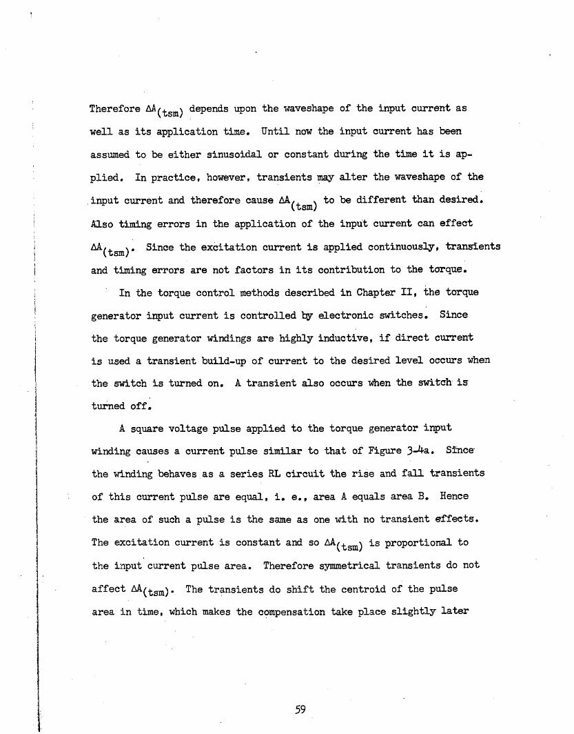
winding causes a current pulse similar to that of Figure 3-4a. Since
the winding behaves as a series RL circuit the rise and fall transients
of this current pulse are equal, i. e., area A equals area B. Hence
the area of such a pulse is the same as one with no transient effects.
The excitation current is constant and so AA(tsm) is proportional to
the input current pulse area. Therefore symmetrical transients do not
affect A(tsm). The transients do shift the centroid of the pulse
area in time, which makes the compensation take place slightly later
59
_v C ' t~~~~~~~~~~~~~~~~~~~~~~~~~~~~~~~~4
(a)(a)
P ^ t..1+h e _+ -._4|
Current
(b)
Figure 3-4 Torque Generator Input Current WaveformsShowing Transients Caused By Switching
60O
£
0
i
0
than planned. This effect, however, is not too significant.
Factors other than simple exponential build-up and decay affect the
current pulses, however. The transient characteristics of the electronic
switch and its associated flip flop also determine the pulse shape. The
circuits that were used for this thesis employed semiconductors. For
these circuits, the fall times of torque generator input current pulses
were greater than the rise times. This result was due in part to
minority carrier storage in the transistors. Such circuit non-Iinearities
cause the voltage pulse to be not perfectly square.
For actual switching circuits, then, the rise and fall transients
are generally not symmetrical. The area of such a pulse is not the same
as one without transients. Therefore the area is not directly propor-
tional to the nresumed annlication time of the voltage pulse. Since in__ -___ r- --
the torque control methods discussed, time is the controlled variable,
using equally spaced clock pulses, errors result if the voltage pulse
duration is different than that at which the torque is originally
calibrated.
Rqids r ranients, timing rrnrs affect the area of the current
pulses. If time delays occur between a turn-on command pulse and the
operation of the switch, the current pulse does not start until later
than desired. Similarly turn-off delays in the switch cause the current
pulse to end later than desired. For direct current pulses, the area
is not affected if both these delays are equal. If, however, they are
61
unequal, the area is either smaller or greater than desired, depending-
upon the size of each delay.
When alternating current is used on the torque generator windings
transients can be effectively eliminated by switching the input current
when the steady-state current sine wave pases through zero. This makes
the timing of the switch operation critical. Any deviation of the
switching times will cause transients. The equation of the current
resulting from the sudden application of a sinusoidal voltage to a
series RL circuit at t = 0 is:
E E -(R/L)ti = sin(wt + X- 8) - Zsin (- ) e
where
8 = steady-state phase angle between voltage and current
X = phase angle of voltage when voltage is applied
If the voltage is then removed at time t the current becomes:
E sin( + A - O)e (R/L)(t -to) E i(R/L)t
The transient terms are zero if = Figure 34b shows the approximate
The transient terms are zero if X= . Figure 3-4b shows the approximate
shape of such a current wave for two cycles of applied voltage, using
arbitrary X and 8. The resultant waveform consists of the sum of the
two transients and the steady-state term. Any errors in Ltsm) re-
sult only from the transient terms.
If the torque generator excitation current is in phase with the
steady-state input current, the error in AA(tsm) caused by transients
62
(E)A(tm) = S(tg)I(ex)(tg)I(n)t) in( t+ e)[sin(X-e)e dt(E)AI~sm) =2Cd Gl + sin(t+X-8) [sin( X-.)e- (RL)(t - t )]
(E)AA (). - R (tg)I(ex)(t)I(in)(tg) Ca
(2tmCd (R/L)2 + a
dt (3-30)
[sin (t, + X -e) - sin (X-8)] (3-31)
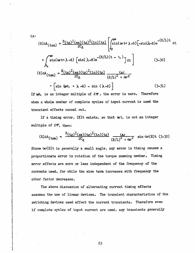
If at, is an integer multiple of 21r, the error is zero. Therefore
when a whole number of complete cycles of input current is used the
transient effects cancel out.
If a timing error, (E)t exists, so that t, is not an integer
multiple of 21r, then:
(E)AA(tsm) =S(tg)I(ex)(t)I(in) (tg)
2CdC( / z sin Wc(E)t (3-32)
(R/L)z +CO
Since CA(E)t is generally a small angle, any error in timing causes a
proportionate error in rotation of the torque summing member. Timing
error effects are more or less independent of the frequency of the
currents used, for while the sine term increases with frequency the
other factor decreases.
The above discussion of alternating current timing effects
assumes the use of linear devices. The transient characteristics of the
switching devices used affect the current transients. Therefore even
if complete cycles of input current are used, any transients generally
63
,2
do not cancel. However, any transients resulting from alternating cur-
rent switching errors usually are much smaller than transients resulting
from the use of direct current for the torque generator.
3.7 Quantization ErrorsMr13 a+; n1 +Ecj -Ttow 1rs -nlr* no Qnilh r ; -4ile><!a" -- ro4 -- --A -lrr1IY CLM L-LLIW LLir 1.L L J.L LJ.LU ,LL±.U 3JLLL - L...,Lk�LL. 3 A.% LJ.L%-V .LJ Y *
digital compensation still produces instaneous errors in float position.
These errors are caused by the net torque on the torque summing member
due to the compensation torque not being equal and opposite to the error
torque at all times. The net torque is caused by compensation torque
computation time lags and quantization errors due to the digital approxi-
mation of the error torque.
As mentioned previously, a digital compensation system should in-
sure that any instantaneous float position errors caused by quantization
should be less than JA(tsm)(min) . In this way the errors do not ap-
pear at the angular reference through operation of the stabilization
drive when no precession torque is present. If the compensation torque
is applied at equal intervals, then the maximum time between torque
applications is:
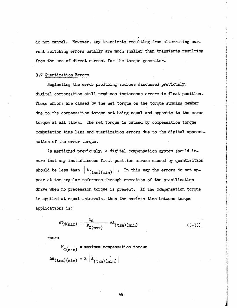
CdAtl(max) = C() tsm)(min) (3-33)
where
M(max) = maximum compensation torque
A(tsm)(min) = 21(tsm)(min)
I.1
If a precession torque acts on the torque summing member so that
IA(tsm)(min) is exceeded, the maximum instaneous error introduced to
the angular reference by compensation torque quantization is AA(tsm)(min).
Any value less than AtM(max) can be given to QAt with a proportionate
reduction in the maximum quantization error.
3.8 Computation Errors
Digital computations of the error torque must be made periodically
in order to determine the compensation torque required. The time be-
tween computations must be equal to or less than AtM. Besides this
restriction, other factors,which will be discussed, determine the com-
putation interval, Ate.
In making the computations, specific force measurements are re-
quired from the system accelerometers. In general digital accelerometers
produce output pulses proportional to velocity in either of the two
directions along their input axes. The equation for the velocity out-
put is:
v = Sv (n(+) - n(_)) = Svn (3-34)
where
v = velocity along positive direction of accelerometer
input axis
S = velocity increment per output pulse
n(+) and n(-) = number of output pulses for the positive and negative
input axis directions
Acceleration is obtained from this information by differentiating:
Sv na - (3-35)
Atc
The net number of output pulses, An, must be an integer. Therefore it
can be in error by as much as one pulse, Since the absolute error in
An is constant, the relative error can be reduced by increasing An.
AnThis can only be done by increasing At., since Ltc is determined by
the specific force.
Once an unbalance torque computation has been made, this computa-
tion is the only information the system has available concerning the
error torque until the next computation. Therefore if the error tor-
que changes during this interval, due to changes in specific force,
the available information is in error. This quantization error can be
reduced by reducing Atc.
Thus two conflicting requirements for Ate exist. The compromise
that is made in Atc between the above two requirements is dictated by
individual inertial system operating conditions. If it is known that
a system will encounter relatively long periods of constant specific
force with infrequent changes that last only for short intervals, Atc
should be large. However, a system that encounters frequent specific
force changes might require a smaller Atc. The effects of Atc on the
computed error torque are now analyzed.
In order to simplify the analysis of the effects of Atc on the
66
error torque computations, equation (1-6) is modified. Essentially
(1-6) contains three types of terms: a constant term, terms dependent
directly on specific force components and terms dependent on the products
of two specific force components. The equation can therefore be written,
for a force in any one direction, as:
K + F KF 2 (3-36)1 g 2 3 (3-36)
where
F = magnitude of mass reaction force on gyroscope
K2 and K3 = factors dependent upon direction of F
The equation, written with uncertainties in F, is:
ME K. 1(2 [F + (F)] + K3 [F + U(F)] (3-37)
Assuming that the uncertainty in F is due to the uncertainty in
An, i. e., any uncertainty in Atc is small compared to the uncertainty
in An, then:
F + U(F) - (An+l)Sv (3-38)Atc
When this substitution is made, (3-37) becomes:
An+ +ME K, + K2F + K3F2 + v (K2 + 2K3 ~tcc + K (3-39)
The relative uncertainty in ME is:
(1jc2 [2K3Sv(An+l) + K 3Sv2 ]+ (c ((340)
The relative uncertainty in ME increases as tc is decreased. This un-
67
certainty holds for each unbalance torque computation and the actual
error may be positive or negative. For constant F, generally one compu-
tation will be in error on the high side and the next computation in error
on the low side, since a velocity pulse which is omitted by one sampling
interval is gained by the next one. However, since ME is not a linear
function of F, equal positive and negative errors in two separate com-
putations of do not produce cancelling effects. Therefore when these
individual computations are summed up, either digitally or by the in-
tegrating action of the gyroscope, the compensation torque-time integral
will be larger than required.
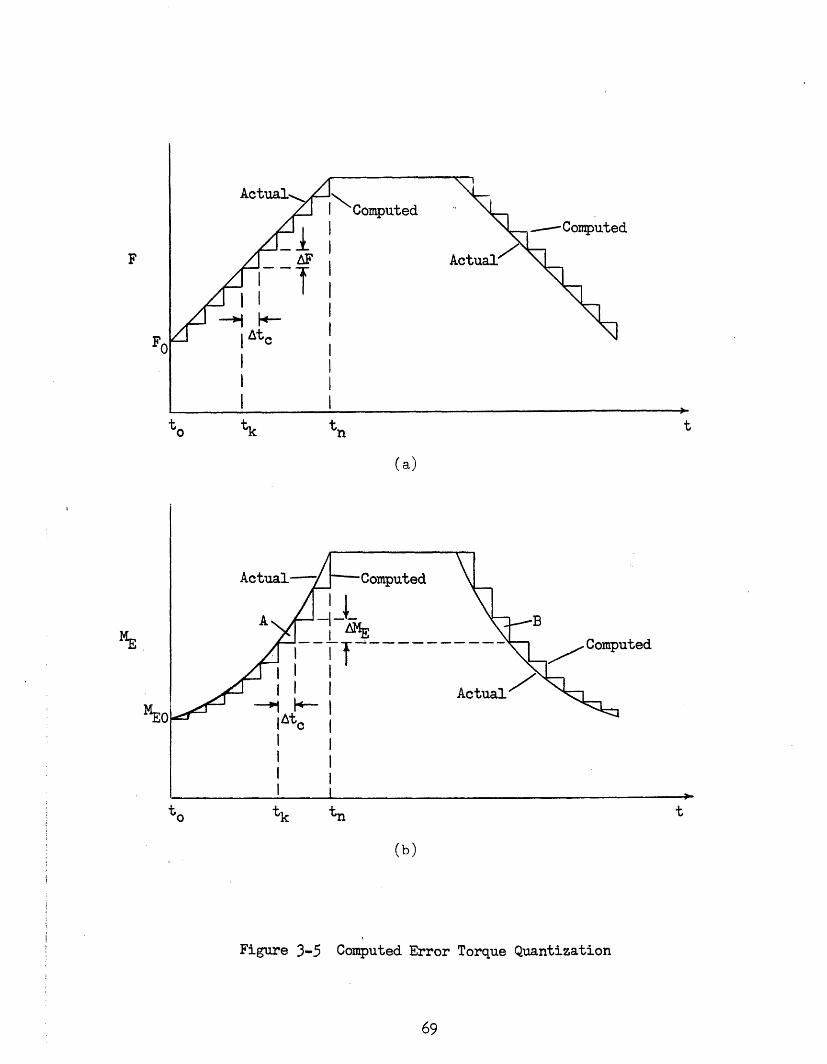
The effects of tc on the quantization error in F cannot be deter-
mined, since the actual variations of F with respect to time must be
known. However, the effects for an assumed linear variation of F with
respect to time can be found by considering Figure 3-5a. This figure
shows a linear increase andsdecrease in F, each of equal amounts and
dFoccurring over equal time intervals. Here d is constant and
dFF - Adtt, where F is the quantization error in F. The effect of
AF on ME computations can be found by substituting AF for U(F) in
(3-37). This gives:
(computed) = K + K2F + K3F2 F(K2 + 2K3F) + K3(AF)
2 (3-41)
Figure 3-56 shows the changes in M corresponding to the changes of
F in part (a). The effect of tc on the error torque quantization error,
AmE, can be seen from the following:
68
F
to tk tn t
(a)
to tk tn t
(b)
Figure 3-5 Computed Error Torque Quantization
69
I
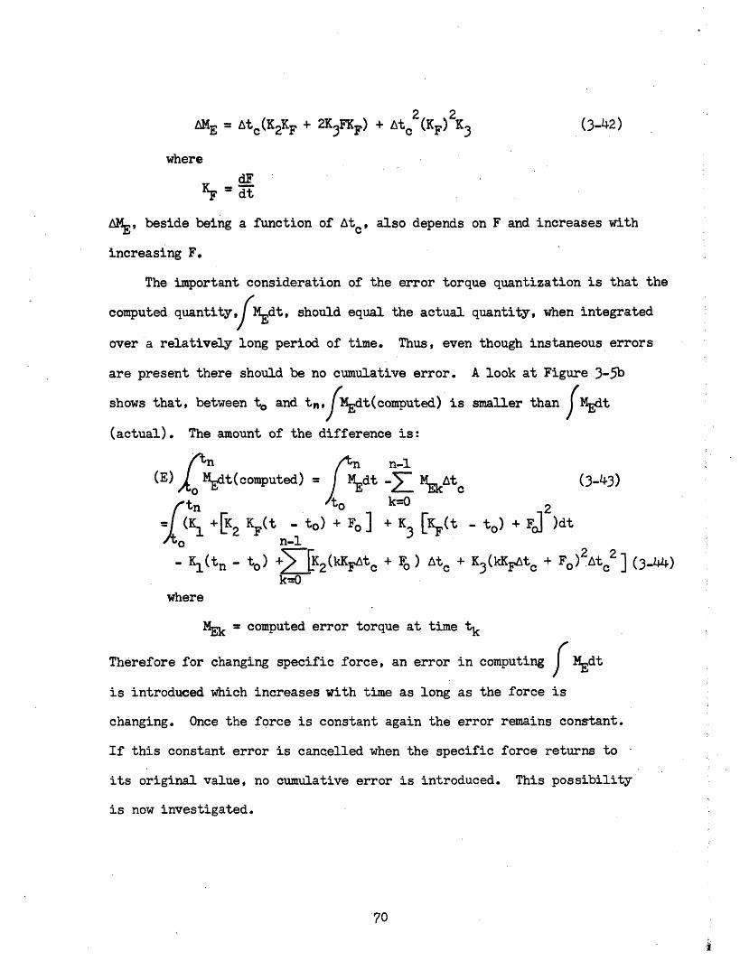
ME = Atc(K2KF + 2K3 FKF ) + tc (KF) K3 (3-42)
where
dFF = dt
AME, beside being a function of Ate, also depends on F and increases with
increasing F.
The important consideration of the error torque quantization is that the
computed quantity.f dt, should equal the actual quantity, when integrated
over a relatively long period of time. Thus, even though instaneous errors
are present there should be no cumulative error. A look at Figure 3-5b
shows that, between t and tn. dt(comuted) is smaller than MEdt
(actual). The amount of the difference is:
( n n-l
(E) dt(computed) -t 7k Atc (3-43)
tn k=O
4K1 +[K2 KF(t -t o ) + F + K3 KF(t - to ) + Fj 2dto n-l
- (tn t) + K2(kKFAtc + Fo) Atc + K3(kKFtc + Fo)2 Atc ] (3-44)k--
where
MEk= computed error torque at time tk
Therefore for changing specific force, an error in computing f Mdtis introduced which increases with time as long as the force is
changing. Once the force is constant again the error remains constant.
If this constant error is cancelled when the specific force returns to
its original value, no cumulative error is introduced. This possibility
is now investigated.
70
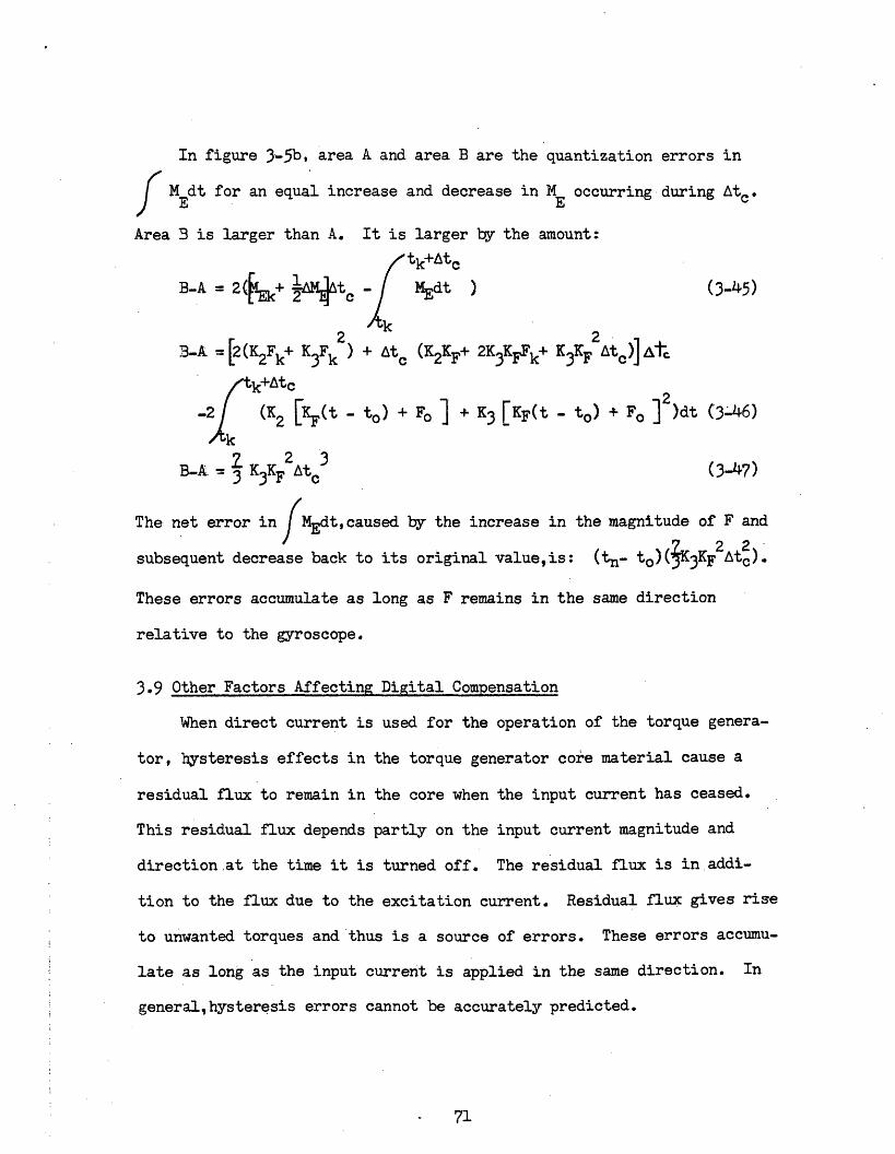
In figure 3-5b, area A and area B are the quantization errors in
ME dt for an equal increase and decrease in ME occurring during Atc .
Area 3 is larger than A. It is larger by the amount:
tk+AtC
B-A = 2( + t - MEdt )(3-45)
Ftc 22 3tk+Atc
B-A- 3 K3KF Atc (3-7)
The net error in fMEdt,caused by the increase in the magnitude of F and
subsequent decrease back to its original value,is: (tn- to)( 3KF Atc).
These errors accumulate as long as F remains in the same direction
relative to the gyroscope.
3.9 Other Factors Affecting Digital Compensation
When direct current is used for the operation of the torque genera-
tor, hysteresis effects in the torque generator core material cause a
residual flux to remain in the core when the input current has ceased.
This residual flux depends partly on the input current magnitude and
direction at the time it is turned off. The residual flux is in addi-
tion to the flux due to the excitation current. Residual flux gives rise
to unwanted torques and thus is a source of errors. These errors accumu-
late as long as the input current is applied in the same direction. In
general,hysteresis errors cannot be accurately predicted.
71
When alternating current is used for operation of the torque genera-
tor, the mmf due to the excitation current is alternating and therefore
constantly recycling the hysteresis loop. Residual flux is then no longer
a problem. A residual flux problem does occur with alternating current,
however, when an input current is suddenly applied whose mmf is approxi-
mately equal to the excitation mmf. Under these conditions the net mmf
at two of the torque generator poles is very low. Any residual flux may
then be large compared to the alternating component. This problem can
be eliminated by keeping the input and excitation mmf's sufficiently
different in amplitude.
The stability of the source supplying torque generator current is
important because of its effect on the torque produced by the torque
generator. If the same source supplies both input and excitation cur-
rents, a small fluctuation in the source voltage causes a percentage
fluctuation in torque approximately twice as great, since the torque is
proportional to the product of the currents.
Torque generator input current-torque non-linearities caused by norn-
linearities of the core material do not effect torque control methods
2, 3 and 4, since the compensation torque magnitude is constant for
these methods. It is only necessary to initially calibrate the torque
at the level used. Method 1 is effected by torque generator non-linearities,
since torque level changes occur. These effects can also be overcome,
however, by adjusting each individual torque level.
72
Chapter IV
DIGITAL COMPENSATION TESTS
4.1 Introduction
In order to determine the actual errors present in a digital com-
pensation system, a test setup was constructed. A series 10.0 FG-1-2
floated gyroscope was used for the tests. The gyroscope was mounted on
a Griswold rotary table with its output axis coincident with the table
axis and perpendicular to the local gravity vector. The gyroscope
could thus be rotated about its output axis and its angular position
accurately determined by a magnified vernier dial on the rotary table.
Oriented in this way, compliances and the mass unbalance about the
gyroscope output axis cause a torque to act on the torque summing mem-
ber due to gravity. Since the position of the gyroscope relative to
gravity could be changed by rotating the table, the magnitude and
direction of the error torque could be varied. No stabilization servu
was used with the gyroscope for reasons stated before. Since the servo
was omitted, the gyro wheel did not have to be running. This in turn
eliminated the need to cancel out any precession of the gyro wheel due
to earth rate.
A block diagram of the test setup used appears in Figure 4-1.
This setup was modified for different tests. The intention was not to
73
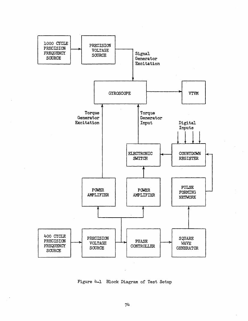
SignalGeneratorExcitation
PGYROSCOPE
TorqueGeneratorExcitation
TorqueGeneratorInput
4-
Figure 4-1 Block Diagram of Test Setup
74
1000 CYCLEPRECISIONFREQUENCYSOURCE
PRECISIONVOLTAGESOURCE
VTVM
DigitalInputs
111 1
ELECTRONICSWITCH
COUNTDOWNREGISTER
POWERAMPLIFIER
POWERAMPLIFIER
PULSEFORMINGNETWORK
400 CYCLEPRECISIONFREQUENCYSOURCE
PRECISIONVOLTAGESOURCE
PHASECONTROLLER
SQUAREVWAVE
GENERATOR
_ !
! ! ! =
--
r rj
l
. .--
jI
_I I__
test a complete digital compensation system, since such a test would have
necessitated having practically a complete inertial system. A countdown
register was used, into which simulated digital computer outputs were fed.
Clock pulses were obtained from a square wave derived from the 400 cycle
torque generator current. These clock pulses were also used for timing
when direct current was used for the torque generator. Both the frequency
and amplitude of the torque generator and signal generator currents were
precisely controlled. Torque summing member angular position was determined
by a V. T. V. M. which monitored the gyroscope signal generator output
voltage.
Designing an adequate electronic switch for the tests proved some-
what difficult. The difficulty encountered is that since a transistor is
a three terminal device, no possibility exists of isolating the circuit
that controls the transistor from the circuit the transistor controls.
The electronic switch uses direct current signals to switch alternating
current. Relays possess the four terminal operation needed, but are
limited by their slow switching characteristics. At first a circuit using
four switching transistors in a demodulator-type circuit was tried.
Problems were encountered with the alternating current shorting through
one-half of the switch on alternate half cycles. This was caused by
collector-base conduction in the switching transistors. The circuit
finally used is shown in Figure 4-2. Only two transistors are used for the
actual switching. When either of the switching transistors is cut off,
75
To o400 Cycle o
Power o°Supply C
0
2N1122A
0.
1.8
Input
(-0v, 0)
que
tornding
v
° Input
(0, -10v)
10
To -10v
Resistors in k
Condensers in Eif
Figure 4-2 Schematic Diagram of Electronic Switch
76
IL
its base is biased at a voltage higher than the peak alternating current
voltage that appears at the collector. Therefore collector-base conduction
is prevented.
The test setup outlined above was first used to determine to what
extent certain of the errors discussed in Chapter III affected an actual
system. Then, tests were run to see how well the torque control methods
described in Chapter II performed.
4.2 Test Methods
A plot of gyroscope unbalance torque as a function of rotary table
angular position was first obtained. The torque, for one degree in-
crements of table position, was determined by measuring the torque gen-
erator currents required to hold the torque summing member at null for
a certain period of time and using available data on torque generator
sensitivity. Using this plot, a table angular position could be chosen
to obtain a certain unbalance torque about the gyroscope output axis.
Likewise an effective torque generator torque could be measured by setting
the table at a position that resulted in zero drift of the torque summing
member. The curve obtained was correct only when the torque summing mem-
ber was at null. However, by restricting movements of the torque summng
member to approximately 0.1 milliradian either side of null, essentially
constant torques were obtained while allowing movements of the torque
summing member for purposes of viscous shear integration.
In the following discussion the unit of torque used is meru. Meru,
77
or milli-earth-rate-unit,is not a torque unit, but an angular rate unit.
However, for any given gyro wheel angular momentum, a constant angular
rate input to a gyroscope will produce a certain torque about the output
axis. A 1 meru torque, therefore, is a torque equal to that produced by
a 1 meru input to the gyroscope under consideration.
The drift rate measurements taken during the tests described here
were obtained as follows. The reading of the V. T. V. M. monitoring the
gyroscope signal generator output was related to the torque summing mem-
ber position by the signal generator sensitivity. The amount of time
for drift of the torque summing member to cause a certain change in meter
reading was measured by a manually operated electric timer. A large
magnifying glass was used to help determine the meter indications. The
drift measurements thus obtained were average rates over the times of
observation. The accuracy of the drift measurements was probably deter-
mined by the accuracy of the V. T. V. M. and the accuracy of relative
drift measurements by the repeatability of the instrument.
4.3 Tests and Results
Test 1 - Effects of Non-Newtonian Damning Fluid, Non-Laminar Flow and
Suspension Friction
The following tests were performed to determine any effects caused
by non-Newtonian characteristics or non-laminar flow of the gyroscope
damping fluid. The tests consisted of setting the position of the
rotary table to obtain, for separate tests, three different unbalance
78
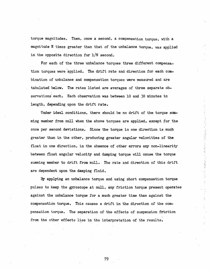
torque magnitudes. Then, once a second, a compensation torque, with a
magnitude N times greater than that of the unbalance torque, was applied
in the opposite direction for 1/N second.
For each of the three unbalance torques three different compensa-
tion torques were applied. The drift rate and direction for each com-
bination of unbalance and compensation torques were measured and are
tabulated below. The rates listed are averages of three separate ob-
servations each. Each observation was between 10 and 30 minutes in
length, depending upon the drift rate.
Under ideal conditions, there should be no drift of the torque sum-
ming member from null when the above torques are applied, except for the
once per second deviations. Since the torque in one direction is much
greater than in the other, producing greater angular velocities of the
float in one direction, in the absence of other errors any non-linearity
between float angular velocity and damping torque will cause the torque
summing member to drift from null. The rate and direction of this drift
are dependent upon the damping fluid.
By applying an unbalance torque and using short compensation torque
pulses to keep the gyroscope at null, any friction torque present operates
against the unbalance torque for a much greater time than against the
compensation torque. This causes a drift in the direction of the com-
pensation torque. The separation of the effects of suspension friction
from the other effects lies in the interpretation of the results.
79
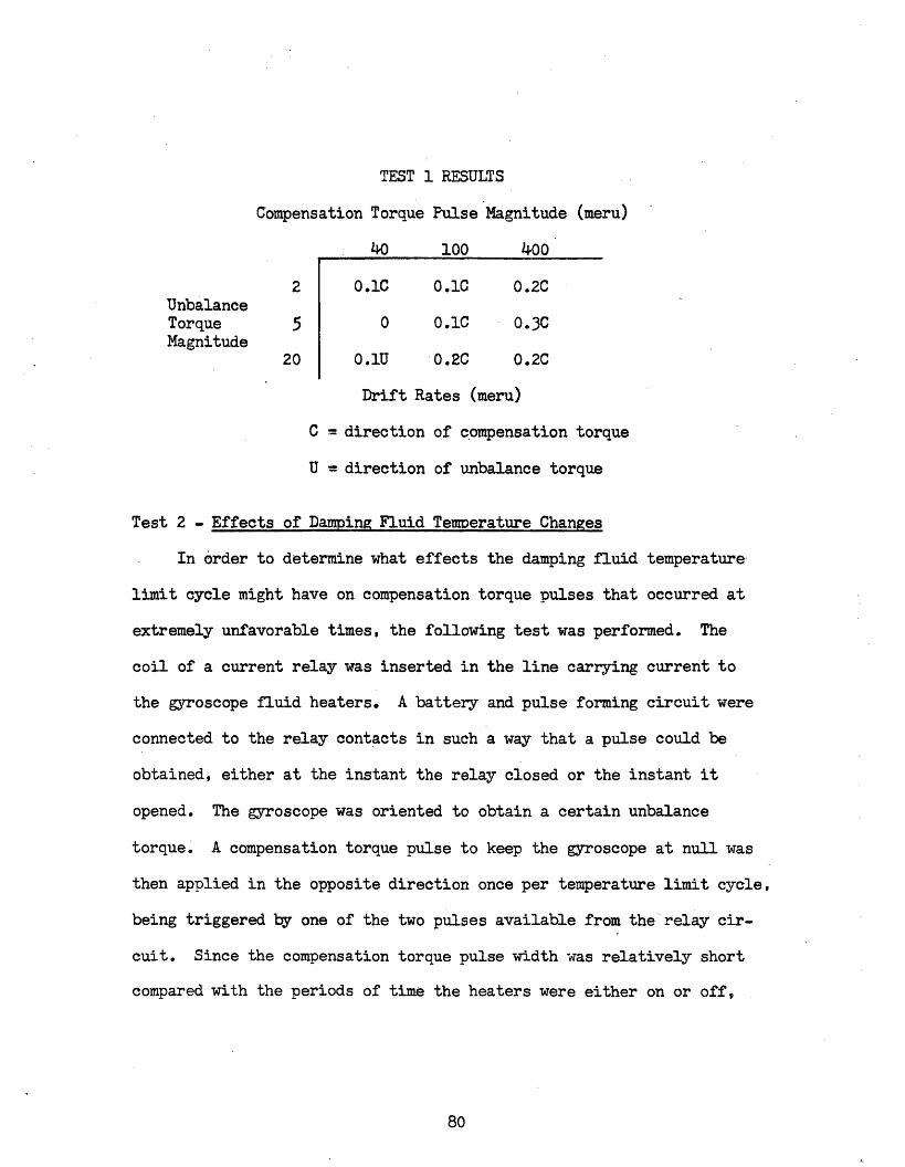
TEST 1 RESULTS
Compensation Torque Pulse Magnitude (meru)
40 100 400
UnbalanceTorqueMagnitude
2
20
0.1C 0.1C 0.2C
0 0.1C 0.3C
0.1U -0.2C 0.2C
Drift Rates (meru)
C = direction of compensation torque
U = direction of unbalance torque
Test 2 - Effects of Damping Fluid Temverature Changes
In order to determine what effects the damping fluid temperature
limit cycle might have on compensation torque pulses that occurred at
extremely unfavorable times, the following test was performed. The
coil of a current relay was inserted in the line carrying current to
the gyroscope fluid heaters. A battery and pulse forming circuit were
connected to the relay contacts in such a way that a pulse could be
obtained, either at the instant the relay closed or the instant it
opened. The gyroscope was oriented to obtain a certain unbalance
torque. A compensation torque pulse to keep the gyroscope at null was
then applied in the opposite direction once per temperature limit cycle,
being triggered by one of the two pulses available from the'relay cir-
cuit. Since the compensation torque pulse width was relatively short
compared with the periods of time the heaters were either on or off,
80
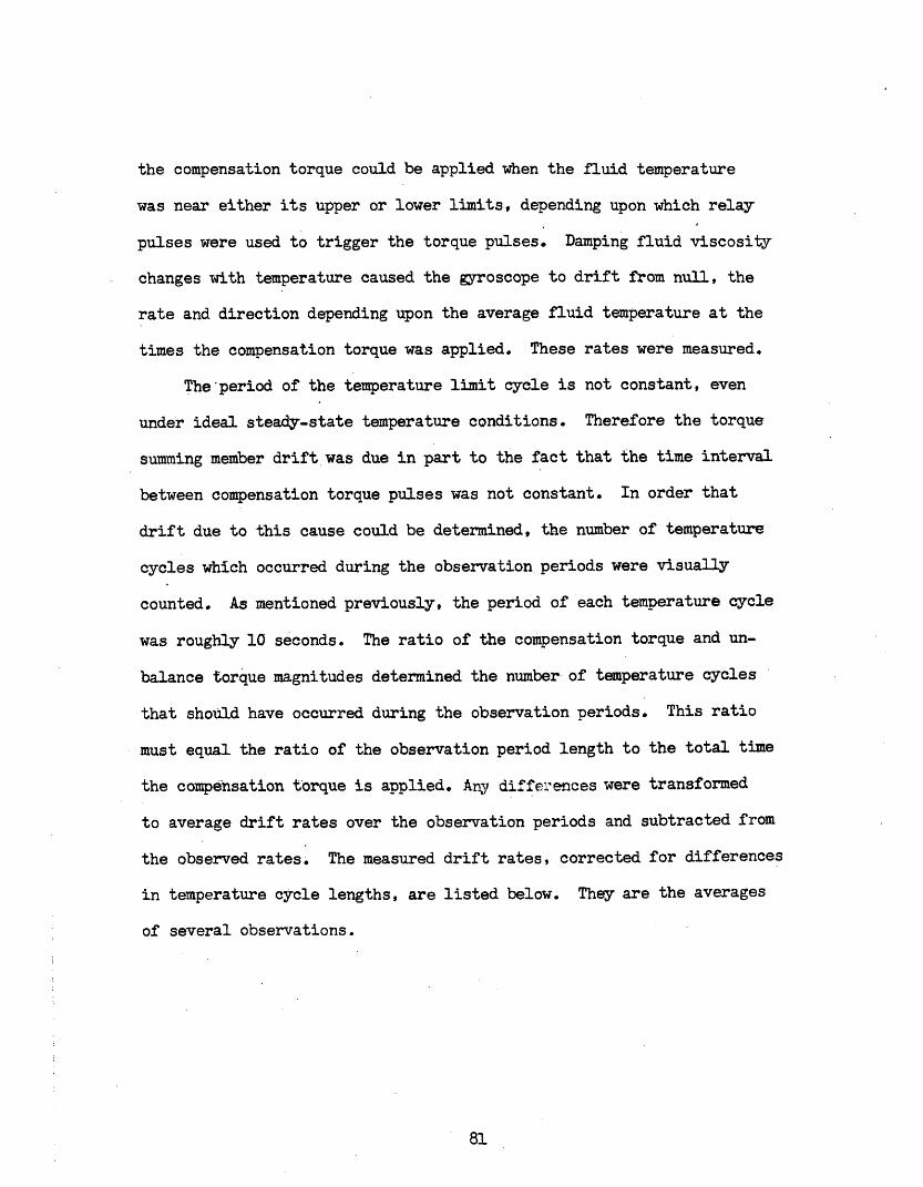
the compensation torque could be applied when the fluid temperature
was near either its upper or lower limits, depending upon which relay
pulses were used to trigger the torque pulses. Damping fluid viscosity
changes with temperature caused the gyroscope to drift from null, the
rate and direction depending upon the average fluid temperature at the
times the compensation torque was applied. These rates were measured.
The period of the temperature limit cycle is not constant, even
under ideal steady-state temperature conditions. Therefore the torque
summing member drift was due in part to the fact that the time interval
between compensation torque pulses was not constant. In order that
drift due to this cause could be determined, the number of temperature
cycles which occurred during the observation periods were visually
counted. As mentioned previously, the period of each temperature cycle
was roughly 10 seconds. The ratio of the compensation torque and un-
balance torque magnitudes determined the number of temperature cycles
that should have occurred during the observation periods. This ratio
must equal the ratio of the observation period length to the total time
the compensation torque is applied. Any differiences were transformed
to average drift rates over the observation periods and subtracted from
the observed rates. The measured drift rates, corrected for differences
in temperature cycle lengths, are listed below. They are the averages
of several observations.
81
TEST 2 RESULTS
Unbalance PulseTorque Width Fluid DriftMagnitude (sec.) Temperature Rates
20 0.25 high 0.3C
20 0.25 low 0.2U
50 0.50 high 0.7C
50 0.50 low 0.6u
Test 3 - Switching Transient Effects
The effects of torque generator input current transients due to
switching were next determined. As before, compensation torque pulses
were used to cancel the effects of an unbalance torque on the torque
summing member. When alternating current was used on the torque
generator windings, the pulses used were one cycle in width and the
timing of the clock pulses controlling the switching was varied in order
to vary the phase angle of the current when it was switched. In this
way, the effects of transients caused by switching not taking place at
the proper phase angle could be determined by measuring any gyroscope
drifting produced.
WThen direct current was used on the torque generator windings, the
effects of transients were determined by varying the length of the com-
pensation torque pulses used. If the unbalance torque magnitude is
varied in direct proportion to the compensation torque pulse length,
82
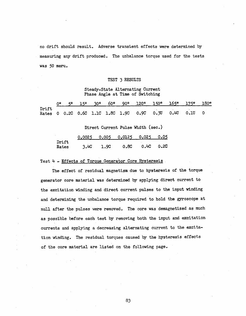
no drift should result. Adverse transient effects were determined by
measuring any drift produced. The unbalance torque used for the tests
was 50 meru.
TEST 3 RESULTS
Steady-State Alternating CurrentPhase Angle at Time of Switching
00 50 15° 30Q 600 900 120° 150° 165° 175° 180°DriftRates 0 0.2C 0.6C 1.lC 1.8C 1.9C 0.9C 0.3U 0.4U O.1U 0
Direct Current Pulse Width (sec.)
0.0025 0.005 0.0125 0.025 0.05DriftRates 3.4C 1.90C 0.4C 0.2C
Test 4 - Effects of Torque Generator Core Hysteresis
The effect of residual magnetism due to hysteresis of the torque
generator core material was determined by applying direct current to
the excitation winding and direct current pulses to the input winding
and determining the unbalance torque required to hold the gyroscope at
null after the pulses were removed. The core was demagnetized as much
as possible before each test by removing both the input and excitation
currents and applying a decreasing alternating current to the excita-
tion winding. The residual torques caused by the hysteresis effects
of the core material are listed on the following page.
83
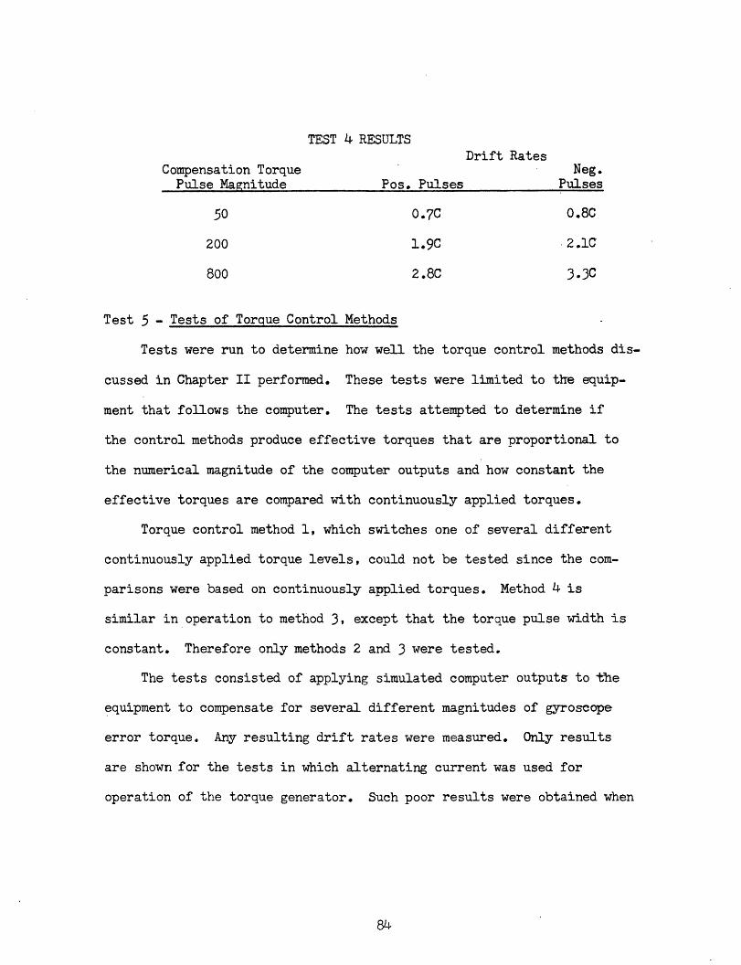
TEST 4 RESULTS
Drift RatesCompensation Torque Neg.
Pulse Magnitude Pos. Pulses Pulses
50 0.7C 0.8C
200 1.9C 2.1C
800 2.8C 3.3C
Test 5 - Tests of Torque Control Methods
Tests were run to determine how well the torque control methods dis-
cussed in Chapter II performed. These tests were limited to the equip-
ment that follows the computer. The tests attempted to determine if
the control methods produce effective torques that are proportional to
the numerical magnitude of the computer outputs and how constant the
effective torques are compared with continuously applied torques.
Torque control method 1, which switches one of several different
continuously applied torque levels, could not be tested since the com-
parisons were based on continuously applied torques. Method 4 is
similar in operation to method 3, except that the torque pulse width is
constant. Therefore only methods 2 and 3 were tested.
The tests consisted of applying simulated computer outputs to the
equipment to compensate for several different magnitudes of gyroscope
error torque. Any resulting drift rates were measured. Only results
are shown for the tests in which alternating current was used for
operation of the torque generator. Such poor results were obtained when
84
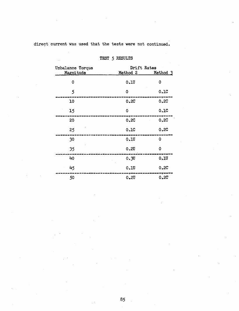
direct current was used that the tests were not continued.
TEST 5 RESULTS
Unbalance TorqueMagnitude
0
5
10
15
Drift RatesMethod 2 Method 3
0O.1U
0
0.2C
0
20
25
30
35
40
45
5o0
0.1C
0,2C
0.1C
0.2C
0.1C
0.1U
0.2U
0.2C
0.2C
0
0
0.3U
0.1U
0.2U
0.1U
0.2C
0.2C
85

06
ChaDter V
CONCLUSIONS
5.1 Discussion of Test Results
Test 1 - The results of Test 1 are inconclusive to some extent.
While most of the measurements seem to indicate the presence of friction
torques, some of the individual measurements taken were completely op-
posite of what they should have been under such circumstances. The re-
sults seem to indicate a friction torque equivalent to between 0.1 and
0.2 meru. For the gyroscope used this would correspond to roughly 0.1
dyne-cm.
Effects of non-Newtonian damping fluid or non-laminar flow, which
would probably be indicated by drifts in the direction of the unbalance
torque, i. e., b greater than 1, did not seem to be present. Even the
greatest float angular velocities encountered were probably much less
than would be needed to reach non-laminar flow conditions. Also, the
damping fluid is very carefully chosen to exhibit pure Newtonian
qualities. Therefore any effects due to these causes were probably
either in the same range or below the accuracy of the equipment and
methods used for the tests.
Test 2 - The results' of Test 2 were approximately as anticipated.
The compensation torque pulses applied when the damping fluid tempera-
ture was near its upper limit caused the torque summing member to drift
in the direction of the compensation toraue. -Wihen the pulses were applied while
the daming fluid temperature was near its lower limit a drift was caused
87
in the direction of the unbalance torque. The drift rates were somewhat
larger than would have been predicted by considerations discussed in
Chapter III. This may have been due to the temperature control limits
being different than specified. Also the fact that the fluid heaters
and temperature controller are physically separated in the gyroscope
may allow wider temperature excursions of the damping fluid in the
vicinity of the heaters or other fluid areas remote from the controller.
The compensation torque pulses used in Test 2 were applied at ex-
tremely unfavorable times. The chances of such pulse timing occurring
in actual operation, except for short periods, are very remote. However,
the chances of having a completely symmetrical distribution of torque
pulses over the fluid temperature range is also remote. Therefore damping
fluid temperature variations probably have some effect on digital drift
compensation.
Test 3 - Test 3 shows that torque generator current transients can
definitely affect digital drift compensation. The results of switching
alternating input current when the steady-state current was at a rela-
tively high value produced large drift rates. These drift rates were
greatly reduced when the steady current wave was close to zero at the
time of switching. The current pulses used for Test 3 were one cycle
in width. Since the transients occur only on the ends of the pulses,
as the pulse width is increased to a greater number of cycles the drift
rate would be expected to be reduced by a factor of approximately the
number of cycles. This proved to be the case in tests involving
88
larger numbers of cycles.
The results of using direct current pulses on the torque generator
input winding shows that transients greatly affect the torque produced
in such a case. As the pulse length was increased, decreasing the
relative effects of the transients, the drift rates decreased almost
proportionately. Unfortunately, when using direct current, there is
no simple way of reducing the transients as there is for the alternating
current case.
Test 4 - Torque generator residual magnetism caused by core material
hysteresis effects produces residual torques when direct current excita-
tion is used, as the results of Test 4 show. These residual torques
cause drifting of the torque summing member and are definitely unde-
sirable for digital drift compensation. Tests using alternating current
on the torque generator windings showed no apparent residual torques
caused by hysteresis effects.
Test 5 - The results of Test 5 indicate that the torque control
methods used produce linear torque control and constant torques to a
certain degree. This degree may be largely due to uncertainties in
the measurements. The repeatability of the unbalance torques is some-
what in question. While the rotary table angle could be repeated with
good accuracy, causes such as torque summing member mass shift due to
bearing play and other uncertainties produced repeatability errors in
the unbalance torques. The stability of the power supplies and other
equipment used was also a factor. The drift torque rates observed may
89
have been of the order of magnitude of the uncertainty torques of the
gyroscope used. Factors already mentioned such as suspension friction
and damping fluid temperature changes may also have added to the drifts
observed. The phase splitting transformer used did not produce exactly
equal voltages on each side of the center tap. This is one reason the
zero torque level as well as other torque levels of Method 2 produced
drifts.
Since unbalance constants supplied with the gyroscope had an ac-
curacy of only 0.1 meru, the results of Test 5 are probably as good as
they need be for the compensation of the particular gyroscope used.
5.2 Conclusions
Drift compensation of a gyroscope with the use of digital informa-
tion can be accomplished by several different methods. For many reasons
these methods cannot cancel out the instantaneous error torque producing
drift. They can, however, cancel out the long term effects of the error
torque. The cancelling of these effects depends upon the integrating
properties of the gyroscope. Thus digital controlled compensation
differs from the normal method of drift compensation, which ideally can
cancel out the instantaneous error torque and therefore does not rely
heavily on integration by the gyroscope torque summing member. Certain
factors cause the integration process in gyroscopes to be imperfect.
Due to the extreme care used in making gyroscopes, these imperfections
are quite small. They therefore do not appear to limit the usefulness
of digital controlled drift compensation.
90
Some factors should receive special attention when drift compensa-
tion is digital controlled. They are as follows:
1. The maximum angular excursions of the torque summing
member, caused by differences of the applied compensation torque from
the ideal, should be less than the resolution of the gyroscope stabili-
zation servo.
2. When digital accelerometers, such as the type discussed
in Chapter III, are used to obtain the specific force data, the itera-
tion time of the error torque digital computations depends upon the
specific force profile to be experienced by the inertial system. If
the system experiences frequent changes in specific force, the itera-
tion time should be relatively short in order to reduce compensation
torque quantization errors. If the system experiences infrequent
changes in specific force, the iteration time should be relatively
long in order to obtain more accurate specific force data.
3. The gyroscope damping fluid temperature should be main-
tained as constant as possible.
4. Only alternating currents should be used for the operation
of the gyroscope torque generator. Switching transients and core
material hysteresis effects cause direct current to be extremely unde-
sirable for such use. In order to reduce transients, the alternating
current should be switched only when the steady-state current wave
passes through zero. To reduce the effects of any transients, the
current pulses should contain only complete cycles and the shortest
91
pulse used should contain several cycles.
5. To reduce the effects of cross-coupling currents, the.
torque generator power supply should have a high output impedance.
5.3 Recommendations for Further Study
1. Work could be done on determining a method of calculating the
error torque which would not necessitate a compromise in the iteration
time for the desired results of low quantization error and high in-
stantaneous torque determination accuracy.
2. A more accurate determination of the actual effects of the
sources of error mentioned in Chapter III could be accomplished. This
would probably require a more elaborate setup than was used for this
thesis, utilizing better equipment and methods.
3. Work could be done on a method of digital torque control which
operates by changing the phase angle btween the torque generator ex-
citation and input currents.
92
BIBLIOGRAPHY
1. Gianoukos, W. A., and Palmer, P. J., Gyro Test Laboratory Unbalance
Equations, Report GT-130, MIT Instrumentation Laboratory, 1960.
2. Denhard, W. G., Laboratory Testing of a Floated, Single-Degreeof-
Freedom, Integrating Inertial Gyro, Report R-105, MIT Instrumentation
Laboratory, 1956.
3. Draper, C. S., Wrigley, W., and Grohe, L. R., The Floating Integrating
Gyro and Its Application To Geometrical Stabilization Problems on
Moving Bases, Institute of Aeronautical Sciences, 1955.
4. Gilinson, P. J., Jr., and Hofmann, G., Optimum Control of
Instrument Output Axis Torque Inaccuracies, Report T-15, MIT
Instrumentation Laboratory, 1952.
5. MIT Instrumentation Laboratory, The Spire, Jr. Long Range Inertial
Guidance System, Report R-193, Final Engineering Report, 1959, SECRET.
6. Gauntt, F. E., Digitally Controlled Pulse Torquing of Precision
Inertial Instruments, Report E-638, MIT Instrumentation Laboratory,
1957.
7, Cohen, A. R., A Design of a Practical Digital Accelerometer System,
Master's Thesis, MIT Instrumentation Laboratory, 1958, CONFIDENTIAL.
8. Lees, Sidney, Integration by the Viscous Shear Process,
Report 6398-T-10, MIT Instrumentation Laboratory, 1950.
9. Mueller, R. K., Microsyn Electromagnetic Components, MIT Instrumentation
Laboratory, 1952.
93