i

Faculty of Science and Technology

MASTER’S THESIS

Study program/ Specialization:

Master of Science in Petroleum Engineering

Drilling and Well Technology

Spring semester, 2012

Restricted access

Writer:

Joar Grimsrud

………………………………………… (Writer’s signature)

Faculty supervisor:

Bernt Sigve Aadnøy

External supervisor(s):

Roy Marker, Statoil ASA

Cecilie Dyrkorn, Statoil ASA

Titel of thesis:

Deepwater Operations – Running and Cementing Casing with Small Clearances

Credits (ECTS): 30

Key words:

Deepwater Drilling

Low Clearances

Running Casing

Cemening

Pages: 96

+ enclosure: 8

Stavanger, 15th

of June, 2012

ii

Abstract

The petroleum demand is increasing and the line between success and failure is marginal. Thus, the drilling

industry moves further into deeper waters, stretching the limits of engineering, economics and new

technology to the maximum.

A natural consequence of increasing water depths is the decreasing operational window. This is due to the fact

that rock is being replaced by seawater, and the resulting overburden gradient is reduced. If the pore pressure

is held equal to the hydrostatic gradient of water, the decreasing operational window is evident.

The consequences of this in deepwater operations are generally a more complex casing design and increased

risk for well control incidents. This thesis takes an in-depth analysis of the as is situation in deepwater drilling

today, with an especial focus on the low clearances between the casings and liners. Five wells from Gulf of

Mexico (GoM) and Egypt deepwater environments are reviewed. The 13 5/8” section of each section is

especially evaluated in terms of running and cementing casing. A pre and post study technique is used to

evaluate plan against what actually happened.

Simultaneously throughout the thesis, a fictive well, Well 1, is built and used. Well 1 is based on a GoM well

and is used to perform simulations in comparison to the five deepwater wells. Well 1 is further analysed in

terms of potential solutions and mitigating technologies.

Several potential solutions or mitigating technologies are found. These are:

Dual gradient drilling

Managed pressure drilling, MPD

Casing drilling

Liner drilling

Low ECD fluids

Furthermore, combined potential solutions were found:

Combined MPD and dual gradient drilling

Liner drilling combined with expandable liners

These are currently under development.

iii

Acknowledgements

This master thesis concludes five years of study at University of Stavanger, UiS. The study program is Master

of Sience in Petroleum Engineering, Drilling and Well Technology.

The thesis is written for UiS, in cooperation with Statoil ASA, Stavanger. The target audience of this thesis is

assumed to have basic technical drilling and well background.

First of all, I would like to thank my supervisors, Bernt Sigve Aadnøy (UiS), Roy Marker (Statoil ASA) and

Cecilie Dyrkorn (Statoil ASA) for input and proposals in how to approach my work on deepwater operations.

I would also like to thank Tor Henry Omland, Ben Watts, Kjetil Bekkeheien, Siddhartha Lunkad, Dag Ove

Molde and Gaute Grindhaug in the Statoil ASA for always taking the time to answer my questions.

I would also like to thank my fellow student, Bernt-Andrè Lorentsen, for constructive discussion and inputs

over the last semester.

Finally, I would like to thank my fiancé, Lina, and son, Fillip for being so patient and understanding

throughout my studies at UiS.

Joar Grimsrud

iv

Table of Contents

Abstract ............................................................................................................................................................... ii

Table of Contents ............................................................................................................................................... iv

List of Figures .................................................................................................................................................... vi

List of Tables ..................................................................................................................................................... ix

Introduction ..................................................................................................................................................1 1

Deepwater Drilling .......................................................................................................................................2 2

Background ..........................................................................................................................................2 2.1

Well 1 ...................................................................................................................................................3 2.2

Validity of Well 1 ................................................................................................................................6 2.3

Deepwater Drilling Operations ............................................................................................................7 2.4

Well Integrity .............................................................................................................................................12 3

Normalization of data.................................................................................................................................15 4

Drilling Fluids ............................................................................................................................................17 5

Rheology ............................................................................................................................................17 5.1

Rheological models ....................................................................................................................17 5.1.1

Water Based Mud ..............................................................................................................................19 5.2

Oil Based Mud ...................................................................................................................................19 5.3

Synthetic Based Mud .........................................................................................................................20 5.4

Drilling Fluid Fundamentals ..............................................................................................................20 5.5

Drilling Fluid Functions .............................................................................................................20 5.5.1

Mud System ...............................................................................................................................21 5.5.2

Cementing ..................................................................................................................................................22 6

Washers and Spacers ..........................................................................................................................22 6.1

Cement and Cement Additives ..........................................................................................................22 6.2

Lightweight and Ultralow-Density Cements System .........................................................................24 6.3

Cement and Additive Equipment .......................................................................................................26 6.4

Casing Hardware Tools ......................................................................................................................28 6.5

Casing Shoe ...............................................................................................................................28 6.5.1

Surge Reduction Tools ...............................................................................................................29 6.5.2

Plugs ...........................................................................................................................................32 6.5.3

v

Stage Cementing ........................................................................................................................35 6.5.4

Centralizers ................................................................................................................................35 6.5.5

Wellbore Preparations ........................................................................................................................37 6.6

Cement Job .........................................................................................................................................37 6.7

Cement Testing ..................................................................................................................................38 6.8

Consequenses of a Poor Cement Job .................................................................................................38 6.9

Requirements .............................................................................................................................................40 7

Drilling Fluid Requirements ..............................................................................................................40 7.1

Cementing Requirements ...................................................................................................................40 7.2

Hydraulic Simulator ...................................................................................................................................42 8

Surge Module .....................................................................................................................................42 8.1

Cementing Module .............................................................................................................................43 8.2

Case ............................................................................................................................................................44 9

Well 1 .................................................................................................................................................44 9.1

Simulations Basis .......................................................................................................................47 9.1.1

Simulations – Running 13 5/8” Casing ......................................................................................47 9.1.2

Simulations - Cementing 13 5/8” Casing ...................................................................................57 9.1.3

GoM and Egypt Deepwater Wells .....................................................................................................62 9.2

Well A ........................................................................................................................................63 9.2.1

Well B ........................................................................................................................................66 9.2.2

Well C ........................................................................................................................................69 9.2.3

Well D ........................................................................................................................................71 9.2.4

Well E ........................................................................................................................................74 9.2.5

Economical Aspect ............................................................................................................................76 9.3

Potential Solutions .................................................................................................................................77 10

Dual Gradient Drilling .......................................................................................................................77 10.1

MPD ...................................................................................................................................................82 10.2

Microflux™ Control Method and Ultralow Invasion Fluid .......................................................84 10.2.1

Casing and Liner Drilling ..................................................................................................................85 10.3

Low ECD Fluids ................................................................................................................................87 10.4

Conclusions ............................................................................................................................................90 11

Abbreviations .....................................................................................................................................................91

References ..........................................................................................................................................................92

Appendix A –Simulation Input Data Well 1 ........................................................................................................ I

vi

List of Figures

Figure 2.1: Hydrostatic gradient and overburden gradient seen at increased (from right to left) water depths ...2

Figure 2.2: Hydrate formation curve showing pressure at y-axis and temperature on x-axis (Janssen, 2011) ....3

Figure 2.3: Setup Well 1. Based on figure from Bureau of Ocean Energy Management, Regulation and

Enforcement (BOEMRE) – Subsalt Exploration .................................................................................................5

Figure 2.4: Pressure gradient plot for Well 1 .......................................................................................................5

Figure 2.5: Well A, GoM (Statoil, 2012) .............................................................................................................6

Figure 2.6: Expected pore pressure plot, Well A (Statoil, 2012) .........................................................................7

Figure 2.7: Discoverer Americas ©Transocean Ltd. ...........................................................................................8

Figure 2.8: Maersk Developer © Maersk Drilling ...............................................................................................8

Figure 2.9: Pressure gradient plot from the Statfjord field. Note that units are in [m] and [sg]. .........................9

Figure 2.10: Mud program with casing setting depths for well 1 in order to reach target depth. Note that units

are in [ft] and [ppg]. .............................................................................................................................................9

Figure 2.11: RMR™ system from AGR Drilling Services (Newswise, 2009) ..................................................10

Figure 2.12: Rhino Reamer© from Schlumberger (Schlumberger, 2012) .........................................................10

Figure 2.13: Typical casing program for a well at the Statfjord field versus Well 1. ........................................11

Figure 3.1: Example of wellbore stresses (Aadnøy, 2010) ................................................................................13

Figure 3.2: Graphic modeling of pipe being tripped into hole (Nelson, et al., 2006) ........................................14

Figure 4.1: Semi-submersible versus drillship. Figure based on figure from Wikipedia (Wikipedia, 2012). ...15

Figure 5.1: Fluids of different rheological characters (Romanian Society of Rheology, 2011) ........................17

Figure 5.2: Different Newtonian and non-Newtonian rheological models (Nelson, et al., 2006) .....................19

Figure 5.3: Mud circulation system ...................................................................................................................21

Figure 6.1: by adding a surfactant two immiscible fluids can go from scenario A to D (Wikipedia, 2012) .....22

Figure 6.2: Cement manufacturing process (CEMEX, 2011) ............................................................................23

Figure 6.3: Hot clinker after heating process (Wikipedia, 2008) .......................................................................23

Figure 6.4: Foam cement cloes-up (Huatai, 2012) .............................................................................................25

Figure 6.5: Displacement tank (Nelson, et al., 2006).........................................................................................27

Figure 6.6: Metering Rack with smart valves (Nelson, et al., 2006) .................................................................27

Figure 6.7: Jet mixer (Nelson, et al., 2006) ........................................................................................................28

Figure 6.8: Guide shoe (left) float shoe (right) with double float valve setup (Nelson, et al., 2006) ................29

Figure 6.9: Various setup used when running casing (Nelson, et al., 2006) ......................................................30

Figure 6.10: Conversion from autofill to float (A to D) (Nelson, et al., 2006) ..................................................30

Figure 6.11: Diverter, Surgemaster II™, from Weatherford (Nelson, et al., 2006) ...........................................31

Figure 6.12: Typical Surgemaster II™ Running Envelope (Statoil, 2012) ......................................................32

Figure 6.13: Top and bottom plug (Nelson, et al., 2006) ..................................................................................33

Figure 6.14: Plugs with anti-rotation feature (Nelson, et al., 2006) ..................................................................33

Figure 6.15: subsea cementing system with typical setup seen both on rig floor (top) and seabed (bottom)

(Nelson, et al., 2006) ..........................................................................................................................................34

Figure 6.16: Subsea wiper plug system illustrating both plugs and darts (Nelson, et al., 2006) .......................34

Figure 6.17: Indicator collar (bottom) with constriction in the middle. Plug at top (Weatherford, 2012) .........34

Figure 6.18: Hydraulic stage tool (Nelson, et al., 2006) ...................................................................................35

Figure 6.19: Velocity profiles at various eccentricity ratios (Nelson, et al., 2006) ...........................................36

Figure 6.20: Swiss cheese model illustrating the Deepwater Horizon accident (Janssen, 2011) .......................39

Figure 9.1: Geological setup and casing design for Well 1. ..............................................................................44

Figure 9.2:Pressure plot indicating mud weights and setting depths of the different casings and liners ...........45

vii

Figure 9.3: String setup Well 1 ..........................................................................................................................46

Figure 9.4: Optimized trip speed when running into the well using autofill and diverter .................................48

Figure 9.5: Maximum and minimum equivalent mud weights seen when running into the well with open float

collar and diverter ..............................................................................................................................................49

Figure 9.6: Transient EMWs pressures seen at TD when running in with 130 ft/min past various depths.

Especially interesting is pressures seen at 0.75-0.90 min ..................................................................................50

Figure 9.7: Transient EWMs seen at TD when the pipe is run past various depths. .........................................50

Figure 9.8: Optimized trip speed with autofill and closed diverter tool ............................................................51

Figure 9.9: Maximum and minimum EMW seen when running into the well with closed diverter ..................52

Figure 9.10: Suggested tripping speed past various depths. The associated EMWs and transient response to

pipe movement is seen at fracture zone (BOS) ..................................................................................................53

Figure 9.11: Optimized trip speed with closed string ........................................................................................54

Figure 9.12: Maximum and minimum equivalent mud weight running casing with float collar closed ...........55

Figure 9.13: Transient response plot with reduced running speed at 16” casing shoe ......................................56

Figure 9.14: Transient response plot with reduced running speeds as suggested ..............................................56

Figure 9.15: Simulated ECD and ESD seen at BOS (18 000 ft) throughout the cement job .............................58

Figure 9.16: Flow rates in and out of the well. Flow rate in is seen to be stable at 5 bbl/min. Rate out varies

between 40 and 80 minutes into the cement job ................................................................................................59

Figure 9.17: ECD and ESD profile seen throughout the well ............................................................................60

Figure 9.18: Simulated ECD and ESD throughout cement job .........................................................................61

Figure 9.19: Final fluid positions of cement from simulations ..........................................................................62

Figure 9.20: Simulated pressure and ECD during displacement at potential fracture zone (Statoil, 2012) .......64

Figure 9.21: Simulated pressure and ECD during displacement at potential flow zone (Statoil, 2012) ............65

Figure 9.22: Cement job showing different sequences in the actual cement job (Statoil, 2012) .......................66

Figure 9.23: Simulated pressure and ECD during displacement at potential fracture zone (Statoil, 2012) .......68

Figure 9.24: Real time data from cement job, Well B (Statoil, 2012) ...............................................................68

Figure 9.25: Simulated pressure and ECD during displacement at potential fracture zone (Statoil, 2012) .......70

Figure 9.26: Simulated pressure and ECD during displacement approximately at TD (Statoil, 2012) .............70

Figure 9.27: Real time data from cement job, Well C (Statoil, 2012) ...............................................................71

Figure 9.28: Simulated pressure and ECD during displacement at potential fracture zone (Statoil, 2012) .......72

Figure 9.29: Simulated pressure and ECD during displacement at potential flow zone (Statoil, 2012) ............73

Figure 9.30: Real time data from cement job, Well D (Statoil, 2012) ...............................................................73

Figure 9.31: Simulated pressure and ECD during displacement at potential fracture zone (Statoil, 2012) .......75

Figure 9.32: Real time data from cement job, Well E (Statoil, 2012) ...............................................................75

Figure 10.1: Dual gradient setup developed by Chevron (IADC, 2009). ..........................................................77

Figure 10.2: First drillship with dual gradient capacity, Pacific Santa Ana. Drillship built specifically for dual

gradient operations according to Chevron specifications. .................................................................................77

Figure 10.3: Proposed casing setting depths with associated EMW indicated by the black line. ......................79

Figure 10.4: Simulated ECD and ESD at a potential fracture zone with dual gradient setup ............................80

Figure 10.5: Simulated ECD and ESD at a potential flow zone with dual gradient setup .................................81

Figure 10.6: ECD and EMW Profile seen throughout the well with dual gradient simulations ........................82

Figure 10.7:Setup of a MPD system (Breyholtz, et al., 2010) ...........................................................................83

Figure 10.8:RCD from Weatherford ..................................................................................................................83

Figure 10.9: EMW using 1.0 sg mud and 10 bar pressure at choke...................................................................84

Figure 10.10: Weatherford Mictroflux™ Control System (Grayson, et al., 2011) ............................................85

Figure 10.11: Casing Drilling™ illustrating the BHA, drill pipe and casing ....................................................86

Figure 10.12: Plastering effect illustrated while tool joint (red) smears the filter cake into the borehole wall .86

Figure 10.13: Steerable Drilling Liner Sytem (Baker Hughes, 2012) ...............................................................86

viii

Figure 10.14: Liner drilling sequence (Drilling Contractor, 2010) ....................................................................87

Figure 10.15: Comparison of API barite and WARP particles from the Schlumberger company M-I Swaco

(Schlumberger, 2012). .......................................................................................................................................88

Figure 10.16: Simulated EMWs when running casing past BOS (18 000 ft) at various viscosities ..................89

ix

List of Tables

Table 1: Conversion table of frequently used units .............................................................................................4

Table 2: Parameters and respective nomenclatures for for Equation 2 ................................................................5

Table 3: Parameters and nomenclature used in Equation 4 ...............................................................................12

Table 4: Parameters and nomenclature used in Equation 5 ...............................................................................13

Table 5: Parameters and nomenclature ..............................................................................................................16

Table 6: Parameters and nomenclature ..............................................................................................................42

Table 7: Input data for tripping and cementing simulations. .............................................................................47

Table 8: Suggested running speed with various setups ......................................................................................57

Table 9: General data from the two drilling vessels used ..................................................................................63

Table 10: Design parameters of cement Job, Well A.........................................................................................64

Table 11: Design parameters of cement job, Well B .........................................................................................67

Table 12: Design parameters cement job, Well C..............................................................................................69

Table 13: Design parameters cement job, Well D .............................................................................................72

Table 14: Design parameters cement job, Well E ..............................................................................................74

Table 15: Approximate losses and associated costs (Statoil, 2012; Statoil, 2012) ............................................76

Table 16: Input data for mud weight program ...................................................................................................78

Table 17: Various viscometer values used in simulation (Figure 10.16) ...........................................................88

1

Introduction 1

The history of offshore drilling is considered to start in 1891 Grand Lake St. Marys in Ohio. Here, submerged

wells were drilled from platforms built on piles. Approximately 50 years later the first commercial offshore

well was drilled by Kerr-McGee. Eleven miles from land off Louisiana, the well was drilled in depths of 14 ft

(BOEMRE, 2010). From this point on, mobile drilling units has become more advanced and continuously

moving towards deeper waters. The natural consequence of increasing water depths is decreasing operational

window and a more complex casing design. The complex casing design, in terms of increased stings, results

in low clearances in the various operations. The increased flow restrictions in these wells clearly reduce the

operational window even further. If on top of this, introduce weak formations, high pressure zones and $ 1

million total operational cost, you get the deepwater drilling status of 2012.

The thesis will focus on the challenges related to the small clearances between casing and liner strings in

deepwater drilling. The structure is as follwos:

1. Illuminate the challenges (Chapter 2)

2. Present the fundamentals of related topics (Chapter 3-8

3. Simulate and evaluate (Chapter 9-10)

Throughout the thesis a fictive well will be used. This will be an essential part of the thesis. In the beginning

of the thesis, it will be used to create an example well in order to give a good understanding of the challenges.

Furthermore, it will be used to perform simulations and evaluated against five already drill deepwater wells.

Towards the end, it will also be used to evaluate the potential from various technologies. In order to secure the

validity of the well, it will be based on a well drilled in the GoM.

2

Deepwater Drilling 2

Background 2.1

The definition of deepwater and ultra deepwater drilling (hereafter merged to deepwater) is somewhat

relative. Some define depths greater than 300 m as deepwater while other operates with depths at 1000 m as

the transition point. This definition is rather insignificant. The significant aspect of deepwater operations is

the effect increasing water depth has on the operational window in drilling operations. The fracture gradient is

generally proportional to the overlaying rock. If this rock is assigned a specific gravity, sg, of 2.0, this is what

the formation will handle in terms of fracturing (simplified). If we account for some natural compressibility of

the rock further down into the formations, the rock density will progressively become denser. Furthermore,

the pore pressure is generally characterized by a hydrostatic column of water, 1.0 sg, with some fluctuations.

Thus, the operational window is comfortably wide from a land rig perspective. Clearly both these scenarios

are generally not true, but the effect of adding seawater to the picture can easily be illustrated in this way. In

the real world, the trend is similar. Some of these fluctuations are related to tectonics, hydrocarbon

conversion, buoyancy, rate of sedimentation (Aadnøy, et al., 2009).

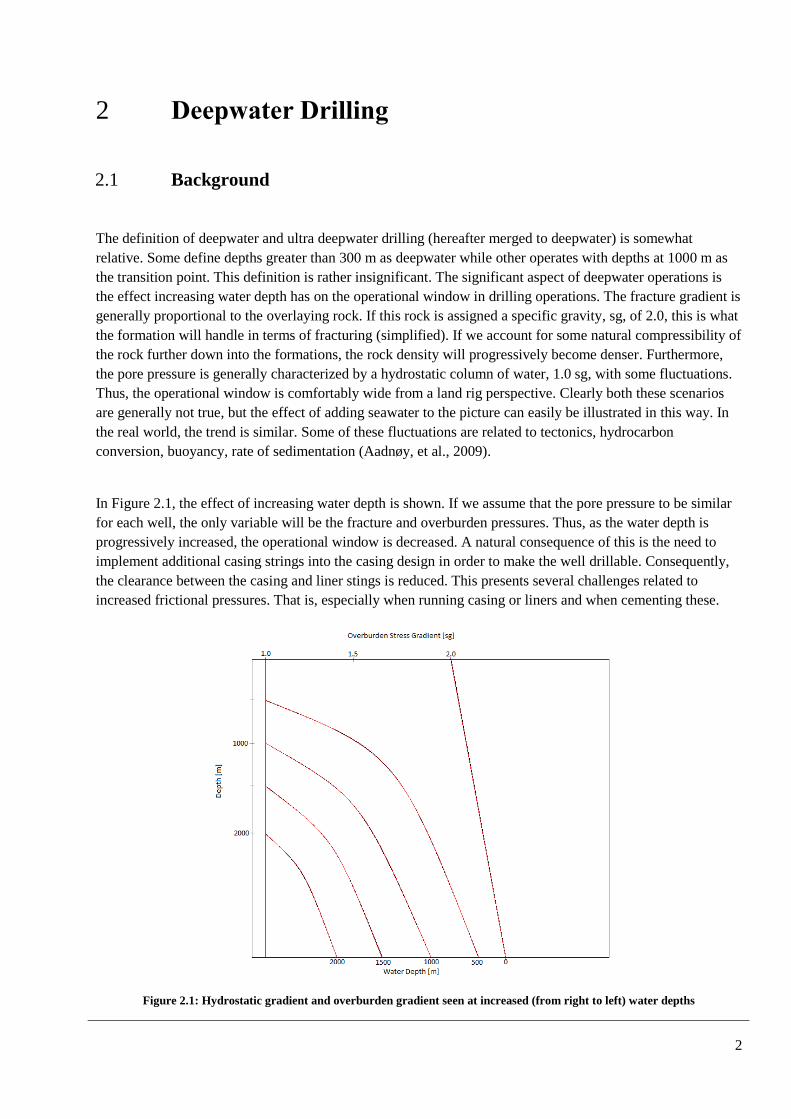
In Figure 2.1, the effect of increasing water depth is shown. If we assume that the pore pressure to be similar

for each well, the only variable will be the fracture and overburden pressures. Thus, as the water depth is

progressively increased, the operational window is decreased. A natural consequence of this is the need to

implement additional casing strings into the casing design in order to make the well drillable. Consequently,

the clearance between the casing and liner stings is reduced. This presents several challenges related to

increased frictional pressures. That is, especially when running casing or liners and when cementing these.

Figure 2.1: Hydrostatic gradient and overburden gradient seen at increased (from right to left) water depths

3

Several other challenging effects follow as a natural consequence of the increasing water depth. These will

not be given significant focus in this thesis, but are important to mention (Aadnøy, et al., 2009):

Shallow gas/water flows

o Over-pressured

formations with high flow

potential compromising

well integrity

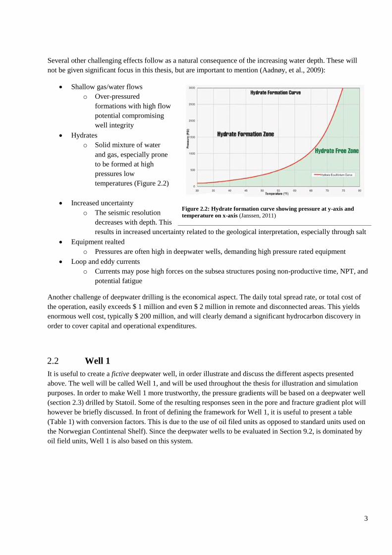
Hydrates

o Solid mixture of water

and gas, especially prone

to be formed at high

pressures low

temperatures (Figure 2.2)

Increased uncertainty

o The seismic resolution

decreases with depth. This

results in increased uncertainty related to the geological interpretation, especially through salt

Equipment realted

o Pressures are often high in deepwater wells, demanding high pressure rated equipment

Loop and eddy currents

o Currents may pose high forces on the subsea structures posing non-productive time, NPT, and

potential fatigue

Another challenge of deepwater drilling is the economical aspect. The daily total spread rate, or total cost of

the operation, easily exceeds $ 1 million and even $ 2 million in remote and disconnected areas. This yields

enormous well cost, typically $ 200 million, and will clearly demand a significant hydrocarbon discovery in

order to cover capital and operational expenditures.

Well 1 2.2

It is useful to create a fictive deepwater well, in order illustrate and discuss the different aspects presented

above. The well will be called Well 1, and will be used throughout the thesis for illustration and simulation

purposes. In order to make Well 1 more trustworthy, the pressure gradients will be based on a deepwater well

(section 2.3) drilled by Statoil. Some of the resulting responses seen in the pore and fracture gradient plot will

however be briefly discussed. In front of defining the framework for Well 1, it is useful to present a table

(Table 1) with conversion factors. This is due to the use of oil filed units as opposed to standard units used on

the Norwegian Contintenal Shelf). Since the deepwater wells to be evaluated in Section 9.2, is dominated by

oil field units, Well 1 is also based on this system.

Figure 2.2: Hydrate formation curve showing pressure at y-axis and

temperature on x-axis (Janssen, 2011)

4

From Multiply With Factor of To

kg 2.20 lb

m 3.28 ft

sg 8.35 ppg

bar 14.50 psi

Table 1: Conversion table of frequently used units

We may start by assigning a water depth of 2 438.4 m TVD to Well 1. The water depth is chosen for practical

reasons, whereas 2 438.4 m corresponds to 8 000 ft. Here, a semi-submersible is to drill an exploration well

28 000 ft TVD. The first 8 000 ft consequently has a gradient of approximately 1.0 specific gravity, sg,

(seawater). At 8 000 ft TVD, the formation rock gradient is introduced and the overburden gradient at a

specific depth is a combination of 1.0 sg and ~2.0 sg. As the well is drilled deeper the overburden will

converge towards the overburden gradient seen from a land well perspective (Figure 2.1).

Pore pressure can also be slightly adjusted or increased in this top section, which can be related to fine

grained sediments. Major basins being developed today sedimentation in deepwater environments is

dominated by fine grained sediments. The effect of low permeability and rapid burial rate may create an over

pressured zone, also referred to as under-compaction. The low permeability environment formed effectively

block communication throughout the sedimentary layers. As the sedimentation and burial continue, sediments

are hindered from compaction due to the trapped incompressible fluid. Thus, an over pressured environment

is formed (Aadnøy, et al., 2009).

We may also include a salt zone from 14 000 ft to 18 000 ft. Many sedimentary basins have sequences of

evaporates. This is often seen in closed sedimentary basins where evaporation exceeds inflow, i.e. less water

inn than what is lost by evaporation. Thick accumulations of salt settle in the basin, successively buried by

new sediments. The special feature of salt is that it behaves like a fluid. When salt is subjected to differential

stresses it will over time flow. The effect of overlying sediment deposition and tectonics will clearly influence

the behavior of salt. Salt is at the same time incompressible as opposed to sedimentary rock. This will cause

the salt to move upward if it is able to. Hence, the fracture gradient is affected by these tectonic movements

and salt fluctuations. This is often a contributor to the challenges seen when drilling through and exiting the

salt zone. Firstly, there are uncertainties related to the actual depth of base of salt, BOS, due to the poor

seismic visibility through salt. Secondly, salt migration often creates a so called rubble zone. The zone is

dominated by faults, fractured rock and pressure variations. This often makes the salt exit particularly

challenging (R.R Israel, et al., 2008).

By adding source rock at 30 000 ft and a cap rock or seal at approximately 25 000 ft, an abnormal pressure

zone can be formed. Through compaction and thermal effect as the sediments are buried, the source rock may

form hydrocarbons. Since the sediments often are buried in a marine environment, water is naturally present.

As hydrocarbons escape the source rock, it will tend to move upwards due to buoyancy. If we assume contact

from surface down to water below the cap rock, a normal pore pressure will be seen and the pressure

becomes:

1

5

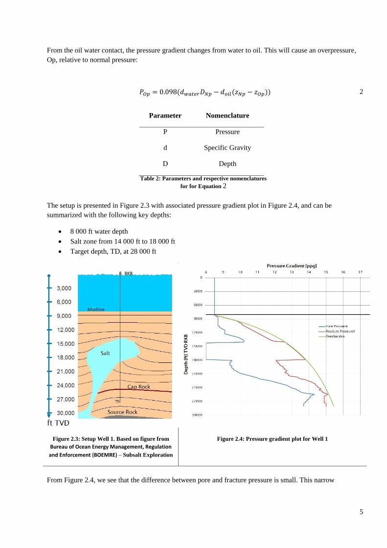
From the oil water contact, the pressure gradient changes from water to oil. This will cause an overpressure,

Op, relative to normal pressure:

2

The setup is presented in Figure 2.3 with associated pressure gradient plot in Figure 2.4, and can be

summarized with the following key depths:

8 000 ft water depth

Salt zone from 14 000 ft to 18 000 ft

Target depth, TD, at 28 000 ft

Figure 2.3: Setup Well 1. Based on figure from

Bureau of Ocean Energy Management, Regulation

and Enforcement (BOEMRE) – Subsalt Exploration

Figure 2.4: Pressure gradient plot for Well 1

From Figure 2.4, we see that the difference between pore and fracture pressure is small. This narrow

Parameter Nomenclature

P Pressure

d Specific Gravity

D Depth

Table 2: Parameters and respective nomenclatures

for for Equation 2

6

operating window is generally seen in deepwater wells (Figure 2.1), and is a typical deepwater effect. The

fracture gradient in Figure 2.4 is based on an overburden gradient of 2.2 sg of the form:

3

In Equation 3, parameter a and b are simply constants for expressing water and rock depth, D, is increased.

The plot can be summed up with these bulletins:

Pore pressure gradient

o Rapid burial rate with fine sediments cause some increase in the shallow sections

o Salt zone is dominated by hydrostatic gradient

o Subsalt is over-pressured and dominated by relatively high pressures

Fracture gradient

o Generally follows the overburden gradient, Equation 6

o Below BOS the fracture gradient is reduced (Rubble zone)

Validity of Well 1 2.3

The scope of Well 1 is not to create a detailed drilling program for drilling the well. The scope is rather to

create a simple trustworthy well design that can be used for further analysis and simulations. This will be

explained further in Section 9. In order to verify the validity of Well 1, the deepwater well from the GoM, in

which Well 1 is based on, will be briefly presented. In Figure 2.5, the vertical seismic profile of the well is

shown.

Figure 2.5: Well A, GoM (Statoil, 2012)

7

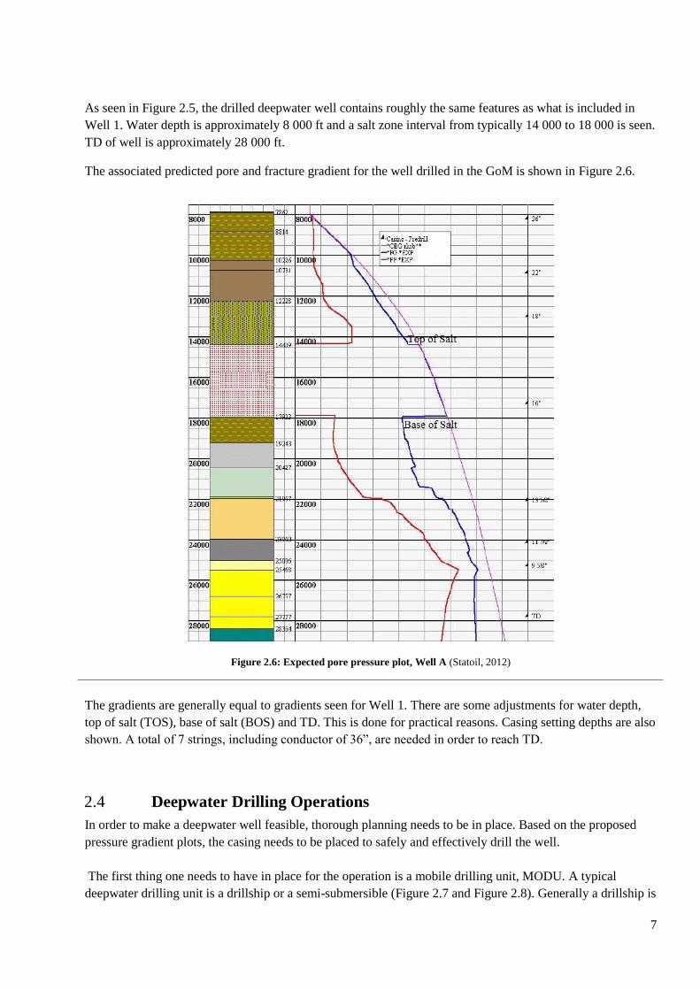
As seen in Figure 2.5, the drilled deepwater well contains roughly the same features as what is included in

Well 1. Water depth is approximately 8 000 ft and a salt zone interval from typically 14 000 to 18 000 is seen.

TD of well is approximately 28 000 ft.

The associated predicted pore and fracture gradient for the well drilled in the GoM is shown in Figure 2.6.

The gradients are generally equal to gradients seen for Well 1. There are some adjustments for water depth,

top of salt (TOS), base of salt (BOS) and TD. This is done for practical reasons. Casing setting depths are also

shown. A total of 7 strings, including conductor of 36”, are needed in order to reach TD.

Deepwater Drilling Operations 2.4

In order to make a deepwater well feasible, thorough planning needs to be in place. Based on the proposed

pressure gradient plots, the casing needs to be placed to safely and effectively drill the well.

The first thing one needs to have in place for the operation is a mobile drilling unit, MODU. A typical

deepwater drilling unit is a drillship or a semi-submersible (Figure 2.7 and Figure 2.8). Generally a drillship is

Figure 2.6: Expected pore pressure plot, Well A (Statoil, 2012)

8

more suited for deepwater operations. This is mainly due to the excessive payloads and its mobility. The

semi-submersible is superior to drillships when it comes to motion handling. Both of the drilling vessels

shown below are equipped with dual derricks. This is very useful in order to effectively drill the well. Here,

one derrick may be drilling while the other derrick is preparing for running casing. This is especially related

to the tophole sections. After the section is drilled, the bit is tipped out of hole. The rig is then skidded,

positioning the casing over well center. At this point, the casing is already run down to seabed and is ready to

be run directly into the well after moving or skidding the rig to well center.

Figure 2.7: Discoverer Americas ©Transocean

Figure 2.8: Maersk Developer © Maersk Drilling

The casing design is often influenced by the increased water depths. By comparing pressure plots form a

conventional offshore well with Well 1, Figure 2.9 and Figure 2.10, the narrow operating window is clearly

illustrated. The consequence of this is normally additional casing stings in order to reach TD. This means that

both the conventional casing setup needs to accommodate one or several casing strings in addition to a

conventional 30” - 20” - 13 3/8” - 9 5/8” setup. Usually, the surface casing is modified, typically to a 22”

surface casing. In this way, larger intermediate casings can be run in order to make extra casings or liners

feasible. This is especially related to the small clearance seen between the casing strings. A widely used

option is to incorporate two liners between the 22” surface casing and 13 5/8” casing. Here, 18” and 16” liners

are hung off in the 22” surface casing after drilling the respective sections. After drilling and cementing the 13

5/8” section, some well designs needs to incorporate a 11 7/8” liner in order to reach TD. That is, after setting

the 11 7/8” liner, a subsequent 9 5/8” liner is set to enable drilling into the potential reservoir. As one can

imagine, additional casing strings gives less clearance between the casings, although the surface casing is

increased by two inches. For example, the clearance between a 13 5/8” (88.2 lb/ft) casing and a 11 7/8” (71.8

lb/ft) liner, yields a clearance of 0.14”.

9

Figure 2.9: Pressure gradient plot from the Statfjord

field. Note that units are in [m] and [sg]

Figure 2.10: Mud program with casing setting depths for well 1 in

order to reach target depth. Note that units are in [ft] and [ppg]

In Figure 2.9 the casing setting depths and mud weights are illustrated for a typical offshore well in water

depths of approximately 150 m. In Figure 2.10 the same data is shown for Well 1. The depths are based on the

setting depths of Well A. Some brief and important considerations will be listed:

Secure deep enough surface casing depth

Set 16” liner before exiting salt section (Rubble zone)

Safety margins with respect to pore and fracture pressure (Section 7)

Well 1 is clearly more sensitive to pressure fluctuations with regards to the operating window, especially after

exiting the salt section (Figure 2.10). Furthermore, if the casing is 4 000 – 5 000 m long (e.g. 13 5/8” casing

in Well 1), enormous surge pressures will be created while running and cementing the casing. The aspect of

surge pressure will be discussed in more detail in Section 3. As a product of this, special equipment is used in

order to reduce the surge pressures created. This will be discussed in section 6.5. After the casing is in place,

the section is cemented. Again, special care needs to be taken in order to maintain well integrity.

The tophole sections are drilled without riser, analogous to a conventional offshore well. As seen in Figure

2.10, the pore pressure seems to increase slightly from seabed and down to top of salt. At these shallow

sections of the well, challenges related to shallow water flows and gas may also alter the predicted pressure

gradient profile of the well. Thus, it may be necessary to utilize a weighted mud system prior to installing the

riser. This can be done either by using weighted mud and pump this up the annulus and directly to seafloor

(pump and dump). This is the conventional way of dealing with this challenge. Another option is to use a

return to rig system. One (if only) technology that allows for this without using pump and dump strategy is

the Riserless Mud Recovery, RMR™. This technology enables mud return to rig by use of a suction module

and subsea pump. Here the mud level is monitored in the suction module and adjusted by the subsea pump.

After cementing the 20” (or 22”) casing, the riser-Lower marine Riser Package, LMRP-BOP is run and

connected to the wellhead. Thus, the rig has a closed loop for the mud system through the riser system.

10

Figure 2.11: RMR™ system from AGR Drilling Services (Newswise,

2009)

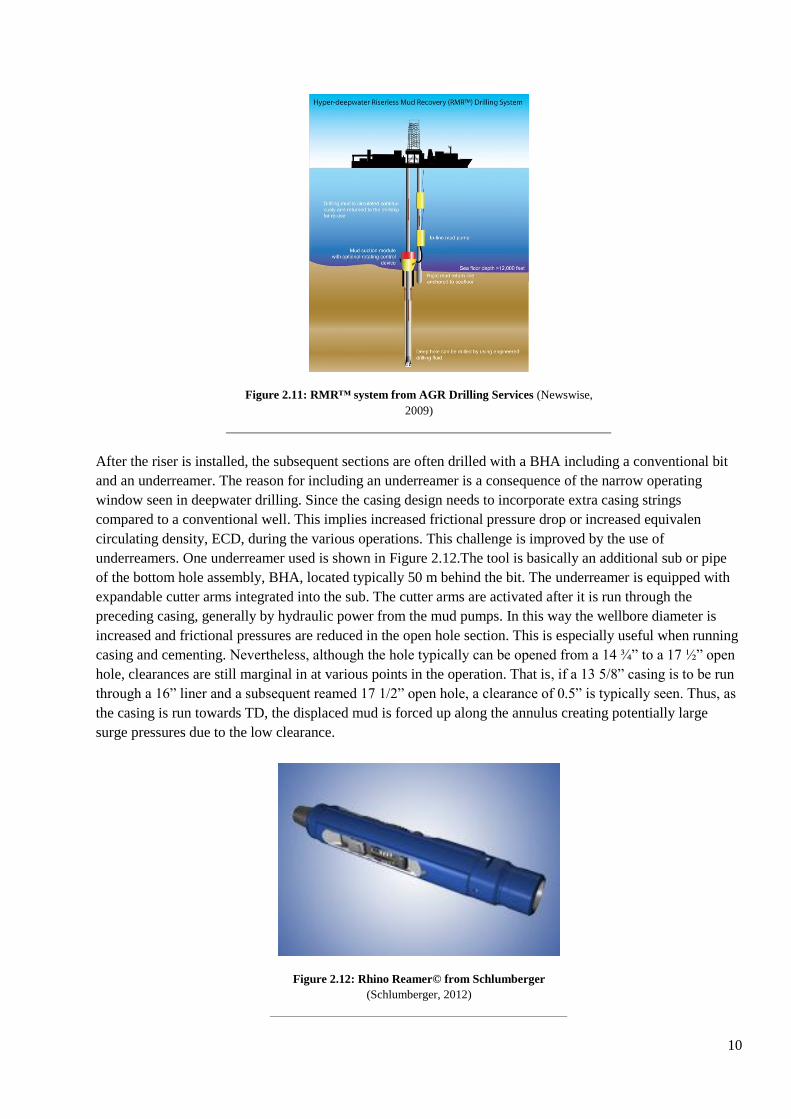
After the riser is installed, the subsequent sections are often drilled with a BHA including a conventional bit

and an underreamer. The reason for including an underreamer is a consequence of the narrow operating

window seen in deepwater drilling. Since the casing design needs to incorporate extra casing strings

compared to a conventional well. This implies increased frictional pressure drop or increased equivalen

circulating density, ECD, during the various operations. This challenge is improved by the use of

underreamers. One underreamer used is shown in Figure 2.12.The tool is basically an additional sub or pipe

of the bottom hole assembly, BHA, located typically 50 m behind the bit. The underreamer is equipped with

expandable cutter arms integrated into the sub. The cutter arms are activated after it is run through the

preceding casing, generally by hydraulic power from the mud pumps. In this way the wellbore diameter is

increased and frictional pressures are reduced in the open hole section. This is especially useful when running

casing and cementing. Nevertheless, although the hole typically can be opened from a 14 ¾” to a 17 ½” open

hole, clearances are still marginal in at various points in the operation. That is, if a 13 5/8” casing is to be run

through a 16” liner and a subsequent reamed 17 1/2” open hole, a clearance of 0.5” is typically seen. Thus, as

the casing is run towards TD, the displaced mud is forced up along the annulus creating potentially large

surge pressures due to the low clearance.

Figure 2.12: Rhino Reamer© from Schlumberger

(Schlumberger, 2012)

11

After the hole is drilled and reamed, casing is to be run and cemented. Tripping into the hole is done

conventionally, but one often has more restrictions with regards to tripping speed of the pipe. This is mainly

related to surge pressures created when tripping in/out of the hole. Equipment related restrictions are usually

also present. This is related to drawwork capability, acceleration and deceleration of sting, wellbore

inclination, running past well head and other equipment and further on. Maximum tripping speeds are relative

from rig to rig, but tripping 3 000 ft/hr or 50 ft min of drill pipe is considered as fast. The tripping speed of

one stand is typically of parabolic character. As the slips are removed, the pipe is allowed to accelerate into

the hole, and the pipe running speed is increase. As the top drive moves toward rig floor, the pipe speed is

decelerated by the drawwork brakes in order set the slips and make up a new pipe. Thus, the speed of 50

ft/min mentioned above is the average speed spent on one stand including making up the connection. The

maximum speed of the pipe is typically 1 m/s or approximately 190 ft/min, this is due to limitations of the

drawworks (SSC, 2012).

Figure 2.13 gives a good illustration on the actual situation when comparing a conventional offshore well

with a deepwater well. Not only is Well 1 three times deeper than a Statfjord well, but it is also incorporates

three extra casing/liner strings. This means that tripping in and out of hole becomes a significant factor of the

drilling operation, and needs to be especially tuned in order to minimize time spent on tripping.

Figure 2.13: Typical casing program for a well at the Statfjord field versus Well 1

After the casing or liner has been run to TD, cementing is required in order to obtain zonal isolation and

structural support (Section 7). The typical feature of a deepwater cement job is lightweight cement. This is

also related to the operational window, and the fact that conventional cement has a relative high density.

Thus, the cement density needs to be sufficiently lowered without compromising the cement strength

requirements. In the tophole sections were cementing to surface often is required, a foamed cement may be

needed in order not to fracture the formations. As for the intermediate and production casings one often uses a

lightweight lead cement type and heavier tail cement over the casing shoe in order to mitigate formation

damage and fracturing. This will be further discussed in Section 6. The important factor is to evaluate these

challenges and initiate mitigating actions if they are needed.

12

Well Integrity 3

The immediate factor securing well integrity while drilling and cementing is the fluid column in the well.

When we enter the deepwater drilling regime the operational window is affected, as discussed in the previous

chapter. In order to maintain well integrity the equivalent static density, ESD, and ECD needs to be balanced

between pore- and fracture pressure throughout the operation. If the pore pressure exceeds the pressure in the

well, a gain or kick may be induced. Influx cease when the pressure is equalized, typically by the kick itself or

by closing the BOP.

Another important puzzle of wellbore integrity is rock mechanics. It is well know that borehole stability falls

into two main categories:

Borehole fracturing at high borehole pressures

Borehole collapse at low borehole pressures.

Before we describe these rock failures further it is useful to review the stress components acting on the

borehole wall (Aadnøy, 2010).

Firstly, we have overburden load created from the successively deposited sediments. This is often referred to

as the vertical stress component. The vertical stress is seen as a constant, and is not influenced when drilling.

As new formation is drilled a new stress is introduced to the formation and borehole wall in terms of radial

stress. This is the pressure exerted by the fluid column in the borehole. The newly formed borehole will also

experience a tangential stress, acting around the circumference. This is generally referred to as hoop stress.

Hoop stress in strongly dependent on the radial stress, and the dependence can be written in its simplest form

as:

4

Parameter Nomenclature

Hoop Stress

Average Stress

Radial Stress

Borehole Pressure

Table 3: Parameters and nomenclature used in Equation 4

In Equation 4 the in-situ horizontal stresses is thought to be of isotropic nature. By this we mean that the in-

situ horizontal stresses do not change. This will approximately be the case in a relaxed depositional basin with

a so-called hydrostatic stress state. Due to this assumption, we may use an average stress ( ) for the average

horizontal in-situ stresses.

If we use figure Figure 3.1, we see that with low borehole pressure, the hoop stress is high. A natural

consequence of lowering the mud weight is borehole collapse or a kick. Clearly a kick is generally induced by

Po > Pw, but the collapse is due to the high hoop stress. This is classified as a shear failure. On the other hand,

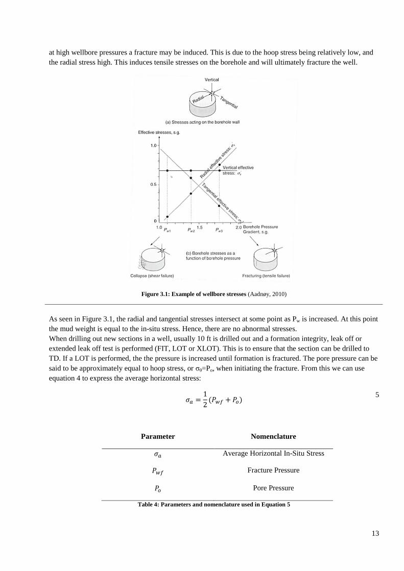
13

at high wellbore pressures a fracture may be induced. This is due to the hoop stress being relatively low, and

the radial stress high. This induces tensile stresses on the borehole and will ultimately fracture the well.

Figure 3.1: Example of wellbore stresses (Aadnøy, 2010)

As seen in Figure 3.1, the radial and tangential stresses intersect at some point as Pw is increased. At this point

the mud weight is equal to the in-situ stress. Hence, there are no abnormal stresses.

When drilling out new sections in a well, usually 10 ft is drilled out and a formation integrity, leak off or

extended leak off test is performed (FIT, LOT or XLOT). This is to ensure that the section can be drilled to

TD. If a LOT is performed, the the pressure is increased until formation is fractured. The pore pressure can be

said to be approximately equal to hoop stress, or σθ=Po, when initiating the fracture. From this we can use

equation 4 to express the average horizontal stress:

5

Parameter Nomenclature

Average Horizontal In-Situ Stress

Fracture Pressure

Pore Pressure

Table 4: Parameters and nomenclature used in Equation 5

14

From equation 5 we see that the average horizontal stress is equal to the average pressure between the pore

and fracture pressure. As indicated above, a situation with non-hydrostatic horizontal stresses is more

complex.

Ideally the mud weight should be equal to the average horizontal stresses in order to avoid borehole problems.

This is a challenging task when we include all operations done when drilling and cementing a well.

Firstly, as the well is drilled deeper, the frictional pressure drop is also increased. Consequently the

differential pressure between ECD and ESD increases. This makes it challenging to maintain a stable

borehole pressure. That is, these differences between ECD and ESD are typically experienced as shock waves

travelling through the fluid. Since circulation in the well cyclically is switched on an off, typical borehole

fatigue failure may occur. Clearly, this effect is amplified as the well is drilled deeper.

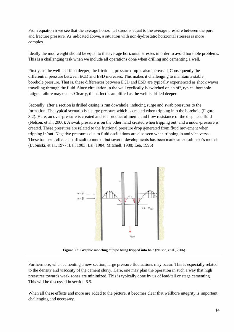
Secondly, after a section is drilled casing is run downhole, inducing surge and swab pressures to the

formation. The typical scenario is a surge pressure which is created when tripping into the borehole (Figure

3.2). Here, an over-pressure is created and is a product of inertia and flow resistance of the displaced fluid

(Nelson, et al., 2006). A swab pressure is on the other hand created when tripping out, and a under-pressure is

created. These pressures are related to the frictional pressure drop generated from fluid movement when

tripping in/out. Negative pressures due to fluid oscillations are also seen when tripping in and vice versa.

These transient effects is difficult to model, but several developments has been made since Lubinski’s model

(Lubinski, et al., 1977; Lal, 1983; Lal, 1984; Mitchell, 1988; Lea, 1996)

Figure 3.2: Graphic modeling of pipe being tripped into hole (Nelson, et al., 2006)

Furthermore, when cementing a new section, large pressure fluctuations may occur. This is especially related

to the density and viscosity of the cement slurry. Here, one may plan the operation in such a way that high

pressures towards weak zones are minimized. This is typically done by us of lead/tail or stage cementing.

This will be discussed in section 6.5.

When all these effects and more are added to the picture, it becomes clear that wellbore integrity is important,

challenging and necessary.

15

Normalization of data 4

When analyzing data and narrow operating windows, normalization of the data may be significant for the

analysis. Often the geologists uses mean sea level, MSL, as depth reference while the driller operates with the

drill floor or rotary kelly bushing, RKB. This typically gives a vertical difference of 30 m with respect to

reference point. Furthermore, if the analysis includes semi-submersibles and concrete platforms, the reference

point will also be inconsistent. In order to account for this effect, one usually performs data normalization.

This basically means that all data points are normalized to a common reference depth, typically MSL or RKB.

If we build further on the example in Well 1, one scenario could be a semi-submersible drilling rig versus a

drill ship. Here the difference in elevation could be significant.

Figure 4.1: Semi-submersible versus drillship. Figure based on figure from Wikipedia (Wikipedia, 2012)

If we were to correlate to MSL, we need to know the height from RKB to MSL from each vessel, hf. We also

would need to know the pressure gradient in each case. The pressure gradient is directly proportional to the

specific gravity of mud,

. Relative to drill floor, the pressure at any given depth, D, becomes:

6

When expressing this with reference depth to MSL we know that the pressure at any point is equal. The

difference is related to the pressure gradient:

7

By equating these to equations, we get an expression for the correct pressure gradient:

16

8

By using the individual hf for the semi-submersible and drillship, we are able to normalize the data between

the two. The deduction when normalizing from one RKB to another is identical to the RKB to MSL

normalization presented above.

9

When normalizing to RKB at the drill ship, the equation then becomes:

10

Parameter Nomenclature

hf Height RKB-MSL

d Specific gravity

P Pressure

D Depth from RKB

RKB elevation difference

Table 5: Parameters and nomenclature

17

Drilling Fluids 5

Rheology 5.1

The flow of fluids is a highly complex science, and is somewhat examined through rheology. Rheology is

defined as the study of the deformation and flow of materials. The key in this study is the viscosity of fluids,

which basically is the measure of resistance to an applied stress on the fluid. The viscosity is necessary in

order to describe the flow rate (shear rate) and the pressure gradient (shear stress). These are fundamental

elements of drilling and cement fluids, which are carefully evaluated and designed in order to secure a solid

drilling and cement section. On the rig, the circulation fluid is measured on a daily basis and, this especially

important for narrow operating windows. When measuring the rheology of a fluid a coaxial cylindrical

viscometer is generally used. The fluid is contained in a large cup and the actual measurements are performed

by use of a rotor and a bob (stator). The rotor rotates at various preset rates. The bob is fixed to a torsional

spring, and deflect from its initial position depending on the torsion created by the rheology of fluid. In this

way shear rate (s-1

) and shear stress (lbf/ft2) are measured. Other important measurements performed with the

viscometer are yield and gel strength. These are measurements of the attractive forces that exist between the

particles in the fluid. Here the yield is measured under flowing conditions, while gel strength under ten

seconds static period followed by 3 revolutions per minute, rpm. The maximum deflection is defined as the

gel strength.

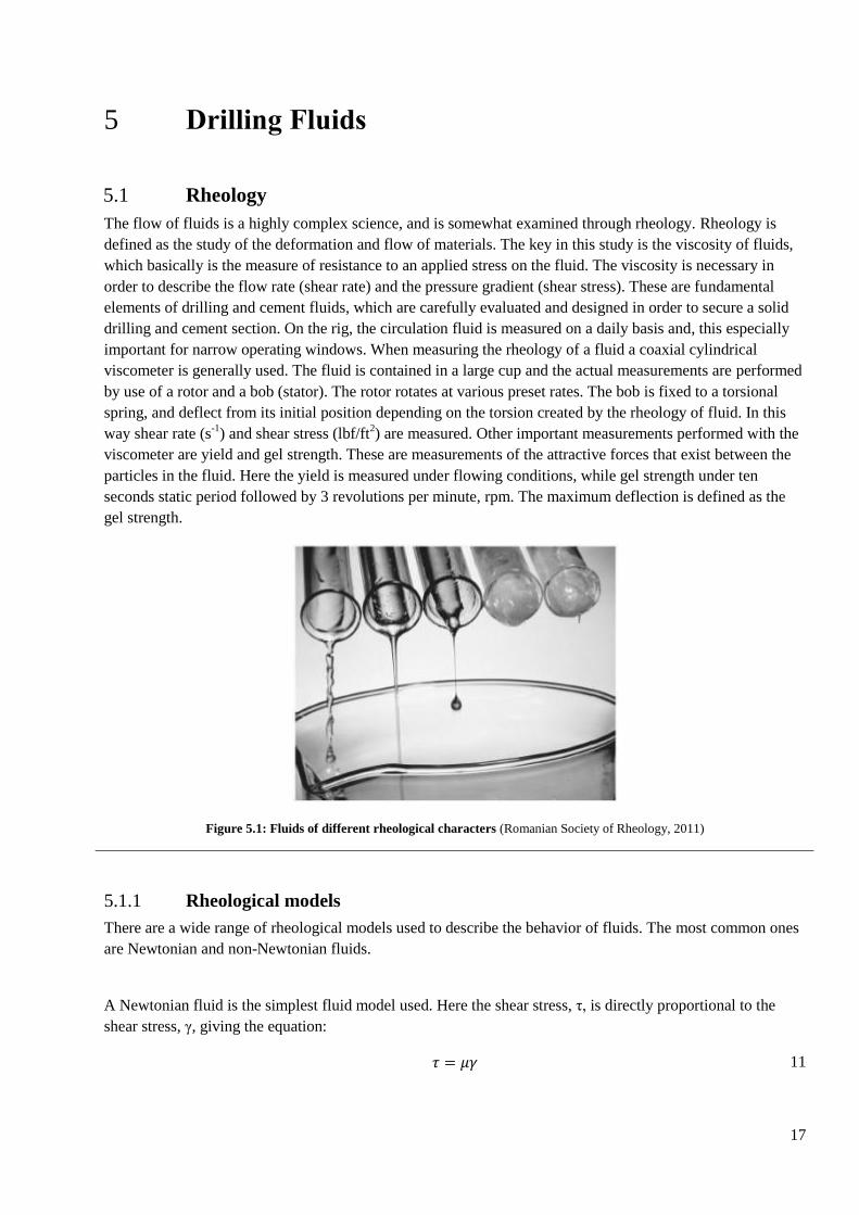
Figure 5.1: Fluids of different rheological characters (Romanian Society of Rheology, 2011)

Rheological models 5.1.1

There are a wide range of rheological models used to describe the behavior of fluids. The most common ones

are Newtonian and non-Newtonian fluids.

A Newtonian fluid is the simplest fluid model used. Here the shear stress, τ, is directly proportional to the

shear stress, γ, giving the equation:

11

18

The fluid behavior is illustrated in Figure 5.2. As Equation 11 shows, the viscosity, μ, of the fluid represents

the slope of the curve. The viscosity is not dependent on flow conditions, but rather on pressure and

temperature. Common Newtonian fluids are water, gasoline and light oil.

Non-Newtonian fluids are recognized by being a fluid which differs from the Newtonian fluid behavior. This

means that the fluid has a different shear-stress/shear-rate relationship compared to a Newtonian fluid. The

main difference basically lies in the dependency viscosity have on shear rate. As stated above, a Newtonian

fluid has constant viscosity with varying shear rate. For a non-Newtonian fluid the viscosity can either

increase with shear rate (shear thickening) or decrease with shear rate (shear thinning). Most drilling muds,

cements slurries and heavy oils are shear thinning. Common non-Newtonian models include Power-law,

Bingham plastic and Herschel-Bulkley fluids.

Power-law fluids are recognized by responding immediately after applying a pressure differential, analogous

to a Newtonian fluid. The relationship between shear stress and shear rate is no longer linear, which is

illustrated in Figure 5.2. The fluid behavior is described by the following equation:

12

Depending on the value of n, <1 or >1, the fluids are classified as shear thinning or shear thickening

respectively. As long as a Power-law fluid is within the laminar flow regime, the fluid will follow shear-

stress/shear-rate relationship. When entering the turbulent flow regime, the fluid’s frictional pressure drop

increases at a higher rate compared to the Power-law model. A typical shear thinning fluid is hair gel while

sand soaked in water can be classified as shear thickening.

A Bingham Plastic fluid is in some sense similar to a Newtonian fluid. The main difference lies in the

initiation point of flow. As for a Newtonian fluid, it flows at any finite shear stress. Whereas a Bingham

Plastic fluid requires a certain amount of shear stress in order to initiate flow. This is seen in Figure 5.2. This

threshold is referred to as the yield stress, τy. The fluid behavior is described by:

13

If the fluid is flowing in laminar conditions it starts up by showing non-linear characteristics, and as the shear

rate/shear stress is increased the behavior is more of a linear characteristic. An example of a Bingham Plastic

fluid is drilling mud.

The last model presented is the Herschel-Bulkley fluid model. This is basically a combination of Power law

and Bingham plastic behaviors. There is a certain threshold or pressure differential which needs to be in place

in order to initiate flow. When the fluid has started flowing, the behavior follows the pattern of a Power law

fluid. The fluid behavior is described by:

14

As long as the flow is laminar, the behavior of the fluid is described by this equation. When the flow regime

enters the turbulent flow regime, the frictional pressure drop is increased faster than predicted by the model.

An example of a fluid that fits Herschel-Bulkley model is cement.

19

Figure 5.2: Different Newtonian and non-Newtonian rheological models (Nelson, et al., 2006)

Water Based Mud 5.2

Drilling a well include the selection of which type of drilling fluid or mud one should use. This selection is

based on pressure and temperature regime, formations to be drilled, environmental aspect, economical aspect

and so on. A balanced function of viscosity, lubricants, weighting agents, lost circulation materials and so

forth, in order to effectively reach TD is generally the main objective.

The simplest form of drilling fluid is water based fluid of non-inhibitive form. This is typically the drilling

fluid used in spud drilling (seawater), bentonite-treated mud and lignite mud. It is inexpensive, easy to make

and maintain. The limitations are related to reactive shales, high temperature wells and formations containing

certain contaminants, e.g. H2S (Azar, et al., 2007).

Water based inhibitive muds are generally used to withstand the challenges related to reactive shales. The

purpose is to restrain hydration, swelling and disintegration of shale or other substances. Calcium based muds,

salt based muds, potassium based muds and polymer drilling muds are some of the inhibitive muds available

(Azar, et al., 2007; Schlumberger, 2012).

Oil Based Mud 5.3

A drilling fluid is classified as oil based if the continuous liquid (external phase) is oil, typically mineral oil.

There are two types of oil based mud, OBM; oil or invert emulsion muds. Oil muds are characterized by the

content of dispersed water being less than 5 %. An invert emulsion mud on the other hand has dispersed water

content greater than 5 %. In either case, the continuous phase in the fluid is oil and the dispersed (internal) is

water. Advantages with an OBM are their ability to effectively withstand contamination from H2S, CO2, salt,

anhydrite and active shales (Azar, et al., 2007). Lubricating effect, temperature stability and few additives

needed are also good examples of why OBMs are widely used. The main drawback of OBMs is related to the

environmental impact of the fluid. Due to the content of materials which may be harmful to the environment,

waste management is essential. Another important aspect when using OBMs are the solubility of gas in the oil

phase of the mud. Consequently, gas may dissolve into the oil phase during drilling under the “right” pressure

and temperature conditions. As the mud is circulated up the wellbore, the fluid enters the two phase envelope

20

and boils out of the liquid phase, inducing a kick. In other words, the oil based mud may hide a kick and

suddenly release it further up the wellbore. This is especially critical if it were to occur after passing the blow

out preventer, BOP, in deep water wells.

Synthetic Based Mud 5.4

Synthetic based muds, SBM, are very much like oil based drilling fluids. The external phase is now replaced

by a synthetic phase, i.e. an oil phase is replaced by an artificial (synthetic) phase. The synthetic phase is

typically organic chemicals, principally containing carbon, hydrogen and oxygen. In general SBMs exhibit

much of the desirable properties of OBMs, but are also more environmental friendly. This is due to the

removal of polynuclear aromatic hydrocarbons, faster biodegradability, lower bioaccumulation and in some

cases less drilling waste volume. Consequently, SBMs are more expensive compared to OBMs. (Orszulik,

2008). All of the three major service vendors in the oil industry, Baker Hughes, Halliburton and

Schlumberger, provide SBMs and are especially linked to deep water operations. The reasons for this are

environmental considerations and operational considerations. The operational aspect is related to the

rheological properties of SBMs. All three RHEO-LOGIC™ (Baker Hughes), ENCORE® (Halliburton) and

RHELIANT (Schlumberger) SBMs are claimed to hold flat rheology over wide temperature ranges. Since

deepwater drilling temperature profiles vary quite drastically from surface – seabed – TD (Section 7), this

fluid yields a more predictable behavior of the fluid dynamics throughout the well.

Drilling Fluid Fundamentals 5.5

The two upcoming chapters, 5.5.1and 5.5.2 , are most likely well know. It is however useful to briefly review

the fundamental function of drilling fluids and its circulation system.

Drilling Fluid Functions 5.5.1

In addition to wellbore stability that has already been mentioned in Section 3, some of the functions are:

Suspend and remove cuttings

Seal permeable formations

Cool and lubricate the bit

Provide hydraulic energy (e.g. underreamer)

21

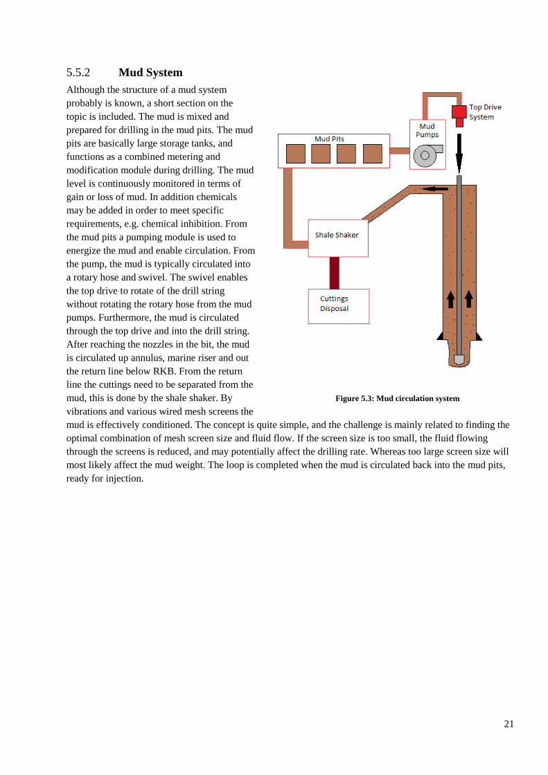
Mud System 5.5.2

Although the structure of a mud system

probably is known, a short section on the

topic is included. The mud is mixed and

prepared for drilling in the mud pits. The mud

pits are basically large storage tanks, and

functions as a combined metering and

modification module during drilling. The mud

level is continuously monitored in terms of

gain or loss of mud. In addition chemicals

may be added in order to meet specific

requirements, e.g. chemical inhibition. From

the mud pits a pumping module is used to

energize the mud and enable circulation. From

the pump, the mud is typically circulated into

a rotary hose and swivel. The swivel enables

the top drive to rotate of the drill string

without rotating the rotary hose from the mud

pumps. Furthermore, the mud is circulated

through the top drive and into the drill string.

After reaching the nozzles in the bit, the mud

is circulated up annulus, marine riser and out

the return line below RKB. From the return

line the cuttings need to be separated from the

mud, this is done by the shale shaker. By

vibrations and various wired mesh screens the

mud is effectively conditioned. The concept is quite simple, and the challenge is mainly related to finding the

optimal combination of mesh screen size and fluid flow. If the screen size is too small, the fluid flowing

through the screens is reduced, and may potentially affect the drilling rate. Whereas too large screen size will

most likely affect the mud weight. The loop is completed when the mud is circulated back into the mud pits,

ready for injection.

Figure 5.3: Mud circulation system

22

Cementing 6

In this chapter, the basic components of cement slurry will firstly be described. The subsequent section will

the present various casing tools typically used in the cement job. After an introduction to the components and

tools used, various aspects (pre – during – post) of a cement job will be evaluated. A natural place to start is to

discuss the use and functions of washers and spacers.

Washers and Spacers 6.1

The objective of a washer or prewash is to dilute and wash away gelled

mud. The fluid is generally characterized by an unweighted Newtonian

fluid. This is to allow high flow rates and consequently a turbulent flow

regime. The volume being pumped should be maximized at these

conditions, although the operating window is the governing factor.

The spacer is used to secure sufficient mud removal, and needs to be

compatible with both the mud and cement. The density and rheology of the

spacer is carefully designed. The design can typically include viscosifiers,

dispersants, surfactants, fluid loss control agents and weighting agents.

Viscosifiers are necessary in order to suspend the weighting agents and

control the rheological properties. This can generally be done by adding

water soluble polymers and clays. In order to achieve good mud removal,

viscosity of the spacer is generally kept high and fluid flows within the

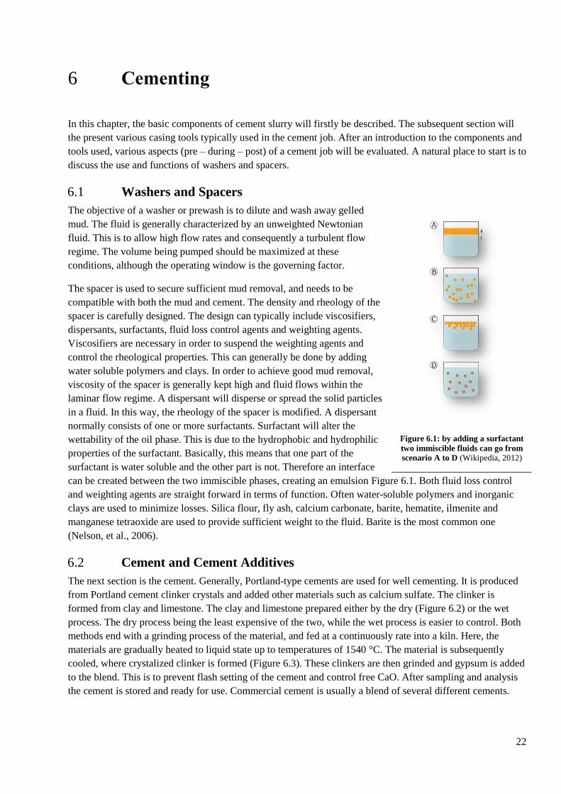
laminar flow regime. A dispersant will disperse or spread the solid particles

in a fluid. In this way, the rheology of the spacer is modified. A dispersant

normally consists of one or more surfactants. Surfactant will alter the

wettability of the oil phase. This is due to the hydrophobic and hydrophilic

properties of the surfactant. Basically, this means that one part of the

surfactant is water soluble and the other part is not. Therefore an interface

can be created between the two immiscible phases, creating an emulsion Figure 6.1. Both fluid loss control

and weighting agents are straight forward in terms of function. Often water-soluble polymers and inorganic

clays are used to minimize losses. Silica flour, fly ash, calcium carbonate, barite, hematite, ilmenite and

manganese tetraoxide are used to provide sufficient weight to the fluid. Barite is the most common one

(Nelson, et al., 2006).

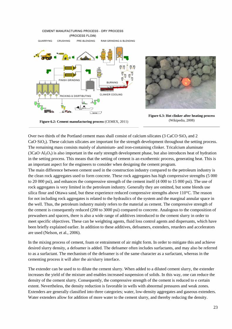
Cement and Cement Additives 6.2

The next section is the cement. Generally, Portland-type cements are used for well cementing. It is produced

from Portland cement clinker crystals and added other materials such as calcium sulfate. The clinker is

formed from clay and limestone. The clay and limestone prepared either by the dry (Figure 6.2) or the wet

process. The dry process being the least expensive of the two, while the wet process is easier to control. Both

methods end with a grinding process of the material, and fed at a continuously rate into a kiln. Here, the

materials are gradually heated to liquid state up to temperatures of 1540 °C. The material is subsequently

cooled, where crystalized clinker is formed (Figure 6.3). These clinkers are then grinded and gypsum is added

to the blend. This is to prevent flash setting of the cement and control free CaO. After sampling and analysis

the cement is stored and ready for use. Commercial cement is usually a blend of several different cements.

Figure 6.1: by adding a surfactant

two immiscible fluids can go from

scenario A to D (Wikipedia, 2012)

23

Figure 6.2: Cement manufacturing process (CEMEX, 2011)

Over two thirds of the Portland cement mass shall consist of calcium silicates (3 CaCO·SiO2 and 2

CaO·SiO2). These calcium silicates are important for the strength development throughout the setting process.

The remaining mass consists mainly of aluminium- and iron-containing clinker. Tricalcium aluminate

(3CaO·Al2O3) is also important in the early strength development phase, but also introduces heat of hydration

in the setting process. This means that the setting of cement is an exothermic process, generating heat. This is

an important aspect for the engineers to consider when designing the cement program.

The main difference between cement used in the construction industry compared to the petroleum industry is

the clean rock aggregates used to form concrete. These rock aggregates has high compressive strengths (5 000

to 20 000 psi), and enhances the compressive strength of the cement itself (4 000 to 15 000 psi). The use of

rock aggregates is very limited in the petroleum industry. Generally they are omitted, but some blends use

silica flour and Ottawa sand, but these experience reduced compressive strengths above 110°C. The reason

for not including rock aggregates is related to the hydraulics of the system and the marginal annular space in

the well. Thus, the petroleum industry mainly refers to the material as cement. The compressive strength of

the cement is consequently reduced (200 to 3000 psi) compared to concrete. Analogous to the composition of

prewashers and spacers, there is also a wide range of additives introduced to the cement slurry in order to

meet specific objectives. These can be weighting agents, fluid loss control agents and dispersants, which have

been briefly explained earlier. In addition to these additives, defoamers, extenders, retarders and accelerators

are used (Nelson, et al., 2006).

In the mixing process of cement, foam or entrainment of air might form. In order to mitigate this and achieve

desired slurry density, a defoamer is added. The defoamer often includes surfactants, and may also be referred

to as a surfactant. The mechanism of the defoamer is of the same character as a surfactant, whereas in the

cementing process it will alter the air/slurry interface.

The extender can be used to to dilute the cement slurry. When added to a diluted cement slurry, the extender

increases the yield of the mixture and enables increased suspension of solids. In this way, one can reduce the

density of the cement slurry. Consequently, the compressive strength of the cement is reduced to e certain

extent. Nevertheless, the density reduction is favorable in wells with abnormal pressures and weak zones.

Extenders are generally classified into three categories; water, low-density aggregates and gaseous extenders.

Water extenders allow for addition of more water to the cement slurry, and thereby reducing the density.

Figure 6.3: Hot clinker after heating process

(Wikipedia, 2008)

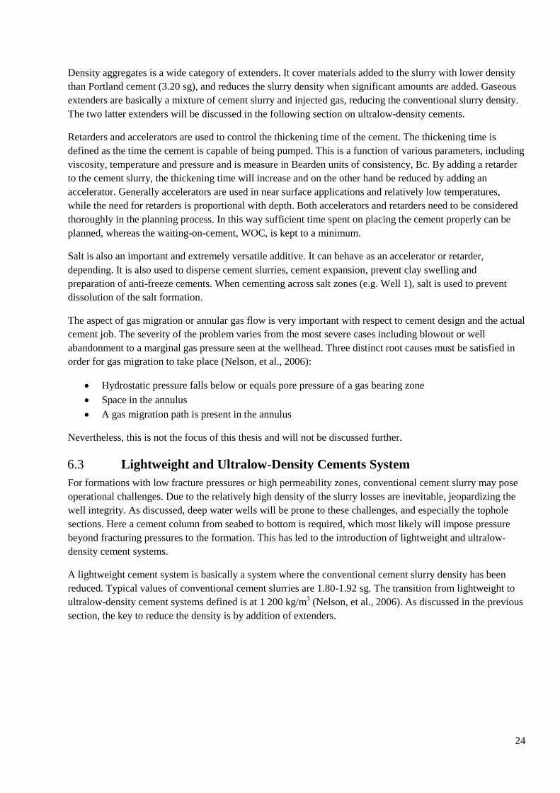
24

Density aggregates is a wide category of extenders. It cover materials added to the slurry with lower density

than Portland cement (3.20 sg), and reduces the slurry density when significant amounts are added. Gaseous

extenders are basically a mixture of cement slurry and injected gas, reducing the conventional slurry density.

The two latter extenders will be discussed in the following section on ultralow-density cements.

Retarders and accelerators are used to control the thickening time of the cement. The thickening time is

defined as the time the cement is capable of being pumped. This is a function of various parameters, including

viscosity, temperature and pressure and is measure in Bearden units of consistency, Bc. By adding a retarder

to the cement slurry, the thickening time will increase and on the other hand be reduced by adding an

accelerator. Generally accelerators are used in near surface applications and relatively low temperatures,

while the need for retarders is proportional with depth. Both accelerators and retarders need to be considered

thoroughly in the planning process. In this way sufficient time spent on placing the cement properly can be

planned, whereas the waiting-on-cement, WOC, is kept to a minimum.

Salt is also an important and extremely versatile additive. It can behave as an accelerator or retarder,

depending. It is also used to disperse cement slurries, cement expansion, prevent clay swelling and

preparation of anti-freeze cements. When cementing across salt zones (e.g. Well 1), salt is used to prevent

dissolution of the salt formation.

The aspect of gas migration or annular gas flow is very important with respect to cement design and the actual

cement job. The severity of the problem varies from the most severe cases including blowout or well

abandonment to a marginal gas pressure seen at the wellhead. Three distinct root causes must be satisfied in

order for gas migration to take place (Nelson, et al., 2006):

Hydrostatic pressure falls below or equals pore pressure of a gas bearing zone

Space in the annulus

A gas migration path is present in the annulus

Nevertheless, this is not the focus of this thesis and will not be discussed further.

Lightweight and Ultralow-Density Cements System 6.3

For formations with low fracture pressures or high permeability zones, conventional cement slurry may pose

operational challenges. Due to the relatively high density of the slurry losses are inevitable, jeopardizing the

well integrity. As discussed, deep water wells will be prone to these challenges, and especially the tophole

sections. Here a cement column from seabed to bottom is required, which most likely will impose pressure

beyond fracturing pressures to the formation. This has led to the introduction of lightweight and ultralow-

density cement systems.

A lightweight cement system is basically a system where the conventional cement slurry density has been

reduced. Typical values of conventional cement slurries are 1.80-1.92 sg. The transition from lightweight to

ultralow-density cement systems defined is at 1 200 kg/m3 (Nelson, et al., 2006). As discussed in the previous

section, the key to reduce the density is by addition of extenders.

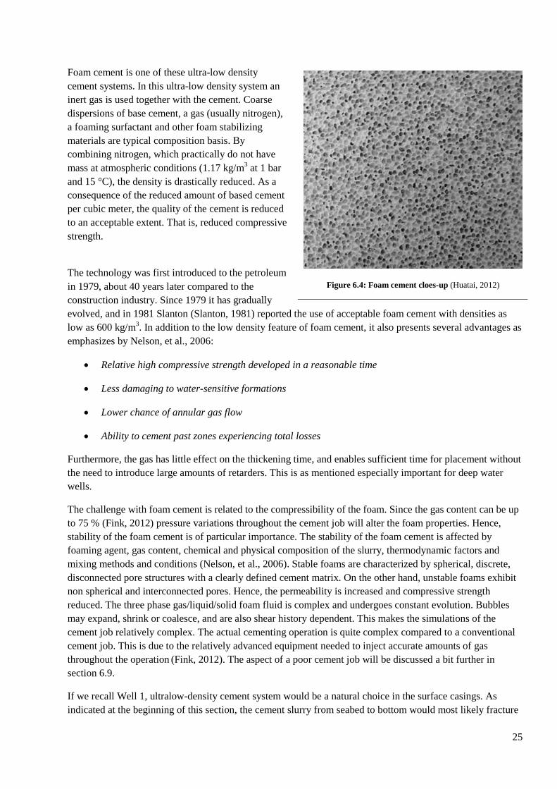
25

Foam cement is one of these ultra-low density

cement systems. In this ultra-low density system an

inert gas is used together with the cement. Coarse

dispersions of base cement, a gas (usually nitrogen),

a foaming surfactant and other foam stabilizing

materials are typical composition basis. By

combining nitrogen, which practically do not have

mass at atmospheric conditions (1.17 kg/m3 at 1 bar

and 15 °C), the density is drastically reduced. As a

consequence of the reduced amount of based cement

per cubic meter, the quality of the cement is reduced

to an acceptable extent. That is, reduced compressive

strength.

The technology was first introduced to the petroleum

in 1979, about 40 years later compared to the

construction industry. Since 1979 it has gradually

evolved, and in 1981 Slanton (Slanton, 1981) reported the use of acceptable foam cement with densities as

low as 600 kg/m3. In addition to the low density feature of foam cement, it also presents several advantages as

emphasizes by Nelson, et al., 2006:

Relative high compressive strength developed in a reasonable time

Less damaging to water-sensitive formations

Lower chance of annular gas flow

Ability to cement past zones experiencing total losses

Furthermore, the gas has little effect on the thickening time, and enables sufficient time for placement without

the need to introduce large amounts of retarders. This is as mentioned especially important for deep water

wells.

The challenge with foam cement is related to the compressibility of the foam. Since the gas content can be up

to 75 % (Fink, 2012) pressure variations throughout the cement job will alter the foam properties. Hence,

stability of the foam cement is of particular importance. The stability of the foam cement is affected by

foaming agent, gas content, chemical and physical composition of the slurry, thermodynamic factors and

mixing methods and conditions (Nelson, et al., 2006). Stable foams are characterized by spherical, discrete,

disconnected pore structures with a clearly defined cement matrix. On the other hand, unstable foams exhibit

non spherical and interconnected pores. Hence, the permeability is increased and compressive strength

reduced. The three phase gas/liquid/solid foam fluid is complex and undergoes constant evolution. Bubbles

may expand, shrink or coalesce, and are also shear history dependent. This makes the simulations of the

cement job relatively complex. The actual cementing operation is quite complex compared to a conventional

cement job. This is due to the relatively advanced equipment needed to inject accurate amounts of gas

throughout the operation (Fink, 2012). The aspect of a poor cement job will be discussed a bit further in

section 6.9.

If we recall Well 1, ultralow-density cement system would be a natural choice in the surface casings. As

indicated at the beginning of this section, the cement slurry from seabed to bottom would most likely fracture

Figure 6.4: Foam cement cloes-up (Huatai, 2012)

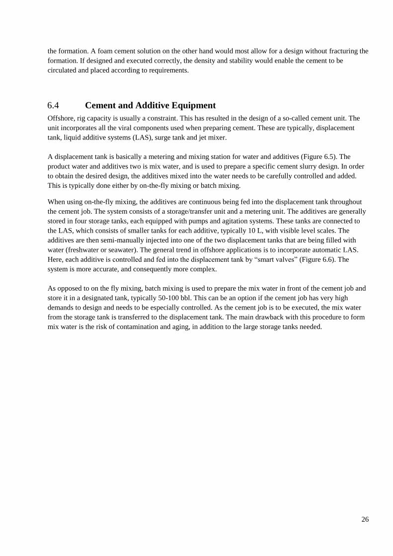
26

the formation. A foam cement solution on the other hand would most allow for a design without fracturing the

formation. If designed and executed correctly, the density and stability would enable the cement to be

circulated and placed according to requirements.

Cement and Additive Equipment 6.4

Offshore, rig capacity is usually a constraint. This has resulted in the design of a so-called cement unit. The

unit incorporates all the viral components used when preparing cement. These are typically, displacement

tank, liquid additive systems (LAS), surge tank and jet mixer.

A displacement tank is basically a metering and mixing station for water and additives (Figure 6.5). The

product water and additives two is mix water, and is used to prepare a specific cement slurry design. In order

to obtain the desired design, the additives mixed into the water needs to be carefully controlled and added.

This is typically done either by on-the-fly mixing or batch mixing.

When using on-the-fly mixing, the additives are continuous being fed into the displacement tank throughout

the cement job. The system consists of a storage/transfer unit and a metering unit. The additives are generally

stored in four storage tanks, each equipped with pumps and agitation systems. These tanks are connected to

the LAS, which consists of smaller tanks for each additive, typically 10 L, with visible level scales. The

additives are then semi-manually injected into one of the two displacement tanks that are being filled with

water (freshwater or seawater). The general trend in offshore applications is to incorporate automatic LAS.

Here, each additive is controlled and fed into the displacement tank by “smart valves” (Figure 6.6). The

system is more accurate, and consequently more complex.

As opposed to on the fly mixing, batch mixing is used to prepare the mix water in front of the cement job and

store it in a designated tank, typically 50-100 bbl. This can be an option if the cement job has very high

demands to design and needs to be especially controlled. As the cement job is to be executed, the mix water

from the storage tank is transferred to the displacement tank. The main drawback with this procedure to form

mix water is the risk of contamination and aging, in addition to the large storage tanks needed.

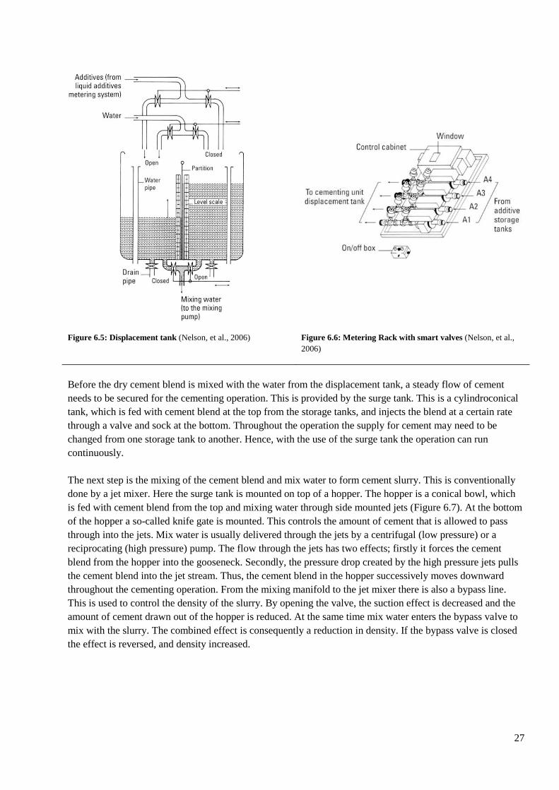
27

Figure 6.5: Displacement tank (Nelson, et al., 2006) Figure 6.6: Metering Rack with smart valves (Nelson, et al.,

2006)

Before the dry cement blend is mixed with the water from the displacement tank, a steady flow of cement

needs to be secured for the cementing operation. This is provided by the surge tank. This is a cylindroconical

tank, which is fed with cement blend at the top from the storage tanks, and injects the blend at a certain rate

through a valve and sock at the bottom. Throughout the operation the supply for cement may need to be

changed from one storage tank to another. Hence, with the use of the surge tank the operation can run

continuously.

The next step is the mixing of the cement blend and mix water to form cement slurry. This is conventionally

done by a jet mixer. Here the surge tank is mounted on top of a hopper. The hopper is a conical bowl, which

is fed with cement blend from the top and mixing water through side mounted jets (Figure 6.7). At the bottom

of the hopper a so-called knife gate is mounted. This controls the amount of cement that is allowed to pass

through into the jets. Mix water is usually delivered through the jets by a centrifugal (low pressure) or a

reciprocating (high pressure) pump. The flow through the jets has two effects; firstly it forces the cement

blend from the hopper into the gooseneck. Secondly, the pressure drop created by the high pressure jets pulls

the cement blend into the jet stream. Thus, the cement blend in the hopper successively moves downward

throughout the cementing operation. From the mixing manifold to the jet mixer there is also a bypass line.

This is used to control the density of the slurry. By opening the valve, the suction effect is decreased and the

amount of cement drawn out of the hopper is reduced. At the same time mix water enters the bypass valve to

mix with the slurry. The combined effect is consequently a reduction in density. If the bypass valve is closed

the effect is reversed, and density increased.

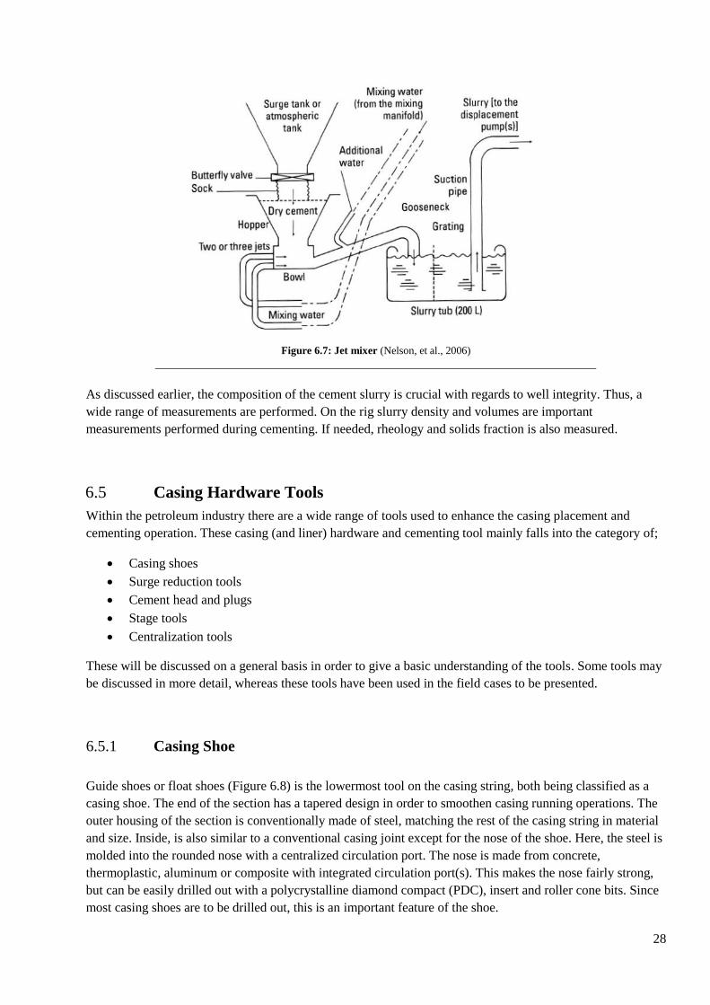
28

Figure 6.7: Jet mixer (Nelson, et al., 2006)

As discussed earlier, the composition of the cement slurry is crucial with regards to well integrity. Thus, a

wide range of measurements are performed. On the rig slurry density and volumes are important

measurements performed during cementing. If needed, rheology and solids fraction is also measured.

Casing Hardware Tools 6.5

Within the petroleum industry there are a wide range of tools used to enhance the casing placement and

cementing operation. These casing (and liner) hardware and cementing tool mainly falls into the category of;

Casing shoes

Surge reduction tools

Cement head and plugs

Stage tools

Centralization tools

These will be discussed on a general basis in order to give a basic understanding of the tools. Some tools may

be discussed in more detail, whereas these tools have been used in the field cases to be presented.

Casing Shoe 6.5.1

Guide shoes or float shoes (Figure 6.8) is the lowermost tool on the casing string, both being classified as a

casing shoe. The end of the section has a tapered design in order to smoothen casing running operations. The

outer housing of the section is conventionally made of steel, matching the rest of the casing string in material

and size. Inside, is also similar to a conventional casing joint except for the nose of the shoe. Here, the steel is

molded into the rounded nose with a centralized circulation port. The nose is made from concrete,

thermoplastic, aluminum or composite with integrated circulation port(s). This makes the nose fairly strong,

but can be easily drilled out with a polycrystalline diamond compact (PDC), insert and roller cone bits. Since

most casing shoes are to be drilled out, this is an important feature of the shoe.

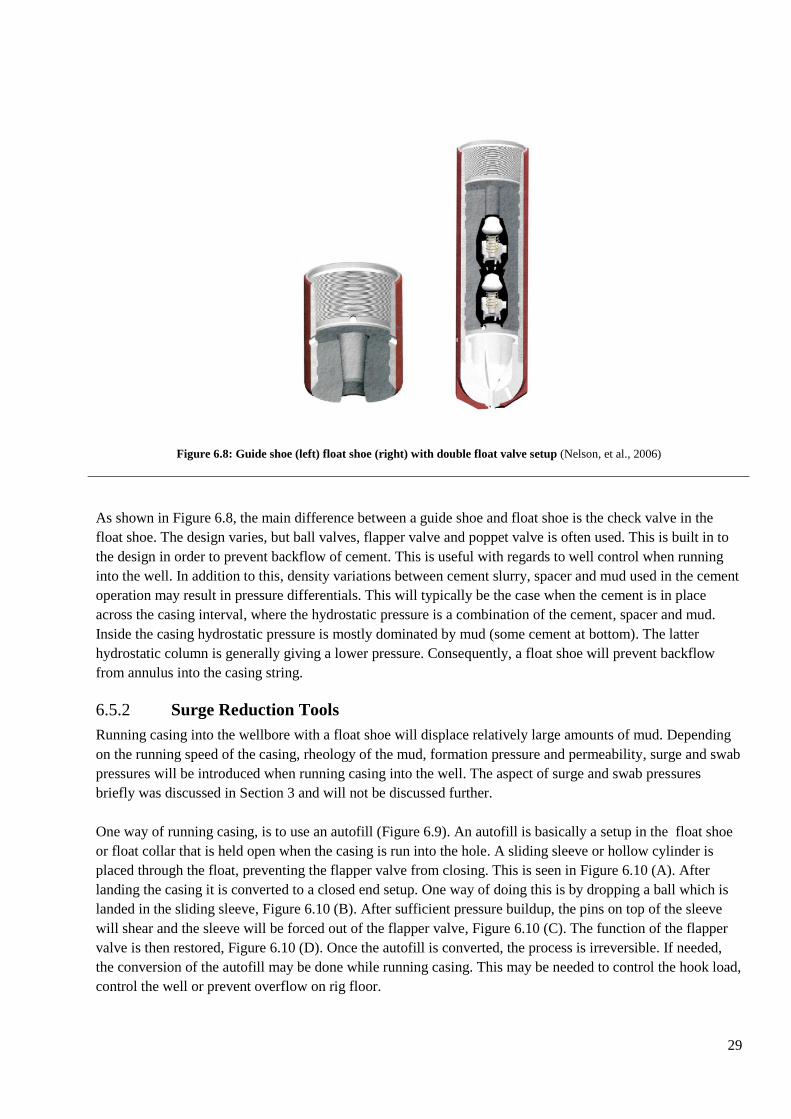
29

Figure 6.8: Guide shoe (left) float shoe (right) with double float valve setup (Nelson, et al., 2006)

As shown in Figure 6.8, the main difference between a guide shoe and float shoe is the check valve in the

float shoe. The design varies, but ball valves, flapper valve and poppet valve is often used. This is built in to

the design in order to prevent backflow of cement. This is useful with regards to well control when running

into the well. In addition to this, density variations between cement slurry, spacer and mud used in the cement

operation may result in pressure differentials. This will typically be the case when the cement is in place

across the casing interval, where the hydrostatic pressure is a combination of the cement, spacer and mud.

Inside the casing hydrostatic pressure is mostly dominated by mud (some cement at bottom). The latter

hydrostatic column is generally giving a lower pressure. Consequently, a float shoe will prevent backflow

from annulus into the casing string.

Surge Reduction Tools 6.5.2

Running casing into the wellbore with a float shoe will displace relatively large amounts of mud. Depending

on the running speed of the casing, rheology of the mud, formation pressure and permeability, surge and swab

pressures will be introduced when running casing into the well. The aspect of surge and swab pressures

briefly was discussed in Section 3 and will not be discussed further.

One way of running casing, is to use an autofill (Figure 6.9). An autofill is basically a setup in the float shoe

or float collar that is held open when the casing is run into the hole. A sliding sleeve or hollow cylinder is

placed through the float, preventing the flapper valve from closing. This is seen in Figure 6.10 (A). After

landing the casing it is converted to a closed end setup. One way of doing this is by dropping a ball which is

landed in the sliding sleeve, Figure 6.10 (B). After sufficient pressure buildup, the pins on top of the sleeve

will shear and the sleeve will be forced out of the flapper valve, Figure 6.10 (C). The function of the flapper

valve is then restored, Figure 6.10 (D). Once the autofill is converted, the process is irreversible. If needed,

the conversion of the autofill may be done while running casing. This may be needed to control the hook load,

control the well or prevent overflow on rig floor.

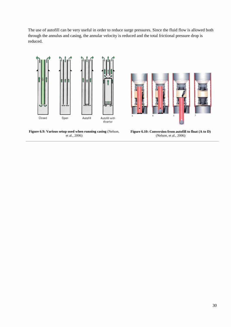
30

The use of autofill can be very useful in order to reduce surge pressures. Since the fluid flow is allowed both

through the annulus and casing, the annular velocity is reduced and the total frictional pressure drop is

reduced.

Figure 6.9: Various setup used when running casing (Nelson,

et al., 2006)

Figure 6.10: Conversion from autofill to float (A to D)

(Nelson, et al., 2006)

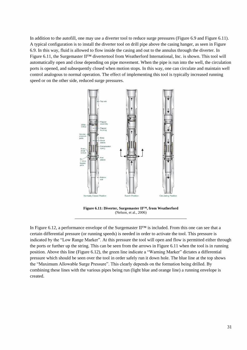
31

In addition to the autofill, one may use a diverter tool to reduce surge pressures (Figure 6.9 and Figure 6.11).

A typical configuration is to install the diverter tool on drill pipe above the casing hanger, as seen in Figure

6.9. In this way, fluid is allowed to flow inside the casing and out to the annulus through the diverter. In

Figure 6.11, the Surgemaster II™ divertertool from Weatherford International, Inc. is shown. This tool will

automatically open and close depending on pipe movement. When the pipe is run into the well, the circulation

ports is opened, and subsequently closed when motion stops. In this way, one can circulate and maintain well

control analogous to normal operation. The effect of implementing this tool is typically increased running

speed or on the other side, reduced surge pressures.

Figure 6.11: Diverter, Surgemaster II™, from Weatherford

(Nelson, et al., 2006)

In Figure 6.12, a performance envelope of the Surgemaster II™ is included. From this one can see that a

certain differential pressure (or running speeds) is needed in order to activate the tool. This pressure is

indicated by the “Low Range Marker”. At this pressure the tool will open and flow is permitted either through

the ports or further up the string. This can be seen from the arrows in Figure 6.11 when the tool is in running

position. Above this line (Figure 6.12), the green line indicate a “Warning Marker” dictates a differential

pressure which should be seen over the tool in order safely run it down hole. The blue line at the top shows

the “Maximum Allowable Surge Pressure”. This clearly depends on the formation being drilled. By

combining these lines with the various pipes being run (light blue and orange line) a running envelope is

created.

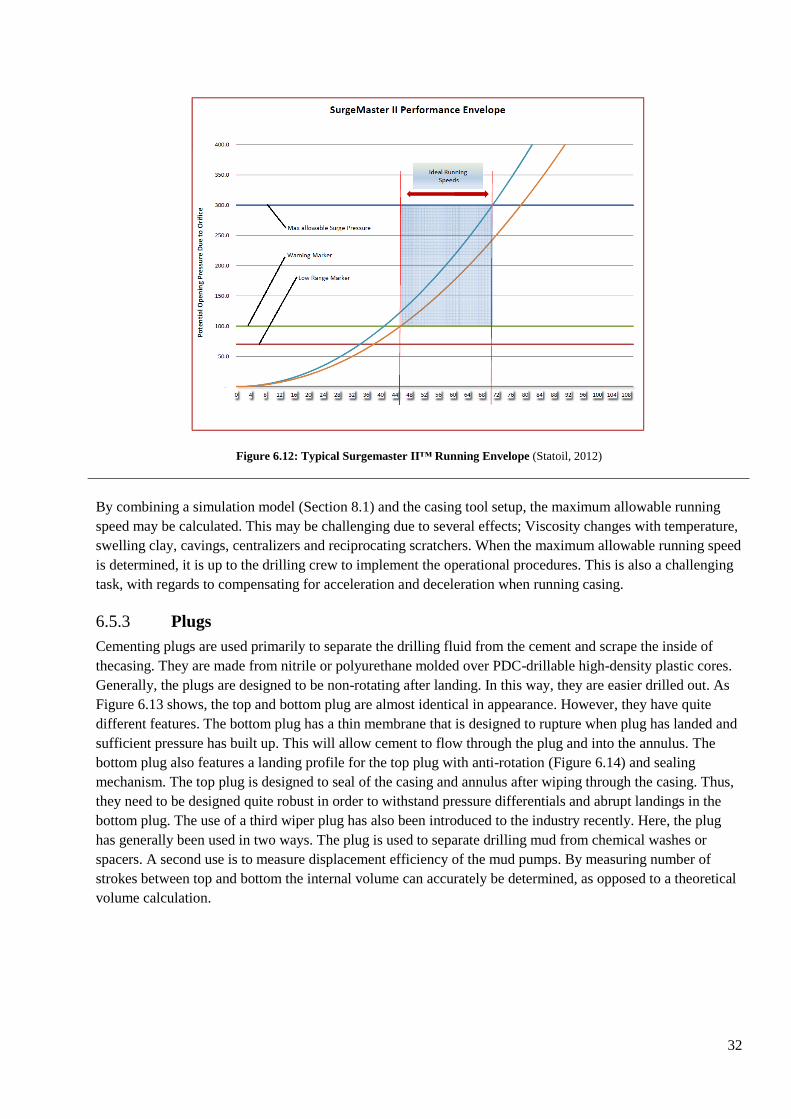
32

Figure 6.12: Typical Surgemaster II™ Running Envelope (Statoil, 2012)

By combining a simulation model (Section 8.1) and the casing tool setup, the maximum allowable running

speed may be calculated. This may be challenging due to several effects; Viscosity changes with temperature,

swelling clay, cavings, centralizers and reciprocating scratchers. When the maximum allowable running speed

is determined, it is up to the drilling crew to implement the operational procedures. This is also a challenging

task, with regards to compensating for acceleration and deceleration when running casing.

Plugs 6.5.3

Cementing plugs are used primarily to separate the drilling fluid from the cement and scrape the inside of

thecasing. They are made from nitrile or polyurethane molded over PDC-drillable high-density plastic cores.

Generally, the plugs are designed to be non-rotating after landing. In this way, they are easier drilled out. As

Figure 6.13 shows, the top and bottom plug are almost identical in appearance. However, they have quite

different features. The bottom plug has a thin membrane that is designed to rupture when plug has landed and

sufficient pressure has built up. This will allow cement to flow through the plug and into the annulus. The

bottom plug also features a landing profile for the top plug with anti-rotation (Figure 6.14) and sealing

mechanism. The top plug is designed to seal of the casing and annulus after wiping through the casing. Thus,

they need to be designed quite robust in order to withstand pressure differentials and abrupt landings in the

bottom plug. The use of a third wiper plug has also been introduced to the industry recently. Here, the plug

has generally been used in two ways. The plug is used to separate drilling mud from chemical washes or

spacers. A second use is to measure displacement efficiency of the mud pumps. By measuring number of

strokes between top and bottom the internal volume can accurately be determined, as opposed to a theoretical

volume calculation.

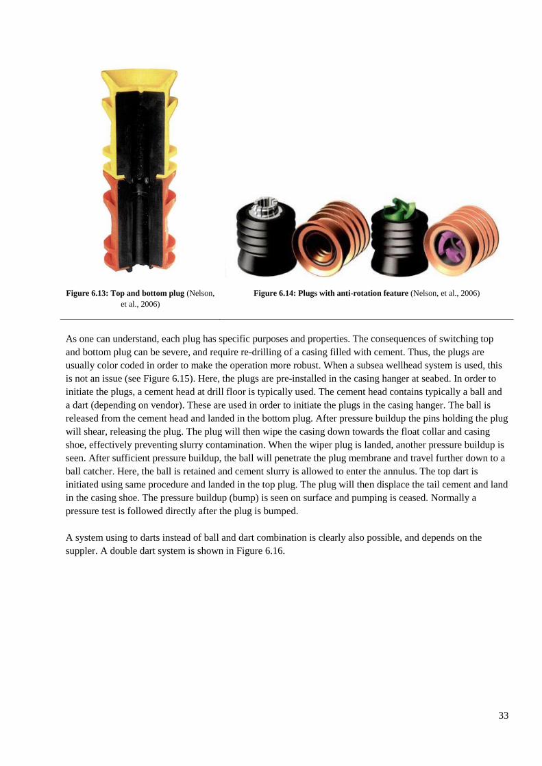
33

Figure 6.13: Top and bottom plug (Nelson,

et al., 2006) Figure 6.14: Plugs with anti-rotation feature (Nelson, et al., 2006)

As one can understand, each plug has specific purposes and properties. The consequences of switching top

and bottom plug can be severe, and require re-drilling of a casing filled with cement. Thus, the plugs are

usually color coded in order to make the operation more robust. When a subsea wellhead system is used, this

is not an issue (see Figure 6.15). Here, the plugs are pre-installed in the casing hanger at seabed. In order to

initiate the plugs, a cement head at drill floor is typically used. The cement head contains typically a ball and

a dart (depending on vendor). These are used in order to initiate the plugs in the casing hanger. The ball is

released from the cement head and landed in the bottom plug. After pressure buildup the pins holding the plug

will shear, releasing the plug. The plug will then wipe the casing down towards the float collar and casing

shoe, effectively preventing slurry contamination. When the wiper plug is landed, another pressure buildup is

seen. After sufficient pressure buildup, the ball will penetrate the plug membrane and travel further down to a

ball catcher. Here, the ball is retained and cement slurry is allowed to enter the annulus. The top dart is

initiated using same procedure and landed in the top plug. The plug will then displace the tail cement and land

in the casing shoe. The pressure buildup (bump) is seen on surface and pumping is ceased. Normally a

pressure test is followed directly after the plug is bumped.

A system using to darts instead of ball and dart combination is clearly also possible, and depends on the

suppler. A double dart system is shown in Figure 6.16.

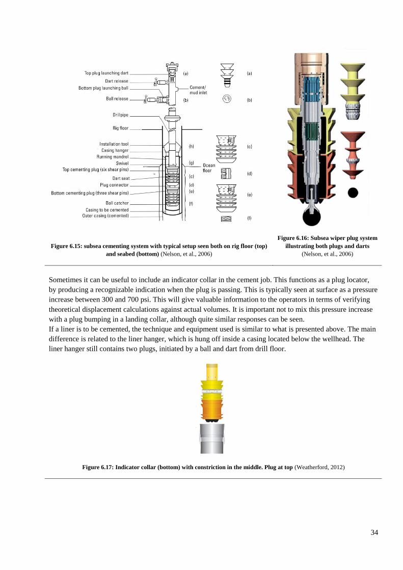
34

Figure 6.15: subsea cementing system with typical setup seen both on rig floor (top)

and seabed (bottom) (Nelson, et al., 2006)

Figure 6.16: Subsea wiper plug system

illustrating both plugs and darts

(Nelson, et al., 2006)

Sometimes it can be useful to include an indicator collar in the cement job. This functions as a plug locator,

by producing a recognizable indication when the plug is passing. This is typically seen at surface as a pressure

increase between 300 and 700 psi. This will give valuable information to the operators in terms of verifying

theoretical displacement calculations against actual volumes. It is important not to mix this pressure increase

with a plug bumping in a landing collar, although quite similar responses can be seen.

If a liner is to be cemented, the technique and equipment used is similar to what is presented above. The main

difference is related to the liner hanger, which is hung off inside a casing located below the wellhead. The

liner hanger still contains two plugs, initiated by a ball and dart from drill floor.

Figure 6.17: Indicator collar (bottom) with constriction in the middle. Plug at top (Weatherford, 2012)

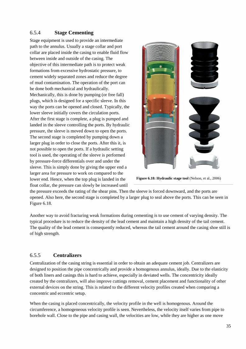
35

Stage Cementing 6.5.4

Stage equipment is used to provide an intermediate

path to the annulus. Usually a stage collar and port

collar are placed inside the casing to enable fluid flow

between inside and outside of the casing. The

objective of this intermediate path is to protect weak

formations from excessive hydrostatic pressure, to

cement widely separated zones and reduce the degree

of mud contamination. The operation of the port can

be done both mechanical and hydraulically.

Mechanically, this is done by pumping (or free fall)

plugs, which is designed for a specific sleeve. In this

way the ports can be opened and closed. Typically, the

lower sleeve initially covers the circulation ports.

After the first stage is complete, a plug is pumped and

landed in the sleeve controlling the ports. By hydraulic

pressure, the sleeve is moved down to open the ports.

The second stage is completed by pumping down a

larger plug in order to close the ports. After this it, is

not possible to open the ports. If a hydraulic setting

tool is used, the operating of the sleeve is performed

by pressure-force differentials over and under the

sleeve. This is simply done by giving the upper end a

larger area for pressure to work on compared to the

lower end. Hence, when the top plug is landed in the

float collar, the pressure can slowly be increased until

the pressure exceeds the rating of the shear pins. Then the sleeve is forced downward, and the ports are

opened. Also here, the second stage is completed by a larger plug to seal above the ports. This can be seen in

Figure 6.18.

Another way to avoid fracturing weak formations during cementing is to use cement of varying density. The

typical procedure is to reduce the density of the lead cement and maintain a high density of the tail cement.

The quality of the lead cement is consequently reduced, whereas the tail cement around the casing shoe still is

of high strength.

Centralizers 6.5.5

Centralization of the casing string is essential in order to obtain an adequate cement job. Centralizers are

designed to position the pipe concentrically and provide a homogenous annulus, ideally. Due to the elasticity

of both liners and casings this is hard to achieve, especially in deviated wells. The concentricity ideally

created by the centralizers, will also improve cuttings removal, cement placement and functionality of other

external devices on the string. This is related to the different velocity profiles created when comparing a

concentric and eccentric setup.

When the casing is placed concentrically, the velocity profile in the well is homogenous. Around the

circumference, a homogeneous velocity profile is seen. Nevertheless, the velocity itself varies from pipe to

borehole wall. Close to the pipe and casing wall, the velocities are low, while they are higher as one move

Figure 6.18: Hydraulic stage tool (Nelson, et al., 2006)

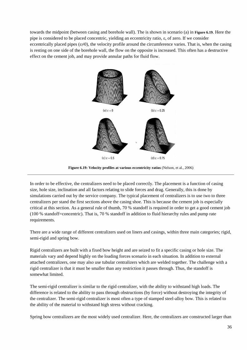
36

towards the midpoint (between casing and borehole wall). The is shown in scenario (a) in Figure 6.19. Here the

pipe is considered to be placed concentric, yielding an eccentricity ratio, ε, of zero. If we consider

eccentrically placed pipes (ε≠0), the velocity profile around the circumference varies. That is, when the casing

is resting on one side of the borehole wall, the flow on the opposite is increased. This often has a destructive

effect on the cement job, and may provide annular paths for fluid flow.

Figure 6.19: Velocity profiles at various eccentricity ratios (Nelson, et al., 2006)

In order to be effective, the centralizers need to be placed correctly. The placement is a function of casing

size, hole size, inclination and all factors relating to slide forces and drag. Generally, this is done by

simulations carried out by the service company. The typical placement of centralizers is to use two to three

centralizers per stand the first sections above the casing shoe. This is because the cement job is especially

critical at this section. As a general rule of thumb, 70 % standoff is required in order to get a good cement job

(100 % standoff=concentric). That is, 70 % standoff in addition to fluid hierarchy rules and pump rate

requirements.

There are a wide range of different centralizers used on liners and casings, within three main categories; rigid,

semi-rigid and spring bow.

Rigid centralizers are built with a fixed bow height and are seized to fit a specific casing or hole size. The

materials vary and depend highly on the loading forces scenario in each situation. In addition to external

attached centralizers, one may also use tubular centralizers which are welded together. The challenge with a

rigid centralizer is that it must be smaller than any restriction it passes through. Thus, the standoff is

somewhat limited.

The semi-rigid centralizer is similar to the rigid centralizer, with the ability to withstand high loads. The

difference is related to the ability to pass through obstructions (by force) without destroying the integrity of

the centralizer. The semi-rigid centralizer is most often a type of stamped steel-alloy bow. This is related to

the ability of the material to withstand high stress without cracking.

Spring bow centralizers are the most widely used centralizer. Here, the centralizers are constructed larger than

37

the hole in which they are run. Spring steel bows is the centralizing mechanism, where the design must be

stiff enough to efficiently place the pipe in the hole and still be flexible enough to be run into the hole.

In addition to these conventional centralizers, close-tolerance centralizers have also been designed to aid holes

with casing clearances less than 0.75 in. per side. This is clearly essential for deep water wells, as the

sensitivity towards centralization increases with decreasing clearance.

Wellbore Preparations 6.6

In order to get a successful cement job, several predefined steps are generally followed. After finishing

drilling, the well should be cleaned thoroughly. The objective in this phase is to remove remaining cuttings

and secure that the mud is in good condition. This is done by circulating the well. By circulating the well, the

temperature profile of the wellbore is also aimed to match the testing temperature of the cementing fluid.

Ideally, the mud should be replaced by fresh conditioned mud, containing the rheology properties required for

the cementing operation. Here, the mud should not be of higher rheology than the spacer and cement fluid,

also known as the rheology hierarchy rule. This is a fundamental requirement in order to obtain a successful

mud removal. Compatibility between the mud and cement is often poor, where mud will have a destructive

effect on the cement job if they are allowed to be mixed. Hence, displacement with mud and cement interface

is usually avoided by use of plugs (section 6.5). The same hierarchy is seen with regards to density of fluids in

the cement operation. That is, cement is of highest density and mud of lowest. This is desirable in order to

keep the cement in the bottom of the hole after it is placed. One consequence of this is free-fall of fluids in the

string. While pumping the heavier fluids, these will naturally tend to force the tighter fluid (mud) further

downhole in order to maintain the pressure equilibrium between the string and annulus. This will be a

dynamic interaction between density and rheology of the fluids. This will most likely lead to a varying flow

rate out of the well during the cement job, although the displacement rate is constant throughout the cement

job.

Cement Job 6.7

Here a typical cement job will be presented. The operation will be briefly run through and discussed. The

general procedure is as follows;

Pump spacer

Drop ball

Pump cement

Drop dart

Pump Spacer

Displace with mud (Rig pumps)

The cement unit starts by pumping the spacer and drops the ball in the cement head, which lands in the

bottom plug. After the (weighted) spacer is pumped, the cement unit starts pumping cement slurry and

subsequently drops the dart. The cement slurry and small volume of spacer are then displaced by the rig

pumps with mud down the string. The cement is then displaced through the bottom plug, out the casing shoe

and up into the annulus. The mud displacement volumes needed in order to place the cement correctly is

calculated and correlated with strokes on the pumps. This is conditioned that the calculated stokes matches

actual strokes in order to displace the cement to a specific depth.

In front of the cement job, simulations are generally performed. Provided high quality input data, This will

most likely simplify the fluid design and provide indications of what one can expect in terms of operation

38

requirements. It is especially important to maintain a sufficient circulation rate when the cement is being

placed. If encountering losses during a cement job and planned circulations cannot be achieved, testing should

be initiated to validate the cement job. Losses during a cement job can be planned. The important question

here is where the actual loss zone is. If the loss zone is located above top of cement, TOC, loss of returns will

be seen at surface although an adequate cement job is performed. On the other hand if the loss zone is located

between TOC and the casing shoe, the cement job will be affected. Thus, it is very useful to know where the

loss zone is. This is generally a challenging task, but one can use the pump pressure of the cement

displacement pumps to determine where the cement is when losses are encountered. As the cement exit the

shoe and enters the annulus the pump pressure tend to increase (dcem>dspacer), indicating that the cement has

entered the annulus.

The most important paramteters in a cement job can be summed up by:

Flow rate

o Minimum restriction to secure proper cement displacement

o Maximum restriction with regards to ECD

Fluid design

o Additived

o Volumes

Centralization

Cement Testing 6.8

After performing the primary cement job the cement is usually evaluated by pressure testing or logging tools.

Pressure testing is the most common method. In order not to damage the set cement or cement/casing bond it

is usually performed after the cement is set. After the cement is set the shoe is drilled out and a

FIT/LOT/XLOT performed to confirm drillability of the next section. If the casing shoe does not hold the

planned pressure, a remedial cementing operation is required. The important thing is to maintain well integrity

(Nelson, et al., 2006).

Consequenses of a Poor Cement Job 6.9

A classic scenario of the potential consequences of a poor cement job is the the Macondo blowout 20/04/2012

(BP, 2010). The Macondo well was a deepwater (~1500 m) exploration well, with a 36” - 28” - 22” - 16” - 13

5/8” - 11 7/8” - 9 7/8” casing design. The Deepwater Horizon drilling rig had recently reached target depth

after several remedial cementing operations and a side track. The subsequent logging indicated the presence

of hydrocarbons, and the well was decided plugged and abandoned (Transocean, 2012). Here, BP suggests

that the foam cement was unable to provide well integrity and seal the wellbore against hydrocarbons. That is,

the foam design was unable to generate stable foam cement sealing against the hydrocarbons. This key well

integrity failure and seven other steps, illustrated in Figure 6.20, subsequently led to the fatal incident

claiming the life of 11 workers.

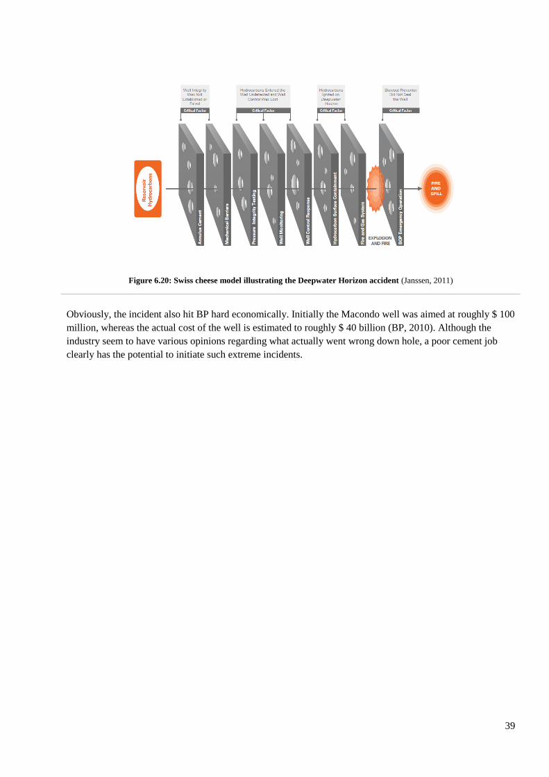
39

Obviously, the incident also hit BP hard economically. Initially the Macondo well was aimed at roughly $ 100

million, whereas the actual cost of the well is estimated to roughly $ 40 billion (BP, 2010). Although the

industry seem to have various opinions regarding what actually went wrong down hole, a poor cement job

clearly has the potential to initiate such extreme incidents.

Figure 6.20: Swiss cheese model illustrating the Deepwater Horizon accident (Janssen, 2011)

40

Requirements 7

Requirements are in some sense split into two legislatives. The first one is considered to be the local

requirements found at the specific area to be drilled. This is requirements given by the local authorities, and

varies to a large extent around the world. Typically, if one were to drill a well in the GoM, on would have to

comply to the requirements given in the Code of Federal Regulations (Office of the Federal Register, 2011) in

order to get a so-called “license to drill”. The second requirements one needs to comply to, are the ones

dictated by the company responsible of drilling the well. In Statoil, this management system is called ARIS.

Both these legislatives need to be implemented and followed. If a requirement from ARIS surpasses a local

requirement, ARIS requirement will be apply and vice versa.

Drilling Fluid Requirements 7.1

Generally there is also added a safety margin to the fluid in the borehole. This safety factor is governed by

riser margin, trip margin, compressibility of the fluid and other factors affecting the equivalent mud weight,

EMW. Riser margin is simply the extra mud weight needed in order to keep the well overbalanced although

riser is removed. This may typically be a riser emergency disconnect from the BOP due to rough weather. The

consequence of this is mud being replaced by seawater from seabed to sea level. Clearly, this effect is

amplified with increasing water depth, and is often not achievable in deepwater drilling. Thus, in Statoil this

would require the drilling engineer to apply for a deviation when planning this well in ARIS. The situation

would then be evaluated, and either approved or rejected. The operational consequence of the inability to

provide riser margin is special procedures when disconnecting the BOP. That is, in order to maintain

overbalance, the BOP is shut in with a certain pressure.

Trip margin is related to the extra mud weight needed in order to keep the well overbalanced although the

pressure may be reduced by swabbing. Also here the effect is generally amplified with depth due to the low

clearances seen between the casing strings.

The compressibility of the drilling fluid is also complex and depends highly on fluid composition. That is, oil

based muds are generally more compressible than water based muds and may pose challenges due to the large

pressures encountered in deepwater drilling. Another aspect of fluid compressibility is the dependency of

temperature. At seabed the temperatures approach 0°C, and as one moves further downhole the temperature

gradient is altered from negative to positive. This effect can be quite complex, but the general trend is

decreased density with increasing temperature (Aadnøy, 1998; Wikipedia, 2012).

Cementing Requirements 7.2

Cementing the annulus after reaching target depth of the section is critical for the integrity of the well.

Requirements are implemented in order to fulfill the objectives of zonal isolation and structural support of the

casing (or liner). The requirements of the cement operation depend on which section is being drilled.

ARIS require 100 m cement column above casing shoe. If a casing shoe is not to be drilled out, a cement

column of 200m is required above the point of potential flow/leakage point/permeable formation of

hydrocarbons.

As for the GoM, the requirements related to be found in the CFR (Office of the Federal Register, 2011). Some

of these are presented below:

41

Conductor is required to be cemented to seabed

The surface casing is required to be cemented at least 200 ft into the conductor casing (based on

calculated volumes) and to seabed if fractures or faults exists.

For intermediate casings and production casings (including liners) it is required to use enough cement

to cover and isolate 500 ft above all hydrocarbon-bearing zones and isolate abnormal pressure

intervals from normal pressure intervals. As a minimum it is required to cement 500 ft above the

casing shoe if no abnormal pressures or hydrocarbon zones are encountered

The main objectives in are nevertheless zonal isolation and structural support (Statoil ARIS, 2012).

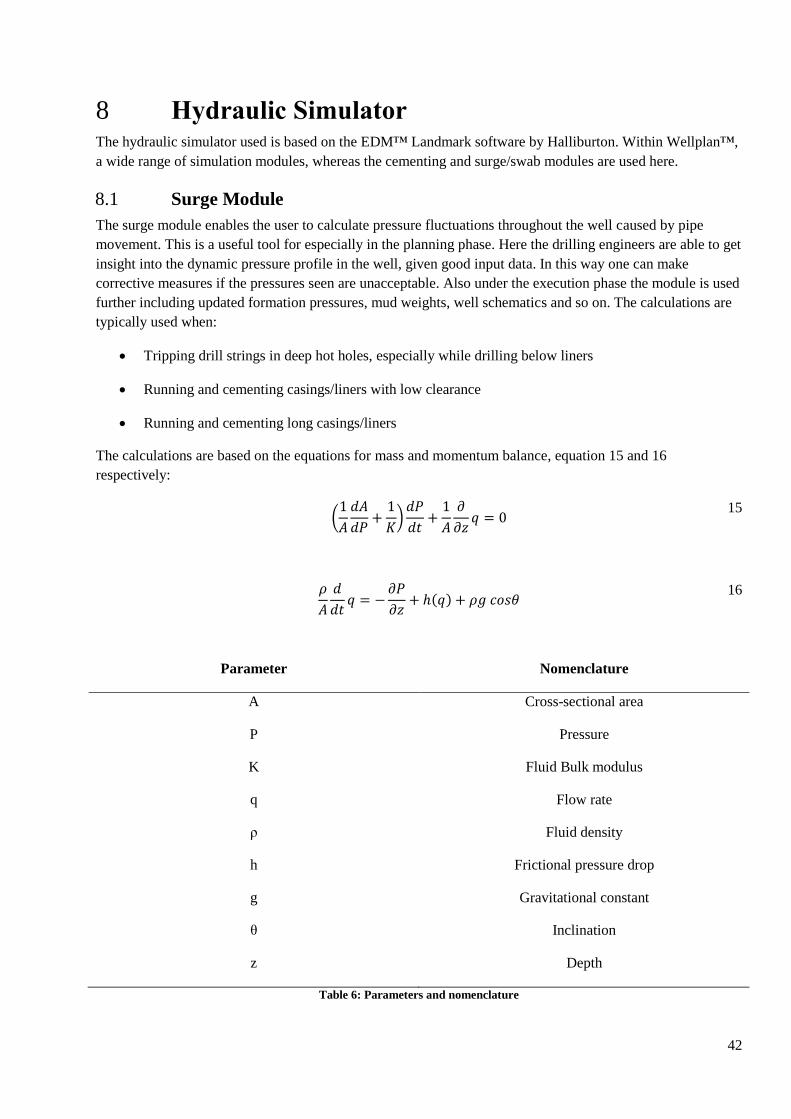
42

Hydraulic Simulator 8The hydraulic simulator used is based on the EDM™ Landmark software by Halliburton. Within Wellplan™,

a wide range of simulation modules, whereas the cementing and surge/swab modules are used here.

Surge Module 8.1

The surge module enables the user to calculate pressure fluctuations throughout the well caused by pipe

movement. This is a useful tool for especially in the planning phase. Here the drilling engineers are able to get

insight into the dynamic pressure profile in the well, given good input data. In this way one can make

corrective measures if the pressures seen are unacceptable. Also under the execution phase the module is used

further including updated formation pressures, mud weights, well schematics and so on. The calculations are

typically used when:

Tripping drill strings in deep hot holes, especially while drilling below liners

Running and cementing casings/liners with low clearance

Running and cementing long casings/liners

The calculations are based on the equations for mass and momentum balance, equation 15 and 16

respectively:

(

)

15

16

Parameter Nomenclature

A Cross-sectional area

P Pressure

K Fluid Bulk modulus

q Flow rate

ρ Fluid density

h Frictional pressure drop

g Gravitational constant

θ Inclination

z Depth

Table 6: Parameters and nomenclature

43

The equation of mass balance basically says that matter cannot disappear or be created spontaneously

(Wikipedia, 2012). That is, conservation of mass. By accounting for material entering and leaving a system,

mass flows can be identified.

The equation of momentum balance considers the forces acting on the system and in the system. This balance

is governed by the fact that if no external force acts on a closed system, the momentum of the closed system

remains constant (Wikipedia, 2012).

The calculations are divided into two sections. One from pipe top to bottom and the other one form pipe

bottom to bottom of hole. By use of interpolation each pressure point can be calculated from a boundary

condition at a specific time. In order to include the dynamic aspect, a new calculation is performed at a time

∆t after the preceding calculation. Since waves move with the speed of sound in the matter it is travelling, the

time intervals has a minimum/Maximum value. The time steps can be adjusted to a minimum/maximum from

the time it takes a sound wave to travel through a specific interval of calculation. This means that for a

saltwater (c=1500m/s) section of 10 meters, tmin= 0.0067 s. In this way the user may specify intervals of

special interest, where the time steps is shortened in ordered to give good dynamic resolution and vice versa.

This can be especially interesting around the bit when tripping into a small clearance hole.

Cementing Module 8.2

The cementing module can be used in order to predict pressure fluctuations during cementing operations. This

is especially useful in order to optimize cementing operations and avoiding expensive remedial cementing.

The typical scenarios include:

Safe pump rates

Surface pressure

Downhole pressures

Nitrogen concentration

Downhole rheology

Temperature thinning of fluids

The exact equations are somewhat limited given by the Landmark software. Clearly, the model is relatively

advanced and becomes even more complex when one considers the compressibility of fluids in a dynamic

picture. As discussed in section 6.3, there does not seem to be a general set of accepted models and equations

for calculating the multiphase flow of cement.

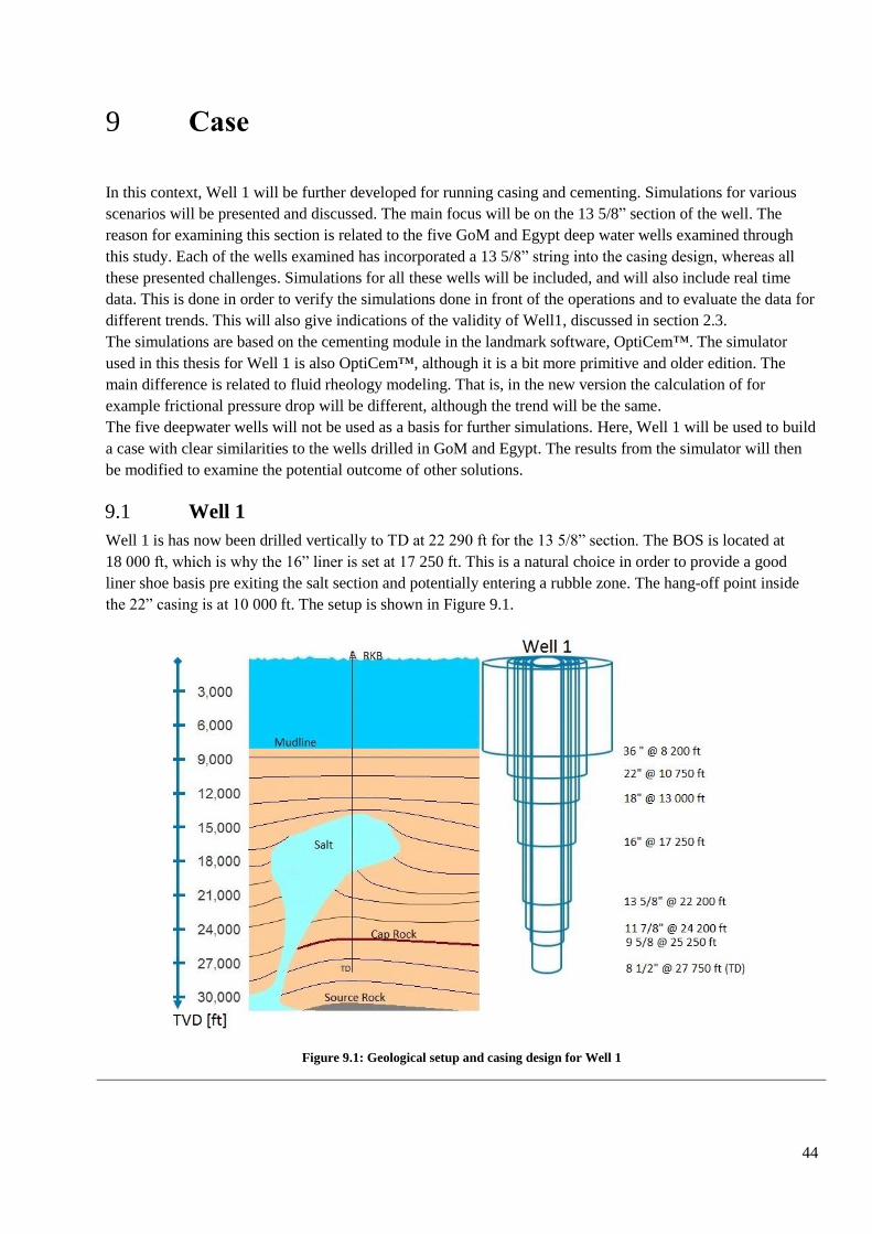
44

Case 9

In this context, Well 1 will be further developed for running casing and cementing. Simulations for various

scenarios will be presented and discussed. The main focus will be on the 13 5/8” section of the well. The

reason for examining this section is related to the five GoM and Egypt deep water wells examined through

this study. Each of the wells examined has incorporated a 13 5/8” string into the casing design, whereas all

these presented challenges. Simulations for all these wells will be included, and will also include real time

data. This is done in order to verify the simulations done in front of the operations and to evaluate the data for

different trends. This will also give indications of the validity of Well1, discussed in section 2.3.

The simulations are based on the cementing module in the landmark software, OptiCem™. The simulator

used in this thesis for Well 1 is also OptiCem™, although it is a bit more primitive and older edition. The

main difference is related to fluid rheology modeling. That is, in the new version the calculation of for

example frictional pressure drop will be different, although the trend will be the same.

The five deepwater wells will not be used as a basis for further simulations. Here, Well 1 will be used to build

a case with clear similarities to the wells drilled in GoM and Egypt. The results from the simulator will then

be modified to examine the potential outcome of other solutions.

Well 1 9.1

Well 1 is has now been drilled vertically to TD at 22 290 ft for the 13 5/8” section. The BOS is located at

18 000 ft, which is why the 16” liner is set at 17 250 ft. This is a natural choice in order to provide a good

liner shoe basis pre exiting the salt section and potentially entering a rubble zone. The hang-off point inside

the 22” casing is at 10 000 ft. The setup is shown in Figure 9.1.

Figure 9.1: Geological setup and casing design for Well 1

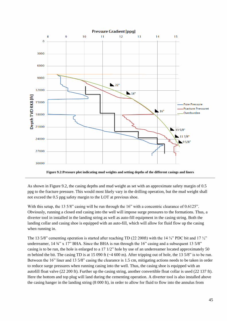
45

Figure 9.2:Pressure plot indicating mud weights and setting depths of the different casings and liners

As shown in Figure 9.2, the casing depths and mud weight as set with an approximate safety margin of 0.5

ppg to the fracture pressure. This would most likely vary in the drilling operation, but the mud weight shall

not exceed the 0.5 ppg safety margin to the LOT at previous shoe.

With this setup, the 13 5/8” casing will be run through the 16” with a concentric clearance of 0.6125”.

Obviously, running a closed end casing into the well will impose surge pressures to the formations. Thus, a

diverter tool in installed in the landing string as well as auto-fill equipment in the casing string. Both the

landing collar and casing shoe is equipped with an auto-fill, which will allow for fluid flow up the casing

when running in.

The 13 5/8” cementing operation is started after reaching TD (22 200ft) with the 14 ¾” PDC bit and 17 ½”

underreamer, 14 ¾” x 17” BHA. Since the BHA is run through the 16” casing and a subsequent 13 5/8”

casing is to be run, the hole is enlarged to a 17 1/2” hole by use of an underreamer located approximately 50

m behind the bit. The casing TD is at 15 090 ft (~4 600 m). After tripping out of hole, the 13 5/8” is to be run.

Between the 16” liner and 13 5/8” casing the clearance is 1.5 cm, mitigating actions needs to be taken in order

to reduce surge pressures when running casing into the well. Thus, the casing shoe is equipped with an

autofill float valve (22 200 ft). Further up the casing string, another convertible float collar is used (22 137 ft).

Here the bottom and top plug will land during the cementing operation. A diverter tool is also installed above

the casing hanger in the landing string (8 000 ft), in order to allow for fluid to flow into the annulus from

46

inside the string. Both these tool are discussed in section 6.5.2, and will help reduce the surge pressures

created when running into the well. The setup is summarized by in Figure 9.3.

Figure 9.3: String setup Well 1

Furthermore, centralizers are needed in order to maintain concentricity in the wellbore. The need for

centralizers will increase with increasing inclination in the well. Since this is considered a vertical exploration

well, the need heavy centralizer concentration is limited. Nevertheless, centralizers are required in order to

obtain the minimum requirement of 70 % standoff in the wellbore. As discussed in Section 6.5.5, centralizers

are essential to achieve cement all around the pipe, and therefore giving a hydraulic seal and zonal isolation.

Thus, centralization will be built in to 75 % in the simulations.

The section is planned to be cemented with a 1 000 ft cement column. This is due to the requirement of 500 ft

cement column above casing shoe or abnormal/hydrocarbon zone (Office of the Federal Register, 2011). With

a 1 000 ft cement column, thorough isolation is likely to be secured, and the required interval of 500 ft is less

prone to contamination. The cement slurry will be based on conventional cement slurry design. The reason for

not choosing foamed cement is due to:

Relatively short interval of cement (~1 000 ft)

Less logistics

More economical

More robust system

High cement slurry strength

In order to minimize losses when displacing the cementing, it would also generally be necessary to give

restrictions to pump rate. This is also something that will be based on simulations, and a typical value could

be 4-6 bbls/min (~600-1 000 L/min). This value also needs to be evaluated with respect to annular velocity

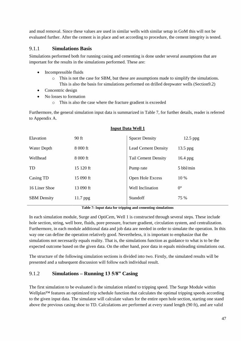
47

and mud removal. Since these values are used in similar wells with similar setup in GoM this will not be

evaluated further. After the cement is in place and set according to procedure, the cement integrity is tested.

Simulations Basis 9.1.1

Simulations performed both for running casing and cementing is done under several assumptions that are

important for the results in the simulations performed. These are:

Incompressible fluids

o This is not the case for SBM, but these are assumptions made to simplify the simulations.

This is also the basis for simulations performed on drilled deepwater wells (Section9.2)

Concentric design

No losses to formation

o This is also the case where the fracture gradient is exceeded

Furthermore, the general simulation input data is summarized in Table 7, for further details, reader is referred

to Appendix A.

Input Data Well 1

Elavation 90 ft Spacer Density 12.5 ppg

Water Depth 8 000 ft Lead Cement Density 13.5 ppg

Wellhead 8 000 ft Tail Cement Density 16.4 ppg

TD 15 120 ft Pump rate 5 bbl/min

Casing TD 15 090 ft Open Hole Excess 10 %

16 Liner Shoe 13 090 ft Well Inclination 0°

SBM Density 11.7 ppg Standoff 75 %

Table 7: Input data for tripping and cementing simulations

In each simulation module, Surge and OptiCem, Well 1 is constructed through several steps. These include

hole section, string, well bore, fluids, pore pressure, fracture gradient, circulation system, and centralization.

Furthermore, in each module additional data and job data are needed in order to simulate the operation. In this

way one can define the operation relatively good. Nevertheless, it is important to emphasize that the

simulations not necessarily equals reality. That is, the simulations function as guidance to what is to be the

expected outcome based on the given data. On the other hand, poor data in equals misleading simulations out.

The structure of the following simulation sections is divided into two. Firstly, the simulated results will be

presented and a subsequent discussion will follow each individual result.

Simulations – Running 13 5/8” Casing 9.1.2

The first simulation to be evaluated is the simulation related to tripping speed. The Surge Module within

Wellplan™ features an optimized trip schedule function that calculates the optimal tripping speeds according

to the given input data. The simulator will calculate values for the entire open hole section, starting one stand

above the previous casing shoe to TD. Calculations are performed at every stand length (90 ft), and are valid

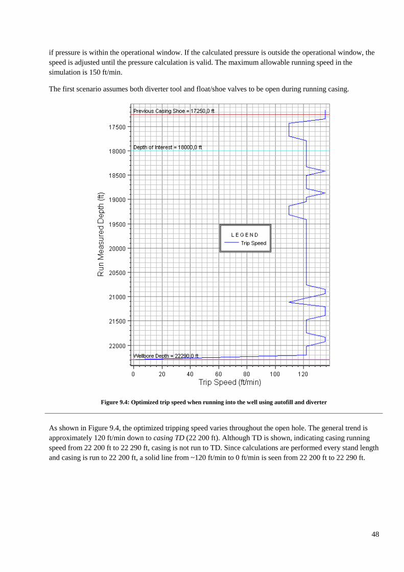
48

if pressure is within the operational window. If the calculated pressure is outside the operational window, the

speed is adjusted until the pressure calculation is valid. The maximum allowable running speed in the

simulation is 150 ft/min.

The first scenario assumes both diverter tool and float/shoe valves to be open during running casing.

Figure 9.4: Optimized trip speed when running into the well using autofill and diverter

As shown in Figure 9.4, the optimized tripping speed varies throughout the open hole. The general trend is

approximately 120 ft/min down to casing TD (22 200 ft). Although TD is shown, indicating casing running

speed from 22 200 ft to 22 290 ft, casing is not run to TD. Since calculations are performed every stand length

and casing is run to 22 200 ft, a solid line from ~120 ft/min to 0 ft/min is seen from 22 200 ft to 22 290 ft.

49

Figure 9.5: Maximum and minimum equivalent mud weights seen when running into the well with open float collar and

diverter

According to Figure 9.5, the maximum and minimum EMWs fluctuate approximately between 11.55 and

11.80 ppg. This means that both surge and swab are seen through the section. The maximum EMW at 18 000

ft (BOS) is approximately 0.3 ppg from the fracture pressure at this point. Thus, one would expect the

optimized tripping speed to be higher than what is presented in Figure 9.4. This is not the case. At TD the

pore pressure is 11.54 ppg and seem to equal the maximum and minimum EMWs. This implies that swabbing

is seen at this point since the mudweight is set to 11.70 ppg. When increasing the running speed to 130 ft/min

(Figure 9.6), swabbing pressures below the pore pressure is seen. With respect to hole integrity and

operational safety, this is not a desired scenario.

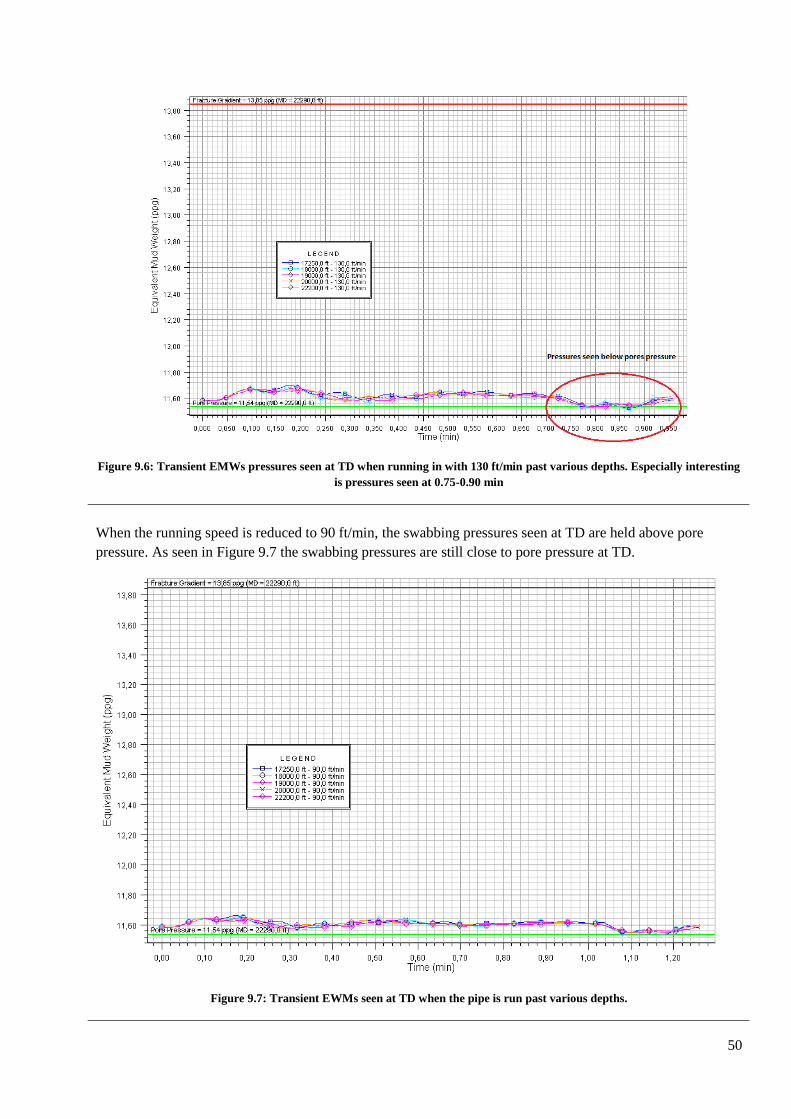
50

Figure 9.6: Transient EMWs pressures seen at TD when running in with 130 ft/min past various depths. Especially interesting

is pressures seen at 0.75-0.90 min

When the running speed is reduced to 90 ft/min, the swabbing pressures seen at TD are held above pore

pressure. As seen in Figure 9.7 the swabbing pressures are still close to pore pressure at TD.

Figure 9.7: Transient EWMs seen at TD when the pipe is run past various depths.

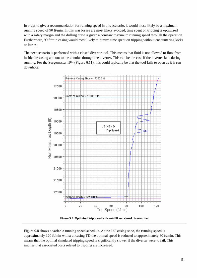
51

In order to give a recommendation for running speed in this scenario, it would most likely be a maximum

running speed of 90 ft/min. In this was losses are most likely avoided, time spent on tripping is optimized

with a safety margin and the drilling crew is given a constant maximum running speed through the operation.

Furthermore, 90 ft/min casing would most likely minimize time spent on tripping without encountering kicks

or losses.

The next scenario is performed with a closed diverter tool. This means that fluid is not allowed to flow from

inside the casing and out to the annulus through the diverter. This can be the case if the diverter fails during

running. For the Surgemaster II™ (Figure 6.11), this could typically be that the tool fails to open as it is run

downhole.

Figure 9.8: Optimized trip speed with autofill and closed diverter tool

Figure 9.8 shows a variable running speed schedule. At the 16” casing shoe, the running speed is

approximately 120 ft/min whilst at casing TD the optimal speed is reduced to approximately 80 ft/min. This

means that the optimal simulated tripping speed is significantly slower if the diverter were to fail. This

implies that associated costs related to tripping are increased.

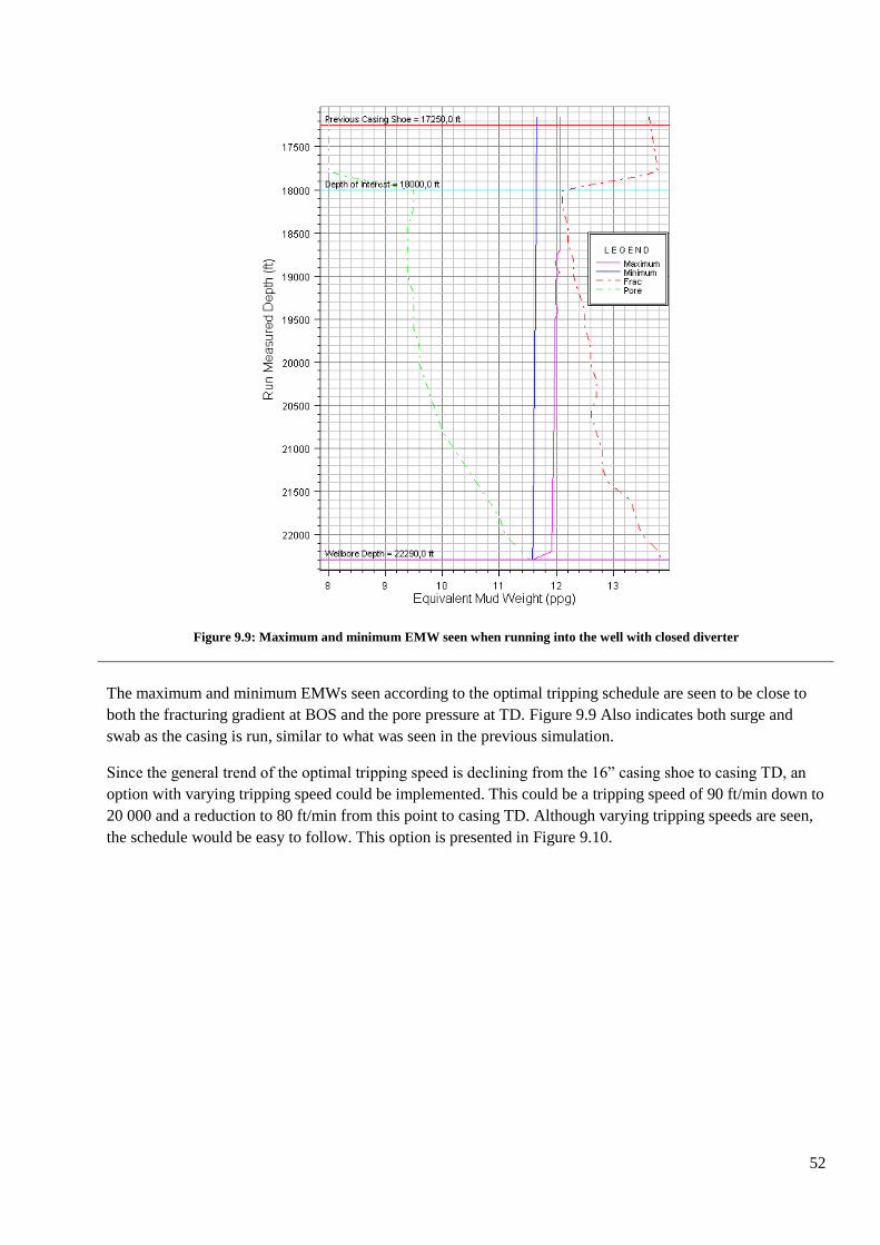
52

Figure 9.9: Maximum and minimum EMW seen when running into the well with closed diverter

The maximum and minimum EMWs seen according to the optimal tripping schedule are seen to be close to

both the fracturing gradient at BOS and the pore pressure at TD. Figure 9.9 Also indicates both surge and

swab as the casing is run, similar to what was seen in the previous simulation.

Since the general trend of the optimal tripping speed is declining from the 16” casing shoe to casing TD, an

option with varying tripping speed could be implemented. This could be a tripping speed of 90 ft/min down to

20 000 and a reduction to 80 ft/min from this point to casing TD. Although varying tripping speeds are seen,

the schedule would be easy to follow. This option is presented in Figure 9.10.

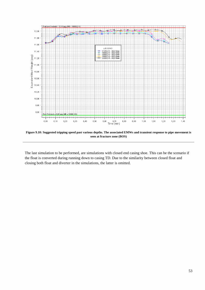
53

Figure 9.10: Suggested tripping speed past various depths. The associated EMWs and transient response to pipe movement is

seen at fracture zone (BOS)

The last simulation to be performed, are simulations with closed end casing shoe. This can be the scenario if

the float is converted during running down to casing TD. Due to the similarity between closed float and

closing both float and diverter in the simulations, the latter is omitted.

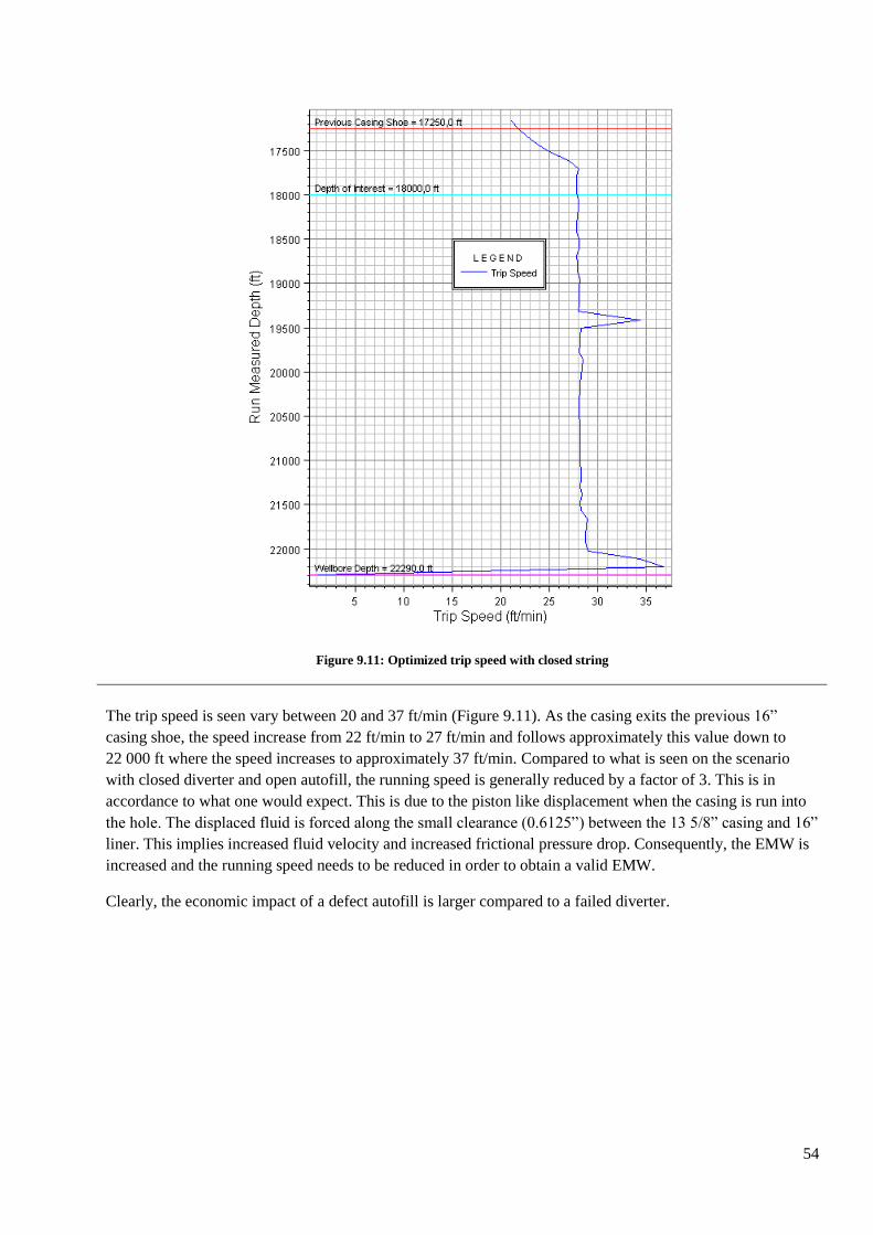
54

Figure 9.11: Optimized trip speed with closed string

The trip speed is seen vary between 20 and 37 ft/min (Figure 9.11). As the casing exits the previous 16”

casing shoe, the speed increase from 22 ft/min to 27 ft/min and follows approximately this value down to

22 000 ft where the speed increases to approximately 37 ft/min. Compared to what is seen on the scenario

with closed diverter and open autofill, the running speed is generally reduced by a factor of 3. This is in

accordance to what one would expect. This is due to the piston like displacement when the casing is run into

the hole. The displaced fluid is forced along the small clearance (0.6125”) between the 13 5/8” casing and 16”

liner. This implies increased fluid velocity and increased frictional pressure drop. Consequently, the EMW is

increased and the running speed needs to be reduced in order to obtain a valid EMW.

Clearly, the economic impact of a defect autofill is larger compared to a failed diverter.

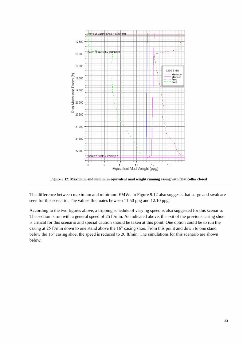
55

Figure 9.12: Maximum and minimum equivalent mud weight running casing with float collar closed

The difference between maximum and minimum EMWs in Figure 9.12 also suggests that surge and swab are

seen for this scenario. The values fluctuates beween 11.50 ppg and 12.10 ppg.

According to the two figures above, a tripping schedule of varying speed is also suggested for this scenario.

The section is run with a general speed of 25 ft/min. As indicated above, the exit of the previous casing shoe

is critical for this scenario and special caution should be taken at this point. One option could be to run the

casing at 25 ft/min down to one stand above the 16” casing shoe. From this point and down to one stand

below the 16” casing shoe, the speed is reduced to 20 ft/min. The simulations for this scenario are shown

below.

56

Figure 9.13: Transient response plot with reduced running speed at 16” casing shoe

As shown in Figure 9.13, fracturing is avoided if the running speed is reduced at casing shoe. A more detailed

simulation showing reduced running speeds one stand above and below the 16” casing shoe is shown below.

Figure 9.14: Transient response plot with reduced running speeds as suggested

Based on the optimized tripping schedule simulations for the various scenarios, the suggested running speeds

for the three different scenarios are shown in Table 8.

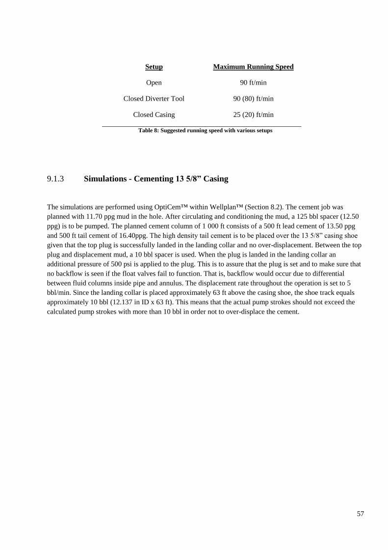
57

Setup Maximum Running Speed

Open 90 ft/min

Closed Diverter Tool 90 (80) ft/min

Closed Casing 25 (20) ft/min

Table 8: Suggested running speed with various setups

Simulations - Cementing 13 5/8” Casing 9.1.3

The simulations are performed using OptiCem™ within Wellplan™ (Section 8.2). The cement job was

planned with 11.70 ppg mud in the hole. After circulating and conditioning the mud, a 125 bbl spacer (12.50

ppg) is to be pumped. The planned cement column of 1 000 ft consists of a 500 ft lead cement of 13.50 ppg

and 500 ft tail cement of 16.40ppg. The high density tail cement is to be placed over the 13 5/8” casing shoe

given that the top plug is successfully landed in the landing collar and no over-displacement. Between the top

plug and displacement mud, a 10 bbl spacer is used. When the plug is landed in the landing collar an

additional pressure of 500 psi is applied to the plug. This is to assure that the plug is set and to make sure that

no backflow is seen if the float valves fail to function. That is, backflow would occur due to differential

between fluid columns inside pipe and annulus. The displacement rate throughout the operation is set to 5

bbl/min. Since the landing collar is placed approximately 63 ft above the casing shoe, the shoe track equals

approximately 10 bbl (12.137 in ID x 63 ft). This means that the actual pump strokes should not exceed the

calculated pump strokes with more than 10 bbl in order not to over-displace the cement.

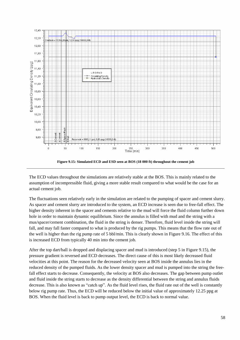
58

Figure 9.15: Simulated ECD and ESD seen at BOS (18 000 ft) throughout the cement job

The ECD values throughout the simulations are relatively stable at the BOS. This is mainly related to the

assumption of incompressible fluid, giving a more stable result compared to what would be the case for an

actual cement job.

The fluctuations seen relatively early in the simulation are related to the pumping of spacer and cement slurry.

As spacer and cement slurry are introduced to the system, an ECD increase is seen due to free-fall effect. The

higher density inherent in the spacer and cements relative to the mud will force the fluid column further down

hole in order to maintain dynamic equilibrium. Since the annulus is filled with mud and the string with a

mus/spacer/cement combination, the fluid in the string is denser. Therefore, fluid level inside the string will

fall, and may fall faster compared to what is produced by the rig pumps. This means that the flow rate out of

the well is higher than the rig pump rate of 5 bbl/min. This is clearly shown in Figure 9.16. The effect of this

is increased ECD from typically 40 min into the cement job.

After the top dart/ball is dropped and displacing spacer and mud is introduced (step 5 in Figure 9.15), the

pressure gradient is reversed and ECD decreases. The direct cause of this is most likely decreased fluid

velocities at this point. The reason for the decreased velocity seen at BOS inside the annulus lies in the

reduced density of the pumped fluids. As the lower density spacer and mud is pumped into the string the free-

fall effect starts to decrease. Consequently, the velocity at BOS also decreases. The gap between pump outlet

and fluid inside the string starts to decrease as the density differential between the string and annulus fluids

decrease. This is also known as “catch up”. As the fluid level rises, the fluid rate out of the well is constantly

below rig pump rate. Thus, the ECD will be reduced below the initial value of approximately 12.25 ppg at

BOS. When the fluid level is back to pump output level, the ECD is back to normal value.

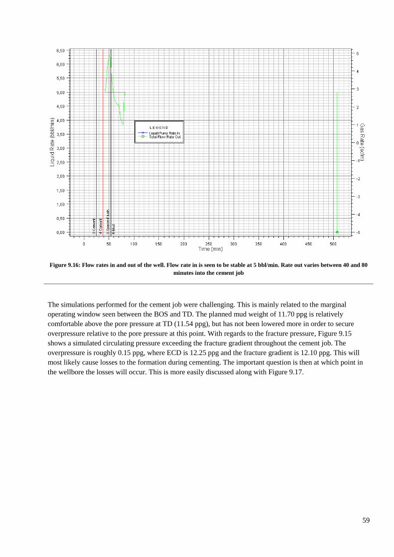
59

Figure 9.16: Flow rates in and out of the well. Flow rate in is seen to be stable at 5 bbl/min. Rate out varies between 40 and 80

minutes into the cement job

The simulations performed for the cement job were challenging. This is mainly related to the marginal

operating window seen between the BOS and TD. The planned mud weight of 11.70 ppg is relatively

comfortable above the pore pressure at TD (11.54 ppg), but has not been lowered more in order to secure

overpressure relative to the pore pressure at this point. With regards to the fracture pressure, Figure 9.15

shows a simulated circulating pressure exceeding the fracture gradient throughout the cement job. The

overpressure is roughly 0.15 ppg, where ECD is 12.25 ppg and the fracture gradient is 12.10 ppg. This will

most likely cause losses to the formation during cementing. The important question is then at which point in

the wellbore the losses will occur. This is more easily discussed along with Figure 9.17.

60

Figure 9.17: ECD and ESD profile seen throughout the well

The ECD is seen to exceed the fracture gradient from BOS to approximately 19 500 ft. The top of cement is

planned at 21 200 ft, 1 700 ft further down compared to the loss zone. This means that the cement

theoretically will be placed at the desired interval, whilst losses or total loss will be experienced at surface.

Here one could take several mitigating actions:

Lower mud weight prior to running casing

Lower mud weight after casing is run

Spot Lost Circulation Material, LCM, pill over potential loss zone in front of or during cement job

The decision on whether to go for 11.70 ppg mud or one of the alternatives above is not clear. As discussed in

Chapter 7, this will depend on several factors. If Well 1 were to be drilled in GoM, this scenario would most

likely not be accepted. A general accepted norm in GoM, is to drill the well with a planned safety margin of

0.5 ppg. On the other hand, this reduction would imply a 0.06 ppg safety margin to the pore pressure.

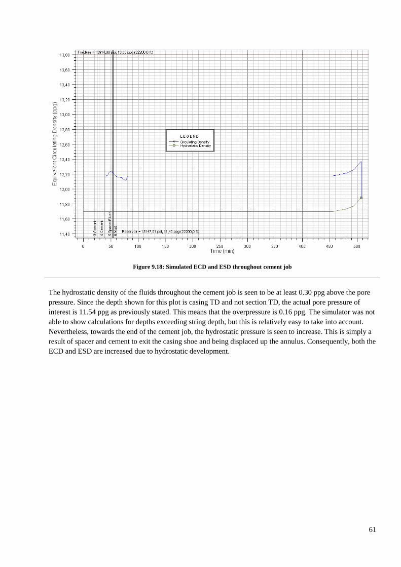
61

Figure 9.18: Simulated ECD and ESD throughout cement job

The hydrostatic density of the fluids throughout the cement job is seen to be at least 0.30 ppg above the pore

pressure. Since the depth shown for this plot is casing TD and not section TD, the actual pore pressure of

interest is 11.54 ppg as previously stated. This means that the overpressure is 0.16 ppg. The simulator was not

able to show calculations for depths exceeding string depth, but this is relatively easy to take into account.

Nevertheless, towards the end of the cement job, the hydrostatic pressure is seen to increase. This is simply a

result of spacer and cement to exit the casing shoe and being displaced up the annulus. Consequently, both the

ECD and ESD are increased due to hydrostatic development.

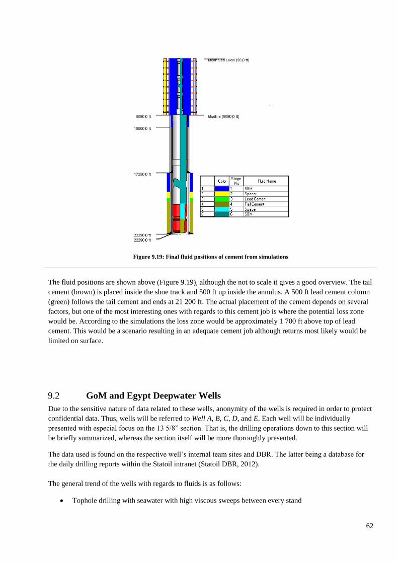
62

Figure 9.19: Final fluid positions of cement from simulations

The fluid positions are shown above (Figure 9.19), although the not to scale it gives a good overview. The tail

cement (brown) is placed inside the shoe track and 500 ft up inside the annulus. A 500 ft lead cement column

(green) follows the tail cement and ends at 21 200 ft. The actual placement of the cement depends on several

factors, but one of the most interesting ones with regards to this cement job is where the potential loss zone

would be. According to the simulations the loss zone would be approximately 1 700 ft above top of lead

cement. This would be a scenario resulting in an adequate cement job although returns most likely would be

limited on surface.

GoM and Egypt Deepwater Wells 9.2

Due to the sensitive nature of data related to these wells, anonymity of the wells is required in order to protect

confidential data. Thus, wells will be referred to Well A, B, C, D, and E. Each well will be individually

presented with especial focus on the 13 5/8” section. That is, the drilling operations down to this section will

be briefly summarized, whereas the section itself will be more thoroughly presented.

The data used is found on the respective well’s internal team sites and DBR. The latter being a database for

the daily drilling reports within the Statoil intranet (Statoil DBR, 2012).

The general trend of the wells with regards to fluids is as follows:

Tophole drilling with seawater with high viscous sweeps between every stand

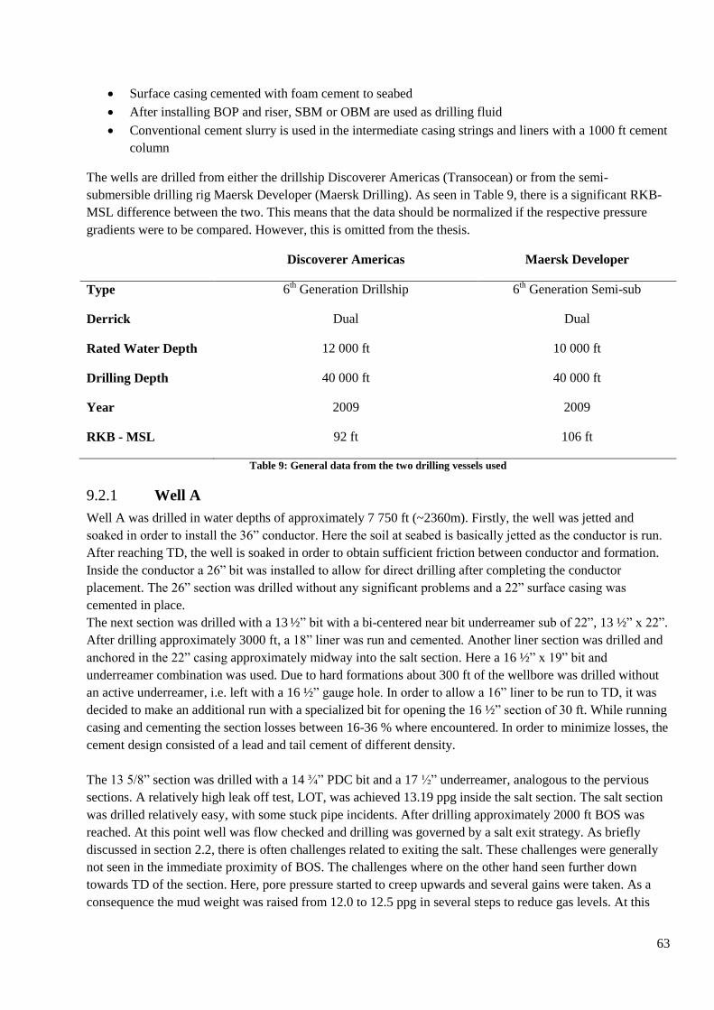
63

Surface casing cemented with foam cement to seabed

After installing BOP and riser, SBM or OBM are used as drilling fluid

Conventional cement slurry is used in the intermediate casing strings and liners with a 1000 ft cement

column

The wells are drilled from either the drillship Discoverer Americas (Transocean) or from the semi-

submersible drilling rig Maersk Developer (Maersk Drilling). As seen in Table 9, there is a significant RKB-

MSL difference between the two. This means that the data should be normalized if the respective pressure

gradients were to be compared. However, this is omitted from the thesis.

Discoverer Americas Maersk Developer

Type

Derrick

6th Generation Drillship

Dual

6th Generation Semi-sub

Dual

Rated Water Depth 12 000 ft 10 000 ft

Drilling Depth 40 000 ft 40 000 ft

Year 2009 2009

RKB - MSL 92 ft 106 ft

Table 9: General data from the two drilling vessels used

Well A 9.2.1

Well A was drilled in water depths of approximately 7 750 ft (~2360m). Firstly, the well was jetted and

soaked in order to install the 36” conductor. Here the soil at seabed is basically jetted as the conductor is run.

After reaching TD, the well is soaked in order to obtain sufficient friction between conductor and formation.

Inside the conductor a 26” bit was installed to allow for direct drilling after completing the conductor

placement. The 26” section was drilled without any significant problems and a 22” surface casing was

cemented in place.

The next section was drilled with a 13 ½” bit with a bi-centered near bit underreamer sub of 22”, 13 ½” x 22”.

After drilling approximately 3000 ft, a 18” liner was run and cemented. Another liner section was drilled and

anchored in the 22” casing approximately midway into the salt section. Here a 16 ½” x 19” bit and

underreamer combination was used. Due to hard formations about 300 ft of the wellbore was drilled without

an active underreamer, i.e. left with a 16 ½” gauge hole. In order to allow a 16” liner to be run to TD, it was

decided to make an additional run with a specialized bit for opening the 16 ½” section of 30 ft. While running

casing and cementing the section losses between 16-36 % where encountered. In order to minimize losses, the

cement design consisted of a lead and tail cement of different density.

The 13 5/8” section was drilled with a 14 ¾” PDC bit and a 17 ½” underreamer, analogous to the pervious

sections. A relatively high leak off test, LOT, was achieved 13.19 ppg inside the salt section. The salt section

was drilled relatively easy, with some stuck pipe incidents. After drilling approximately 2000 ft BOS was

reached. At this point well was flow checked and drilling was governed by a salt exit strategy. As briefly

discussed in section 2.2, there is often challenges related to exiting the salt. These challenges were generally

not seen in the immediate proximity of BOS. The challenges where on the other hand seen further down

towards TD of the section. Here, pore pressure started to creep upwards and several gains were taken. As a

consequence the mud weight was raised from 12.0 to 12.5 ppg in several steps to reduce gas levels. At this

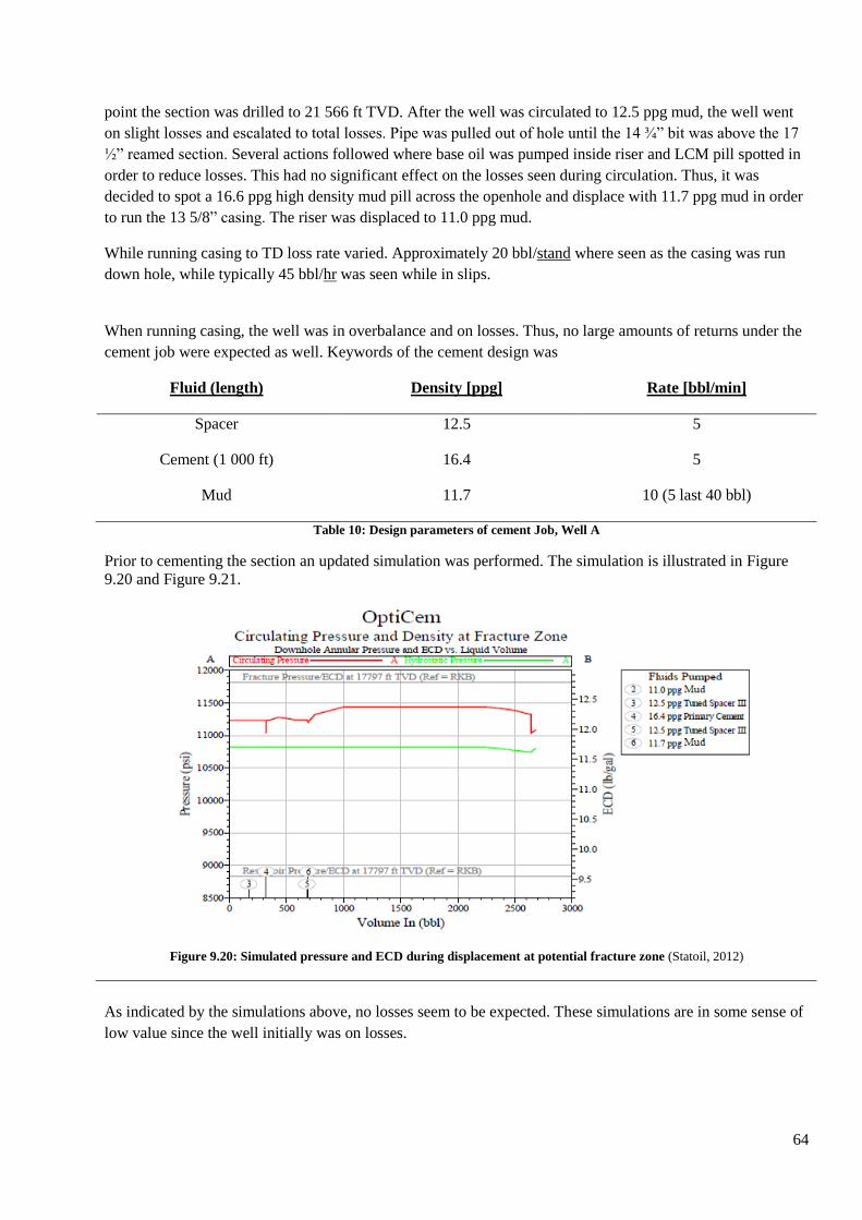
64

point the section was drilled to 21 566 ft TVD. After the well was circulated to 12.5 ppg mud, the well went

on slight losses and escalated to total losses. Pipe was pulled out of hole until the 14 ¾” bit was above the 17

½” reamed section. Several actions followed where base oil was pumped inside riser and LCM pill spotted in

order to reduce losses. This had no significant effect on the losses seen during circulation. Thus, it was

decided to spot a 16.6 ppg high density mud pill across the openhole and displace with 11.7 ppg mud in order

to run the 13 5/8” casing. The riser was displaced to 11.0 ppg mud.

While running casing to TD loss rate varied. Approximately 20 bbl/stand where seen as the casing was run

down hole, while typically 45 bbl/hr was seen while in slips.

When running casing, the well was in overbalance and on losses. Thus, no large amounts of returns under the

cement job were expected as well. Keywords of the cement design was

Fluid (length) Density [ppg] Rate [bbl/min]

Spacer 12.5 5

Cement (1 000 ft) 16.4 5

Mud 11.7 10 (5 last 40 bbl)

Table 10: Design parameters of cement Job, Well A

Prior to cementing the section an updated simulation was performed. The simulation is illustrated in Figure

9.20 and Figure 9.21.

Figure 9.20: Simulated pressure and ECD during displacement at potential fracture zone (Statoil, 2012)

As indicated by the simulations above, no losses seem to be expected. These simulations are in some sense of

low value since the well initially was on losses.

65

Figure 9.21: Simulated pressure and ECD during displacement at potential flow zone (Statoil, 2012)

At 20 257 ft a potential flow zone or reservoir zone is evaluated and significant risk for inflow seem to be

present.

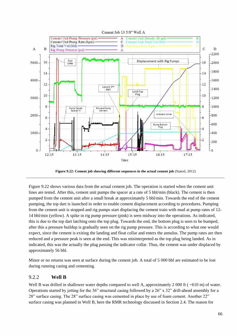
66

Figure 9.22: Cement job showing different sequences in the actual cement job (Statoil, 2012)

Figure 9.22 shows various data from the actual cement job. The operation is started when the cement unit

lines are tested. After this, cement unit pumps the spacer at a rate of 5 bbl/min (black). The cement is then

pumped from the cement unit after a small break at approximately 5 bbl/min. Towards the end of the cement

pumping, the top dart is launched in order to enable cement displacement according to procedures. Pumping

from the cement unit is stopped and rig pumps start displacing the cement train with mud at pump rates of 12-

14 bbl/min (yellow). A spike in rig pump pressure (pink) is seen midway into the operations. As indicated,

this is due to the top dart latching onto the top plug. Towards the end, the bottom plug is seen to be bumped,

after this a pressure buildup is gradually seen on the rig pump pressure. This is according to what one would

expect, since the cement is exiting the landing and float collar and enters the annulus. The pump rates are then

reduced and a pressure peak is seen at the end. This was misinterpreted as the top plug being landed. As in

indicated, this was the actually the plug passing the indicator collar. Thus, the cement was under displaced by

approximately 56 bbl.

Minor or no returns was seen at surface during the cement job. A total of 5 000 bbl are estimated to be lost

during running casing and cementing.

Well B 9.2.2

Well B was drilled in shallower water depths compared to well A, approximately 2 000 ft ( ~610 m) of water.

Operations started by jetting for the 36” structural casing followed by a 26” x 32” drill-ahead assembly for a

28” surface casing. The 28” surface casing was cemented in place by use of foam cement. Another 22”

surface casing was planned in Well B, here the RMR technology discussed in Section 2.4. The reason for

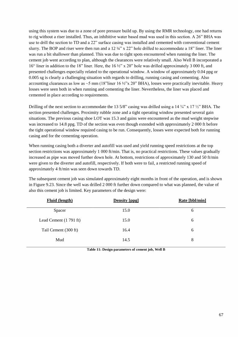
67

using this system was due to a zone of pore pressure build up. By using the RMR technology, one had returns

to rig without a riser installed. Thus, an inhibitive water based mud was used in this section. A 26” BHA was

use to drill the section to TD and a 22” surface casing was installed and cemented with conventional cement

slurry. The BOP and riser were then run and a 12 ¼” x 22” hole drilled to accommodate a 18” liner. The liner

was run a bit shallower than planned. This was due to tight spots encountered when running the liner. The

cement job went according to plan, although the clearances were relatively small. Also Well B incorporated a

16“ liner in addition to the 18” liner. Here, the 16 ½” x 20” hole was drilled approximately 3 000 ft, and

presented challenges especially related to the operational window. A window of approximately 0.04 ppg or

0.005 sg is clearly a challenging situation with regards to drilling, running casing and cementing. Also

accounting clearances as low as ~5 mm (18”liner 16 ½”x 20” BHA), losses were practically inevitable. Heavy

losses were seen both in when running and cementing the liner. Nevertheless, the liner was placed and

cemented in place according to requirements.

Drilling of the next section to accommodate the 13 5/8” casing was drilled using a 14 ¾” x 17 ½” BHA. The

section presented challenges. Proximity rubble zone and a tight operating window presented several gain

situations. The previous casing shoe LOT was 15.3 and gains were encountered as the mud weight stepwise

was increased to 14.8 ppg. TD of the section was even though extended with approximately 2 000 ft before

the tight operational window required casing to be run. Consequently, losses were expected both for running

casing and for the cementing operation.

When running casing both a diverter and autofill was used and yield running speed restrictions at the top

section restrictions was approximately 1 000 ft/min. That is, no practical restrictions. These values gradually

increased as pipe was moved further down hole. At bottom, restrictions of approximately 130 and 50 ft/min

were given to the diverter and autofill, respectively. If both were to fail, a restricted running speed of

approximately 4 ft/min was seen down towards TD.

The subsequent cement job was simulated approximately eight months in front of the operation, and is shown

in Figure 9.23. Since the well was drilled 2 000 ft further down compared to what was planned, the value of

also this cement job is limited. Key parameters of the design were:

Fluid (length) Density [ppg] Rate [bbl/min]

Spacer 15.0 6

Lead Cement (1 791 ft) 15.0 6

Tail Cement (300 ft) 16.4 6

Mud 14.5 8

Table 11: Design parameters of cement job, Well B

68

Figure 9.23: Simulated pressure and ECD during displacement at potential fracture zone (Statoil, 2012)

As seen in this figure, the circulating pressure is high and close to the fracture pressure. After circulating 1

500 bbls the fracture pressure is exceeded, most likely leading to losses. The increase in ECD and ESD is the

cement being placed over the section.

The cement job record from the rig was acquired. The data is shown in Figure 9.24.

Figure 9.24: Real time data from cement job, Well B (Statoil, 2012)

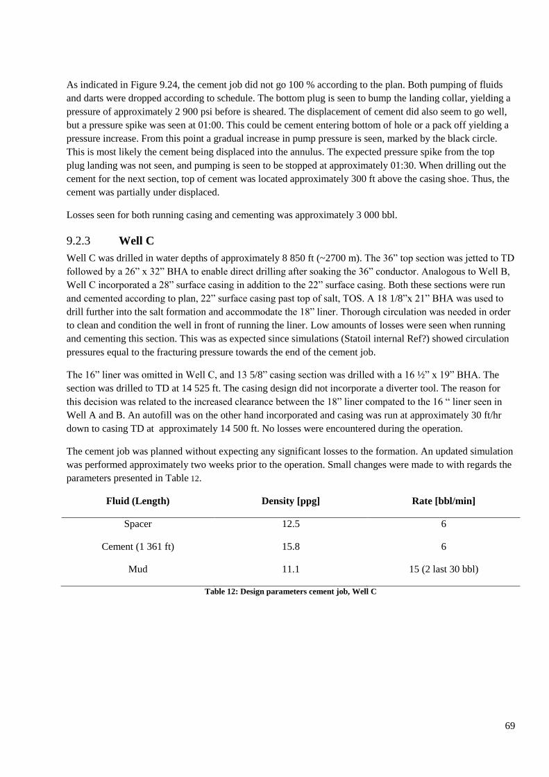
69

As indicated in Figure 9.24, the cement job did not go 100 % according to the plan. Both pumping of fluids

and darts were dropped according to schedule. The bottom plug is seen to bump the landing collar, yielding a

pressure of approximately 2 900 psi before is sheared. The displacement of cement did also seem to go well,

but a pressure spike was seen at 01:00. This could be cement entering bottom of hole or a pack off yielding a

pressure increase. From this point a gradual increase in pump pressure is seen, marked by the black circle.

This is most likely the cement being displaced into the annulus. The expected pressure spike from the top

plug landing was not seen, and pumping is seen to be stopped at approximately 01:30. When drilling out the

cement for the next section, top of cement was located approximately 300 ft above the casing shoe. Thus, the

cement was partially under displaced.

Losses seen for both running casing and cementing was approximately 3 000 bbl.

Well C 9.2.3

Well C was drilled in water depths of approximately 8 850 ft (~2700 m). The 36” top section was jetted to TD

followed by a 26” x 32” BHA to enable direct drilling after soaking the 36” conductor. Analogous to Well B,

Well C incorporated a 28” surface casing in addition to the 22” surface casing. Both these sections were run

and cemented according to plan, 22” surface casing past top of salt, TOS. A 18 1/8”x 21” BHA was used to

drill further into the salt formation and accommodate the 18” liner. Thorough circulation was needed in order

to clean and condition the well in front of running the liner. Low amounts of losses were seen when running

and cementing this section. This was as expected since simulations (Statoil internal Ref?) showed circulation

pressures equal to the fracturing pressure towards the end of the cement job.

The 16” liner was omitted in Well C, and 13 5/8” casing section was drilled with a 16 ½” x 19” BHA. The

section was drilled to TD at 14 525 ft. The casing design did not incorporate a diverter tool. The reason for

this decision was related to the increased clearance between the 18” liner compated to the 16 “ liner seen in

Well A and B. An autofill was on the other hand incorporated and casing was run at approximately 30 ft/hr

down to casing TD at approximately 14 500 ft. No losses were encountered during the operation.

The cement job was planned without expecting any significant losses to the formation. An updated simulation

was performed approximately two weeks prior to the operation. Small changes were made to with regards the

parameters presented in Table 12.

Fluid (Length) Density [ppg] Rate [bbl/min]

Spacer 12.5 6

Cement (1 361 ft) 15.8 6

Mud 11.1 15 (2 last 30 bbl)

Table 12: Design parameters cement job, Well C

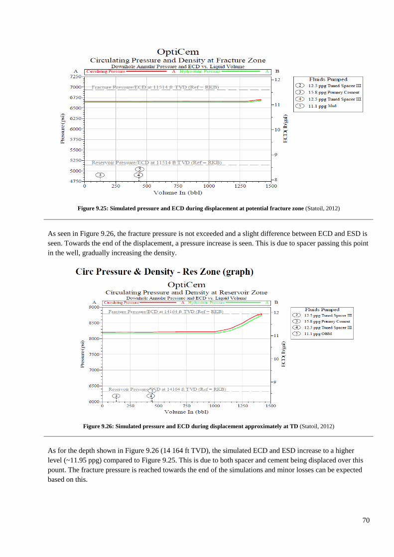
70

Figure 9.25: Simulated pressure and ECD during displacement at potential fracture zone (Statoil, 2012)

As seen in Figure 9.26, the fracture pressure is not exceeded and a slight difference between ECD and ESD is

seen. Towards the end of the displacement, a pressure increase is seen. This is due to spacer passing this point

in the well, gradually increasing the density.

Figure 9.26: Simulated pressure and ECD during displacement approximately at TD (Statoil, 2012)

As for the depth shown in Figure 9.26 (14 164 ft TVD), the simulated ECD and ESD increase to a higher

level (~11.95 ppg) compared to Figure 9.25. This is due to both spacer and cement being displaced over this

pount. The fracture pressure is reached towards the end of the simulations and minor losses can be expected

based on this.

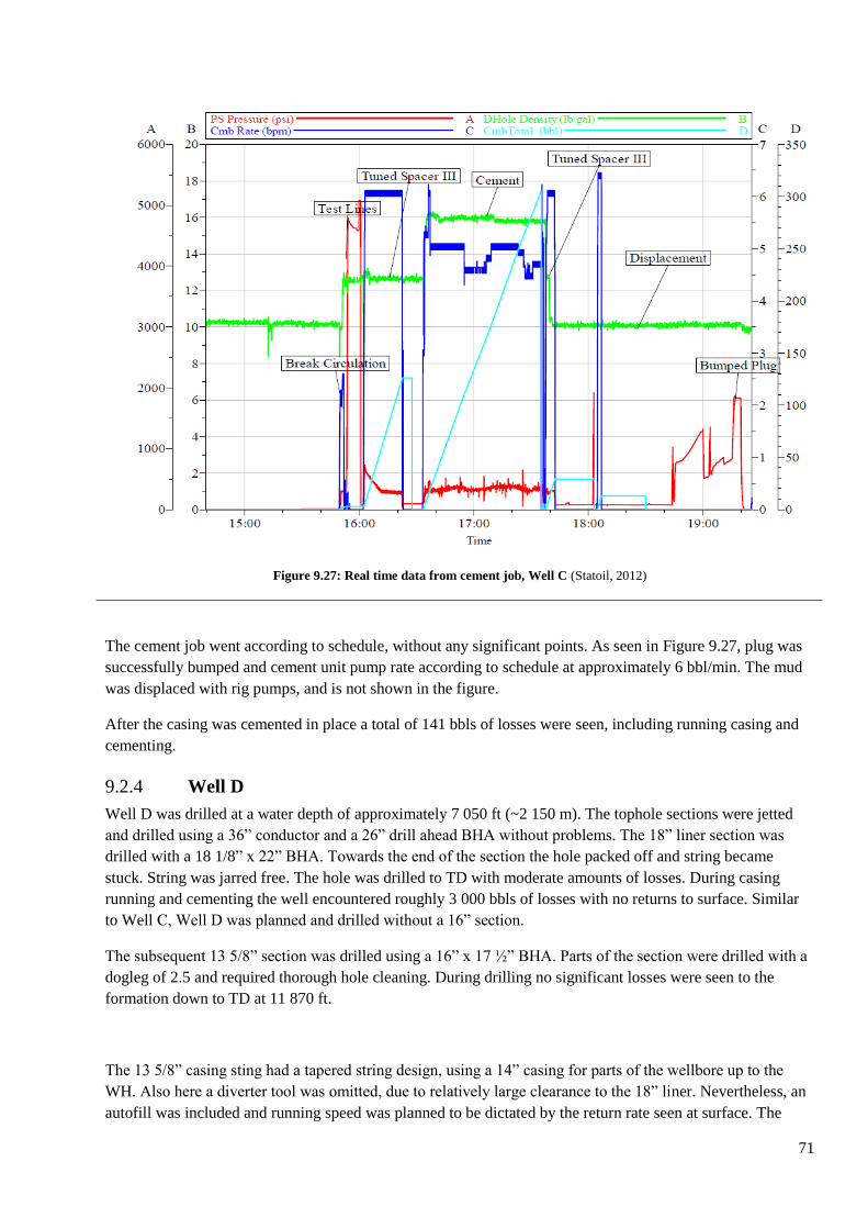
71

Figure 9.27: Real time data from cement job, Well C (Statoil, 2012)

The cement job went according to schedule, without any significant points. As seen in Figure 9.27, plug was

successfully bumped and cement unit pump rate according to schedule at approximately 6 bbl/min. The mud

was displaced with rig pumps, and is not shown in the figure.

After the casing was cemented in place a total of 141 bbls of losses were seen, including running casing and

cementing.

Well D 9.2.4

Well D was drilled at a water depth of approximately 7 050 ft (~2 150 m). The tophole sections were jetted

and drilled using a 36” conductor and a 26” drill ahead BHA without problems. The 18” liner section was

drilled with a 18 1/8” x 22” BHA. Towards the end of the section the hole packed off and string became

stuck. String was jarred free. The hole was drilled to TD with moderate amounts of losses. During casing

running and cementing the well encountered roughly 3 000 bbls of losses with no returns to surface. Similar

to Well C, Well D was planned and drilled without a 16” section.

The subsequent 13 5/8” section was drilled using a 16” x 17 ½” BHA. Parts of the section were drilled with a

dogleg of 2.5 and required thorough hole cleaning. During drilling no significant losses were seen to the

formation down to TD at 11 870 ft.

The 13 5/8” casing sting had a tapered string design, using a 14” casing for parts of the wellbore up to the

WH. Also here a diverter tool was omitted, due to relatively large clearance to the 18” liner. Nevertheless, an

autofill was included and running speed was planned to be dictated by the return rate seen at surface. The

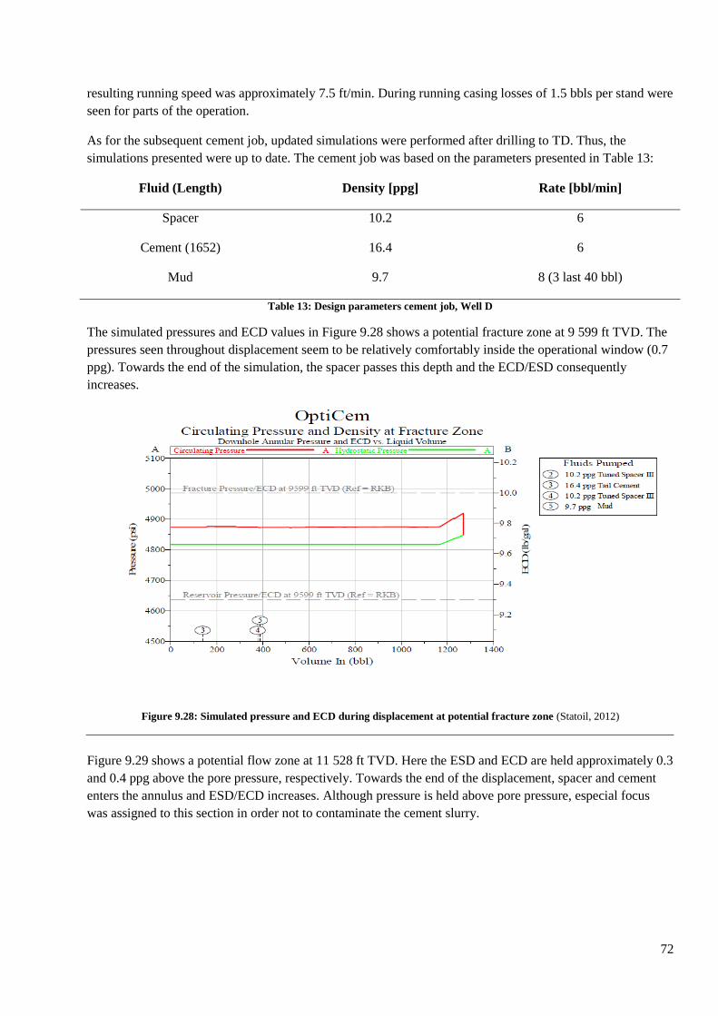
72

resulting running speed was approximately 7.5 ft/min. During running casing losses of 1.5 bbls per stand were

seen for parts of the operation.

As for the subsequent cement job, updated simulations were performed after drilling to TD. Thus, the

simulations presented were up to date. The cement job was based on the parameters presented in Table 13:

Fluid (Length) Density [ppg] Rate [bbl/min]

Spacer 10.2 6

Cement (1652) 16.4 6

Mud 9.7 8 (3 last 40 bbl)

Table 13: Design parameters cement job, Well D

The simulated pressures and ECD values in Figure 9.28 shows a potential fracture zone at 9 599 ft TVD. The

pressures seen throughout displacement seem to be relatively comfortably inside the operational window (0.7

ppg). Towards the end of the simulation, the spacer passes this depth and the ECD/ESD consequently

increases.

Figure 9.28: Simulated pressure and ECD during displacement at potential fracture zone (Statoil, 2012)

Figure 9.29 shows a potential flow zone at 11 528 ft TVD. Here the ESD and ECD are held approximately 0.3

and 0.4 ppg above the pore pressure, respectively. Towards the end of the displacement, spacer and cement

enters the annulus and ESD/ECD increases. Although pressure is held above pore pressure, especial focus

was assigned to this section in order not to contaminate the cement slurry.

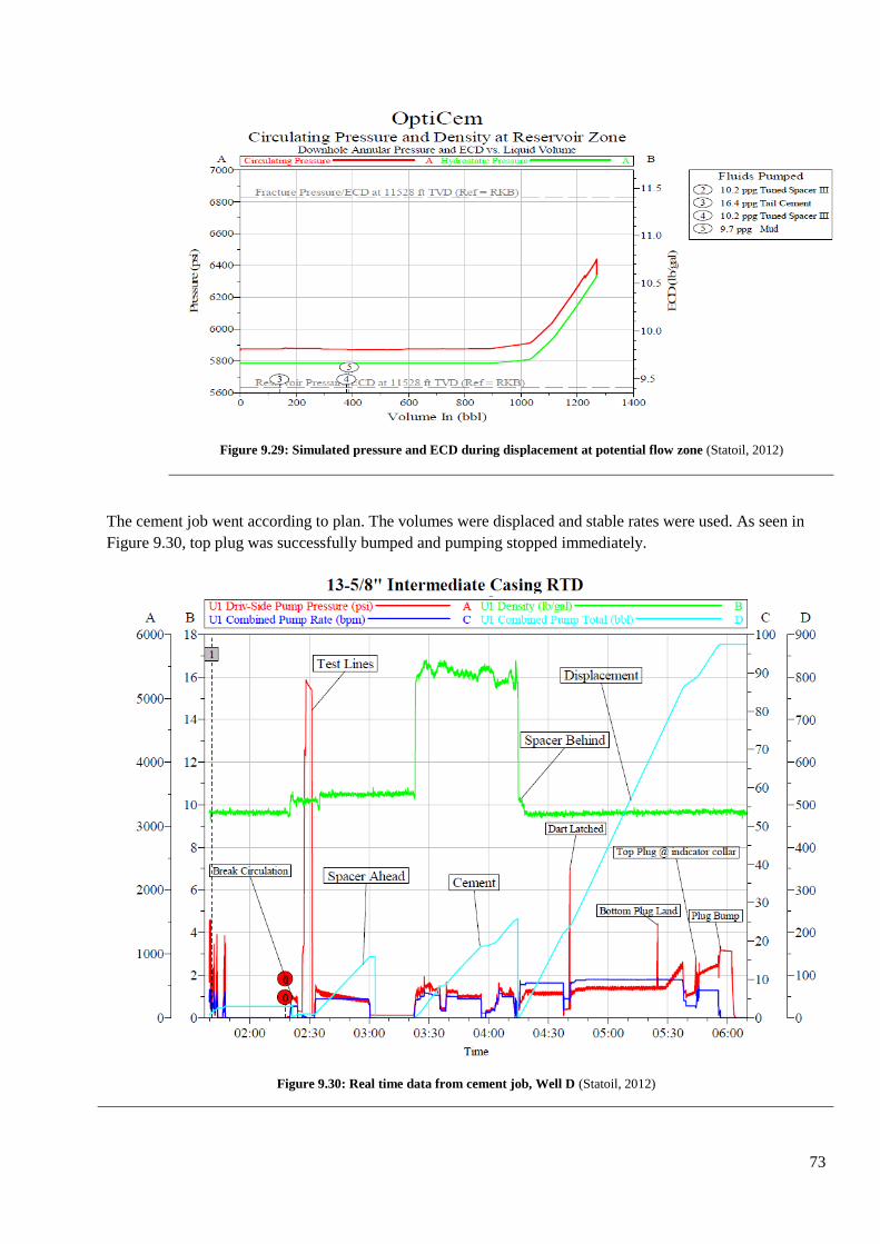
73

Figure 9.29: Simulated pressure and ECD during displacement at potential flow zone (Statoil, 2012)

The cement job went according to plan. The volumes were displaced and stable rates were used. As seen in

Figure 9.30, top plug was successfully bumped and pumping stopped immediately.

Figure 9.30: Real time data from cement job, Well D (Statoil, 2012)

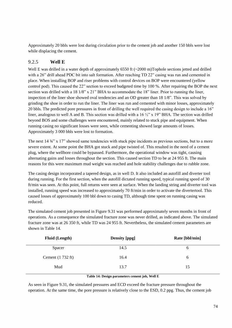
74

Approximately 20 bbls were lost during circulation prior to the cement job and another 150 bbls were lost

while displacing the cement.

Well E 9.2.5

Well E was drilled in a water depth of approximately 6550 ft (~2000 m)Tophole sections jetted and drilled

with a 26” drill ahead PDC bit into salt formation. After reaching TD 22” casing was run and cemented in

place. When installing BOP and riser problems with control devices on BOP were encountered (yellow

control pod). This caused the 22” section to exceed budgeted time by 100 %. After repairing the BOP the next

section was drilled with a 18 1/8” x 21” BHA to accommodate the 18” liner. Prior to running the liner,

inspection of the liner shoe showed oval tendencies and an OD greater than 18 1/8”. This was solved by

grinding the shoe in order to run the liner. The liner was run and cemented with minor losses, approximately

20 bbls. The predicted pore pressures in front of drilling the well required the casing design to include a 16”

liner, analogous to well A and B. This section was drilled with a 16 ½” x 19” BHA. The section was drilled

beyond BOS and some challenges were encountered, mainly related to stuck pipe and equipment. When

running casing no significant losses were seen, while cementing showed large amounts of losses.

Approximately 3 000 bbls were lost to formation.

The next 14 ¾” x 17” showed same tendencies with stuck pipe incidents as previous sections, but to a more

severe extent. At some point the BHA got stuck and pipe twisted of. This resulted in the need of a cement

plug, where the wellbore could be bypassed. Furthermore, the operational window was tight, causing

alternating gains and losses throughout the section. This caused section TD to be at 24 955 ft. The main

reasons for this were maximum mud weight was reached and hole stability challenges due to rubble zone.

The casing design incorporated a tapered design, as in well D. It also included an autofill and diverter tool

during running. For the first section, when the autofill dictated running speed, typical running speed of 30

ft/min was seen. At this point, full returns were seen at surface. When the landing string and diverter tool was

installed, running speed was increased to approximately 70 ft/min in order to activate the divertertool. This

caused losses of approximately 100 bbl down to casing TD, although time spent on running casing was

reduced.

The simulated cement job presented in Figure 9.31 was performed approximately seven months in front of

operations. As a consequence the simulated fracture zone was never drilled, as indicated above. The simulated

fracture zone was at 26 350 ft, while TD was 24 955 ft. Nevertheless, the simulated cement parameters are

shown in Table 14.

Fluid (Length) Density [ppg] Rate [bbl/min]

Spacer 14.5 6

Cement (1 732 ft) 16.4 6

Mud 13.7 15

Table 14: Design parameters cement job, Well E

As seen in Figure 9.31, the simulated pressures and ECD exceed the fracture pressure throughout the

operation. At the same time, the pore pressure is relatively close to the ESD, 0.2 ppg. Thus, the cement job

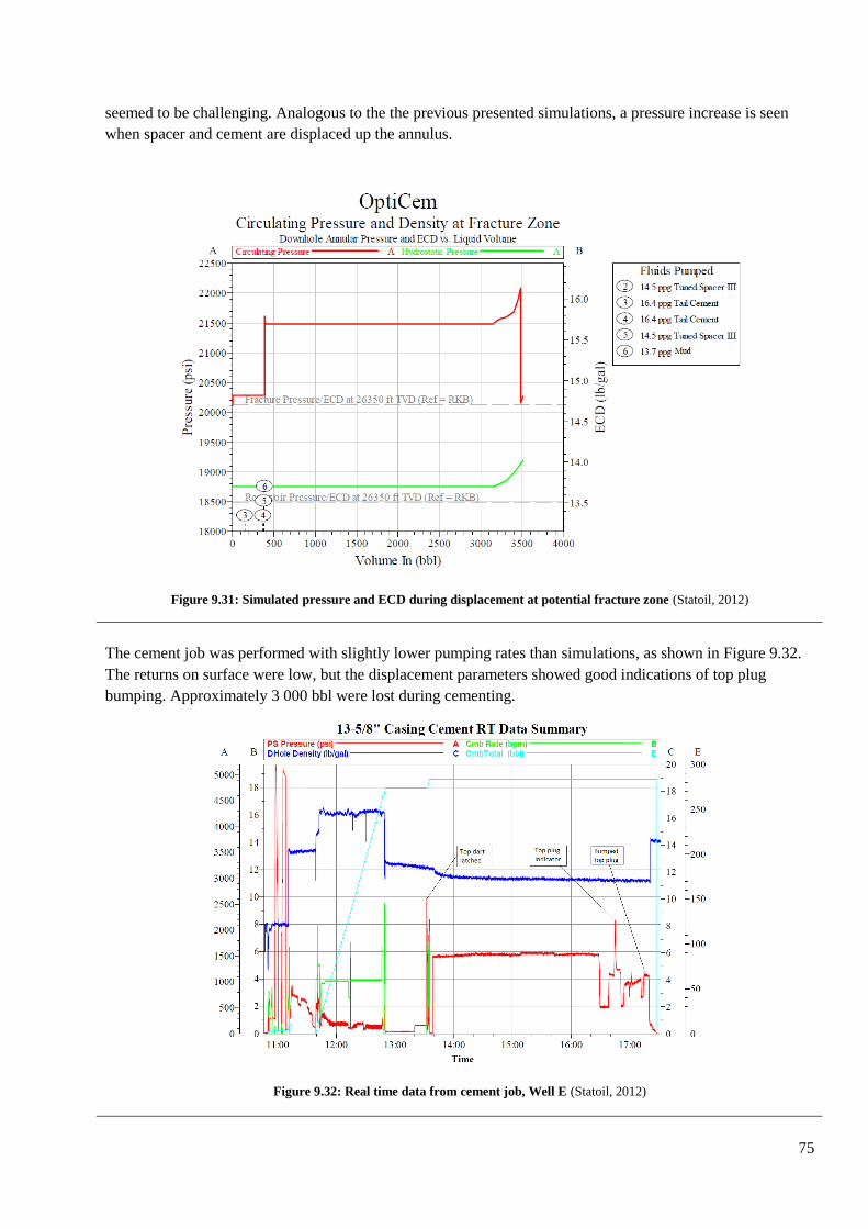
75

seemed to be challenging. Analogous to the the previous presented simulations, a pressure increase is seen

when spacer and cement are displaced up the annulus.

Figure 9.31: Simulated pressure and ECD during displacement at potential fracture zone (Statoil, 2012)

The cement job was performed with slightly lower pumping rates than simulations, as shown in Figure 9.32.

The returns on surface were low, but the displacement parameters showed good indications of top plug

bumping. Approximately 3 000 bbl were lost during cementing.

Figure 9.32: Real time data from cement job, Well E (Statoil, 2012)

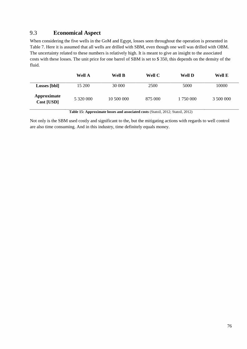
76

Economical Aspect 9.3

When considering the five wells in the GoM and Egypt, losses seen throughout the operation is presented in

Table 7. Here it is assumed that all wells are drilled with SBM, even though one well was drilled with OBM.

The uncertainty related to these numbers is relatively high. It is meant to give an insight to the associated

costs with these losses. The unit price for one barrel of SBM is set to $ 350, this depends on the density of the

fluid.

Well A Well B Well C Well D Well E

Losses [bbl] 15 200 30 000 2500 5000 10000

Approximate

Cost [USD] 5 320 000 10 500 000 875 000 1 750 000 3 500 000

Table 15: Approximate losses and associated costs (Statoil, 2012; Statoil, 2012)

Not only is the SBM used costly and significant to the, but the mitigating actions with regards to well control

are also time consuming. And in this industry, time definitely equals money.

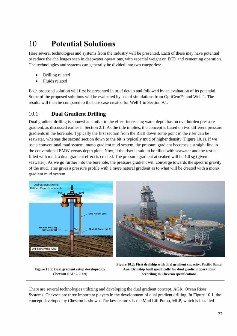
77

Potential Solutions 10Here several technologies and systems from the industry will be presented. Each of these may have potential

to reduce the challenges seen in deepwater operations, with especial weight on ECD and cementing operation.

The technologies and systems can generally be divided into two categories:

Drilling related

Fluids related

Each proposed solution will first be presented in brief detain and followed by an evaluation of its potential.

Some of the proposed solutions will be evaluated by use of simulations from OptiCem™ and Well 1. The

results will then be compared to the base case created for Well 1 in Section 9.1.

Dual Gradient Drilling 10.1

Dual gradient drilling is somewhat similar to the effect increasing water depth has on overburden pressure

gradient, as discussed earlier in Section 2.1. As the title implies, the concept is based on two different pressure

gradients in the borehole. Typically the first section from the RKB down some point in the riser can be

seawater, whereas the second section down to the bit is typically mud of higher density (Figure 10.1). If we

use a conventional mud system, mono gradient mud system, the pressure gradient becomes a straight line in

the conventional EMW versus depth plots. Now, if the riser is said to be filled with seawater and the rest is

filled with mud, a dual gradient effect is created. The pressure gradient at seabed will be 1.0 sg (given

seawater). As we go further into the borehole, the pressure gradient will converge towards the specific gravity

of the mud. This gives a pressure profile with a more natural gradient as to what will be created with a mono

gradient mud system.

Figure 10.1: Dual gradient setup developed by

Chevron (IADC, 2009)

Figure 10.2: First drillship with dual gradient capacity, Pacific Santa

Ana. Drillship built specifically for dual gradient operations

according to Chevron specifications

There are several technologies utilizing and developing the dual gradient concept. AGR, Ocean Riser

Systems, Chevron are three important players in the development of dual gradient drilling. In Figure 10.1, the

concept developed by Chevron is shown. The key features is the Mud Lift Pump, MLP, which is installed

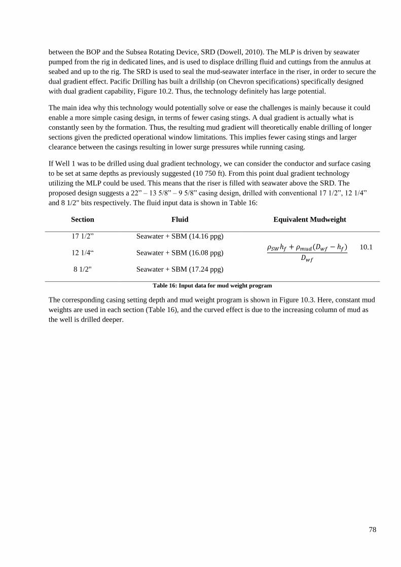
78

between the BOP and the Subsea Rotating Device, SRD (Dowell, 2010). The MLP is driven by seawater

pumped from the rig in dedicated lines, and is used to displace drilling fluid and cuttings from the annulus at

seabed and up to the rig. The SRD is used to seal the mud-seawater interface in the riser, in order to secure the

dual gradient effect. Pacific Drilling has built a drillship (on Chevron specifications) specifically designed

with dual gradient capability, Figure 10.2. Thus, the technology definitely has large potential.

The main idea why this technology would potentially solve or ease the challenges is mainly because it could

enable a more simple casing design, in terms of fewer casing stings. A dual gradient is actually what is

constantly seen by the formation. Thus, the resulting mud gradient will theoretically enable drilling of longer

sections given the predicted operational window limitations. This implies fewer casing stings and larger

clearance between the casings resulting in lower surge pressures while running casing.

If Well 1 was to be drilled using dual gradient technology, we can consider the conductor and surface casing

to be set at same depths as previously suggested (10 750 ft). From this point dual gradient technology

utilizing the MLP could be used. This means that the riser is filled with seawater above the SRD. The

proposed design suggests a 22” – 13 5/8” – 9 5/8” casing design, drilled with conventional 17 1/2”, 12 1/4”

and 8 1/2" bits respectively. The fluid input data is shown in Table 16:

Section Fluid Equivalent Mudweight

17 1/2” Seawater + SBM (14.16 ppg)

10.1

12 1/4“ Seawater + SBM (16.08 ppg)

8 1/2" Seawater + SBM (17.24 ppg)

Table 16: Input data for mud weight program

The corresponding casing setting depth and mud weight program is shown in Figure 10.3. Here, constant mud

weights are used in each section (Table 16), and the curved effect is due to the increasing column of mud as

the well is drilled deeper.

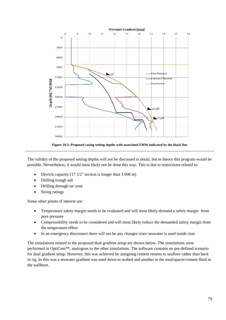
79

Figure 10.3: Proposed casing setting depths with associated EMW indicated by the black line

The validity of the proposed setting depths will not be discussed in detail, but in theory this program would be

possible. Nevertheless, it would most likely not be done this way. This is due to restrictions related to:

Derrick capacity (17 1/2" section is longer than 3 000 m)

Drilling trough salt

Drilling through tar zone

String ratings

Some other points of interest are:

Temperature safety margin needs to be evaluated and will most likely demand a safety margin from

pore pressure

Compressibility needs to be considered and will most likely reduce the demanded safety margin from

the temperature effect

In an emergency disconnect there will not be any changes since seawater is used inside riser

The simulations related to the proposed dual gradient setup are shown below. The simulations were

performed in OptiCem™, analogous to the other simulations. The software contains no pre-defined scenario

for dual gradient setup. However, this was achieved by assigning cement returns to seafloor rather than back

to rig. In this was a seawater gradient was used down to seabed and another in the mud/spacer/cement fluid in

the wellbore.

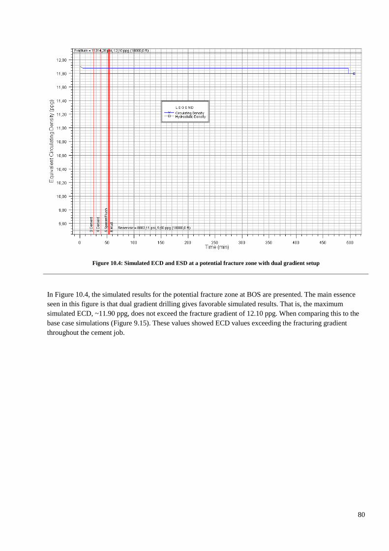
80

Figure 10.4: Simulated ECD and ESD at a potential fracture zone with dual gradient setup

In Figure 10.4, the simulated results for the potential fracture zone at BOS are presented. The main essence

seen in this figure is that dual gradient drilling gives favorable simulated results. That is, the maximum

simulated ECD, ~11.90 ppg, does not exceed the fracture gradient of 12.10 ppg. When comparing this to the

base case simulations (Figure 9.15). These values showed ECD values exceeding the fracturing gradient

throughout the cement job.

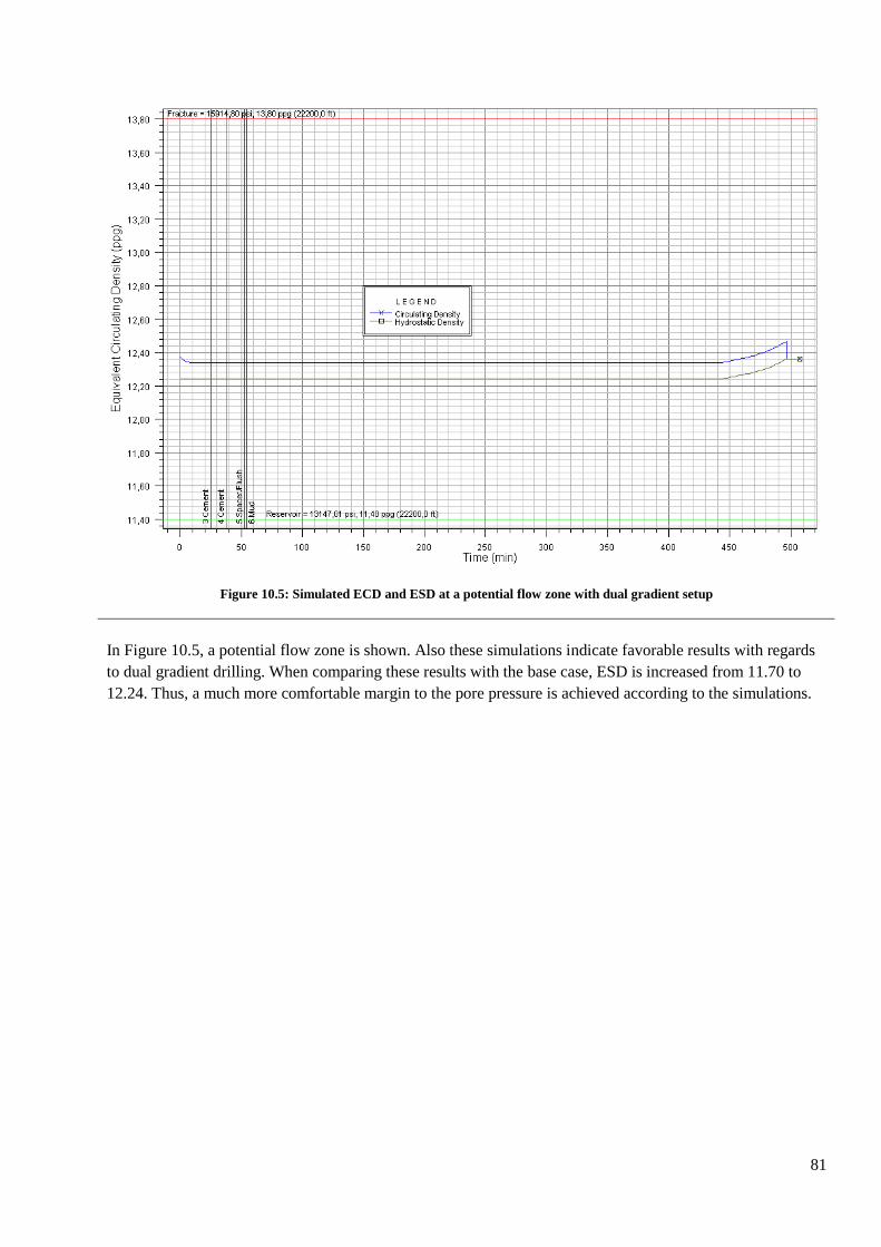
81

Figure 10.5: Simulated ECD and ESD at a potential flow zone with dual gradient setup

In Figure 10.5, a potential flow zone is shown. Also these simulations indicate favorable results with regards

to dual gradient drilling. When comparing these results with the base case, ESD is increased from 11.70 to

12.24. Thus, a much more comfortable margin to the pore pressure is achieved according to the simulations.

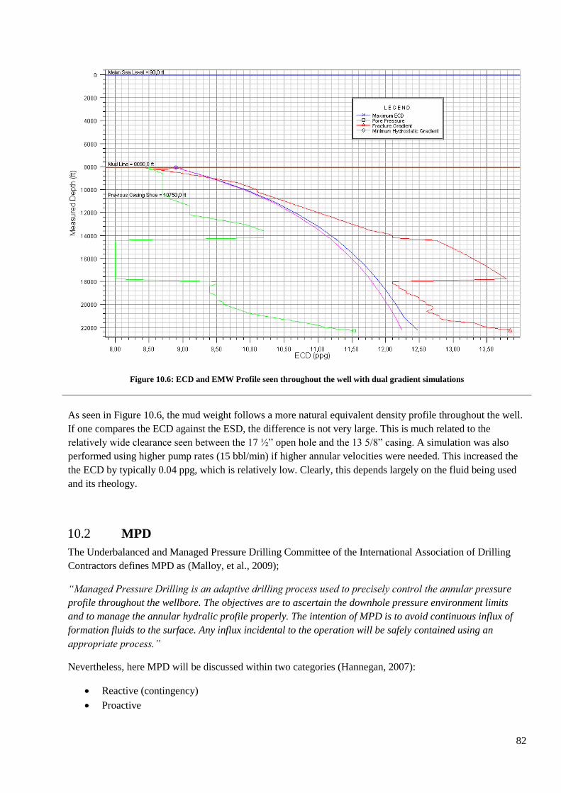
82

Figure 10.6: ECD and EMW Profile seen throughout the well with dual gradient simulations

As seen in Figure 10.6, the mud weight follows a more natural equivalent density profile throughout the well.

If one compares the ECD against the ESD, the difference is not very large. This is much related to the

relatively wide clearance seen between the 17 ½” open hole and the 13 5/8” casing. A simulation was also

performed using higher pump rates (15 bbl/min) if higher annular velocities were needed. This increased the

the ECD by typically 0.04 ppg, which is relatively low. Clearly, this depends largely on the fluid being used

and its rheology.

MPD 10.2

The Underbalanced and Managed Pressure Drilling Committee of the International Association of Drilling

Contractors defines MPD as (Malloy, et al., 2009);

“Managed Pressure Drilling is an adaptive drilling process used to precisely control the annular pressure

profile throughout the wellbore. The objectives are to ascertain the downhole pressure environment limits

and to manage the annular hydralic profile properly. The intention of MPD is to avoid continuous influx of

formation fluids to the surface. Any influx incidental to the operation will be safely contained using an

appropriate process.”

Nevertheless, here MPD will be discussed within two categories (Hannegan, 2007):

Reactive (contingency)

Proactive

83

The difference is basically whether MPD is planned to be used as a contingency solution to a problem

(reactive) or used from the beginning of the drilling operation.

Some of the existing technologies are annular back pressure pump systems (Weatherford, Halliburton,

Schlumberger) and Continous Circulations System, CCS, (NOV). The key to the Annular back pressure pump

system (Figure 10.7) is the Rotating Control Device, RCD (Figure 10.8), typically located above the BOP.

The RCD functions as a sealing mechanism and diverts flow from the annulus into a choke manifold. By

regulating the choke, the bottom hole pressure is controlled. During a connection, an annular back pressure

pump is activated and gradually ramped up as the rig pumps are ramped down. In this way there is always

flow over the choke, either form rig pumps or back pressure pump. Thus, the bottom hole pressure can

theoretically be held constant.

Figure 10.7:Setup of a MPD system (Breyholtz, et al., 2010) Figure 10.8:RCD from Weatherford

If one compares the presented MPD system with the dual gradient system above, the effect can be compared.

The only difference is that the dual gradient created in the MPD system will consist of a pressure gradient

caused from the choke and another gradient filling the string and annulus. Thus, the EMW as one drill further

into the hole is a reversed curve compared to dual gradient EMW. This is shown in Figure 10.9.

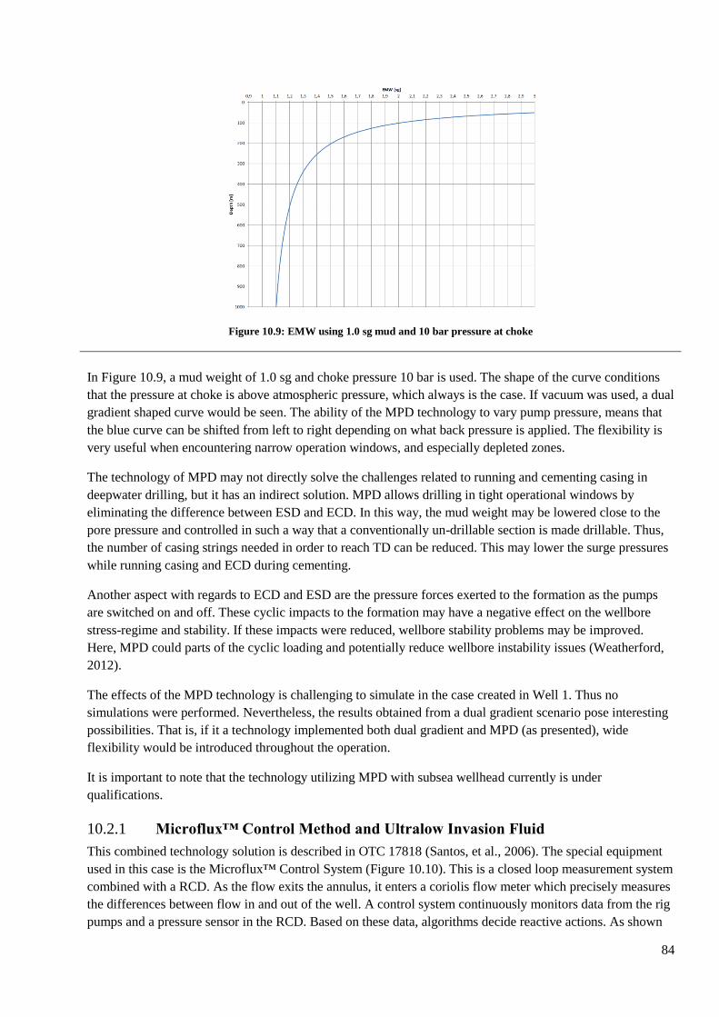
84

Figure 10.9: EMW using 1.0 sg mud and 10 bar pressure at choke

In Figure 10.9, a mud weight of 1.0 sg and choke pressure 10 bar is used. The shape of the curve conditions

that the pressure at choke is above atmospheric pressure, which always is the case. If vacuum was used, a dual

gradient shaped curve would be seen. The ability of the MPD technology to vary pump pressure, means that

the blue curve can be shifted from left to right depending on what back pressure is applied. The flexibility is

very useful when encountering narrow operation windows, and especially depleted zones.

The technology of MPD may not directly solve the challenges related to running and cementing casing in

deepwater drilling, but it has an indirect solution. MPD allows drilling in tight operational windows by

eliminating the difference between ESD and ECD. In this way, the mud weight may be lowered close to the

pore pressure and controlled in such a way that a conventionally un-drillable section is made drillable. Thus,

the number of casing strings needed in order to reach TD can be reduced. This may lower the surge pressures

while running casing and ECD during cementing.

Another aspect with regards to ECD and ESD are the pressure forces exerted to the formation as the pumps

are switched on and off. These cyclic impacts to the formation may have a negative effect on the wellbore

stress-regime and stability. If these impacts were reduced, wellbore stability problems may be improved.

Here, MPD could parts of the cyclic loading and potentially reduce wellbore instability issues (Weatherford,

2012).

The effects of the MPD technology is challenging to simulate in the case created in Well 1. Thus no

simulations were performed. Nevertheless, the results obtained from a dual gradient scenario pose interesting

possibilities. That is, if it a technology implemented both dual gradient and MPD (as presented), wide

flexibility would be introduced throughout the operation.

It is important to note that the technology utilizing MPD with subsea wellhead currently is under

qualifications.

Microflux™ Control Method and Ultralow Invasion Fluid 10.2.1

This combined technology solution is described in OTC 17818 (Santos, et al., 2006). The special equipment

used in this case is the Microflux™ Control System (Figure 10.10). This is a closed loop measurement system

combined with a RCD. As the flow exits the annulus, it enters a coriolis flow meter which precisely measures

the differences between flow in and out of the well. A control system continuously monitors data from the rig

pumps and a pressure sensor in the RCD. Based on these data, algorithms decide reactive actions. As shown

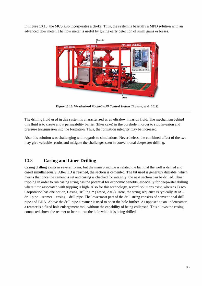
85

in Figure 10.10, the MCS also incorporates a choke. Thus, the system is basically a MPD solution with an

advanced flow meter. The flow meter is useful by giving early detection of small gains or losses.

Figure 10.10: Weatherford Mictroflux™ Control System (Grayson, et al., 2011)

The drilling fluid used in this system is characterized as an ultralow invasion fluid. The mechanism behind

this fluid is to create a low permeability barrier (filter cake) in the borehole in order to stop invasion and

pressure transmission into the formation. Thus, the formation integrity may be increased.

Also this solution was challenging with regards to simulations. Nevertheless, the combined effect of the two

may give valuable results and mitigate the challenges seen in conventional deepwater drilling.

Casing and Liner Drilling 10.3

Casing drilling exists in several forms, but the main principle is related the fact that the well is drilled and

cased simultaneously. After TD is reached, the section is cemented. The bit used is generally drillable, which

means that once the cement is set and casing is checked for integrity, the next section can be drilled. Thus,

tripping in order to run casing string has the potential for economic benefits, especially for deepwater drilling

where time associated with tripping is high. Also for this technology, several solutions exist, whereas Tesco

Corporation has one option, Casing Drilling™ (Tesco, 2012). Here, the string sequence is typically BHA –

drill pipe – reamer – casing – drill pipe. The lowermost part of the drill string consists of conventional drill

pipe and BHA. Above the drill pipe a reamer is used to open the hole further. As opposed to an underreamer,

a reamer is a fixed hole enlargement tool, without the capability of being collapsed. This allows the casing

connected above the reamer to be run into the hole while it is being drilled.

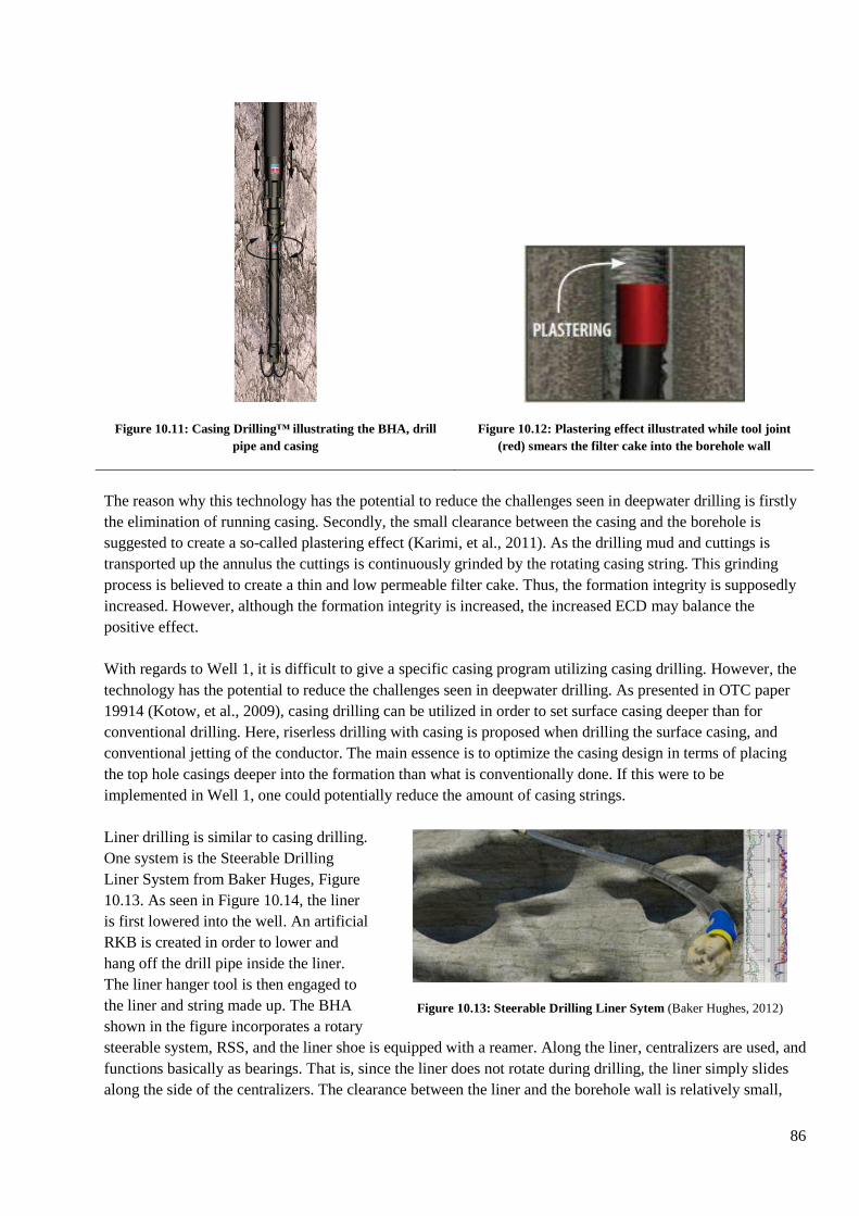
86

Figure 10.11: Casing Drilling™ illustrating the BHA, drill

pipe and casing

Figure 10.12: Plastering effect illustrated while tool joint

(red) smears the filter cake into the borehole wall

The reason why this technology has the potential to reduce the challenges seen in deepwater drilling is firstly

the elimination of running casing. Secondly, the small clearance between the casing and the borehole is

suggested to create a so-called plastering effect (Karimi, et al., 2011). As the drilling mud and cuttings is

transported up the annulus the cuttings is continuously grinded by the rotating casing string. This grinding

process is believed to create a thin and low permeable filter cake. Thus, the formation integrity is supposedly

increased. However, although the formation integrity is increased, the increased ECD may balance the

positive effect.

With regards to Well 1, it is difficult to give a specific casing program utilizing casing drilling. However, the

technology has the potential to reduce the challenges seen in deepwater drilling. As presented in OTC paper

19914 (Kotow, et al., 2009), casing drilling can be utilized in order to set surface casing deeper than for

conventional drilling. Here, riserless drilling with casing is proposed when drilling the surface casing, and

conventional jetting of the conductor. The main essence is to optimize the casing design in terms of placing

the top hole casings deeper into the formation than what is conventionally done. If this were to be

implemented in Well 1, one could potentially reduce the amount of casing strings.

Liner drilling is similar to casing drilling.

One system is the Steerable Drilling

Liner System from Baker Huges, Figure

10.13. As seen in Figure 10.14, the liner

is first lowered into the well. An artificial

RKB is created in order to lower and

hang off the drill pipe inside the liner.

The liner hanger tool is then engaged to

the liner and string made up. The BHA

shown in the figure incorporates a rotary

steerable system, RSS, and the liner shoe is equipped with a reamer. Along the liner, centralizers are used, and

functions basically as bearings. That is, since the liner does not rotate during drilling, the liner simply slides

along the side of the centralizers. The clearance between the liner and the borehole wall is relatively small,

Figure 10.13: Steerable Drilling Liner Sytem (Baker Hughes, 2012)

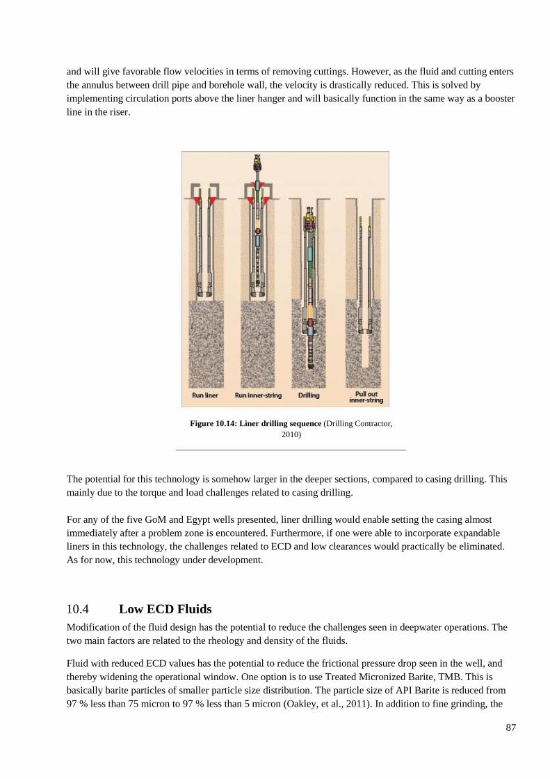
87

and will give favorable flow velocities in terms of removing cuttings. However, as the fluid and cutting enters

the annulus between drill pipe and borehole wall, the velocity is drastically reduced. This is solved by

implementing circulation ports above the liner hanger and will basically function in the same way as a booster

line in the riser.

Figure 10.14: Liner drilling sequence (Drilling Contractor,

2010)

The potential for this technology is somehow larger in the deeper sections, compared to casing drilling. This

mainly due to the torque and load challenges related to casing drilling.

For any of the five GoM and Egypt wells presented, liner drilling would enable setting the casing almost

immediately after a problem zone is encountered. Furthermore, if one were able to incorporate expandable

liners in this technology, the challenges related to ECD and low clearances would practically be eliminated.

As for now, this technology under development.

Low ECD Fluids 10.4

Modification of the fluid design has the potential to reduce the challenges seen in deepwater operations. The

two main factors are related to the rheology and density of the fluids.

Fluid with reduced ECD values has the potential to reduce the frictional pressure drop seen in the well, and

thereby widening the operational window. One option is to use Treated Micronized Barite, TMB. This is

basically barite particles of smaller particle size distribution. The particle size of API Barite is reduced from

97 % less than 75 micron to 97 % less than 5 micron (Oakley, et al., 2011). In addition to fine grinding, the

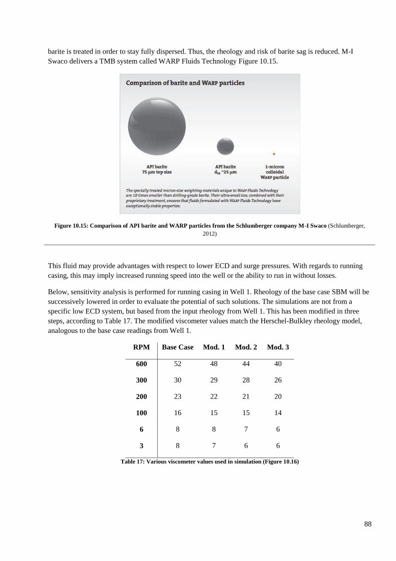
88

barite is treated in order to stay fully dispersed. Thus, the rheology and risk of barite sag is reduced. M-I

Swaco delivers a TMB system called WARP Fluids Technology Figure 10.15.

Figure 10.15: Comparison of API barite and WARP particles from the Schlumberger company M-I Swaco (Schlumberger,

2012)

This fluid may provide advantages with respect to lower ECD and surge pressures. With regards to running

casing, this may imply increased running speed into the well or the ability to run in without losses.

Below, sensitivity analysis is performed for running casing in Well 1. Rheology of the base case SBM will be

successively lowered in order to evaluate the potential of such solutions. The simulations are not from a

specific low ECD system, but based from the input rheology from Well 1. This has been modified in three

steps, according to Table 17. The modified viscometer values match the Herschel-Bulkley rheology model,

analogous to the base case readings from Well 1.

RPM Base Case Mod. 1 Mod. 2 Mod. 3

600 52 48 44 40

300 30 29 28 26

200 23 22 21 20

100 16 15 15 14

6 8 8 7 6

3 8 7 6 6

Table 17: Various viscometer values used in simulation (Figure 10.16)

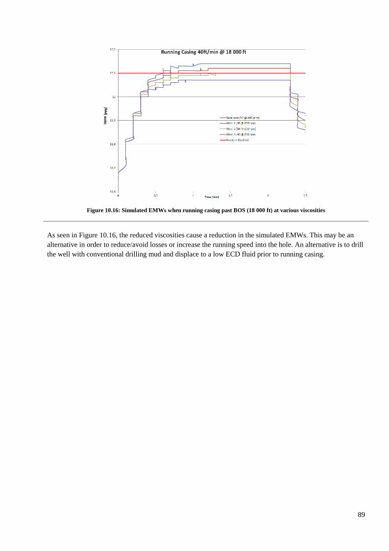
89

Figure 10.16: Simulated EMWs when running casing past BOS (18 000 ft) at various viscosities

As seen in Figure 10.16, the reduced viscosities cause a reduction in the simulated EMWs. This may be an

alternative in order to reduce/avoid losses or increase the running speed into the hole. An alternative is to drill

the well with conventional drilling mud and displace to a low ECD fluid prior to running casing.

90

Conclusions 11

Deepwater drilling is fairly complex and challenging. When combining all effects related to the increasing

water depth it is clear that further development of technology is needed in order to gain access to the

resources in the deepwater frontier. The main conclusions that can be drawn from this thesis are:

There are generally two ways of reducing the problems seen in deepwater drilling and the related low

clearances.

1. Reducing the amount of casing stings and consequently reducing the ECD

2. Reducing the ECD and still maintain a low clearance casing string design

Reducing the amount of casing string can be achieved by:

Dual gradient drilling

Casing drilling (mainly tophole)

Liner drilling (especially deeper sections)

Reducing the ECD can be achieved by:

MPD (reduce fluctuations)

Low ECD fluids (reduce rheology)

Through the study, combined potential solutions were found. These were:

A combined MPD and dual gradient drilling solution

Liner drilling combined with expandable liners

Further conclusions:

Loss of drilling mud is an expensive affair and should be minimized.

Deepwater drilling requirements and practices are also found significant. As seen through the thesis,

these often make the wells un-drillable. Thus, some requirements and practices are not always suited

for deepwater drilling.

91

Abbreviations

BHA Bottom Hole Assembly

BHP Bottom Hole Pressure

BOEMRE Bureau of Ocean Energy Management, Regulation and Enforcement

BOP Blowout Preventer

BOS Base of Salt

CFR Code of Federal Regulations

CCS Continuous Circulation

ECD Equivalent Circulation Density

EMW Equivalent Mud Weight

ESD Equivalent Static Density

FIT Formation Integrity Test

GoM Gulf of Mexico

IADC International Association of Drilling Contractors

LAS Liquid Additive System

LCM Lost Circulation Material

LOT Leak Off Test

MD Measured Depth

MLP Mud Lift Pump

MPD Managed Pressure Drilling

NPT Non-Productive Time

OBM Oil Based Mud

OD Outer Diameter

PDC Polycrystalline Diamond Compact

RCD Rotating Control Device

RKB Rotary Kelly Bushing

RMR™ Riserless Mud Recovery

RPM Revolutions Per Minute

RSS Rotary Steerable System

SBM Synthetic Based Mud

SSC Subsurface Support Center

sg Specific Gravity

SRD Subsea Rotating Device

TD Target Depth

TMB Treated Micronized Barite

TOC Top of Cement

TOS Top of Salt

TVD True Vertical Depth

UiS University of Stavanger

WBS Water Based Mud

WH Wellhead

WOC Waiting on Cement

XLOT Extended Leak Off Test

92

References

Aadnøy B. S [et al.] Advanced Drilling and Well Technology [Book]. - Richardson : Society of Petroleum

Engineers, 2009. - ISBN 978-1-55563-145-1.

Aadnøy B. S Modern Well Design [Book]. - Stavanger : CRC Press, 2010. - Vol. II.

Aadnøy B. S. Geomechanical analysis for deep-water drilling [Conference]. - Dallas : IADC/SPE, 1998. -

IADC/SPE 39339.

Azar J. J and Robello S. G Drilling Engineering [Book]. - Tulsa : Pennwell, 2007. - ISBN-13:978-1-59370.

Baker Hughes Steerable Drilling Liner System [Online] // Baker Hughes. - Baker Hughes, 2012. - May 18,

2012. - http://www.bakerhughes.com/products-and-services/drilling/drilling-services/casing-liner-drilling-

systems/steerable-drilling-liner-system.

BOEMRE Bureau of Ocean Energy Management, Regulation and Enforcement [Online] // History of the

Offshore Oil and Gas Development in Louisiana. - Aeptember 28, 2010. - May 27, 2012. -

http://www.gomr.boemre.gov/homepg/regulate/environ/louisiana_coast.html.

BP BP's oil spill costs grow, Gulf residents react [Online] // Washington Post. - The Associated Press, 11 02,

2010. - 04 05, 2012. - http://www.washingtonpost.com/wp-

dyn/content/article/2010/11/02/AR2010110200474.html.

BP Deepwater Horizon Accident [Online] // BP. - BP, 04 20, 2010. - 10 10, 2011. -

http://www.bp.com/sectiongenericarticle800.do?categoryId=9036575&contentId=7067541.

Breyholtz Ø [et al.] Managed Pressure Drilling: A multi-level control approach [Conference] // SPE

Intelligent Energy Conference and Exhibition. - Utrecht : Paper SPE 128151, 2010. - 978-1-55563-284-7.

Breyholtz Ø [et al.] Managed Pressure Drilling: A multi-level control approach [Conference]. - Utrecht :

SPE, 2010.

CEMEX Cement Manufacturing Process - dry process (process flow) [Online] // Cemexphilippines. -

CEMEX, 2011. - Febuary 20, 2012. - http://www.cemexphilippines.com/ce/ce_cb_cm.html.

Dowell J. David Deploying the World's First Commercial Dual Gradient Drilling System [Conference]. -

Galveston : SPE, 2010. - p. Paper SPE 137319. - 978-1-55563-309-7.

Dowell/Chevron J. David Deploying the World's First Commercial Dual Gradient Drilling System

[Conference]. - Galveston : SPE, 2010. - 978-1-55563-309-7.

Drilling Contractor World’s first steerable drilling liner system successfully field tested offshore Norway

[Online] // Drilling Contractor. - IADC, April 30, 2010. - May 18, 2012. -

http://www.drillingcontractor.org/world%E2%80%99s-first-steerable-drilling-liner-system-successfully-field-

tested-offshore-norway-5375.

Fink J. K Petroleum Engineer's Guide to Oil Filed Chemicals and Fluids [Book]. - London : Gulf

Professional Publishing, 2012. - 1st.

93

Grayson K and DrillingContractor Safe Drilling Operations Come Full Circle [Online]. - 2011. - May 9,

2012. - http://www.drillingcontractor.org/safe-drilling-operations-come-full-circle-10630.

Hannegan Don M SPE DISTINGUISHED LECTURER SERIES [Online]. - 2007. - May 7, 2012. -

http://www.spe.org/dl/docs/2007/HanneganPreso.pdf.

Huatai Foam Concrete [Online] // Made-in-China.com. - 2012. - 03 09, 2012. - http://www.made-in-

china.com/showroom/ht2106/product-detailNbFQHjmwGocC/China-Foam-Concrete.html.

IADC Chevron to Renew Push for Dual-Gradient [Online] // Drilling Contractor. - IADC, September 25,

2009. - April 4th, 2012. - http://www.drillingcontractor.org/chevron_to_renew_push_for_dual_gradient-971.

Janssen E. F. Lecture MOM 450. - Stavanger : UiS, October 19, 2011.

Janssen E. F. Lecture MOM 450 - Flow Assurance. - Stavanger : UiS, October 19, 2011.

Karimi M, Holt C and Moellendick E Trouble Free Drilling with Casing Drilling; a Process Focused on

Preventing the Drilling Problems [Conference] // Paper IPTC 14866. - Thailand : International Petroleum

Technology Conference, 2011.

Karimi M. SPE, Holt C. SPE and Moellendick E. SPE Tesco Trouble Free Drilling with Casing Drilling; a

Process Focused on Preventing the Drilling Problems [Conference] // International Petroleum Technology

Conference. - Thailand : International Petroleum Technology Conference, 2011.

Kotow K. J and Pritchard D. M Riserless Drilling With Casing: A New Paradigm for Deepwater Well

Design [Conference]. - Houston : Paper OTC 19914, 2009.

Kotow K. J and Pritchard D. M Riserless Drilling With Casing: A New Paradigm for Deepwater Well

Design [Journal]. - Houston : OTC, 2009. - Vol. 19914.

Lal M Analysis of Factors Affecting Surge And Swab Pressures [Conference] // Analysis of Factors

Affecting Surge And Swab Pressures. - Houston : Paper SPE/IADC , 1984.

Lal M Analysis of Factors Affecting Surge And Swab Pressures [Conference] // Analysis of Factors

Affecting Surge And Swab Pressures. - Houston : SPE/IADC, 1984.

Lal M Surge and Swab Modeling for Dynamic Pressures and Safe Trip Velocities [Conference]. - New

Orleans : Paper SPE/IADC 11412, 1983.

Lal M Surge and Swab Modeling for Dynamic Pressures and Safe Trip Velocities [Conference]. - New

Orleans : SPE/IADC, 1983. - SPE 11412.

Lea S. H Propagation of Coupled Pressure Waves in Borehole with Drillstring [Conference]. - Calgary :

Paper SPE 37156, 1996.

Lea S. H Propagation of Coupled Pressure Waves in Borehole with Drillstring [Conference]. - Calgary : SPE,

1996. - SPE 37156.

Lubinski A, Hsu F. H and Nolte K.G. Transient Pressure Surges Due to Pipe Movement in an Oil Well

[Book]. - [s.l.] : Revue de I'lst. Fran. du Pet., 1977.

Malloy K. P [et al.] Managed Pressure Drilling: What It Is and What It Is Not [Conference]. - texas : Paper

SPE 122281, 2009.

94

Malloy K. P [et al.] Managed Pressure Drilling: What It Is and What It Is Not [Conference]. - texas : SPE,

2009.

Mitchell R.F Dynamic Surge/Swab Pressure Predictions [Conference]. - [s.l.] : Paper SPE 16156, 1988.

Mitchell R.F Dynamic Surge/Swab Pressure Predictions [Conference]. - [s.l.] : SPE, 1988.

Nelson E. B and Guillot D Well Cementing [Book]. - Houston : Schlumberger, 2006. - 2nd.

Newswise IODP Introduces Technology to Support Deepwater Crustal Drilling [Online] // Newswise. -

Newswide Inc, 04 08, 2009. - 04 08, 2012. - http://www.newswise.com/articles/iodp-introduces-technology-

to-support-deepwater-crustal-drilling.

Oakley D and Conn L Drilling Fluid Design Enlarges the Hydraulic Operating Windows of Managed

Pressure Drilling Operations [Conference]. - Amsterdam : Paper SPE 139623, 2011.

Oakley D and Conn L Drilling Fluid Design Enlarges the Hydraulic Operating Windows of Managed

Pressure Drilling Operations [Conference]. - Amsterdam : Society of Petroleum Engineers, 2011.

Office of the Federal Register Code of Federal Regulations [Book]. - Washington, DC : U.S. Government

Printing Office, 2011. - 978-0-16-088877-9.

Offshore Technology Jack/St Malo Deepwater Project, Gulf of Mexico, United States of America [Online] //

Offshore Technology. - Net Resources International. - 04 07, 2012. - http://www.offshore-

technology.com/projects/jackstmalodeepwaterp/.

Orszulik S. T Environmental Technology in the Oil Industry [Book]. - Hampshire : Oxoid Ltd, 2008. - ISBN

978-1-4020-5471-6.

R.R Israel P. D'Ambrosio, A.D. Leavitt, Schlumberhger, J.M. Shaughnessey BP America and adn J.

Sanclemente Chevron North America E&P Challenges evolve for directional drilling through salt in

deepwater Gulf of Mexico [Online] // Drilling Contractor. - IADC, May 2008. - April 5, 2012. -

http://www.drillingcontractor.org/challenges-evolve-for-directional-drilling-through-salt-in-deepwater-gulf-

of-mexico-1622.

Romanian Society of Rheology Romanian Society of Rheology [Online] // Romanian Society of Rheology. -

2011. - March 15, 2012. - http://www.reologie.ro/an-introduction-to-rheology-and-viscosity/.

Santos H [et al.] Deepwater Drilling Made More Efficient and Cost-Effective: Using the Microflux Control

Method and an Ultralow-Invasion Fluid To Open the Mud-Weight Window [Conference]. - Texas : Paper

OTC 111634, 2006.

Santos H [et al.] Deepwater Drilling Made More Efficient and Cost-Effective: Using the Microflux Control

Method and an Ultralow-Invasion Fluid To Open the Mud-Weight Window [Conference]. - Texas : Offshore

Technology Conference, 2006.

Schlumberger DeepCEM Low-Temperature Cement Slurries [Online] // Schlumberger. - 2012. - March 23,

2012. -

http://www.slb.com/services/drilling/cementing/deepwater_cementing/deepwater_slurries/deepcem.aspx.

Schlumberger DeepCEM Low-Temperature Cement Slurries [Online]. - 2012. - March 23, 2012. -

http://www.slb.com/services/drilling/cementing/deepwater_cementing/deepwater_slurries/deepcem.aspx.

95

Schlumberger Rhino AB At-Bit Reamer [Online]. - 2012. - February 14, 2006. -

http://www.slb.com/services/drilling/tools_services/rhino_reamers/rhino_ab.aspx.

Schlumberger The Oilfield Glossary [Online] // Schlumbeger Glossary Website. - Schlumberger, 2012. - 1

30, 2012. - http://www.glossary.oilfield.slb.com/default.cfm.

Schlumberger WARP Fluids Technology [Online]. - 2012. - May 5, 2012. -

http://www.slb.com/services/miswaco/services/drilling_fluid/df_systems/oil_base/warp.aspx#.

Slanton M. Foamed Cement - Ultra Light and More [Conference]. - [s.l.] : Drilling, 1981. - No. 8, 51-52,15.

SSC Statoil Subsurface Support Centre Drilling Operations [Interview]. - May 20, 2012.

Standards Norway Well Integrity in Drilling and Well Operations [Book]. - Lysaker : Standard Norge,

2004. - 3th.

Statoil ARIS ARIS Management System (Statoil Internal). - May 20, 2012.

Statoil ARIS Management System (Statoil Internal). - May 20, 2012.

Statoil Daily Drilling Report (Statoil Internal). - 2012.

Statoil DBR Daily Drilling Report (Statoil Internal). - 2012.

Statoil Teamsite (Statoil Internal) [Online]. - 2012.

Tesco Casing Drilling [Online]. - 2012. - February 9, 2012. -

http://www.tescocorp.com/bins/casing_drilling_page.asp?cid=2-32.

Transocean Deepwater [Online] // Transocean. - 2012. - 03 17, 2012. -

http://deepwater.com/_filelib/FileCabinet/pdfs/02_TRANSOCEAN_Ch_1-0.pdf.

Transocean Discoverer Americas [Online] // Deepwater. - Transocean Ltd., 2012. - February 2, 2012. -

http://www.deepwater.com/fw/main/Discoverer-Americas-423C16.html?LayoutID=17.

Weatherford Managed Pressure Drilling Promotes Wellbore Stability and Improves Drilling Performance in

HPHT Exploratory Well in Saudi Arabia [Online]. - 2012. - May 5, 2012. -

http://www.weatherford.com/weatherford/groups/web/documents/weatherfordcorp/WFT098423.pdf.

Weatherford Plug Locator System [Online] // Weatherford. - Weatherford, 2012. - May 5, 2012. -

http://www.weatherford.com/dn/WFT078419.

Wikipedia Compressibility [Online]. - April 24, 2012. - May 5, 2012. -

http://en.wikipedia.org/wiki/Compressibility.

Wikipedia Drillship [Online] // Wikipedia. - Wikipedia, May 23, 2012. - May 26, 2012. -

http://en.wikipedia.org/wiki/Drillship.

Wikipedia Hot Clinker [Online] // Wikipedia. - Mars 22, 2008. - Febuary 20, 2012. -

http://nl.wikipedia.org/wiki/Bestand:Hot_Clinker.jpg.

Wikipedia Mass Balance [Online] // Wikipedia. - 2012. - April 27, 2012. -

http://en.wikipedia.org/wiki/Mass_balance.

96

Wikipedia Momentum [Online]. - 2012. - April 27, 2012. -

http://en.wikipedia.org/wiki/Momentum#Conservation_of_linear_momentum.

Wikipedia Wikipedia [Online]. - 2012. - March 15, 2012. - http://en.wikipedia.org/wiki/Emulsion.

WorldOil Exploration Report [Online] // World Oil. - 05 2007. - 04 07, 2012. -

http://www.worldoil.com/May-2007-Regional-geology-of-deepwater-salt-architecture-New-plays-in-the-

GOM.html.

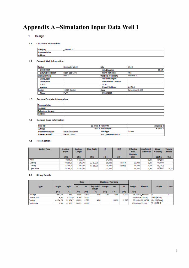
I

Appendix A –Simulation Input Data Well 1

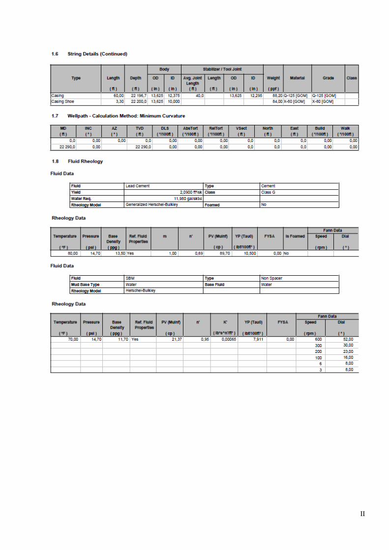
II

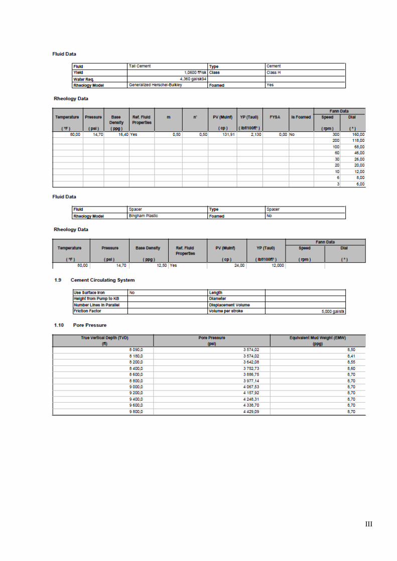
III

IV

V

VI

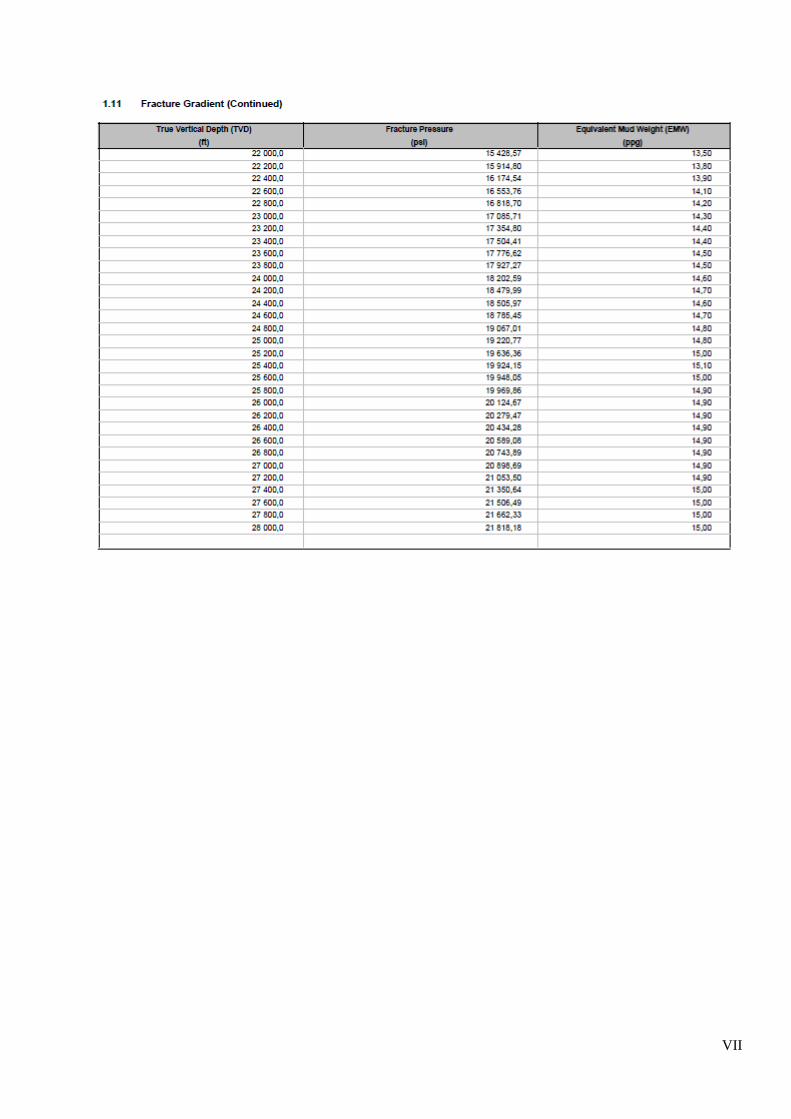
VII

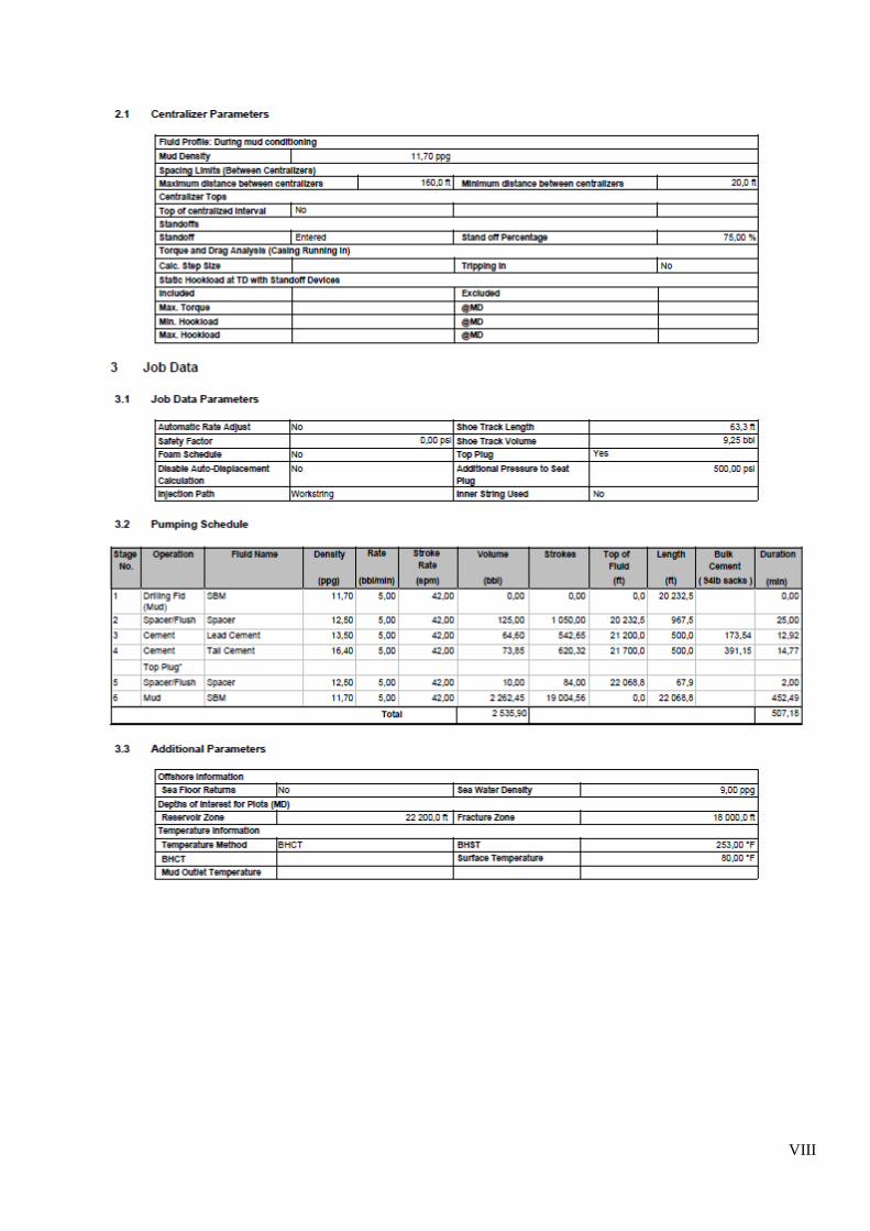
VIII