MASTER’S THESIS - Bibsys · MASTER’S THESIS Study program ... information for the overall heavy light setup design and the development of the operation ... What is the extent

Faculty of Science and Technology

MASTER’S THESIS

Study program/ Specialization:

Master Petroleum Engineering

Specialization Drilling

Spring semester, 2014

Open

Writer:

Eirik Aasberg Vandvik

………………………………………… (Writer’s signature)

Faculty supervisor: Mesfin Belayneh

External supervisor: Harald Syse, Reelwell

Thesis title:

Experimental investigation at heavy light interface mixture of Reelwell ERD

Credits (ECTS): 30

Key words:

ERD, Heavy over light fluid, Reelwell

Pages: 110

+ enclosure: 47 pages

+ Attachment 1 Experimental CD

Stavanger, 13.06.2014

Page : 2

Date : 11.02.14

2

Acknowledgement

I will thank every one of these persons for their immense help, and for taking time in their

busy schedule to help me. Without them this thesis would not have become a reality.

Mesfin Belayneh, Professor of petroleum engineering [UIS].

Harald Syse, Engineering Manager [Reelwell].

Ola M. Vestavik, Chief Technology Officer [Reelwell].

Tom Unsgaard

Vibjørn Dagestad,Senior technical advisor [Wild Well Control].

Laura Belbin Vokey

Sindre Veen Larsen

Page : 3

Date : 11.02.14

3

Abstract

Due to longer offset and large surface area exposure in a reservoir, extended reach drilling

(ERD) is a method which is both cost effective and a well potential during the production

phase. However, the present ERD method envelope is limited to about 12.3km. In order cross

this envelope, the Stavanger based drilling company Reelwell has developed a ultra-long

(>20km) ERD method solution. The method is under development and is in field scale testing

phase. The results show that the technology is feasible and has several advantages over the

conventional methods.

Reelwell uses a range of different features to succeed with increasing the ERD envelope. The

heavy over light concept is one of these.

The concept is comprised of utilizing two different drilling fluids at the same time. Because of

difference in density between the fluids and an inclined wellbore, an interface is created.

This master thesis deals with an experimental study of this heavy light interface and its

behavior when exposed to rotation from the drill string.

In this thesis three test rigs were designed and constructed. Based on the Reelwell operational

and fluid properties, a total of 31 experimental studies were carried out.

The studies investigated several parameters that influenced the dynamics of the heavy light

interface and the resulting mixing zone.

Page : 4

Date : 11.02.14

4

Table of contents

ACKNOWLEDGEMENT .................................................................................................................................... 2

ABSTRACT ........................................................................................................................................................... 3

TABLE OF CONTENTS ...................................................................................................................................... 4

1 INTRODUCTION ....................................................................................................................................... 6

1.1 BACKGROUND ........................................................................................................................................... 6 1.2 PROBLEM FORMULATION ........................................................................................................................... 8 1.3 ASSUMPTIONS ........................................................................................................................................... 9 1.4 OBJECTIVES ............................................................................................................................................... 9

2 REELWELL TECHNOLOGY ................................................................................................................ 10

3 THEORY .................................................................................................................................................... 14

3.1 FORCE OF GRAVITY ................................................................................................................................. 14 3.2 THEORY OF ROTATIONAL FORCE .............................................................................................................. 15 3.3 INTERFACIAL TENSION ............................................................................................................................. 15 3.4 RHEOLOGY MODELS ................................................................................................................................ 16 3.5 FLOW IN ANNULUS WITH PIPE ROTATION ................................................................................................. 20 3.6 THEORY OF FLUID MIXTURE .................................................................................................................... 24

4 EXPERIMENTS ........................................................................................................................................ 28

4.1 DRILLING FLUID PREPARATION AND DESCRIPTION ................................................................................... 29 4.2 EXPERIMENT EQUIPMENT LAYOUT........................................................................................................... 31 4.3 TEST RIG 1# ............................................................................................................................................. 32

4.3.1 Purpose ......................................................................................................................................... 32 4.3.2 Experimental setup ........................................................................................................................ 33 4.3.3 Experiments test rig 1 .................................................................................................................... 34

4.3.3.1 Experiments 1, 2 & 3, effect of inclination ............................................................................................... 34 4.3.3.2 Experiment 4 & 6, Effect of high Yield point ........................................................................................... 36 4.3.3.3 Experiment 5 & 7, Effect of heavy WBM ................................................................................................ 38

4.3.4 Fluid system description ................................................................................................................ 40 4.3.5 Results and analysis ...................................................................................................................... 41

4.4 TEST RIG 2# ............................................................................................................................................. 47 4.4.1 Purpose ......................................................................................................................................... 47 4.4.2 Experimental setup ........................................................................................................................ 48 4.4.3 Experiments test rig 2 .................................................................................................................... 49

4.4.3.1 Experiment 8 & 9, Effect of reduced RPM ............................................................................................... 49 4.4.3.2 Experiment 10, 11, 12 & 13, Effect of heavy light ratio ........................................................................... 51 4.4.3.3 Experiment 14 & 15, Effect of Clockwise (CW) and Anticlockwise (ACW) rotation ............................. 53 4.4.3.4 Experiment 16 & 18, Effect of low RPM ................................................................................................. 54 4.4.3.5 Experiment 17, 19 & 20, Effect of heavy OBM and negative inclination ................................................ 56


4.5 TEST RIG 3 # ............................................................................................................................................ 68 4.5.1 Purpose ......................................................................................................................................... 68 4.5.2 Experimental setup ........................................................................................................................ 69 4.5.3 Experiments test rig 3 .................................................................................................................... 71

4.5.3.1 Experiment 21, 22, 23 and 24, Effect of RPM and pipe size, Matrix 1 .................................................... 71 4.5.3.2 Experiment 25, Effect of low viscous light fluid ...................................................................................... 73 4.5.3.3 Experiment 26, 27, 28 and 29, Effect of RPM and pipe size, Matrix 2 .................................................... 74 4.5.3.4 Experiment 30 and 31, Effect of negative inclination ............................................................................... 75


Page : 5

Date : 11.02.14

5

4.6 VISCOMETER TEST RIG ............................................................................................................................. 92 4.6.1 Purpose ......................................................................................................................................... 92 4.6.2 Experimental setup ........................................................................................................................ 92 4.6.1 Viscometer experiment 1 and 2 ..................................................................................................... 93 4.6.2 Fluid system description ................................................................................................................ 94 4.6.3 Results and analysis ...................................................................................................................... 95

5 DISCUSSION ............................................................................................................................................. 97

6 CONCLUSION ........................................................................................................................................ 110

ABBREVIATIONS ........................................................................................................................................... 111

REFERENCES .................................................................................................................................................. 112

APPENDIX A – EQUATIONS ........................................................................................................................ 114

APPENDIX B – REELWELL TECHNOLOGY ............................................................................................ 115

APPENDIX C – TEST RIG CONSTRUCTION AND GENERAL SPECIFICATIONS ........................... 120

APPENDIX D – EQUIPMENT/TOOLS ......................................................................................................... 138

APPENDIX E – LIST OF CHARTS ............................................................................................................... 149

APPENDIX F – LIST OF FIGURES .............................................................................................................. 150

APPENDIX G – LIST OF GRAPHS ............................................................................................................... 152

APPENDIX H – LIST OF TABLES ................................................................................................................ 154

ATTACHMENT – EXPERIMENTAL CD .................................................................................................... 157

Page : 6

Date : 11.02.14

6

1 Introduction

This thesis discusses the study of heavy light interface mixture phenomenon. The author

designed and constructed experimental rigs at smaller and larger scales. The study is new by

its very nature. Various fluids to be used for Reelwell methods were considered for the

analysis. In order to describe the mixture phenomenon, theories were reviewed to calculate

the fluid properties. The study was part of Reelwell technology, which the thesis result gives

information for the overall heavy light setup design and the development of the operation

procedure.

1.1 Background

The oil industry has always looked for cheaper and more efficient ways of drilling oil wells.

One solution has been to drill longer and more complex wells that cover a larger drainage

area. This technique is generally called Extended Reach Drilling (ERD) and involves drilling

long horizontal directional wells. The main purpose of ERD is to reduce the number of

installations needed to reach oil and gas reserves (see figure 2).

Figure 1 is the ERD drilling envelope. The current maximum record is the well drilled in

2011 in Russian. The well is located in Sakhalin-1 - TMD 12345 m & 11475 m horizontal

offset [06]. The main challenging with the conventional drilling is torque and drag that limits

drilling from reaching to a longer offset.

Throughout the years drilling technology has evolved and allowed ERD wells to grow longer.

The main challenges for ERD wells are the mechanical loads on the drill string (especially

friction induced torque and drag), hole cleaning and managing downhole pressure. Ever since

the invention of steerable mud motors, directional drilling has been pushing its boundaries.

Figure 1: Extended reach drilling envelope. [07]

Page : 7

Date : 11.02.14

7

These challenges limit the range of conventional drilling. To solve them different companies

have presented unique solutions. Reelwell is one of these companies.

Reelwell TM

is a company established with the main goal of drilling and competing over 20

km MD ERD well. To reach this goal they have invented the Reelwell Drilling Method

(RDM), which uses a dual conduit drill string. The drill string pumps drilling fluid through

outer inner pipe and sucks it in through the inner drill pipe together with cuttings. According

to Reelwell, RDM drastically decreases torque and drag, which again allows for longer ERD

wells.

The extended reach provided by the RDM decreases the amount of equipment needed to

recover hydrocarbon resources from a field. Figure 2 shows a comparison between

conventional and Reelwell drainage area [R02]. As shown, the Reelwell technology can

replace several platforms and thereby reduce overall cost.

Figure 2: Comparison of Conventional drainage area vs. Reelwell drainage area. [R02]

A main feature of their method is called the “heavy over light” concept (see figure 3) which

involves using two separate drilling fluids, one heavy and one light. The heavy fluid is

positioned in the annulus and lies stagnant, while the light fluid is circulated in and out of the

dual conduit string and provides hole cleaning. Gravity ensures the position of the two liquids.

Heavy light technology will be explained in more detail later in the thesis.

Figure 3: Displays Reelwells heavy over light concept. [R02]

Page : 8

Date : 11.02.14

8

1.2 Problem formulation

The Reelwell heavy light method drills the well with two different density mud systems, a

heavy and a light, which forms an interface as shown in the figure 4. These two systems have

different properties and purposes, and should remain separate to secure wellbore integrity,

hole cleaning and other drilling related purposes. Because of the low inclination the heavy

light interface will expose a significant area of the wellbore. This leads to mixing between the

two fluids when drilling is engaged

The main question of this thesis is formulated:

What parameters affect the mixing rate and to what degree?

This problem will be dealt with in this thesis.

Other questions to be addressed in this thesis are:

What forces keeps the liquids separated or engages mixing?

What are the dynamics of the mixing of the mud system?

What is the extent of the mix zone?

What mixing rate will the interface travel with?

Will the current Reelwell fluid properties have a positive or negative effect for the

interface movement?

Figure 4: Illustrates Reelwells heavy over light method. [R02]

Page : 9

Date : 11.02.14

9

1.3 Assumptions

Under laboratory scale it is difficult to simulate the field conditions. However, the laboratory

scale test attempt to investigate the heavy/light interface phenomenon under simplified

experimental conditions. Therefore, the following assumptions and conditions are considered:

Experiments performed at room temperature and pressure

Figure 5, inclination readings are relative to the horizontal plane.*

Cutting effects are not considered in the experimental setup

The effect of pressure at the drilling bit and the pressure delivered by the heavy

fluid assumed to cause the interface at static condition. This means that the

interface is not moving due to the change in pressure. Therefore, this assumption

describes the experimental setup.

Flow of the light fluid is not taken into account. The fluid is assumed to be

stagnant.

The experimental wellbore is smooth and without cavities or gaps.

Wellbore instability problems such as, but not limited to unconsolidated

formations and shale collapse, are not taken into account, and will not be a part of

the experimental systems.

Pipe eccentricity, buckling and other mechanical malfunctions will not be

simulated.

* = Inclination angle is normally relative to the vertical axis in conventional drilling. For

convenience inclination is in this thesis relative to the horizontal plane.

1.4 Objectives

The objective of this thesis is to study/analyze

the effect of different rheology properties at the interface

the effect of change in density between the light and the heavy

the effect of OMB's and WBM's at the interface

the effect of the change two OBM’s of various density and rheology

the effect of well inclination

the effect of RPM on mixing interface

the effect of varying distance between wellbore and pipe

the effect of different pipe sizes

Figure 5: Figures illustrating how inclination is perceived in the thesis. [04]

Page : 10

Date : 11.02.14

10

2 Reelwell technology [Information about Reelwell and its technology are taken from references [R01, R02, R03]. For more detailed

information about Reelwell technology, see Appendix B]

The drilling technology company Reelwell was founded in 2004 by Dr. Ing. Ola M. Vestavik.

They specialize in groundbreaking and innovative drilling solutions for the oil and gas

industry. The award winning company’s main office is located in Stavanger and is currently

employing 17 persons. Reelwell is considered a cutting edge company within ERD and with

their Reelwell Drilling Method (RDM) a future force to be reckoned with in development of

new ERD procedures.

Reelwells RDM is a new drilling method, developed and refined for use in the oil and gas

industry in recent years. It is a multi-purpose drilling method equipped with a unique flow

arrangement. RDM is based on using a conventional drill string combined with an inner string

to form a dual conduit drill string (see figure 6 on next page). This configuration allows the

return fluid, saturated with drill cuttings from the bottom of the well, to be transported back

through the inside of the drill string.

Potentially RDM will increase the envelope for EDR, due to several reasons:

Elimination of the dynamic Equivalent Circulating Density (ECD) gradient, since the

ECD is screened from the formation.

The use of a flotation technique (see Heavy over light) of the drill string will reduce

Torque and Drag.

Optional Hydraulic Weight on Bit (WOB), due to a piston encapsulated drill string.

With these features, RDM can be a dominating factor in ERD in the future.

Page : 11

Date : 11.02.14

11

Heavy over light

The heavy over light concept is one of the main features of Reelwells RDM. A “hook” shaped

bore is drilled (see figure 6) to allow the usage of two fluids with different densities in one

wellbore. The “hook” shaped well path is made to create a 1 degree inclination in the

horizontal section. This is done to maintain the position of the fluids and to prevent u-tubing.

In the heavy light scenario, a heavy fluid lies stagnant in the annulus, while a light fluid is

pumped through the outer drill pipe and out through the drill bits nozzles. The light drilling

fluid and the cuttings are sucked into the drill string again through holes approximately 100

meters from the drill bit, and transported to the surface in the inner drill string. When drilling

advances, more heavy fluid is pumped into the annulus to secure the correct heavy light

interface position and wellbore stability.

The main purpose of the heavy light concept is to try to keep the drill string buoyant. This

will drastically reduce the friction between the wellbore and the drill string, which again will

reduce the torque and drag.

The heavy light setup accomplishes buoyancy by utilizing two methods:

i. Using the density difference between the two liquids to create buoyancy. The higher

the difference, the higher the buoyancy.

ii. Using aluminum as drill pipe material instead of steel (optional). Aluminum has 1/3

of the density of steel, which makes aluminum drill pipes more buoyant than their

steel opposites.

Figure 6: Displays the heavy light setup with all RDM components. [R03]

Page : 12

Date : 11.02.14

12

The effect of the density difference is displayed in the graphs and tables below. Higher

density difference leads to a fully buoyant string that drastically reduces drag.

Well annulus (heavy) fluid density [sg]

Active (light)fluid density [sg]

Density difference Heavy – light [sg]

No buoyancy 1.20 1.20 0

Partly Buoyancy 1.56 1.20 0.36

Full Buoyancy 1.75 1.15 0.50

Table 1: Effect of density difference on drill pipe buoyancy. [R03, 02]

Graph 1: Displays buoyancy effects on drag in a RDM drilling scenario. [R03]

Page : 13

Date : 11.02.14

13

Graph 2 shows a combination of having a difference in density and the usage of aluminum

pipe. As seen, the combination results in very low torque numbers. This again allows for an

extended horizontal reach, as illustrated in the graph.

With a fully buoyant drill string, the heavy over light concept may help Reelwell to

accomplish their 20 km goal.

Graph 2: Shows the effect of buoyancy and drill pipe material has on torque. [R03]

Page : 14

Date : 11.02.14

14

3 Theory [Information about the theory is obtained from references listed under Theory in the reference list. All equations

used in the theory is displayed in Appendix A]

The fluids in Reelwells heavy over light principle is subjected to external forces when

undergoing a drilling procedure. Together with the fluid rheology, they govern the behavior

pattern of the interface. The two major forces are the force of gravity and the force of rotation,

while dominating factors of the fluid rheology are assumed to be viscosity and density.

In this subsection, these forces and fluid properties will be clarified and explained so that

experiment outcome can be predicted.

3.1 Force of gravity

The Reelwell Drilling Method heavy over light is based on Newton's theory of gravity. The

theory states that:

“Every point mass attracts every single other point mass by a force pointing along

the line intersecting both points. The force is proportional to the product of the two

masses and inversely proportional to the square of the distance between them".

Using the theory of gravity, the gravitational pull on Reelwells heavy over light system can be

expressed by this equation:

(1)

The equation shows that the gravitational force between the earth and the heavy liquid is

higher than for the light liquid. The heavier fluid will therefore try to position itself beneath

the light fluid as fast as possible (depending on the difference in density).

Reelwells heavy over light method depends on these gravitational forces to be sufficient

enough to keep the two fluids separated.

Page : 15

Date : 11.02.14

15

3.2 Theory of rotational force

As a drill string rotates with angular velocity , the larger deformation is obtained at wall of

the drill string and reduces as we go to the outer cylinder as shown in figure 7. The

configuration describes the experimental rig presented in chapter 4. Therefore, one can

assume that fluid deformation the experimental rigs can be such as this.

The shear rate and the angular velocity for this configuration are given as [T01]:

(2)

3.3 Interfacial tension

Surface tension is a property caused by the different intermolecular forces exerted at the fluid

interface. The main forces involved in interfacial tension are adhesive forces (tension)

between the liquid phases or liquid phase with either a solid or gas phase. The interaction

occurs at the surfaces of the substances involved, i.e. the corresponding interfaces.

Cohesive forces are the intermolecular which cause a tendency in liquids to resist separation.

The intermolecular forces include those from hydrogen bonding and Van der Waals forces.

During emulsification process, interfacial tension also plays an important role. Emulsification

is a heterogeneous system, consisting of at least one miscible liquid dispersed in another in

the form of droplets. In our case, the light drilling fluid mixes with the heavy drilling fluid in

the mixture zone. Since two systems are in contact by the action of the rotational force, they

will tend to mix.

Figure 7: Bottom view of a rotation drill pipe in a wellbore. [04]

Page : 16

Date : 11.02.14

16

3.4 Rheology models

[Information about the rheology models is taken from reference [T02].]

The rheology is the study of the deformation and flow of fluids. In the literature there are

several rheology models to describe the behavior of the fluids. The rotational and axial

motions of the drill string have effects on the fluid rheology properties, which are key

parameters for the determination of fluid flow patterns. The rheology models categorizes as

Newtonian and non-Newtonian. The Non-Newtonian models are Bingham plastic, Power law,

API, Herschel-Buckley, Unified, and Robertson-Stiff. These models approximate fluid

behavior. Graph 3 illustrates the shear stress-shear rate behavior of the models.

A Fann viscometer is usually used to measure shear stress and shear rate. The apparatus is

shown in Appendix C.

The viscometer is also used to measure rheology properties as gel strength and viscosity of

various fluids. A range of speed between 300 and 600 rpm is most common but instruments

with RPM ranging from 3, 6, 100, 200, 300, 600 are used. The setup of the viscometer is

made up out of an inner bob and an outer rotating steel cylinder. When the outer cylinder

starts to rotate, the viscous drag of the fluid pulls the bob in the direction of rotation. Torque

is created on the bob, which is measured by a spring and a dial which are connected to the

bob. The torque which is strained on the bob is called shear stress ( ) and the rotational speed

of outer cylinder is called shear rate ( ).

When converting laboratory data units to field engineering units, the measured data should be

multiplied with the conversion factors shown below

Graph 3: Displays the models shear stress-shear rate behavior. [T03]

Page : 17

Date : 11.02.14

17

Rheology properties

The rheological properties of fluid are determined from Fann measurements. The three

parameters are sometimes used to better describe fluid behavior. In this thesis, the Newtonian

and non-Newtonian (Bingham plastic and Power law) models are considered when describing

the rheological properties of fluid systems. From Bingham plastic fluid, PV (plastic viscosity)

and YP (Yield point) parameters are measured from the 600 and 300 RPM viscometer

readings. Similarly from the viscometer reading, for power-law fluid model, exponent (n) and

consistency (k) parameters are also calculated. However, there is also three parameter

rheology models used to describe the behavior of fluid system. These are Herschel-Bulkley

and Robert and Stiff model.

Newtonian fluid

Newtonian fluid is one parameter rheology mode. According to Newtonian model, the shear

stress is directly proportional to shear rate. The model described a fluid system which doesn’t

contain solid particles and at zero shear rate the fluid is able to flow. The Newtonian fluid has

a constant viscosity at any shear rate. Newtonian model describe fluid systems such as water,

glycerin, oil, light hydrocarbon. The fluid system can be described by [T04]:

(3)

Where:

- viscosity

- shear rate

Non-Newtonian fluid

A fluid that can’t be described by the Newtonian fluid model is called a non-Newtonian fluid.

Examples of non-Newtonian fluids include slurries, pastes, gels, polymer solutions etc.

Non-Newtonian fluid can be generally classified as:

Thixotropic: Fluid exhibits decreased viscosity with stress over time

Rheopectic: Fluid exhibits increased viscosity with stress over time

Shear thinning: Fluid exhibits decreased viscosity with increased shear rate

Dilatant or shear thickening: Fluid exhibits viscosity increases with increased shear

rate.

Page : 18

Date : 11.02.14

18

Bingham plastic

The Bingham plastic rheology model is commonly used in the industry to describe flow

behavior of many types of muds. The Bingham plastic model is a two parameter model.

According to the model, the fluid system exhibits constant viscosity at any shear rate. At zero

shear rates, the fluid system requires a certain external pressure in order to be set into flow.

Mathematically the shear stress-shear rate can be described as:

(4)

Where:

- Plastic viscosity:

- shear rate:

- Yield point:

The plastic viscosity part is the measure of fluid-fluid, fluid-particle, or particle-particle

friction. For faster drilling operation, the plastic viscosity (PV) needs to be as low as possible.

The PV can be obtained by minimizing colloidal solids.

The YP part of the friction is due to an electrostatic force of attraction or repulsion between

charges or ions within the drilling fluid system. The drilling fluid needs to have high enough

YP in order to carry cutting out of the hole.

Plastic viscosity (PV) is calculated with the following equation:

(5)

The yield value can be determined with the following equations:

(6)

(7)

Page : 19

Date : 11.02.14

19

Power law

Unlike the Bingham model, the viscosity of fluid decreases as the shear rate increases. This

model describes drilling fluid such as water based polymer fluid.

Mathematically, the Power-law for fluids is described as [T04]:

(8)

k - is the consistency index. It represents the average viscosity of the drilling fluid for

the overall shear rate.

n - is the flow behavior index. It’s a rheological property of matter related to the

cohesion of the individual particles of a given material, its ability to deform and its

resistance to flow.

(9)

(10)

Page : 20

Date : 11.02.14

20

3.5 Flow in annulus with pipe rotation

Ramadan and Miska presented theoretical and experimental work on the RPM effect on the

drilling fluid rheology [T05]. Figure 8 illustrates the flow behavior under axial and rotational

monitions.

Figure 8: Helical flow of YPL fluid in concentric annulus. [T05]

It is reported that for most drilling fluids, the yield power law rheology model describes the

rheology behavior more accurate than the Bingham plastic and power law model. The model

is given as (Unified model):

2,5.8

m

yw k (11)

Where k is consistency index and m is fluid flow index. Assume that the axial flow is in the

presence of the drill string rotation. The shear velocity will be the resultant of the axial and

the rotational speeds, given as (Ramadan and Miska, 2008):

2,5.9

2

rz

2

z (12)

Where,

*

and z

*

are the wall shear rates of axial tangential flows. Applying the narrow slot

approximation, the average axial shear rate at the wall can be estimated as: 2.5.10

io

z

*

DD

U12

N3

N21

(13)

R

Page : 21

Date : 11.02.14

21

The rotational shear rate at the inner pipe wall can be approximated as:

2.5.11

io

i*

DD

D

(14)

The flow behavior index, N is calculated using the following equation:

2.5.12

2x1m

mx

1m

11

1m2

m3

1N2

N3 (15)

Where

wy /x

Angular velocity

Suppose we have a yield power law fluid and it flows with an axial and rotational motion.

Then we can calculate the angular velocity,

RPM60

2 (16)

Calculate the axial velocity:

A

Qv (17)

Calculate mean tangential velocity, Vr:

ir rV . (18)

Page : 22

Date : 11.02.14

22

Reynolds number

When measuring the pressure drop in the string and the annulus, it is crucial to determine

which of the three flow regimes which is present. The Reynolds number can be used to figure

out the flow regime. The Reynolds number “Re” is a dimensionless number. It is a function

of the ratio of inertial forces to viscous forces. The number quantifies the relative significance

these two types of forces for given flow conditions. The Reynolds numbers are used to

categorize if the flow regimes are in laminar, transitional or turbulent flow. The Reynolds

numbers is for this thesis expressed by equation:

reff vDslot

785Re, (19)

Where

pweff DDD (20)

r

pw

pV

DDYP )(5 (21)

And

is the effective diameter (m)

is the density of the fluid (kg/m³)

Vr is the rotational velocity of the drill pipe (SI units: m/s)

Other factors used in the equations are described as:

is the inside diameter of the annulus (m)

is the outside diameter of the drill pipe (m)

is the plastic viscosity of the fluid (Pa·s)

is Yield point (lbf/100sq ft)

Flow patterns corresponded to Reynolds number:

o Laminar flow: Re < 2000

o Transitional flow: 2000 < Re < 4000

o Turbulent flow: Re > 4000

Page : 23

Date : 11.02.14

23

Fluid flow patterns /regimes

Figure 9 illustrates the three flow regimes.

Laminar flow = Characterized by parallel fluid lines that flow relative to each other and

velocity that increases towards the center of the stream. Laminar flow typically occurs when

the fluid is very viscous and the flow velocity is low. In laminar flow the motion of the

particles of fluid is highly organized, with all the particles moving in straight lines parallel to

the pipe walls.

Transitional flow = A mixture of laminar and turbulent flow, with laminar flow near the

edges of the pipe and turbulence in the middle.

Turbulent flow = Characterized with chaotic motion and high velocity. In turbulent flow, the

fluid layers mix together and create a mixture of all liquids in the pipe. Turbulent flow has

advantages in cutting removal (conventional drilling method) because the turbulence helps to

keep the particles in suspension.

Figure 9: Displays the three flow regimes. [T02]

Page : 24

Date : 11.02.14

24

3.6 Theory of fluid mixture

Since there are only two forces (gravity and rotation) working on the heavy and light fluids,

heavy light interface and mixing zone development can be predicted. If we assume that the

two fluids are miscible, have the same properties (except density) and are contained within a

positive inclined system, one may observe the following:

With only the force of gravity affecting the system, the heavy light interface should be

parallel with the horizontal plane (see figure 11 on next page for illustration).

With the force of gravity and rotation affecting the system, the mixing interface would

be normal to the wellbores inclination () (see figure 12 on next page for illustration).

The length of the mixing zone will not be longer than the length of the wellbore that is

exposed to the mixing zone (see equation 24 below).

These assumed observations are quantified and illustrated below.

The length of the mixing zone was calculated using Pythagoras:

(22)

(23)

Insert equation 22 into 23 results in:

(24)*

* = Not applicable for horizontal or

negatively inclined wellbores.

Where

= Length of mixing zone

= Length of heavy light interface

= Diameter of wellbore

= Wellbore inclination

Figure 10: The heavy light fluid scenario displayed with the applicable component names and setup. [04]

Page : 25

Date : 11.02.14

25

Force of gravity

When the only force acting on the liquids is gravity, the two fluids will follow the path of

least resistance and create a horizontal interface as displayed in figure 11.

No mixing will occur in this scenario. The fluids and the interface will remain stagnant until

an additional force is added.

Force of gravity and rotation

When rotational force is added, the heavy light interface moves and forms a vertical

boundary, which is relative to the wellbore wall. Figure 12 illustrates this phenomenon.

Since no axial force is provided by the force of rotation from the drill pipe, we can assume

that no axial movement of the mixing zone will occur.

Figure 11: Showing the assumed heavy light interface when only the force of gravity affects the fluids. The dashed lines

running throughout the figure represent the drill pipe. [04]

Figure 12: Showing the assumed heavy light interface when the forces of gravity and rotation affect the fluids.

The dashed lines running throughout the figure represent the drill pipe. [04]

Page : 26

Date : 11.02.14

26

Density mixture (light + heavy viscosity mixture)

During kick influx (hydrocarbon or formation fluid), the influx will be mixed with drilling

fluid. This modifies the density, the viscosity and the velocity of the fluid. Density is an

important parameter that affects both the friction loss and hydrostatic pressures. Assuming

that a certain concentration of mud mixed with the gas, the mixture density is given as

(Steinar Evje and Kjell Kåre Fjelde, 2002 [T06]

):

(25)

(7)

Phase volume fraction of gas and liquid, g,l is defined as:

(26)

Similarly, the mixture between heavy and light can be determined by equation 25 and the

result is illustrated as in graph 4. Remember that the mud density,m is also a function of

temperature and pressure.

The hydrostatic pressure is determined by the average density of mud and cuttings in the

annulus. The frictional pressure losses depend on the wellbore geometry, the flow regimes,

the pipe rotation and the drill string dynamics.

0

0,1

0,2

0,3

0,4

0,5

0,6

0,7

0,8

0,9

1

0 0,1 0,2 0,3 0,4 0,5 0,6 0,7 0,8 0,9 1

De

nsi

ty f

ract

ion

of

he

avy

flu

id in

mix

ing

zon

e

Volume fraction of light fluid in mixing zone

Density distribution in mixing zone

Only heavy fluid

Only light fluid

Graph 4: Displaying the distribution of density in the mixing zone. [02]

mgggmix )1(

gl 1

Page : 27

Date : 11.02.14

27

Effect of cutting concentration

The effective density of the mud can be determined from the fluid-fluid mix and cutting. This

can be derived based on mass balance and given as:

2.5.14

vcuttingvmixmudeffective CC )1( (27)

Where Cv is cutting concentration in the annulus, mix is the density of drilling fluid, and

cutting is the density of cutting.

Viscosity mixture

Steinar Evje and Kjell Kåre Fjelde, 2002) also defined the mixture viscosity as [T06]:

(28)

is the heavy and light phase viscosities

(29)

Page : 28

Date : 11.02.14

28

4 Experiments [All experiments were conducted following the HSE standards of UIS and the Institute of petroleum]

To learn more about the interface mixture phenomenon, a series of experiments was

conducted to observe the mixing and spread of the mixing zone between the light and heavy

fluids. Every experiment was documented with pictures and videos, which are included in the

thesis or in the attached CD as mp4 files.

To be able to conduct a large number of experiments, differently sized test rigs were made.

Small scaled experiments allowed for more trial and error, and helped to sort out the

importance of the different parameters. The larger scaled experiments would try to simulate

the actual conditions and parameters of the RDM heavy over light.

All experiments used the horizontal plane as reference and as baseline for the measured

inclination (see Assumptions, section § 1.3)

Reelwell heavy light scenario

Reelwell has given a heavy light scenario, which this thesis will address and use as a

benchmark. The following properties are given:

Inclination: 1o

RPM: 20 – 200

ROP: 5 – 10 m/h

Mud type SG [kg/l]

PV [CPS]

YP [lbs/100ft²]

LSR YP [lbs/100ft²]

HTHP Fluid loss [ml/30min]

Drill solids [%]

Activity [ ]

O/W ratio [%]

El. Stability [Volt]

Heavy OBM 1,40 30 20 - - 0 0,6 80/20 1000

Light OBM 1,10 20 20 - - 0 0,6 80/20 1000

Table 2: Reelwell heavy light fluid properties. [R05]

Page : 29

Date : 11.02.14

29

4.1 Drilling fluid preparation and description

For the heavy part of the system, an 80/20 oil water ratio (OWR) drilling fluid was prepared

in order to meet the desired Reelwell requirements. The drilling fluid was prepared according

to MI-SWACO fluid formation procedure and the ingredients are products of MI-SWACO.

The rheology and the physical properties of the fluid are measured.

The measurements were carried out at room temperature and pressure. However the properties

are depending on the thermodynamics states.

For the light part of the system, food oil was used, having a density of 0.9sg. The density

difference at the interface was designed to be 0.3sg. The main reason we didn’t prepare a light

mud, is because of barite discoloration. The discoloration made it impossible to obtain a

contrast between the heavy and light fluid. It made it difficult to monitor the dynamics of the

mixing zone.

To investigate the effect of density contrast, we vary the density of the heavy mud by adding

an appropriate Baryte in order to obtain the desired density.

The drilling fluid consists of primarily three phases (oil, water, particles). The additives are

Emulsifiers, Viscosifiers and Filter control substances.

The preparation procedure is displayed in Experimental fluids recipe and the viscosity

information are shown in the individual test rigs Fluid system description (subsections § 5.3.4,

5.4.4, 5.5.4 and 5.6.4).

Page : 30

Date : 11.02.14

30

Experimental fluids recipe

When conducting experiments with the four test rigs, certain customized liquids were made to

fit these experiments purposes. The recipes and preparation procedures of these liquids are

displayed below.

Syrup 1 and 2

The two Syrup fluids were mixed with the trial and error method. Commercial syrup was

added to water until desired density was reached.

Bentonite 1

Bentonite 1 was made by adding 50 g of bentonite to every 1000 g of water.

Baryte 1

The heavy WBM was made by adding a pre calculated amount of barite (see equation 30) to

the Bentonite 1.

OBM 1, 2 and 3

Product name Use 80/20 OBM Mixing time

EDC 95/11 Base Fluid 440

Paramul Emulsifier 20

Parawet Wetting agent 8 5 min

Lime(Hydratkalk) pH modifier 20 5 min

Water (mix water + salt separately and

add the brine mixture) 137

CaCl2 (mix water + salt separately and

add the brine mixture) Osmotic control 37

10 min

Versatrol M Fluid loss control 10 5 min

Benton 128 Viscosifier 9 5min

Barite (All Grades) Weighting agent 341 25 min

Table 3: Mud formulation and ingredients. [05]

Amount of needed Barite was calculated using equation

30)

Where

mp: Mass of particles (barite)

mp: Mass of fluid

p: Density of particles (4.2sg)

f: Density of fluid

ff: Density of finished fluid

Page : 31

Date : 11.02.14

31

Diesel and Rapeseed oil mixture

The light fluid was made using the trial and error method. The goal was to make a light liquid

with the same properties as used in Reelwells proposed fluid scenario. A diesel rapeseed oil

ratio was first mixed and then tested with a Viscometer to see if the rheology matched.

Results of the trial and error are shown in the table below:

Nr. Diesel Rapeseed ratio PV (cP)

1 4:1 6

2 2:1 8,5

3 1:1 14,5

4 4:5 17

5 2:3 20

Table 4: Trial and error diesel rapeseed ratio.

A diesel rapeseed ratio of 2:3 gave the correct plastic viscosity (PV) according to Reelwells

fluid scenario.

4.2 Experiment equipment layout

Several different equipment, ingredients and tools were used prior, during and after the

experiments. They can be divided into four main groups:

Experiment tools: Equipment/tools used to conduct the experiments.

Fabrication equipment: Tools and equipment used under the fabrication process of

the various test rigs and their components.

Measuring equipment: Devices used to measure, test, inspect or examine parts or

components in order to determine compliance with required

specifications and/or tolerances.

Safety equipment: Equipment used to protect individuals and personnel from

hazardous conditions faced under experiments.

For more info the four groups is displayed in Appendix D, containing descriptions and

pictures of used equipment and tools.

Page : 32

Date : 11.02.14

32

4.3 Test rig 1#

4.3.1 Purpose

The first test rigs purpose was to determine how different fluid parameters would affect the

mixing of the heavy and light fluid. A small scale test rig was built with the intention of easily

being able to execute a high number of experiments. The rig allowed for easy and

uncomplicated testing of parameters such as:

Inclination

Viscosity

Yield point

Heavy light density differences

More realistic environments would be tested in a later part of the experimental phase.

Page : 33

Date : 11.02.14

33

4.3.2 Experimental setup

[See Appendix C – Test rig construction and experiment execution, test rig 1 for detailed information about

construction and fabrication of test rig 1]

Rig # 1 is a 0,515 m length by 29,5 mm diameter well. In this rig a wood bit/blade, 14 mm

width and 153 mm length, was rotated in the light fluid. It would represent a very simplified

drill pipe. The tip of the blade was 28 mm away from the heavy/light interface (in vertical

position) before the execution of the experiments. The test rig is shown in picture 1 below.

Wellbore

Acrylic pipe Length (mm) 515

ID (mm) 29,5

OD (mm) 39,7

Drill pipe

Wood

bit/blade

Length (mm) 153

Size (mm) 14

Table 5: Test rig 1# setup specifics.

Picture 1: Test rig 1 # layout with used equipment positioned for a test of feasibility of future

experiments. The acrylic pipe displayed has an inclination of 3,3o relative to the horizontal plane. The

wood bit is as showed mounded trough the sponge plug into the drill. Weights are placed on both

stands to ensure stability. [01]

Page : 34

Date : 11.02.14

34

4.3.3 Experiments test rig 1

4.3.3.1 Experiments 1, 2 & 3, effect of inclination

The main purpose of the first experiments was to see how the inclination of the test rig would

affect the propagation of the mixing zone. The experiments objective was also to test the

durability and rigidness of the rig. Stability and minimization of vibrations were also

important factors during the execution of experiments 1, 2 and 3.

Used equipment

[See Appendix D for detailed information about used equipment and tools]

The equipment/tools used in experiment 1, 2 and 3 are listed in Used equipment test rig 1,

Appendix C, except for these modifications:

Food dye (green)

iPhone 4 (Ex. 1 & 2)

GoPro Hero 2

Experiment specifications

All three experiments were conducted using water mixed with green food dye as the light

fluid, and syrup 1 as the heavy fluid. Because both liquids are water based, they are miscible

and can be mixed. The added food dye helped distinguish the heavy and light liquid, as well

as illustrate the distribution of the mixing zone. As shown in the experimental setup, the

mixing for test rig 1# was done by using a wooden drill bit. The drill bit was measured to

rotate in excess of 1000 RPM.

Detailed parameter information is displayed below:

Experiment nr. Ex.1 Ex.2 Ex.3

Light fluid water + green dye water + green dye water + green dye

Heavy fluid syrup 1 syrup 1 syrup 1

Inclination 27,2 12,3 3,3

Heavy light ratio 4:1 4:1 4:1

RPM >1000 >1000 >1000

Duration 20 min 20 min 20 min

Direction of rotation Clockwise Clockwise Clockwise

Table 6: Shows the technical data for experiments 1, 2 and 3. [02]

Execution

[Experiments 1, 2 and 3 followed the same procedure and execution]

The execution procedure listed in Experiment execution test rig 1, Appendix C.

Page : 35

Date : 11.02.14

35

Specific uncertainties

Under the execution of experiments 1, 2 and 3 certain irregularities may have caused

unplanned uncertainties. Listed are the events that were discovered:

Experiment nr. 1 had the drill bit out of center which caused extensive vibrations. This

may have caused the fluids to mix in an unpredictable manner.

Experiment nr. 2 experienced fluctuating RPM in the end of the experiment, because

of the lack of durable restrain of the drills trigger. The varying RPM may have

reduced the mixing of the two liquids.

Page : 36

Date : 11.02.14

36

4.3.3.2 Experiment 4 & 6, Effect of high Yield point

Experiment 4 and 6 dealt with how a heavy liquid with high Yield point would affect the

mixing zone. The experiments also examined how a heavy fluid with low density but high

yield point would react and mix with a marginally lighter fluid.

Used equipment


The equipment/tools used in experiment 4 and 6 is listed in Used equipment test rig 1,

Appendix C, except for this modification

Food dye (green and red)


Both experiments used the same heavy and light liquids: Bentonite 1 as heavy and dyed water

as light. The main difference between the tests was that ex. 4 used a stagnant Bentonite 1 and

ex. 6 used a sheared Bentonite 1. The heavy and light fluids in ex. 4 and 6 are water based and

therefore miscible.

The inclination of the test rig was kept at 3,3 degrees to maintain a fixed parameter for the

following experiments.

Detailed parameter information is displayed in the table below:

Execution

[Experiments 4 and 6 followed the same procedure and execution]


Experiment nr. Ex.4 Ex.6

Light fluid green dyed water red dyed water

Heavy fluid Bentonite 1 Bentonite 1 sheared

Inclination 3,3 3,3

Heavy light ratio 4:1 4:1

RPM >1000 >1000

Duration 20 min 20 min

Direction of rotation Clockwise Clockwise

Table 7: Shows the technical data for ex. 4 and 6. [02]

Page : 37

Date : 11.02.14

37


Under the execution of experiments 4 and 6 certain irregularities may have caused unplanned

uncertainties. Listed are the events that were discovered:

Both experiments experienced that the heavy fluid tainted the inner wall of the acrylic

tube. This resulted in some of the Bentonite 1 had been mixed with the light fluid

before the test started. This may have affected the observation of the mixing zone

interface.

Page : 38

Date : 11.02.14

38

4.3.3.3 Experiment 5 & 7, Effect of heavy WBM

The purpose of experiments 5 and 7 was to see how a barite saturated heavy fluid would react

in a mixing situation. A second objective was to observe the effect of the density difference

and how it would affect the propagation speed of the mixing zone.

Used equipment


The equipment/tools used in experiment 5 and 7 are listed in Used equipment test rig 1,

Appendix C, except for these modifications:

Food dye (green and black)


Each of the experiments used Baryte 1 as heavy and dyed water as light fluid. The

experiments were differentiated by the color of the light liquid. The water in ex. 5 had a green

color (same as used in ex. 1, 2, 3 and 4) while the light fluid in ex. 7 were strongly dyed and

had a black color. The black dye was added in ex. 7 to simplify the observation of the mixing

zone propagation.

The inclination was kept at 3,3 degrees to ensure comparable results.

Detailed parameter information is displayed in the table below:


Light fluid red dyed water strongly dyed water (Black)

Heavy fluid Baryte 1 Baryte 1

Inclination 3,3 3,3


RPM >1000 >1000



Table 8: Displays the technical data for ex. 5 and 7. [02]

Execution



Page : 39

Date : 11.02.14

39




Experiment 5 and 7 were exposed to similar uncertainties as ex. 4 and 6 because of the

characteristics of the heavy fluid. The Barite 1 discolored the inner wall of the acrylic

tube, which may have caused the mixing zone to spread faster.

The uncertainty mentioned above (tainting of the acrylic wall) also reduced visibility

into the tube. This made it difficult to place the correct amount of heavy liquid into the

system. The circumstances may have had an effect on the expansion of the mixing

zone.

Page : 40

Date : 11.02.14

40

4.3.4 Fluid system description

The rheology of the heavy fluids was measured using a (Fann) Viscometer. The liquids

density was determined by using a mud scale.

Rpm Syrup 1 Bentonite 1 Bentonite 1 Sheared Baryte 1

ϴ600 >300 49,0 36,0 26,0

ϴ300 >300 37,0 29,0 16,0

ϴ200 282,0 33,0 27,0 11,5

ϴ100 141,0 26,0 23,5 7,5

ϴ6 9,0 21,0 18,0 2,0

ϴ3 5,0 20,0 17,0 1,5

PV (cp) 12,0 7,0 10,0

YP (lb/100 ft2) 25,0 22,0 6,0

ρ (s.g) 1,380 1,050 1,050 1,375

n 0,405 0,312 0,700

Table 9: Showing the fluid properties for the heavy liquids used in test rig 1#. [02]

= Not able to measure/beyond the scale.

Graph 5: Displays the fluid rheology to the liquids used in test rig 1#. The vertical axis to the left

refers only to Syrup 1. [02]

0 100 200 300 400 500 600

0,0

20,0

40,0

60,0

80,0

100,0

120,0

0,0

50,0

100,0

150,0

200,0

250,0

300,0

Vis

cosi

ty (

lb/1

00

ft2

)

Vis

cosi

ty (

lb/1

00

ft2

)

RPM

Test rig 1# fluid rheology

Syrup 1 Bentonite 1 Bentonite 1 Sheared Baryte 1

Page : 41

Date : 11.02.14

41

4.3.5 Results and analysis

This subsection presents the results obtained from experiments conducted with test rig 1# and

discusses their significance. The discussion part of the subsection will discuss the results from

“Experiment sheet”, pictures, as well as edited and unedited footage.

All measurable movement of the mixing zone in test rig 1# experiments were documented.

Results of that documentation are shown in the graphs and tables below.

Experiments 5 and 6 are not displayed in the graph above due to inconclusive results.

See specific experiments for more information.

0,0

2,5

5,0

7,5

10,0

12,5

0,0 2,0 4,0 6,0 8,0 10,0

Len

gth

of

mix

ingz

on

e (

cm)

Time (min)

Test rig 1

Ex 1

Ex 2

Ex 3

Ex 4

Ex 7

Graph 6: Illustrates the propagation of the mixing interface for all applicable experiments conducted

with test rig 1#. [02]

Page : 42

Date : 11.02.14

42

Experiment 1, 2 and 3, Effect of inclination

Results from the three experiments are displayed using screenshots from the experimental

footage [03] and graphs and tables from the Experiment sheet [02].

Ex.

info

Experiment start (time 0.00 min) Experiment stop (time 20.00 min)

1#

27,2o

2#

12,3o

3#

3,3o

Screenshot tables 1: Screenshots from the experimental footage taken under the execution of experiments 1, 2 and 3.

[03]

0,0

2,5

5,0

7,5

10,0

12,5

0,0 2,0 4,0 6,0 8,0 10,0

Len

gth

of

mix

ingz

on

e (

cm)

Time (min)

Inclination 27,2

Inclination 12,3

Inclination 3,3

Test rig 1: Effect of inclination on mixing zone

Graph 7: Displays the effect of inclination gained from experiment 1, 2 and 3. [02]

Page : 43

Date : 11.02.14

43

Graph 7 and 8 indicate that mixing speed correlates with inclination. Findings from

experiment 1, 2 and 3 are displayed in the table below:

Inclination (degrees) Trend line equation

Mixing distance (cm)

Mixing rate (cm/min)

Increased mixing distance (%)

Increased mixing rate (%)

27,2 Y27,2 = 0,5625x + 1,2375 5,0 0,5625 0 0

12,3 Y12,3= 0,7377x + 0,9343 7,5 0,7377 33,33 % 23,75 %

3,3 Y3,3 = 1,1848x + 2,7613 12,5 1,1848 60,00 % 52,52 %

Table 10: Displaying the numerical data for the three experiments.

= Highest mixing distance and mixing rate

= Lowest mixing distance and mixing rate

As seen in table 10 and graph 9, inclination has a clear, significant effect on the movement of

the mixing zone. As shown in graph 9 the mixing zone distance (cm) and mixing zones rate

(cm/min) increases accordingly when the inclination drops.

0 5 10 15 20 25 30

0

0,5

1

1,5

0,0

5,0

10,0

15,0

Inclination

Mix

ing

rate

(cm

/min

)

Len

gth

of

mix

ing

zon

e (

cm)

Effect of inclination on mixing distance and rate

Mixing distance (cm) Mixing rate (cm/min)

0,0

2,5

5,0

7,5

10,0

12,5

0,0 2,0 4,0 6,0 8,0 10,0

Len

gth

of

mix

ingz

on

e (

cm)

Time (min)

Inclination 27,2

Inclination 3,3

Inclination 12,3

Test rig 1: Effect of inclination on mixing zone (trend lines)

Graph 8: Trend lines of the curves displayed in graph 6. [02]

Graph 9: Visual presentation of inclinations effect on mixing distance and mixing rate. [02]

Page : 44

Date : 11.02.14

44

With lower inclination, the heavy light fluid interface widens out and comes more and more

in contact with the blade. This seems to initiate an accelerated mixing between the two

liquids.

When the interface starts moving down the acrylic tube, it distances itself from the blade and

the mixing starts deceasing. This event would not happen in a realistic scenario, where the

entire system is affected by the disturbances from the drill pipe.

Experiment 4 and 6, Effect of high yield point

Experiment 4 and 6s results are displayed using screenshots from the experimental footage

[03] and graphs and tables from the Experiment sheet [02].

Ex.

Info.


4# Bentonite

1

6# Bentonite

1 sheared

Screenshot tables 2: Screenshots of the experimental footage from the execution of experiments 4 and 6. [03]

Mixing rate = 2,027 cm/min

0,0

2,5

5,0

0,0 0,5 1,0 1,5

Len

gth

of

mix

ingz

on

e (

cm)

Time (min)

Effect of high yield point

Bentonite 1

Graph 10: Displays the data gained from experiment 4. [02]

Page : 45

Date : 11.02.14

45

As seen in screenshot table 2 and graph 9 the mixing zone propagation is marginal for

experiment 4 and 6. The screenshots show that in experiment 6, the mixing zone interface

does not reach the first measurement line, and the experiment is therefore not displayed in

graph 9. Before the execution of the experiments it was expected to observe the highest

mixing zone spread between the sheared Bentonite 1 and the dyed water. This was not the

case. Bentonite 1 showed a higher reaction to the disturbances than the sheared bentonite 1. A

fluid with lower PV and YP would be expected to mix more than a fluid with higher values.

A possible reason for the unexpected result was that the sheared Bentonite 1 had time to settle

in the acrylic tube before the experiment started. As seen in the attached experimantal CD the

experiments mixing is uneven and random, which seem to have affected the end result.

Even with the irregularities, experiment 4 and 6 indicates that a heavy fluid with high yield

point will slow down the mixing between the two liquids.

Experiment 5 and 7, Effect of heavy WBM


[03] and graphs and tables from the Experiment sheet [02].

Ex.

Info.


5# Baryte 1

Weak

dye

7# Baryte 1

Strong

dye

Screenshot tables 3: Screenshots of the experimental footage from execution of experiments 5 and 7. [03]

Mixing rate = 0,2879 cm/min

0,0

2,5

5,0

0,0 2,0 4,0 6,0 8,0 10,0

Len

gth

of

mix

ingz

on

e (

cm)

Time (min)

Effect of heavy WBM

Baryte 1, Strong dye

Graph 11: Displays the data gained from experiment 7. [02]

Page : 46

Date : 11.02.14

46

Experiment 5 and 7s screenshot table and graph show diversities between the two similar

tests. Experiment 5s results were inconclusive because of particle filled Baryte 1

overpowered the green dyed light fluid and therefore no mixing zone movement were

observed.

Experiment 7 used a more strongly coloured light fluid which revealed that the heavy fluid

remained stagnant and resisted most of the disturbances. The WBMs weight and its particles

seemed to keep it settled even though the fluid rheology would suggest a more vigorous

mixing, such as seen in experiment 5.

The weighting agent seems to have a positive effect on reducing the heavy light interfaces

movement.

Conclusion test rig 1#

Out off all factors tested with test rig 1#, low inclination seem to have the highest effect on

increasing the mixing zone movement (see table below). High density WBM and high YP

Bentonite decreases on the other hand the movement.

Experiment nr. Test purpose Mixing distance (cm) Mixing rate (cm/min)

Ex.1 Inclination 27,2 5,0 0,5625



Ex.4 High YP 2,5 2,0270*

Ex.7 Heavy WBM 2,5 0,2879

Table 11: Summary of viable results from test rig 1#.

* = Experiment 4 experienced a rapid mixing, but only for a short period. The mixing rate is not representable for the

total duration of the experiment and can therefore be seen away from.



Experiments performed with test rig 1# illustrates Reelwells heavy over light concept in a

simplified manner. To approach a more realistic system, a drill pipe resembling body should

be introduced. This would create genuine disturbances to the system and affect the entire

heavy light interface. More genuine fluids similar to Reelwells drilling fluid program should

also be tested.

Page : 47

Date : 11.02.14

47

4.4 Test rig 2#

4.4.1 Purpose

The purpose of test rig 2 was to investigate how the fluid interface would change when

subjected to a rotating cylindrical body which resembled a drill pipe. Test rig 1 was

remodeled to fit the new purpose and to accommodate the testing of other parameters. The

new rig allowed for testing of factors like:

RPM (Reduced capacity, see experiment 9)

Heavy light fluid ratio

Mixing of OBM's

Effect of CW and ACW rotation

These new parameters were able to be tested because of the introduction of the cylindrical

object, and the discovery of new measurement methods.

Page : 48

Date : 11.02.14

48


[See Appendix C – Test rig construction and experiments general specifications, Test rig 2 for detailed

information about construction and fabrication of test rig 2]

Rig # 2 is a 0,515 m length by 29,5 mm diameter well. In this rig a plastic rod, 25,4 mm

diameter and 560 mm length, was rotated in the entire system. The rod would represent a

scaled down drill pipe. The test rig is shown in picture 2 below.

Data of actual wellbore and pipe sizes were gathered from Reelwell to secure correctly scaled

experiments [equations 31 and 32 were used to calculate the rod diameter]:

Inserted into equations 30 and 31:

Wellbore

Acrylic pipe Length (mm) 515

ID (mm) 29,5

OD (mm) 39,7

Drill pipe

Plastic rod Length (mm) 560

Diameter (mm) 25,4

Table 12: Test rig 2# setup specifics.

Picture 2: Test rig 2 # setup with used equipment positioned for a test of feasibility of future experiments. The acrylic

pipe displayed has an inclination of 3,3o relative to the horizontal plane. The plastic rod is mounded trough the sponge

plug into the drill. Weights are placed on both stands to ensure stability. [01]

Page : 49

Date : 11.02.14

49


4.4.3.1 Experiment 8 & 9, Effect of reduced RPM

The purpose of the eighth and ninth experiments was to explore the difference in mixing zone

propagation between test rig 1 and 2. A second objective was to study the effect of reduced

RPM on the mixing zone. The two experiments would also test the durability and stability of

the new rig.

Used equipment


The equipment/tools used in experiment 8 and 9 are listed in Used equipment test rig 2,

Appendix C, except this modification

Food dye (strong/black)


Both experiments used syrup 2 as heavy fluid and strongly dyed/black colored water as light

fluid. The black dye added to the light liquid was the same as used in Experiment 7. As

previously mentioned it helped with differentiate the two fluids.

The difference between the two experiments was the RPM. Ex. 8 subjected the plastic rod to

the same RPM used in test rig 1, while ex. 9 rotated the rod at a reduced rate.

The inclination was still kept at 3,3 degrees to maintain a fixed parameter from the first test

rig. This allowed for comparable results between test rig 1 and 2.

More specific information is displayed in the table below:


Light fluid water + strong food dye water + strong food dye

Heavy fluid syrup 2 syrup 2

Inclination 3,3 3,3


RPM >1000 reduced RPM*




* = Not measured, assumed to be over 100 RPM.

Page : 50

Date : 11.02.14

50

Execution


The execution procedure listed in Experiment execution test rig 2 in Appendix C.




Experiment 9 was exposed to reduced rotation of the plastic rod, but the RPM was not

measured. The extent of the RPM effect on the mixing zone propagation is therefore

uncertain.

Page : 51

Date : 11.02.14

51

4.4.3.2 Experiment 10, 11, 12 & 13, Effect of heavy light ratio

The four experiments objective was to test the effect of the heavy light liquid ratio on the

mixing zone distribution. The experiments also investigated the heavy fluids impact and its

spread through the lighter liquid.

Used equipment


The equipment/tools used in the experiments are listed in Used equipment test rig 2,

Appendix C, except these modifications

Food dye (strong/black, red) Marker tap


All four experiments had reversed heavy light fluid ratio. These experiments had therefore the

light fluid in excess. This was done to observe the spread rate of the heavy liquid into the light

liquid. Black dye was added to the heavy fluid in ex. 11, 12 and 13 to simplify the observation

of the heavy fluids travel through the light fluid. Different heavy light fluid ratios were tested

to clarify the effect it had on mixing zone behaviour when using a small test rig.

Inclination was still kept at 3,3 degrees.


Experiment nr. Ex.10 Ex.11 Ex.12 Ex.13

Light fluid water + strong food dye water + weak red dye water + weak red dye water + weak red dye

Heavy fluid syrup 2 syrup 2 + black dye syrup 2 + black dye syrup 2 + black dye

Inclination 3,3 3,3 3,3 3,3

Heavy light ratio 1:4 1:4 1:5 1:6

RPM >1000 >1000 >1000 >1000

Duration 20 min 20 min 20 min 20 min

Direction of rotation Clockwise Clockwise Clockwise Clockwise

Table 14: Displays the technical data for ex. 10, 11, 12 and 13. [02]

Page : 52

Date : 11.02.14

52

Execution

[Experiments 10, 11, 12 and 13 followed the same procedure and execution]



When performing experiments 10, 11, 12 and 13 certain irregularities may have caused


Experiment 10 had an excess of strongly colored light fluid. This made it impossible

to observe the movement of the mixing zone.

Page : 53

Date : 11.02.14

53

4.4.3.3 Experiment 14 & 15, Effect of Clockwise (CW) and

Anticlockwise (ACW) rotation

Experiment 14 and 15 explored the plastic rods groves effect on the movement of the mixing

zone. Both experiments would also explore the light fluids mixing into the heavier liquid at

low RPM.

Used equipment



Appendix C, except these modifications:

Food dye (strong/black) Marker tape


Experiment 14 and 15 used the same light fluid mix and the same heavy fluid as in previous

experiments. The two experiments had measured RPM. A low RPM rate was kept to simplify

observation of the mixing zone progression.

Inclination was maintained at 3,3 degrees.



Light fluid water + strong food dye water + strong food dye

Heavy fluid syrup 2 syrup 2

Inclination 3,3 3,3


RPM 63 62


Direction of rotation Clockwise Anticlockwise


Execution




No specific uncertainties were detected under the execution of experiment 14 and 15.

Page : 54

Date : 11.02.14

54

4.4.3.4 Experiment 16 & 18, Effect of low RPM

The purpose of experiments 16 and 18 was to conduct similar experiments as ex. 11, 12 and

13, but with lower RPM. This was done to see the effect the RPM had on the mixing zone in a

low heavy light ratio scenario.

Used equipment



Appendix C, except these modifications:

Food dye (strong/black, blue, red)

Marker tape


The two experiments had the same heavy and light liquid configuration, but with different dye

added. The variation in dyes where used as an attempt to clarify the mixing zone interface.

A low RPM rate was held to maintain the simplified observation of the propagation of the

mixing zone.

Inclination was maintained at 3,3 degrees.

More parameter information is displayed in the table below:


Light fluid water + red dye Water + red dye

Heavy fluid syrup 2 + black dye Syrup 2 + blue dye

Inclination 3,3 3,3


RPM 65 63




Execution



Page : 55

Date : 11.02.14

55


When performing experiments 16 and 18 particular irregularities may have caused unplanned


When wrapping the drills trigger to a constant tension with the duct tape, certain give

in the tape have caused slightly different rotational speeds in the two experiments.

This may have affected the spread of the mixing zone.

Both experiments had an unclear mixing distribution. This was due to dye

compatibility failure. The mixing zone spread was therefore impossible to observe.

See Results and analysis for more information.

Experiment 18 was not run for the full 20 minutes because dye from the heavy fluid

discoloured the acrylic tube.

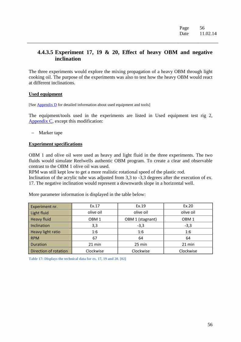
Page : 56

Date : 11.02.14

56

4.4.3.5 Experiment 17, 19 & 20, Effect of heavy OBM and negative

inclination

The three experiments would explore the mixing propagation of a heavy OBM through light

cooking oil. The purpose of the experiments was also to test how the heavy OBM would react

at different inclinations.

Used equipment



Appendix C, except this modification:

Marker tape


OBM 1 and olive oil were used as heavy and light fluid in the three experiments. The two

fluids would simulate Reelwells authentic OBM program. To create a clear and observable

contrast to the OBM 1 olive oil was used.

RPM was still kept low to get a more realistic rotational speed of the plastic rod.

Inclination of the acrylic tube was adjusted from 3,3 to -3,3 degrees after the execution of ex.

17. The negative inclination would represent a downwards slope in a horizontal well.


Experiment nr. Ex.17 Ex.19 Ex.20

Light fluid olive oil olive oil olive oil

Heavy fluid OBM 1 OBM 1 (stagnant) OBM 1

Inclination 3,3 -3,3 -3,3

Heavy light ratio 1:6 1:6 1:6

RPM 67 64 64

Duration 21 min 25 min 21 min

Direction of rotation Clockwise Clockwise Clockwise

Table 17: Displays the technical data for ex. 17, 19 and 20. [02]

Page : 57

Date : 11.02.14

57

Execution




When performing experiments 17, 19 and 20 certain irregularities may have caused


Experiment 19 was performed using a stagnant OBM 1. This may have caused

reduced mixing between the heavy and light fluid, and therefore affected the spread of

the mixing zone.

The three experiments experienced that the heavy fluid tainted the inner wall of the

acrylic tube. This resulted in that some of the OBM 1 got mixed instantly when the

test started. This may have affected the observation of the mixing zone interface.

Page : 58

Date : 11.02.14

58




Rpm Syrup 2 OBM 1 Olive oil

ϴ600 >300 45,0 151,0

ϴ300 249,0 25,0 77,0

ϴ200 167,0 18,0 52,0

ϴ100 84,0 10,0 27,0

ϴ6 6,0 3,0 3,0

ϴ3 3,5 2,0 2,0

PV (cp) >51 20,0 74,0

YP (lb/100 ft2) <198 5,0 3,0

ρ (s.g) 1,370 1,210 0,910

n 0,848 0,971

Table 18: Showing the fluid properties for the heavy and light fluids used in test rig 2#. [02]


0 100 200 300 400 500 600

0,0

50,0

100,0

150,0

200,0

250,0

300,0

Vis

cosi

ty (

lb/1

00

ft2

)

RPM


Syrup 2 Olive oil OBM 1

Graph 12: Displays the fluid rheology to the liquids used in test rig 2#. [02]

Page : 59

Date : 11.02.14

59







0,0

5,0

10,0

15,0

20,0

25,0

0,0 5,0 10,0 15,0 20,0 25,0

Len

gth

of

mix

ingz

on

e (

cm)

Time (min)

Test rig 2

Ex 14

Ex 15

Ex 17

Ex 19

Ex 20

0

4000

8000

12000

16000

20000

24000

28000

32000

36000

40000

44000

48000

65 100 200 1000

Re

yno

lds

nu

mb

er

RPM

Flow pattern, experiments conducted with Syrup 2 and (dyed) water

Re - Water

Re - Syrup 2

Re - Mixing zone

Turbulence

Transitional

Laminar

Graph 13: Illustrates the propagation of the mixing interface for all applicable experiments

conducted with test rig 2#. [02]

Chart 1: The flow pattern of test rig 2 experiments conducted with Syrup 2 and water. [02]

Page : 60

Date : 11.02.14

60

All experiments conducted with syrup and water can refer to the chart 1. It states that all syrup

water experiments with rotational speed higher than 100 RPM has turbulence in the water

phase flow. The turbulent flow may have affected the mixing zone propagation.

Experiment 8 & 9, Effect of reduced RPM


[03].

Ex. 8 High RPM

Experiment

start Time 0.00 min

Experiment

stop Time 20.00 min

Ex. 9 Reduced RPM*

Experiment

start Time 0.00 min

Experiment

stop Time 20.00 min

Screenshot tables 4: Screenshots from the experimental footage taken under the execution of experiments 8 and 9. [03]

* = Assumed to be over 100 RPM

The two experiments results were inconclusive in regard to observation of mixing zone

movement. An excess of the blackly dyed water made the heavy light interface stretch

through the entire acrylic tube in both experiments (see screenshot table 4). This made it

difficult to observe any clear movement of the heavy light interface.

As seen in tables above and in the attached experimental CD, there is a noticeable difference

between the experiment conducted with high RPM (ex. 8) and the one with reduced RPM (ex.

9).

The high RPM experiment has a distinct colour difference from the far left to the far right of

the acrylic pipe. The distribution of heavy and light liquid seems to have arranged itself after

the characteristics of the interface.

In the reduced RPM scenario, mixing zone spread is more uniform which is shown by the

similar colour scheme. This development contradicts what is suggested by the Reynolds

numbers in chart 1, where a higher rotation speed develops a more turbulent rotational flow.

Page : 61

Date : 11.02.14

61

Experiment 10, 11, 12 & 13, Effect of heavy light ratio

The four experiments results are shown using screenshots from the experimental footage [03].

Ex. 10 1:4 heavy light fluid ratio

Experiment

start Time 0.00 min

Experiment

stop Time 20.00 min


Experiment

start Time 0.00 min

Experiment

stop Time 20.00 min


Experiment

start Time 0.00 min

Experiment

stop Time 20.00 min


Experiment

start Time 0.00 min

Experiment

stop Time 20.00 min

Screenshot tables 5: Screenshots from the footage taken under the execution of experiments 10, 11, 12 and 13. [03]

Page : 62

Date : 11.02.14

62

The four experiments resulted in no viable observation of the mixing zone. The dye added to

the light fluid (ex. 10) and the heavy fluid (ex. 11, 12 and 13) overpowered the other fluids

colour.

Since all experiments were conducted with very high RPM, the fluid movement in the

experiments were in turbulence. The turbulence may have accelerated the discoloration of the

fluid system.

The black dye added to distinguish the heavy and light liquid seems to be too dominant, and

clouded any mixing interface observation. Weaker doses of black dye may simplify

observation in future experiments.

Experiment 14 & 15, Effect of Clockwise (CW) and Anticlockwise (ACW) rotation


footage [03] and graphs and tables from the Experiment sheet

[02].

Ex. 14 CW

Experiment

start Time 0.00 min

Experiment

stop Time 20.00 min

Ex. 15 ACW

Experiment

start Time 0.00 min

Experiment

stop Time 20.00 min

Screenshot tables 6: Screenshots from the experimental footage taken under the execution of experiments 14 and 15.

[03]

Page : 63

Date : 11.02.14

63

Experiment 14 and 15 showed that the plastic rods grooves have an effect on the mixing

interface propagation. The graph 14 and the screenshot table 6 displays a noticeable

difference between the experiments performed with CW and ACW rotation. The CW

experiment have a more steep mixing rate before it levels out, while the ACW has a more

linear trajectory.

This is supported by the displayed trend lines, that show that the mixing rates of the two

experiments are different (0,4145 ≠ 0,3624).

0,0

2,5

5,0

7,5

10,0

0,0 5,0 10,0 15,0 20,0

Len

gth

of

mix

ingz

on

e (

cm)

Time (min)

Test rig 2: Clockwise VS. Anticlockwise

CW

ACW

Mixing rateCW = 0,4145 cm/min

Mixing rateACW = 0,3624 cm/min

0,0

2,5

5,0

7,5

10,0

0,0 5,0 10,0 15,0 20,0

Len

gth

of

mix

ingz

on

e (

cm)

Time (min)

Test rig 2: Clockwise VS. Anticlockwise (trend lines)

CW

ACW

Graph 14: Displays the effect of CW and ACW gained from experiment 14 and 15. [02]


Page : 64

Date : 11.02.14

64

Experiment 16 & 18, Effect of low RPM

The two experiments results are displayed using screenshots from the experimental footage

[03].

Ex. 16

Experiment

start Time 0.00 min

Experiment

stop Time 20.00 min

Ex. 18

Experiment

start Time 0.00 min

Experiment

stop Time 20.00 min

Screenshot tables 7: Screenshots from experimental the footage taken under the execution of experiments 16 and 18.

[03]

As for experiments 10, 11, 12 and 13, the two tests experienced that the divisive dye scheme

failed. Displayed in the table above, the dye malfunction is clear. No observable heavy light

mixing interface was seen during experiments 16 and 18.

The low RPM had no noticeable effect on the colour contamination of the test system. The

colour distribution spread at a similar rate as in the >1000 RPM scenarios (see attached

experimental CD).

Dyed heavy fluids seem to have a negative effect on mixing zone movement observation.

Page : 65

Date : 11.02.14

65

Experiment 17, 19 & 20, Effect of heavy OBM and negative inclination



Ex. 17 OBM 1 inclination 3,3

Experiment

start Time 0.00 min

Experiment

stop Time 21.00 min

Ex. 19 Stagnant OBM 1 inclination -3,3

Experiment

start Time 0.00 min

Experiment

stop Time 25.00 min

Ex. 20 OBM 1 inclination -3,3

Experiment

start Time 0.00 min

Experiment

stop Time 21.00 min

Screenshot tables 8: Screenshots from the experimental footage taken under the execution of experiments 17, 19 and

20. [03]

The OBM 1 as heavy and the olive oil as the light fluid created a clear contrast to each other.

This simplified the observation process.

Page : 66

Date : 11.02.14

66

The three experiments showed a clear and observable mixing zone movement which is

displayed in the screenshot table 8 and graph 16.

Experiment 19 was performed with OBM 1 which had not been stirred. This resulted in

reduced mixing zone propagation.

The two other experiments showed a similar mixing interface movement. The negative

inclination seems to have a minor, but noticeable impact on the spread rate of the mixing

zone.

As seen in graph 17, the two comparable experiments have similar trend lines and mixing

rates. The trend lines show that the negative inclination has an increasing effect on the heavy

light interface movement. To explore further development, larger test parameters are needed.

0,0

5,0

10,0

15,0

20,0

25,0

0,0 5,0 10,0 15,0 20,0 25,0

Len

gth

of

mix

ingz

on

e (

cm)

Time (min)

Test rig 2: Effect of heavy OBM and negative inclination

OBM 1, Incli 3,3 OBM 1, Incli -3,3 Stagnant OBM 1, Incli -3,3

Mixing rate3,3 = 0,8580 cm/min

Mixing rate-3,3 = 1,0474 cm/min

Mixing ratestagnant,-3,3 = 0,1075 cm/min

0,0

5,0

10,0

15,0

20,0

25,0

0,0 5,0 10,0 15,0 20,0 25,0

Len

gth

of

mix

ingz

on

e (

cm)

Time (min)

Test rig 2: Effect of heavy OBM and negative inclination (trend lines)

Stagnant OBM 1, Incli -3,3 OBM 1, Incli 3,3 OBM 1, Incli -3,3

Graph 16: Displays the mixing effect of heavy OBM and negative inclination gained from

experiments 17, 19 and 20. [02]


Page : 67

Date : 11.02.14

67

The flow pattern for the three experiments shows that all the liquids are inside the laminar

range by a wide margin. This means that the mixing zone is probably not affected by the

fluids flow characteristics. Other parameters seem to govern the mixing zone behavior.


Out of all factors tested with test rig 2#, negative inclination seem to have the highest effect

on increasing the mixing zone movement (see table below). On the other hand, stagnant OBM

almost stopped heavy light interface propagation. This indicates that the rheology of the

heavy fluid has a significant effect on the mixing zone distribution.


Ex.14 CW 7,5 0,4145

Ex.15 ACW 7,5 0,3624

Ex.17 OBM, inclination 3,3 17,5 0,8580

Ex.19 Stagnant OBM, inclination -3,3 2,5 0,1075

Ex.20 OBM, inclination -3,3 22,5 1,0474




Test rig 2#s experimental setup approached Reelwells heavy over light scenario, but it lacked

size and predictability. RPM, inclination and pipe sizes are parameters that are varied under

real conditions. A new test rig should have the capability to test and vary these parameters in

experiments with longer duration and at a bigger scale.

0

50

100

150

200

250

Re

yno

lds

nu

mb

er

65 RPM

Flow pattern, experiments conducted with OBM 1 and Olive oil

Re - OBM 1

Re - Olive oil

Re - Mixing zone

Laminar

Chart 2: Shown the flow pattern of experiments conducted with OBM 1 and olive oil. [02]

Page : 68

Date : 11.02.14

68

4.5 Test rig 3 #

4.5.1 Purpose

The purpose of test rig 3# was to build on the knowledge and experience gained from the

previous experiments and rigs. The new test rig would attempt to simulate the propagation of

the mixing zone propagation in a more realistic environment. This meant that the run time of

the experiments had to be longer, the test parameters had to be bigger and fluids with more

realistic properties had to be used. The following parameters could now be tested (as well as

previously tested parameters from test rig 1 and 2):

More accurate RPM variations

Different pipe ODs

Prolonged experiment duration

Extreme inclination variations

Realistic fluid properties

With these new parameters the third test rig approached Reelwells realistic scenario, and

results gained from it would shape the heavy light mixing conclusion.

In test rig #3 the effect of clockwise and anticlockwise rotation is assumed negligible due to

the lack of lathe induced groves and other disturbances created by the aluminum pipe.

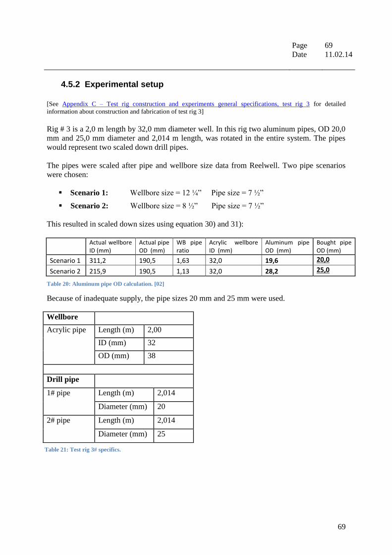
Page : 69

Date : 11.02.14

69


[See Appendix C – Test rig construction and experiments general specifications, test rig 3 for detailed

information about construction and fabrication of test rig 3]

Rig # 3 is a 2,0 m length by 32,0 mm diameter well. In this rig two aluminum pipes, OD 20,0

mm and 25,0 mm diameter and 2,014 m length, was rotated in the entire system. The pipes

would represent two scaled down drill pipes.

The pipes were scaled after pipe and wellbore size data from Reelwell. Two pipe scenarios

were chosen:

Scenario 1: Wellbore size = 12 ¼” Pipe size = 7 ½”

Scenario 2: Wellbore size = 8 ½” Pipe size = 7 ½”

This resulted in scaled down sizes using equation 30) and 31):

Actual wellbore ID (mm)

Actual pipe OD (mm)

WB pipe ratio

Acrylic wellbore ID (mm)

Aluminum pipe OD (mm)

Bought pipe OD (mm)

Scenario 1 311,2 190,5 1,63 32,0 19,6 20,0

Scenario 2 215,9 190,5 1,13 32,0 28,2 25,0

Table 20: Aluminum pipe OD calculation. [02]

Because of inadequate supply, the pipe sizes 20 mm and 25 mm were used.

Wellbore

Acrylic pipe Length (m) 2,00

ID (mm) 32

OD (mm) 38

Drill pipe

1# pipe Length (m) 2,014

Diameter (mm) 20

2# pipe Length (m) 2,014

Diameter (mm) 25

Table 21: Test rig 3# specifics.

Page : 70

Date : 11.02.14

70

Picture 3: Test rig 3 # setup with used equipment positioned for a test of feasibility of future experiments. The acrylic pipe

displayed has an inclination of 2,0o relative to the horizontal plane. The 20 mm diameter aluminum pipe is mounded

through the sponge plug into the drill. The drill are fitted with different tensioned plastic strips Weights are placed on

both stands to ensure stability, while the workshop stand holds the heavy end in angle. [01]

Page : 71

Date : 11.02.14

71


4.5.3.1 Experiment 21, 22, 23 and 24, Effect of RPM and pipe size,

Matrix 1

The purpose of the four experiments was to map how different RPM and pipe sizes effect the

spread of the mixing zone. A secondary objective was to test the rigs durability and stability.

Battery life of the camera and the drill were also tested.

Used equipment



Appendix C.

No modification to that list was used in these experiments.


All four experiments used canola oil as the light liquid and OBM 2 as the heavy liquid.

Canola oil was chosen because of its transparency. The feature would highlight the travel of

the heavy fluid interfaces up through the acrylic pipe.

RPM and pipe size was varied from experiment to experiment to learn how the two

parameters influence the mixing zone movement.

Inclination was put at 2,0 degrees to simulate more realistic conditions. The test rig was not

positioned at Reelwells 1,0 degrees because of concerns about the spread of the heavy light

interface.



Light fluid canola oil canola oil canola oil canola oil

Heavy fluid OBM 2 OBM 2 OBM 2 OBM 2



Pipe OD (mm) 20 20 25 25

RPM 60 150 60 150




Page : 72

Date : 11.02.14

72

Execution




When performing experiments 21, 22, 23 and 24 certain irregularities may have caused

unplanned events. Listed are the events that were discovered:

Experiment 23 was performed without using the plastic hose to fill the acrylic tube

with heavy fluid. The event made it impossible to observe the mixing zone

distribution.

Page : 73

Date : 11.02.14

73

4.5.3.2 Experiment 25, Effect of low viscous light fluid

Experiment 25s main objective was to test the effect of a low viscous light fluid had on the

expansion of the mixing zone interface. The experiment would also represent worst case

scenario when it came mixing between a heavy and light oil-based liquid.

Used equipment



Appendix C.



The experiment used gasoline grade diesel as light liquid and the OBM 2 as heavy. Diesel

was used for its viscous abilities which would create a strong contrast to the canola oil used in

the previous experiments. The diesel is also a clear fluid, which would simplify interface

observation.

Inclination was kept at 2,0 degrees.


Experiment nr. Ex.25

Light fluid diesel

Heavy fluid OBM 2

Inclination 2,0

Heavy light ratio 1:4

Pipe OD (mm) 20

RPM 60

Duration 60 min

Direction of rotation Clockwise

Table 23: Displays the technical data for ex. 25. [02]

Execution

[Experiment 25 followed the same procedure and execution]



No specific uncertainties were detected.

Page : 74

Date : 11.02.14

74

4.5.3.3 Experiment 26, 27, 28 and 29, Effect of RPM and pipe size,

Matrix 2

The four experiments main objective was to build on experience gained from previous test rig

3# experiments. RPM and pipe sizes mixing effect would be tested in these experiments.

Used equipment



Appendix C.



Experiments 26, 27, 28 and 29 used diesel + rapeseed oil as light fluid while OBM 2 were

used as heavy fluid. The diesel + rapeseed light liquid was used to create a more similar fluid

system relative to Reelwells OBM program.

Inclination was kept at 2,0 degrees.



Light fluid diesel + rapeseed oil diesel + rapeseed oil diesel + rapeseed oil diesel + rapeseed oil

Heavy fluid OBM 2 OBM 2 OBM 2 OBM 2



Pipe OD (mm) 20 20 25 25

RPM 60 150 60 150




Execution





Page : 75

Date : 11.02.14

75

4.5.3.4 Experiment 30 and 31, Effect of negative inclination

Experiment 30 and 31 would explore the effect of negative inclination and distinguish

between mixing in a positive and negative tilt.

Used equipment



Appendix C.



Both experiments had the same fluid configuration as experiments 26, 27, 28 and 29 except

for the utilization of OBM 3 instead of OBM 2. Test 30 had a negative inclination of -2,0

degrees to simulate a downwards slope in a horizontally planned wellbore.

Experiment 31 was done as a technical exercise, with an unlikely inclination of -90,0 degrees.



Light fluid diesel + rapeseed oil diesel + rapeseed oil

Heavy fluid OBM 3 OBM 3

Inclination -2,0 -90,0


Pipe OD (mm) 20 25

RPM 60 150




Execution





Page : 76

Date : 11.02.14

76




Rpm OBM 2 OBM 3 Canola oil* Rapeseed oil* Diesel Diesel + Rapeseed oil

ϴ600 46,0 44,0 133,0 133,0 8,0 41,5

ϴ300 26,0 24,0 68,0 68,0 4,0 21,5

ϴ200 17,0 16,0 46,0 46,0 3,0 14,5

ϴ100 10,0 9,0 24,0 24,0 2,0 7,5

ϴ6 3,0 2,5 2,0 2,0 1,0 1,5

ϴ3 2,0 1,5 1,0 1,0 0,5 1,0

PV (cp) 20,0 20,0 65,0 65,0 4,0 20,0

YP (lb/100 ft2) 6,0 4,0 3,0 3,0 0,0 1,5

ρ (s.g) 1,215 1,200 0,915 0,915 0,845 0,885

n 0,823 0,874 0,967 0,967 0,999 0,948


* = Canola and Rapeseed are the same oil type. Both are displayed because of the use of both terms in thesis.

0 100 200 300 400 500 600

0,0

20,0

40,0

60,0

80,0

100,0

120,0

140,0

Vis

cosi

ty (

lb/1

00

ft2

)

RPM


OBM 2 OBM 3 Canola oil Diesel Diesel + Rapeseed oil Rapeseed oil


Page : 77

Date : 11.02.14

77

As shown in Drilling fluid preparation and description OBM 1, 2 and 3 have the same recipe.

Irregularities in rheology illustrated in graph 19 are due to errors committed when creating the

fluids as well as uncertainties in measurement equipment.

The irregularities are assumed negligible with regard to comparing experiments performed

with the heavy liquid.







0,0

10,0

20,0

30,0

40,0

50,0

60,0

70,0

80,0

90,0

100,0

0,0 10,0 20,0 30,0 40,0 50,0 60,0

Len

gth

of

mix

ingz

on

e (

cm)

Time (min)

Test rig 3

Ex 21

Ex 22

Ex 24

Ex 25

Ex 26

Ex 27

Ex 28

Ex 29

Ex 30

0 100 200 300 400 500 600

0,0

10,0

20,0

30,0

40,0

50,0

Vis

cosi

ty (

lb/1

00

ft2

)

RPM

Fluid rheology OBM 1, 2 and 3

OBM 1 OBM 3 OBM 2


Graph 19: Displays the fluid rheology to OBM 1, 2 and 3. [02]

Page : 78

Date : 11.02.14

78

Experiment 21, 22, 23 and 24, Effect of RPM and pipe size



Ex. 21 RPM 60 Pipe size 20 mm

Experiment

start Time 0.00 min

Experiment

stop Time 60.00 min


Experiment

start Time 0.00 min

Experiment

stop Time 60.00 min

Ex. 23* RPM 60 Pipe size 25 mm

Experiment

start Time 0.00 min

Experiment

stop Time 60.00 min


Experiment

start Time 0.00 min

Experiment

stop Time 60.00 min

Screenshot tables 9: Screenshots from ex. footage taken under the execution of experiments 21, 22, 23 and 24. The

bended illustration of some of the experiments is due to a fish eyed lens, not experiment setup. [03]

Page : 79

Date : 11.02.14

79

* Experiment 23 was too contaminated to give

an observable result. The experiment was

not repeated because of OBM shortage and

future experiments would repeat the tests

major specifics (see ex. 28).

= Highest interface movement

= intermediate interface movement

= Lowest interface movement

As displayed in the tables and graphs above, mixing zone propagation increases with lower

RPM and smaller pipe sizes. When subjected to decreasing force of friction from the rotating

body, the fluids seem to need longer time to stabilize a constant mixing rate. This event is

especially noticeable in experiment 21, where it takes almost 10 minutes before a consistent,

decreasing mixing rate is established.

Matrix nr. 1 RPM

60 150

Pipe size

(mm)

20 Ex 21 Ex 22

25 Ex 23* Ex 24

Table 27: Displays matrix nr. 1.

0,0

10,0

20,0

30,0

40,0

0,0 10,0 20,0 30,0 40,0 50,0 60,0

Len

gth

of

mix

ingz

on

e (

cm)

Time (min)

Test rig 3: Effect of RPM and pipe size (trend lines)

RPM 60, Pipe size 20 RPM 150, Pipe size 20 RPM 150, Pipe size 25

0,0

5,0

10,0

15,0

20,0

25,0

30,0

35,0

40,0

0,0 10,0 20,0 30,0 40,0 50,0 60,0

Len

gth

of

mix

ingz

on

e (

cm)

Time (min)

Test rig 3: Effect of RPM and pipe size, matrix 1

RPM 60, Pipe size 20 RPM 150, Pipe size 20 RPM 150, Pipe size 25

Graph 21: Displays the mixing effect of RPM and pipe size gained from experiments 21, 22, 23 and 24. [02]


Page : 80

Date : 11.02.14

80

RPM and pipe size Trend line equation



60, 20 mm y = 0,6248x + 8,6946 36 0,6248

150, 20 mm y = 0,1849x + 1,0191 6 0,1849

60, 25 mm VOID VOID VOID

150, 25 mm y = 0,0682x + 0,0581 4 0,0682

Table 28: Displays the mixing zone movement results from ex. 21, 22, 23 and 24. [02]



Trend lines, mixing distances and mixing rates displayed in graph 22 and table 28 also

suggest an increase in heavy light interface movement at small pipe size and low RPM.

The table above shows also that the highest mixing rate is relatively low when compared to

experiments conducted with OBM and oil in test rig 2. This may be due to the high viscosity

of the Canola/Rapeseed oil, which may be reducing the mixing interfaces movement. To see

the clear effect of light fluid viscosity, an experiment conducted with a low viscous light fluid

should be performed.

The test matrix 1s flow pattern partly backs up the observed mixing movement in screenshot

tables and graphs. Even if all Reynolds numbers are in the laminar range, as seen in the chart,

the Re-numbers for pipe size 1# is higher than the ones for pipe size 2#.

What doesn’t correlate with the flow pattern is that we don’t observe an increase in mixing

zone movement at higher RPM. Since all the Re-numbers are in the laminar range, the flow

characteristics effect may be governed by other parameters.

0

200

400

600

800

1000

1200

60 150

Re

yno

lds

nu

mb

er

RPM

Flow pattern, test matrix 1

Re 1# - OBM 2

Re 1# - Canola oil

Re 1# - Mixing zone

Re 2# - OBM 2

Re 2# - Canola oil

Re 2# - Mixing zone

Laminar

Chart 3: The flow pattern for experiments conducted according to Matrix 1. [02]

1# = Small pipe size (20 mm)

2# = Large pipe size (25 mm)

Page : 81

Date : 11.02.14

81

Experiment 25, Effect of low viscous light fluid



Ex. 25

Experiment

start Time 0.00 min

Before

camera angle

movement Time 28.00 min

After camera

angle


Experiment

stop Time 60.00 min

Screenshot tables 10: Screenshots from ex. footage taken under the execution of experiment 25. The bended

illustration of some of the experiments screenshots are due to a fish eyed lens, not experiment setup. [03]

0,0

20,0

40,0

60,0

80,0

100,0

120,0

0,0 10,0 20,0 30,0 40,0 50,0 60,0

Len

gth

of

mix

ingz

on

e (

cm)

Time (min)

Test rig 3: Effect of low viscous light fluid

Ex 25

Trend line


Page : 82

Date : 11.02.14

82

As seen in tables 29 and graph 23 the mixing propagation is extensive, and reaches almost a

meter an hour. The low viscous diesel shows a low resistance against mixing and allows the

OBM 2 to travel through in a slowly decreasing rate. The experiment represents a worst case

scenario when it comes to the effect of low viscosity in the light liquid.

As previously seen in ex. 21 the mixing rate needs time to stabilize. Graph 23 shows a mixing

surge in the beginning of the experiment, before the graph evens out and decreases at a stable

rate. The shape of the graph suggests that the mixing interface movement will stop at some

point.

The flow pattern for the experiment is inside the laminar area, but as seen in the chart above,

the Reynolds Number of the light fluid (diesel) is approaching transitional flow. The elevated

Re-number of the diesel may have been a leading factor in increasing the mixing zone

movement.




60, 20 mm y = 1,4274x + 20,965 86 1,4274

Table 29: Displays the mixing zone movement result from ex. 25. [02]

0

500

1000

1500

2000

60

Re

yno

lds

nu

mb

er

RPM

Flow pattern, Ex. 25

Re 1# - Diesel

Re 1# - OBM 2

Re 1# - Mixing zone

Laminar

Transitional

Chart 4: Displays the flow pattern of experiment 25. [02]

Page : 83

Date : 11.02.14

83

Experiment 26, 27, 28 and 29, Effect of RPM and pipe size




Experiment

start Time 0.00 min

Experiment

stop Time 60.00 min


Experiment

start Time 0.00 min

Experiment

stop Time 60.00 min


Experiment

start Time 0.00 min

Experiment

stop Time 60.00 min


Experiment

start Time 0.00 min

Experiment

stop Time 60.00 min

Screenshot tables 11: Screenshots from ex. footage taken under the execution of experiments 26, 27, 28 and 29. The

bended illustrations of some of the experiments are due to a fish eyed lens, not experiment setup. [03]

Page : 84

Date : 11.02.14

84

= Highest interface movement

= intermediate interface movement

= Lowest interface movement

Matrix nr. 2 RPM

60 150

Pipe size

(mm)

20 Ex 26 Ex 27

25 Ex 28 Ex 29

Table 30: Displays matrix nr. 2.

0,0

10,0

20,0

30,0

40,0

50,0

0,0 10,0 20,0 30,0 40,0 50,0 60,0

Len

gth

of

mix

ingz

on

e (

cm)

Time (min)

Test rig 3: Effect of RPM and pipe size, Matrix 2

OD 20, RPM 60 OD 20, RPM 150 OD 25, RPM 60 OD 25, RPM 150

0,0

10,0

20,0

30,0

40,0

50,0

60,0

0,0 10,0 20,0 30,0 40,0 50,0 60,0

Len

gth

of

mix

ingz

on

e (

cm)

Time (min)

Test rig 3: Effect of RPM and pipe size, Matrix 2, (trend lines)

RPM 60, OD 20 RPM 150, OD 20 RPM 60, OD 25 RPM 150, OD 25



Page : 85

Date : 11.02.14

85




60, 20 mm y = 0,8187x + 11,248 50 0,8187

150, 20 mm y = 0,3652x + 10,648 28 0,3652

60, 25 mm y = 0,1512x + 2,0725 10 0,1512

150, 25 mm y = 0,357x + 3,7203 16 0,3570

Table 31: Displays the mixing zone movement results from ex. 26, 27, 28 and 29. [02]



As shown in the tables and graphs above, mixing zone propagation and mixing rate increases

with lower RPM and smaller pipe sizes. As seen in previous experiments 21, 22 and 25

decreasing force of friction from the rotating body fail to keep the fluid in suspense from the

start. It takes longer time to stabilize the fluids to flow at a constant mixing rate. Experiment

27 seen in graph 24 show an extreme case of the phenomenon. The high RPM fails in rotating

the heavy fluid and it travels up the tube at a rapid rate, before it stabilizes together with the

light liquid and continues at a severely reduced mixing rate.

The experiments conducted with large pipe size show a different graph movement. A clear

heavy light interface gets created almost instantly after start (see attached experimental CD)

and moves at a predictable and stable rate. The two experiments performed with the large pipe

size has both these traits, but unexpectedly the high RPM experiment has a higher mixing rate

and mixing distance than the experiment with a low RPM.

One explanation for the high mixing zone movement in the “RPM 150, 25 mm” experiment

could be that the high RPM and large pipe size creates turbulent flow, which then again

accelerates mixing. As seen in chart 5 below, this is not the case, but there seems to be a

“sweet spot” where a fixed RPM and pipe size results in minimal heavy light interface

propagation. As seen in table 14, the “sweet spot” seems to lie in the proximity of 60 RPM

and 25 mm pipe size for this test setup.

The four experiments results indicate that high RPM and the large pipe size seems to stabilize

the liquid faster and initiates a more horizontal slope than seen in experiments conducted with

low RPM and small pipe size.

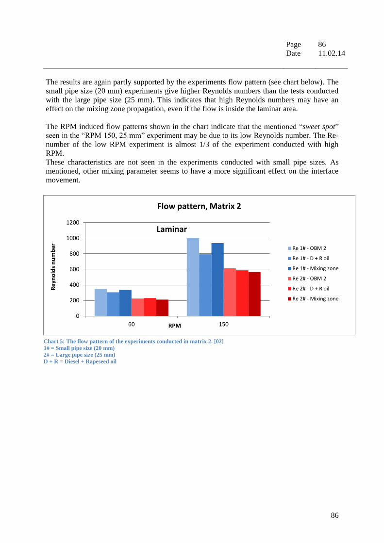
Page : 86

Date : 11.02.14

86

The results are again partly supported by the experiments flow pattern (see chart below). The

small pipe size (20 mm) experiments give higher Reynolds numbers than the tests conducted

with the large pipe size (25 mm). This indicates that high Reynolds numbers may have an

effect on the mixing zone propagation, even if the flow is inside the laminar area.

The RPM induced flow patterns shown in the chart indicate that the mentioned “sweet spot”

seen in the “RPM 150, 25 mm” experiment may be due to its low Reynolds number. The Re-

number of the low RPM experiment is almost 1/3 of the experiment conducted with high

RPM.

These characteristics are not seen in the experiments conducted with small pipe sizes. As

mentioned, other mixing parameter seems to have a more significant effect on the interface

movement.

0

200

400

600

800

1000

1200

60 150

Re

yno

lds

nu

mb

er

RPM

Flow pattern, Matrix 2

Re 1# - OBM 2

Re 1# - D + R oil

Re 1# - Mixing zone

Re 2# - OBM 2

Re 2# - D + R oil

Re 2# - Mixing zone

Laminar

Chart 5: The flow pattern of the experiments conducted in matrix 2. [02]



D + R = Diesel + Rapeseed oil

Page : 87

Date : 11.02.14

87

Experiment 30 and 31, Effect of negative inclination



Ex. 30 Inclination -2,0

Experiment

start Time 0.00 min

Before

camera angle


After camera

angle


Experiment

stop Time 60.00 min

Screenshot tables 12:

Screenshots from ex.

footage taken under the

execution of experiments

30 and 31. Screenshots

from experiment 31 is

taken two different

cameras. The second

camera took over when

the mixing zone had

moved past the range of

the lens. As seen in the

top of the third

screenshot from the left,

the mixing zone is

moving downwards.

The bended illustration

of some of the

experiments is due to a

fish eyed lens, not

experiment setup. [03]

Ex.

info

Experiment start

Time 0.00 min

Before camera change

Time 5.00 min

Before camera change

Time 5.00 min

Experiment stop

time 20.00 min

31#

-90,0o

Page : 88

Date : 11.02.14

88

The screenshot tables and the graphs above show that negative inclination has a profound

effect on the mixing zone propagation. As partly shown in experiment 20 from test rig 2#, the

negative inclination seem to form a linear mixing rate after stabilizing the fluid rotation. This

can especially be seen in experiment 30 (inclination -2,0), where the graph seems to follow a

linear trend after a stabilizing process lasting 20 minutes.

0,0

20,0

40,0

60,0

80,0

100,0

120,0

0,0 10,0 20,0 30,0 40,0 50,0 60,0

Len

gth

of

mix

ingz

on

e (

cm)

Time (min)

Test rig 3: Effect of negative inclination

-2,0 degrees

-90,0 degrees

0,0

20,0

40,0

60,0

80,0

100,0

120,0

0,0 10,0 20,0 30,0 40,0 50,0 60,0

Len

gth

of

mix

ingz

on

e (

cm)

Time (min)

Test rig 3: Effect of negative inclination (trend lines)

-2,0 degrees

-90,0 degrees

Graph 26: Displays the mixing effect of negative inclination gained from experiments 30 and 31. [02]


Page : 89

Date : 11.02.14

89

Table 32: Displays the mixing zone movement results from ex. 30 and 31. [02]

* = Experiment 31 was only run 20 minutes. Mixing distance would have been larger if test parameters would have

allowed. Increased mixing distance (%) could not be calculated because of lack of test parameters.

The mixing distance and rate of the two experiments seem to confirm the negative

inclinations effect. As displayed in table 32 the mixing rate increases with 1357,4 % from

negative inclination of -2,0 to -90,0. The high RPM and large pipe size did not seem to slow

down the mixing interface movement in any usable manner. As seen in the attached

experimental CD, the heavy fluid manages to stick into the wall and escape the movement of

the rotating pipe. When the heavy fluid gets picked up by the force of rotation, the heavy light

interface has moved considerably farther down the tube. These surges can easily be seen in

graph 28. The graph also show the periods of less mixing that comes after these surges.

The linear shape of the two negative inclination graphs suggest that if the experiments had

continued, the mixing zone movement would have kept its present mixing rate until the space

had run out. It seems like the constant force of gravity governs the mixing rate for

experiments conducted with negative inclination, and sets a constant mixing rate. If that is so,

prediction of the mixing rate may be possible.

Inclination Trend line equation Mixing distance (cm)


Increased mixing distance (%)

Increased mixing rate (%)

-2,0 y = 1,0595x + 10,716 70 1,0595 VOID 0

-90,0 y = 14,382x + 9,9664 124* 14,382 VOID 1357,4

0,0

20,0

40,0

60,0

80,0

100,0

120,0

140,0

0,0 2,0 4,0 6,0 8,0 10,0

Len

gth

of

mix

ingz

on

e (

cm)

Time (min)

Experiment 31, Areas of surge and reduced mixing

Graph 28: Displays the areas of surge and reduced mixing in experiment 31. [02]

Page : 90

Date : 11.02.14

90

The two experiments are conducted with virtually the same fluid configuration as used in

Matrix 2 (ex. 26, 27, 28 and 29), with the only difference being the usage of OBM 3 instead

of OBM 2. The flow pattern has therefore a similar flow characteristic as Matrix 2

experiments, and is in the laminar area. Because of the extreme difference in inclination

between the experiments, the effect of Reynolds number difference is obscured.

0

100

200

300

400

500

600

700

60 150

Re

yno

lds

nu

mb

er

RPM

Flow pattern, Ex. 30 and 31

Re 1# - OBM 3

Re 1# - D + R oil

Re 1# - Mixing zone

Re 2# - OBM 3

Re 2# - D + R oil

Re 2# - Mixing zone

Laminar

Chart 6: The flow pattern of experiments 30 and 31. [02]



D + R = Diesel + Rapeseed oil

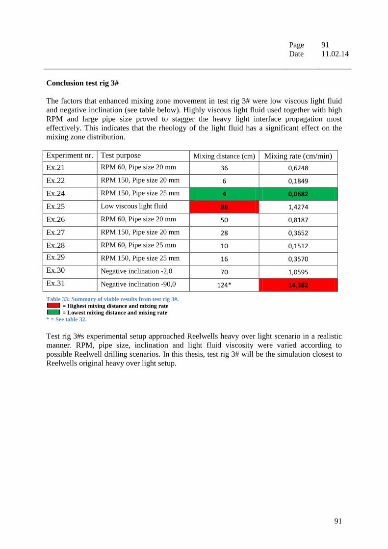
Page : 91

Date : 11.02.14

91


The factors that enhanced mixing zone movement in test rig 3# were low viscous light fluid

and negative inclination (see table below). Highly viscous light fluid used together with high

RPM and large pipe size proved to stagger the heavy light interface propagation most

effectively. This indicates that the rheology of the light fluid has a significant effect on the

mixing zone distribution.


Ex.21 RPM 60, Pipe size 20 mm 36 0,6248



Ex.25 Low viscous light fluid 86 1,4274





Ex.30 Negative inclination -2,0 70 1,0595

Ex.31 Negative inclination -90,0 124* 14,382




* = See table 32.

Test rig 3#s experimental setup approached Reelwells heavy over light scenario in a realistic

manner. RPM, pipe size, inclination and light fluid viscosity were varied according to

possible Reelwell drilling scenarios. In this thesis, test rig 3# will be the simulation closest to

Reelwells original heavy over light setup.

Page : 92

Date : 11.02.14

92

4.6 Viscometer test rig

4.6.1 Purpose

The Viscometer test rigs purpose was to explore the effect of varying RPM on mixing zone

movement in a vertical scenario. This would give a clear representation in how turbulence

from rotating objects affects heavy light interface propagation.


[See Appendix C – Test rig construction and experiments general specifications, viscometer test rig for detailed

information about construction and fabrication of viscometer test rig]

Viscometer rig is a 100 mm length by 56,3 mm diameter well (measured in accordance to

fluid level). In this rig a viscometer steel cylinder, 40,7 mm diameter and 60 mm length, was

rotated in the middle of the system 40 mm above the plastic cup bottom. It would represent

the drill pipe in a drilling scenario.

Wellbore

Plastic cup Length (mm) 100

ID (mm) 56,3

Drill pipe

Viscometer

steel cylinder

Length (mm) 60

Diameter (mm) 40,7

Table 34: Viscometer test rig specifics.

Picture 4: Viscometer test rig setup. The

plastic cup is displayed positioned onto the

Viscometers steel cylinder, filled with fluids

form the first experiment. The scale to the left

is placed to simplify the observation of the

mixing zone movement. [01]

Page : 93

Date : 01.05.14

93

4.6.1 Viscometer experiment 1 and 2

The purpose of the two experiments was to see how the heavy light interface would behave

when subjected to quantified RPM. The first experiment would explore the light fluids travel

through the heavy, while the second would investigate the heavy liquids mixing with the light.

Used equipment


The equipment/tools used in the two experiments are listed in Used equipment viscometer test

rig, Appendix C, except for this modification:

Food dye (black)


The first experiment used syrup 1 as heavy fluid and black dyed water as light fluid. The two

water based liquids would create a contrast which simplifies the observation of the light fluids

travel. The second experiment used OBM 1 as heavy fluid and olive oil as light fluid. These

two fluids had the same fluid purpose as for viscometer ex. 1, just with regard to the heavy

liquid.


Experiment Viscometer ex. 1 Viscometer ex. 2

Light fluid water + strong dye Olive oil

Heavy fluid syrup 1 OBM 1

Inclination 90 90


RPM 3, 6, 100, 200 3, 6, 100, 200

Duration 5.42 min 14.33 min


Table 35: Displays the technical data for viscometer ex. 1 and 2. [02]

Execution

[Viscometer experiments 1 and 2 followed the same procedure and execution]

The execution procedure listed in Experiment execution test rig 3 in Appendix C.



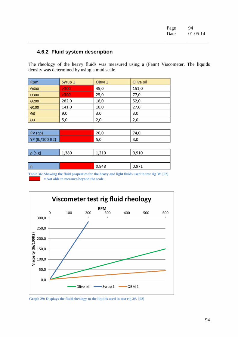
Page : 94

Date : 01.05.14

94




Rpm Syrup 1 OBM 1 Olive oil

ϴ600 >300 45,0 151,0

ϴ300 >300 25,0 77,0

ϴ200 282,0 18,0 52,0

ϴ100 141,0 10,0 27,0

ϴ6 9,0 3,0 3,0

ϴ3 5,0 2,0 2,0

PV (cp) 20,0 74,0

YP (lb/100 ft2) 5,0 3,0

ρ (s.g) 1,380 1,210 0,910

n 0,848 0,971



0 100 200 300 400 500 600

0,0

50,0

100,0

150,0

200,0

250,0

300,0

Vis

cosi

ty (

lb/1

00

ft2

)

RPM

Viscometer test rig fluid rheology

Olive oil Syrup 1 OBM 1


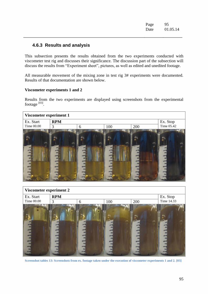
Page : 95

Date : 01.05.14

95


This subsection presents the results obtained from the two experiments conducted with

viscometer test rig and discusses their significance. The discussion part of the subsection will

discuss the results from “Experiment sheet”, pictures, as well as edited and unedited footage.


Results of that documentation are shown below.

Viscometer experiments 1 and 2

Results from the two experiments are displayed using screenshots from the experimental

footage [03]

.

Viscometer experiment 1

Ex. Start Time 00.00

RPM Ex. Stop Time 05.42 3 6 100 200

Viscometer experiment 2

Ex. Start Time 00.00

RPM Ex. Stop Time 14.33 3 6 100 200

Screenshot tables 13: Screenshots from ex. footage taken under the execution of viscometer experiments 1 and 2. [03]

Page : 96

Date : 01.05.14

96

As seen in screenshot tables 14 both experiments show that the most intensive mixing

happens at 200 RPM. At this rotational speed waves form in the heavy light interface. After a

while these waves break out and form new interfaces. This process continues until the fluids

in the plastic cup are completely mixed. This indicated that high RPM enhances mixing, and

suggest that it is recommended to stay under 200 RPM to avoid extensive mixing (in this

wellbore/drill pipe ratio scenario).

At lower RPM the interface seems unaffected and stable. 100 RPM showed some minor

indications of disturbances in the heavy light interface, but they are incomparable to mixing

propagation shown at 200 RPM. It can therefore be assumed that low RPM alone does not

enhance the mixing interface movement.

As seen in chart 7, the assumptions drawn from the screenshots seem to be supported by the

calculated Reynolds numbers from viscometer experiment 2 .Viscometer experiment 1s

Reynolds numbers couldn’t be calculated because of syrup 1s rheology.

No significant mixing was observed under 3, 6 and 100 RPM, which suggest that a laminar

flow characteristic may not have an impact on the heavy light interface movement.

At 100 RPM, some activity was seen in the test system, but this may be due to the OBM 1s

Reynolds number approaching transitional flow.

As mentioned, no accelerated mixing started before rotation speed was up to 200 RPM. The

graph above shows that interfaces movement may have been caused by the OBM 1s flow

nearly entering a turbulent pattern. As shown in the screenshot tables, the OBM mixes into

the olive oil, which complies with the data given by the chart for 200 RPM. It illustrates that it

is only the OBM 1s Re-number which enters transitional flow.

High transitional/turbulent flow seems to have a profound effect on the distribution of the

mixing zone.

0

500

1000

1500

2000

2500

3000

3500

4000

4500

3 6 100 200

Re

yno

lds

nu

mb

er

RPM

Flow pattern, viscosimeter experiment 2

Re - OBM 1

Re - Olive oil

Re - Mixing zone

Turbulent

Laminar

Transitional

Chart 7: Viscometer experiment 2s flow pattern. [02]

Page : 97

Date : 01.05.14

97

5 Discussion

In this section, results from all three test rigs will be summarized and scaled up to realistic

sizes. This will be done to clarify each parameters potential effect on heavy light interface

movement in a realistic scale. The importance and impact of these parameters will also be

discussed.

Two Reelwell WB and pipe scenarios are used to give a clear representation of the different

parameters effect on the mixing zone in real size. This will simplify the process of predicting

the interface movement.

The scenarios are the same that were scaled down for construction of test rig 3 (see section §

4.5.2 Experimental setup, test rig 3).

Reelwell scenarios Scenario 1# Scenario 2#

Meters Inch Meters Inch

Wellbore diameter 0,31 12,25 0,22 8,5

Drill pipe diameter 0,19 7,5 0,19 7,5

Table 37: Displays the two Reelwell scenarios wellbore and drill pipe diameter. [R05]

The two scenarios depend on parameter information given by Reelwell:

Range

Inclination 1o

RPM 20 - 200

ROP (m/h) 5 - 10

Table 38: Parameter information. [R05]

And the fluid configuration:

Mud type SG PPG PV YP

[kg/l] [cP] [lbs/100ft²]

Heavy OBM 1.40 11.7 30 20

Light OBM 1.10 9.2 20 20

Table 39: Reelwell fluid configuration. [R05]

These data will be used as a reference for the discussion.

Page : 98

Date : 01.05.14

98

Density difference

Density difference is an essential parameter in Reelwells heavy light concept. The difference

in density between the two fluids keeps them separated and creates the heavy light interface.

Throughout the experiments conducted with the 3 main test rigs and the viscometer rig, the

density difference between the heavy and light liquid has been varied, but only to a small

degree. Because variations in the fluid rheology occur when heavy particles are added or

removed, it was difficult to interpret the interface movement results as a product of the change

in rheology or the density.

Since density is a single parameter and rheology has a more complex composition, the fluid

densities were held in the proximity of Reelwells fluid setup. The effect of varying density

differences on interface was therefore not extensively investigated. According to the theory of

gravity, it can be assumed that an increase in density difference will slow down mixing zone

propagation. To test this assumption, fluids with similar rheological properties but different

densities should be tested in the heavy light scenario. This would illustrate the true effect of

density difference. Because of the mentioned difficulties, these investigations were not

performed in this thesis.

Information from Reelwell suggests that the concept is still under development, and that no

fixed heavy light density configuration has yet been decided.

Inclination

The parameter inclination is a leading factor in the heavy light concept, since it governs the

length of the mixing interface (in stagnant position) and the magnitude of gravity’s effect on

the system. Using the parameter information given by Reelwell together with data from

scenario 1 and 2, two potential mixing lengths can be calculated. Equation 24 is used:

Scenario (m) Calculation, equation 24 (m)

1

1o

0,31 17,75

2 0,22 12,60

Table 40: Showing the calculation of scenario 1 and 2s mixing zone lengths.

Since no axial force is affecting the test system other than gravity, no axial movement of the

two fluids should occur. If that is the case, the mixing zone length for the two scenarios will

not be longer than indicated in table 40.

Page : 99

Date : 01.05.14

99

Test rig (m) Calculation (m)

3 2o

0,032 0,912

Table 41: Showing the calculation of scenario 1 and 2s mixing zone length.

When performing the same calculations on test rig 3s wellbore (displayed in table above), in a

2 degree inclination, expected maximum mixing zone length is 0,912 m. When comparing

this length with the mixing distances derived from experiments conducted with test rig 3, it is

we observe that none of the experiments have a longer mixing zone spread. As shown in the

table below, experiment 25 has the mixing distance that approaches the to the

highest degree.

Experiment nr. Mixing distance (m)

Ex.21 0,36

Ex.22 0,06

Ex.24 0,04

Ex.25 0,86

Ex.26 0,50

Ex.27 0,28

Ex.28 0,10

Ex.29 0,16

Table 42: Displaying various experiments

mixing distances.

This experiment is a worst case scenario (see Experiment 25, Effect of low viscous light fluid)

and will therefore represent the longest mixing distance recorded with the given inclination.

Since the worst case scenario has not reached the expected mixing zone length and all

experiments conducted with positive inclination have a declining mixing slope, it can be

assumed that mixing zone length will not be significantly longer than the expected .

Because of the limited duration of the experiments (longest: 60 min) it is likely that some of

the tests would experience longer interface distances if they were run for an extended time.

However the decreasing mixing rate of the interface movement would render the extra

distance gained meaningless. This event seems to be applicable for all experiments conducted with positive inclination.

For negative inclination, interface movement has a different characteristic.

Page : 100

Date : 01.05.14

100

As seen in the graph 30, the two lines begin quite similarly, but after a while the +inclination

line decreases mixing rate and seems to evolve in a horizontal direction. After the

stabilization of the two fluids and the interface, the –inclination line continues in a positive

linear slope.

The linear slope indicates that the force of gravity and the rotational force lie in equilibrium,

with gravity trying to pull the heavy fluid downwards while the force of rotation maintains a

stable interface. This is clearly shown in attached experimental CD, Experiment 30, where the

heavy light interface moves at a steady speed down the acrylic pipe. This linear slope is also

seen in Experiment 31, where an extreme inclination of -90 degrees is held.

Summarizing the discussion and the experimental data above; wellbores with a positive

inclination will not experience significantly longer mixing zone lengths than the

calculated .

Wellbores with negative inclination will, after the fluid stabilization process, see a linear

mixing slope which directly correlates with the negative WB inclination i.e. higher negative

inclination will have an increased stable mixing rate, while a lower negative inclination will

have a decreased stable mixing rate.

0,0

10,0

20,0

30,0

40,0

50,0

60,0

70,0

80,0

0,0 10,0 20,0 30,0 40,0 50,0 60,0

Len

gth

of

mix

ingz

on

e (

cm)

Time (min)

Test rig 3: Effect of inclination

2,0 degrees

-2,0 degrees

Graph 30: Displays the mixing slopes of experiments conducted with positive and negative inclination. [02]

All other parameters than the inclination is held constant.

Page : 101

Date : 01.05.14

101

Pipe size

Varying pipe size is an important parameter in the heavy light concept. It affects the amount

of liquid inside and outside of the drill pipe, which again affects the buoyancy factor of the

pipe. Fluid rotational velocity is also dependent on the pipe size, together with RPM.

Large and small pipe sizes seem to have distinct differences in how they influence the two

fluids:

A larger pipe size exposes the external fluid for more surface friction and will thereby

have a large effect on the overall fluid velocity. An increased pipe diameter will

strengthen the rotational force on the liquids (as seen in Experiment 31).

The reduced ratio between wellbore and pipe also has a decreasing effect on the flow’s

Reynolds number. This means that drilling scenarios performed with large pipe sizes

are more likely to operate in a laminar rotational flow.

A small pipe size has a limited surface area and therefore a limited pull on the system

fluids. The pipes surface friction is not able to affect the entire fluid volume and

therefore has difficulties in creating stable rotational fluid velocity.

Small pipe sizes have the tendency to struggle with stabilizing the heavy and light

fluid at low inclinations. The interface manages to “sneak” (especially at low RPM)

under the rotating pipe and travel at a high rate before being picked up by the pipes

force of rotation. This is characterized by a mixing surge (see graph 31).

In contradiction to large pipe sizes, pipes with limited diameters increases the

Reynolds number of the flow. This may throw the rotational flow into a transitional or

turbulent flow pattern.

As seen in graph 31 and chart 8 (next page), these characteristics seem to be supported by the

experimental data.

0,0

5,0

10,0

15,0

20,0

25,0

30,0

0,0 10,0 20,0 30,0 40,0 50,0 60,0

Len

gth

of

mix

ingz

on

e (

cm)

Time (min)

Test rig 3: Effect of pipe size

20 mm

25 mm

Graph 31: Displays the difference in heavy light interface movement between two pipe sizes. [02]

A mixing surge area is indicated for the 20 mm pipes mixing zone movement. All other parameters than the pipe size

held constant.

20 mm = ex. 27

25 mm = ex. 29

Surge

Page : 102

Date : 01.05.14

102

As shown in graph 31, the illustrated surge creates a significant increase in mixing

propagation for the small pipe size (20 mm). This is due to the mentioned “sneaking” effect of

the interface which is easily seen in the attached experimental CD for Experiment 27.

For the larger pipe (25 mm), no substantial mixing surge is observed. Heavy light interface

movement is predictable and slowly decreasing (see attached experimental CD for

Experiment 29).

The flow pattern for the two pipe sizes show that the 20 mm pipe size has higher Reynolds

numbers than for the 25 mm. As mentioned, this may indicate a more troubled rotational flow

in the small pipe system, which may again explain the higher interface movement.

Scaled flow patterns for scenario 1 and 2 in chart 9 indicates the same phenomenon.

0

200

400

600

800

1000

1200

Re

yno

lds

nu

mb

er

Flow pattern, different pipe sizes

Re 1# - Heavy

Re 1# - light

Re 1# - Mixing zone

Re 2# - heavy

Re 2# - light

Re 2# - Mixing zone

Laminar

0

500

1000

1500

2000

2500

3000

3500

4000

Re

yno

lds

nu

mb

er

Flow pattern, differnt pipe sizes, scenario 1 & 2

Re 1# - Heavy

Re 1# - Light

Re 1# - Mixing zone

Re 2# - Heavy

Re 2# - Light

Re 2# - Mixing zone

Turbulence

Transitional

Laminar

Chart 8: Displaying the flow pattern differences between two pipe sizes. [02]



Chart 9: Displaying the flow pattern differences between two pipe sizes. [02]

1# = Scenario 1

2# = Scenario 2

Page : 103

Date : 01.05.14

103

To summarize the experimental data and discussion above; a large pipe size, or at least a

small wellbore/pipe diameter ratio, will stabilize the fluids and hinder mixing.

Smaller pipe sizes will create a more unpredictable mixing situation and may accelerate the

heavy light interface movement.

[Unpredictable pipe movement in the wellbore is not taken into account in the derivation of different

pipe sizes effect on mixing zone. It is assumed that the effect of pipe size on mixing zone spread

shown above is independent of drill pipe position in wellbore.]

Note:

Large pipe size/diameter = Small WB pipe ratio

Small size/diameter = Large WB pipe ratio

RPM

Together with pipe size, RPM is the parameter that governs the surface velocity of the

rotating pipe. RPM is therefore a huge factor when it comes to determining the rotational

flows pattern.

As seen in the viscometer tests, an increase in RPM alone has a substantial effect in the heavy

light interface. Since these experiments were conducted with a 90 degree system setup,

inclination did not affect the results and confirmed that any interface movement was due to

the rotational speed. Viscometer experiment 2s flow pattern showed a clear RPM induced

Reynolds number elevation (see chart 7) which led to following chain of assumptions:

High RPM → elevated Re number → turbulent rotational flow → increased mixing

These assumptions seem to be applicable to all inclination neutral (90o) wellbore setups. For

low inclination scenarios in the 9 first test rig 3 experiments, the RPM interface effect seemed

a bit different.

Page : 104

Date : 01.05.14

104

As shown in the graph 32 and chart 10, the Reynolds numbers don’t cohere with the observed

mixing seen in matrix 1 and 2. If the experiments would had followed the assumptions given

by the viscometer tests, highest mixing should be observed in experiments conducted with

highest RPM. This is not the case.

As mentioned in Results and analysis, test rig 3 this may be due to the RPM induced Re

numbers is inside the laminar area. The increased mixing movement may therefore be

governed by other parameters or mixing phenomenon’s (example mixing surge).

0

200

400

600

800

1000

1200

60 150

Re

yno

lds

nu

mb

er

RPM

Flow pattern, effect of varying RPM

Re - Heavy

Re - Light

Re - Mixing zone

Laminar

0,0

5,0

10,0

15,0

20,0

25,0

30,0

35,0

40,0

0,0 10,0 20,0 30,0 40,0 50,0 60,0

Len

gth

of

mix

ingz

on

e (

cm)

Time (min)

Test rig 3: Effect of RPM

RPM 60 RPM 150

Graph 32: Displays the mixing effect of two different RPM. [02]

All other parameters than the RPM of the pipes is held constant.

60 RPM = ex. 21

150 RPM = ex. 23

Chart 10: Displaying the flow pattern differences between two RPM. [02]

Page : 105

Date : 01.05.14

105

When comparing the flow pattern drawn from test rig 3 to the Reelwell scenarios flow

characteristics, we observe that there is a substantial difference in Re number quantity.

When looking at the flow patterns of the two scenarios we clearly see that the high RPM held

in the test rig 3 experiments (RPM 65 and 150) will lead to turbulent rotational flow. To stay

within the laminar area, pipe rotation must be held under 20 RPM and Reelwells WB and pipe

scenario number 2 should be used (see parameter pipe size for details). This may ensure that

rotational flow alone will not expedite mixing zone movement.

0

10000

20000

30000

40000

50000

60000

70000

20 60 150

Re

yno

lds

nu

mb

er

RPM

Flow pattern, Reelwell scenario 1

Re - heavy

Re - light

Re - Mixing zone

Turbulence

Transitional

Laminar

0

2000

4000

6000

8000

10000

12000

14000

16000

18000

20000

22000

20 65 150

Re

yno

lds

nu

mb

er

RPM

Flow pattern, Reelwell scenario 2

Re - heavy

Re - light

Re - Mixing zone

Turbulence

Transitional

Laminar

Chart 11: Displaying the flow pattern differences between three RPM for Reelwell scenario 1. [02]

Chart 12: Displaying the flow pattern differences between three RPM for Reelwell scenario 2. [02]

Page : 106

Date : 01.05.14

106

If the chain of assumptions is repeated for the two Reelwell scenarios, it would look like

High RPM → elevated Re number → turbulent rotational flow → not known

Since none of the experiments have been conducted in a realistic scale, the effect of the

turbulent rotational flow on the systems fluids is not known. It can be assumed, with regard

to the test rig 3 results, that the turbulent flow pattern may enhance mixing zone propagation.

Summarizing the discussion and the experimental data above; High RPM may induce

turbulent rotational flow, which will affect the heavy light interface.

Low RPM may keep the rotational flow inside the laminar range and enable predictable

mixing patterns.

Too low RPM will enable the fluids to slip out of suspension, and a semi horizontal interface

may form. These unbeneficial interfaces may be seen as surges.

Note:

The definition of high and low RPM influence on the Reynolds number is totally dependent

on the pipes diameter.

Viscosity effect

The viscosity of the fluids seems to have a significant effect on the spread of the mixing zone.

Both heavy and light fluid viscosity may retard or accelerate the interfaces movement in the

system. The retardation and acceleration effect of heavy fluid viscosity has not been

investigated in detail, but it is assumed that the heavy fluid will follow similar characteristics

as for the light liquid.

As seen in the graph below, the light fluid plastic viscosity correlates with the mixing distance

and rate. Low PV in the light fluid seem to encourage more vigorous mixing, while a minor

increase in PV drastically reduces mixing zone movement.

0,0

10,0

20,0

30,0

40,0

50,0

60,0

70,0

80,0

90,0

100,0

0,0 10,0 20,0 30,0 40,0 50,0 60,0

Len

gth

of

mix

ingz

on

e (

cm)

Time (min)

Test rig 3: Effect of light fluid PV on mixing propagation

PV = 4

PV = 20

PV = 65

Graph 33: Displays the effect of low viscous light fluid have on mixing propagation in test rig 3. [02]

All other parameters than the light fluids properties and rheology is held constant.

Data is collected from ex. 21 (PV 65), ex. 25 (PV 4) and ex. 26 (PV 20).

Page : 107

Date : 01.05.14

107

The table 43 calculated mixing distance and mixing rate show a similar indication:

PV Mixing

distance (cm) Mixing rate

(cm/min)

4 86 1,4274

20 50 0,8187

65 36 0,6248

Table 43: Mixing distance and rate for PV

4, 20 and 65.

The effect of increasing light fluid PV in the purpose of hindering heavy light interface

movement, seems to be less and less effective. The reduction in mixing zone movement looks

to be most effective when increasing PV from a low value.

When scaling up the mixing distances and rates we clearly see that mixing zone distribution is

more than doubled from a high light fluid PV to a low light fluid PV.

Scenario 1 Scenario 2

PV Mixing distance (m) Mixing rate (m/h) Mixing distance (m) Mixing rate (m/h)

4 8,33 8,29 5,91 5,89

20 4,84 4,76 3,44 3,38

65 3,49 3,63 2,48 2,58

Table 44: Mixing distance and rate for PV 4, 20 and 65 scaled up to scenario 1 and 2.

The three experiments had test duration of 1 hour, the mixing distance and mixing rate has thereby

roughly the same value.

When looking at Reelwells fluid configuration it is shown that they use fluids with PV of 20

and above. As mentioned, higher plastic viscosity values will have a positive effect on

reducing mixing zone movement. Reelwells PV configuration will therefore be well suited

with regard to reducing heavy light interface spread.

To sum up the discussed effect of viscosity; High PV in a fluid will try to hinder mixing zone

movement.

Fluids with low PV has a higher likelihood of being mixed together, because of the low

internal resistance in the fluids.

Page : 108

Date : 01.05.14

108

Yield point (YP)

Together with plastic viscosity, the heavy light fluids yield point seem to be the leading

rheological parameters when it comes to effect on interface propagation. As for viscosity, the

heavy and the light fluids YP has a significant impact on the mixing zone distribution. As

shown in Experiments, both the heavy and light liquids mixing effect from YP were

investigated.

As seen on the modified graph above, the YP also correlates with the mixing distance and

rate. The minor increases in YP works together with the plastic viscosity and slows down the

mixing procedure. Since the variation between the yield points are so small (ranging from 0 to

3) it can be assumed that YP is not the leading parameter in this scenario. Still, small yield

point elevations in the light fluid seem to impede the mixing zone movement.

Yield point induced mixing zone deceleration is also seen in test rig 1 experiments 4 and 6,

where a heavy fluid with high yield point is used. As mentioned in Results and analysis, Test

rig 1, the experiments resulted in none to minimal interface movement. As seen in fluid table

1 these liquids yield points were 25 (Bentonite 1) and 22 (sheared Bentonite 1). These are the

only two tests with fluids that approached the Reelwell fluids yield point values. Even with

the crude test rig, they showed that fluids with high yield properties can withstand extensive

mixing forces.

Since the experiments were not performed with a simulated drill pipe creating the

disturbances, it is hard to conclude that the high YP has a dominant effect on the mixing zone

propagation. It can be assumed that it has a potential positive effect, and high YP may be

implemented in the heavy light fluid configuration.

0,0

10,0

20,0

30,0

40,0

50,0

60,0

70,0

80,0

90,0

100,0

0,0 10,0 20,0 30,0 40,0 50,0 60,0

Len

gth

of

mix

ingz

on

e (

cm)

Time (min)

Test rig 3: Effect of light fluid YP on mixing propagation

YP = 0

YP =1,5

YP = 3

Graph 34: Displays the effect of Yield point differences have on mixing propagation in test rig 3. [02]

All other parameters than the light fluids properties and rheology is held constant.

Page : 109

Date : 01.05.14

109

Summary of major investigations

Table 45 shows the major investigation obtained out of the thesis research work. Each

parameter mixing effect is summarized in the following table:

Mixing effect

Low/small High/large

Density

difference

Low density difference is

assumed negative. With

less gravitational forces

working on the fluids,

increased mixing may

occur.

High density difference

is assumed positive.

Reduced mixing may be

an effect of the increased

gravitational difference

between the fluids.

Inclination Low inclination or low

negative inclination will

allow for an accelerated

interface spread.

High inclination will

reduce interface length

and therefore mixing

zone length.

Pipe size* Small pipe sizes will at

low inclinations struggle

with establishing

consistent and clear

mixing interfaces

Large pipe sizes will tend

to stabilize the fluid

system faster and create a

predictable interface

progression.

RPM** Low RPM will allow the

rotational flow to

stabilize and will keep it

inside the laminar area.

High RPM will create

turbulent rotational flow,

which will affect the

interface movement in a

negative way.

Viscosity Low viscous fluids allow

for more turbulence

under rotation and lower

resistance against mixing

forces.

Fluids with high

viscosity are resistant

against changes in their

structure and will

therefore counteract

mixing forces.

Yield point Low YP in a fluid will

increase its mixing

potential and thereby

enhance heavy light

interface movement.

A fluid with high YP will

stagger the mixing

propagation and keep the

fluids separated.

Table 45: Displays the parameters effect on mixing zone movement.

= Increased mixing effect

= Decreased mixing effect

= Assumed mixing effect

Red = Assumed increased mixing effect

Green = Assumed decreased mixing effect

* = Large pipe size is considered the same as

small wellbore pipe ratio, and small pipe size

is regarded as large wellbore pipe ratio.

** = RPM effect on the interface is relative to

the diameter of the rotating pipe.

Page : 110

Date : 01.05.14

110

6 Conclusion

The experimental result on the mixing between two stationary fluids in a near horizontal well

section indicates the following:

The mixing zone seems to be limited to approximately the predicted stationary mixing

zone length .

The well inclination has the most governing effect of the parameters. It decides the

interface length and thereby the extent of the mixing zone.

The interface movement is normally slow, but depends on parameters: density

difference, inclination, pipe size, RPM, viscosity and Yield point.

Even with an unbeneficial combination of the parameters, the mixing zone appears not to

move in a rapid rate. This is because the positive inclination will prevent the heavy light

interface from progressing, and will limit its reach.

To avoid high mixing speed at the heavy light interface, it is preferred to use:

Clear density difference between the fluids*

Large pipe size relatively to the wellbore

Low RPM

High plastic viscosity and Yield point of the fluids

* = Needs further detailed investigation.

Further research based on advanced numerical and analytical models may reveal the dynamics

in the mixing zone.

Page : 111

Date : 01.05.14

111

Abbreviations

Abbreviation Full version

ACW Anticlockwise

CD Compact disk

cP centipoise

CW Clockwise

Ex. Experiment

ft Feet

FPS Frames Per Second

HSE Health, Safety, Environment

OBM Oil based mud

OWR Oil water ratio

Pas Pascal seconds

PV Plastic viscosity

RDM Reelwell Drilling Method

RPM Rotation per minute

sg/s.g Specific gravity

sqft Square feet

YP Yield point

WBM Water based mud

Table 46: Abbreviation table.

Difficult words and phrases

i.e. – “That is”

Surge – To increase suddenly.

Sweet spot – a situation where a combination of parameters results in a maximum response

for a given amount of effort

U-tubing – An event where a low density fluid is positioned below a high density fluid in a

confined space (example a tube). Because of gravitational forces, these fluids will try to

switch places, and will do so in a varying rate, depending on the difference in density,

inclination and rheological factors.

Page : 112

Date : 01.05.14

112

References

General:

01 Eirik Aasberg Vandvik, UIS, Personal notes and pictures (taken with iPhone 4),

February – May 2014.

02 Eirik Aasberg Vandvik, UIS, "Experiments sheet", June 2014.

03 Eirik Aasberg Vandvik, UIS, “Experimental CD”, June 2014.

04 Eirik Aasberg Vandvik, UIS, Drawn figures/illustrations, June 2014.

05 Belayneh M, UIS, given information, February 2014

06 Sakhalin project, http://www.ordons.com/asia/far-east/9976-sakhalin-1-project-drills-

worlds-longest-extended-reach-well.html. [Downloaded 16.03.14] 2011.

07 Sonowal, K., Bennetzen,B.,Maersk Oil Qatar AS, K&M Technology group,

Schlumberger D&M, “How Continuous Improvement Lead to the Longest

Horizontal Well in the World”, SPE/IADC 119506, 2009.

Reelwell:

R01 Reelwell, Reelwell homepage, Available from: http://www.reelwell.no/.

[Downloaded 09.04.14] 2011.

R02 Ola Michael Vestavik, Reelwell Drillilng Method, [SPE-119491], 2009, presented

at SPE/IADC Drilling Conference and Exhibition, 17-19 March, Amsterdam, The

Netherlands.

R03 O. Vestavik, Reelwell, M. Egorenkov, Merlin ERD, B. Schmalhorst, RWE Dea

AG, J. Falcao, Petrobras, M. Roedbro, Shell Technology Norway, “Extended Reach

Drilling - new solution with a unique potential”, 2013.

R04 Reelwell, Challenge and solutions, Available from:

http://www.reelwell.no/Extended-Reach-Drilling/Challenges-Solutions,

[Downloaded 07.05.14] 2011.

R05 Reelwell, Internal information and figures/illustrations, February 2014.

http://www.ordons.com/asia/far-east/9976-sakhalin-1-project-drills-worlds-longest-extended-reach-well.html

http://www.ordons.com/asia/far-east/9976-sakhalin-1-project-drills-worlds-longest-extended-reach-well.html

http://www.reelwell.no/

http://www.reelwell.no/Extended-Reach-Drilling/Challenges-Solutions

Page : 113

Date : 01.05.14

113

Theory

T01 Bernt, Aadnøy, Iain Cooper, Stefan Miska, Robert Mitchell, and Mitchael Payne,

2009// Advanced Drilling and Well Technology, Society of Petroleum Engineers

ISBN978-1-55563-145-1

T02 Olaf Skjeggestad, ”Boreslamteknologi”, 1989 ISBN 978-82-419-0010-5

T03 Belayneh M: Advanced drilling Engineering lecture note, UIS, 2014

T04 T. Bourgoyne Jr., Keith K. Millheim, Martin E. Chenevert and F.S. Young Jr.,

Applied Drilling Engineering, Vol. 2. 1991. Richardson, Texas: SPE Textbook

Series, Society of Petroleum Engineers.

T05 Ramadan Mohammed Ahmed and Stefan Z. Miska 2008,Experimental Study and

Modeling of Yield Power-Law Fluid Flow in Annuli with Drillpipe Rotation, SPE

112604, 2008. IADC/SPE Drilling Conference.

T06 Steinar Evje and Kjell Kåre Fjelde: “Hybrid Flux-Splitting Schemes for a Two-

Phase Flow Model”, Journal of Computational Physics 175, 2002, p. 674-701.

Page : 114

Date : 01.05.14

114

Appendix A – Equations

Number Equation Number Equation

(1) (17) A

Qv

(2)

(18) ir rV .

(3) (19)

reff vDslot

785Re,

(4) (20) pweff DDD

(5) (21) r

pw

pV

DDYP )(5

(6) (22)

(7) (23)

(8) (24)

(9)

(25)

(10)

(26)

(11) m

yw k (27) vcuttingvmixmudeffective CC )1(

(12) 2

rz

2

z (28)

(13) io

z

*

DD

U12

N3

N21

(29)

(14) io

i*

DD

D

(30)

(15)

2x1m

mx

1m

11

1m2

m3

1N2

N3 (31)

(16) RPM60

2 (32)

Table 47: Table of equations.

mgggmix )1(

gl 1

Page : 115

Date : 01.05.14

115

Appendix B – Reelwell technology

Reelwell Drilling Method vs. Conventional drilling method [Information about RDM vs. conventional drilling method is given by Reelwell and may be bias, and is therefore

open for discussion]

Figure 7 displays conventional drilling vs. RDM Drilling technology. As seen in the figure

below, in conventional drilling, mud gets pumped down through the drill pipe and up the

annulus carrying cuttings. In the RDM, drilling mud gets pumped down through the outer drill

pipe in the dual drill string (DDS) and pumped up again through the inner pipe.

Figure R1: Conventional vs. RDM technology [R02]

Page : 116

Date : 01.05.14

116

As shown in the illustration above, the two drilling methods differ in several areas. The

simplicity of the conventional method is replaced with more complex and advanced solutions

in the RDM. Several of the features of the RDM have advantages and disadvantages when

compared to the conventional drilling method:

The double drill string of the RDM creates a more narrow space for the cuttings. This

may limit the transportation capacity, but may also increase the transportation rate

because of enhanced flow rate.

The double drill strings two channels demand a thicker drill string to allow for

required flow (even thicker if aluminum is used). The bigger pipe diameter will

create a larger friction area between the drill pipe and the wellbore wall. The enlarged

diameter will also reduce the risk of buckling, and will not hinder cuttings from

flowing to the surface because of the Double Drill String (DDS) system.

Reelwell claims that their method surpasses traditional EDR solutions. Listed below is their

own description of the ERD challenges and the benefits of the RDM [R04]:

Challenges for comparable ERD solutions RDM benefits

The accumulation of cuttings in deviated and

horizontal wells can lead to stuck pipe.

Wellbore cuttings are removed from the hole near

the bit. Virtually no cuttings in the well at any time

Pipe twists-off due to stick slip problems. Large diameter drill pipe reduces downhole

vibrations.

Buckling of drill pipe. Large diameter drill pipe reduces buckling of drill

pipe.

Length of open hole horizontal section can be limited

by Equivalent Circulation Density (ECD) issues.

Pressure differential between toe and heel can result

in loss at toe and influx at the heel.

By taking advantage of well geometrics, wellbore

fluids below the piston could be static i.e. toe and

heel pressure are virtually the same. Pressure is

kept constant along the horizontal hole section,

allowing for drilling longer open hole sections

where narrow pressure windows exists.

ECD spikes in open hole when starting circulation

can fracture formations.

The Dual Float Valve (DFV) opens when pressure

above it balances the pressure in the well,

minimizing formation damage.

High drilling fluid volume required to circulate

cutting out via the annulus.

The pipe-in-pipe system requires a lower drilling

fluid circulation volume to remove cuttings – RDM

uses approximately 50% of the volume used by

conventional drilling. Less active drilling fluid

volume and flow rate reduces the consumption of

chemicals and load on treatment facilities, leading

to a more cost efficient and environmentally

friendly system.

Bottoms-up circulation takes 20-100 min per 1000 m

depending on well design.

RDM bottoms-up circulation takes 6-7 min per

1000 m.

Table R1: Displays the challenges for conventional ERD solutions vs. RDM benefits. [R04]

Page : 117

Date : 01.05.14

117

Reelwell method equipment [Information about Reelwell equipment is taken from [R01, R03].]

The RDM is comprised of several vital components. Shown below is a figure that presents a

schematic of the basic arrangement for RDM and the following arrangements and special

tools used in RDM.

Top Drive Adapter (TDA): The TDA is a unique swivel made to adapt and allow

rotation of the DDS with the top drive. The TDA is connected to the Reelwell Control

Unit through a mud hose and a mounted stand pipe.

Flow Control Unit (FCU): The FCU is a control valve arrangement fitted with flow

and pressure sensors for flow and pressure control of the system. All the flow paths of

the system are connected to the control unit.

Dual Drill String (DDS): The DDS is a dual wall drill string where the outer channel

is used for pumping liquid down to the drill bit and the inner channel is used to

transport the drill cuttings back to the surface.

Figure 6: Displays the heavy light setup with all RDM components. [R03]

Page : 118

Date : 01.05.14

118

Dual Float Valve (DFV): The DFV cuts of the DDS into a conventional BHA. The

DFV is made up of a flow x-over from the well annulus into the inner channel of the

DDS and is fitted with valves to isolate the drill pipe during connections. Figure …

and … displays the opening and closing sequence of the DFV

Figure R2: The opening sequence of Reelwells DFV. [R05]

Figure R3: The closing sequence of Reelwells DFV. [R05]

Page : 119

Date : 01.05.14

119

The active circulating fluid, in blue colour, is used to power downhole tools and to

clean the well.

The stagnant well fluid, in red colour, trapped by the well design, uses high density to

stabilize the hole and to create the buoyancy of the string.

Hydraulic WOB*

(optional): A sliding

piston which is inserted

as a part of the drill

string. It isolates the well

bore fluids and uses the

hydraulic pressure

behind the piston to push

the bit forward.

* = Hydraulic WOB is

not part of the heavy

over light setup.

Figure R4: Reelwell hydraulic WOB. [R01]

Page : 120

Date : 01.05.14

120

Appendix C – Test rig construction and general specifications

Test rig 1

Test rig construction and setup

[See Appendix D for detailed information about used equipment and tools.]

To construct test rig 1, the following equipment and tools were used:

Duct tape

Ruler

Thread seal tape

Utility knife

Vernier Caliper

The first test rig was comprised of a 515,0 mm long acrylic cylinder with an OD of 39,7 mm

and a ID of 29,5 mm. It would serve as an ideal representation of a wellbore, without any

migration routes or cavities for the fluid to get caught or flow through.

To contain the fluid within the systems parameters (the acrylic tube) 2 plugs were made:

Top plug: A foam-based, conical plug which was formed out of a whiteboard

sponge. The plug was cut out of the sponge

with a utility knife and ground down to a conical shape with sand paper.

The sponge plug was designed to be oversized to ensure a tight fit.

Bottom plug: A red, "hat" shaped plastic plug wrapped in thread seal tape. The plastic

plug blocked the lower opening, while the sealing tape prevented the

fluid from leaking out.

Allowing for disturbances in the system, a drill fitted with a 14 mm wood drill bit was

attached through the top plug. The drill bit would simulate a simplified wellhead and the

related turbulence in bottom of the wellbore.

Picture 1 shows that the cylinder and drill was held in place by weighted down stands that

reduced vibrations and allowed for different angles/inclinations of the acrylic tube.

2,5 cm measuring lines were marked on the acrylic tube with a marker. This was done to track

the progression of the fluid interface when it shifted downwards the tube. The lines were

drawn in 2,5 cm intervals to create a crude but illustrative representation of the mixing

propagation. See picture 5 for a visual presentation of the lines.

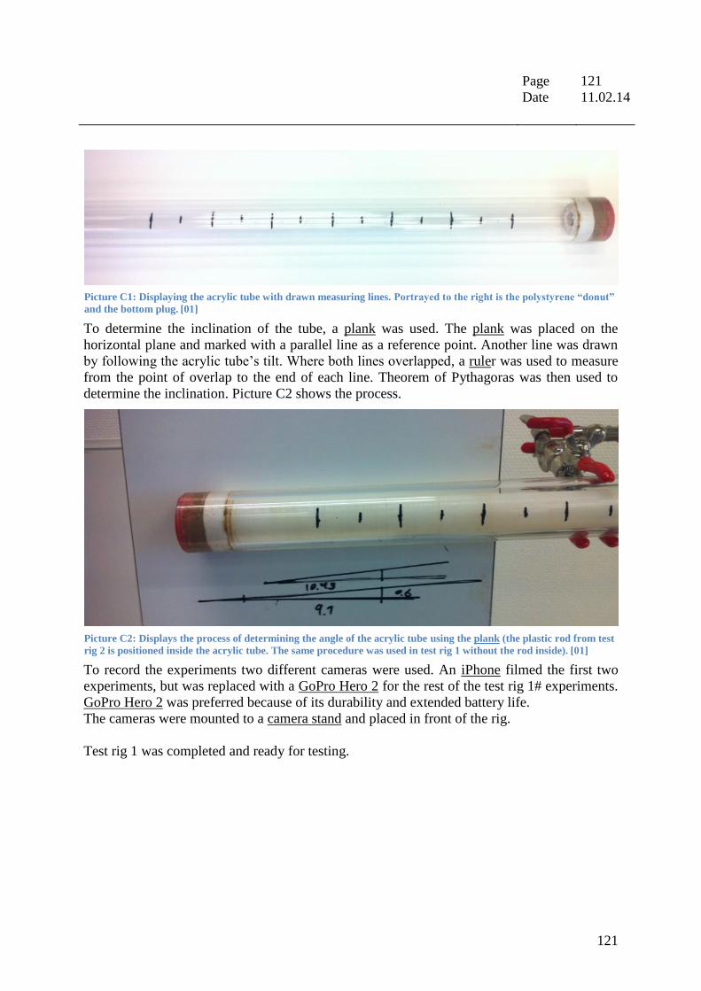
Page : 121

Date : 11.02.14

121

To determine the inclination of the tube, a plank was used. The plank was placed on the

horizontal plane and marked with a parallel line as a reference point. Another line was drawn

by following the acrylic tube’s tilt. Where both lines overlapped, a ruler was used to measure

from the point of overlap to the end of each line. Theorem of Pythagoras was then used to

determine the inclination. Picture C2 shows the process.

To record the experiments two different cameras were used. An iPhone filmed the first two

experiments, but was replaced with a GoPro Hero 2 for the rest of the test rig 1# experiments.

GoPro Hero 2 was preferred because of its durability and extended battery life.

The cameras were mounted to a camera stand and placed in front of the rig.

Test rig 1 was completed and ready for testing.

Picture C1: Displaying the acrylic tube with drawn measuring lines. Portrayed to the right is the polystyrene “donut”

and the bottom plug. [01]

Picture C2: Displays the process of determining the angle of the acrylic tube using the plank (the plastic rod from test

rig 2 is positioned inside the acrylic tube. The same procedure was used in test rig 1 without the rod inside). [01]

Page : 122

Date : 11.02.14

122

General specifications

Experiments conducted with test rig 1 contain diversities in regard to used equipment,

execution etc. but have some constant factors. In the subsections below these constant factors

and parameters for experiments performed with test rig 1 are listed.

Used equipment test rig 1


Equipment and tools utilized when performing experiments with test rig 1:

Beaker glass

Disposable syringe

Drill (1st)

Duct tape

Food dye

iPhone 4

Grease/lubricator

GoPro Hero 2

Laboratory stand

Plank

Small plastic pipe

Utility knife

Safety equipment

Safety glasses

Laboratory coat

Picture C3: Shows a sponge plug after it has been cut in to shape by the utility knife to the right. [01]

Page : 123

Date : 11.02.14

123

Experimental procedure

[All experiments conducted with test rig 1 followed the same procedure and execution]

1. The Acrylic tube was first filled with … (see experiment specification) using a beaker

glass.

2. A disposable syringe filled with ... (see experiment specification) dyed water topped

off the acrylic tube.

3. To seal off the tube, the sponge plugs pierced hole was lubricated and mounted with

the wood drill bit. The drill bit and sponge was then squeezed onto the top of the

acrylic tube with the help of a small plastic pipe, which drained the redundant air out

of the test system.

4. The filled and sealed acrylic was then positioned into a stand, which then was adjusted

to desired inclination (see experiment specification) using the plank (see picture 6).

5. The drill was then attached to a stand, and connected onto the drill bit.

6. A camera was positioned onto the camera stand and in front of the test rig to record

the experiment.

7. The experiment could now commence.

8. To start the experiment, a piece of duct tape was wrapped around the drills trigger.

9. Rotation began.

10. During the experiment, the extension of the mixing zone was recorded by following

the measurement lines on the acrylic tube. The time it took to reach the different lines

were documented at a later point using Adobe Premiere Pro C6.

11. After 20 min. of rotation, the experiment was ended by the duct tape being cut over

with a utility knife.

12. Rotation stopped.

13. The rig was dismantled and washed to make ready for the next experiment.

Page : 124

Date : 11.02.14

124

General uncertainties test rig 1

All experiments conducted with test rig 1 are exposed to certain general uncertainties. Listed

uncertainties apply for all tests performed with rig 1:

The interpretation of the spread of the

mixing zone done in Adobe Premiere Pro C6

is exposed to the human factor, and may

contain inaccuracies.

Stopping the experiment by cutting the duct

tape may cause the experiment to run longer

or shorter than intended. Estimated

uncertainty is ± 10 sec.

The inclination determined by the plank may

not be correct because of the uncertainties

this crude method is subjected to.

The stand that holds the acrylic tube is

exposed to unplanned disturbances, which

may disrupt the held inclination.

When sealing the acrylic tube with a sponge

plug, air may leak into the system. This can

affect the mixing of the fluids.

Because of the surface tension of the heavy

and light liquids the volume level read when

filling the acrylic tube may be inaccurate.

This can disrupt the planned ratio heavy light

liquid ratio.

Because of the limitations of the first drill an important factor as RPM couldn't be

varied in a constant and accurate rate. RPM for the experiments done with the first test

rig was therefore set as the maximum rotation rate of the drill (could vary depending

on the battery level of the drill). Using a GoPro Hero 2 and the video editing program

Adobe Premier Pro (see Appendix D) the speed of rotation was observed to be over

1000 RPM.

Picture C4: Displays the process of draining the acrylic

tube of excess air before execution of a experiment. [01]

Page : 125

Date : 11.02.14

125

Test rig 2



To construct test rig 2, following equipment and tools were used:

Industrial saw

Lathe

Sandpaper

Utility knife

Vernier Caliper

Water resistant marker pen

The second test rig was featured with the same components as the first, but had an additional

trait that made the system more similar to an actual drilling situation. Instead of having a

wood bit to simulate the wellhead, a plastic rod served as a replacement for the drill string.

This would expose the entire tube to the rotation, and not only a small percentage of the pipe.

The acrylic pipe would act as the wellbore while the plastic rod would represent the pipe. As

previously mentioned the ID of the acrylic pipe used in test rig 1# was 29,5 mm. With these 3

measurements it was possible to calculate the diameter of the plastic rod (see Appendix A for

equations):

With the correct diameter calculated, the fabrication of the plastic rod could begin.

A long plastic rod was cut to a length of 560 mm and lathed down from a diameter of 25,5

mm to the calculated 25,43 mm. As shown in the pictures C5 and C6 both ends were lathed

down to a diameter of 10 mm. The tip were the drill would be attached was lathed to a length

of 90 mm. These tips were also sanded down to minimize friction when rotating the rod. The

end caps would ensure stability and reduce vibrations in the system. When rotated this rod

would create a more realistic representation of Reelwells heavy over light method.

Picture C5: Showing the small tip being lathed and

sanded down to correct size. [01] Picture C6: The rod positioned into the lathe after

completing lathing the long tip. [01]

Page : 126

Date : 11.02.14

126

To stabilize and center the rod, a "donut" of polystyrene was positioned on top of the bottom

plug. The "donut" was designed to match the small tip of plastic rod and to prevent it from

creating uncontrolled disturbances.

Picture C7: The finished plastic rod. [01]

Page : 127

Date : 11.02.14

127

Test rig 2 general specifications

Experiments conducted with test rig 2 contains diversities in regard to used equipment,

execution etc. but has some constant factors. In the subsections below these constant factors

and parameters for experiments performed with test rig 2 are listed.



Equipment and tools used when performing experiments with test rig 2

Beaker glass

Disposable syringe

Drill (1st)

Duct tape

Food dye

Grease/lubricator

GoPro Hero 2

Plank

Small plastic pipe

Utility knife

Safety equipment

Safety glasses

Laboratory coat

Page : 128

Date : 11.02.14

128



1. The plastic rod was first placed into the acrylic tube, and centred by the polystyrene

"donut".

2. The acrylic tube was then filled with ... (see experiment specification) using a beaker

glass.

3. A disposable syringe filled with ... (see experiment specification) dyed water topped

off the acrylic tube.

4. To seal off the tube, the sponge plugs pierced hole was lubricated and mounted on the

long tip of the plastic rod. The sponge was then squeezed down the tip and onto the

top of the acrylic tube with the help of a small plastic pipe. The pipe drained the

redundant air out of the test system.


to desired inclination (see experiment specification) using the plank.


7. A camera was positioned onto the camera stand and in front of the test rig to record

the experiment.


9. To start the experiment, a piece of duct tape was wrapped around the drills trigger.

10. Rotation began.




12. After 20 min. of rotation, the experiment was ended by the duct tape being cut over

with a utility knife.



Page : 129

Date : 11.02.14

129


All experiments conducted with test rig 2 are exposed to certain general uncertainties. Listed

uncertainties apply for all tests performed with rig 1:

The sponge plug used in test rig 1 and 2 had an off-center hole which in experiments

conducted with rig 2 caused uneven rotation (effect assumed negligible on test rig 1).

This may have accelerated the development of the mixing zone. On the other hand this

mishap caused the test system to behave more realistically.

As for test rig 1, the cutting of the duct tape may cause the experiment to run longer or

shorter than intended. Estimated uncertainty is ± 10 sec.

As for test rig 1, the inclination determined by the plank may not be correct because of

the uncertainties this crude method are subjected to. An inaccurate inclination may

accelerate or reduce the expansion of the mixing zone.

The plastic rod has cyclical grooves after the lathing process (see picture 12). This can

affect the mixing zones propagation through the acrylic tube. The mixing impact of

these grooves will be investigated in experiments 14 and 15.

Picture C8: Close-up of the plastic rod, showing the lathe induced grooves. [01]

Page : 130

Date : 11.02.14

130

Test rig 3



During the construction of test rig 3 following equipment and tools were used:

Belt sander

Carpenter rule

Industrial saw

Lathe

Oxyacetylene torch

Sand paper

Silicon sealant

Soft hammer

Vernier caliper

Water resistant marker

White spray paint

The third and last test rig abandoned the main components from the two previous rigs. The

small tube was replaced with a 2000 mm long acrylic pipe with an OD of 38 mm and an ID of

32,0 mm. The pipe would make it possible to observe mixing distribution for a significantly

increased time and distance.

As in the construction of test rig 1, two plugs were made to contain the systems parameter:

Top plug: A foam based, conical plug made with the same material and

design as used for the sponge plug in test rig 1 and 2.

Bottom plug: A plastic, hat shaped plug lathed from a solid cylinder of hard

plastic. As shown in picture C9 it has two different sized ODs.

The smaller OD is designed to fit inside the acrylic tube, and

seal it of using seal rings. The larger diameter was cut to simplify

the fitting and the dismantling of the plug. A hole was also

drilled into the thinner part.

Picture C9: Displaying the plastic bottom plug; freshly fabricated to the right, and used to the left.

[01]

Page : 131

Date : 11.02.14

131

To create disturbances in the system, two different sized aluminum pipes were used. The

pipes were scaled after pipe and wellbore size data from Reelwell.

The pipe sizes 20 mm and 25 mm were used.

The aluminum pipes would be rotated inside the acrylic tube simulating a drill pipe inside a

wellbore (same principle as used in test rig 2).

To adapt the pipes to the system, they were cut down to 1900 mm using a carpenter rule and

an industrial saw. The edges were sanded down using a belt sander to remove excess metal

after the cut.

To prevent fluid from leaking into the aluminum pipes during experiments they were sealed

using 4 metal plugs (two for each pipe) which were lathed into shape. As shown in the picture

C10 there were two types of plugs; one long, which was placed on the top of the pipe and one

short for the lower end of the pipe. The two plugs were designed after the tips of the plastic

rod in the second test rig. The long tip would connect the pipe to the drill while the short

would be placed into the hole in the bottom plug and help stabilize the pipes rotation.

To connect the plugs to the aluminum pipes, a oxyacetylene torch heated the pipe ends and a

soft hammer hammered the metal plugs in. The four plugs were designed to be oversized to

ensure a tight fit. The belt sander and sandpaper were then used to sand down the

deformations of the pipes.

To secure that no fluid could enter the aluminum rods, silicon sealant was smeared into the

crack between the plug and the pipe.

To simplify the observation of the mixing zone the aluminum pipes were then painted white.

The pipes could now be mounted into the acrylic tube.

Picture C10: Showing the 4 metal plugs. [01]

Page : 132

Date : 11.02.14

132

As for test rig 1 and 2 measurement lines were drawn on the acrylic tube. A red, removable

marker was used to draw a uniform line along the pipe. A paper stencil was then positioned

along the line and a water resistant marker marked the measurement lines through it (see

picture C11). The measurement lines configuration was 20 mm between the short lines and

100 mm between the long lines.

After the lines had dried, the removable marker was washed away and the acrylic tube was

finished.

The main components of the third test rig were now complete and ready for assembly.

To run test rig 3 a new drill and trigger restraining method was needed. The new drill had

prolonged battery life and more power, which would contribute to the rigs stability and

reliability. To restrain the trigger two pre-tightened plastic strips were used (see picture …).

They were marked with red lines to differ them: 1 line = 150 RPM, 2 lines = 60 RPM.

All components of the rig were now ready.

The third test rig was now finished and experiment operative.

Picture C11: Displaying the paper stencil positioned on the acrylic tube. [01]

Picture C12: Showing the plastic strips around the drills handle. [01]

Page : 133

Date : 11.02.14

133

Test rig 3 general specifications

Experiments conducted with test rig 3 contained diversities in regard to equipment used,

execution etc. however some factors are kept constant throughout the tests. In the subsections

below these constant factors and parameters for experiments performed with test rig 3 are

listed.



Equipment and tools used when performing experiments with test rig 3

Beaker glass

Digital protractor

Disposable syringe

Drill (2nd

)

Grease/lubricator

GoPro Hero 2 and 3

Plastic strips (60 and 150 RPM)

Small plastic pipe

Workshop stand

Safety equipment

Safety glasses

Laboratory coat

Technical drawing 1: The technical drawing of the bottom plug. [04]

Page : 134

Date : 01.05.14

134



1. The plastic plug was first placed onto the lower part of the acrylic tube and sealed off.

2. Then a plastic hose was stuffed down the tube and the test rig was positioned vertical

onto a wall.

3. A beaker glass containing … (see experimental procedure) poured a previously

calculated volume through the hose and into the tube. The test rig was left standing for

5 minutes to drain the remaining fluid from the hose.

4. The plastic hose was then removed and the … (see experiment specification)

aluminum pipe was positioned into the acrylic tube. The test rig was then replaced

vertically onto a wall.

5. The remaining volume of the acrylic tube was then filled with ... (see experiment

specification) using a beaker glass.

6. To seal off the tube, the sponge plugs pierced hole was lubricated and mounted on the

long tip of the aluminum pipe. The sponge was then squeezed down the tip and onto

the top of the acrylic tube with the help of a small plastic pipe. The pipe drained the

redundant air out of the test system.


to desired inclination (see experiment specification) using a digital protractor.


9. A camera (GoPro 2 and 3) was positioned onto the camera stand and in front of the

test rig to record the experiment.


11. To start the experiment, one of two pre tightened plastic strips were placed around the

drills trigger.

12. Rotation began.




14. After 60 min. of rotation, the experiment was ended by removing the plastic strip from

the drills trigger.



Page : 135

Date : 01.05.14

135


All experiments conducted with test rig 3 were exposed to certain general uncertainties.

Listed uncertainties apply for all tests performed with rig 1:

Both aluminum pipes have slightly off-center long tips, which caused unplanned

movement of the pipes when they were exposed to rotation. This may have accelerated

the propagation of the mixing zone. On the other hand, this design flaw caused the

pipe to move more realistically around in the acrylic tube rather than an unlikely

centered rotation.

The plastic strips used to hold the drills trigger in place were subjected to uncertainties

which may have caused higher or lower rotational speeds in certain experiments. The

increase or decrease in pipe RPM may have caused an accelerated or decelerated

movement of the mixing zone.

Picture C13: Displays the process of cleaning the long acrylic tube using paper towels as an improvised “Pig”. [01]

Page : 136

Date : 01.05.14

136

Viscometer test rig Test rig construction and setup


To construct viscometer test rig, the following equipment and tools were used:

Ruler

Utility knife

Vernier Caliper

The viscometer test rig was comprised of two components: A viscometer and a plastic cup.

The viscometer was kept in original shape as described in Appendix D. The plastic cup was

made out of a water bottle. The bottle was measured using a ruler to the desired height and cut

in two using an utility knife. Depth and diameter was later measured (using a Vernier caliper)

to 150 mm and 56,3 mm. A scale was then positioned on the side of the cup, and the test rig

was complete

Viscometer test rig general specifications

Experiments conducted with viscometer test rig contained diversities in regard to equipment

used, execution etc. however some factors are kept constant throughout the tests. In the

subsections below these constant factors and parameters for experiments performed with

viscometer test rig are listed.

Used equipment viscometer test rig


Equipment and tools used when performing experiments with viscometer test rig

Beaker glass

Disposable syringe

GoPro Hero 2

Viscometer

Safety equipment

Safety glasses

Laboratory coat

Page : 137

Date : 01.05.14

137


[The two experiments conducted with Viscometer test rig followed the same procedure and execution]

1. The plastic cup was first filled 2/3 of the total fluid volume with ... (see experiment

specification) using a beaker glass.

2. A disposable syringe filled 1/3 of the total fluid volume with … (see experiment

specification) into the plastic cup.

3. The cup was then positioned onto the Viscometer.

4. The experiment could begin.

5. RPM was gradually increased in the viscometers RPM intervals (3, 6, 100, 200) until

heavy light mixing was complete.


General uncertainties viscometer test rig

The two experiments conducted with Viscometer test rig were exposed to certain general

uncertainties. Listed uncertainties apply for the two tests performed with the viscometer test

rig:

The general uncertainty of the Viscometer in question applies for the two experiments.

The RPM settings may be inaccurate, which would affect the perceived mixing at the

specific RPM.

The plastic cup may not have been positioned in the middle of the Viscometer. This

may have affected the mixing effect.

Page : 138

Date : 01.05.14

138

Appendix D – Equipment/tools

Measuring equipment

Nr Name Description Picture [01]

M1 Adobe

Premier Pro

C6

A high grade editing

program used to

shape and alter any

type of video. Used

as a measurement

equipment together

with GoPro Hero2

when determining

RPM.

M2 Digital

protractor

Digital tool used to

measure the angle of

flat surfaces and

other tilted objects. It

is fitted with a

tubular spirit level

that ensures that the

measurement is

taken with a

perfectly horizontal

plane as a reference

point. Has a angular

resolution of 0,1o and

a measurement

accuracy of ±0,5o.

M3 Disposable

syringe

A device used to

precisely measure a

small quantity of

liquid. Has a max

capacity of 60 ml.

Page : 139

Date : 01.05.14

139


M4 Laboratory scale An accurate measuring

tool used to precisely

weigh small quantities of

different experimental

components or

ingredients.

The scale is able to

measure down to 1/10 of

a gram.

M5 Mud

balance/scale

A device used to measure

the density of any type of

liquid such as drilling

fluids and other viscous

liquids.

M6 Plank A tool used together with

a marker pen to determine

angles.

Page : 140

Date : 01.05.14

140


M7 Ruler/carpenters

rule

Measuring device used to

measure small distances.

M8 Vernier Caliper Measuring tool

specialized for measuring

OD, ID and depth of tubes

and pipes. The Vernier

Calipers provide a

precision to 0.01 mm or a

1/1000 of an inch. Can

measure accurately up to

182,9 mm or 7,2 inch.

M9 Viscometer An instrument used to

measure the viscosity of a

fluid. It rotates a tube at

different RPM's that is

dipped into the tested

fluid. Inside the tube there

is a spring mounted

cylinder which reacts to

the different rotation

speeds and the viscosity

of the fluid. The

movement of this cylinder

is displayed on a scale on

the top of the device.

Page : 141

Date : 01.05.14

141

Experiment tools


E1 Beaker glass A container of glass

which purpose is to retain

a measured amount of

liquid and be able to pour

this liquid in a controlled

manner.

E2 Camera stand A stand used to support

the cameras, and position

them in the right place

and height.

Page : 142

Date : 01.05.14

142


E3 Drill [Pictures on the right from the

top;

Drill nr. 1 and nr. 2]

A tool designed to rotate

devices/objects at

different speeds and

torque.

E4 Duct tape A strong tape used to

restrain and secure objects

for a period of time.

Page : 143

Date : 01.05.14

143


E5 Food dye [The picture shows only one of

many food dyes used]

An additive used to color

fluid and liquids. This

helps with distinguishing

them from each other.

E6 GoPro Hero

(2/3)

A action camera used to

film high quality footage.

The camera is able to film

with high frame rates

(FPS), allowing for slow

motion. Combined with

the editing program

Adobe Premier Pro C6

and the marker tape, the

GoPro is used to

determine RPM.

E7 Grease/lubricator A lubricating element

used to decrease friction

and heat generation in the

interface between a

stagnant and a moving

object.

Page : 144

Date : 01.05.14

144


E8 iPhone 4 [Picture taken with another

iPhone 4]

A smart mobile telephone

fitted with among other

things, video recording

capabilities. Used to

document experiments

before the GoPro Hero2

was put to use.

E9 Laboratory stand A stand is designed to

place and secure

laboratory equipment in

desired positions.

E10 Marker tape

[Pictures on the right from the

top;

Marker tape nr. 1 and nr. 2]

A piece of tape placed on

a rotating object to be

able to determining its

RPM. This is done

together with Adobe

Premiere Pro C6 and

GoPro Hero 2 and 3.

E11 Paper stencil A tool used to produce

constant shapes on an

underlying surface by

applying pigment.

Page : 145

Date : 01.05.14

145


E12 Plastic hose An elastic plastic tube

used to transport liquid

from one point to another

in a clean manner.

E13 Plastic strips A tool designed to

restrain small objects

E14 Small plastic

pipe

A device used to remove

excess air.

E15 Thread seal tape A low friction tape which

molds itself when put

under pressure. Is most

commonly used to seal

threads and other tight

fits.

E16 Utility knife

A tool used to cut and

shape soft objects.

E17 Workshop stand Stand used to stabilize

cylindrical objects.

Page : 146

Date : 01.05.14

146

Fabrication Equipment


F1 Belt sander

A grinding tool fitted

with a seamless loop

of abrasive sandpaper

which is rotated at

high speed. The belt

sander is mainly used

to grind down metal

parts into a desired

shape.

F2 Industrial saw A heavy duty saw

designed to cut metal

and hard plastics in a

fast and safe manner.

The saw has a nozzle

which sprays coolant

on the saw blade to

ensure minimum heat

development in the

material.

F3 Lathe An equipment/tool

used to reduce the

diameter and size of

circular metal and

hard plastic objects.

It is fitted with

carbide cutting tools

which shave off

pieces of the rotated

material.

Page : 147

Date : 01.05.14

147


F4 Oxyacetylene

torch

An oxyacetylene powered

torch used to cut and heat

metal objects. The torch

can also be used for

soldering.

F5 Sand paper An abrasive paper

designed to file different

objects down to the

desired shape.

F6 Silicon sealant A tool used to seal gaps

and cracks from intruding

liquids.

F7 Soft hammer A hammer designed with

soft tips. This is done to

protect the object that is

being hammered from

unnecessary deformations

and damages.

F8 Water resistant

marker pen

Pen used to mark and

draw on objects that are

exposed to water and

other liquids.

F9 White spray

paint

Spray paint used to cover

various surfaces.

Page : 148

Date : 01.05.14

148

Safety equipment


S1 Gloves -

workshop and

welding

Gloves used to protect

the hands from warm and

sharp objects.

S2 Laboratory coat Protective gear used to

shield the body from

exposure to dangerous

elements, mainly liquids.

S3 Protective

glasses

Glasses built to withstand

small high-speed

projectiles and protect

the eyes from other

hazardous objects or

liquids.

Page : 149

Date : 01.05.14

149

Appendix E – List of charts Page

Chart 1: The flow pattern of test rig 2 experiments conducted with Syrup 2 and water. [02] 59

Chart 2: Shown the flow pattern of experiments conducted with OBM 1 and olive oil. [02] 67

Chart 3: The flow pattern for experiments conducted according to Matrix 1. [02] 80

Chart 4: Displays the flow pattern of experiment 25. [02] 82

Chart 5: The flow pattern of the experiments conducted in matrix 2. [02] 86

Chart 6: The flow pattern of experiments 30 and 31. [02] 90

Chart 7: Viscometer experiment 2s flow pattern. [02] 96

Chart 8: Displaying the flow pattern differences between two pipe sizes. [02] 102

Chart 9: Displaying the flow pattern differences between two pipe sizes. [02] 102

Chart 10: Displaying the flow pattern differences between two RPM. [02] 104

Chart 11: Displaying the flow pattern differences between three RPM for

Reelwell scenario 1. [02] 105

Chart 12: Displaying the flow pattern differences between three RPM for

Reelwell scenario 2. [02] 105

Page : 150

Date : 01.05.14

150

Appendix F – List of figures

Figures Page

Figure 1: Extended reach drilling envelope. [07] 6

Figure 2: Comparison of Conventional drainage area vs. Reelwell drainage area. [R02] 7

Figure 3: Displays Reelwells heavy over light concept. [R02] 7

Figure 4: Illustrates Reelwells heavy over light method. [R02] 8

Figure 5: Figures illustrating how inclination is perceived in the thesis. [04] 9

Figure 6: Displays the heavy light setup with all RDM components. [R03] 11

Figure 7: Bottom view of a rotation drill pipe in a wellbore. [04] 15

Figure 8: Helical flow of YPL fluid in concentric annulus. [T05] 20

Figure 9: Displays the three flow regimes. [T02] 23

Figure 10: The heavy light fluid scenario displayed with the applicable component names and

setup. [04] 24

Figure 11: Showing the assumed heavy light interface when only the force of gravity affects

the fluids. The dashed lines running throughout the figure represent the drill pipe. [04] 25

Figure 12: Showing the assumed heavy light interface when the forces of gravity and rotation

affect the fluids. The dashed lines running throughout the figure represent the drill pipe. [04]

25

Figure R1: Conventional vs. RDM technology [R02] 115

Figure R2: The opening sequence of Reelwells DFV. [R05] 118

Figure R3: The closing sequence of Reelwells DFV. [R05] 118

Figure R4: Reelwell hydraulic WOB. [R01] 119

Technical drawing 1: The technical drawing of the bottom plug. [04] 133

Pictures

Page Picture 1: Test rig 1 # layout with used equipment positioned for a test of feasibility

of future experiments. The acrylic pipe displayed has an inclination of 3,3o

relative to the horizontal plane. The wood bit is as showed mounded trough

the sponge plug into the drill. Weights are placed on both stands to ensure stability. [01] 33

Picture 2: Test rig 2 # setup with used equipment positioned for a test of feasibility

of future experiments. The acrylic pipe displayed has an inclination of 3,3o

relative to the horizontal plane. The plastic rod is mounded trough the sponge plug

into the drill. Weights are placed on both stands to ensure stability. [01] 48

Page : 151

Date : 01.05.14

151

Picture 3: Test rig 3 # setup with used equipment positioned for a test of feasibility of

future experiments. The acrylic pipe displayed has an inclination of 2,0o relative to the

horizontal plane. The 20 mm diameter aluminum pipe is mounded through

the sponge plug into the drill. The drill are fitted with different tensioned

plastic strips Weights are placed on both stands to ensure stability, while

the workshop stand holds the heavy end in angle. [01] 70

Picture 4: Viscometer test rig setup. The plastic cup is displayed positioned

onto the Viscometers steel cylinder, filled with fluids form the first experiment.

The scale to the left is placed to simplify the observation of

the mixing zone movement. [01] 92

Picture C1: Displaying the acrylic tube with drawn measuring lines. Portrayed to

the right is the polystyrene “donut” and the bottom plug. [01] 121

Picture C2: Displays the process of determining the angle of the acrylic tube using

the plank (the plastic rod from test rig 2 is positioned inside the acrylic tube.

The same procedure was used in test rig 1 without the rod inside). [01] 121

Picture C3: Shows a sponge plug after it has been cut in to shape by the utility

knife to the right. [01] 122

Picture C4: Displays the process of draining the acrylic tube of excess air before

execution of a experiment. [01] 124

Picture C5: Showing the small tip being lathed and sanded down to correct size. [01] 125

Picture C6: The rod positioned into the lathe after completing lathing the long tip. [01] 125

Picture C7: The finished plastic rod. [01] 126

Picture C8: Close-up of the plastic rod, showing the lathe induced grooves. [01] 129

Picture C9: Displaying the plastic bottom plug; freshly fabricated to the right, and

used to the left. [01] 130

Picture C10: Showing the 4 metal plugs. [01] 131

Picture C11: Displaying the paper stencil positioned on the acrylic tube. [01] 132

Picture C12: Showing the plastic strips around the drills handle. [01] 132

Picture C13: Displays the process of cleaning the long acrylic tube using paper

towels as an improvised “Pig”. [01] 135

Page : 152

Date : 01.05.14

152

Appendix G – List of graphs Page

Graph 1: Displays buoyancy effects on drag in a RDM drilling scenario. [R03] 13

Graph 2: Shows the effect of buoyancy and drill pipe material has on torque. [R03] 15

Graph 3: Displays the models shear stress-shear rate behavior. [T03] 17

Graph 4: Displaying the distribution of density in the mixing zone. [02] 26

Graph 5: Displays the fluid rheology to the liquids used in test rig 1#. [02] 40

Graph 6: Illustrates the propagation of the mixing interface for all applicable

experiments conducted with test rig 1#. [02] 41

Graph 7: Displays the effect of inclination gained from experiment 1, 2 and 3. [02] 42

Graph 8: Trend lines of the curves displayed in graph 6. [02] 43

Graph 9: Visual presentation of inclinations effect on mixing distance and

mixing rate. [02] 43

Graph 10: Displays the data gained from experiment 4. [02] 44

Graph 11: Displays the data gained from experiment 7. [02] 45


Graph 13: Illustrates the propagation of the mixing interface for all applicable

experiments conducted with test rig 2#. [02] 59

Graph 14: Displays the effect of CW and ACW gained from experiment 14 and 15. [02] 63


Graph 16: Displays the mixing effect of heavy OBM and negative inclination

gained from experiments 17, 19 and 20. [02] 66



Graph 19: Displays the fluid rheology to OBM 1, 2 and 3. [02] 77


Graph 21: Displays the mixing effect of RPM and pipe size gained from

experiments 21, 22, 23 and 24. [02] 79



experiments 21, 22, 23 and 24. [02] 81


experiments 26, 27, 28 and 29. [02] 84


Page : 153

Date : 01.05.14

153

Graph 26: Displays the mixing effect of negative inclination gained from

experiments 30 and 31. [02] 88


Graph 28: Displays the areas of surge and reduced mixing in experiment 31. [02] 89


Graph 30: Displays the mixing slopes of experiments conducted with positive and

negative inclination. [02] 100

Graph 31: Displays the difference in heavy light interface movement between

two pipe sizes. [02] 101

Graph 32: Displays the mixing effect of two different RPM. All other parameters

than the RPM of the pipes is held constant. [02] 104

Graph 33: Displays the effect of low viscous light fluid have on mixing propagation

in test rig 3. [02] 106

Graph 34: Displays the effect of Yield point differences have on mixing propagation

in test rig 3. [02] 108

Page : 154

Date : 01.05.14

154

Appendix H – List of tables

Tables Page

Table 1: Effect of density difference on buoyancy. [R03, 02] 12

Table 2: Reelwell heavy light fluid properties. [R05] 28

Table 3: Mud formulation and ingredients. [05] 30

Table 4: Trial and error diesel rapeseed ratio. 31

Table 5: Test rig 1# setup specifics. 33

Table 6: Shows the technical data for experiments 1, 2 and 3. [02] 34

Table 7: Shows the technical data for ex. 4 and 6. [02] 36

Table 8: Displays the technical data for ex. 5 and 7. [02] 38

Table 9: Showing the fluid properties for the heavy liquids used in test rig 1#. [02] 40

Table 10: Displaying the numerical data for the three experiments. 43

Table 11: Summary of viable results from test rig 1#. 46

Table 12: Test rig 2# setup specifics. 48


Table 14: Displays the technical data for ex. 10, 11, 12 and 13. [02] 51



Table 17: Displays the technical data for ex. 17, 19 and 20. [02] 56


58


Table 20: Aluminum pipe OD calculation. [02] 69

Table 21: Test rig 3# specifics. 69


Table 23: Displays the technical data for ex. 25. [02] 73




76

Table 27: Displays matrix nr. 1. 79

Table 28: Displays the mixing zone movement results from ex. 21, 22, 23 and 24. [02] 80

Page : 155

Date : 01.05.14

155

Table 29: Displays the mixing zone movement result from ex. 25. [02] 82

Table 30: Displays matrix nr. 2. 84

Table 31: Displays the mixing zone movement results from ex. 26, 27, 28 and 29. [02] 85

Table 32: Displays the mixing zone movement results from ex. 30 and 31. [02] 89


Table 34: Viscometer test rig specifics. 92

Table 35: Displays the technical data for viscometer ex. 1 and 2. [02] 93


94

Table 37: Displays the two Reelwell scenarios wellbore and drill pipe diameter. [R05] 97

Table 38: Parameter information. [R05] 97

Table 39: Reelwell fluid configuration. [R05] 97

Table 40: Showing the calculation of scenario 1 and 2s mixing zone lengths. 98

Table 41: Showing the calculation of scenario 1 and 2s mixing zone length. 99

Table 42: Displaying various experiments 99

Table 43: Mixing distance and rate for PV 107

Table 44: Mixing distance and rate for PV 4, 20 and 65 scaled up to scenario 1 and 2. 107

Table 45: Displays the parameters effect on mixing zone movement. 109

Table 46: Abbreviation table. 111

Table 47: Table of equations. 114

Screenshot tables Page

Screenshot table 1: Screenshots from the experimental footage taken under the

execution of experiments 1, 2 and 3. [03] 42

Screenshot table 2: Screenshots of the experimental footage from the execution of


Screenshot table 3: Screenshots of the experimental footage from execution of


Screenshot tables 4: Screenshots from the experimental footage taken under the

execution of experiments 8 and 9. [03] 60

Screenshot tables 5: Screenshots from the footage taken under the execution of

experiments 10, 11, 12 and 13. [03] 61



Page : 156

Date : 01.05.14

156

Screenshot tables 7: Screenshots from experimental the footage taken under the



execution of experiments 17, 19 and 20. [03] 65

Screenshot tables 9: Screenshots from ex. footage taken under the execution of

experiments 21, 22, 23 and 24. The bended illustration of some of the experiments

is due to a fish eyed lens, not experiment setup. [03] 78


experiment 25. The bended illustration of some of the experiments screenshots

are due to a fish eyed lens, not experiment setup. [03] 81


experiments 26, 27, 28 and 29. The bended illustrations of some of the experiments

are due to a fish eyed lens, not experiment setup. [03] 83


experiments 30 and 31. Screenshots from experiment 31 is taken two different cameras.

The second camera took over when the mixing zone had moved passed the range

of the lens. As seen in the top of the third screenshot from the left, the mixing zone

is moving downwards. The bended illustration of some of the experiments

is due to a fish eyed lens, not experiment setup. [03] 87


viscometer experiments 1 and 2. [03] 95

Page : 157

Date : 01.05.14

157

Attachment – Experimental CD

Experimental data are available in the attached CD at the back cover of the thesis.

Documents

MASTER’S THESIS - Bibsys · MASTER’S THESIS Study program ... information for the overall heavy light setup design and the development of the operation ... What is the extent