Mat and Inventory

Presented By

Niaz Ahmed CSCM, MBA in MIS (DU), B.Sc in ME (MIST)

Material And Inventory Management

Welcome to Day Long Training on

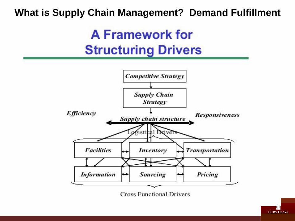
What is Supply Chain Management? Demand Fulfillment

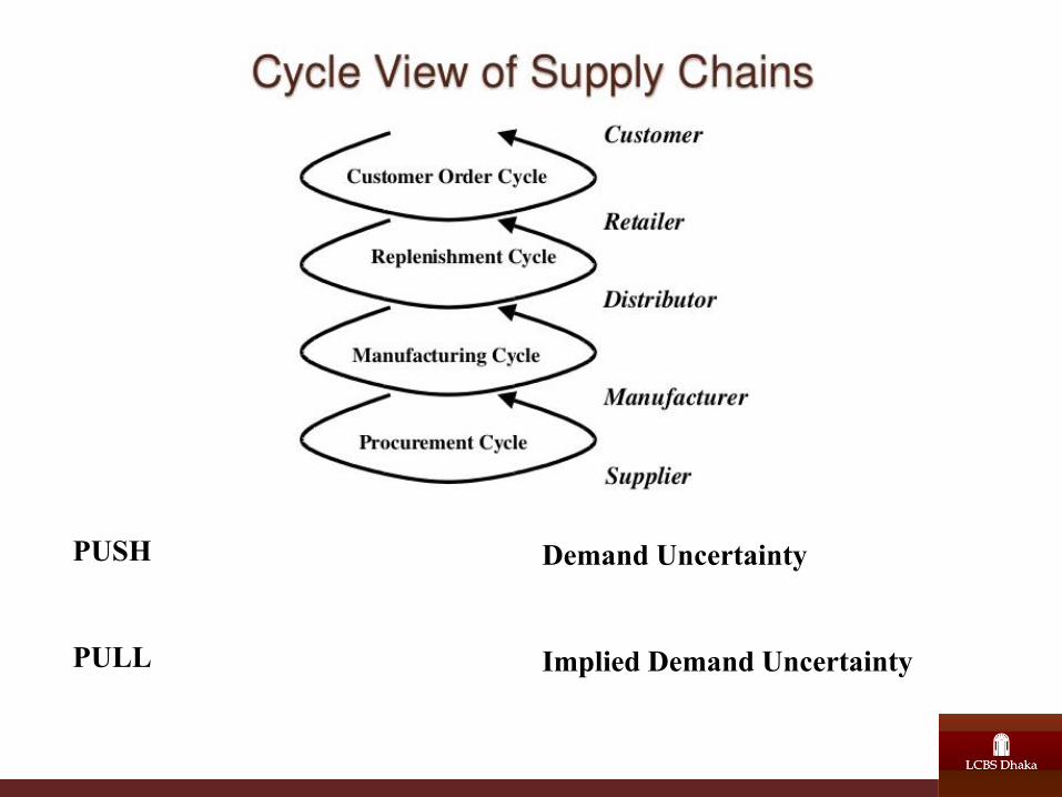
PUSH

PULL

Demand Uncertainty

Implied Demand Uncertainty

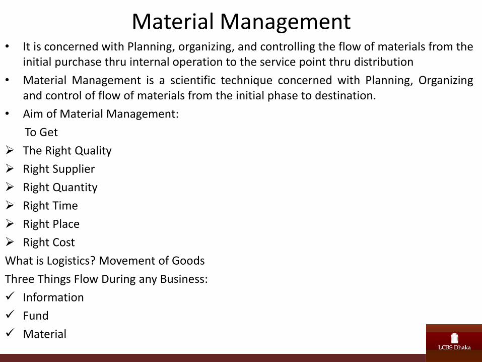
Material Management • It is concerned with Planning, organizing, and controlling the flow of materials from the

initial purchase thru internal operation to the service point thru distribution

• Material Management is a scientific technique concerned with Planning, Organizing and control of flow of materials from the initial phase to destination.

• Aim of Material Management:

To Get

The Right Quality

Right Supplier

Right Quantity

Right Time

Right Place

Right Cost

What is Logistics? Movement of Goods

Three Things Flow During any Business:

Information

Fund

Material

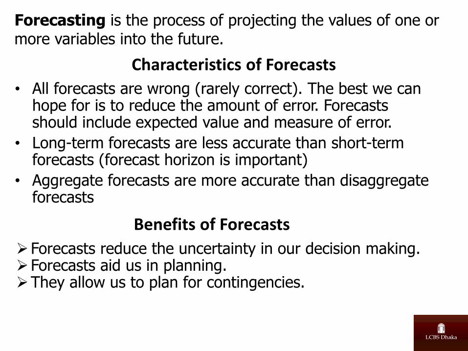
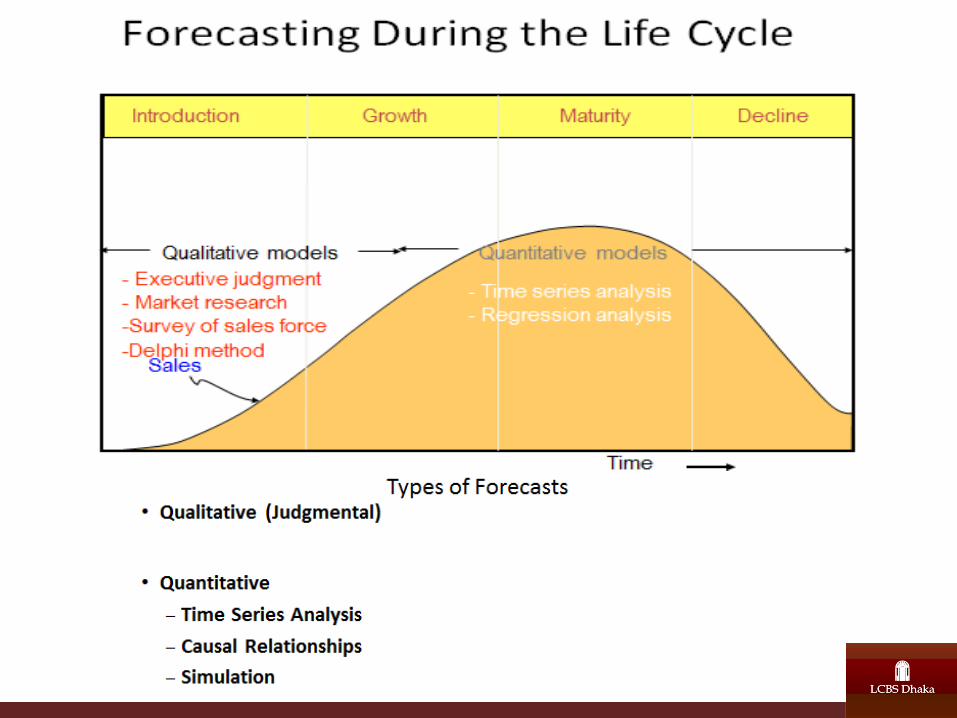
Characteristics of Forecasts

• All forecasts are wrong (rarely correct). The best we can hope for is to reduce the amount of error. Forecasts should include expected value and measure of error.

• Long-term forecasts are less accurate than short-term forecasts (forecast horizon is important)

• Aggregate forecasts are more accurate than disaggregate forecasts

Forecasting is the process of projecting the values of one or more variables into the future.

Forecasts reduce the uncertainty in our decision making. Forecasts aid us in planning. They allow us to plan for contingencies.

Benefits of Forecasts

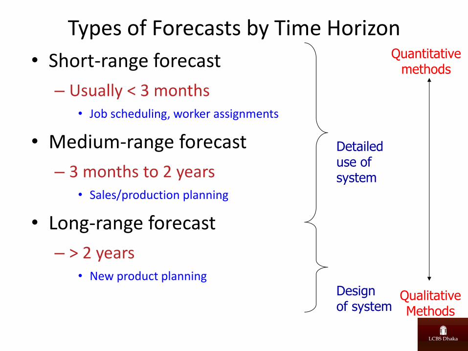
Types of Forecasts by Time Horizon

• Short-range forecast

– Usually < 3 months • Job scheduling, worker assignments

• Medium-range forecast

– 3 months to 2 years • Sales/production planning

• Long-range forecast

– > 2 years • New product planning

Design of system

Detailed use of system

Quantitative methods

Qualitative Methods

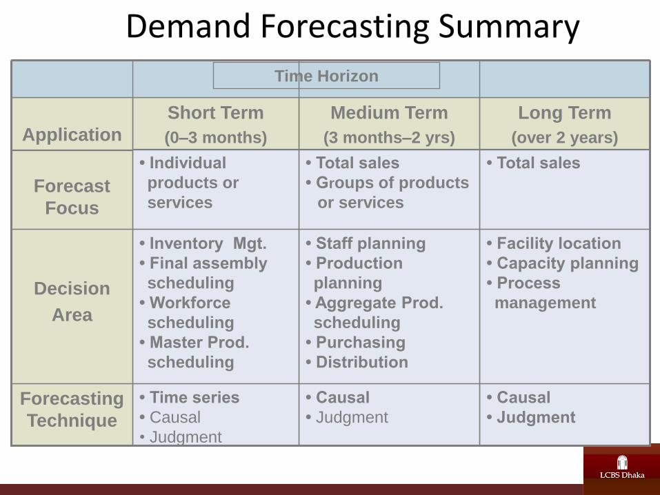
• Causal

• Judgment

• Causal

• Judgment

• Time series

• Causal

• Judgment

Forecasting

Technique

• Facility location

• Capacity planning

• Process

management

• Staff planning

• Production

planning

• Aggregate Prod.

scheduling

• Purchasing

• Distribution

• Inventory Mgt.

• Final assembly

scheduling

• Workforce

scheduling

• Master Prod.

scheduling

Decision

Area

• Total sales • Total sales

• Groups of products

or services

• Individual

products or

services

Forecast

Focus

Long Term

(over 2 years)

Medium Term

(3 months–2 yrs)

Short Term

(0–3 months)

Application

Time Horizon

Demand Forecasting Summary

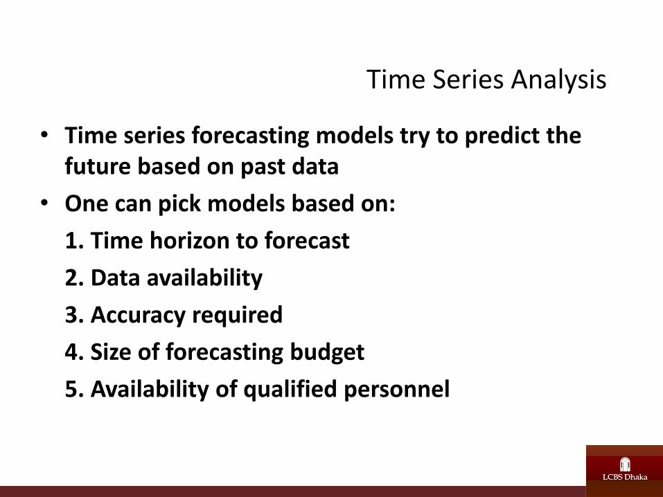
Time Series Analysis

• Time series forecasting models try to predict the future based on past data

• One can pick models based on:

1. Time horizon to forecast

2. Data availability

3. Accuracy required

4. Size of forecasting budget

5. Availability of qualified personnel

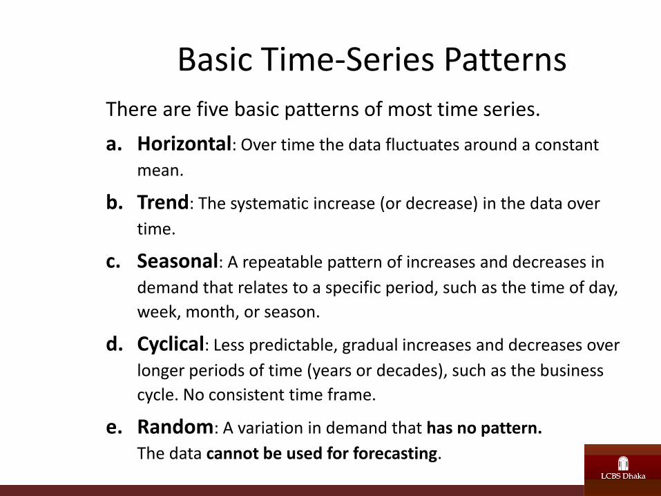
Basic Time-Series Patterns There are five basic patterns of most time series.

a. Horizontal: Over time the data fluctuates around a constant

mean.

b. Trend: The systematic increase (or decrease) in the data over

time.

c. Seasonal: A repeatable pattern of increases and decreases in

demand that relates to a specific period, such as the time of day,

week, month, or season.

d. Cyclical: Less predictable, gradual increases and decreases over

longer periods of time (years or decades), such as the business

cycle. No consistent time frame.

e. Random: A variation in demand that has no pattern.

The data cannot be used for forecasting.

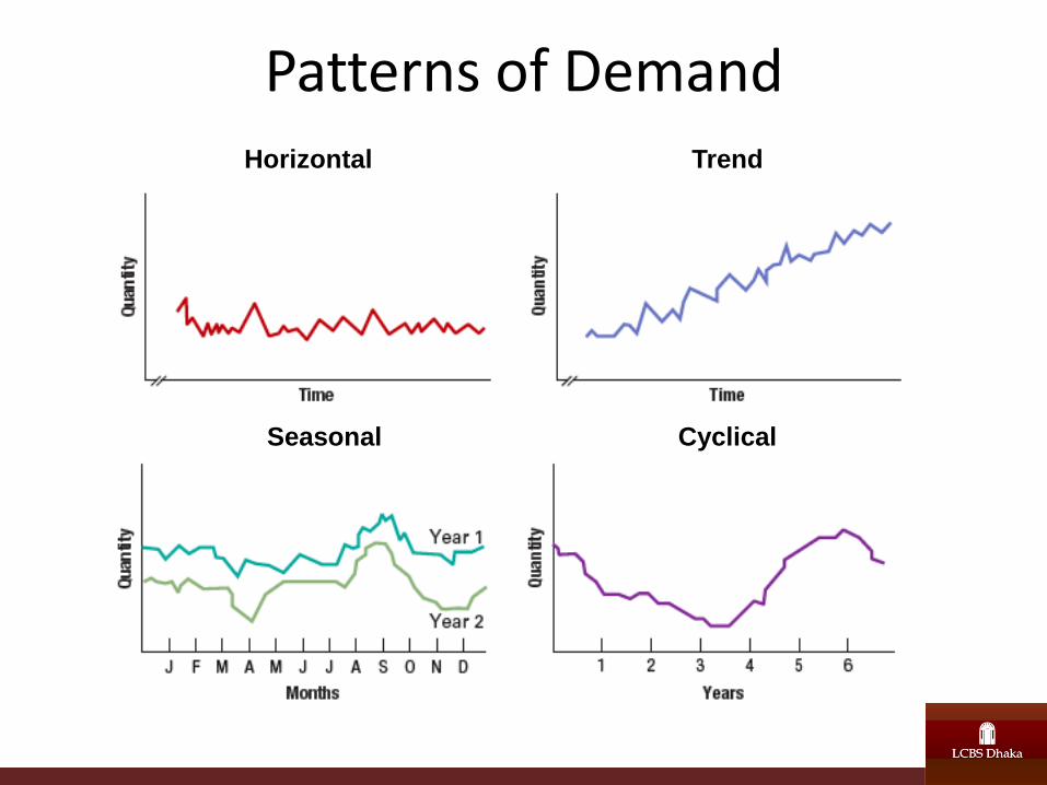
Patterns of Demand Horizontal Trend

Seasonal Cyclical

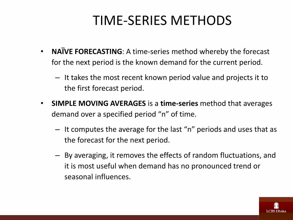
TIME-SERIES METHODS

• NAÏVE FORECASTING: A time-series method whereby the forecast

for the next period is the known demand for the current period.

– It takes the most recent known period value and projects it to

the first forecast period.

• SIMPLE MOVING AVERAGES is a time-series method that averages

demand over a specified period “n” of time.

– It computes the average for the last “n” periods and uses that as

the forecast for the next period.

– By averaging, it removes the effects of random fluctuations, and

it is most useful when demand has no pronounced trend or

seasonal influences.

Simple Moving Averages

22 becomes the forecast for week #5 23.25 becomes the

forecast for week #6.

This is a 4-period moving average.

The moving average method involves the use of as many periods

of past demand as desired or deemed appropriate. The stability of

the demand series generally determines how many periods.

WEEK DEMAND AVERAGE

1 20

2 23

3 21

4 24 22

5 25 23.25

6 ?

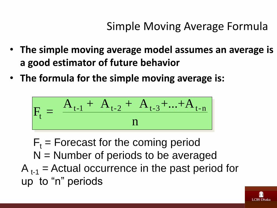
Simple Moving Average Formula

• The simple moving average model assumes an average is a good estimator of future behavior

• The formula for the simple moving average is:

F = A + A + A +...+A

nt

t-1 t-2 t-3 t-n

Ft = Forecast for the coming period

N = Number of periods to be averaged

A t-1 = Actual occurrence in the past period for

up to “n” periods

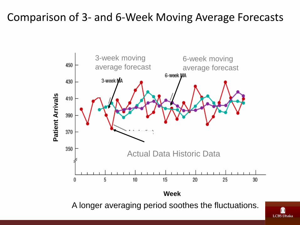
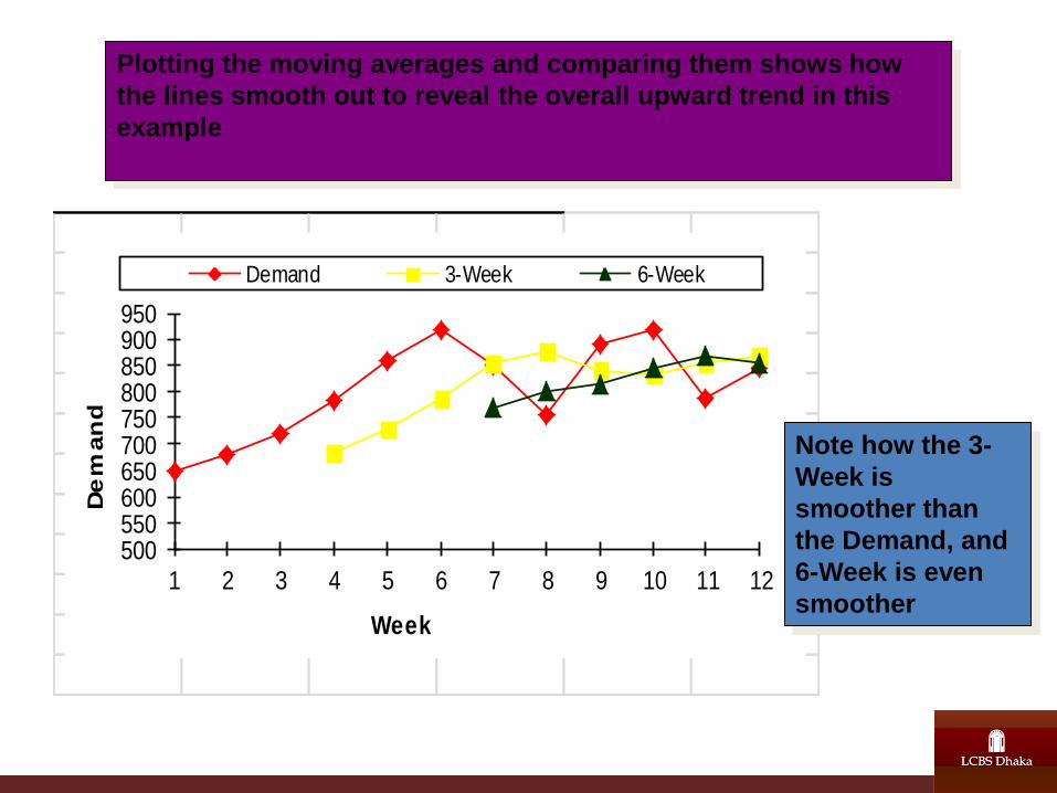
Comparison of 3- and 6-Week Moving Average Forecasts

Week

Pati

en

t A

rriv

als

Actual Data Historic Data

3-week moving

average forecast 6-week moving

average forecast

A longer averaging period soothes the fluctuations.

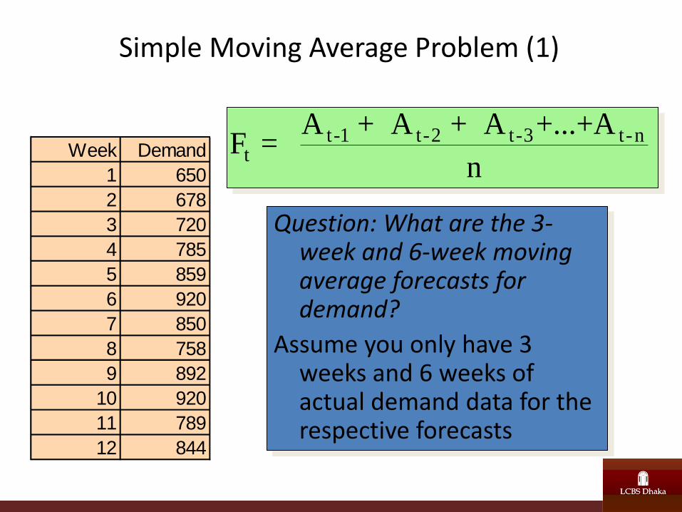
Simple Moving Average Problem (1)

Question: What are the 3-week and 6-week moving average forecasts for demand?

Assume you only have 3 weeks and 6 weeks of actual demand data for the respective forecasts

Week Demand

1 650

2 678

3 720

4 785

5 859

6 920

7 850

8 758

9 892

10 920

11 789

12 844

F = A + A + A +...+A

nt

t-1 t-2 t-3 t-n

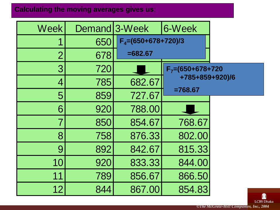
Week Demand 3-Week 6-Week

1 650

2 678

3 720

4 785 682.67

5 859 727.67

6 920 788.00

7 850 854.67 768.67

8 758 876.33 802.00

9 892 842.67 815.33

10 920 833.33 844.00

11 789 856.67 866.50

12 844 867.00 854.83

F4=(650+678+720)/3

=682.67

F7=(650+678+720

+785+859+920)/6

=768.67

Calculating the moving averages gives us:

©The McGraw-Hill Companies, Inc., 2004

500550600650700750800850900950

1 2 3 4 5 6 7 8 9 10 11 12

De

man

d

Week

Demand 3-Week 6-Week

Plotting the moving averages and comparing them shows how

the lines smooth out to reveal the overall upward trend in this

example

Note how the 3-

Week is

smoother than

the Demand, and

6-Week is even

smoother

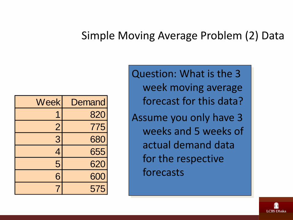
Simple Moving Average Problem (2) Data

Question: What is the 3 week moving average forecast for this data?

Assume you only have 3 weeks and 5 weeks of actual demand data for the respective forecasts

Week Demand

1 820

2 775

3 680

4 655

5 620

6 600

7 575

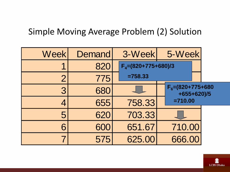
Simple Moving Average Problem (2) Solution

Week Demand 3-Week 5-Week

1 820

2 775

3 680

4 655 758.33

5 620 703.33

6 600 651.67 710.00

7 575 625.00 666.00

F4=(820+775+680)/3

=758.33

F6=(820+775+680

+655+620)/5

=710.00

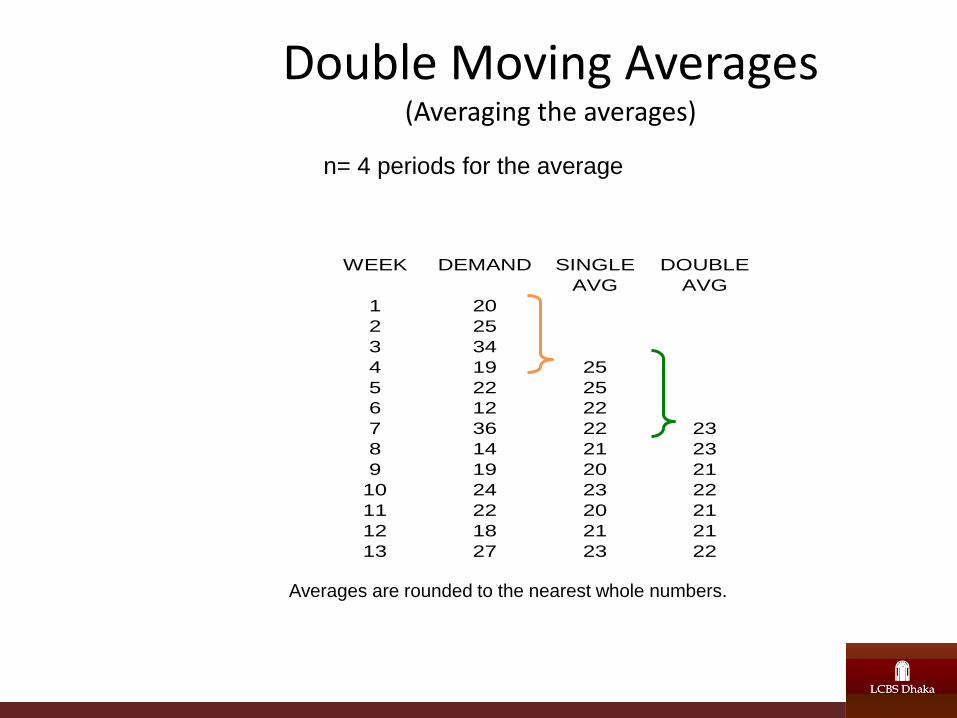
WEEK DEMAND SINGLE DOUBLE

AVG AVG

1 20

2 25

3 34

4 19 25

5 22 25

6 12 22

7 36 22 23

8 14 21 23

9 19 20 21

10 24 23 22

11 22 20 21

12 18 21 21

13 27 23 22

Double Moving Averages (Averaging the averages)

n= 4 periods for the average

Averages are rounded to the nearest whole numbers.

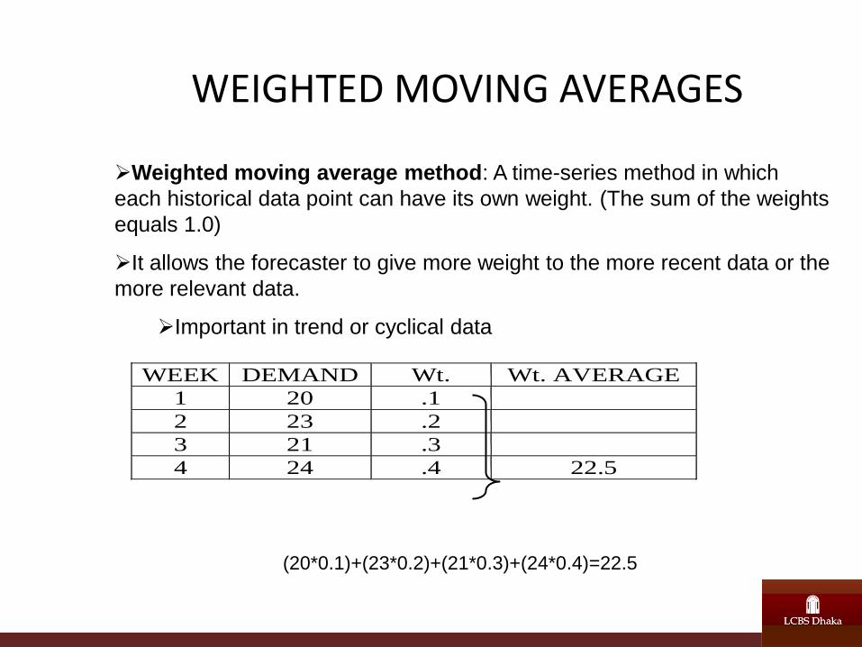
WEEK DEMAND Wt. Wt. AVERAGE

1 20 .1

2 23 .2

3 21 .3

4 24 .4 22.5

WEIGHTED MOVING AVERAGES

Weighted moving average method: A time-series method in which

each historical data point can have its own weight. (The sum of the weights

equals 1.0)

It allows the forecaster to give more weight to the more recent data or the

more relevant data.

Important in trend or cyclical data

(20*0.1)+(23*0.2)+(21*0.3)+(24*0.4)=22.5

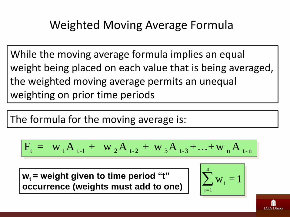
Weighted Moving Average Formula

F = w A + w A + w A +...+w At 1 t-1 2 t-2 3 t-3 n t- n

w = 1ii=1

n

While the moving average formula implies an equal weight being placed on each value that is being averaged, the weighted moving average permits an unequal weighting on prior time periods

wt = weight given to time period “t”

occurrence (weights must add to one)

The formula for the moving average is:

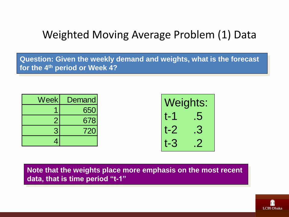
Weighted Moving Average Problem (1) Data

Weights:

t-1 .5

t-2 .3

t-3 .2

Week Demand

1 650

2 678

3 720

4

Question: Given the weekly demand and weights, what is the forecast

for the 4th period or Week 4?

Note that the weights place more emphasis on the most recent

data, that is time period “t-1”

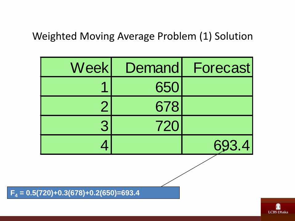
Weighted Moving Average Problem (1) Solution

Week Demand Forecast

1 650

2 678

3 720

4 693.4

F4 = 0.5(720)+0.3(678)+0.2(650)=693.4

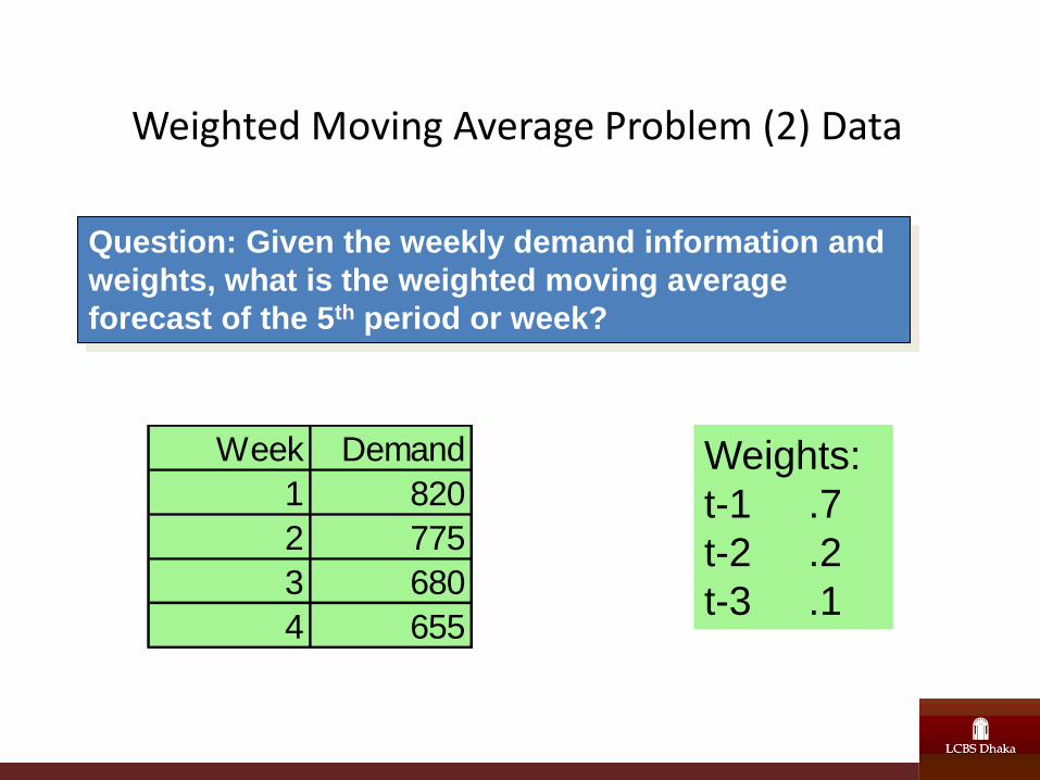
Weighted Moving Average Problem (2) Data

Weights:

t-1 .7

t-2 .2

t-3 .1

Week Demand

1 820

2 775

3 680

4 655

Question: Given the weekly demand information and

weights, what is the weighted moving average

forecast of the 5th period or week?

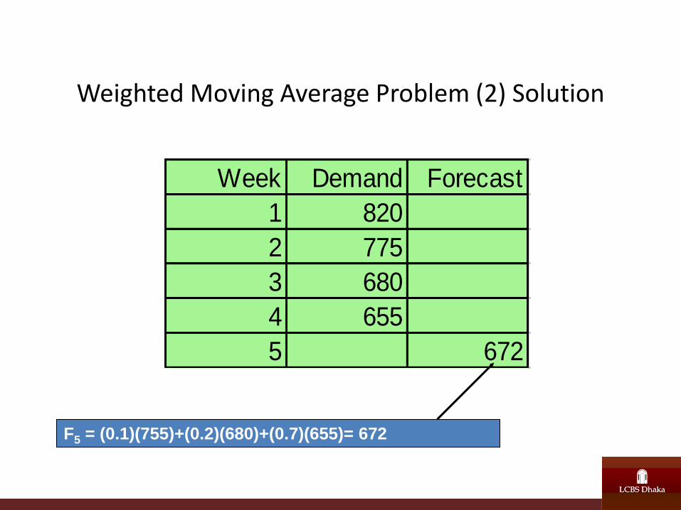
Weighted Moving Average Problem (2) Solution

Week Demand Forecast

1 820

2 775

3 680

4 655

5 672

F5 = (0.1)(755)+(0.2)(680)+(0.7)(655)= 672

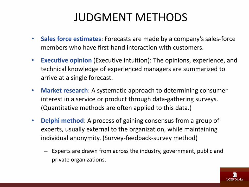
JUDGMENT METHODS

• Sales force estimates: Forecasts are made by a company’s sales-force

members who have first-hand interaction with customers.

• Executive opinion (Executive intuition): The opinions, experience, and technical knowledge of experienced managers are summarized to

arrive at a single forecast.

• Market research: A systematic approach to determining consumer interest in a service or product through data-gathering surveys.

(Quantitative methods are often applied to this data.)

• Delphi method: A process of gaining consensus from a group of experts, usually external to the organization, while maintaining

individual anonymity. (Survey-feedback-survey method)

– Experts are drawn from across the industry, government, public and

private organizations.

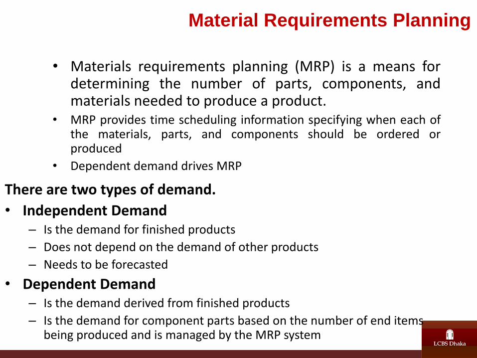
Material Requirements Planning

• Materials requirements planning (MRP) is a means for determining the number of parts, components, and materials needed to produce a product.

• MRP provides time scheduling information specifying when each of the materials, parts, and components should be ordered or produced

• Dependent demand drives MRP

There are two types of demand.

• Independent Demand – Is the demand for finished products

– Does not depend on the demand of other products

– Needs to be forecasted

• Dependent Demand – Is the demand derived from finished products

– Is the demand for component parts based on the number of end items being produced and is managed by the MRP system

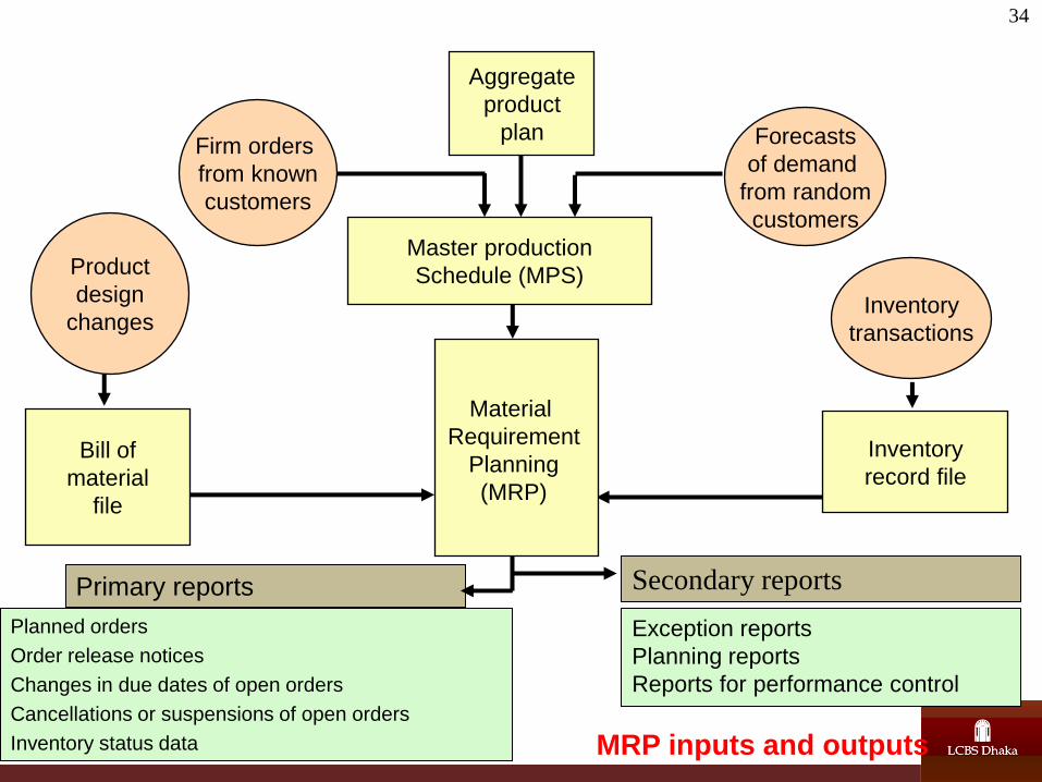
34

Firm orders

from known

customers

Forecasts

of demand

from random

customers

Aggregate

product

plan

Bill of

material

file

Product

design

changes

Inventory

record file

Inventory

transactions

Master production

Schedule (MPS)

Primary reports Secondary reports

Planned orders

Order release notices

Changes in due dates of open orders

Cancellations or suspensions of open orders

Inventory status data

Exception reports

Planning reports

Reports for performance control

Material

Requirement

Planning

(MRP)

MRP inputs and outputs

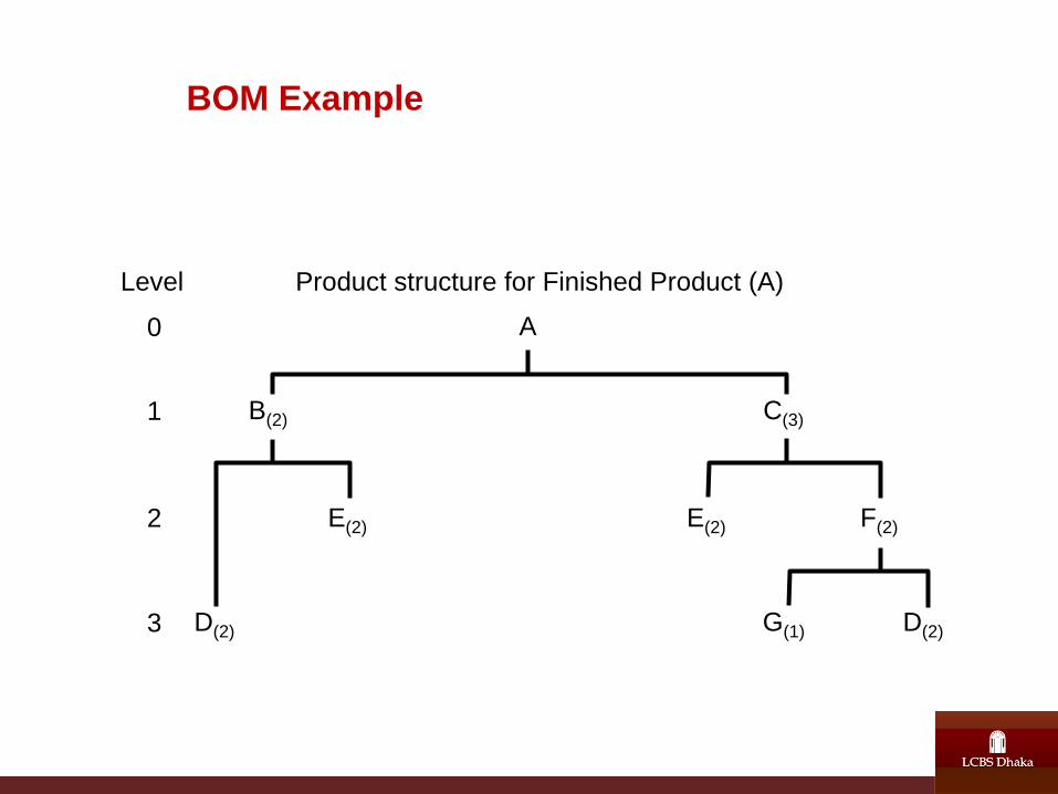
BOM Example

B(2) C(3) 1

E(2) E(2) F(2) 2

D(2) D(2) G(1) 3

Product structure for Finished Product (A)

A

Level

0

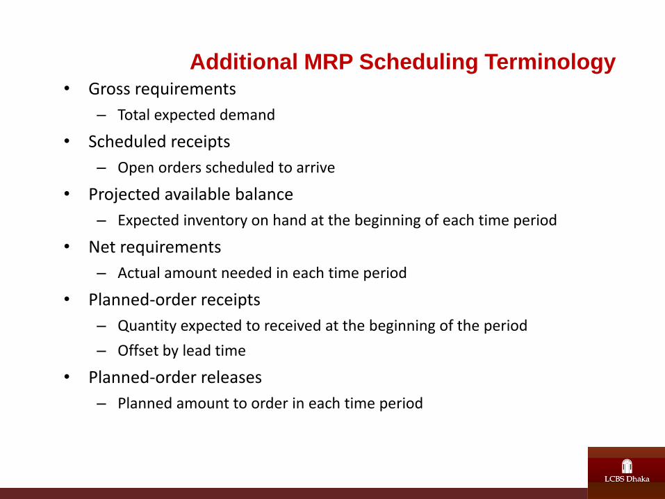
• Gross requirements

– Total expected demand

• Scheduled receipts

– Open orders scheduled to arrive

• Projected available balance

– Expected inventory on hand at the beginning of each time period

• Net requirements

– Actual amount needed in each time period

• Planned-order receipts

– Quantity expected to received at the beginning of the period

– Offset by lead time

• Planned-order releases

– Planned amount to order in each time period

Additional MRP Scheduling Terminology

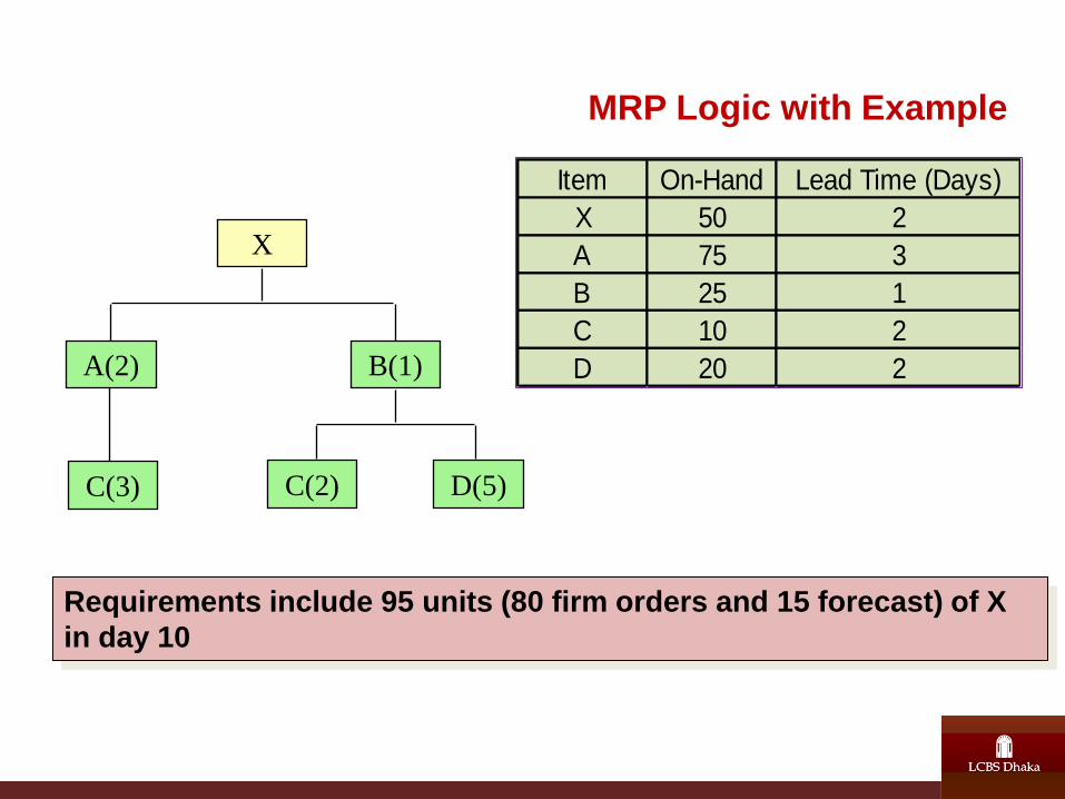
MRP Logic with Example

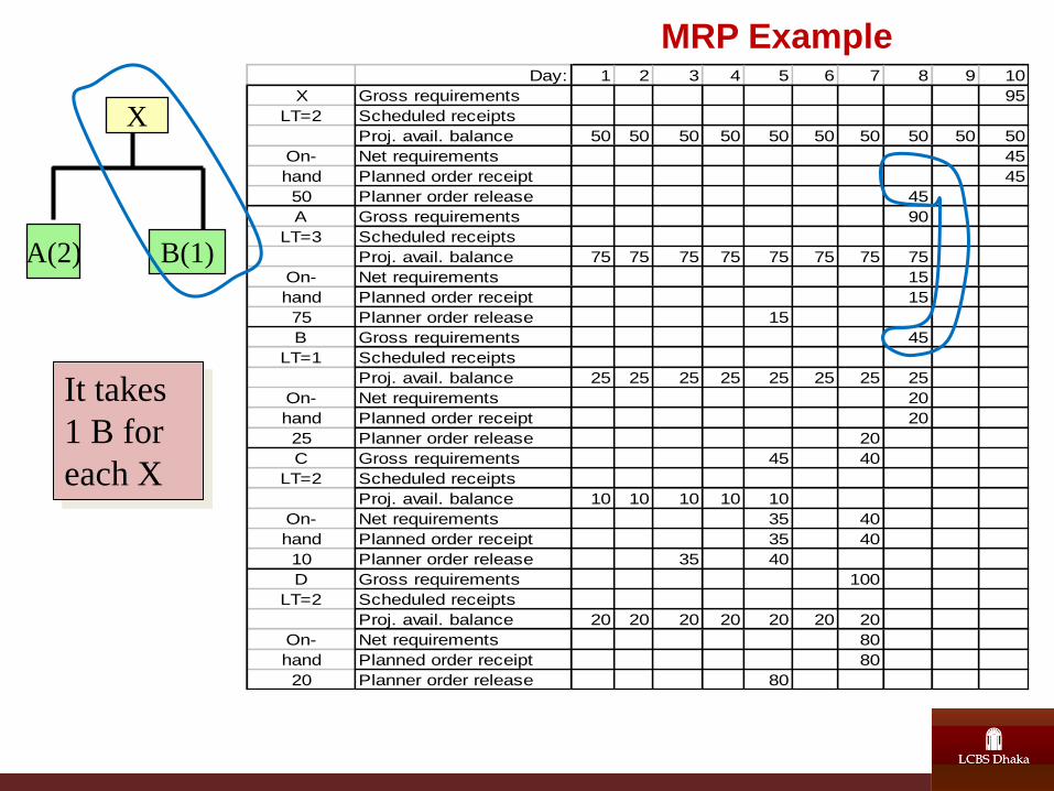
A(2) B(1)

D(5) C(2)

X

C(3)

Item On-Hand Lead Time (Days)

X 50 2

A 75 3

B 25 1

C 10 2

D 20 2

Requirements include 95 units (80 firm orders and 15 forecast) of X

in day 10

MRP Example 1 Day: 1 2 3 4 5 6 7 8 9 10

X Gross requirements

LT=2 Scheduled receipts

Proj. avail. balance

On- Net requirements

hand Planned order receipt

50 Planner order release

A Gross requirements






B Gross requirements






C Gross requirements






D Gross requirements






Item On-Hand Lead Time (Days)

X 50 2

A 75 3

B 25 1

C 10 2

D 20 2

Gross

requirement of X

is 95 units on

day 10

A(2) B(1)

D(5) C(2)

X

C(3)

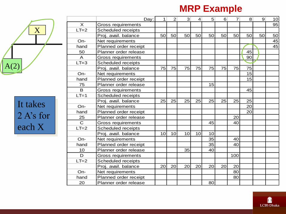
MRP Example Day: 1 2 3 4 5 6 7 8 9 10

X Gross requirements 95


Proj. avail. balance 50 50 50 50 50 50 50 50 50 50

On- Net requirements 45

hand Planned order receipt 45

50 Planner order release 45

A Gross requirements 90


Proj. avail. balance 75 75 75 75 75 75 75 75




B Gross requirements 45






C Gross requirements 45 40


Proj. avail. balance 10 10 10 10 10

On- Net requirements 35 40

hand Planned order receipt 35 40

10 Planner order release 35 40

D Gross requirements 100


Proj. avail. balance 20 20 20 20 20 20 20




X

It takes

2 A’s for

each X

A(2)

MRP Example Day: 1 2 3 4 5 6 7 8 9 10































X

It takes

1 B for

each X

A(2) B(1)

MRP Example Day: 1 2 3 4 5 6 7 8 9 10































X

It takes

3 C’s for

each A

A(2) B(1)

C(3)

MRP Example Day: 1 2 3 4 5 6 7 8 9 10































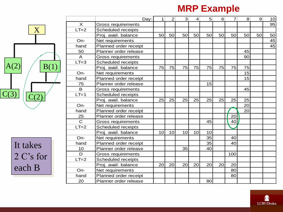
X

It takes

2 C’s for

each B

A(2) B(1)

C(3) C(2)

MRP Example Day: 1 2 3 4 5 6 7 8 9 10































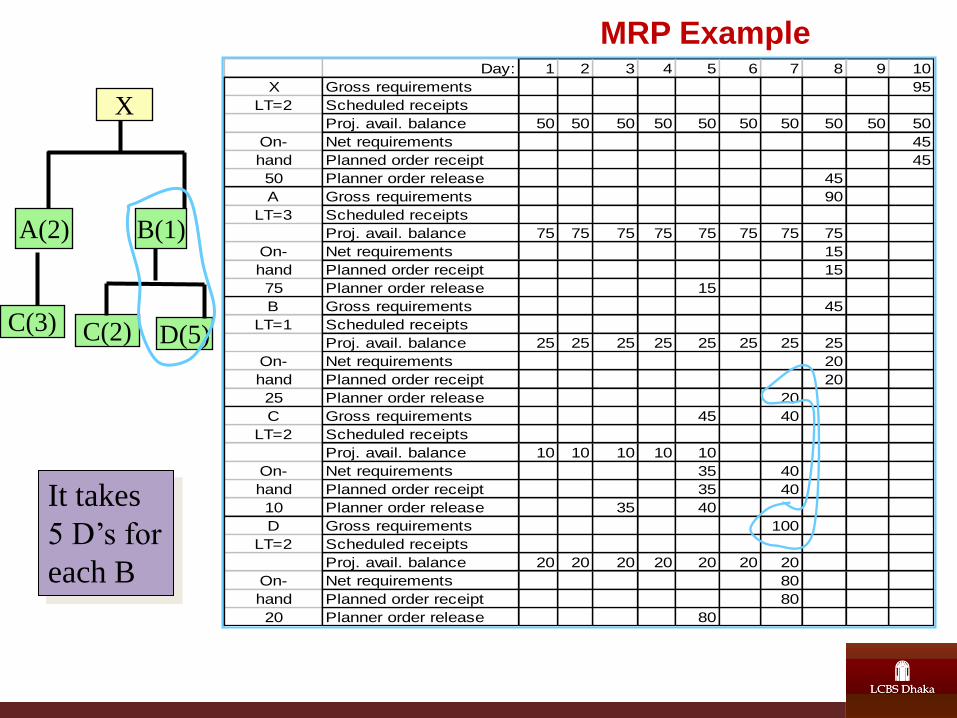
X

It takes

5 D’s for

each B

A(2) B(1)

C(3) C(2) D(5)

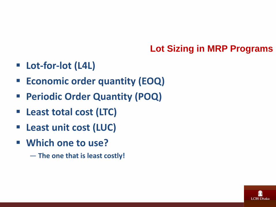
Lot Sizing in MRP Programs

Lot-for-lot (L4L)

Economic order quantity (EOQ)

Periodic Order Quantity (POQ)

Least total cost (LTC)

Least unit cost (LUC)

Which one to use? — The one that is least costly!

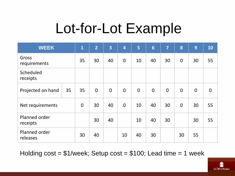
Lot-for-Lot Example WEEK 1 2 3 4 5 6 7 8 9 10

Gross requirements

35 30 40 0 10 40 30 0 30 55

Scheduled receipts

Projected on hand 35 35 0 0 0 0 0 0 0 0 0

Net requirements 0 30 40 0 10 40 30 0 30 55

Planned order receipts

30 40 10 40 30 30 55

Planned order releases

30 40 10 40 30 30 55

Holding cost = $1/week; Setup cost = $100; Lead time = 1 week

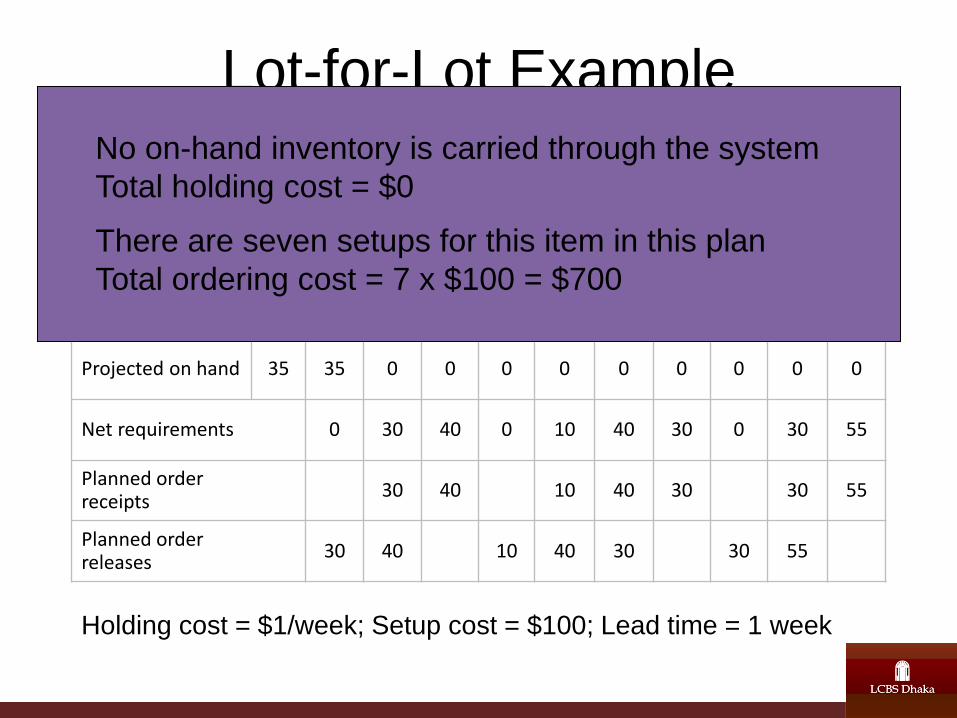
Lot-for-Lot Example

WEEK 1 2 3 4 5 6 7 8 9 10

Gross requirements

35 30 40 0 10 40 30 0 30 55

Scheduled receipts




30 40 10 40 30 30 55


30 40 10 40 30 30 55


No on-hand inventory is carried through the system

Total holding cost = $0

There are seven setups for this item in this plan

Total ordering cost = 7 x $100 = $700

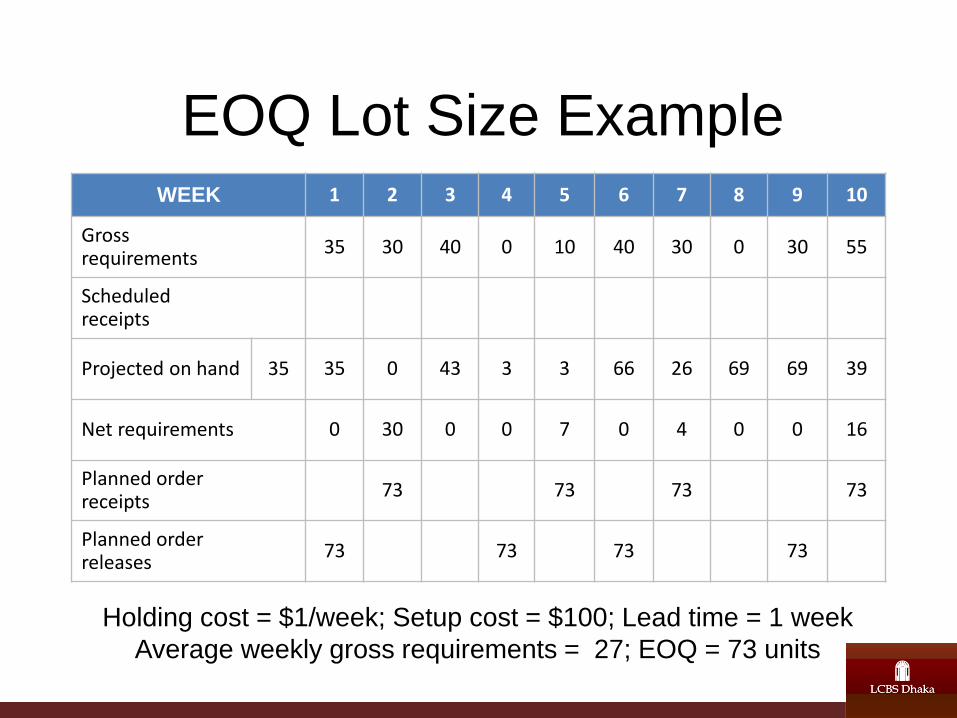
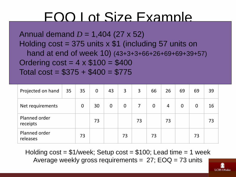
EOQ Lot Size Example WEEK 1 2 3 4 5 6 7 8 9 10

Gross requirements

35 30 40 0 10 40 30 0 30 55

Scheduled receipts




73 73 73 73


73 73 73 73


Average weekly gross requirements = 27; EOQ = 73 units

EOQ Lot Size Example

WEEK 1 2 3 4 5 6 7 8 9 10

Gross requirements

35 30 40 0 10 40 30 0 30 55

Scheduled receipts




73 73 73 73


73 73 73 73

Annual demand D = 1,404 (27 x 52)

Holding cost = 375 units x $1 (including 57 units on

hand at end of week 10) (43+3+3+66+26+69+69+39+57)

Ordering cost = 4 x $100 = $400

Total cost = $375 + $400 = $775


Average weekly gross requirements = 27; EOQ = 73 units

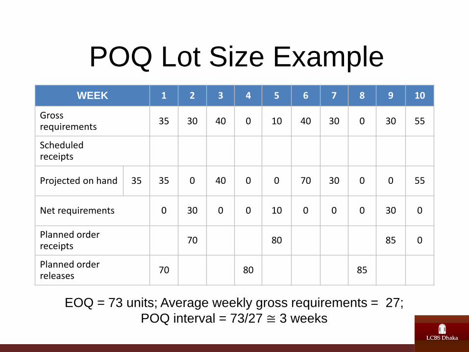
POQ Lot Size Example WEEK 1 2 3 4 5 6 7 8 9 10

Gross requirements

35 30 40 0 10 40 30 0 30 55

Scheduled receipts




70 80 85 0


70 80 85

EOQ = 73 units; Average weekly gross requirements = 27;

POQ interval = 73/27 ≅ 3 weeks

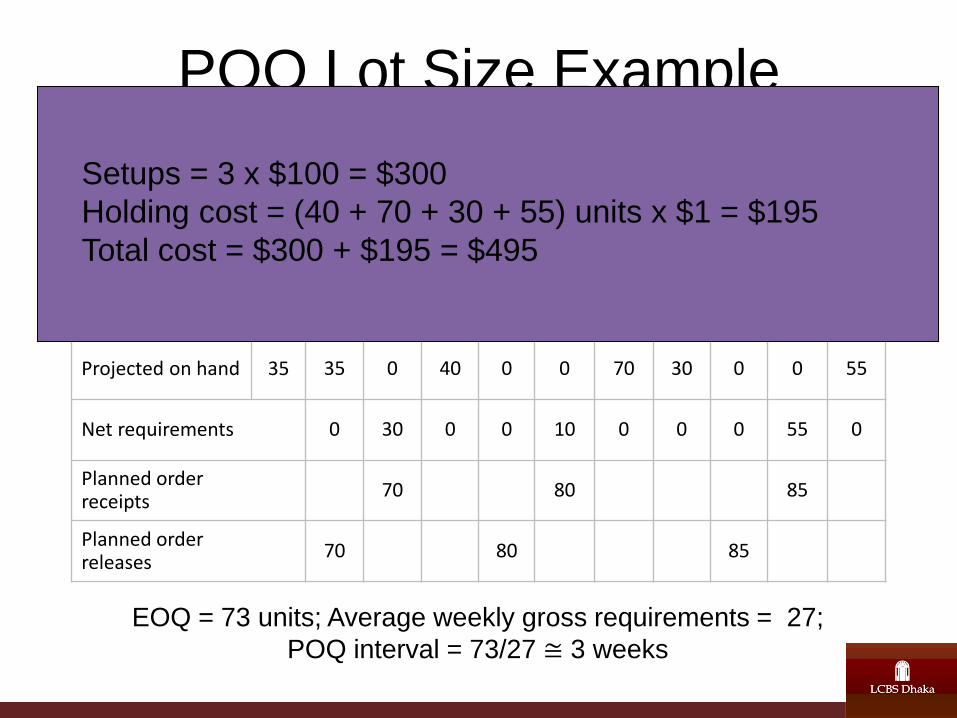
POQ Lot Size Example

WEEK 1 2 3 4 5 6 7 8 9 10

Gross requirements

35 30 40 0 10 40 30 0 30 55

Scheduled receipts




70 80 85


70 80 85

Setups = 3 x $100 = $300

Holding cost = (40 + 70 + 30 + 55) units x $1 = $195

Total cost = $300 + $195 = $495

EOQ = 73 units; Average weekly gross requirements = 27;

POQ interval = 73/27 ≅ 3 weeks

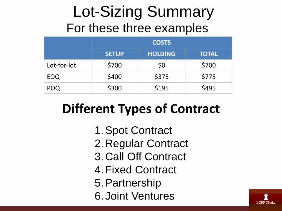
Lot-Sizing Summary For these three examples

COSTS

SETUP HOLDING TOTAL

Lot-for-lot $700 $0 $700

EOQ $400 $375 $775

POQ $300 $195 $495

1.Spot Contract

2.Regular Contract

3.Call Off Contract

4.Fixed Contract

5.Partnership

6.Joint Ventures

Different Types of Contract

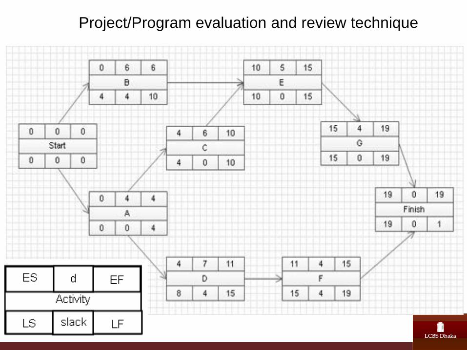
Project/Program evaluation and review technique

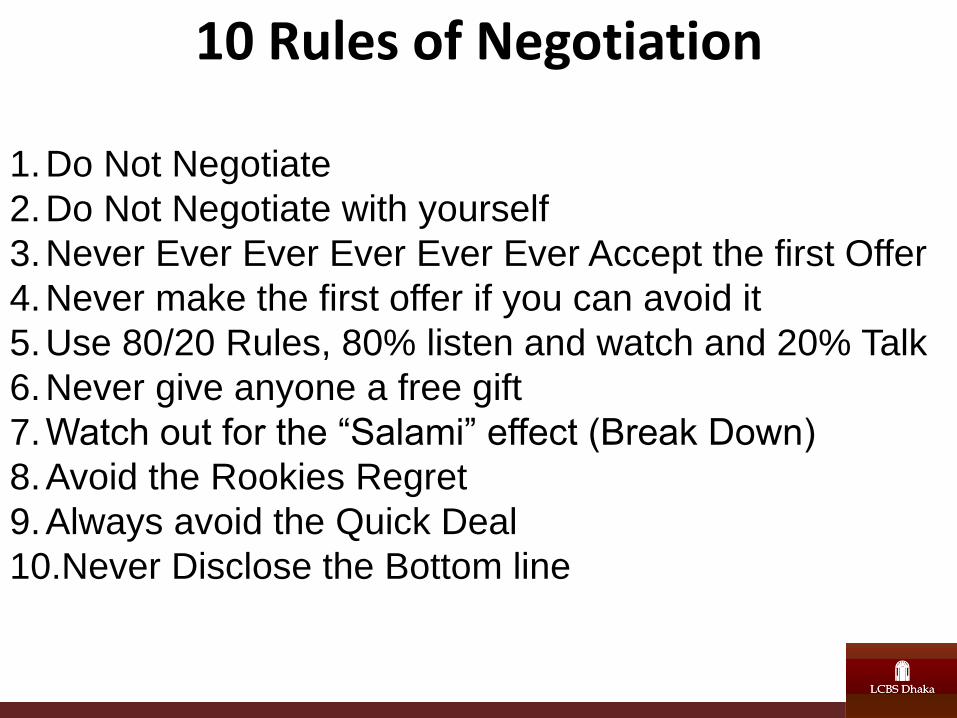
10 Rules of Negotiation 1.Do Not Negotiate

2.Do Not Negotiate with yourself

3.Never Ever Ever Ever Ever Ever Accept the first Offer

4.Never make the first offer if you can avoid it

5.Use 80/20 Rules, 80% listen and watch and 20% Talk

6.Never give anyone a free gift

7.Watch out for the “Salami” effect (Break Down)

8.Avoid the Rookies Regret

9.Always avoid the Quick Deal

10.Never Disclose the Bottom line

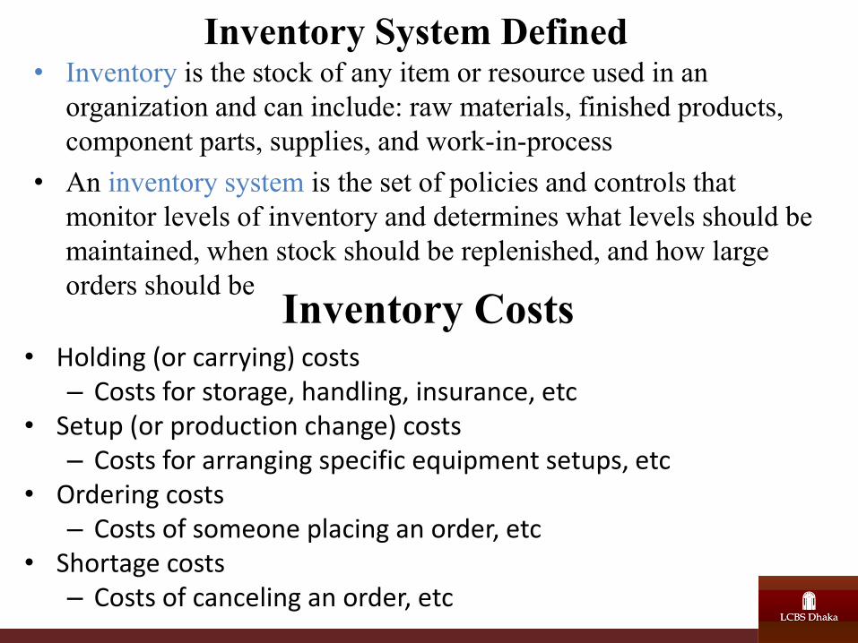
Inventory System Defined • Inventory is the stock of any item or resource used in an

organization and can include: raw materials, finished products,

component parts, supplies, and work-in-process

• An inventory system is the set of policies and controls that

monitor levels of inventory and determines what levels should be

maintained, when stock should be replenished, and how large

orders should be Inventory Costs

• Holding (or carrying) costs – Costs for storage, handling, insurance, etc

• Setup (or production change) costs – Costs for arranging specific equipment setups, etc

• Ordering costs – Costs of someone placing an order, etc

• Shortage costs – Costs of canceling an order, etc

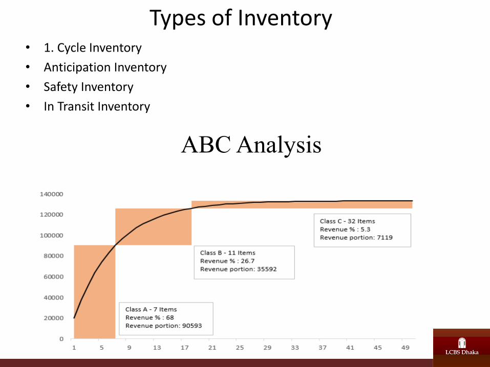
Types of Inventory • 1. Cycle Inventory

• Anticipation Inventory

• Safety Inventory

• In Transit Inventory

ABC Analysis

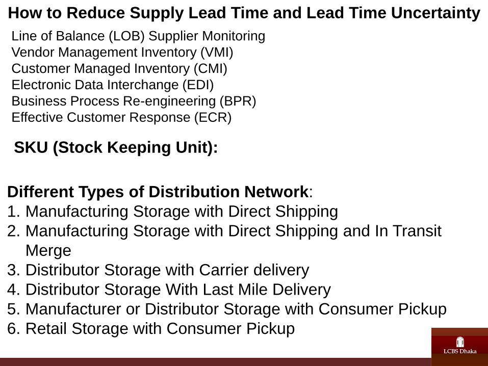
How to Reduce Supply Lead Time and Lead Time Uncertainty

Line of Balance (LOB) Supplier Monitoring

Vendor Management Inventory (VMI)

Customer Managed Inventory (CMI)

Electronic Data Interchange (EDI)

Business Process Re-engineering (BPR)

Effective Customer Response (ECR)

SKU (Stock Keeping Unit):

Different Types of Distribution Network:

1. Manufacturing Storage with Direct Shipping

2. Manufacturing Storage with Direct Shipping and In Transit

Merge

3. Distributor Storage with Carrier delivery

4. Distributor Storage With Last Mile Delivery

5. Manufacturer or Distributor Storage with Consumer Pickup

6. Retail Storage with Consumer Pickup

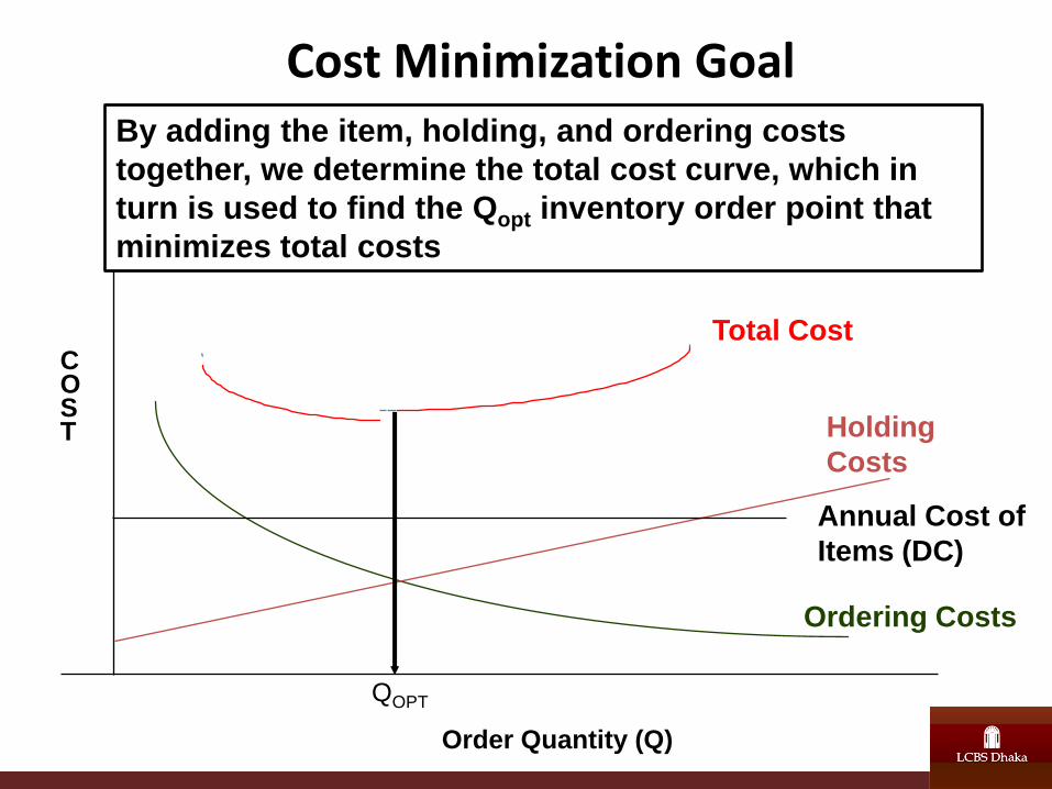
Cost Minimization Goal

Ordering Costs

Holding

Costs

Order Quantity (Q)

C O S T

Annual Cost of

Items (DC)

Total Cost

QOPT

By adding the item, holding, and ordering costs

together, we determine the total cost curve, which in

turn is used to find the Qopt inventory order point that

minimizes total costs

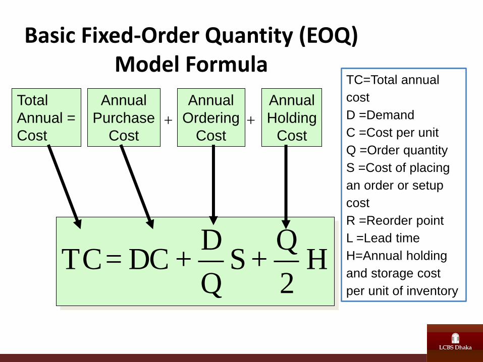
Basic Fixed-Order Quantity (EOQ) Model Formula

H 2

Q + S

Q

D + DC = TC

Total

Annual =

Cost

Annual

Purchase

Cost

Annual

Ordering

Cost

Annual

Holding

Cost + +

TC=Total annual

cost

D =Demand

C =Cost per unit

Q =Order quantity

S =Cost of placing

an order or setup

cost

R =Reorder point

L =Lead time

H=Annual holding

and storage cost

per unit of inventory

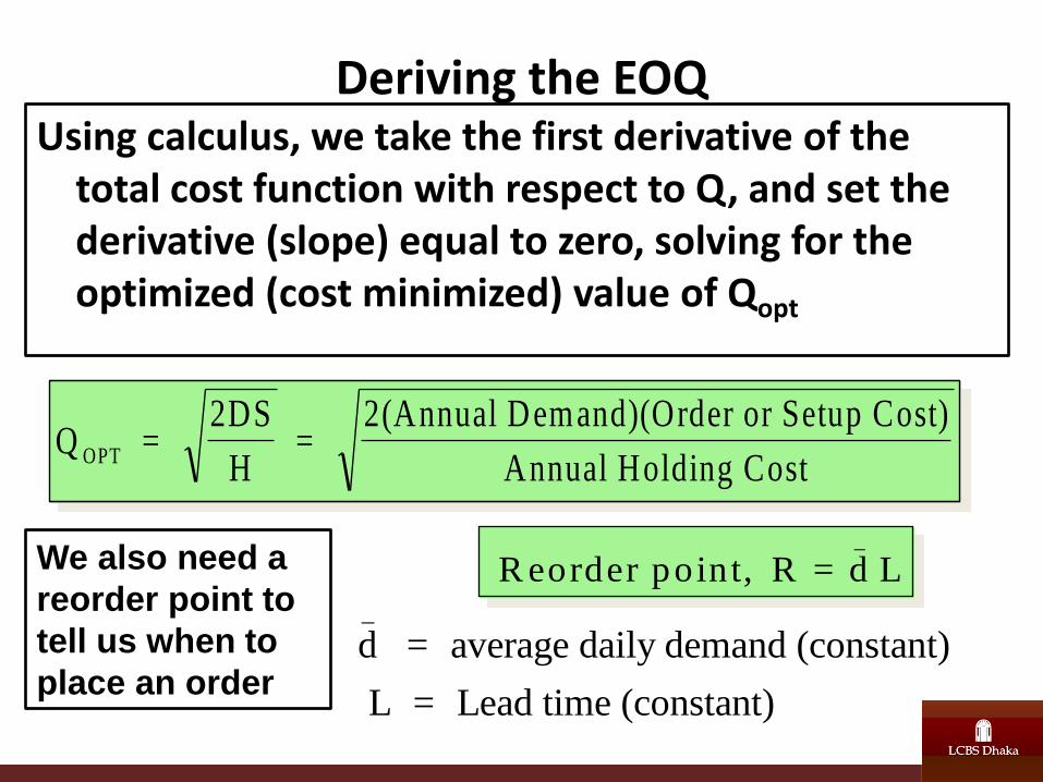
Deriving the EOQ Using calculus, we take the first derivative of the

total cost function with respect to Q, and set the derivative (slope) equal to zero, solving for the optimized (cost minimized) value of Qopt

Q = 2DS

H =

2(Annual Demand)(Order or Setup Cost)

Annual Holding CostOPT

R eorder point, R = d L_

d = average daily demand (constant)

L = Lead time (constant)

_

We also need a

reorder point to

tell us when to

place an order

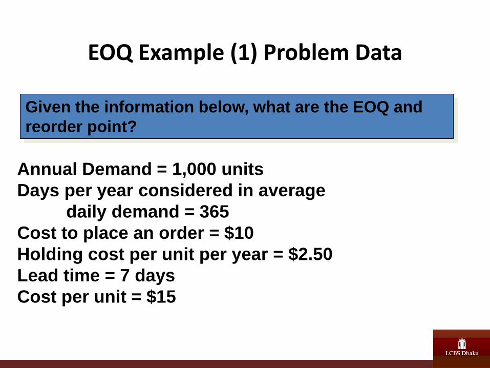
EOQ Example (1) Problem Data

Annual Demand = 1,000 units

Days per year considered in average

daily demand = 365

Cost to place an order = $10

Holding cost per unit per year = $2.50

Lead time = 7 days

Cost per unit = $15

Given the information below, what are the EOQ and

reorder point?

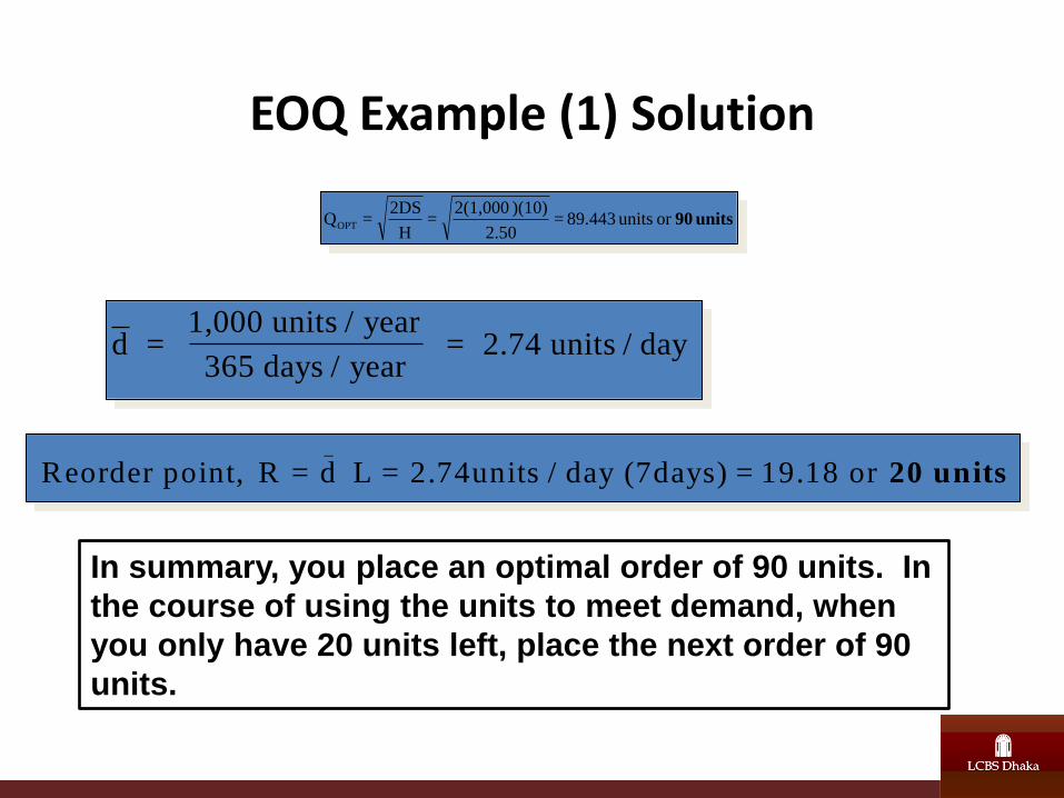
EOQ Example (1) Solution

units 90or units 89.443 = 2.50

)(10) 2(1,000 =

H

2DS = QOPT

d = 1,000 units / year

365 days / year = 2.74 units / day

Reorder point, R = d L = 2.74units / day (7days) = 19.18 or _

20 units

In summary, you place an optimal order of 90 units. In

the course of using the units to meet demand, when

you only have 20 units left, place the next order of 90

units.

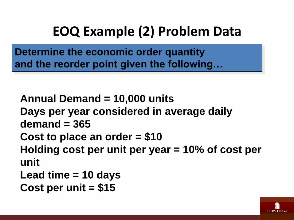
EOQ Example (2) Problem Data

Annual Demand = 10,000 units

Days per year considered in average daily

demand = 365

Cost to place an order = $10

Holding cost per unit per year = 10% of cost per

unit

Lead time = 10 days

Cost per unit = $15

Determine the economic order quantity

and the reorder point given the following…

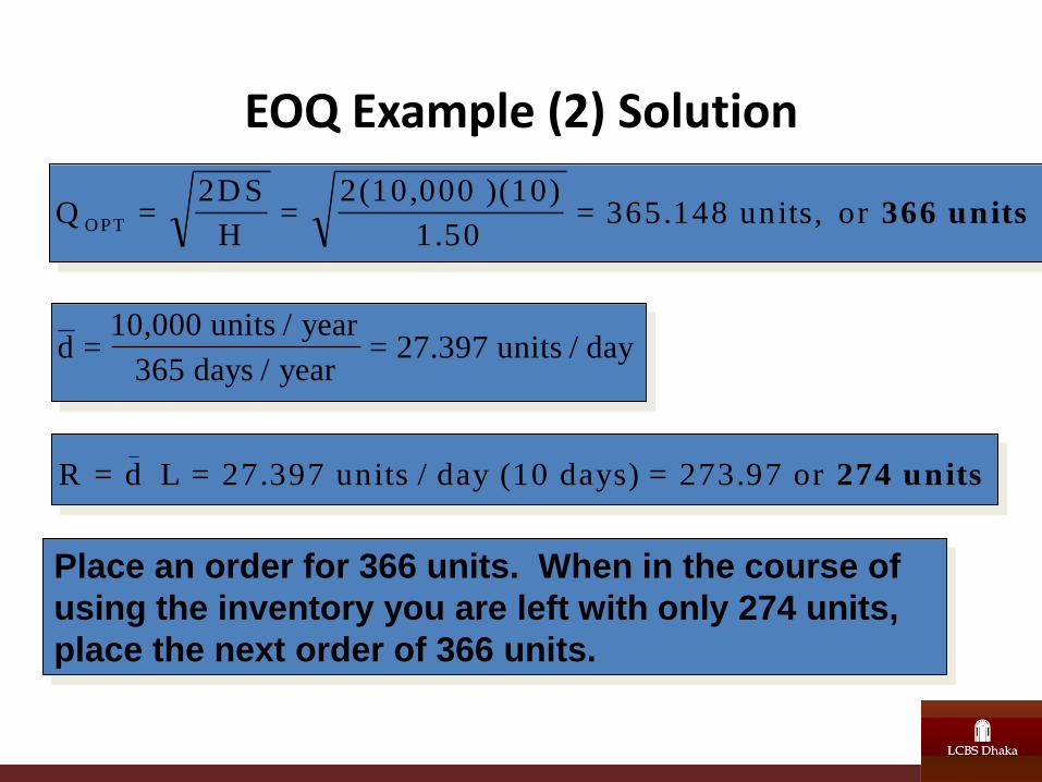
EOQ Example (2) Solution

Q =2D S

H=

2(10,000 )(10)

1.50= 365.148 units, or O PT 366 units

d =10,000 units / year

365 days / year= 27.397 units / day

R = d L = 27.397 units / day (10 days) = 273.97 or _

274 units

Place an order for 366 units. When in the course of

using the inventory you are left with only 274 units,

place the next order of 366 units.

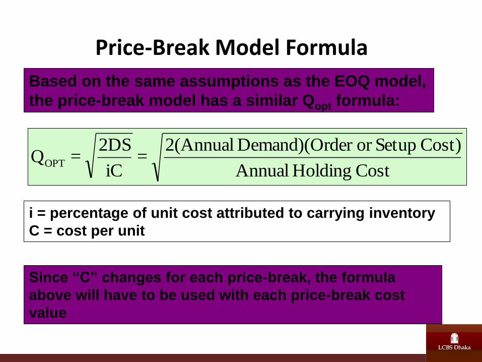
Price-Break Model Formula

Cost Holding Annual

Cost) Setupor der Demand)(Or 2(Annual =

iC

2DS = QOPT

Based on the same assumptions as the EOQ model,

the price-break model has a similar Qopt formula:

i = percentage of unit cost attributed to carrying inventory

C = cost per unit

Since “C” changes for each price-break, the formula

above will have to be used with each price-break cost

value

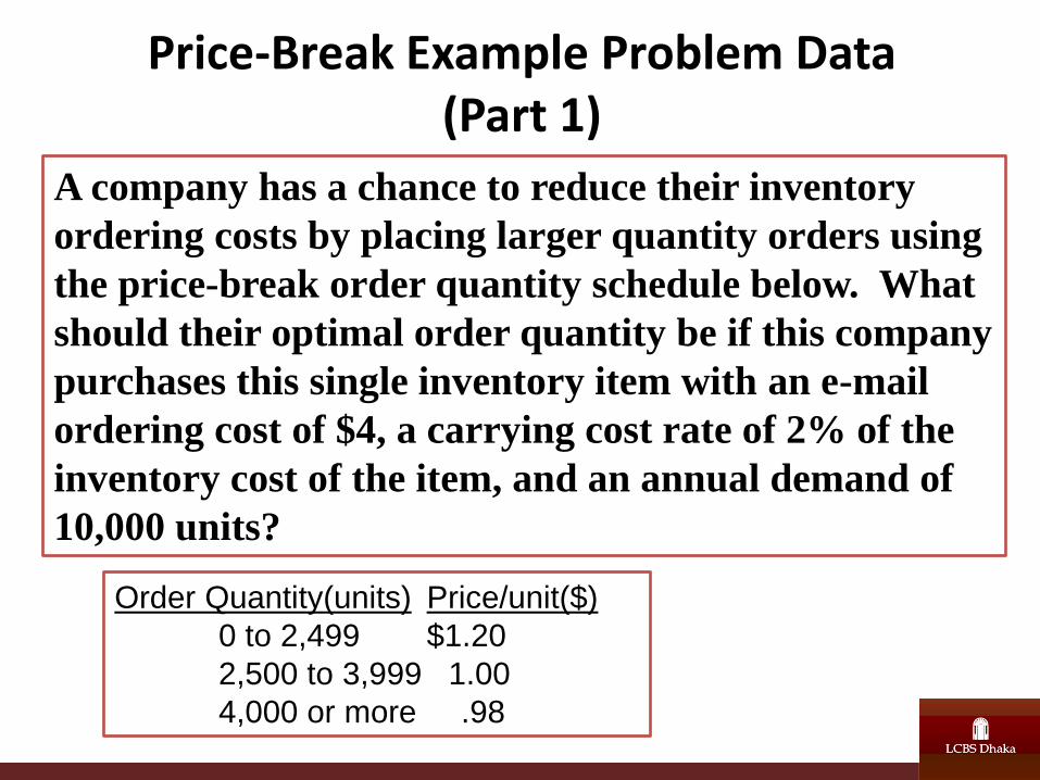
Price-Break Example Problem Data (Part 1)

A company has a chance to reduce their inventory

ordering costs by placing larger quantity orders using

the price-break order quantity schedule below. What

should their optimal order quantity be if this company

purchases this single inventory item with an e-mail

ordering cost of $4, a carrying cost rate of 2% of the

inventory cost of the item, and an annual demand of

10,000 units?

Order Quantity(units) Price/unit($)

0 to 2,499 $1.20

2,500 to 3,999 1.00

4,000 or more .98

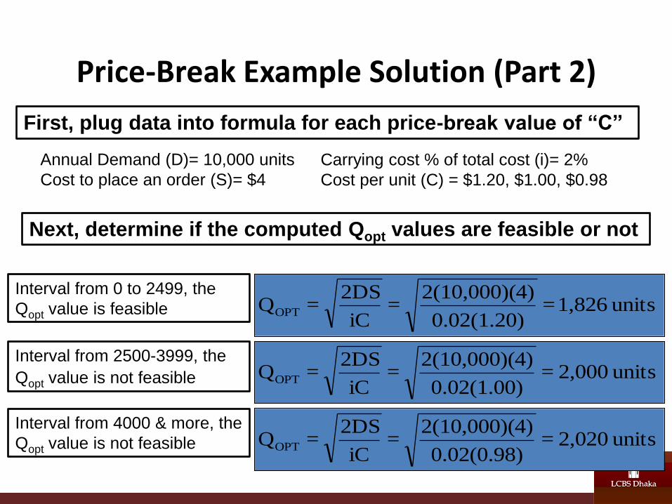
Price-Break Example Solution (Part 2)

units 1,826 = 0.02(1.20)

4)2(10,000)( =

iC

2DS = QOPT

Annual Demand (D)= 10,000 units

Cost to place an order (S)= $4

First, plug data into formula for each price-break value of “C”

units 2,000 = 0.02(1.00)

4)2(10,000)( =

iC

2DS = QOPT

units 2,020 = 0.02(0.98)

4)2(10,000)( =

iC

2DS = QOPT

Carrying cost % of total cost (i)= 2%

Cost per unit (C) = $1.20, $1.00, $0.98

Interval from 0 to 2499, the

Qopt value is feasible

Interval from 2500-3999, the

Qopt value is not feasible

Interval from 4000 & more, the

Qopt value is not feasible

Next, determine if the computed Qopt values are feasible or not

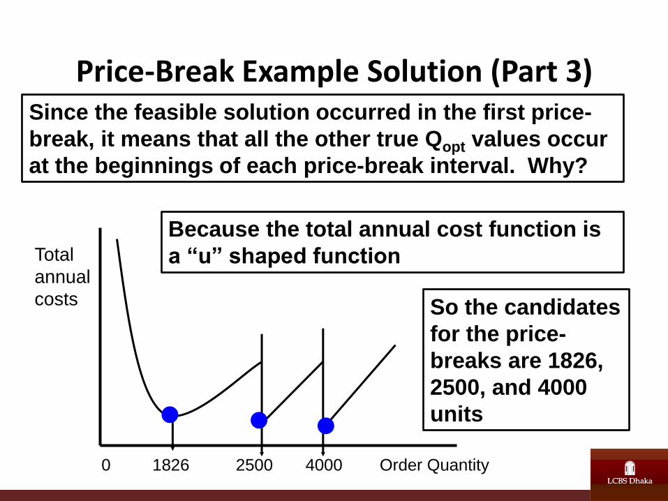
Price-Break Example Solution (Part 3) Since the feasible solution occurred in the first price-

break, it means that all the other true Qopt values occur

at the beginnings of each price-break interval. Why?

0 1826 2500 4000 Order Quantity

Total

annual

costs So the candidates

for the price-

breaks are 1826,

2500, and 4000

units

Because the total annual cost function is

a “u” shaped function

Price-Break Example Solution (Part 4)

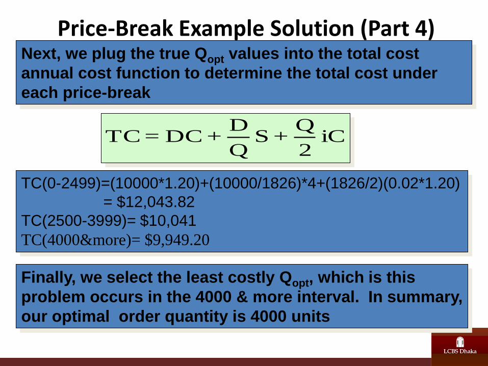
iC 2

Q + S

Q

D + DC = TC

Next, we plug the true Qopt values into the total cost

annual cost function to determine the total cost under

each price-break

TC(0-2499)=(10000*1.20)+(10000/1826)*4+(1826/2)(0.02*1.20)

= $12,043.82

TC(2500-3999)= $10,041

TC(4000&more)= $9,949.20

Finally, we select the least costly Qopt, which is this

problem occurs in the 4000 & more interval. In summary,

our optimal order quantity is 4000 units

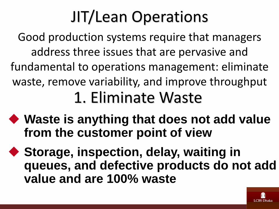
JIT/Lean Operations Good production systems require that managers

address three issues that are pervasive and fundamental to operations management: eliminate waste, remove variability, and improve throughput

Waste is anything that does not add value from the customer point of view

Storage, inspection, delay, waiting in queues, and defective products do not add value and are 100% waste

1. Eliminate Waste

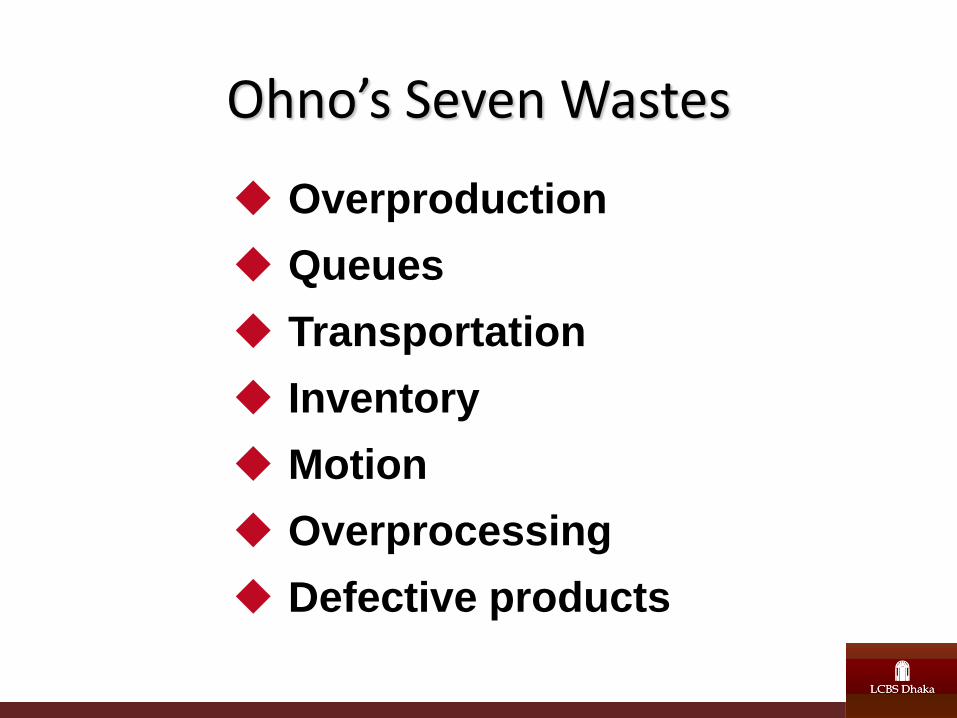
Ohno’s Seven Wastes

Overproduction

Queues

Transportation

Inventory

Motion

Overprocessing

Defective products

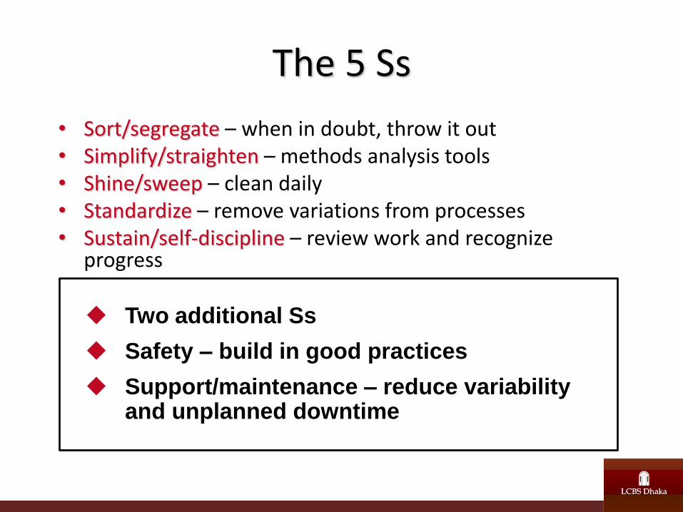
The 5 Ss

• Sort/segregate – when in doubt, throw it out • Simplify/straighten – methods analysis tools • Shine/sweep – clean daily • Standardize – remove variations from processes • Sustain/self-discipline – review work and recognize

progress

Two additional Ss

Safety – build in good practices

Support/maintenance – reduce variability and unplanned downtime

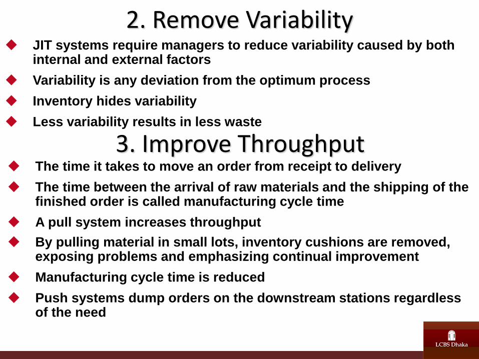
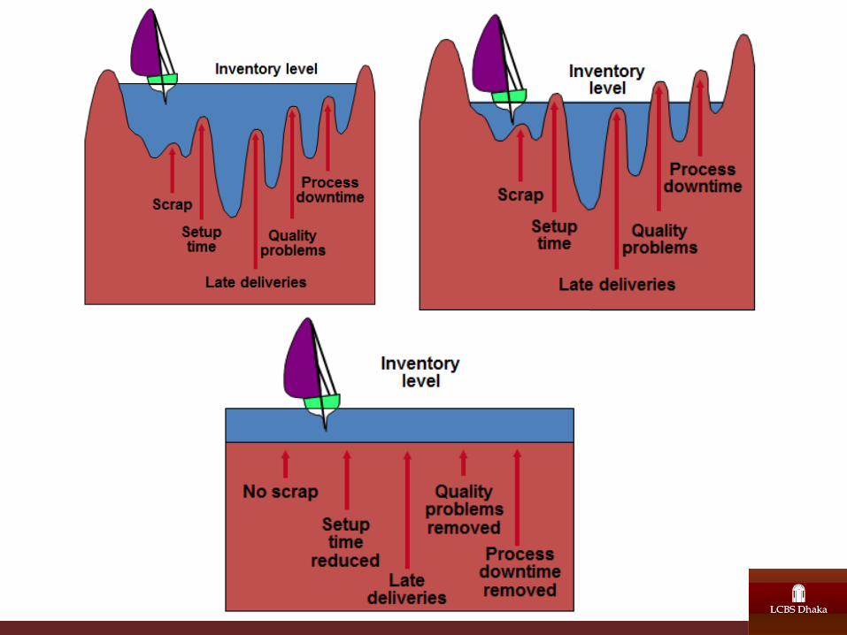
2. Remove Variability JIT systems require managers to reduce variability caused by both

internal and external factors

Variability is any deviation from the optimum process

Inventory hides variability

Less variability results in less waste

3. Improve Throughput The time it takes to move an order from receipt to delivery

The time between the arrival of raw materials and the shipping of the finished order is called manufacturing cycle time

A pull system increases throughput

By pulling material in small lots, inventory cushions are removed, exposing problems and emphasizing continual improvement

Manufacturing cycle time is reduced

Push systems dump orders on the downstream stations regardless of the need

Why Six Sigma?

Visible costs •Scrap

•Rework

•Warranty

Hidden Costs

• Conversion efficiency of materials

• Inadequate resource utilization

• Excessive use of material

• Cost of redesign and re-inspection

• Cost of resolving customer problems

• Lost customers / Goodwill

• High inventory

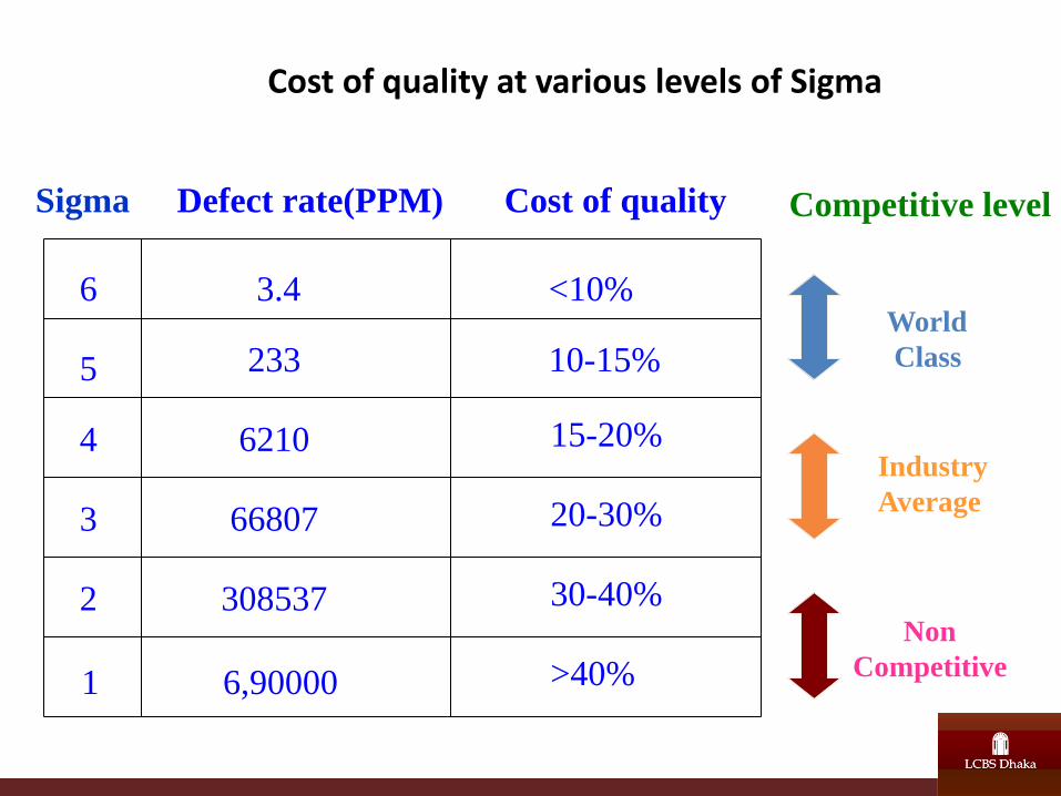
Cost of quality at various levels of Sigma

Sigma Defect rate(PPM) Cost of quality Competitive level

3.4 <10%

233 10-15%

6210 15-20%

66807 20-30%

308537 30-40%

6,90000 >40%

World

Class

Industry

Average

Non

Competitive

6

5

4

3

2

1

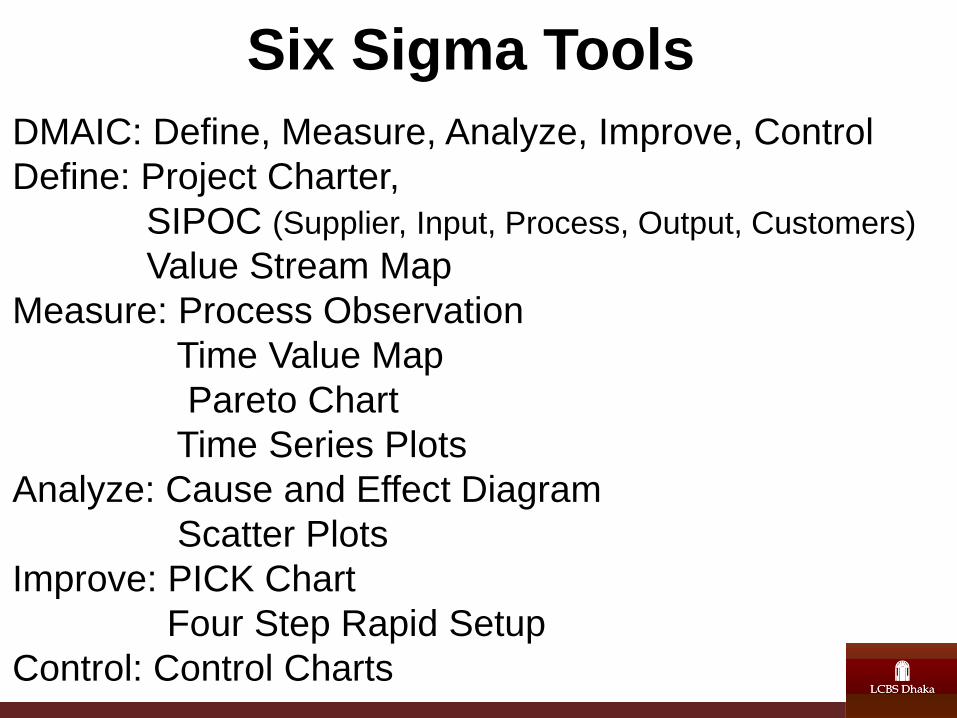
DMAIC: Define, Measure, Analyze, Improve, Control

Define: Project Charter,

SIPOC (Supplier, Input, Process, Output, Customers)

Value Stream Map

Measure: Process Observation

Time Value Map

Pareto Chart

Time Series Plots

Analyze: Cause and Effect Diagram

Scatter Plots

Improve: PICK Chart

Four Step Rapid Setup

Control: Control Charts

Six Sigma Tools

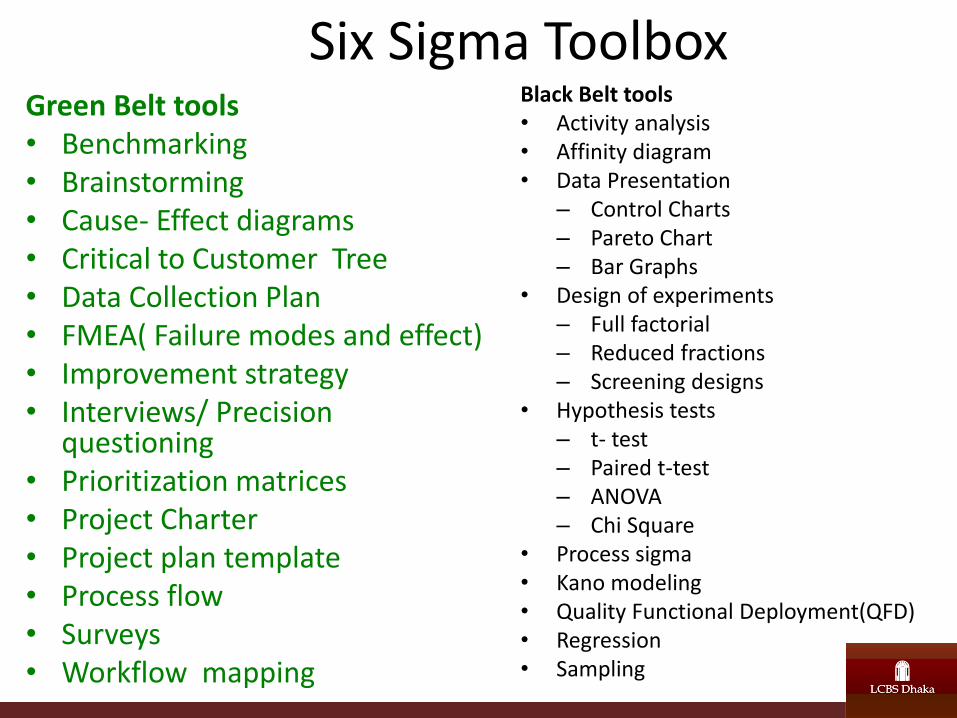
Six Sigma Toolbox Green Belt tools • Benchmarking • Brainstorming • Cause- Effect diagrams • Critical to Customer Tree • Data Collection Plan • FMEA( Failure modes and effect) • Improvement strategy • Interviews/ Precision

questioning • Prioritization matrices • Project Charter • Project plan template • Process flow • Surveys • Workflow mapping

Black Belt tools • Activity analysis • Affinity diagram • Data Presentation

– Control Charts – Pareto Chart – Bar Graphs

• Design of experiments – Full factorial – Reduced fractions – Screening designs

• Hypothesis tests – t- test – Paired t-test – ANOVA – Chi Square

• Process sigma • Kano modeling • Quality Functional Deployment(QFD) • Regression • Sampling

Documents

Mat and Inventory