Matching Natural Language Sentenceswith Hierarchical Sentence Factorization

Bang Liu1, Ting Zhang1, Fred X. Han1, Di Niu1, Kunfeng Lai2, Yu Xu21University of Alberta, Edmonton, AB, Canada

2Mobile Internet Group, Tencent, Shenzhen, China

ABSTRACTSemantic matching of natural language sentences or identifyingthe relationship between two sentences is a core research problemunderlying many natural language tasks. Depending on whethertraining data is available, prior research has proposed both un-supervised distance-based schemes and supervised deep learningschemes for sentence matching. However, previous approaches ei-ther omit or fail to fully utilize the ordered, hierarchical, and flexiblestructures of language objects, as well as the interactions betweenthem. In this paper, we propose Hierarchical Sentence Factorization—a technique to factorize a sentence into a hierarchical representa-tion, with the components at each different scale reordered into a“predicate-argument” form. The proposed sentence factorizationtechnique leads to the invention of: 1) a new unsupervised distancemetric which calculates the semantic distance between a pair of textsnippets by solving a penalized optimal transport problem whilepreserving the logical relationship of words in the reordered sen-tences, and 2) new multi-scale deep learning models for supervisedsemantic training, based on factorized sentence hierarchies. Weapply our techniques to text-pair similarity estimation and text-pairrelationship classification tasks, based on multiple datasets such asSTSbenchmark, the Microsoft Research paraphrase identification(MSRP) dataset, the SICK dataset, etc. Extensive experiments showthat the proposed hierarchical sentence factorization can be usedto significantly improve the performance of existing unsuperviseddistance-based metrics as well as multiple supervised deep learningmodels based on the convolutional neural network (CNN) and longshort-term memory (LSTM).

1 INTRODUCTIONSemantic matching, which aims to model the underlying semanticsimilarity or dissimilarity among different textual elements suchas sentences and documents, has been playing a central role inmany Natural Language Processing (NLP) applications, includinginformation extraction [14], top-k re-ranking in machine transla-tion [8], question-answering [44], automatic text summarization[29]. However, semantic matching based on either supervised orunsupervised learning remains a hard problem. Natural languagedemonstrates complicated hierarchical structures, where different

This paper is published under the Creative Commons Attribution 4.0 International(CC BY 4.0) license. Authors reserve their rights to disseminate the work on theirpersonal and corporate Web sites with the appropriate attribution. In case of republi-cation, reuse, etc., the following attribution should be used: “Published in WWW2018Proceedings © 2018 International World Wide Web Conference Committee, publishedunder Creative Commons CC BY 4.0 License.”WWW 2018, April 23–27, 2018, Lyon, France© 2018 IW3C2 (International World Wide Web Conference Committee), publishedunder Creative Commons CC BY 4.0 License.ACM ISBN 978-1-4503-5639-8.https://doi.org/10.1145/3178876.3186022

words can be organized in different orders to express the sameidea. As a result, appropriate semantic representation of text playsa critical role in matching natural language sentences.

Traditional approaches represent text objects as bag-of-words(BoW), term frequency inverse document frequency (TF-IDF) [43]vectors, or their enhanced variants [26, 32]. However, such represen-tations can not accurately capture the similarity between individualwords, and do not take the semantic structure of language into con-sideration. Alternatively, word embeddingmodels, such asword2vec[23] and Glove [28], learn a distributional semantic representationof each word and have been widely used.

Based on the word-vector representation, a number of unsuper-vised and supervised matching schemes have been recently pro-posed. As an unsupervised learning approach, the Word Mover’sDistance (WMD) metric [21] measures the dissimilarity betweentwo sentences (or documents) as the minimum distance to transportthe embedded words of one sentence to those of another sentence.However, the sequential and structural nature of sentences is omit-ted in WMD. For example, two sentences containing exactly thesame words in different orders can express totally different mean-ings. On the other hand, many supervised learning schemes basedon deep neural networks have also been proposed for sentencematching [24, 27, 35, 41]. A common characteristic of many of theseneural network models is that they adopt a Siamese architecture,taking the word embedding sequences of a pair of sentences (ordocuments) as the input, transforming them into intermediate con-textual representations via either convolutional or recurrent neuralnetworks, and performing scoring over the contextual representa-tions to yield final matching results. However, these methods relypurely on neural networks to learn the complicated relationshipsamong sentences, andmany obvious compositional and hierarchicalfeatures are often overlooked or not explicitly utilized.

In this paper, however, we argue that a successful semanticmatching algorithm needs to best characterize the sequential, hi-erarchical and flexible structure of natural language sentences, aswell as the rich interaction patterns among semantic units. Wepresent a technique named Hierarchical Sentence Factorization (orSentence Factorization in short), which is able to represent a sen-tence in a hierarchical semantic tree, with each node (semanticunit) at different depths of the tree reorganized into a normalized“predicate-argument” form. Such normalized sentence representa-tion enables us to propose new methods to both improve unsuper-vised semantic matching by taking the structural and sequentialdifferences between two text entities into account, and enhance arange of supervised semantic matching schemes, by overcomingthe limitation of the representation capability of convolutional orrecurrent neural networks, especially when labelled training datais limited. Specifically, we make the following contributions:

arX

iv:1

803.

0017

9v1

[cs

.CL

] 1

Mar

201

8

First, the proposed Sentence Factorization scheme factorizes a sen-tence recursively into a hierarchical tree of semantic units, whereeach unit is a subset of words from the original sentence. Words arethen reordered into a “predicate-argument” structure. Such form ofsentence representation offers two benefits: i) the flexible syntaxstructures of the same sentence, for example, active and passivesentences, can be normalized into a unified representation; ii) thesemantic units in a pair of sentences can be aligned according totheir depth and order in the factorization tree.

Second, for unsupervised text matching, we combine the fac-torized and reordered representation of sentences and the Order-preserving Wasserstein Distance [37] (which was originally pro-posed to match hand-written characters in computer vision) to pro-pose a new semantic distance metric between text objects, whichwe call Ordered Word Mover’s Distance. Compared with the recentlyproposed Word Mover’s Distance [21], our new metric achievessignificant improvement by taking the sequential structures of sen-tences into account. For example, without considering the order ofwords, the Word Mover’s Distance between the sentences “Tom ischasing Jerry” and “Jerry is chasing Tom” is zero. In contrast, ournew metric is able to penalize such order mismatch between words,and identify the difference between the two sentences.

Third, for supervised semantic matching, we extend the exist-ing Siamese network architectures (both for CNN and LSTM) tomulti-scaled models, where each scale adopts an individual Siamesenetwork, taking as input the vector representations of the two sen-tences at the corresponding depth in the factorization trees, rangingfrom the coarse-grained scale to fine-grained scales. When increas-ing the number of layers in the corresponding neural network canhardly improve performance, hierarchical sentence factorizationprovides a novel means to extend the original deep networks toa “richer” model that matches a pair of sentences through a multi-scaled semantic unit matching process. Our proposed multi-scaleddeep neural networks can effectively improve existing deep modelsby measuring the similarity between a pair of sentences at differ-ent semantic granularities. For instance, Siamese networks basedon CNN and BiLSTM [24, 36] that originally only take the wordsequences as the inputs.

We extensively evaluate the performance of our proposed ap-proaches on the task of semantic textual similarity estimation andparaphrase identification, based on multiple datasets, including theSTSbenchmark dataset, the Microsoft Research Paraphrase identifi-cation (MSRP) dataset, the SICK dataset and the MSRvid dataset.Experimental results have shown that our proposed algorithms andmodels can achieve significant improvement compared with multi-ple existing unsupervised text distance metrics, such as the WordMover’s Distance [21], as well as supervised deep neural networkmodels, including Siamese Neural Network models based on CNNand BiLSTM [24, 36].

The remainder of this paper is organized as follows. Sec. 2presents our hierarchical sentence factorization algorithm. Sec. 3presents our Ordered Word Mover’s Distance metric based on sen-tence structural reordering. In Sec. 4, we propose our multi-scaleddeep neural network architectures based on hierarchical sentencerepresentation. In Sec. 5, we conduct extensive evaluations of theproposed methods based on multiple datasets on multiple tasks.

Sec. 6 reviews the related literature. The paper is concluded inSec. 7.

2 HIERARCHICAL SENTENCEFACTORIZATION AND REORDERING

In this section, we present our Hierarchical Sentence Factorizationtechniques to transform a sentence into a hierarchical tree struc-ture, which also naturally produces a reordering of the sentence atthe root node. This multi-scaled representation form proves to beeffective at improving both unsupervised and supervised semanticmatching, which will be discussed in Sec. 3 and Sec. 4, respectively.

We first describe our desired factorization tree structure beforepresenting the steps to obtain it. Given a natural language sentenceS , our objective is to transform it into a semantic factorization treedenoted by T f

S . Each node in TfS is called a semantic unit, which

contains one or a few tokens (tokenized words) from the originalsentence S , as illustrated in Fig. 1 (a4), (b4). The tokens in everysemantic unit in T

fS is re-organized into a “predicate-argument”

form. For example, a semantic unit for “Tom catches Jerry” in the“predicate-argument” form will be “catch Tom Jerry”.

Our proposed factorization tree recursively factorizes a sentenceinto a hierarchy of semantic units at different granularities to rep-resent the semantic structure of that sentence. The root node ina factorization tree contains the entire sentence reordered in thepredicate-argument form, thus providing a “normalized” representa-tion for sentences expressed in different ways (e.g., passive vs. activetenses). Moreover, each semantic unit at depth d will be further splitinto several child nodes at depth d + 1, which are smaller semanticsub-units. Each sub-unit also follows the predicate-argument form.

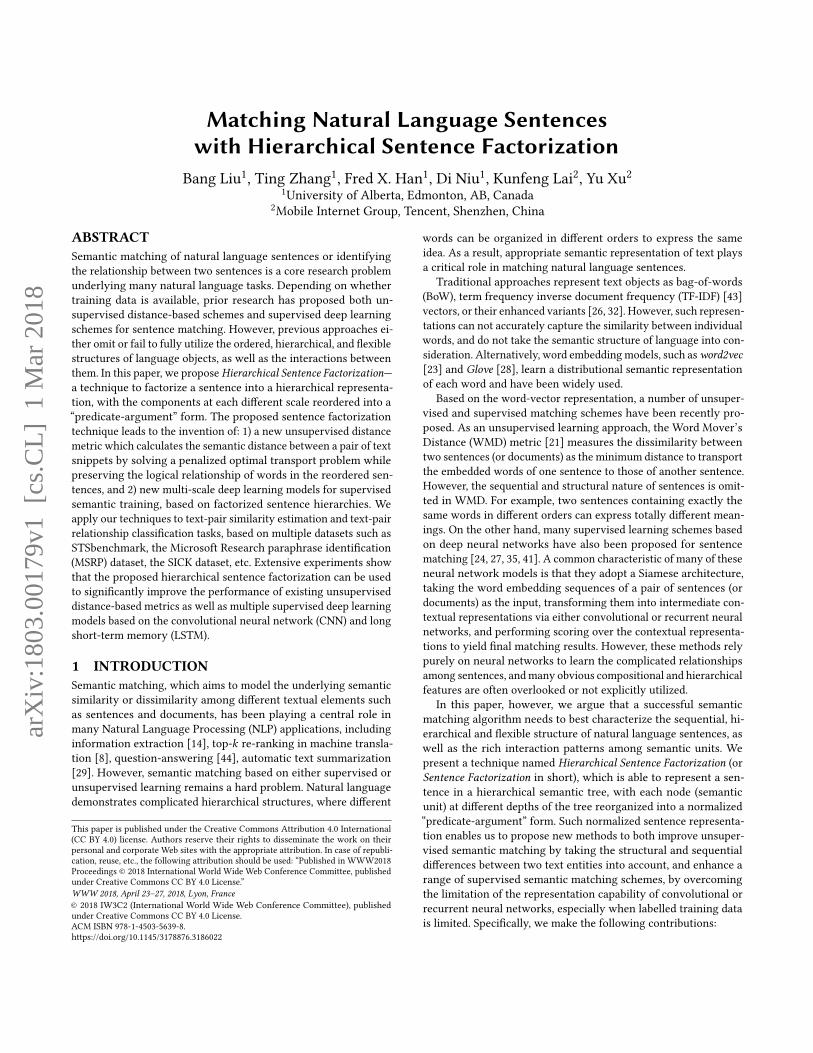
For example, in Fig. 1, we convert sentence A into a hierarchicalfactorization tree (a4) using a series of operations. The root nodeof the tree contains the semantic unit “chase Tom Jerry little yardbig”, which is the reordered representation of the original sentence“The little Jerry is being chased by Tom in the big yard” in a seman-tically normalized form. Moreover, the semantic unit at depth 0is factorized into four sub-units at depth 1: “chase”, “Tom”, “Jerrylittle” and “yard big”, each in the “predicate-argument” form. Andat depth 2, the semantic sub-unit “Jerry little” is further factorizedinto two sub-units “Jerry” and “little”. Finally, a semantic unit thatcontains only one token (e.g., “chase” and “Tom” at depth 1) cannot be further decomposed. Therefore, it only has one child nodeat the next depth through self-duplication.

We can observe that each depth of the tree contains all the tokens(except meaningless ones) in the original sentence, but re-organizesthese tokens into semantic units of different granularities.

2.1 Hierarchical Sentence FactorizationWe now describe our detailed procedure to transform a naturallanguage sentence to the desired factorization treementioned above.Our Hierarchical Sentence Factorization algorithm mainly consistsof five steps: 1) AMR parsing and alignment, 2) AMR purification,3) index mapping, 4) node completion, and 5) node traversal. Thelatter four steps are illustrated in the example in Fig. 1 from left toright.

AMR parsing and alignment. Given an input sentence, thefirst step of our hierarchical sentence factorization algorithm is

Sentence A: The little Jerry is being chased by Tom in the big yard.

Sentence B: The blue cat is catching the brown mouse in the forecourt.

chase !"#

Tom (0.0)

Jerry (0.1)

little (0.1.0)

yard (0.2)

big (0.2.0)

catch (0)

cat (0.0)

mouse (0.1)

brown (0.1.0)

forecourt (0.2)

blue (0.0.0)

( chase Tom ( Jerry little ) ( yard big ) )

( catch ( cat blue ) ( mouse brown ) forecourt )

chase

Tom

Jerry

little

yard

big

catc

h

cat

blu

e

mo

use

bro

wn

fore

co

urt

A. Original sentence pair to match

D. Semantic units alignment at different

semantic granularities

C. Normalized sentences that reordered

into predicate-argument form

chase (0.0)

Tom (0.1)

Jerry (0.2)

little (0.2.1)

yard (0.3)

big (0.3.1)

B. Steps to transform sentences into Sentence Factorization Trees

ROOT (0)

chase (0.0)

Tom (0.1)

Jerry (0.2)

little (0.2.1)

yard (0.3)

big (0.3.1)

ROOT (0)

chase (0.0.0)

Tom (0.1.0)

Jerry (0.2.0)

yard (0.3.0)

chase (0.0)

Tom (0.1)

Jerry little (0.2)

little (0.2.1)

yard big (0.3)

big (0.3.1)

chase Tom Jerry little yard big (0)

chase (0.0.0)

Tom (0.1.0)

Jerry (0.2.0)

yard (0.3.0)

ROOT (0)

cat (0.1)

mouse (0.2)

brown (0.2.1)

forecourt (0.3)

blue (0.1.1)

catch (0.0)

ROOT (0)

cat (0.1)

mouse (0.2)

brown (0.2.1)

forecourt (0.3)

blue (0.1.1)

catch (0.0)

catch (0.0.0)

cat (0.1.0)

mouse (0.2.0)

forecourt (0.3.0)

catch cat blue mouse brown forecourt (0)

cat blue(0.1)

mouse brown (0.2)

brown (0.2.1)

forecourt (0.3)

blue (0.1.1)

catch (0.0)

catch (0.0.0)

cat (0.1.0)

mouse (0.2.0)

forecourt (0.3.0)

AMR Purification Index Mapping Node Completion Node Travers!"

(a1) (a2) (a3) (a4)

(b1) (b2) (b3) (b4)

Figure 1: An example of the sentence factorization process. Here we show: A. The original sentence pair; B. The procedures ofcreating sentence factorization trees; C. The predicate-argument form of original sentence pair; D. The alignment of semanticunits with the reordered form.

(o / observe-01

:ARG0 (i / i)

:ARG1 (m / move-01

:ARG0 (a / army)

:manner (q / quick))

I observed that the army moved quickly.

0.0 0 0.1.0 0.1 0.1.1

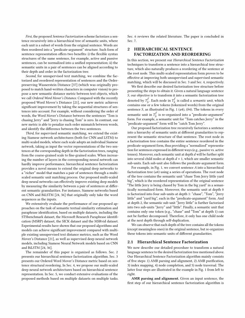
Figure 2: An example of a sentence and its AbstractMeaningRepresentation (AMR), as well as the alignment between thewords in the sentence and the nodes in AMR.

to acquire its Abstract Meaning Representation (AMR), as well asperform AMR-Sentence alignment to align the concepts in AMRwith the tokens in the original sentence.

Semantic parsing [2, 4, 6, 11, 18] can be performed to generatethe formal semantic representation of a sentence. Abstract Mean-ing Representation (AMR) [4] is a semantic parsing language thatrepresents a sentence by a directed acyclic graph (DAG). Each AMRgraph can be converted into an AMR tree by duplicating the nodesthat have more than one parent.

Fig. 2 shows the AMR of the sentence “I observed that the armymoved quickly.” In an AMR graph, leaves are labeled with con-cepts, which represent either English words (e.g., “army”), Prop-Bank framesets (e.g., “observe-01”) [18], or special keywords (e.g.,dates, quantities, world regions, etc.). For example, “(a / army)”refers to an instance of the concept army, where “a” is the variablename of army (each entity in AMR has a variable name). “ARG0”,“ARG1”, “:manner” are different kinds of relations defined in AMR.Relations are used to link entities. For example, “:manner” links “m/ move-01” and “q / quick”, which means “move in a quick manner”.Similarly, “:ARG0” links “m / move-01” and “a / army”, which meansthat “army” is the first argument of “move”.

Each leaf in AMR is a concept rather than the original token ina sentence. The alignment between a sentence and its AMR graphis not given in the AMR annotation. Therefore, AMR alignment[30] needs to be performed to link the leaf nodes in the AMR totokens in the original sentence. Fig. 2 shows the alignment betweensentence tokens and AMR concepts by the alignment indexes. Thealignment index 0 is for the root node, 0.0 for the first child of theroot node, 0.1 for the second child of the root node, and so forth. Forexample, in Fig. 2, the word “army” in sentence is linked with index“0.1.0”, which represents the concept node “a / army” in its AMR.

(d / dance-01

:ARG0 (k / kid

:mod (c / continent

:name (n / name

:op1 “Asia”)

:wiki “Asia”)

:quant 3))

Asian kids are dancing.

0.0.0+0.0.0.0+0.0.0.0.0+0.0.0.1

Three

dance

kid

Asia

3

Original AMR Purified Tree

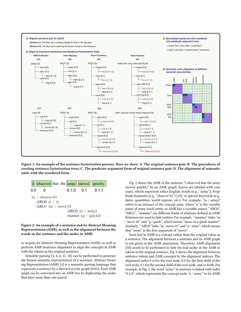
Figure 3: An example to show the operation of AMR purifi-cation.

We refer interested readers to [3, 4] for more detailed descriptionabout AMR.

Various parsers have been proposed for AMR parsing and align-ment [13, 39]. We choose the JAMR parser [13] in our algorithmimplementation.

AMR purification. Unfortunately, AMR itself cannot be usedto form the desired factorization tree. First, it is likely that multi-ple concepts in AMR may link to the same token in the sentence.For example, Fig. 3 shows AMR and its alignment for the sentence“Three Asian kids are dancing.”. The token “Asian” is linked to fourconcepts in the AMR graph: “ continent (0.0.0)”, “name (0.0.0.0)”,“Asia (0.0.0.0.0)” and “wiki Asia (0.0.0.1)”. This is because AMR willmatch a named entity with predefined concepts which it belongsto, such as “c / continent” for “Asia”, and form a compound repre-sentation of the entity. For example, in Fig.3, the token “Asian” isrepresented as a continent whose name is Asia, and its Wikipediaentity name is also Asia.

In this case, we select the link index with the smallest tree depthas the token’s position in the tree. Suppose Pw = {p1,p2, · · · ,p |P |}denotes the set of alignment indexes of token w . We can get thedesired alignment index ofw by calculating the longest commonprefix of all the index strings in Pw . After getting the alignmentindex for each token, we then replace the concepts in AMR with thetokens in sentence by the alignment indexes, and remove relationnames (such as “:ARG0”) in AMR, resulting into a compact treerepresentation of the original sentence, as shown in the right partof Fig. 3.

Index mapping. A purified AMR tree for a sentence obtainedin the previous step is still not in our desired form. To transform itinto a hierarchical sentence factorization tree, we perform indexmapping and calculate a new position (or index) for each token inthe desired factorization tree given its position (or index) in thepurified AMR tree. Fig. 1 illustrates the process of index mapping.After this step, for example, the purified AMR trees in Fig. 1 (a1)and (b1) will be transformed into (a2) and (b2).

Specifically, let TpS denote a purified AMR tree of sentence S ,and T

fS our desired sentence factorization tree of S . Let IpN =

i0.i1.i2. · · · .id denote the index of node N in TpS , where d is the

depth of N inTpS (where depth 0 represents the root of a tree). Then,the index I fN of node N in our desired factorization tree T f

S will be

Morty is laughing at Rick

Mortyis laughing atRick

Morty is laughing at Rick

WMD Matching

OWMD Matching

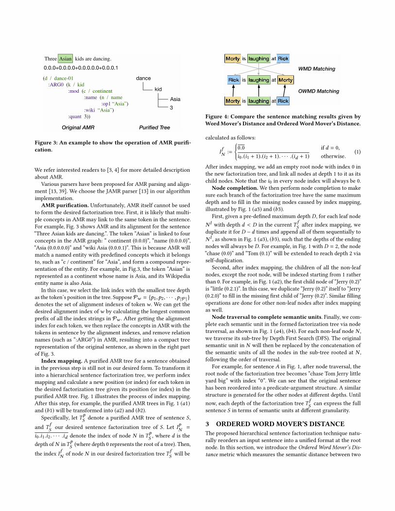
Figure 4: Compare the sentence matching results given byWordMover’s Distance andOrderedWordMover’s Distance.

calculated as follows:

IfN :=

{0.0 if d = 0,i0.(i1 + 1).(i2 + 1). · · · .(id + 1) otherwise.

(1)

After index mapping, we add an empty root node with index 0 inthe new factorization tree, and link all nodes at depth 1 to it as itschild nodes. Note that the i0 in every node index will always be 0.

Node completion. We then perform node completion to makesure each branch of the factorization tree have the same maximumdepth and to fill in the missing nodes caused by index mapping,illustrated by Fig. 1 (a3) and (b3).

First, given a pre-defined maximum depth D, for each leaf nodeN l with depth d < D in the current T f

S after index mapping, weduplicate it for D − d times and append all of them sequentially toN l , as shown in Fig. 1 (a3), (b3), such that the depths of the endingnodes will always be D. For example, in Fig. 1 with D = 2, the node“chase (0.0)” and “Tom (0.1)” will be extended to reach depth 2 viaself-duplication.

Second, after index mapping, the children of all the non-leafnodes, except the root node, will be indexed starting from 1 ratherthan 0. For example, in Fig. 1 (a2), the first child node of “Jerry (0.2)”is “little (0.2.1)”. In this case, we duplicate “Jerry (0.2)” itself to “Jerry(0.2.0)” to fill in the missing first child of “Jerry (0.2)”. Similar fillingoperations are done for other non-leaf nodes after index mappingas well.

Node traversal to complete semantic units. Finally, we com-plete each semantic unit in the formed factorization tree via nodetraversal, as shown in Fig. 1 (a4), (b4). For each non-leaf node N ,we traverse its sub-tree by Depth First Search (DFS). The originalsemantic unit in N will then be replaced by the concatenation ofthe semantic units of all the nodes in the sub-tree rooted at N ,following the order of traversal.

For example, for sentence A in Fig. 1, after node traversal, theroot node of the factorization tree becomes “chase Tom Jerry littleyard big” with index “0”. We can see that the original sentencehas been reordered into a predicate-argument structure. A similarstructure is generated for the other nodes at different depths. Untilnow, each depth of the factorization tree T f

S can express the fullsentence S in terms of semantic units at different granularity.

3 ORDEREDWORD MOVER’S DISTANCEThe proposed hierarchical sentence factorization technique natu-rally reorders an input sentence into a unified format at the rootnode. In this section, we introduce the Ordered Word Mover’s Dis-tance metric which measures the semantic distance between two

input sentences based on the unified representation of reorderedsentences.

Assume X ∈ Rd×n is a word2vec embedding matrix for a vo-cabulary of n words, and the i-th column xi ∈ Rd represents thed-dimensional embedding vector of i-th word in vocabulary. Denotea sentence S = a1a2 · · ·aK where ai represents the i-th word (orthe word embedding vector). The Word Mover’s Distance considersa sentence S as its normalized bag-of-words (nBOW) vectors wherethe weights of the words in S is α = {α1,α2, · · · ,αK }. Specifically,if word ai appears ci times in S , then αi =

ci∑Kj=1 c j

.The Word Mover’s Distance metric combines the normalized

bag-of-words representation of sentences with Wasserstein dis-tance (also known as Earth Mover’s Distance [33]) to measure thesemantic distance between two sentences. Given a pair of sentencesS1 = a1a2 · · ·aM and S2 = b1b2 · · ·bN , where bj ∈ Rd is the em-bedding vector of the j-th word in S2. Let α = {α1, · · · ,αM } andβ = {β1, · · · , βN } represents the normalized bag-of-words vectorsof S1 and S2. We can calculate a distance matrix D ∈ RM×N whereeach element Di j = ∥ai −bj ∥2 measures the distance between wordai and bj (we use the same notation to denote the word itself orits word vector representation). Let T ∈ RM×N be a non-negativesparse transport matrix where Ti j denotes the portion of wordai ∈ S1 that transports to word bj ∈ S2. The Word Mover’s Dis-tance between sentences S1 and S2 is given by

∑i, j Ti jDi j . The

transport matrix T is computed solving the following constrainedoptimization problem:

minimizeT ∈RM×N+

∑i, j

Ti jDi j

subject toM∑i=1

Ti j = βj 1 ≤ j ≤ N ,

N∑j=1

Ti j = αi 1 ≤ i ≤ M .

(2)

Where the minimum “word travel cost” between two bags of wordsfor a pair of sentences is calculated to measure the their semanticdistance.

However, the Word Mover’s Distance fails to consider a few as-pects of natural language. First, it omits the sequential structure. Forexample, in Fig. 4, the pair of sentences “Morty is laughing at Rick”and “Rick is laughing at Morty” only differ in the order of words.The Word Mover’s Distance metric will then find an exact matchbetween the two sentences and estimate the semantic distance aszero, which is obviously false. Second, the normalized bag-of-wordsrepresentation of a sentence can not distinguish duplicated wordsshown in multiple positions of a sentence.

To overcome the above challenges, we propose a new kind ofsemantic distance metric named Ordered Word Mover’s Distance(OWMD). The Ordered Word Mover’s Distance combines our sen-tence factorization technique with Order-preserving WassersteinDistance proposed in [37]. It casts the calculation of semantic dis-tance between texts as an optimal transport problem while preserv-ing the sequential structure of words in sentences. The OrderedWord Mover’s Distance differs from the Word Mover’s Distance inmultiple aspects.

First, rather than using normalized bag-of-words vector to rep-resent a sentence, we decompose and re-organize a sentence usingthe sentence factorization algorithm described in Sec. 2. Given asentence S , we represent it by the reordered word sequence S ′ inthe root node of its sentence factorization tree. Such representationnormalizes a sentence into “predicate-argument” structure to betterhandle syntactic variations. For example, after performing sentencefactorization, sentences “Tom is chasing Jerry” and “Jerry is beingchased by Tom” will both be normalized as “chase Tom Jerry”.

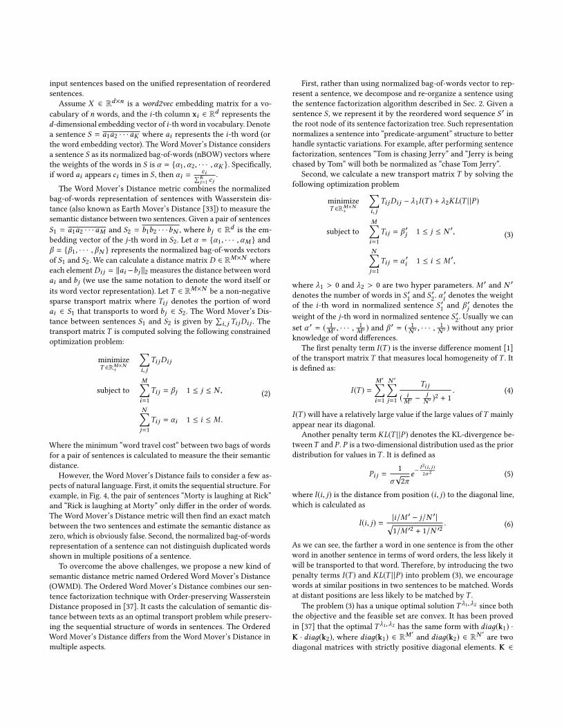
Second, we calculate a new transport matrix T by solving thefollowing optimization problem

minimizeT ∈RM×N+

∑i, j

Ti jDi j − λ1I (T ) + λ2KL(T | |P)

subject toM∑i=1

Ti j = β ′j 1 ≤ j ≤ N ′,

N∑j=1

Ti j = α ′i 1 ≤ i ≤ M ′,

(3)

where λ1 > 0 and λ2 > 0 are two hyper parameters. M ′ and N ′

denotes the number of words in S ′1 and S′2. α′i denotes the weight

of the i-th word in normalized sentence S ′1 and β ′j denotes theweight of the j-th word in normalized sentence S ′2. Usually we canset α ′ = ( 1

M ′ , · · · ,1M ′ ) and β ′ = ( 1

N ′ , · · · ,1N ′ ) without any prior

knowledge of word differences.The first penalty term I (T ) is the inverse difference moment [1]

of the transport matrix T that measures local homogeneity of T . Itis defined as:

I (T ) =M ′∑i=1

N ′∑j=1

Ti j

( iM ′ −

jN ′ )2 + 1

. (4)

I (T )will have a relatively large value if the large values ofT mainlyappear near its diagonal.

Another penalty term KL(T | |P) denotes the KL-divergence be-tweenT and P . P is a two-dimensional distribution used as the priordistribution for values in T . It is defined as

Pi j =1

σ√2π

e− l

2(i, j )2σ 2 (5)

where l(i, j) is the distance from position (i, j) to the diagonal line,which is calculated as

l(i, j) = |i/M ′ − j/N ′ |√1/M ′2 + 1/N ′2

. (6)

As we can see, the farther a word in one sentence is from the otherword in another sentence in terms of word orders, the less likely itwill be transported to that word. Therefore, by introducing the twopenalty terms I (T ) and KL(T | |P) into problem (3), we encouragewords at similar positions in two sentences to be matched. Wordsat distant positions are less likely to be matched by T .

The problem (3) has a unique optimal solution T λ1,λ2 since boththe objective and the feasible set are convex. It has been provedin [37] that the optimal T λ1,λ2 has the same form with diaд(k1) ·K · diaд(k2), where diaд(k1) ∈ RM

′ and diaд(k2) ∈ RN′ are two

diagonal matrices with strictly positive diagonal elements. K ∈

RM′×N ′ is a matrix defined as

Ki j = Pi je1λ2(Sλ1i j −Di j ), (7)

where

Si j =λ1

( iM ′ −

jN ′ )2 + 1

. (8)

The two matrices k1 and k2 can be efficiently obtained by theSinkhorn-Knopp iterative matrix scaling algorithm [19]:

k1 ← α ′./Kk2,

k2 ← β ′./KT k1.(9)

where ./ is the element-wise division operation. Compared withWord Mover’s Distance, the Ordered Word Mover’s Distance con-siders the positions of words in a sentence, and is able to distinguishduplicated words at different locations. For example, in Fig. 4, whilethe WMD finds an exact match and get a semantic distance of zerofor the sentence pair “Morty is laughing at Rick” and “Rick is laugh-ing at Morty”, the OWMD metric is able to find a better matchrelying on the penalty terms, and gives a semantic distance greaterthan zero.

The computational complexity of OWMD is also effectively re-duced compared to WMD. With the additional constraints, the timecomplexity is O(dM ′N ′) where d is the dimension of word vectors[37], while it isO(dp3 logp) for WMD, where p denotes the numberof uniques words in sentences or documents [21].

4 MULTI-SCALE SENTENCE MATCHINGOur sentence factorization algorithm parses a sentence S into ahierarchical factorization treeT f

S , where each depth ofT fS contains

the semantic units of the sentence at a different granularity. In thissection, we exploit this multi-scaled representation of S present inTfS to propose a multi-scaled Siamese network architecture thatcan extend any existing CNN or RNN-based Siamese architecturesto leverage the hierarchical representation of sentence semantics.

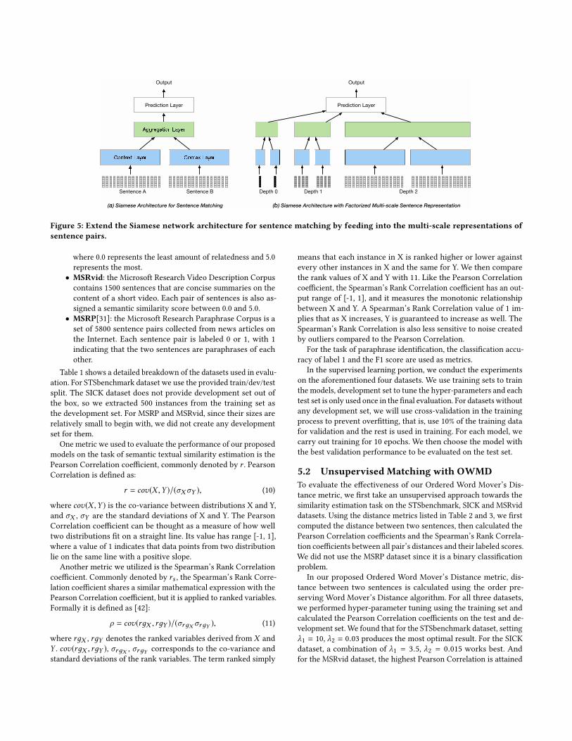
Fig. 5 (a) shows the network architecture of the popular Siamese“matching-aggregation” framework [5, 24, 25, 35, 40] for sentencematching tasks. The matching process is usually performed as fol-lows: First, the sequence of word embeddings in two sentenceswill be encoded by a context representation layer, which usuallycontains one or multiple layers of LSTM, bi-directional LSTM (BiL-STM), or CNN with max pooling layers. The goal is to capture thecontextual information of each sentence into a context vector. In aSiamese network, every sentence is encoded by the same contextrepresentation layer. Second, the context vectors of two sentenceswill be concatenated in the aggregation layer. They may be furthertransformed by more layers of neural network to get a fixed lengthmatching vector. Finally, a prediction layer will take in the matchingvector and outputs a similarity score for the two sentences or theprobability distribution over different sentence-pair relationships.

Compared with the typical Siamese network shown in Fig. 5 (a),our proposed architecture shown in Fig. 5 (b) differs in two aspects.First, our network contains three Siamese sub-modules that are sim-ilar to (a). They correspond to the factorized representations fromdepth 0 (the root layer) to depth 2. We only select the semantic unitsfrom the top 3 depths of the factorization tree as our input, because

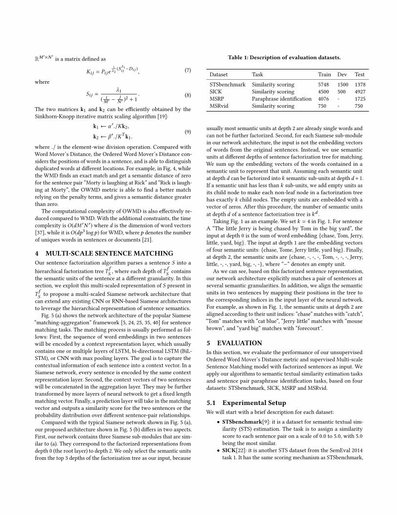
Table 1: Description of evaluation datasets.

Dataset Task Train Dev TestSTSbenchmark Similarity scoring 5748 1500 1378SICK Similarity scoring 4500 500 4927MSRP Paraphrase identification 4076 - 1725MSRvid Similarity scoring 750 - 750

usually most semantic units at depth 2 are already single words andcan not be further factorized. Second, for each Siamese sub-modulein our network architecture, the input is not the embedding vectorsof words from the original sentences. Instead, we use semanticunits at different depths of sentence factorization tree for matching.We sum up the embedding vectors of the words contained in asemantic unit to represent that unit. Assuming each semantic unitat depth d can be factorized into k semantic sub-units at depth d +1.If a semantic unit has less than k sub-units, we add empty units asits child node to make each non-leaf node in a factorization treehas exactly k child nodes. The empty units are embedded with avector of zeros. After this procedure, the number of semantic unitsat depth d of a sentence factorization tree is kd .

Taking Fig. 1 as an example. We set k = 4 in Fig. 1. For sentenceA “The little Jerry is being chased by Tom in the big yard”, theinput at depth 0 is the sum of word embedding {chase, Tom, Jerry,little, yard, big}. The input at depth 1 are the embedding vectorsof four semantic units: {chase, Tome, Jerry little, yard big}. Finally,at depth 2, the semantic units are {chase, -, -, -, Tom, -, -, -, Jerry,little, -, -, yard, big, -, -}, where “−” denotes an empty unit.

As we can see, based on this factorized sentence representation,our network architecture explicitly matches a pair of sentences atseveral semantic granularities. In addition, we align the semanticunits in two sentences by mapping their positions in the tree tothe corresponding indices in the input layer of the neural network.For example, as shown in Fig. 1, the semantic units at depth 2 arealigned according to their unit indices: “chase” matches with “catch”,“Tom” matches with “cat blue”, “Jerry little” matches with “mousebrown”, and “yard big” matches with “forecourt”.

5 EVALUATIONIn this section, we evaluate the performance of our unsupervisedOrdered Word Mover’s Distance metric and supervised Multi-scaleSentence Matching model with factorized sentences as input. Weapply our algorithms to semantic textual similarity estimation tasksand sentence pair paraphrase identification tasks, based on fourdatasets: STSbenchmark, SICK, MSRP and MSRvid.

5.1 Experimental SetupWe will start with a brief description for each dataset:• STSbenchmark[9]: it is a dataset for semantic textual sim-ilarity (STS) estimation. The task is to assign a similarityscore to each sentence pair on a scale of 0.0 to 5.0, with 5.0being the most similar.• SICK[22]: it is another STS dataset from the SemEval 2014task 1. It has the same scoring mechanism as STSbenchmark,

Sentence A Sentence B

Context Layer Contex Layer

Aggregation Layer

Prediction Layer Prediction Layer

(a) Siamese Architecture for Sentence Matching (b) Siamese Architecture with Factorized Multi-scale Sentence Representation

Depth 0 Depth 1 Depth 2

Output Output

Figure 5: Extend the Siamese network architecture for sentence matching by feeding into the multi-scale representations ofsentence pairs.

where 0.0 represents the least amount of relatedness and 5.0represents the most.• MSRvid: the Microsoft Research Video Description Corpuscontains 1500 sentences that are concise summaries on thecontent of a short video. Each pair of sentences is also as-signed a semantic similarity score between 0.0 and 5.0.• MSRP[31]: the Microsoft Research Paraphrase Corpus is aset of 5800 sentence pairs collected from news articles onthe Internet. Each sentence pair is labeled 0 or 1, with 1indicating that the two sentences are paraphrases of eachother.

Table 1 shows a detailed breakdown of the datasets used in evalu-ation. For STSbenchmark dataset we use the provided train/dev/testsplit. The SICK dataset does not provide development set out ofthe box, so we extracted 500 instances from the training set asthe development set. For MSRP and MSRvid, since their sizes arerelatively small to begin with, we did not create any developmentset for them.

One metric we used to evaluate the performance of our proposedmodels on the task of semantic textual similarity estimation is thePearson Correlation coefficient, commonly denoted by r . PearsonCorrelation is defined as:

r = cov(X ,Y )/(σXσY ), (10)

where cov(X ,Y ) is the co-variance between distributions X and Y,and σX , σY are the standard deviations of X and Y. The PearsonCorrelation coefficient can be thought as a measure of how welltwo distributions fit on a straight line. Its value has range [-1, 1],where a value of 1 indicates that data points from two distributionlie on the same line with a positive slope.

Another metric we utilized is the Spearman’s Rank Correlationcoefficient. Commonly denoted by rs , the Spearman’s Rank Corre-lation coefficient shares a similar mathematical expression with thePearson Correlation coefficient, but it is applied to ranked variables.Formally it is defined as [42]:

ρ = cov(rдX , rдY )/(σrдX σrдY ), (11)

where rдX , rдY denotes the ranked variables derived from X andY . cov(rдX , rдY ), σrдX , σrдY corresponds to the co-variance andstandard deviations of the rank variables. The term ranked simply

means that each instance in X is ranked higher or lower againstevery other instances in X and the same for Y. We then comparethe rank values of X and Y with 11. Like the Pearson Correlationcoefficient, the Spearman’s Rank Correlation coefficient has an out-put range of [-1, 1], and it measures the monotonic relationshipbetween X and Y. A Spearman’s Rank Correlation value of 1 im-plies that as X increases, Y is guaranteed to increase as well. TheSpearman’s Rank Correlation is also less sensitive to noise createdby outliers compared to the Pearson Correlation.

For the task of paraphrase identification, the classification accu-racy of label 1 and the F1 score are used as metrics.

In the supervised learning portion, we conduct the experimentson the aforementioned four datasets. We use training sets to trainthe models, development set to tune the hyper-parameters and eachtest set is only used once in the final evaluation. For datasets withoutany development set, we will use cross-validation in the trainingprocess to prevent overfitting, that is, use 10% of the training datafor validation and the rest is used in training. For each model, wecarry out training for 10 epochs. We then choose the model withthe best validation performance to be evaluated on the test set.

5.2 Unsupervised Matching with OWMDTo evaluate the effectiveness of our Ordered Word Mover’s Dis-tance metric, we first take an unsupervised approach towards thesimilarity estimation task on the STSbenchmark, SICK and MSRviddatasets. Using the distance metrics listed in Table 2 and 3, we firstcomputed the distance between two sentences, then calculated thePearson Correlation coefficients and the Spearman’s Rank Correla-tion coefficients between all pair’s distances and their labeled scores.We did not use the MSRP dataset since it is a binary classificationproblem.

In our proposed Ordered Word Mover’s Distance metric, dis-tance between two sentences is calculated using the order pre-serving Word Mover’s Distance algorithm. For all three datasets,we performed hyper-parameter tuning using the training set andcalculated the Pearson Correlation coefficients on the test and de-velopment set. We found that for the STSbenchmark dataset, settingλ1 = 10, λ2 = 0.03 produces the most optimal result. For the SICKdataset, a combination of λ1 = 3.5, λ2 = 0.015 works best. Andfor the MSRvid dataset, the highest Pearson Correlation is attained

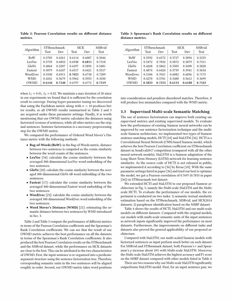
Table 2: Pearson Correlation results on different distancemetrics.

Algorithm STSbenchmark SICK MSRvidTest Dev Test Dev Test

BoW 0.5705 0.6561 0.6114 0.6087 0.5044LexVec 0.5759 0.6852 0.6948 0.6811 0.7318GloVe 0.4064 0.5207 0.6297 0.5892 0.5481Fastext 0.5079 0.6247 0.6517 0.6421 0.5517

Word2vec 0.5550 0.6911 0.7021 0.6730 0.7209WMD 0.4241 0.5679 0.5962 0.5953 0.3430OWMD 0.6144 0.7240 0.6797 0.6772 0.7519

when λ1 = 0.01, λ2 = 0.02. We maintain a max iteration of 20 sincein our experiments we found that it is sufficient for the correlationresult to converge. During hyper-parameter tuning we discoveredthat using the Euclidean metric along with σ = 10 produces bet-ter results, so all OWMD results summarized in Table 2 and 3are acquired under these parameter settings. Finally, it is worthmentioning that our OWMD metric calculates the distances usingfactorized versions of sentences, while all other metrics use the orig-inal sentences. Sentence factorization is a necessary preprocessingstep for the OWMD metric.

We compared the performance of Ordered Word Mover’s Dis-tance metric with the following methods:• Bag-of-Words (BoW): in the Bag-of-Words metric, distancebetween two sentences is computed as the cosine similaritybetween the word counts of the sentences.• LexVec [34]: calculate the cosine similarity between theaveraged 300-dimensional LexVec word embedding of thetwo sentences.• GloVe [28]: calculate the cosine similarity between the aver-aged 300-dimensional GloVe 6B word embedding of the twosentences.• Fastext [17]: calculate the cosine similarity between theaveraged 300-dimensional Fastext word embedding of thetwo sentences.• Word2vec [23]: calculate the cosine similarity between theaveraged 300-dimensional Word2vec word embedding of thetwo sentences.• Word Mover’s Distance (WMD) [21]: estimating the se-mantic distance between two sentences by WMD introducedin Sec. 3.

Table 2 and Table 3 compare the performance of different metricsin terms of the Pearson Correlation coefficients and the Spearman’sRank Correlation coefficients. We can see that the result of ourOWMD metric achieves the best performance on all the datasetsin terms of the Spearman’s Rank Correlation coefficients. It alsoproduced the best Pearson Correlation results on the STSbenchmarkand the MSRvid dataset, while the performance on SICK datasetsare close to the best. This can be attributed to the two characteristicsof OWMD. First, the input sentence is re-organized into a predicate-argument structure using the sentence factorization tree. Therefore,corresponding semantic units in the two sentences will be alignedroughly in order. Second, our OWMD metric takes word positions

Table 3: Spearman’s Rank Correlation results on differentdistance metrics.

Algorithm STSbenchmark SICK MSRvidTest Dev Test Dev Test

BoW 0.5592 0.6572 0.5727 0.5894 0.5233LexVec 0.5472 0.7032 0.5872 0.5879 0.7311GloVe 0.4268 0.5862 0.5505 0.5490 0.5828Fastext 0.4874 0.6424 0.5739 0.5941 0.5634

Word2vec 0.5184 0.7021 0.6082 0.6056 0.7175WMD 0.4270 0.5781 0.5488 0.5612 0.3699OWMD 0.5855 0.7253 0.6133 0.6188 0.7543

into consideration and penalizes disordered matches. Therefore, itwill produce less mismatches compared with the WMD metric.

5.3 Supervised Multi-scale Semantic MatchingThe use of sentence factorization can improve both existing un-supervised metrics and existing supervised models. To evaluatehow the performance of existing Siamese neural networks can beimproved by our sentence factorization technique and the multi-scale Siamese architecture, we implemented two types of Siamesesentence matching models, HCTI [24] and MaLSTM [36]. HCTI is aConvolutional Neural Network (CNN) based Siamese model, whichachieves the best Pearson Correlation coefficient on STSbenchmarkdataset in SemEval2017 competition (compared with all the otherneural network models). MaLSTM is a Siamese adaptation of theLong Short-Term Memory (LSTM) network for learning sentencesimilarity. As the source code of HCTI is not released in public,we implemented it according to [36] by Keras [10]. With the sameparameter settings listed in paper [36] and tried our best to optimizethe model, we got a Pearson correlation of 0.7697 (0.7833 in paper[36]) in STSbencmark test dataset.

We extended HCTI and MaLSTM to our proposed Siamese ar-chitecture in Fig. 5, namely the Multi-scale MaLSTM and the Multi-scale HCTI. To evaluate the performance of our models, the ex-periment is conducted on two tasks: 1) semantic textual similarityestimation based on the STSbenchmark, MSRvid, and SICK2014datasets; 2) paraphrase identification based on the MSRP dataset.

Table 4 shows the results of HCTI, MaLSTM and our multi-scalemodels on different datasets. Compared with the original models,our models with multi-scale semantic units of the input sentencesas network inputs significantly improved the performance on mostdatasets. Furthermore, the improvements on different tasks anddatasets also proved the general applicability of our proposed ar-chitecture.

Compared with MaLSTM, our multi-scaled Siamese models withfactorized sentences as input perform much better on each dataset.For MSRvid and STSbenmark dataset, both Pearson’s r and Spear-man’s ρ increase about 10% with Multi-scale MaLSTM. Moreover,the Multi-scale MaLSTM achieves the highest accuracy and F1 scoreon the MSRP dataset compared with other models listed in Table 4.

There are two reasonswhy ourMulti-scaleMaLSTM significantlyoutperforms MaLSTM model. First, for an input sentence pair, we

Table 4: A comparison among different supervised learning models in terms of accuracy, F1 score, Pearson’s r and Spearman’sρ on various test sets.

Model MSRP SICK MSRvid STSbenchmarkAcc.(%) F1(%) r ρ r ρ r ρ

MaLSTM 66.95 73.95 0.7824 0.71843 0.7325 0.7193 0.5739 0.5558Multi-scale MaLSTM 74.09 82.18 0.8168 0.74226 0.8236 0.8188 0.6839 0.6575

HCTI 73.80 80.85 0.8408 0.7698 0.8848 0.8763 0.7697 0.7549Multi-scale HCTI 74.03 81.76 0.8437 0.7729 0.8763 0.8686 0.7269 0.7033

explicitly model their semantic units with the factorization algo-rithm. Second, our multi-scaled network architecture is specificallydesigned for multi-scaled sentences representations. Therefore, it isable to explicitly match a pair of sentences at different granularities.

We also report the results of HCTI and Multi-scale HCTI inTable 4. For the paraphrase identification task, our model showsbetter accuracy and F1 score on MSRP dataset. For the semantictextual similarity estimation task, the performance varies acrossdatasets. On the SICK dataset, the performance of Multi-scale HCTIis close to HCTI with slightly better Pearson’ r and Spearman’s ρ.However, the Multi-scale HCTI is not able to outperform HCTI onMSRvid and STSbenchmark. HCTI is still the best neural networkmodel on the STSbenchmark dataset, and the MSRvid dataset is asubset of STSbenchmark. Although HCTI has strong performanceon these two datasets, it performs worse than our model on otherdatasets. Overall, the experimental results demonstrated the generalapplicability of our proposed model architecture, which performswell on various semantic matching tasks.

6 RELATEDWORKThe task of natural language sentence matching has been exten-sively studied for a long time. Here we review related unsupervisedand supervised models for sentence matching.

Traditional unsupervised metrics for document representation,including bag of words (BOW), term frequency inverse documentfrequency (TF-IDF) [43], Okapi BM25 score [32]. However, theserepresentations can not capture the semantic distance betweenindividual words. Topic modeling approaches such as Latent Se-mantic Indexing (LSI) [12] and Latent Dirichlet Allocation (LDA) [7]attempt to circumvent the problem through learning a latent rep-resentation of documents. But when applied to semantic-distancebased tasks such as text-pair semantic similarity estimation, thesealgorithms usually cannot achieve good performance.

Learning distributional representation for words, sentences ordocuments based on deep learning models have been popular re-cently. word2vec [23] and Glove [28] are two high quality wordembeddings that have been extensively used in many NLP tasks.Based on word vector representation, the Word Mover’s Distance(WMD) [21] algorithm measures the dissimilarity between two sen-tences (or documents) as the minimum distance that the embeddedwords of one sentence need to “travel” to reach the embedded wordsof another sentence. However, when applying these approaches tosentence pair matching tasks, the interactions between sentencepairs are omitted, also the ordered and hierarchical structure ofnatural languages is not considered.

Different neural network architectures have been proposed forsentence pair matching tasks. Models based on Siamese architec-tures [5, 24, 25, 35] usually transform the word embedding se-quences of text pairs into context representation vectors througha multi-layer Long Short-Term Memory (LSTM) [38] network orConvolutional Neural Networks (CNN) [20], followed by a fullyconnected network or score function which gives the similarityscore or classification label based on the context representationvectors. However, Siamese models defer the interaction betweentwo sentences until the hidden representation layer, therefore maylose details of sentence pairs for matching tasks [16].

Aside from Siamese architectures, [41] introduced a matchinglayer into Siamese network to compare the contextual embedding ofone sentence with another. [16, 27] proposed convolutional match-ing models that consider all pair-wise interactions between wordsin sentence pairs. [15] propose to explicitly model pairwise wordinteractions with a pairwise word interaction similarity cube and asimilarity focus layer to identify important word interactions.

7 CONCLUSIONIn this paper, we propose a technique named Hierarchical SentenceFactorization that is able to transform a sentence into a hierarchicalfactorization tree. Each node in the tree is a semantic unit consistsof one or several words in the sentence and reorganized into theform of “predicate-argument” structure. Each depth in the tree fac-torizes the sentence into semantic units of different scales. Basedon the hierarchical tree-structured representation of sentences, wepropose both an unsupervised metric and two supervised deepmodels for sentence matching tasks. On one hand, we design a newunsupervised distance metric, named Ordered Word Mover’s Dis-tance (OWMD), to measure the semantic difference between a pairof text snippets. OWMD takes the sequential structure of sentencesinto account, and is able to handle the flexible syntactical structureof natural language sentences. On the other hand, we propose themulti-scale Siamese neural network architecture which takes themulti-scale representation of a pair of sentences as network inputand matches the two sentences at different granularities.

We apply our techniques to the task of text-pair similarity esti-mation and the task of text-pair paraphrase identification, basedon multiple datasets. Our extensive experiments show that boththe unsupervised distance metric and the supervised multi-scaleSiamese network architecture can achieve significant improvementon multiple datasets using the technique of sentence factorization.

REFERENCES[1] Fritz Albregtsen et al. 2008. Statistical texture measures computed from gray level

coocurrence matrices. Image processing laboratory, department of informatics,university of oslo 5 (2008).

[2] Collin F Baker, Charles J Fillmore, and John B Lowe. 1998. The berkeley framenetproject. In Proceedings of the 36th Annual Meeting of the Association for Computa-tional Linguistics and 17th International Conference on Computational Linguistics-Volume 1. Association for Computational Linguistics, 86–90.

[3] Laura Banarescu, Claire Bonial, Shu Cai, Madalina Georgescu, Kira Griffitt, UlfHermjakob, Kevin Knight, Philipp Koehn, Martha Palmer, and Nathan Schneider.2012. Abstract meaning representation (AMR) 1.0 specification. In Parsing onFreebase from Question-Answer Pairs. In Proceedings of the 2013 Conference onEmpirical Methods in Natural Language Processing. Seattle: ACL. 1533–1544.

[4] Laura Banarescu, Claire Bonial, Shu Cai, Madalina Georgescu, Kira Griffitt, UlfHermjakob, Kevin Knight, Philipp Koehn, Martha Palmer, and Nathan Schneider.2013. Abstract meaning representation for sembanking. In Proceedings of the 7thLinguistic Annotation Workshop and Interoperability with Discourse. 178–186.

[5] Petr Baudiš, Jan Pichl, Tomáš Vyskočil, and Jan Šedivy. 2016. Sentence pairscoring: Towards unified framework for text comprehension. arXiv preprintarXiv:1603.06127 (2016).

[6] Jonathan Berant and Percy Liang. 2014. Semantic Parsing via Paraphrasing.. InACL (1). 1415–1425.

[7] DavidMBlei, Andrew YNg, andMichael I Jordan. 2003. Latent dirichlet allocation.Journal of machine Learning research 3, Jan (2003), 993–1022.

[8] Peter F Brown, Vincent J Della Pietra, Stephen A Della Pietra, and Robert LMercer. 1993. The mathematics of statistical machine translation: Parameterestimation. Computational linguistics 19, 2 (1993), 263–311.

[9] Daniel Cer, Mona Diab, Eneko Agirre, Inigo Lopez-Gazpio, and Lucia Specia. 2017.SemEval-2017 Task 1: Semantic Textual Similarity-Multilingual and Cross-lingualFocused Evaluation. arXiv preprint arXiv:1708.00055 (2017).

[10] François Chollet et al. 2015. Keras. https://github.com/fchollet/keras. (2015).[11] Marco Damonte, Shay B Cohen, and Giorgio Satta. 2016. An incremental parser

for abstract meaning representation. arXiv preprint arXiv:1608.06111 (2016).[12] Scott Deerwester, Susan T Dumais, George W Furnas, Thomas K Landauer, and

Richard Harshman. 1990. Indexing by latent semantic analysis. Journal of theAmerican society for information science 41, 6 (1990), 391.

[13] Jeffrey Flanigan, Sam Thomson, Jaime G Carbonell, Chris Dyer, and Noah ASmith. 2014. A discriminative graph-based parser for the abstract meaningrepresentation. (2014).

[14] Ralph Grishman. 1997. Information extraction: Techniques and challenges. InInformation extraction a multidisciplinary approach to an emerging informationtechnology. Springer, 10–27.

[15] Hua He and Jimmy J Lin. 2016. Pairwise Word Interaction Modeling with DeepNeural Networks for Semantic Similarity Measurement.. In HLT-NAACL. 937–948.

[16] Baotian Hu, Zhengdong Lu, Hang Li, and Qingcai Chen. 2014. Convolutional neu-ral network architectures for matching natural language sentences. In Advancesin neural information processing systems. 2042–2050.

[17] Armand Joulin, Edouard Grave, Piotr Bojanowski, and Tomas Mikolov. 2016. Bagof tricks for efficient text classification. arXiv preprint arXiv:1607.01759 (2016).

[18] Paul Kingsbury and Martha Palmer. 2002. From TreeBank to PropBank.. In LREC.1989–1993.

[19] Philip A Knight. 2008. The Sinkhorn–Knopp algorithm: convergence and appli-cations. SIAM J. Matrix Anal. Appl. 30, 1 (2008), 261–275.

[20] Alex Krizhevsky, Ilya Sutskever, and Geoffrey E Hinton. 2012. Imagenet classifica-tion with deep convolutional neural networks. In Advances in neural informationprocessing systems. 1097–1105.

[21] Matt Kusner, Yu Sun, Nicholas Kolkin, and Kilian Weinberger. 2015. From wordembeddings to document distances. In International Conference on Machine Learn-ing. 957–966.

[22] MarcoMarelli, StefanoMenini, Marco Baroni, Luisa Bentivogli, Raffaella Bernardi,and Roberto Zamparelli. 2014. A SICK cure for the evaluation of compositionaldistributional semantic models.. In LREC. 216–223.

[23] Tomas Mikolov, Kai Chen, Greg Corrado, and Jeffrey Dean. 2013. Efficientestimation of word representations in vector space. arXiv preprint arXiv:1301.3781(2013).

[24] Jonas Mueller and Aditya Thyagarajan. 2016. Siamese Recurrent Architecturesfor Learning Sentence Similarity.. In AAAI. 2786–2792.

[25] Paul Neculoiu, Maarten Versteegh, Mihai Rotaru, and Textkernel BV Amsterdam.2016. Learning Text Similarity with Siamese Recurrent Networks. ACL 2016(2016), 148.

[26] Georgios Paltoglou and Mike Thelwall. 2010. A study of information retrievalweighting schemes for sentiment analysis. In Proceedings of the 48th annual meet-ing of the association for computational linguistics. Association for ComputationalLinguistics, 1386–1395.

[27] Liang Pang, Yanyan Lan, Jiafeng Guo, Jun Xu, Shengxian Wan, and Xueqi Cheng.2016. Text Matching as Image Recognition.. In AAAI. 2793–2799.

[28] Jeffrey Pennington, Richard Socher, and Christopher Manning. 2014. Glove:Global vectors for word representation. In Proceedings of the 2014 conference onempirical methods in natural language processing (EMNLP). 1532–1543.

[29] Luca Ponzanelli, Andrea Mocci, and Michele Lanza. 2015. Summarizing complexdevelopment artifacts by mining heterogeneous data. In Proceedings of the 12thWorking Conference on Mining Software Repositories. IEEE Press, 401–405.

[30] Nima Pourdamghani, Yang Gao, Ulf Hermjakob, and Kevin Knight. 2014. AligningEnglish Strings with Abstract Meaning Representation Graphs.. In EMNLP. 425–429.

[31] Chris Quirk, Chris Brockett, and William Dolan. 2004. Monolingual machinetranslation for paraphrase generation. In Proceedings of the 2004 conference onempirical methods in natural language processing.

[32] Stephen E Robertson and Steve Walker. 1994. Some simple effective approxima-tions to the 2-poisson model for probabilistic weighted retrieval. In Proceedings ofthe 17th annual international ACM SIGIR conference on Research and developmentin information retrieval. Springer-Verlag New York, Inc., 232–241.

[33] Yossi Rubner, Carlo Tomasi, and Leonidas J Guibas. 2000. The earth mover’sdistance as a metric for image retrieval. International journal of computer vision40, 2 (2000), 99–121.

[34] Alexandre Salle, Marco Idiart, and Aline Villavicencio. 2016. Enhancing theLexVec Distributed Word Representation Model Using Positional Contexts andExternal Memory. arXiv preprint arXiv:1606.01283 (2016).

[35] Aliaksei Severyn andAlessandroMoschitti. 2015. Learning to rank short text pairswith convolutional deep neural networks. In Proceedings of the 38th InternationalACM SIGIR Conference on Research and Development in Information Retrieval.ACM, 373–382.

[36] Yang Shao. 2017. HCTI at SemEval-2017 Task 1: Use convolutional neural networkto evaluate semantic textual similarity. In Proceedings of the 11th InternationalWorkshop on Semantic Evaluation (SemEval-2017). 130–133.

[37] Bing Su and Gang Hua. 2017. Order-preserving wasserstein distance for sequencematching. In Proc. IEEE Conf. Comput. Vis. Pattern Recognit. 1049–1057.

[38] Martin Sundermeyer, Ralf Schlüter, and Hermann Ney. 2012. LSTM neural net-works for language modeling. In Thirteenth Annual Conference of the InternationalSpeech Communication Association.

[39] Chuan Wang, Nianwen Xue, and Sameer Pradhan. 2015. Boosting Transition-based AMR Parsing with Refined Actions and Auxiliary Analyzers.. In ACL (2).857–862.

[40] Shuohang Wang and Jing Jiang. 2016. A Compare-Aggregate Model for MatchingText Sequences. arXiv preprint arXiv:1611.01747 (2016).

[41] Zhiguo Wang, Wael Hamza, and Radu Florian. 2017. Bilateral multi-perspectivematching for natural language sentences. arXiv preprint arXiv:1702.03814 (2017).

[42] Wikipedia. 2017. Spearman’s rank correlation coefficient — Wikipedia,The Free Encyclopedia. (2017). https://en.wikipedia.org/w/index.php?title=Spearman%27s_rank_correlation_coefficient&oldid=801404677 [Online; accessed31-October-2017].

[43] Ho Chung Wu, Robert Wing Pong Luk, Kam Fai Wong, and Kui Lam Kwok. 2008.Interpreting tf-idf term weights as making relevance decisions. ACM Transactionson Information Systems (TOIS) 26, 3 (2008), 13.

[44] Lei Yu, Karl Moritz Hermann, Phil Blunsom, and Stephen Pulman. 2014. Deeplearning for answer sentence selection. arXiv preprint arXiv:1412.1632 (2014).