Embed Size (px)
Citation preview

Math 130 J.Jeneralczuk Final Exam Spring 2013
\
NAME:
.
You must show all work, calculations, formulas used to receive any credit.
NO WORK =NO CREDIT.
Round the final answers to 3 decimal places.
Good luck!
Question 1
Question 2
Question 3
Question 4
Question 5
Question 6
Question 7
Question 8
Total out of 100.

1. General Question. Several scenarios are listed below on the left. A number of statistical procedures, distribution,
and measures that we’ve covered are listed on the right. For each scenario, list the statistical method you should use.
Not all of the procedures listed will be used.
You wish test a hypothesis about a mean
using a small sample size. What procedure
should you use?
_______
You’d like to look for outliers in your data.
The distribution is skewed, though, so you’ve
opted to use the five number summary. What
procedure will help you identify possible
outliers?
_______
Which measure can be used to find the
relative standing of two observations from
different distributions of data?
_______
You are taking a sample of 50 people and
measuring their average height. Suppose the
individual heights have a mean of 56 inches
and a standard deviation of 5 inches. What
distribution would help you find the
probability that the average is greater than 70
inches tall?
_______
A health professional selected a random
sample of 100 patients from each of four
major hospital emergency rooms to see if the
major reasons for emergency room visits are
similar in all four major hospitals. The major
reason categories are accident, illegal activity,
illness, and other.
_______
A study wanted to examine the relationship
between number of Japanese beetle grubs and
percentage of organic matter in the soil for
locations on a golf course in New York..
_______
Bar Graph
Pie Chart
Mean and Standard deviation
Five Number Summary
1.5 IQR rule
Z-score
Histogram
Stem-and-leaf Plot
Boxplot
Binomial Distribution
Normal Distribution
Uniform Distribution
One-sample t-Interval for a mean
Two-sample t-Interval for a mean
One-sample z-Interval for a
proportion
Two-sample z-Interval for a
proportion
Matched pairs t-Test
One-sample t-Test for a mean
Two-sample t-Test for a mean
One-sample z-Test for a
proportion
Two-sample z-Test for a
proportion
ANOVA
Linear regression
Chi-squared goodness of fit
Chi-squared test for homogeneity
Chi-squared test for independence

A study compared the toxicity on flies of four
different types of selenium. The number of
dead flies was counted and the selenium type
(type 1, 2, 3, or 4) was recorded for each
observation. The researchers want to know if
the toxicities differ between selenium types
_______
You have a quantitative variable, and want to
visually picture the data in such a way that the
original data values are preserved. What
graph will do this?
_______
You’d like to find the mean income of all
Amherst residents, using a sample of 35
people. What procedure should you used to
produce a 95% confidence interval?
_______
You’d like to see if there is a difference in the
mean incoming SAT score of incoming
freshmen among all of the five colleges
_______

2. A biologist studying lizards, specifically
Cophosaurus texanus, recorded the weight
(mass) in grams, snout-vent length (SVL) and
hind limb span (HLS) of a random sample of 25
such lizards. The biologist wants to study the
relationship between variables, looking to see if
SVL can be used to predict weight (mass)
accurately. A basic scatterplot shows the data at
right.
a. Based on the scatterplot, how would you
describe the relationship between SVL and
mass?
A student working in the biologist’s lab runs a regression analysis on the data and produces the following partial Rcmdr
output:
Coefficients:
Estimate Std. Error t value Pr(>|t|)
(Intercept) -13.51551 1.22931 -10.99 1.24e-10 ***
SVL 0.32459 0.01786 18.18 3.84e-15 ***
---
Signif. codes: 0 '***' 0.001 '**' 0.01 '*' 0.05 '.' 0.1 ' ' 1
Residual standard error: 0.6986 on 23 degrees of freedom
Multiple R-squared: 0.9349, Adjusted R-squared: 0.9321
F-statistic: 330.5 on 1 and 23 DF, p-value: 3.836e-15
b. What is the value of the sample correlation coefficient? Interpret the correlation coefficient.
c. Interpret the R-squared value. How well you think this model fits the data?

d. What is the equation of the least squares regression line
e Check the assumptions .
f. Now , we want to assess whether or not SVL can be used to predict mass (weight) .What hypotheses correspond to
determining if SVL is a significant predictor
Null hypothesis: Alternative Hypothesis :
Test Statistic:
Distribution of Test Stat:
p-value :
Conclusion:
g. Obtain a 95% confidence interval for the population slope. (You do not need to list assumptions.) .

Interpret your interval
Can you conclude the population slope is less than 1? Explain.
h. Obtain predictions for mass based on SVLs of 64 and 98, if appropriate. If inappropriate, explain why.
i. Compute a 95% prediction interval for an individual response when SLVs=64. Interpret your interval .Assume the mean
value of SLV is 70 .
j. Compute a 95% confidence Interval for the mean response when SLVs=64. Interpret your interval

k. Which of the following aspects of the scatterplot affect the standard error of the regression slope?
A. spread around the line: se
B. spread of the x values: sx
C. sample size: n
D. all of the above
3. Researchers in 3 different cities decided to compare average pH of rainwater from their cities based on data collected
over the past 6 months. Each researcher obtained a random sample of pHs for their city. Help the researchers determine
whether their cities have the same or different average pH levels for rain. Preliminary analysis and formal analysis output
is given below from Rcmdr. Note: pH = 7 is neutral. Values below 7 are acidic, and normal rainwater has a pH of 5.3,
while acid rain is even lower.
Preliminary analysis:
mean sd 0% 25% 50% 75% 100% n
city1 5.164 0.1950910 4.68 5.0600 5.14 5.2800 5.75 40
city2 4.980 0.1369260 4.71 4.8875 4.95 5.0550 5.29 40
city3 5.100 0.1026570 4.90 5.0300 5.09 5.1625 5.32 40
a)What does the preliminary analysis reveal to you?

b. What assumptions need to be met? Do they appear to check out?
c. (Circle one) This ANOVA is balanced unbalanced
d. Determine the missing values for the degrees of freedom and the test statistic. . Use the output to complete the test you
set up hypotheses for, assuming all conditions check out.
Type df= F value=
Residuals df=
Df Sum Sq Mean Sq F value Pr(>F)
City ? 0.69803 0.34901 ? 1.029e-06 ***
Residuals ? 2.62656 0.02245
Null hypothesis: Alternative Hypothesis :
Test Statistic:
Distribution of Test Stat:
p-value :

Conclusion:
e. What is your best estimate of the common population variance?
f. Are multiple comparisons appropriate? Explain. If yes, summarize the results.
Multiple Comparisons of Means: Tukey Contrasts
95% family-wise confidence level
Linear Hypotheses:
Estimate lwr upr
city2 - city1 == 0 -0.18400 -0.26353 -0.10447
city3 - city1 == 0 -0.06400 -0.14353 0.01553
city3 - city2 == 0 0.12000 0.04047 0.19953
Multiple Comparisons (if appropriate):
Compute a 95% confidence interval for City1 – City 2 (by hand)
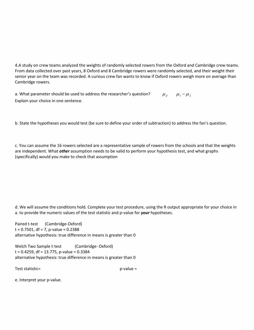
4.A study on crew teams analyzed the weights of randomly selected rowers from the Oxford and Cambridge crew teams. From data collected over past years, 8 Oxford and 8 Cambridge rowers were randomly selected, and their weight their senior year on the team was recorded. A curious crew fan wants to know if Oxford rowers weigh more on average than Cambridge rowers.
a. What parameter should be used to address the researcher’s question? d 21
Explain your choice in one sentence. b. State the hypotheses you would test (be sure to define your order of subtraction) to address the fan’s question. c. You can assume the 16 rowers selected are a representative sample of rowers from the schools and that the weights are independent. What other assumption needs to be valid to perform your hypothesis test, and what graphs (specifically) would you make to check that assumption d. We will assume the conditions hold. Complete your test procedure, using the R output appropriate for your choice in a. to provide the numeric values of the test statistic and p-value for your hypotheses. Paired t-test (Cambridge-Oxford) t = 0.7501, df = 7, p-value = 0.2388 alternative hypothesis: true difference in means is greater than 0 Welch Two Sample t-test (Cambridge- Oxford) t = 0.4259, df = 13.775, p-value = 0.3384 alternative hypothesis: true difference in means is greater than 0 Test statistic= p-value = e. Interpret your p-value.

f. Circle your decision at a .10 significance level. State your conclusion g. What type of error might you have made? Type I Type II No Error
5.Three students from Math 130, would like to investigate the habits of Amherst population in terms of athletic status and
environmentally conscious habits.in particular, whether or not they compost at Val.
a. What is the appropriate analysis to perform (be specific) and state appropriate hypotheses.
Analysis:
Null:
Alternative:
b. The two-way table below summaries the result from the survey. Observed (Expected) is the table setup.
Athletic Status \
Compost
YES NO Total
Varsity Athlete 41 ( 43.73 ) 8 ( 5.27 ) 49
Non-Varsity
Athlete
28 ( ) 3 ( ) 31
Non-Athlete 72 ( ) 6 ( 8.39 ) 78
Total 141 17 158
Please fill in expected counts in the table

c List and check the conditions for your test procedure..
d Compute your df, and find the test statistic and p-value.
Test statistic:
df=
p-value=
f. Decision at a α=0.05 significance level
6. Another four students from Math 130 are also interested in students‟ composting habit, but they are more curious about
its association with gender and run an appropriate test for their analysis. The two-way table below summaries the
corresponding result. Observed (Expected) is the table setup.
Gender \ Compost YES NO
Male 48 ( 54.39 ) 13 ( 6.61
Female 92 ( 85.61 ) 4 ( 10.39 )
Assume the assumptions for the test are all met. The test statistic works out to be 11.355. State your complete conclusion
in context.
Analysis:
Null:
Alternative:
df=
p-value=

Decision at a α=0.05 significance level
7. The overpopulation of Canadian Geese and their refusal to migrate because they are able to find food during the winter
has caused some environmental problems. In particular, their feces run off into rivers and lakes when it rains and fertilizes
algae (the reason why the campus pond is green).The abundance of algae blocks out the sun and makes it hard for other
aquatic plants to undergo photosynthesis. If the proportion of algae in the water exceeds 70%, then the aquatic plants will
not get enough sun and die, reducing the oxygen in the water which would then kill fish. A researcher, who is interested in
extending the hunting season for the geese, is going to test to see if the campus pond has enough algae to start killing fish.
In a sample of 100 pounds of water he finds that there is 85 pounds of algae. The researcher is interested in α = 0.05 level
test.
State the null and alternative hypotheses.
Select the distribution to use (check first) and write down the appropriate test statistic.
Compute the p-value of the test statistic
State your conclusion (in one sentence, state whether or not the test rejects the null hypothesis and in another sentence
apply the results to the problem).

Describe the Type I error (in one or two sentences).What are the consequences of making a Type I error?
Describe the Type II error (in one or two sentences).What are the consequences of making a Type II error?
8. Suppose the average mileage rating (in miles per gallon) of a particular model car is 28 mpg with a standard deviation
of 8 mpg. A random sample of 64 cars of this model is selected.
a) Completely describe the sampling distribution of the sample mean.
b) What is the probability that the sample mean exceeds 32mpg? Do you have to make any assumptions? Explain why or
why not

c) If one car is selected at random, what is the probability that the mileage rating exceeds 32mpg? Do you have to make
any assumptions? Explain why or why not.
d) If a randomly selected car has a mileage rating (in miles per gallon) of 55mpg, would you consider this unusual? Justify your
answer with calculations.
What conclusion might you draw?
e) If your random sample actually produced a sample mean equal to 55mpg, would you consider this unusual? Justify
your answer with calculations
What conclusion might you draw?