Embed Size (px)
Citation preview

MATH 350: Introduction to ComputationalMathematics
Chapter II: Solving Systems of Linear Equations
Greg Fasshauer
Department of Applied MathematicsIllinois Institute of Technology
Spring 2011
[email protected] MATH 350 – Chapter 2 1

Outline1 Applications, Motivation and Background Information
2 Gaussian Elimination = LU Decomposition
3 Forward and Back Substitution in MATLAB
4 Partial Pivoting
5 MATLAB Implementation of LU-Decomposition
6 Roundoff Error and the Condition Number of a Matrix
7 Special Matrices
8 An Application: Google’s Page Rank
[email protected] MATH 350 – Chapter 2 2

Applications, Motivation and Background Information Applications
Where do systems of linear equations come up?Everywhere!
They appear straightforwardly inanalytic geometry (intersection of lines and planes),traffic flow networks,Google page ranks,linear optimization problems (MATH 435),Leontief’s input-output model in economics,electric circuit problems,the steady-state analysis of a system of chemical or biologicalreactors,the structural analysis of trusses,and many other applications.
They will appear as intermediate or final steps in many numericalmethods such as
polynomial or spline interpolation (Ch. 3),the solution of nonlinear systems (Ch. 4),least squares fitting,the solution of systems of differential equations (Ch. 6),and many other advanced numerical methods.
[email protected] MATH 350 – Chapter 2 4

Applications, Motivation and Background Information Representation of Linear Systems
Equation form:
x1 + 2x2 + 3x3 = 12x1 + x2 + 4x3 = 13x1 + 4x2 + x3 = 1
Matrix form: Ax = b, with
A =
1 2 32 1 43 4 1
, x =
x1x2x3
, b =
111
.Note: We will always think of vectors as column vectors. If we need torefer to a row vector we will use the notation xT .
RemarkMost of the material discussed in this chapter can be found in Chapter2 of [NCM].
[email protected] MATH 350 – Chapter 2 5

Applications, Motivation and Background Information Avoid Inverses
Never use A−1 to solve Ax = b
In linear algebra we learn that the solution of
Ax = b
is given byx = A−1b.
This is correct, but inefficient and more prone to roundoff errors.
Always solve linear systems (preferably with some decompositionmethod such as LU, QR or SVD).
[email protected] MATH 350 – Chapter 2 6

Applications, Motivation and Background Information Avoid Inverses
Never use A−1 to solve Ax = b (cont.)ExampleConsider the trivial “system” 7x = 21 and compare solution via the“inverse” and by straightforward division.
Solution
Division immediately yields x = 217 = 3.
Use of the “inverse” yields
x = 7−1 × 21 = 0.142857× 21 = 2.999997.
Clearly, use of the inverse requires more work (first compute theinverse, then multiply it into the right-hand side), and it is less accurate.This holds even more so for larger systems of equations.
Note that MATLAB is “smarter” than this so that 7^(-1)*21 is stillequal 3 (but slower than division, see division.m).
[email protected] MATH 350 – Chapter 2 7

Applications, Motivation and Background Information Matrix Division in MATLAB
How to solve linear systems by “division” in MATLAB
In order to mimic what we do (naturally) for a single equation, MATLAB
provides two very sophisticated matrix division operators:For systems AX = B, we have the backslash (or mldivide)operator, i.e.,
X = A\B,
and XA = B is solved using a forward slash or (mrdivide)operator, i.e.,
X = B/A.
RemarkThese operators provide black boxes for the solution of (possibly evennon-square or singular) systems of linear equations.
We now want to understand a bit of what goes on “inside” thealgorithms.
[email protected] MATH 350 – Chapter 2 8

Applications, Motivation and Background Information A Simple Example
ExampleSolve the 3× 3 linear system
x1 + 2x2 + 3x3 = 12x1 + x2 + 4x3 = 13x1 + 4x2 + x3 = 1
using a simple (easily programmable) algorithm.
SolutionThe main idea is to systematically reduce the system to uppertriangular form since triangular systems are easy to solve.Thus, we will have
an elimination phase (resulting in an upper triangular system),and a back substitution phase (during which we solve for thevariables).
[email protected] MATH 350 – Chapter 2 9

Applications, Motivation and Background Information A Simple Example
Solution (cont.)
x1 + 2x2 + 3x3 = 1 (1)2x1 + x2 + 4x3 = 1 (2)3x1 + 4x2 + x3 = 1 (3)
Use multiples of the first equation to eliminate x1 from the other twoequations:
x1 + 2x2 + 3x3 = 1 (1)(2)−2×(1)−→ −3x2 − 2x3 = −1 (2’)(3)−3×(1)−→ −2x2 − 8x3 = −2 (3’)
Use multiples of the new second equation to eliminate x2 from the thirdequation:
x1 + 2x2 + 3x3 = 1 (1)−3x2 − 2x3 = −1 (2’)
(3′)− 23×(2
′)−→ −20
3x3 = −4
3(3”)
[email protected] MATH 350 – Chapter 2 10
Applications, Motivation and Background Information A Simple Example
Solution (cont.)The system
x1 + 2x2 + 3x3 = 1 (1)−3x2 − 2x3 = −1 (2’)
−203
x3 = −43
(3”)
is upper triangular.Now we do the back substitution:
From (3”): x3 = −4/3−20/3 = 1
5
Insert x3 into (2’): x2 = −13
(−1 + 2
(15
))= 1
5
Insert x3 and x2 into (1): x1 =(1− 3
(15
)− 2
(15
))= 0
RemarkIn order to have an algorithm it is important to be consistent: in theelimination phase always subtract multiples of the pivot row from rowsbelow it.
[email protected] MATH 350 – Chapter 2 11

Gaussian Elimination = LU Decomposition
The algorithm from the previous example is known as Gaussianelimination (even though it can be found in Chinese writings from around 150 B.C., see “The Story of Maths”, Episode 2)
Using matrix notation, the original system, Ax = b, is 1 2 32 1 43 4 1
x =
111
.After the elimination phase we end up with the upper triangular matrix
U =
1 2 30 −3 −20 0 −20
3
.Note that A can be written as A = LU, with U as above, and
L =
1 0 02 1 03 2
3 1
,where the entries in the lower triangular part of L correspond to themultipliers used in the elimination phase.
[email protected] MATH 350 – Chapter 2 13

Gaussian Elimination = LU Decomposition
What is the advantage of LU factorization?
Consider the system Ax = b with LU factorization A = LU, i.e., wehave
L Ux︸︷︷︸=y
= b.
We can now solve the linear system by solving two easy triangularsystems:
1 Solve the lower triangular system Ly = b for y by forwardsubstitution.
2 Solve the upper triangular system Ux = y for x by backsubstitution.
[email protected] MATH 350 – Chapter 2 14

Gaussian Elimination = LU Decomposition
An even greater advantage
Consider the problem AX = B with many different right-hand sidesassociated with the same system matrix.In this case we need to compute the factorization A = LU only once,and then
AX = B ⇐⇒ LUX = B.
We then proceed as before:1 Solve LY = B by many forward substitutions (in parallel).2 Solve UX = Y by many back substitutions (in parallel).
RemarkIn order to appreciate the usefulness of this approach, note that onecan show that the operations count for the matrix factorization isO(2
3n3), while that for forward and back substitution is O(n2).
[email protected] MATH 350 – Chapter 2 15

Forward and Back Substitution in MATLAB Forward Substitution
We can easily solve a lower triangular system Lx = b by simpleforward substitution.In MATLAB this is done with the following function:
function x = forward(L,x)% FORWARD. For lower triangular L,% x = forward(L,b) solves L*x = b.[n,n] = size(L);x(1) = x(1)/L(1,1);for k = 2:n % for each row, from the top down
j = 1:k-1; % all columns simultaneouslyx(k) = (x(k) - L(k,j)*x(j))/L(k,k);
end
Note that L(k,j)*x(j) calculates a dot product. Also, note that theright-hand side vector, here x, is overwritten with the solution.This function is included in bslashtx.m (see later).
[email protected] MATH 350 – Chapter 2 17

Forward and Back Substitution in MATLAB Back Substitution
An upper triangular system Ux = b is solved by back substitution.The MATLAB code is:
function x = backsubs(U,x)% BACKSUBS. For upper triangular U,% x = backsubs(U,b) solves U*x = b.[n,n] = size(U);x(n) = x(n)/U(n,n);for k = n-1:-1:1 % for each row, from the bottom up
j = k+1:n; % all columns simultaneouslyx(k) = (x(k) - U(k,j)*x(j))/U(k,k);
end
Again, U(k,j)*x(j) calculates a dot product, and the right-hand sidevector is overwritten with the solution.This function is also included in bslashtx.m (see later).
[email protected] MATH 350 – Chapter 2 18

Partial Pivoting
ExampleUse Gaussian elimination to solve the linear system
6x1 + 2x2 + 2x3 = −2
2x1 +23
x2 +13
x3 = 1
x1 + 2x2 − x3 = 0.
SolutionSee the Maple worksheet PartialPivoting.mw.Using simulated double-precision and standard Gaussian eliminationwe get the answer
x = [1.33333333333335,0,−5.00000000000003]T .
Swapping rows to obtain a “good” pivot gives the correct solution
x = [2.60000000000002,−3.80000000000001,−5.00000000000003]T .
[email protected] MATH 350 – Chapter 2 20

Partial Pivoting
How to choose “good” pivots
The partial pivoting strategy is a simple one.In order to avoid the tiny multipliers we encountered in the exampleabove,
at step k of the elimination algorithm we take that element in rowsk through n of the k -th column which is largest in absolute valueas the new pivot element.We also swap the k -th row with the new pivot row (or keep track ofthis swap in a permutation matrix P – see next slide).
ExampleIn step k = 2 of the previous example we need to check the elementsin the second column of the last two rows to find that the new pivot isthe element a32, i.e., the larger of |a22| and |a32|
A =
6 2 20 10−15 −0.33330 1.6667 −1.3333
(2)↔(3)−→
6 2 20 1.6667 −1.33330 10−15 −0.3333
[email protected] MATH 350 – Chapter 2 21

Partial Pivoting
Permutation Matrices
An identity matrix whose rows have been permuted is called apermutation matrix. For example,
P =
1 0 00 0 10 1 0
.If we multiply a matrix A by a permutation matrix P, then we can either
swap the rows of A (if we multiply from the left), i.e.,
PA =
1 0 00 0 10 1 0
1 2 32 1 43 4 1
=
1 2 33 4 12 1 4
,or swap the columns (by multiplying from the right), i.e.,
AP =
1 2 32 1 43 4 1
1 0 00 0 10 1 0
=
1 3 22 4 13 1 4
[email protected] MATH 350 – Chapter 2 22

Partial Pivoting
Pivoting revisited
In the Maple worksheet PartialPivoting.mw we saw thatGaussian elimination (with partial pivoting) for the matrix
A =
6 2 22 2
313
1 2 −1
leads to
L =
1 0 00.1667 1 00.3333 5.9999× 10⁻¹⁶ 1
, U =
6 2 20 1.6667 −1.33330 0 −0.3333
.With the permutation matrix
P =
1 0 00 0 10 1 0
we can write the LU decomposition as PA = LU.
[email protected] MATH 350 – Chapter 2 23

MATLAB Implementation of LU-Decomposition The Program lutx.m from [NCM]
The Program lutx.m from [NCM]Most important statements of Gaussian elimination code:
for k = 1:n-1 % for each row::% Compute multipliersi = k+1:n; % for all remaining rowsA(i,k) = A(i,k)/A(k,k);% Update the remainder of the matrixj = k+1:n; % and all remaining columnsA(i,j) = A(i,j) - A(i,k)*A(k,j);
endNote: This would be quite a bit more involved in a programminglanguage that does not use matrices and vectors as building blocks.In fact, A(i,j) is a matrix, and A(i,k)*A(k,j) is (columnvector)×(row vector), i.e., a rank one matrix.Both matrices are of size (n − k)× (n − k).
[email protected] MATH 350 – Chapter 2 25

MATLAB Implementation of LU-Decomposition The Program bslashtx.m from [NCM]
The Program bslashtx.m from [NCM]
The code represents a (simplified) readable version of the MATLAB
backslash solver (which – as a built-in function – cannot be viewed byus).It looks for special cases:
lower triangular systems (for which it uses forward.m discussedearlier),upper triangular systems (for which it uses backsubs.mdiscussed earlier),symmetric positive definite systems (for which it uses MATLAB’sbuilt-in chol function).
For general systems it calls lutx.m.
[email protected] MATH 350 – Chapter 2 26

Roundoff Error and the Condition Number of a Matrix Roundoff Error
Consider Ax = b with square nonsingular matrix A. We use thefollowing notation: computed solution: x∗ and exact solution x = A−1b.There are two ways to measure how good the solution is:
error: e = x − x∗residual: r = b − Ax∗
Note that error and residual are connected:
r = b − Ax∗ = Ax − Ax∗ = A(x − x∗︸ ︷︷ ︸=e
) = Ae,
i.e., e is the (exact) solution of the linear system
Ae = r .
RemarkSince A is nonsingular we clearly have: e = 0 ⇐⇒ r = 0.However, a “small” residual need not imply a “small” error (or viceversa).
[email protected] MATH 350 – Chapter 2 28

Roundoff Error and the Condition Number of a Matrix Roundoff Error
“Gaussian elimination with partial pivoting alwaysproduces small residuals” (see some qualifying remarks in [NCM])
ExampleSolve the linear system
0.780x1 + 0.563x2 = 0.217 (4)0.913x1 + 0.659x2 = 0.254 (5)
using Gaussian elimination with partial pivoting on a three-digitdecimal computer.
Solution
After swapping the two equations the multiplier is 0.7800.913 = 0.854, and
0.913x1 + 0.659x2 = 0.254 (5)(4)−0.854×(5)−→ 0.001x2 = 0.001 (4’)
[email protected] MATH 350 – Chapter 2 29

Roundoff Error and the Condition Number of a Matrix Roundoff Error
Solution (cont.)
Back substitution yields
x2 =0.0010.001
= 1.00, x1 =0.254− 0.659(1.00)
0.913= −0.443
so that x∗ = [−0.443 1.00]T .We may now want to check the “accuracy” of our solution bycomputing the residual (let’s do that with higher accuracy):
r = b − Ax∗ =[
0.2170.254
]−[
0.780 0.5630.913 0.659
] [−0.443
1.00
]=
[−0.000460−0.000541
],
so that we are led to believe that our solution is accurate.However, the exact solution is x = [1− 1]T .
[email protected] MATH 350 – Chapter 2 30

Roundoff Error and the Condition Number of a Matrix Roundoff Error
Solution (cont.)
Thus, the error is
e = x − x∗ =[
1−1
]−[−0.443
1
]=
[1.443−2
]which is larger than the solution itself!
Q: When can we trust the residual, i.e., when does a smallresidual guarantee a small error?
A: When the condition number of A is small.
[email protected] MATH 350 – Chapter 2 31

Roundoff Error and the Condition Number of a Matrix The Condition Number of a Matrix
In order to understand the concept of the condition number of a matrixwe need to introduce the concepts of vector and matrix norms.
ExampleThe most important vector norms are
‖x‖1 =n∑
i=1
|x i |, `1-norm or Manhattan norm.
‖x‖2 =
(n∑
i=1
|x i |2)1/2
, `2-norm or Euclidean norm.
‖x‖∞ = max1≤i≤n
|x i |, `∞-norm, maximum norm or Chebyshev norm.
‖x‖p =
(n∑
i=1
|x i |p)1/p
, `p-norm.
[email protected] MATH 350 – Chapter 2 32

Roundoff Error and the Condition Number of a Matrix The Condition Number of a Matrix
–1
–0.5
0.5
1
–1 –0.5 0.5 1
–1
–0.5
0.5
1
–1 –0.5 0.5 1
–1
–0.5
0.5
1
–1 –0.5 0.5 1
Figure: Unit “circles” for the `1, `2 and `∞ norms.
In general, any norm satisfies1 ‖x‖ ≥ 0 for every vector x , and ‖x‖ = 0 only if x = 0.2 ‖αx‖ = |α|‖x‖ for every vector x , and scalar α.3 ‖x + y‖ ≤ ‖x‖+ ‖y‖ for all vectors x ,y (triangle inequality).
[email protected] MATH 350 – Chapter 2 33

Roundoff Error and the Condition Number of a Matrix The Condition Number of a Matrix
Example
Consider the vector x = [1, −2, 3]T . Compute ‖x‖p for p = 1,2,∞.
Solution
‖x‖1 =3∑
i=1
|x i | = |1|+ | − 2|+ |3| = 6.
‖x‖2 =
(n∑
i=3
|x i |2)1/2
=√
12 + (−2)2 + 32 =√
14.
‖x‖∞ = max1≤i≤n
|x i | = max{|1|, | − 2|, |3|} = 3.
[email protected] MATH 350 – Chapter 2 34

Roundoff Error and the Condition Number of a Matrix The Condition Number of a Matrix
For an m × n matrix A, the most popular matrix norms can becomputed as follows:
The maximum column sum norm is given by
‖A‖1 = max1≤j≤n
‖A(:, j)‖1
= max1≤j≤n
m∑i=1
|A(i , j)|.
‖A‖2 = max1≤j≤n
|σj |, where σj is the j-th singular value of A.
We can compute σj =√λj (where λj are the eigenvalues of AT A),
or σj = |λj | (with λj the eigenvalues of a real symmetric A).The maximum row sum norm is given by
‖A‖∞ = max1≤i≤m
‖A(i , :)‖1
= max1≤i≤m
n∑j=1
|A(i , j)|.
[email protected] MATH 350 – Chapter 2 35

Roundoff Error and the Condition Number of a Matrix The Condition Number of a Matrix
Example
Consider the Hilbert matrix A =
1 12
13
12
13
14
13
14
15
. Compute ‖A‖p for
p = 1,2,∞.
SolutionColumn sum norm:
‖A‖1 = max1≤j≤3
3∑i=1
|Aij |
= max1≤j≤3
{1 + 12 + 1
3 ,12 + 1
3 + 14 ,
13 + 1
4 + 15} =
116
= 1.8333.
2-norm:‖A‖2 = max
1≤j≤3|σj | = max
1≤j≤3{1.4083,0.1223,0.0027} = 1.4083
Row sum norm: ‖A‖∞ = ‖A‖1 since A is [email protected] MATH 350 – Chapter 2 36
Roundoff Error and the Condition Number of a Matrix The Condition Number of a Matrix
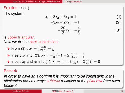
In the previous example the three different norms of A were of similarmagnitude.
RemarkAll matrix norms are equivalent, i.e., comparable in size. In fact, for anym × n matrix A we have
1√n‖A‖∞ ≤ ‖A‖2 ≤
√n‖A‖1,
1√m‖A‖1 ≤ ‖A‖2 ≤
√m‖A‖∞.
ExampleFor the 3× 3 Hilbert matrix this implies:
1√3‖A‖∞ ≤ ‖A‖2 ≤
√3‖A‖1
=⇒ 0.5774× 1.8333︸ ︷︷ ︸=1.0585
≤ ‖A‖2 ≤ 1.7321× 1.8333︸ ︷︷ ︸=3.1754
[email protected] MATH 350 – Chapter 2 37

Roundoff Error and the Condition Number of a Matrix The Condition Number of a Matrix
Definition
The quantity κ(A) = ‖A‖‖A−1‖ is called the condition number of A.
RemarkThe condition number depends on the type of norm used.
For the 2-norm of a nonsingular n × n matrix A we know ‖A‖2 = σ1(the largest singular value of A).Similarly, ‖A−1‖2 = 1
σn(with σn the smallest singular value of A).
Thus,κ(A) = ‖A‖2‖A−1‖2 =
σ1
σn.
Note that κ(A) ≥ 1. In fact, this holds for any norm.
Singular values and the SVD are discussed in detail in MATH 477.
[email protected] MATH 350 – Chapter 2 38

Roundoff Error and the Condition Number of a Matrix The Condition Number of a Matrix
Example
Consider the matrix A =
[0.780 0.5630.913 0.659
]from our earlier example.
Compute κ2(A).
SolutionIn MATLAB we compute the singular values of A with s = svd(A).This yields
σ1 = 1.480952059, σ2 = 0.000000675,
so thatκ2(A) =
σ1
σ2= 2.193218999× 10⁶.
This is very large for a 2× 2 matrix.Note that the latter can be obtained directly with the commandcond(A) in MATLAB.
[email protected] MATH 350 – Chapter 2 39

Roundoff Error and the Condition Number of a Matrix The Condition Number of a Matrix
In order to see what effect the condition number has on the reliability ofthe residual for predicting the accuracy of the solution to the linearsystem we can refer to the following result.
TheoremConsider the linear system Ax = b with computed solution x∗, residualr = b − Ax∗, and exact solution x . Then
1κ(A)
‖r‖‖b‖ ≤
‖x − x∗‖‖x‖ ≤ κ(A) ‖r‖‖b‖ ,
i.e., the relative error is bounded from above and below by the relativeresidual and the condition number of A.
In particular, if the condition number of A is small (close to 1), then asmall residual will accurately predict a small error.
[email protected] MATH 350 – Chapter 2 40

Roundoff Error and the Condition Number of a Matrix The Condition Number of a Matrix
Earlier we used A =
[0.780 0.5630.913 0.659
]with κ2(A) = 2.1932× 10⁶.
For b =
[0.2170.254
](with ‖b‖2 = 0.3341) we had r =
[−0.000460−0.000541
](with
‖r‖2 = 7.1013× 10⁻⁴).The theorem tells us
1κ(A)
‖r‖‖b‖ ≤
‖x−x∗‖‖x‖ ≤ κ(A) ‖r‖‖b‖
=⇒ 12.1932×10⁶
7.1013×10⁻⁴
0.3341 ≤ ‖x−x∗‖‖x‖ ≤ 2.1932× 10⁶ 7.1013×10⁻⁴
0.3341
=⇒ 9.6912× 10⁻¹⁰ ≤ ‖x−x∗‖‖x‖ ≤ 4.6617× 10³.
This estimate ranges over 13 orders of magnitude and tells us thatsince our matrix is ill-conditioned, the residual is totally unreliable.Note that our relative error was‖x − x∗‖‖x‖ =
‖[−0.443,1.00]T − [1,−1]T‖‖[1,−1]T‖ =
2.46621.4142
= 1.7439.
[email protected] MATH 350 – Chapter 2 41

Special Matrices Sparse Matrices
DefinitionA matrix A is called sparse if many of its entries are zero. Otherwise, Ais called dense or full.
The MATLAB command nnz gives the number of nonzero entries in amatrix, and so we can compute
density = nnz(A)/prod(size(A))sparsity = 1 - density
A sparse matrix has very small density (i.e., sparsity close to 1).
An n × n diagonal matrix has density 1/n and sparsity 1− 1/n.
[email protected] MATH 350 – Chapter 2 43

Special Matrices Sparse Matrices
Sparse Matrices in MATLAB
Since it would be a waste to store every single entry in a sparse matrix(many of which are zero), MATLAB has a special data structure to dealwith sparse matrices.
The MATLAB command
S = sparse(i,j,x,m,n)
produces an m × n sparse matrix S whose nonzero entries (specifiedin the vector x) are located at the (i , j) positions (specified in thevectors i and j of row and column indices, respectively).
[email protected] MATH 350 – Chapter 2 44
Special Matrices Sparse Matrices
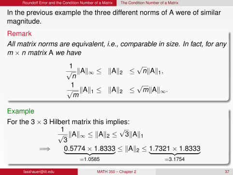
Sparse Matrices in MATLAB (cont.)
Examplei = [1 1 3], j = [1 2 3], x = [1 1 1]S = sparse(i,j,x,3,3)
produces
S =
1 1 00 0 00 0 1
.
A sparse matrix can be converted to the full format by A=full(S),and a full matrix is converted to the sparse format by S=sparse(A).
[email protected] MATH 350 – Chapter 2 45

Special Matrices Sparse Matrices
Algorithms for Sparse Linear Systems
There are two main categories of algorithms to solve linear systemsAx = b when A is sparse.
Direct methods:Especially for tridiagonal or banded systems (see below). Donewith a custom implementation of Gaussian elimination.MATLAB’s built-in solvers (such as the backslash solver) work withthe sparse matrix format.
Iterative methods (discussed in detail in MATH 477):Stationary (“classical”) methods such as Jacobi, Gauss-Seidel orSOR iteration.Krylov subspace methods such as conjugate gradient or GMRES.MATLAB has special routines for these and many others.
An efficient linear solver will always use as much structure of A aspossible.
[email protected] MATH 350 – Chapter 2 46

Special Matrices Sparse Matrices
Jacobi Iteration
ExampleFor the system
2x1 + x2 = 6x1 + 2x2 = 6
the Jacobi method looks like
x (k)1 =
(6− x (k−1)
2
)/2
x (k)2 =
(6− x (k−1)
1
)/2.
We start with an initial guess [x (0)1 , x (0)
2 ]T and then iterate to improvethe answer.
[email protected] MATH 350 – Chapter 2 47

Special Matrices Sparse Matrices
Jacobi Iteration (cont.)
In general,
Jacobi iteration
Let x (0) be an arbitrary initial guessfor k = 1,2, . . .
for i = 1 : m
x (k)i =
bi −i−1∑j=1
aijx(k−1)j −
m∑j=i+1
aijx(k−1)j
/aii
end
end
[email protected] MATH 350 – Chapter 2 48

Special Matrices Sparse Matrices
Gauss-Seidel Iteration
ExampleIn order to improve the Jacobi method we notice that the value ofx (k−1)
1 used in the second equation of the example above is actuallyoutdated since we already computed a newer version, x (k)
1 , in the firstequation.Therefore, we might consider
x (k)1 =
(6− x (k−1)
2
)/2
x (k)2 =
(6− x (k)
1
)/2
instead.This is known as the Gauss-Seidel method.
[email protected] MATH 350 – Chapter 2 49

Special Matrices Sparse Matrices
Gauss-Seidel Iteration (cont.)
The general algorithm is of the form
Gauss-Seidel iteration
Let x (0) be an arbitrary initial guessfor k = 1,2, . . .
for i = 1 : m
x (k)i =
bi −i−1∑j=1
aijx(k)j −
m∑j=i+1
aijx(k−1)j
/aii
end
end
[email protected] MATH 350 – Chapter 2 50

Special Matrices Sparse Matrices
Classical Iterative Solvers
The Jacobi or Gauss-Seidel method are conceptually very easy tounderstand, but are not very useful for solving linear systems.
For example, MATLAB does not have any special code for them.
They are useful, however, in preconditioning given linear systemsfor use with other — more powerful — iterative solvers.
They are also frequently used as preconditioners in domaindecomposition methods.
[email protected] MATH 350 – Chapter 2 51

Special Matrices Sparse Matrices
ExampleThe matrix (A = gallery(’poisson’,3); full(A))
4 −1 0 −1 0 0 0 0 0−1 4 −1 0 −1 0 0 0 00 −1 4 0 0 −1 0 0 0−1 0 0 4 −1 0 −1 0 00 −1 0 −1 4 −1 0 −1 00 0 −1 0 −1 4 0 0 −10 0 0 −1 0 0 4 −1 00 0 0 0 −1 0 −1 4 −10 0 0 0 0 −1 0 −1 4
is a typical sparse matrix that arises in the finite difference solution of(partial) differential equations.Note that all its nonzero entries are close to the diagonal, i.e., it isbanded (see next slide). It is even block tridiagonal.
[email protected] MATH 350 – Chapter 2 52

Special Matrices Banded Matrices
DefinitionA matrix A is called banded if its nonzero entries are all located on themain diagonal as well as neighboring sub- and super-diagonals.
We can determine the bandwidth of A via
[i,j] = find(A) % finds indices of nonzero entriesbandwidth = max(abs(i-j))
ExampleThe finite difference matrix of the previous slide has bandwidth 3.
An n × n diagonal matrix has bandwidth zero.
We will see banded matrices in the context of spline interpolation.
[email protected] MATH 350 – Chapter 2 53

Special Matrices Banded Matrices
Tridiagonal Matrices
A matrix whose upper and lower bandwidth are both 1 is calledtridiagonal. Tridiagonal matrices arise, e.g., when working with splines,finite element, or finite difference methods.A tridiagonal (or more general banded) matrix is usually given byspecifying its diagonals.
The MATLAB command A = gallery(’tridiag’,a,b,c) definesthe matrix
A =
b1 c1 0 . . . 0
a1 b2 c2. . .
...
0. . . . . . . . . 0
.... . . an−2 bn1 cn−1
0 . . . 0 an−1 bn
Note that the vectors a and c specifying the sub- and superdiagonals,respectively, have one entry fewer than the diagonal b.
[email protected] MATH 350 – Chapter 2 54
Special Matrices Banded Matrices
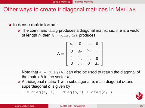
Other ways to create tridiagonal matrices in MATLAB
In dense matrix format:The command diag produces a diagonal matrix, i.e., if a is a vectorof length n, then A = diag(a) produces
A =
a1 0 . . . 0
0 a2. . .
......
. . . . . . 00 . . . 0 an
.Note that a = diag(A) can also be used to return the diagonal ofthe matrix A in the vector a.A tridiagonal matrix T with subdiagonal a, main diagonal b, andsuperdiagonal c is given byT = diag(a,-1) + diag(b,0) + diag(c,1)
[email protected] MATH 350 – Chapter 2 55

Special Matrices Banded Matrices
Other ways to create tridiagonal matrices in MATLAB
(cont.)
In sparse matrix format:An n × n tridiagonal matrix T with subdiagonal a, main diagonal b,and superdiagonal c is given byT = spdiags([a,b,c],[-1 0 1],n,n)
spdiags can also be used to extract the diagonals from a sparsematrix.
In both cases, MATLAB’s built-in backslash operator will solve thelinear system Tx = d efficiently using a direct method.
[email protected] MATH 350 – Chapter 2 56
Special Matrices Banded Matrices
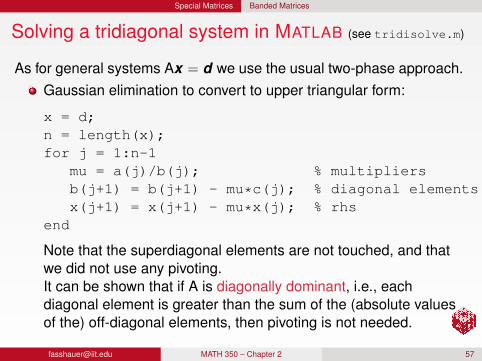
Solving a tridiagonal system in MATLAB (see tridisolve.m)
As for general systems Ax = d we use the usual two-phase approach.Gaussian elimination to convert to upper triangular form:
x = d;n = length(x);for j = 1:n-1
mu = a(j)/b(j); % multipliersb(j+1) = b(j+1) - mu*c(j); % diagonal elementsx(j+1) = x(j+1) - mu*x(j); % rhs
end
Note that the superdiagonal elements are not touched, and thatwe did not use any pivoting.It can be shown that if A is diagonally dominant, i.e., eachdiagonal element is greater than the sum of the (absolute valuesof the) off-diagonal elements, then pivoting is not needed.
[email protected] MATH 350 – Chapter 2 57

Special Matrices Banded Matrices
Solving a tridiagonal system in MATLAB (cont.)
Back substitution:
x(n) = x(n)/b(n);for j = n-1:-1:1
x(j) = (x(j)-c(j)*x(j+1))/b(j);end
The code from this and the previous slide is combined in the functiontridisolve from [NCM].
Remark
Recall that standard Gaussian elimination requires O(n3) operations,and back substitution O(n2). The specialized code tridisolverequires only O(n) operations (see TridisolveDemo.m).
[email protected] MATH 350 – Chapter 2 58

An Application: Google’s Page Rank
A Mathematical Model for the InternetThe following is from Sect. 2.11 of [NCM] (which is based on [Page et al.]).Start with a connectivity matrix G of zeros and ones such that
gij = 1 if page #j links to page #i .
G is n × n, where — for the entire internet — n is huge, i.e., O(1012)(see this Google blog).ExampleConsider a tiny web consisting of only n = 6 webpages:
[email protected] MATH 350 – Chapter 2 60
26 Chapter 2. Linear Equations
Then repeat the statement
x = G*x + e*(z*x)
until x settles down to several decimal places.It is also possible to use an algorithm known as inverse iteration.
A = p*G*D + delta
x = (I - A)\e
x = x/sum(x)
At first glance, this appears to be a very dangerous idea. Because I − A is the-oretically singular, with exact computation some diagonal element of the uppertriangular factor of I − A should be zero and this computation should fail. Butwith roundoff error, the computed matrix I - A is probably not exactly singular.Even if it is singular, roundoff during Gaussian elimination will most likely pre-vent any exact zero diagonal elements. We know that Gaussian elimination withpartial pivoting always produces a solution with a small residual, relative to thecomputed solution, even if the matrix is badly conditioned. The vector obtainedwith the backslash operation, (I - A)\e, usually has very large components. If itis rescaled by its sum, the residual is scaled by the same factor and becomes verysmall. Consequently, the two vectors x and A*x equal each other to within roundofferror. In this setting, solving the singular system with Gaussian elimination blowsup, but it blows up in exactly the right direction.
alpha
beta
gamma
delta
sigma rho
Figure 2.2. A tiny Web.
Figure 2.2 is the graph for a tiny example, with n = 6 instead of n = 4 · 109.Pages on the Web are identified by strings known as uniform resource locators,or URLs. Most URLs begin with http because they use the hypertext transferprotocol. In Matlab , we can store the URLs as an array of strings in a cell array.This example involves a 6-by-1 cell array.
G =
0 0 0 1 0 11 0 0 0 0 00 1 0 0 0 00 1 1 0 0 00 0 1 0 0 01 0 1 0 0 0

An Application: Google’s Page Rank
A Mathematical Model for the Internet (cont.)
In order to simulate web browsing, we use as a mathematical model arandom walk or Markov chain with transition matrix A such that
aij =
{pgijcj
+ δ, cj 6= 0
1/n, cj = 0
where aij denotes the probability of someone going to page #i whenthey’re visiting page #j , and
p is the probability that an existing link is followed (typical valuep = 0.85). Then 1− p is the probability that a random page isvisited instead.cj =
∑nj=1 gij , the column sums of G (called the out-degree of
page #j , i.e., how many pages the j-th page links to).δ = (1− p)/n is the (tiny) probability of going to a particularrandom page.
[email protected] MATH 350 – Chapter 2 61

An Application: Google’s Page Rank
A Mathematical Model for the Internet (cont.)
Example
A=
0.0250 0.0250 0.0250 0.8750 0.1667 0.87500.4500 0.0250 0.0250 0.0250 0.1667 0.02500.0250 0.4500 0.0250 0.0250 0.1667 0.02500.0250 0.4500 0.3083 0.0250 0.1667 0.02500.0250 0.0250 0.3083 0.0250 0.1667 0.02500.4500 0.0250 0.3083 0.0250 0.1667 0.0250
, λ=
1.0000−0.5867
−0.1341 + 0.3882i−0.1341− 0.3882i
0.14650.0000
All our transition matrices havepositive entries, i.e., aij > 0 for all i , j ,column sums equal to one, i.e.,
∑ni=1 aij = 1 for all j ,
their largest eigenvalue equal to one, i.e., λ1 = 1.For such matrices the Perron-Frobenius theorem ensures that
Ax = x ⇐⇒ (A− I)x = 0
has a unique solution x such that∑n
i=1 xi = 1. The vector x is calledthe state vector of A. It is also Google’s page rank vector.
[email protected] MATH 350 – Chapter 2 62

An Application: Google’s Page Rank
A Mathematical Model for the Internet (cont.)
In linear algebra jargon we are trying to find the eigenvector xassociated with the maximum eigenvalue λ1 = 1.The simplest algorithm for doing this (and for huge matrices, such asthe Google matrix, the only feasible method) is:
Power iteration
Initialize x (0) with arbitrary nonzero vector (e.g., x (0) = [1n , . . . ,
1n ])
for k = 1,2, . . .x (k) = Ax (k−1)
end
Run the MATLAB script TinyWeb.m to see the example of this sectionworked through.The [NCM] program surfer can be used to compute page ranksstarting at any URL. Note that this program is a bit buggy and mayeven crash MATLAB.
[email protected] MATH 350 – Chapter 2 63

Appendix References
References I
J. W. Demmel.Applied Numerical Linear Algebra.SIAM, Philiadelphia, 1997.
G. H. Golub and C. Van Loan.Matrix Computations.Johns Hopkins University Press (3rd ed.), Baltimore, 1996.
C. D. Meyer.Matrix Analysis and Applied Linear Algebra .SIAM, Philadelphia, 2000.Also http://www.matrixanalysis.com/.
C. Moler.Numerical Computing with MATLAB.SIAM, Philadelphia, 2004.Also http://www.mathworks.com/moler/.
[email protected] MATH 350 – Chapter 2 64
Appendix References
References II
G. Strang.Introduction to Linear Algebra.Wellesley-Cambridge Press (3rd ed.), Wellesley, MA, 2003.
G. Strang.Linear Algebra and Its Applications.Brooks Cole (4th ed.), 2005.
L. N. Trefethen and D. Bau, III.Numerical Linear Algebra.SIAM, Philadelphia, 1997.
L. Page, S. Brin, R. Motwani, and T. Winograd.The PageRank Citation Ranking: Bringing Order to the Web.http://ilpubs.stanford.edu:8090/422/
M. du Sautoy.The Story of Maths — BBC The Genius of the East.click here
[email protected] MATH 350 – Chapter 2 65

Appendix References
References III
G. Strang.Video lectures of Gilbert Strang teaching MIT’s Linear Algebra 18.06.http://ocw.mit.edu/OcwWeb/Mathematics/18-06Spring-2005/VideoLectures/index.htm
[email protected] MATH 350 – Chapter 2 66