Embed Size (px)
Citation preview
MATLAB SIMULINK ® - Simulation and Model Based Design
http://www.mathworks.com
What is Simulink good for?
-Modeling/designing dynamic systems (including nonlinear dynamics)
-Modeling/designing control systems (including nonlinear controllers and plants)
-Signal processing design/simulation
Simulink runs under Matlab. First
start Matlab, then type “simulink” at the Matlab prompt.
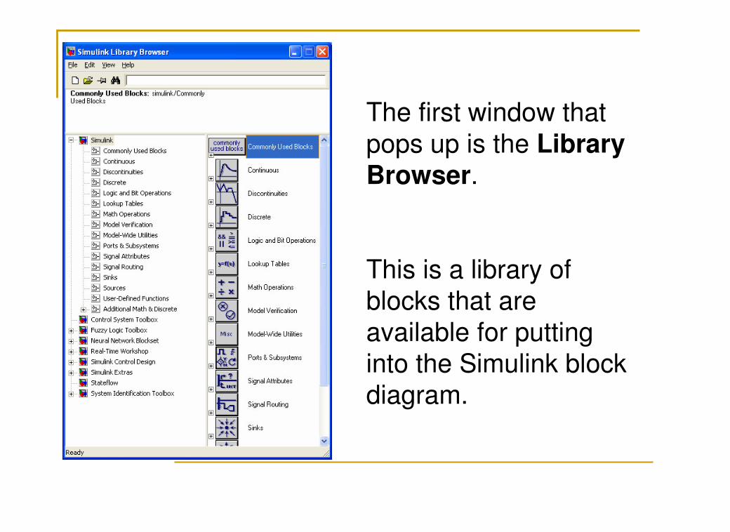
The first window that
pops up is the Library
Browser.
This is a library of
blocks that are
available for putting
into the Simulink block
diagram.
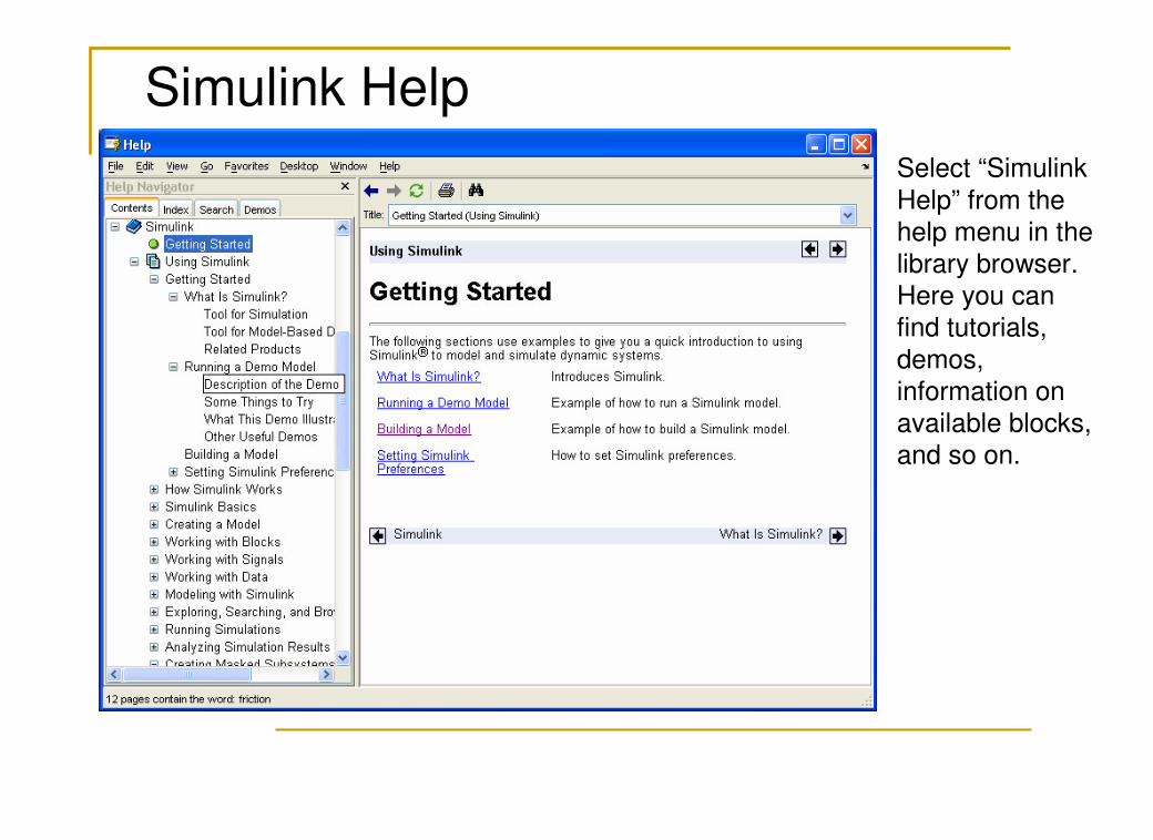
Simulink Help
Select “Simulink
Help” from the
help menu in the library browser.
Here you can
find tutorials,
demos,
information on
available blocks,
and so on.

A Simulink model is a block diagram. Click “File|New|Model” in the Library Browser. An empty block diagram will pop up. You can drag blocks into the diagram from the library.
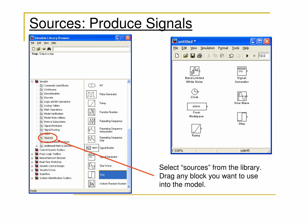
Sources: Produce Signals
Select “sources” from the library.
Drag any block you want to use
into the model.
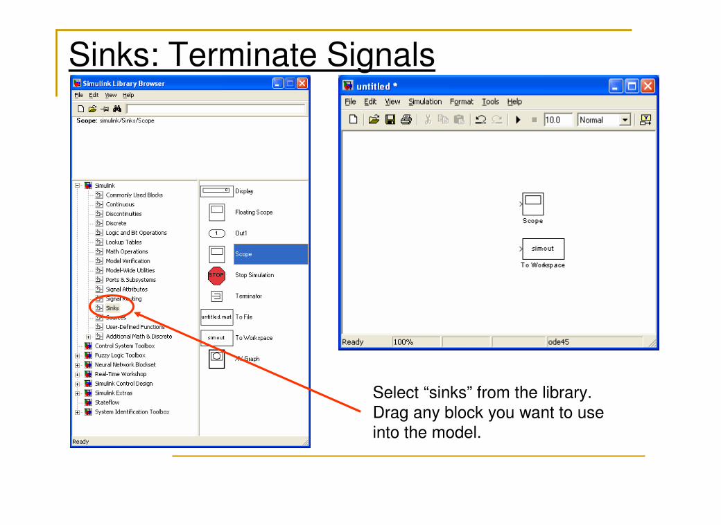
Sinks: Terminate Signals
Select “sinks” from the library.
Drag any block you want to use
into the model.
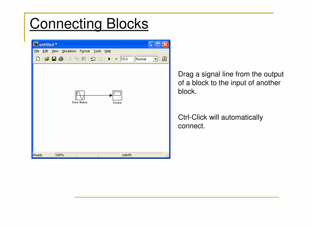
Connecting Blocks
Drag a signal line from the output
of a block to the input of another
block.
Ctrl-Click will automatically
connect.
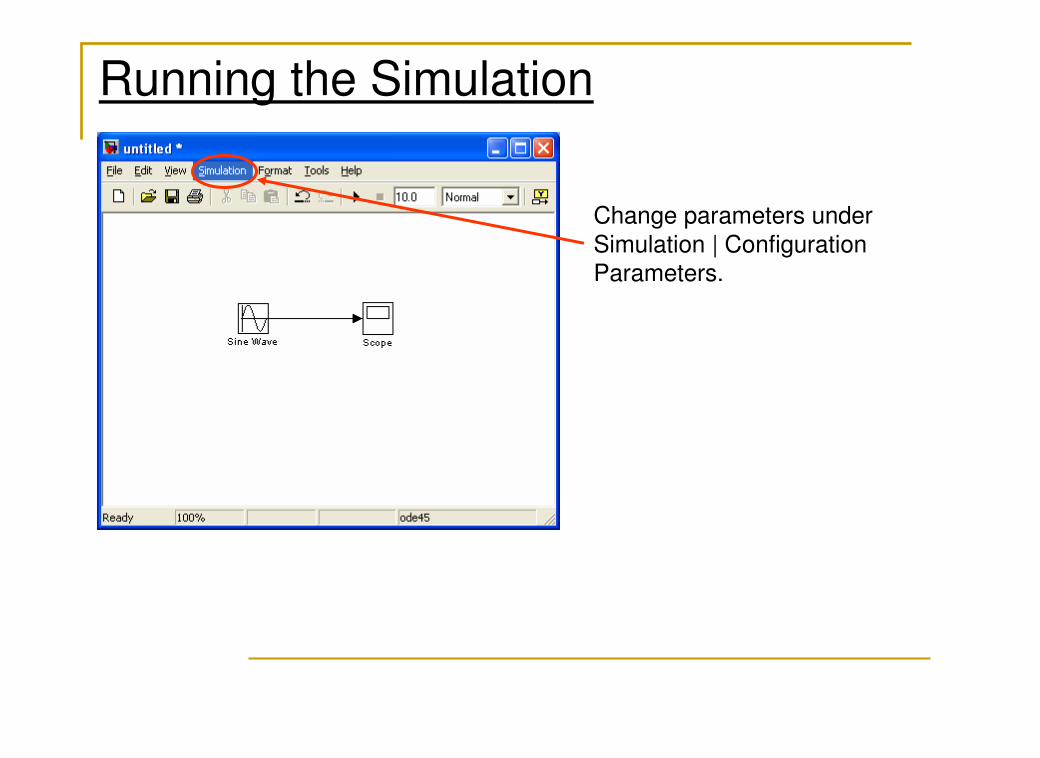
Running the Simulation
Change parameters under
Simulation | Configuration
Parameters.
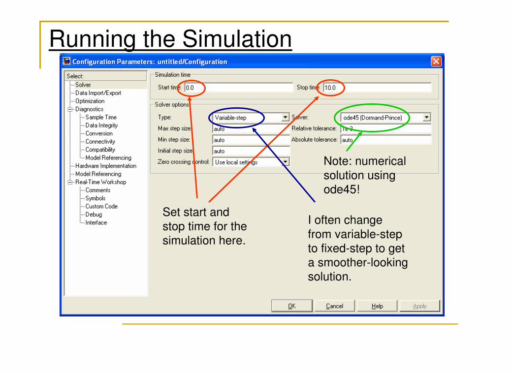
Running the Simulation
Set start and
stop time for the
simulation here.
I often change
from variable-step
to fixed-step to get a smoother-looking
solution.
Note: numerical
solution using
ode45!
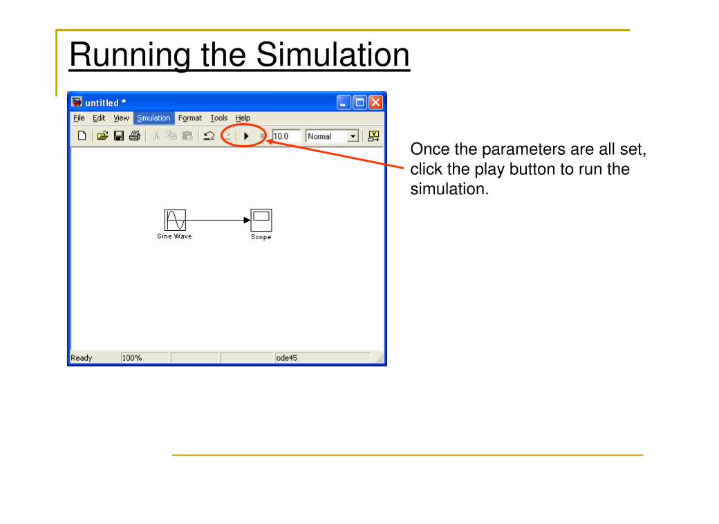
Running the Simulation
Once the parameters are all set,
click the play button to run the
simulation.
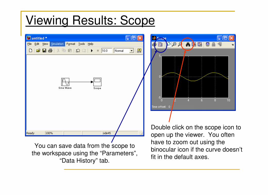
Viewing Results: Scope
Double click on the scope icon to
open up the viewer. You often have to zoom out using the
binocular icon if the curve doesn’t
fit in the default axes.
You can save data from the scope to
the workspace using the “Parameters”,
“Data History” tab.
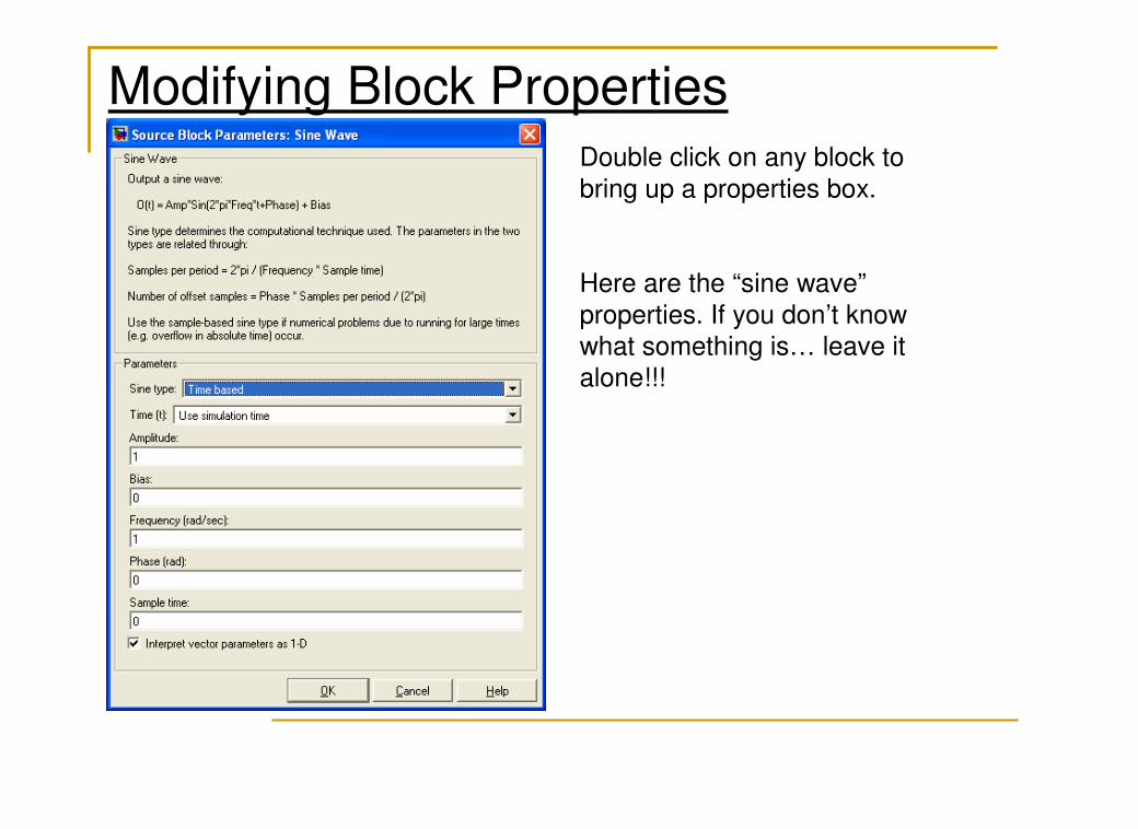
Modifying Block PropertiesDouble click on any block to
bring up a properties box.
Here are the “sine wave”
properties. If you don’t know what something is… leave it alone!!!
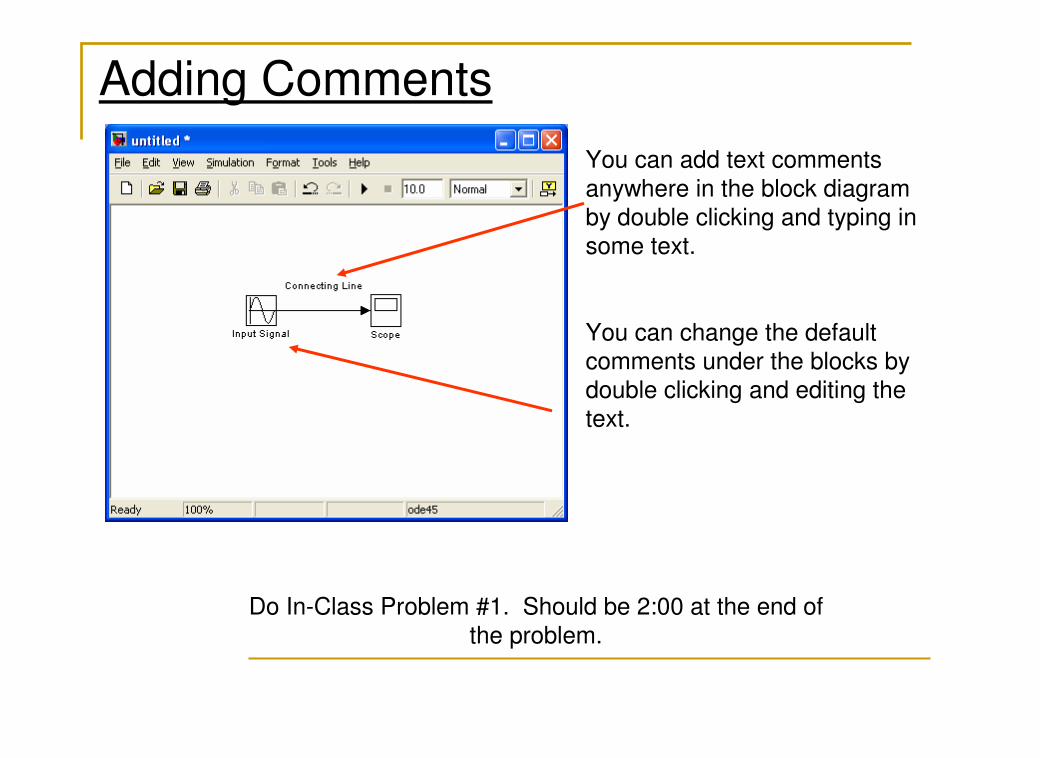
Adding Comments
You can add text comments
anywhere in the block diagram
by double clicking and typing in some text.
You can change the default
comments under the blocks by
double clicking and editing the
text.
Do In-Class Problem #1. Should be 2:00 at the end of
the problem.
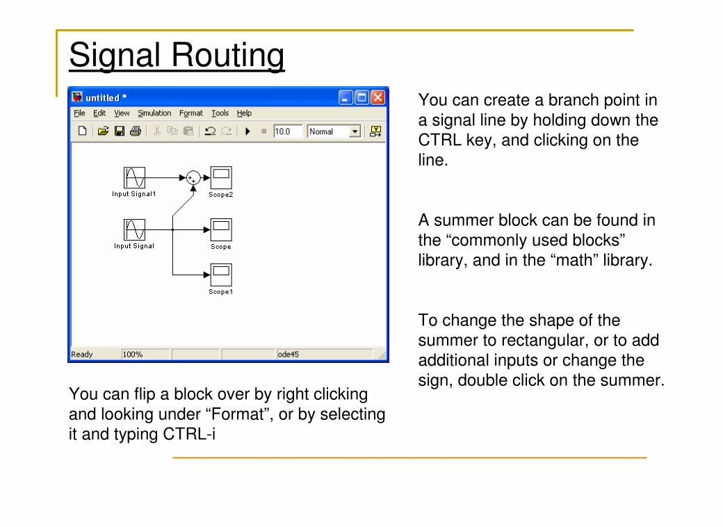
Signal RoutingYou can create a branch point in
a signal line by holding down the
CTRL key, and clicking on the line.
A summer block can be found in
the “commonly used blocks”
library, and in the “math” library.
To change the shape of the
summer to rectangular, or to add
additional inputs or change the sign, double click on the summer.
You can flip a block over by right clicking
and looking under “Format”, or by selecting
it and typing CTRL-i
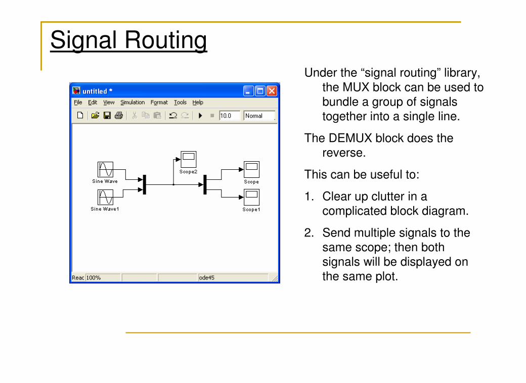
Signal RoutingUnder the “signal routing” library,
the MUX block can be used to
bundle a group of signals together into a single line.
The DEMUX block does the reverse.
This can be useful to:
1. Clear up clutter in a
complicated block diagram.
2. Send multiple signals to the
same scope; then both
signals will be displayed on the same plot.
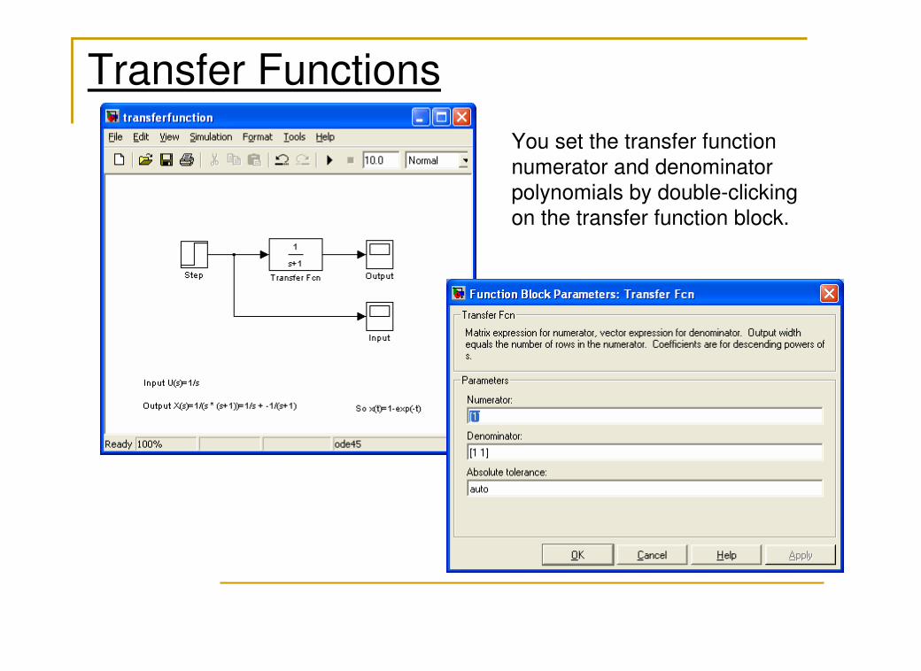
Transfer Functions
You set the transfer function
numerator and denominator
polynomials by double-clicking on the transfer function block.
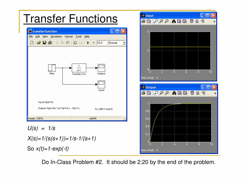
Transfer Functions
U(s) = 1/s
X(s)=1/(s(s+1))=1/s-1/(s+1)
So x(t)=1-exp(-t)
Do In-Class Problem #2. It should be 2:20 by the end of the problem.
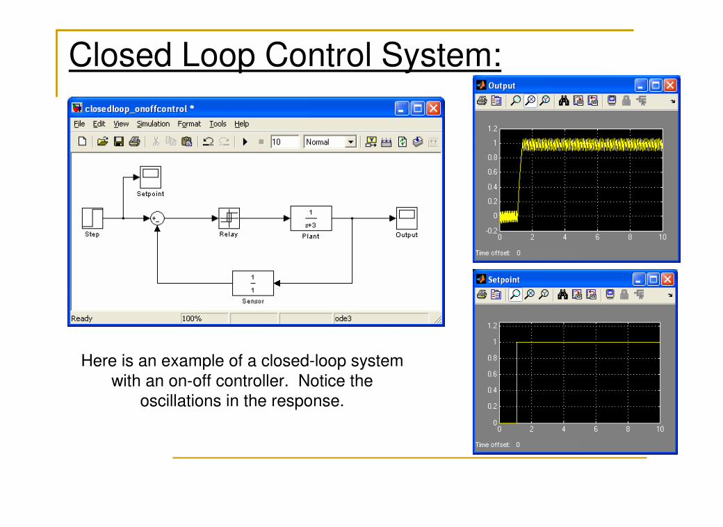
Closed Loop Control System:
Here is an example of a closed-loop system
with an on-off controller. Notice the
oscillations in the response.
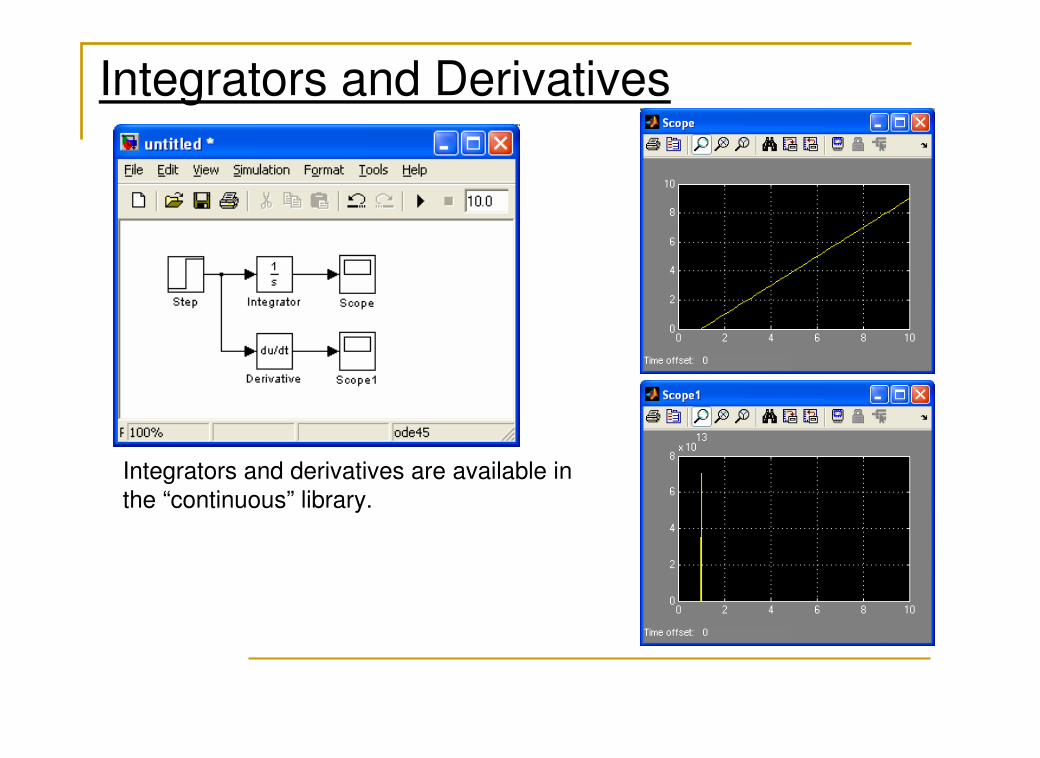
Integrators and Derivatives
Integrators and derivatives are available in
the “continuous” library.
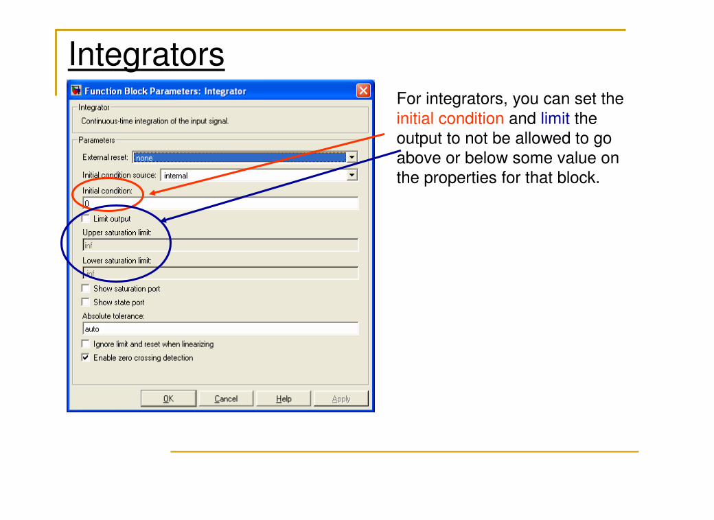
IntegratorsFor integrators, you can set the
initial condition and limit the
output to not be allowed to go above or below some value on
the properties for that block.
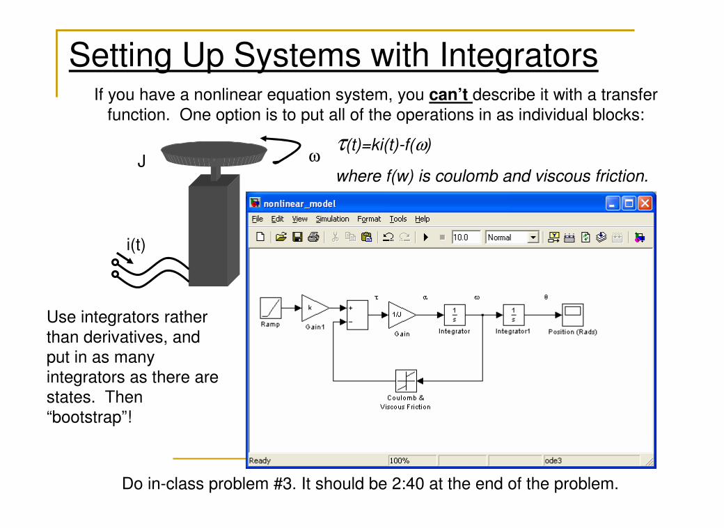
Setting Up Systems with IntegratorsIf you have a nonlinear equation system, you can’t describe it with a transfer
function. One option is to put all of the operations in as individual blocks:
ω
i(t)
Jτ(t)=ki(t)-f(ω)
where f(w) is coulomb and viscous friction.
Use integrators rather
than derivatives, and
put in as many integrators as there are
states. Then
“bootstrap”!
Do in-class problem #3. It should be 2:40 at the end of the problem.
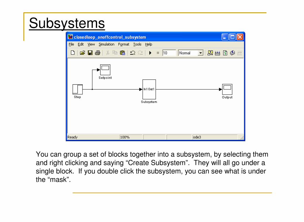
Subsystems
You can group a set of blocks together into a subsystem, by selecting them
and right clicking and saying “Create Subsystem”. They will all go under a
single block. If you double click the subsystem, you can see what is under
the “mask”.
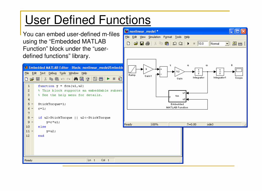
User Defined FunctionsYou can embed user-defined m-files
using the “Embedded MATLAB
Function” block under the “user-defined functions” library.
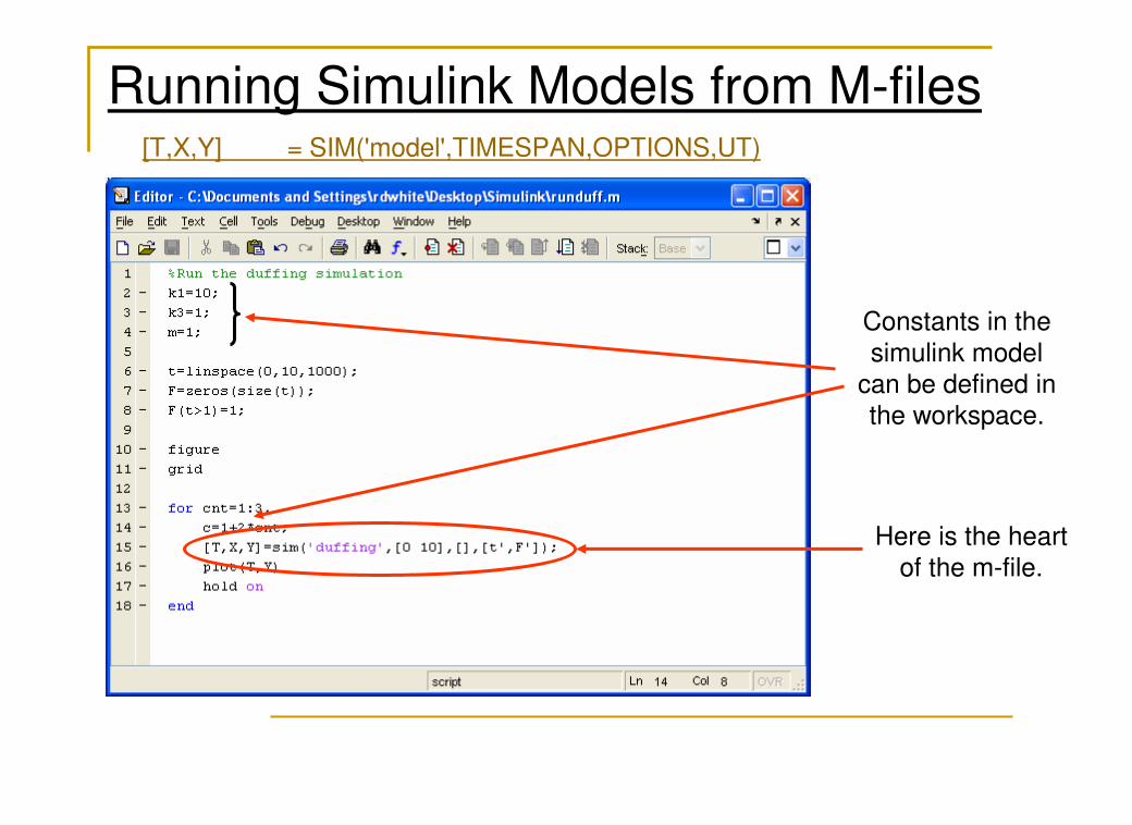
Running Simulink Models from M-files[T,X,Y] = SIM('model',TIMESPAN,OPTIONS,UT)
Here is the heart
of the m-file.
Constants in the
simulink model can be defined in
the workspace.
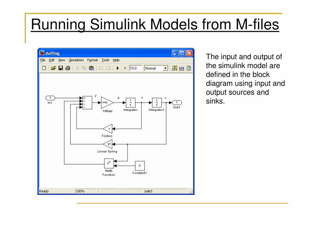
Running Simulink Models from M-files
The input and output of
the simulink model are
defined in the block diagram using input and
output sources and
sinks.
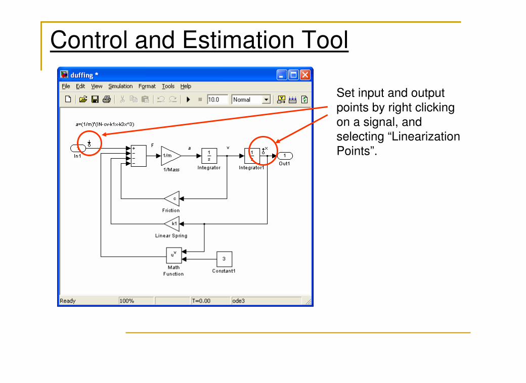
Control and Estimation Tool
Set input and output
points by right clicking
on a signal, and selecting “Linearization
Points”.
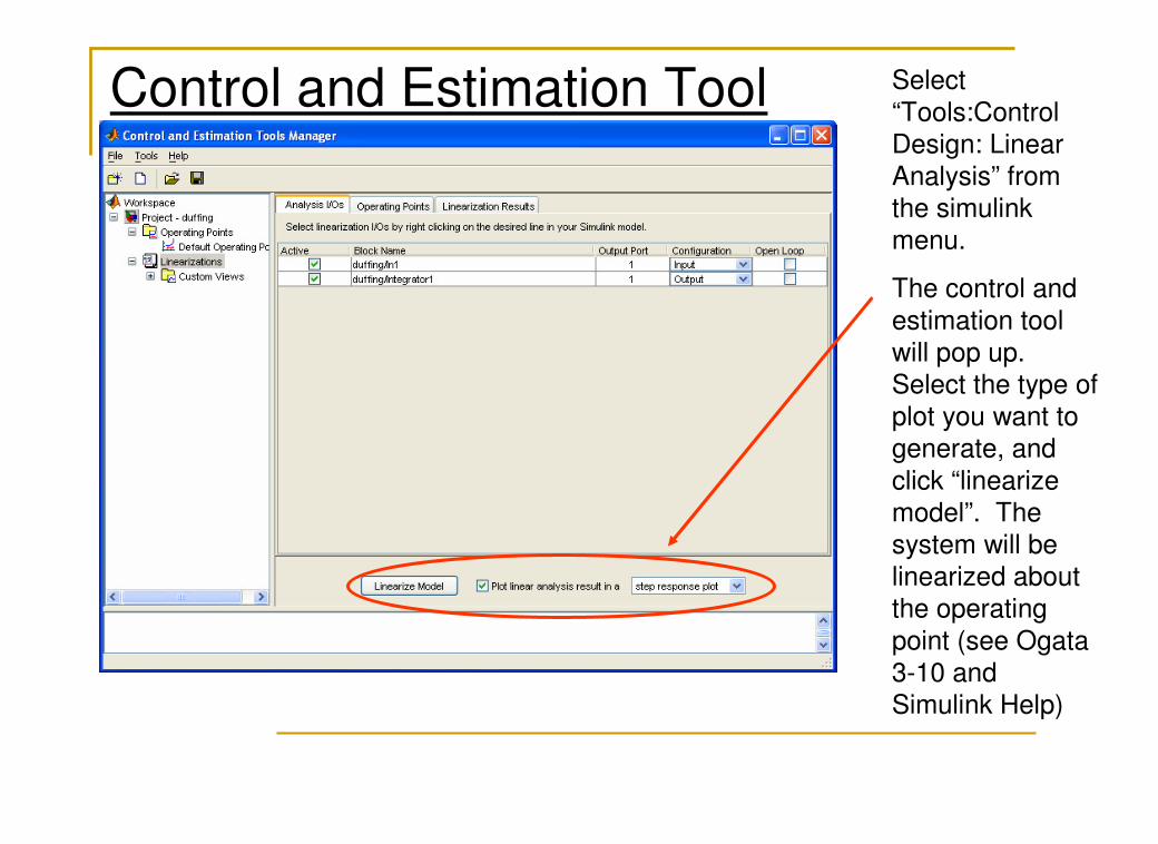
Control and Estimation Tool Select
“Tools:ControlDesign: Linear Analysis” from
the simulink
menu.
The control and
estimation tool will pop up. Select the type of
plot you want to
generate, and
click “linearize
model”. The
system will be
linearized about the operating
point (see Ogata
3-10 and Simulink Help)
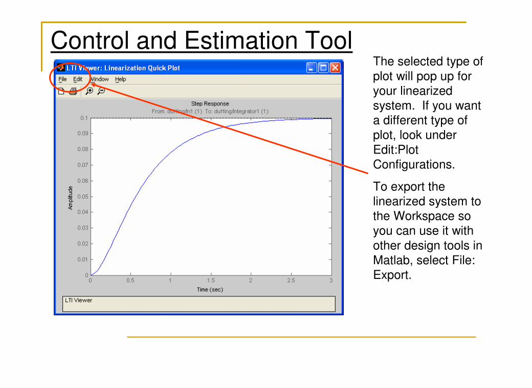
Control and Estimation ToolThe selected type of
plot will pop up for
your linearizedsystem. If you want
a different type of
plot, look under
Edit:Plot
Configurations.
To export the
linearized system to
the Workspace so you can use it with
other design tools in
Matlab, select File: Export.
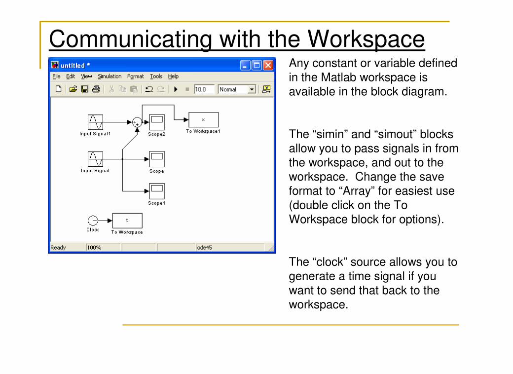
Communicating with the WorkspaceAny constant or variable defined
in the Matlab workspace is
available in the block diagram.
The “simin” and “simout” blocks
allow you to pass signals in from
the workspace, and out to the workspace. Change the save
format to “Array” for easiest use
(double click on the To Workspace block for options).
The “clock” source allows you to
generate a time signal if you
want to send that back to the
workspace.
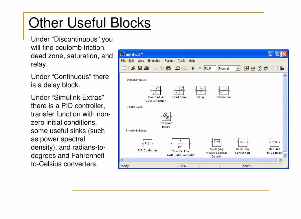
Other Useful BlocksUnder “Discontinuous” you
will find coulomb friction,
dead zone, saturation, and relay.
Under “Continuous” there is a delay block.
Under “Simulink Extras”
there is a PID controller,
transfer function with non-
zero initial conditions, some useful sinks (such
as power spectral
density), and radians-to-degrees and Fahrenheit-
to-Celsius converters.