RF Basics

Martin D. Stoehr PMTS, ISM-RF Strategic Applications

Page 2 of 55

Table of Contents Table of Contents .............................................................................................................................................................................. 2 Introduction ...................................................................................................................................................................................... 2 History (How Do We Know What We Know?) .................................................................................................................................. 3

Transmitter .......................................................................................................................................................................................................... 4 Receiver ............................................................................................................................................................................................................... 5 Transceiver ........................................................................................................................................................................................................... 5

What Is RF? ....................................................................................................................................................................................... 6 RF Glossary ....................................................................................................................................................................................... 7

Amplitude and Power .......................................................................................................................................................................................... 7 Field Strength ....................................................................................................................................................................................................... 7 Frequency Domain ............................................................................................................................................................................................... 8 Industry and Protocol Terms .............................................................................................................................................................................. 10 Instruments ........................................................................................................................................................................................................ 12 Matching Terms ................................................................................................................................................................................................. 13 Modulation ........................................................................................................................................................................................................ 16 Radiation, Propagation, and Attenuation........................................................................................................................................................... 18 Radio Blocks ....................................................................................................................................................................................................... 20 Radio Specifications and Operational Terms ...................................................................................................................................................... 26 Time and Frequency ........................................................................................................................................................................................... 33

Who Controls the Use of Radios? ................................................................................................................................................... 35 Regulating Bodies............................................................................................................................................................................................... 35 Standards Organizations .................................................................................................................................................................................... 36 Certifications ...................................................................................................................................................................................................... 37

Where Do I Start for a Radio Design? ............................................................................................................................................. 38 What Frequency Should I Use? (ISM and Other Bands) ..................................................................................................................................... 38 One-Way and Two-Way Systems ....................................................................................................................................................................... 39 Modulation ........................................................................................................................................................................................................ 39 Cost .................................................................................................................................................................................................................... 40 Antenna ............................................................................................................................................................................................................. 40 Power Supply ..................................................................................................................................................................................................... 41 Range ................................................................................................................................................................................................................. 43 Protocols ............................................................................................................................................................................................................ 44 Common Applications ........................................................................................................................................................................................ 44 Tradeoffs ............................................................................................................................................................................................................ 45

Maxim Products .............................................................................................................................................................................. 46 Examples ......................................................................................................................................................................................... 47

Guidelines .......................................................................................................................................................................................................... 47 Application-Specific Reference Designs ............................................................................................................................................................. 47

For More Information ..................................................................................................................................................................... 49 FCC ..................................................................................................................................................................................................................... 50

References ...................................................................................................................................................................................... 50 Index ............................................................................................................................................................................................... 53

Introduction Radio frequency (RF) can be a complex subject to navigate, but it does not have to be. If you are just getting started with radios or maybe you cannot find that old reference book about antenna aperture, this guide can help. It is intended to provide a basic understanding of RF technology, as well act as a quick reference for those who “know their stuff” but may be looking to brush up on that one niche term that they never quite understood. This document is also a useful reference for Maxim’s products and data sheets, an index to deeper analysis found in our application notes, and a general reference for all things RF.

Page 3 of 55

History (How Do We Know What We Know?)

“If I have seen a little further, it is by standing on the shoulders of Giants.”[1] –Isaac Newton

The wireless radio technology that is so ubiquitous today is relatively new. However, there is a long and rich background that leads to our modern knowledge. The very first investigations of what we now call the RF spectrum came from early experiments in optics, electricity, and magnetism. The behavior of light was studied as far back as ancient Greece by Plato, Euclid, Ptolemy, and many others, eventually leading to Newton in the late 17th Century. From ancient triboelectric materials and chemical batteries, various theories of electricity were eventually developed by Coulomb, Volta, and Gauss. Likewise, lode stones from ancient China birthed early theories for magnetism from Kuo and Gilbert, eventually propelling the investigations of Ampere and again, Gauss. Before the early 19th Century, electricity and magnetism were seen as separate forces. However, in 1820 Ørsted found that electric currents exerted a force on magnets, and in 1831 Faraday determined that changes in a magnetic field could induce electrical currents. In 1839, further experiments in electricity led Faraday to show that voltaic electricity (chemical battery), static electricity (triboelectric charge), and magnetically induced currents were all manifestations of the same phenomenon. In 1864, Maxwell combined these discoveries in his paper, “A Dynamical Theory of the Electromagnetic Field,”[2] ushering in our modern understanding of the subject:

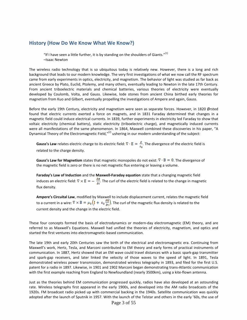
Gauss’s Law relates electric charge to its electric field: . The divergence of the electric field is

related to the charge density. Gauss’s Law for Magnetism states that magnetic monopoles do not exist: . The divergence of the magnetic field is zero or there is no net magnetic flux entering or leaving a volume. Faraday’s Law of Induction and the Maxwell-Faraday equation state that a changing magnetic field induces an electric field: . The curl of the electric field is related to the change in magnetic flux density. Ampere’s Circuital Law, modified by Maxwell to include displacement current, relates the magnetic field to a current in a wire: . The curl of the magnetic flux density is related to the current density and the change in the electric field.

These four concepts formed the basis of electrodynamics or modern-day electromagnetic (EM) theory, and are referred to as Maxwell’s Equations. Maxwell had unified the theories of electricity, magnetism, and optics and started the first ventures into electromagnetic-based communication. The late 19th and early 20th Centuries saw the birth of the electrical and electromagnetic era. Continuing from Maxwell’s work, Hertz, Tesla, and Marconi contributed to EM theory and early forms of practical instruments of communication. In 1887, Hertz showed that an EM wave could travel distances with a basic spark-gap transmitter and spark-gap receivers, and later linked the velocity of those waves to the speed of light. In 1891, Tesla demonstrated wireless power transmission, demonstrated wireless telegraphy in 1893, and filed for the first U.S. patent for a radio in 1897. Likewise, in 1901 and 1902 Marconi began demonstrating trans-Atlantic communication with the first example reaching from England to Newfoundland (nearly 3500km), using a kite-flown antenna. Just as the theories behind EM communication progressed quickly, radios have also developed at an astounding rate. Wireless telegraphs first appeared in the early 1900s, and developed into the AM radio broadcasts of the 1920s. FM broadcast radio picked up with commercial backing in the 1940s. Satellite communication was quickly adopted after the launch of Sputnik in 1957. With the launch of the Telstar and others in the early ’60s, the use of

Page 4 of 55

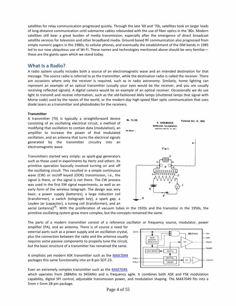
satellites for relay communication progressed quickly. Through the late ’60 and ’70s, satellites took on larger loads of long-distance communication until submarine cables rebounded with the use of fiber optics in the ’80s. Modern satellites still bear a great burden of media transmission, especially after the emergence of direct broadcast satellite services for television and other broadband media. Ground-based RF communication also progressed from simple numeric pagers in the 1980s, to cellular phones, and eventually the establishment of the ISM bands in 1985 led to our now ubiquitous use of Wi-Fi. These names and technologies mentioned above should be very familiar—these are the giants upon which we stand today. What Is a Radio? A radio system usually includes both a source of an electromagnetic wave and an intended destination for that message. The source radio is referred to as the transmitter, while the destination radio is called the receiver. There are occasions where only the receiver is required, such as in radio astronomy. Similarly, home lighting can represent an example of an optical transmitter (usually your eyes would be the receiver, and you are usually receiving reflected signals). A digital camera would be an example of an optical receiver. Occasionally we do use light to transmit and receive information, such as the old-fashioned Aldis lamps (shuttered lamps that signal with Morse code) used by the navies of the world, or the modern-day high-speed fiber optic communication that uses diode lasers as a transmitter and photodiodes for the receivers. Transmitter A transmitter (TX) is typically a straightforward device consisting of an oscillating electrical circuit, a method of modifying that oscillation to contain data (modulation), an amplifier to increase the power of that modulated oscillation, and an antenna that turns the electrical signals generated by the transmitter circuitry into an electromagnetic wave. Transmitters started very simply: as spark-gap generators such as those used in experiments by Hertz and others. Its primitive operation basically involved turning on and off the oscillating circuit. This resulted in a simple continuous wave (CW) or on/off keyed (OOK) transmission, i.e., the signal is there, or the signal is not there. The CW process was used in the first EM signal experiments, as well as an early form of the wireless telegraph. The design was very basic: a power supply (batteries), a large induction coil (transformer), a switch (telegraph key), a spark gap, a Leyden Jar (capacitor), a tuning coil (transformer), and an aerial (antenna)[3]. With the proliferation of vacuum tubes in the 1920s and the transistor in the 1950s, the primitive oscillating system grew more complex, but the concepts remained the same. The parts of a modern transmitter consist of a reference oscillator or frequency source, modulator, power amplifier (PA), and an antenna. There is of course a need for external parts such as a power supply and an oscillation crystal, plus the connection between the radio and the antenna usually requires some passive components to properly tune the circuit, but the basic structure of a transmitter has remained the same. A simplistic yet modern ASK transmitter such as the MAX7044 packages this same functionality into an 8-pin SOT-23. Even an extremely complex transmitter such as the MAX7049, which operates from 288MHz to 945MHz and is frequency agile. It combines both ASK and FSK modulation capability, digital SPI control, adjustable transmission power, and modulation shaping. The MAX7049 fits into a 5mm × 5mm 28-pin package.

Page 5 of 55

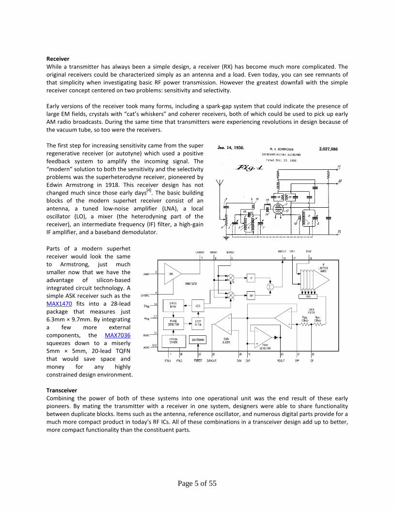
Receiver While a transmitter has always been a simple design, a receiver (RX) has become much more complicated. The original receivers could be characterized simply as an antenna and a load. Even today, you can see remnants of that simplicity when investigating basic RF power transmission. However the greatest downfall with the simple receiver concept centered on two problems: sensitivity and selectivity. Early versions of the receiver took many forms, including a spark-gap system that could indicate the presence of large EM fields, crystals with “cat’s whiskers” and coherer receivers, both of which could be used to pick up early AM radio broadcasts. During the same time that transmitters were experiencing revolutions in design because of the vacuum tube, so too were the receivers. The first step for increasing sensitivity came from the super regenerative receiver (or autotyne) which used a positive feedback system to amplify the incoming signal. The “modern” solution to both the sensitivity and the selectivity problems was the superheterodyne receiver, pioneered by Edwin Armstrong in 1918. This receiver design has not changed much since those early days[4]. The basic building blocks of the modern superhet receiver consist of an antenna, a tuned low-noise amplifier (LNA), a local oscillator (LO), a mixer (the heterodyning part of the receiver), an intermediate frequency (IF) filter, a high-gain IF amplifier, and a baseband demodulator. Parts of a modern superhet receiver would look the same to Armstrong, just much smaller now that we have the advantage of silicon-based integrated circuit technology. A simple ASK receiver such as the MAX1470 fits into a 28-lead package that measures just 6.3mm × 9.7mm. By integrating a few more external components, the MAX7036 squeezes down to a miserly 5mm × 5mm, 20-lead TQFN that would save space and money for any highly constrained design environment. Transceiver Combining the power of both of these systems into one operational unit was the end result of these early pioneers. By mating the transmitter with a receiver in one system, designers were able to share functionality between duplicate blocks. Items such as the antenna, reference oscillator, and numerous digital parts provide for a much more compact product in today’s RF ICs. All of these combinations in a transceiver design add up to better, more compact functionality than the constituent parts.

Page 6 of 55

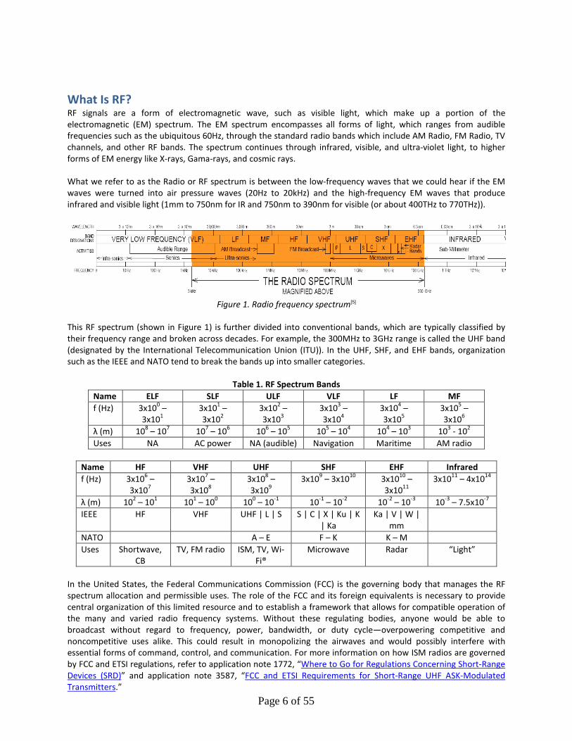
What Is RF? RF signals are a form of electromagnetic wave, such as visible light, which make up a portion of the electromagnetic (EM) spectrum. The EM spectrum encompasses all forms of light, which ranges from audible frequencies such as the ubiquitous 60Hz, through the standard radio bands which include AM Radio, FM Radio, TV channels, and other RF bands. The spectrum continues through infrared, visible, and ultra-violet light, to higher forms of EM energy like X-rays, Gama-rays, and cosmic rays. What we refer to as the Radio or RF spectrum is between the low-frequency waves that we could hear if the EM waves were turned into air pressure waves (20Hz to 20kHz) and the high-frequency EM waves that produce infrared and visible light (1mm to 750nm for IR and 750nm to 390nm for visible (or about 400THz to 770THz)).

Figure 1. Radio frequency spectrum[5]

This RF spectrum (shown in Figure 1) is further divided into conventional bands, which are typically classified by their frequency range and broken across decades. For example, the 300MHz to 3GHz range is called the UHF band (designated by the International Telecommunication Union (ITU)). In the UHF, SHF, and EHF bands, organization such as the IEEE and NATO tend to break the bands up into smaller categories.

Table 1. RF Spectrum Bands Name ELF SLF ULF VLF LF MF f (Hz) 3x100 –

3x101 3x101 – 3x102

3x102 – 3x103

3x103 – 3x104

3x104 – 3x105

3x105 – 3x106

λ (m) 108 – 107 107 – 106 106 – 105 105 – 104 104 – 103 103 - 102 Uses NA AC power NA (audible) Navigation Maritime AM radio

Name HF VHF UHF SHF EHF Infrared f (Hz) 3x106 –

3x107 3x107 – 3x108

3x108 – 3x109

3x109 – 3x1010 3x1010 – 3x1011

3x1011 – 4x1014

λ (m) 102 – 101 101 – 100 100 – 10-1 10-1 – 10-2 10-2 – 10-3 10-3 – 7.5x10-7 IEEE HF VHF UHF | L | S S | C | X | Ku | K

| Ka Ka | V | W |

mm

NATO A – E F – K K – M Uses Shortwave,

CB TV, FM radio ISM, TV, Wi-

Fi® Microwave Radar “Light”

In the United States, the Federal Communications Commission (FCC) is the governing body that manages the RF spectrum allocation and permissible uses. The role of the FCC and its foreign equivalents is necessary to provide central organization of this limited resource and to establish a framework that allows for compatible operation of the many and varied radio frequency systems. Without these regulating bodies, anyone would be able to broadcast without regard to frequency, power, bandwidth, or duty cycle—overpowering competitive and noncompetitive uses alike. This could result in monopolizing the airwaves and would possibly interfere with essential forms of command, control, and communication. For more information on how ISM radios are governed by FCC and ETSI regulations, refer to application note 1772, “Where to Go for Regulations Concerning Short-Range Devices (SRD)” and application note 3587, “FCC and ETSI Requirements for Short-Range UHF ASK-Modulated Transmitters.”

Page 7 of 55

RF Glossary Amplitude and Power

V – Voltage: In RF systems, the voltage of a signal is typically referenced to a 50Ω load. P – Power: In an RF system, power is typically referenced to a 50Ω load.

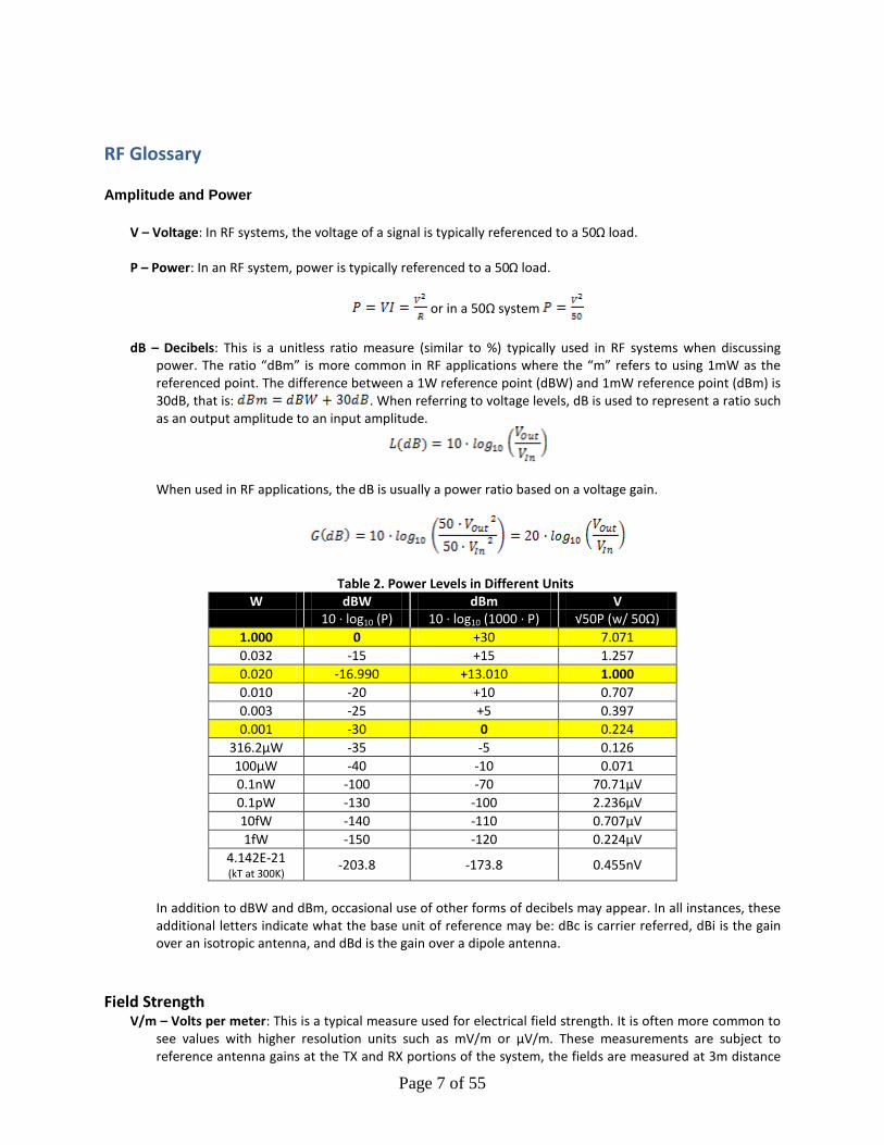
or in a 50Ω system dB – Decibels: This is a unitless ratio measure (similar to %) typically used in RF systems when discussing

power. The ratio “dBm” is more common in RF applications where the “m” refers to using 1mW as the referenced point. The difference between a 1W reference point (dBW) and 1mW reference point (dBm) is 30dB, that is: . When referring to voltage levels, dB is used to represent a ratio such as an output amplitude to an input amplitude.

When used in RF applications, the dB is usually a power ratio based on a voltage gain.

Table 2. Power Levels in Different Units W dBW dBm V

10 · log10 (P) 10 · log10 (1000 · P) √50P (w/ 50Ω) 1.000 0 +30 7.071 0.032 -15 +15 1.257 0.020 -16.990 +13.010 1.000 0.010 -20 +10 0.707 0.003 -25 +5 0.397 0.001 -30 0 0.224

316.2µW -35 -5 0.126 100µW -40 -10 0.071 0.1nW -100 -70 70.71µV 0.1pW -130 -100 2.236µV 10fW -140 -110 0.707µV 1fW -150 -120 0.224µV

4.142E-21 (kT at 300K) -203.8 -173.8 0.455nV

In addition to dBW and dBm, occasional use of other forms of decibels may appear. In all instances, these additional letters indicate what the base unit of reference may be: dBc is carrier referred, dBi is the gain over an isotropic antenna, and dBd is the gain over a dipole antenna.

Field Strength

V/m – Volts per meter: This is a typical measure used for electrical field strength. It is often more common to see values with higher resolution units such as mV/m or µV/m. These measurements are subject to reference antenna gains at the TX and RX portions of the system, the fields are measured at 3m distance

Page 8 of 55

(FCC specified7), and are dependent upon the operating frequency (refer to application note 3815, “Radiated Power and Field Strength from UHF ISM Transmitters” for more information).

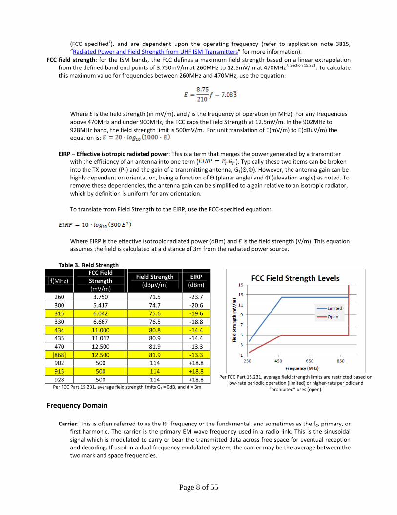
FCC field strength: for the ISM bands, the FCC defines a maximum field strength based on a linear extrapolation from the defined band end points of 3.750mV/m at 260MHz to 12.5mV/m at 470MHz7, Section 15.231. To calculate this maximum value for frequencies between 260MHz and 470MHz, use the equation:

Where E is the field strength (in mV/m), and f is the frequency of operation (in MHz). For any frequencies above 470MHz and under 900MHz, the FCC caps the Field Strength at 12.5mV/m. In the 902MHz to 928MHz band, the field strength limit is 500mV/m. For unit translation of E(mV/m) to E(dBuV/m) the equation is:

EIRP – Effective isotropic radiated power: This is a term that merges the power generated by a transmitter with the efficiency of an antenna into one term ( ). Typically these two items can be broken into the TX power (PT) and the gain of a transmitting antenna, GT(Θ,Φ). However, the antenna gain can be highly dependent on orientation, being a function of Θ (planar angle) and Φ (elevation angle) as noted. To remove these dependencies, the antenna gain can be simplified to a gain relative to an isotropic radiator, which by definition is uniform for any orientation.

To translate from Field Strength to the EIRP, use the FCC-specified equation:

Where EIRP is the effective isotropic radiated power (dBm) and E is the field strength (V/m). This equation assumes the field is calculated at a distance of 3m from the radiated power source.

Table 3. Field Strength

f(MHz) FCC Field Strength (mV/m)

Field Strength (dBµV/m)

EIRP (dBm)

260 3.750 71.5 -23.7 300 5.417 74.7 -20.6 315 6.042 75.6 -19.6 330 6.667 76.5 -18.8 434 11.000 80.8 -14.4 435 11.042 80.9 -14.4 470 12.500 81.9 -13.3

[868] 12.500 81.9 -13.3 902 500 114 +18.8 915 500 114 +18.8 928 500 114 +18.8

Per FCC Part 15.231, average field strength limits GT = 0dB, and d = 3m.

Per FCC Part 15.231, average field strength limits are restricted based on

low-rate periodic operation (limited) or higher-rate periodic and “prohibited” uses (open).

Frequency Domain

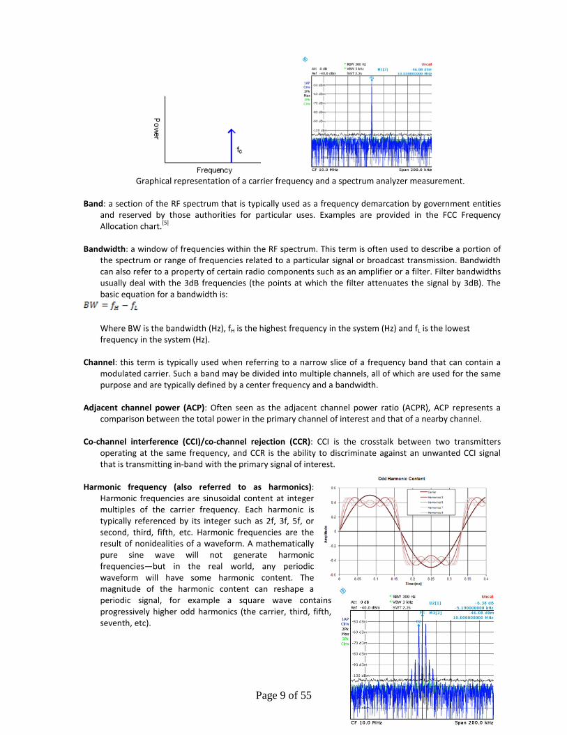
Carrier: This is often referred to as the RF frequency or the fundamental, and sometimes as the fC, primary, or first harmonic. The carrier is the primary EM wave frequency used in a radio link. This is the sinusoidal signal which is modulated to carry or bear the transmitted data across free space for eventual reception and decoding. If used in a dual-frequency modulated system, the carrier may be the average between the two mark and space frequencies.

Page 9 of 55

Graphical representation of a carrier frequency and a spectrum analyzer measurement.

Band: a section of the RF spectrum that is typically used as a frequency demarcation by government entities

and reserved by those authorities for particular uses. Examples are provided in the FCC Frequency Allocation chart.[5]

Bandwidth: a window of frequencies within the RF spectrum. This term is often used to describe a portion of

the spectrum or range of frequencies related to a particular signal or broadcast transmission. Bandwidth can also refer to a property of certain radio components such as an amplifier or a filter. Filter bandwidths usually deal with the 3dB frequencies (the points at which the filter attenuates the signal by 3dB). The basic equation for a bandwidth is:

Where BW is the bandwidth (Hz), fH is the highest frequency in the system (Hz) and fL is the lowest frequency in the system (Hz).

Channel: this term is typically used when referring to a narrow slice of a frequency band that can contain a

modulated carrier. Such a band may be divided into multiple channels, all of which are used for the same purpose and are typically defined by a center frequency and a bandwidth.

Adjacent channel power (ACP): Often seen as the adjacent channel power ratio (ACPR), ACP represents a

comparison between the total power in the primary channel of interest and that of a nearby channel. Co-channel interference (CCI)/co-channel rejection (CCR): CCI is the crosstalk between two transmitters

operating at the same frequency, and CCR is the ability to discriminate against an unwanted CCI signal that is transmitting in-band with the primary signal of interest.

Harmonic frequency (also referred to as harmonics):

Harmonic frequencies are sinusoidal content at integer multiples of the carrier frequency. Each harmonic is typically referenced by its integer such as 2f, 3f, 5f, or second, third, fifth, etc. Harmonic frequencies are the result of nonidealities of a waveform. A mathematically pure sine wave will not generate harmonic frequencies—but in the real world, any periodic waveform will have some harmonic content. The magnitude of the harmonic content can reshape a periodic signal, for example a square wave contains progressively higher odd harmonics (the carrier, third, fifth, seventh, etc).

Page 10 of 55

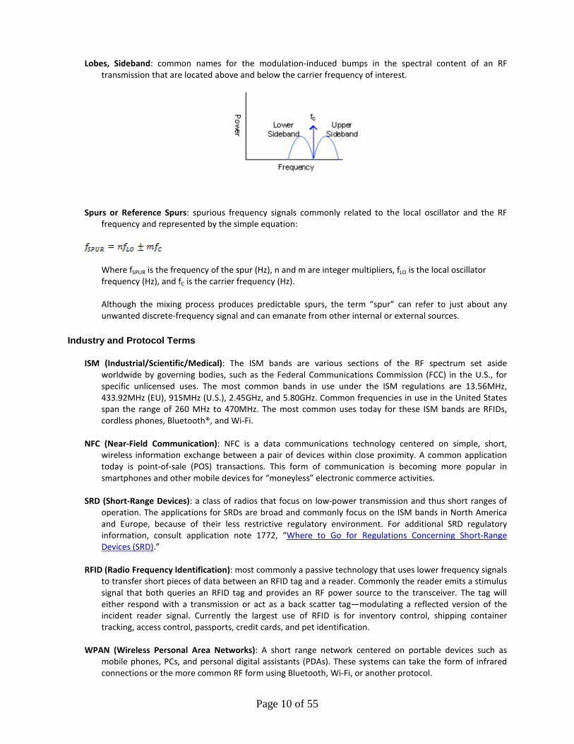
Lobes, Sideband: common names for the modulation-induced bumps in the spectral content of an RF transmission that are located above and below the carrier frequency of interest.

Spurs or Reference Spurs: spurious frequency signals commonly related to the local oscillator and the RF

frequency and represented by the simple equation:

Where fSPUR is the frequency of the spur (Hz), n and m are integer multipliers, fLO is the local oscillator frequency (Hz), and fC is the carrier frequency (Hz). Although the mixing process produces predictable spurs, the term “spur” can refer to just about any unwanted discrete-frequency signal and can emanate from other internal or external sources.

Industry and Protocol Terms

ISM (Industrial/Scientific/Medical): The ISM bands are various sections of the RF spectrum set aside worldwide by governing bodies, such as the Federal Communications Commission (FCC) in the U.S., for specific unlicensed uses. The most common bands in use under the ISM regulations are 13.56MHz, 433.92MHz (EU), 915MHz (U.S.), 2.45GHz, and 5.80GHz. Common frequencies in use in the United States span the range of 260 MHz to 470MHz. The most common uses today for these ISM bands are RFIDs, cordless phones, Bluetooth®, and Wi-Fi.

NFC (Near-Field Communication): NFC is a data communications technology centered on simple, short,

wireless information exchange between a pair of devices within close proximity. A common application today is point-of-sale (POS) transactions. This form of communication is becoming more popular in smartphones and other mobile devices for “moneyless” electronic commerce activities.

SRD (Short-Range Devices): a class of radios that focus on low-power transmission and thus short ranges of

operation. The applications for SRDs are broad and commonly focus on the ISM bands in North America and Europe, because of their less restrictive regulatory environment. For additional SRD regulatory information, consult application note 1772, “Where to Go for Regulations Concerning Short-Range Devices (SRD).”

RFID (Radio Frequency Identification): most commonly a passive technology that uses lower frequency signals

to transfer short pieces of data between an RFID tag and a reader. Commonly the reader emits a stimulus signal that both queries an RFID tag and provides an RF power source to the transceiver. The tag will either respond with a transmission or act as a back scatter tag—modulating a reflected version of the incident reader signal. Currently the largest use of RFID is for inventory control, shipping container tracking, access control, passports, credit cards, and pet identification.

WPAN (Wireless Personal Area Networks): A short range network centered on portable devices such as

mobile phones, PCs, and personal digital assistants (PDAs). These systems can take the form of infrared connections or the more common RF form using Bluetooth, Wi-Fi, or another protocol.

Page 11 of 55

Encoding: describes a method of turning raw digital data (0s and 1s) into a formatted signal used to modulate the carrier for transmission. Techniques for encoding data are many and varied. Encoding can simply be a definition of which bits in a serial stream of data represents what information (address, data, etc.) or as complex as the schemes noted in the following text.

RZ (Return to Zero), NRZ (Nonreturn to Zero): descriptive methods of encoding data for transmission in an RF

system. A common baseband decoding method that uses a data slicer requires that an average level be generated to compare against an analog signal, and thus determine a data bit stream. If an NRZ system is used to encode data, then there is a possibility that a long string of 0s or 1s will adversely affect the average level and thus cause duty cycle or even decoding errors.

Manchester Encoding: a method of edge encoding data

in an RZ fashion such that the baseband data signal does not remain fixed at one logic level for an extended time. (refer to application note 3435, “Manchester Data Encoding for Radio Communications”). This method of encoding doubles the bandwidth required for a given data rate. As an example, an NRZ data rate of 1kbps (native 0101… string is a 1kHz square wave) when Manchester encoded would result in an effective 2kHz square wave (if encoding a 0000… or 1111… string).

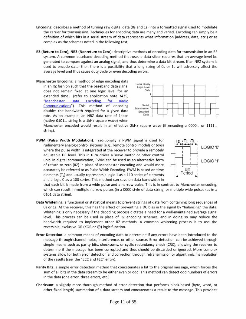
PWM (Pulse Width Modulation): Traditionally a PWM signal is used for

rudimentary analog-control systems (e.g., remote control models or toys) where the pulse width is integrated at the receiver to provide a remotely adjustable DC level. This in turn drives a servo motor or other control unit. In digital communication, PWM can be used as an alternative form of return to zero (RZ) in place of Manchester encoding and would more accurately be referred to as Pulse Width Encoding. PWM is based on time elements (TE) and usually represents a logic 1 as a 110 series of elements and a logic 0 as a 100 series. This method can save on data bandwidth in that each bit is made from a wide pulse and a narrow pulse. This is in contrast to Manchester encoding, which can result in multiple narrow pulses (in a 0000 style of data string) or multiple wide pulses (as in a 0101 data string).

Data Whitening: a functional or statistical means to prevent strings of data from containing long sequences of 0s or 1s. At the receiver, this has the effect of preventing a DC bias in the signal by “balancing” the data. Whitening is only necessary if the decoding process dictates a need for a well-maintained average signal level. This process can be used in place of RZ encoding schemes, and in doing so may reduce the bandwidth required to implement other RZ methods. A common whitening process is to use the reversible, exclusive-OR (XOR or ) logic function.

Error Detection: a common means of encoding data to determine if any errors have been introduced to the message through channel noise, interference, or other source. Error detection can be achieved through simple means such as parity bits, checksums, or cyclic redundancy check (CRC), allowing the receiver to determine if the message has been corrupted and thus should be discarded or ignored. More complex systems allow for both error detection and correction through retransmission or algorithmic manipulation of the results (see the "ECC and FEC” entry).

Parity Bits: a simple error detection method that concatenates a bit to the original message, which forces the sum of all bits in the data stream to be either even or odd. This method can detect odd numbers of errors in the data (one error, three errors, etc.).

Checksum: a slightly more thorough method of error detection that performs block-based (byte, word, or other fixed length) summation of a data stream and concatenates a result to the message. This provides

Page 12 of 55

the next level of detection beyond parity by forcing higher error rates before the system breaks down and cannot identify the occurrence of corruption.

Cyclic Redundancy Check (CRC): a sophisticated, common, and robust form of error detection used in today’s wired and wireless systems. CRC uses a polynomial code for hashing a checksum out of a block of data and is designed to detect accidental changes in the raw payload. Its functions are commonly implemented in hardware to speed up the process of calculating the outgoing CRC and for quickly confirming the validity of a received CRC.

ECC (Error Correction Code) and FEC (Forward Error Correction), Hamming Code: a method of adding redundant information to a data stream that allows for identification and correction of errors, and thus reduces or eliminates the need for retransmission. There are two main types of FEC methods: fixed-length block coding and variable-length convolutional coding. FEC is implemented in both the transmitter to encode the data, and the receiver to recover lost data from a noisy communication channel.

Encryption: a method of applying a cipher (algorithm) to information in order to intentionally obscure the content and to make it unintelligible for those not authorized to view or receive the information.

AES128 (Advanced Encryption Standard – 128-bit): A standardized form of symmetric key encryption using a 128-bit block cipher (also with 192-bit and 256-bit versions) to encrypt and decrypt data. AES has been approved for use by the U.S. Department of Defense.

Instruments

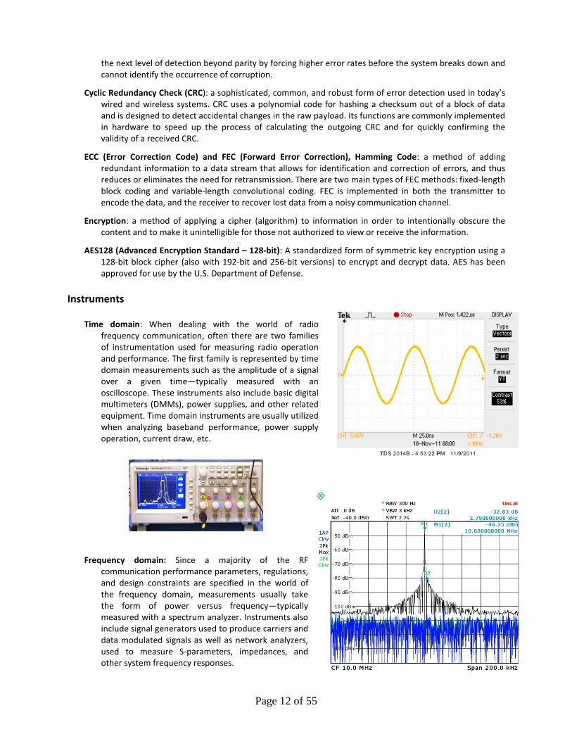
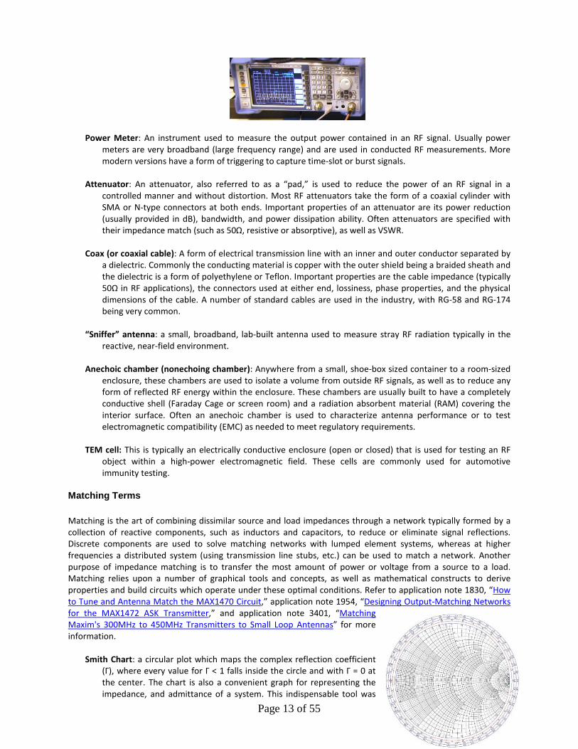
Time domain: When dealing with the world of radio frequency communication, often there are two families of instrumentation used for measuring radio operation and performance. The first family is represented by time domain measurements such as the amplitude of a signal over a given time—typically measured with an oscilloscope. These instruments also include basic digital multimeters (DMMs), power supplies, and other related equipment. Time domain instruments are usually utilized when analyzing baseband performance, power supply operation, current draw, etc.

Frequency domain: Since a majority of the RF

communication performance parameters, regulations, and design constraints are specified in the world of the frequency domain, measurements usually take the form of power versus frequency—typically measured with a spectrum analyzer. Instruments also include signal generators used to produce carriers and data modulated signals as well as network analyzers, used to measure S-parameters, impedances, and other system frequency responses.

Page 13 of 55

Power Meter: An instrument used to measure the output power contained in an RF signal. Usually power

meters are very broadband (large frequency range) and are used in conducted RF measurements. More modern versions have a form of triggering to capture time-slot or burst signals.

Attenuator: An attenuator, also referred to as a “pad,” is used to reduce the power of an RF signal in a

controlled manner and without distortion. Most RF attenuators take the form of a coaxial cylinder with SMA or N-type connectors at both ends. Important properties of an attenuator are its power reduction (usually provided in dB), bandwidth, and power dissipation ability. Often attenuators are specified with their impedance match (such as 50Ω, resistive or absorptive), as well as VSWR.

Coax (or coaxial cable): A form of electrical transmission line with an inner and outer conductor separated by

a dielectric. Commonly the conducting material is copper with the outer shield being a braided sheath and the dielectric is a form of polyethylene or Teflon. Important properties are the cable impedance (typically 50Ω in RF applications), the connectors used at either end, lossiness, phase properties, and the physical dimensions of the cable. A number of standard cables are used in the industry, with RG-58 and RG-174 being very common.

“Sniffer” antenna: a small, broadband, lab-built antenna used to measure stray RF radiation typically in the

reactive, near-field environment. Anechoic chamber (nonechoing chamber): Anywhere from a small, shoe-box sized container to a room-sized

enclosure, these chambers are used to isolate a volume from outside RF signals, as well as to reduce any form of reflected RF energy within the enclosure. These chambers are usually built to have a completely conductive shell (Faraday Cage or screen room) and a radiation absorbent material (RAM) covering the interior surface. Often an anechoic chamber is used to characterize antenna performance or to test electromagnetic compatibility (EMC) as needed to meet regulatory requirements.

TEM cell: This is typically an electrically conductive enclosure (open or closed) that is used for testing an RF

object within a high-power electromagnetic field. These cells are commonly used for automotive immunity testing.

Matching Terms Matching is the art of combining dissimilar source and load impedances through a network typically formed by a collection of reactive components, such as inductors and capacitors, to reduce or eliminate signal reflections. Discrete components are used to solve matching networks with lumped element systems, whereas at higher frequencies a distributed system (using transmission line stubs, etc.) can be used to match a network. Another purpose of impedance matching is to transfer the most amount of power or voltage from a source to a load. Matching relies upon a number of graphical tools and concepts, as well as mathematical constructs to derive properties and build circuits which operate under these optimal conditions. Refer to application note 1830, “How to Tune and Antenna Match the MAX1470 Circuit,” application note 1954, “Designing Output-Matching Networks for the MAX1472 ASK Transmitter,” and application note 3401, “Matching Maxim's 300MHz to 450MHz Transmitters to Small Loop Antennas” for more information.

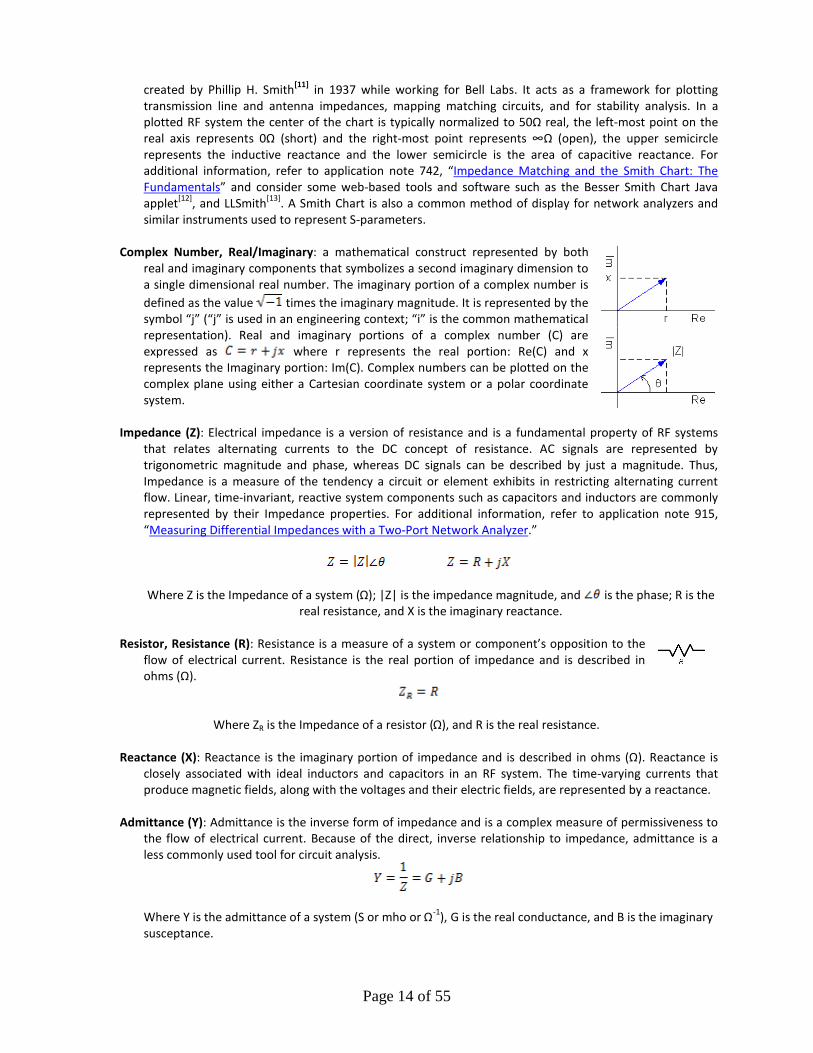
Smith Chart: a circular plot which maps the complex reflection coefficient

(Γ), where every value for Γ < 1 falls inside the circle and with Γ = 0 at the center. The chart is also a convenient graph for representing the impedance, and admittance of a system. This indispensable tool was

Page 14 of 55

created by Phillip H. Smith[11] in 1937 while working for Bell Labs. It acts as a framework for plotting transmission line and antenna impedances, mapping matching circuits, and for stability analysis. In a plotted RF system the center of the chart is typically normalized to 50Ω real, the left-most point on the real axis represents 0Ω (short) and the right-most point represents ∞Ω (open), the upper semicircle represents the inductive reactance and the lower semicircle is the area of capacitive reactance. For additional information, refer to application note 742, “Impedance Matching and the Smith Chart: The Fundamentals” and consider some web-based tools and software such as the Besser Smith Chart Java applet[12], and LLSmith[13]. A Smith Chart is also a common method of display for network analyzers and similar instruments used to represent S-parameters.

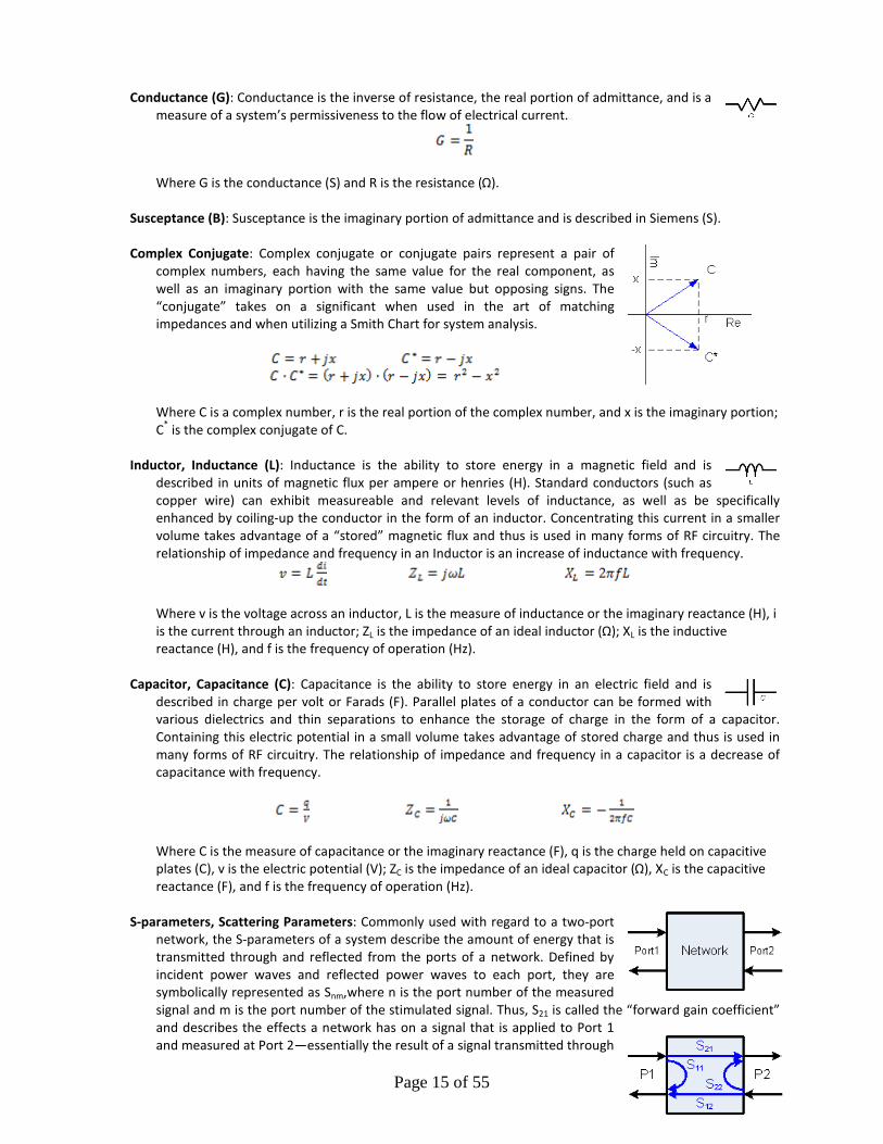
Complex Number, Real/Imaginary: a mathematical construct represented by both

real and imaginary components that symbolizes a second imaginary dimension to a single dimensional real number. The imaginary portion of a complex number is defined as the value times the imaginary magnitude. It is represented by the symbol “j” (“j” is used in an engineering context; “i” is the common mathematical representation). Real and imaginary portions of a complex number (C) are expressed as where r represents the real portion: Re(C) and x represents the Imaginary portion: Im(C). Complex numbers can be plotted on the complex plane using either a Cartesian coordinate system or a polar coordinate system.

Impedance (Z): Electrical impedance is a version of resistance and is a fundamental property of RF systems

that relates alternating currents to the DC concept of resistance. AC signals are represented by trigonometric magnitude and phase, whereas DC signals can be described by just a magnitude. Thus, Impedance is a measure of the tendency a circuit or element exhibits in restricting alternating current flow. Linear, time-invariant, reactive system components such as capacitors and inductors are commonly represented by their Impedance properties. For additional information, refer to application note 915, “Measuring Differential Impedances with a Two-Port Network Analyzer.”

Where Z is the Impedance of a system (Ω); |Z| is the impedance magnitude, and is the phase; R is the

real resistance, and X is the imaginary reactance. Resistor, Resistance (R): Resistance is a measure of a system or component’s opposition to the

flow of electrical current. Resistance is the real portion of impedance and is described in ohms (Ω).

Where ZR is the Impedance of a resistor (Ω), and R is the real resistance.

Reactance (X): Reactance is the imaginary portion of impedance and is described in ohms (Ω). Reactance is closely associated with ideal inductors and capacitors in an RF system. The time-varying currents that produce magnetic fields, along with the voltages and their electric fields, are represented by a reactance.

Admittance (Y): Admittance is the inverse form of impedance and is a complex measure of permissiveness to

the flow of electrical current. Because of the direct, inverse relationship to impedance, admittance is a less commonly used tool for circuit analysis.

Where Y is the admittance of a system (S or mho or Ω-1), G is the real conductance, and B is the imaginary susceptance.

Page 15 of 55

Conductance (G): Conductance is the inverse of resistance, the real portion of admittance, and is a measure of a system’s permissiveness to the flow of electrical current.

Where G is the conductance (S) and R is the resistance (Ω). Susceptance (B): Susceptance is the imaginary portion of admittance and is described in Siemens (S). Complex Conjugate: Complex conjugate or conjugate pairs represent a pair of

complex numbers, each having the same value for the real component, as well as an imaginary portion with the same value but opposing signs. The “conjugate” takes on a significant when used in the art of matching impedances and when utilizing a Smith Chart for system analysis.

Where C is a complex number, r is the real portion of the complex number, and x is the imaginary portion; C* is the complex conjugate of C.

Inductor, Inductance (L): Inductance is the ability to store energy in a magnetic field and is

described in units of magnetic flux per ampere or henries (H). Standard conductors (such as copper wire) can exhibit measureable and relevant levels of inductance, as well as be specifically enhanced by coiling-up the conductor in the form of an inductor. Concentrating this current in a smaller volume takes advantage of a “stored” magnetic flux and thus is used in many forms of RF circuitry. The relationship of impedance and frequency in an Inductor is an increase of inductance with frequency.

Where v is the voltage across an inductor, L is the measure of inductance or the imaginary reactance (H), i is the current through an inductor; ZL is the impedance of an ideal inductor (Ω); XL is the inductive reactance (H), and f is the frequency of operation (Hz).

Capacitor, Capacitance (C): Capacitance is the ability to store energy in an electric field and is

described in charge per volt or Farads (F). Parallel plates of a conductor can be formed with various dielectrics and thin separations to enhance the storage of charge in the form of a capacitor. Containing this electric potential in a small volume takes advantage of stored charge and thus is used in many forms of RF circuitry. The relationship of impedance and frequency in a capacitor is a decrease of capacitance with frequency.

Where C is the measure of capacitance or the imaginary reactance (F), q is the charge held on capacitive plates (C), v is the electric potential (V); ZC is the impedance of an ideal capacitor (Ω), XC is the capacitive reactance (F), and f is the frequency of operation (Hz).

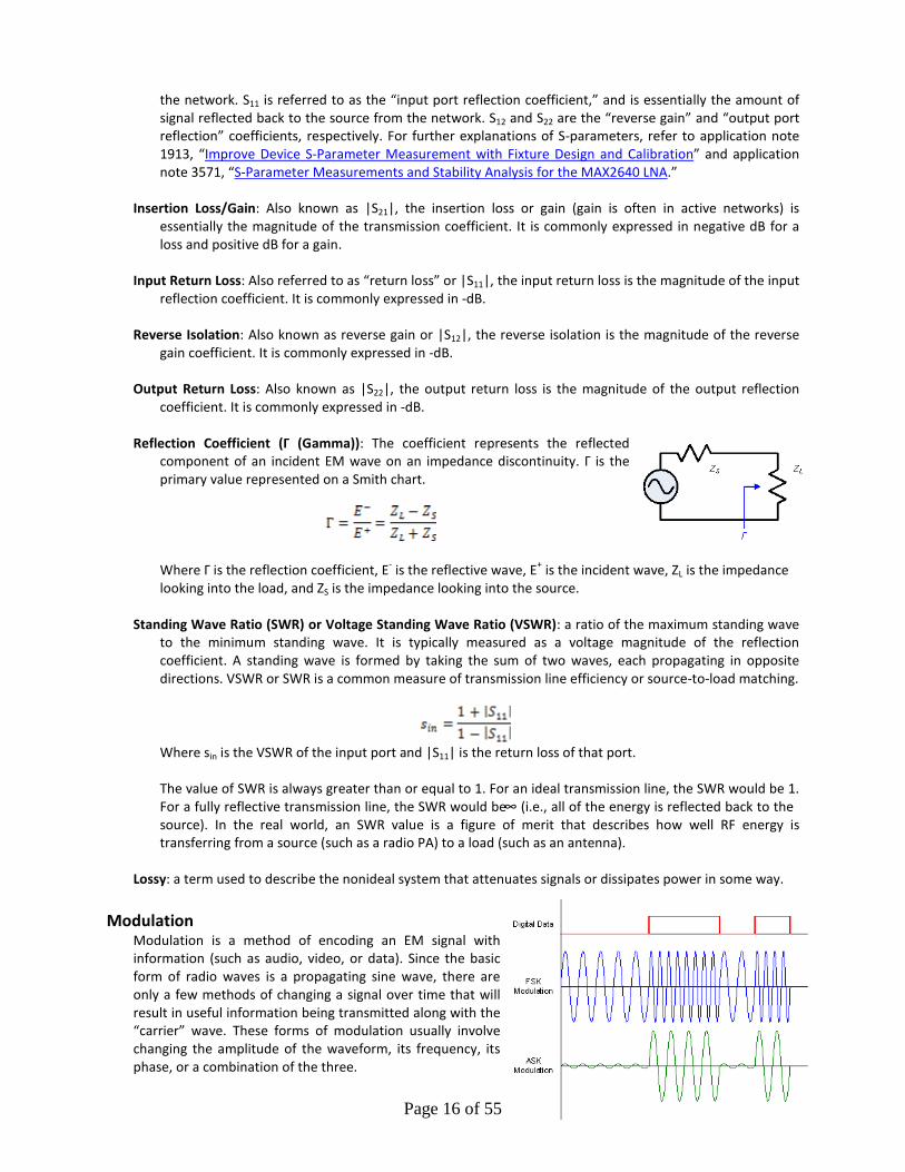
S-parameters, Scattering Parameters: Commonly used with regard to a two-port

network, the S-parameters of a system describe the amount of energy that is transmitted through and reflected from the ports of a network. Defined by incident power waves and reflected power waves to each port, they are symbolically represented as Snm,where n is the port number of the measured signal and m is the port number of the stimulated signal. Thus, S21 is called the “forward gain coefficient” and describes the effects a network has on a signal that is applied to Port 1 and measured at Port 2—essentially the result of a signal transmitted through

Page 16 of 55

the network. S11 is referred to as the “input port reflection coefficient,” and is essentially the amount of signal reflected back to the source from the network. S12 and S22 are the “reverse gain” and “output port reflection” coefficients, respectively. For further explanations of S-parameters, refer to application note 1913, “Improve Device S-Parameter Measurement with Fixture Design and Calibration” and application note 3571, “S-Parameter Measurements and Stability Analysis for the MAX2640 LNA.”

Insertion Loss/Gain: Also known as |S21|, the insertion loss or gain (gain is often in active networks) is

essentially the magnitude of the transmission coefficient. It is commonly expressed in negative dB for a loss and positive dB for a gain.

Input Return Loss: Also referred to as “return loss” or |S11|, the input return loss is the magnitude of the input

reflection coefficient. It is commonly expressed in -dB. Reverse Isolation: Also known as reverse gain or |S12|, the reverse isolation is the magnitude of the reverse

gain coefficient. It is commonly expressed in -dB. Output Return Loss: Also known as |S22|, the output return loss is the magnitude of the output reflection

coefficient. It is commonly expressed in -dB. Reflection Coefficient (Γ (Gamma)): The coefficient represents the reflected

component of an incident EM wave on an impedance discontinuity. Γ is the primary value represented on a Smith chart.

Where Γ is the reflection coefficient, E- is the reflective wave, E+ is the incident wave, ZL is the impedance looking into the load, and ZS is the impedance looking into the source.

Standing Wave Ratio (SWR) or Voltage Standing Wave Ratio (VSWR): a ratio of the maximum standing wave

to the minimum standing wave. It is typically measured as a voltage magnitude of the reflection coefficient. A standing wave is formed by taking the sum of two waves, each propagating in opposite directions. VSWR or SWR is a common measure of transmission line efficiency or source-to-load matching.

Where sin is the VSWR of the input port and |S11| is the return loss of that port. The value of SWR is always greater than or equal to 1. For an ideal transmission line, the SWR would be 1. For a fully reflective transmission line, the SWR would be ∞ (i.e., all of the energy is reflected back to the source). In the real world, an SWR value is a figure of merit that describes how well RF energy is transferring from a source (such as a radio PA) to a load (such as an antenna).

Lossy: a term used to describe the nonideal system that attenuates signals or dissipates power in some way.

Modulation

Modulation is a method of encoding an EM signal with information (such as audio, video, or data). Since the basic form of radio waves is a propagating sine wave, there are only a few methods of changing a signal over time that will result in useful information being transmitted along with the “carrier” wave. These forms of modulation usually involve changing the amplitude of the waveform, its frequency, its phase, or a combination of the three.

Page 17 of 55

Data rate: the frequency of digital content being encoded and used to modulate the carrier signal. Often listed with units of bits per second (bps) or occasionally as Hz (such as when using a square wave for diagnostic purposes).

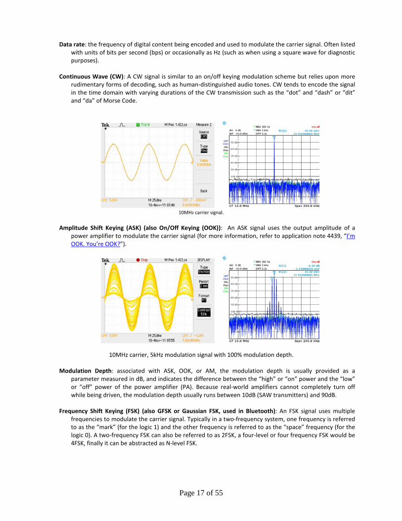
Continuous Wave (CW): A CW signal is similar to an on/off keying modulation scheme but relies upon more

rudimentary forms of decoding, such as human-distinguished audio tones. CW tends to encode the signal in the time domain with varying durations of the CW transmission such as the “dot” and “dash” or “dit” and “da” of Morse Code.

10MHz carrier signal.

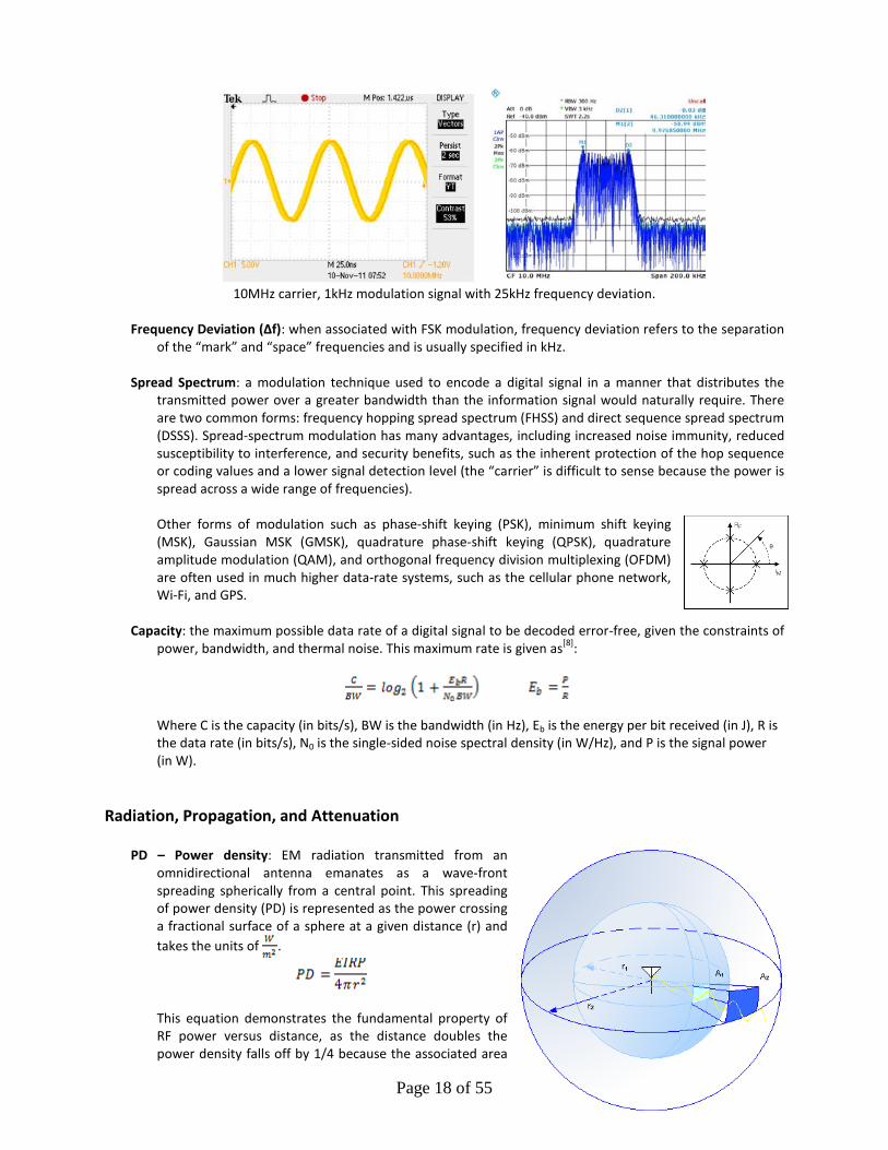
Amplitude Shift Keying (ASK) (also On/Off Keying (OOK)): An ASK signal uses the output amplitude of a

power amplifier to modulate the carrier signal (for more information, refer to application note 4439, “I’m OOK. You’re OOK?”).

10MHz carrier, 5kHz modulation signal with 100% modulation depth. Modulation Depth: associated with ASK, OOK, or AM, the modulation depth is usually provided as a

parameter measured in dB, and indicates the difference between the “high” or “on” power and the “low” or “off” power of the power amplifier (PA). Because real-world amplifiers cannot completely turn off while being driven, the modulation depth usually runs between 10dB (SAW transmitters) and 90dB.

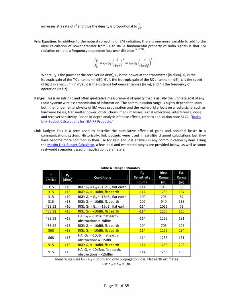
Frequency Shift Keying (FSK) (also GFSK or Gaussian FSK, used in Bluetooth): An FSK signal uses multiple

frequencies to modulate the carrier signal. Typically in a two-frequency system, one frequency is referred to as the “mark” (for the logic 1) and the other frequency is referred to as the “space” frequency (for the logic 0). A two-frequency FSK can also be referred to as 2FSK, a four-level or four frequency FSK would be 4FSK, finally it can be abstracted as N-level FSK.

Page 18 of 55

10MHz carrier, 1kHz modulation signal with 25kHz frequency deviation.

Frequency Deviation (Δf): when associated with FSK modulation, frequency deviation refers to the separation

of the “mark” and “space” frequencies and is usually specified in kHz. Spread Spectrum: a modulation technique used to encode a digital signal in a manner that distributes the

transmitted power over a greater bandwidth than the information signal would naturally require. There are two common forms: frequency hopping spread spectrum (FHSS) and direct sequence spread spectrum (DSSS). Spread-spectrum modulation has many advantages, including increased noise immunity, reduced susceptibility to interference, and security benefits, such as the inherent protection of the hop sequence or coding values and a lower signal detection level (the “carrier” is difficult to sense because the power is spread across a wide range of frequencies).

Other forms of modulation such as phase-shift keying (PSK), minimum shift keying (MSK), Gaussian MSK (GMSK), quadrature phase-shift keying (QPSK), quadrature amplitude modulation (QAM), and orthogonal frequency division multiplexing (OFDM) are often used in much higher data-rate systems, such as the cellular phone network, Wi-Fi, and GPS.

Capacity: the maximum possible data rate of a digital signal to be decoded error-free, given the constraints of

power, bandwidth, and thermal noise. This maximum rate is given as[8]:

Where C is the capacity (in bits/s), BW is the bandwidth (in Hz), Eb is the energy per bit received (in J), R is the data rate (in bits/s), N0 is the single-sided noise spectral density (in W/Hz), and P is the signal power (in W).

Radiation, Propagation, and Attenuation

PD – Power density: EM radiation transmitted from an omnidirectional antenna emanates as a wave-front spreading spherically from a central point. This spreading of power density (PD) is represented as the power crossing a fractional surface of a sphere at a given distance (r) and takes the units of .

This equation demonstrates the fundamental property of RF power versus distance, as the distance doubles the power density falls off by 1/4 because the associated area

Page 19 of 55

increases at a rate of r2 and thus the density is proportional to .

Friis Equation: In addition to the natural spreading of EM radiation, there is one more variable to add to the ideal calculation of power transfer from TX to RX. A fundamental property of radio signals is that EM radiation exhibits a frequency-dependent loss over distance [6, p774].

Where PR is the power at the receiver (in dBm), PT is the power at the transmitter (in dBm), GT is the isotropic gain of the TX antenna (in dBi), GR is the isotropic gain of the RX antenna (in dBi), c is the speed of light in a vacuum (in m/s), d is the distance between antennas (in m), and f is the frequency of operation (in Hz).

Range: This is an intrinsic and often qualitative measurement of quality that is usually the ultimate goal of any

radio system: wireless transmission of information. The communication range is highly dependent upon both the fundamental physics of EM wave propagation and the real-world effects on a radio signal such as hardware losses, transmitter power, obstructions, medium losses, signal reflections, interference, noise, and receiver sensitivity. For an in-depth analysis of these effects, refer to application note 5142, “Radio Link-Budget Calculations for ISM-RF Products.”

Link Budget: This is a term used to describe the cumulative effects of gains and nonideal losses in a

communications system. Historically, link budgets were used in satellite channel calculations but they have become more common in their use for gain and loss analysis in any communication system. Using the Maxim Link-Budget Calculator, a few ideal and estimated ranges are provided below, as well as some real-world scenarios based on application parameters.

Table 4. Range Estimates

f (MHz)

PT (dBm) Conditions

PR Sensitivity

Ideal Range

Est. Range

(dBm) (m) (m) 315 +10 RKE: GT = GR = -15dBi, flat earth -114 1055 69 315 +13 RKE: GT = -10dBi, flat earth -114 1255 167 315 +10 RKE: GT = GR = -15dBi, flat earth -109 795 57 315 +13 RKE: GT = -10dBi, flat earth -109 940 138

433.92 +10 RKE: GT = GR = -15dBi, flat earth -114 1055 76 433.92 +13 RKE: GT = -10dBi, flat earth -114 1255 185

433.92 +13 HA: GT = -10dBi, flat earth, obstructions = -9dBm -114 1255 131

433.92 +13 RKE: GT = -10dBi, flat earth -104 705 126 868 +13 RKE: GT = -10dBi, flat earth -114 1255 234

868 +13 HA: GT = -10dBi, flat earth, obstructions = -15dBi -114 1255 131

915 +13 RKE: GT = -10dBi, flat earth -114 1255 238

915 +13 HA: GT = -10dBm, flat earth, obstructions = -15dBm -114 1255 133

Ideal range uses GT = GR = 0dBm and only propagation loss. Flat earth estimates use hTX = hRX = 1m.

Page 20 of 55

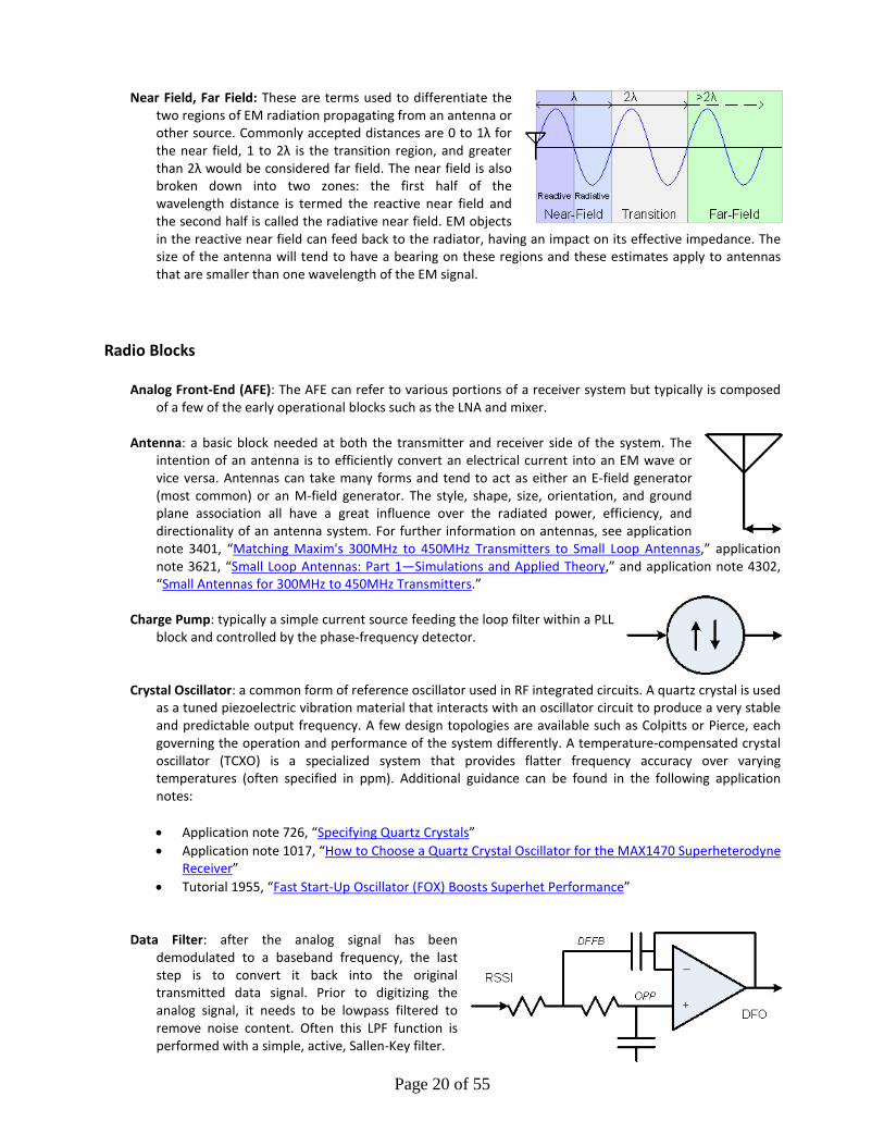
Near Field, Far Field: These are terms used to differentiate the two regions of EM radiation propagating from an antenna or other source. Commonly accepted distances are 0 to 1λ for the near field, 1 to 2λ is the transition region, and greater than 2λ would be considered far field. The near field is also broken down into two zones: the first half of the wavelength distance is termed the reactive near field and the second half is called the radiative near field. EM objects in the reactive near field can feed back to the radiator, having an impact on its effective impedance. The size of the antenna will tend to have a bearing on these regions and these estimates apply to antennas that are smaller than one wavelength of the EM signal.

Radio Blocks

Analog Front-End (AFE): The AFE can refer to various portions of a receiver system but typically is composed of a few of the early operational blocks such as the LNA and mixer.

Antenna: a basic block needed at both the transmitter and receiver side of the system. The

intention of an antenna is to efficiently convert an electrical current into an EM wave or vice versa. Antennas can take many forms and tend to act as either an E-field generator (most common) or an M-field generator. The style, shape, size, orientation, and ground plane association all have a great influence over the radiated power, efficiency, and directionality of an antenna system. For further information on antennas, see application note 3401, “Matching Maxim's 300MHz to 450MHz Transmitters to Small Loop Antennas,” application note 3621, “Small Loop Antennas: Part 1—Simulations and Applied Theory,” and application note 4302, “Small Antennas for 300MHz to 450MHz Transmitters.”

Charge Pump: typically a simple current source feeding the loop filter within a PLL

block and controlled by the phase-frequency detector. Crystal Oscillator: a common form of reference oscillator used in RF integrated circuits. A quartz crystal is used

as a tuned piezoelectric vibration material that interacts with an oscillator circuit to produce a very stable and predictable output frequency. A few design topologies are available such as Colpitts or Pierce, each governing the operation and performance of the system differently. A temperature-compensated crystal oscillator (TCXO) is a specialized system that provides flatter frequency accuracy over varying temperatures (often specified in ppm). Additional guidance can be found in the following application notes:

• Application note 726, “Specifying Quartz Crystals” • Application note 1017, “How to Choose a Quartz Crystal Oscillator for the MAX1470 Superheterodyne

Receiver” • Tutorial 1955, “Fast Start-Up Oscillator (FOX) Boosts Superhet Performance”

Data Filter: after the analog signal has been

demodulated to a baseband frequency, the last step is to convert it back into the original transmitted data signal. Prior to digitizing the analog signal, it needs to be lowpass filtered to remove noise content. Often this LPF function is performed with a simple, active, Sallen-Key filter.

Page 21 of 55

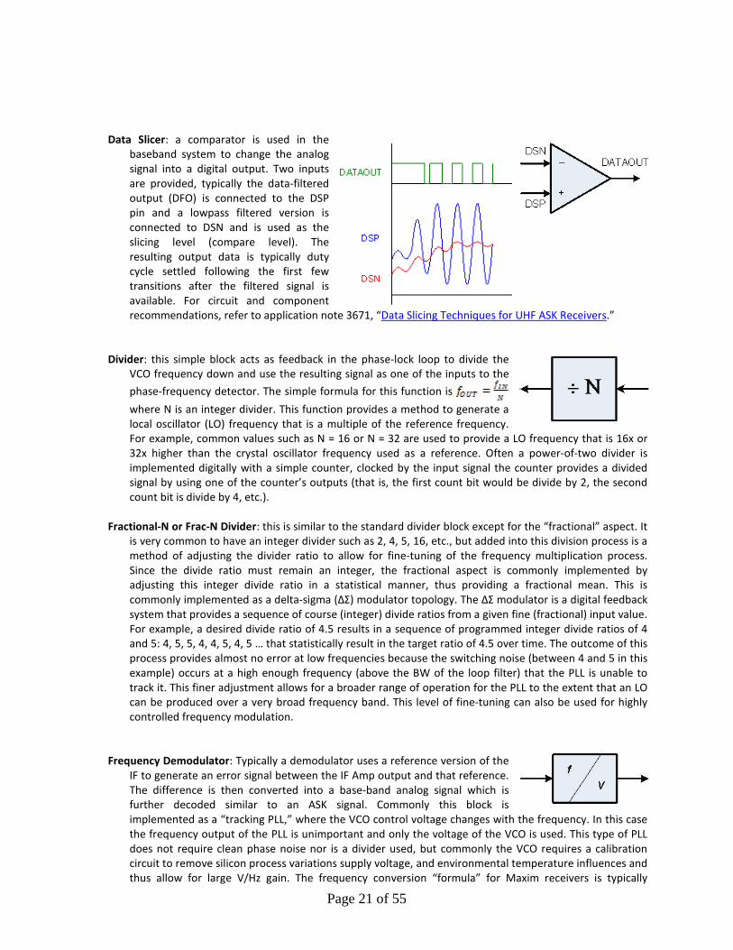
Data Slicer: a comparator is used in the

baseband system to change the analog signal into a digital output. Two inputs are provided, typically the data-filtered output (DFO) is connected to the DSP pin and a lowpass filtered version is connected to DSN and is used as the slicing level (compare level). The resulting output data is typically duty cycle settled following the first few transitions after the filtered signal is available. For circuit and component recommendations, refer to application note 3671, “Data Slicing Techniques for UHF ASK Receivers.”

Divider: this simple block acts as feedback in the phase-lock loop to divide the

VCO frequency down and use the resulting signal as one of the inputs to the phase-frequency detector. The simple formula for this function is where N is an integer divider. This function provides a method to generate a local oscillator (LO) frequency that is a multiple of the reference frequency. For example, common values such as N = 16 or N = 32 are used to provide a LO frequency that is 16x or 32x higher than the crystal oscillator frequency used as a reference. Often a power-of-two divider is implemented digitally with a simple counter, clocked by the input signal the counter provides a divided signal by using one of the counter’s outputs (that is, the first count bit would be divide by 2, the second count bit is divide by 4, etc.).

Fractional-N or Frac-N Divider: this is similar to the standard divider block except for the “fractional” aspect. It

is very common to have an integer divider such as 2, 4, 5, 16, etc., but added into this division process is a method of adjusting the divider ratio to allow for fine-tuning of the frequency multiplication process. Since the divide ratio must remain an integer, the fractional aspect is commonly implemented by adjusting this integer divide ratio in a statistical manner, thus providing a fractional mean. This is commonly implemented as a delta-sigma (ΔΣ) modulator topology. The ΔΣ modulator is a digital feedback system that provides a sequence of course (integer) divide ratios from a given fine (fractional) input value. For example, a desired divide ratio of 4.5 results in a sequence of programmed integer divide ratios of 4 and 5: 4, 5, 5, 4, 4, 5, 4, 5 … that statistically result in the target ratio of 4.5 over time. The outcome of this process provides almost no error at low frequencies because the switching noise (between 4 and 5 in this example) occurs at a high enough frequency (above the BW of the loop filter) that the PLL is unable to track it. This finer adjustment allows for a broader range of operation for the PLL to the extent that an LO can be produced over a very broad frequency band. This level of fine-tuning can also be used for highly controlled frequency modulation.

Frequency Demodulator: Typically a demodulator uses a reference version of the

IF to generate an error signal between the IF Amp output and that reference. The difference is then converted into a base-band analog signal which is further decoded similar to an ASK signal. Commonly this block is implemented as a “tracking PLL,” where the VCO control voltage changes with the frequency. In this case the frequency output of the PLL is unimportant and only the voltage of the VCO is used. This type of PLL does not require clean phase noise nor is a divider used, but commonly the VCO requires a calibration circuit to remove silicon process variations supply voltage, and environmental temperature influences and thus allow for large V/Hz gain. The frequency conversion “formula” for Maxim receivers is typically

Page 22 of 55

between 2.0 and 2.2mV/kHz. An older version of the frequency demodulator was call a discriminator and functioned by detecting a frequency-dependent imbalance in a transformer.

Image Rejection Mixer: an IR mixer uses an in-phase quadrature (IQ) local

oscillator (LO) and two mixing cells, resulting in two signal outputs that are shifted 90° in phase. A signal that is mixed above the LO will result in a phase shift in one direction at IF and a signal mixed below the LO will show a phase shift in the other direction. The IR mixer is essentially an all-pass network with unity amplitude that provides a phase shift to the heterodyned signals. By summing the two IF signals back together, one mixed frequency (fC) will be trigonometrically summed resulting in a signal gain (of about 6dB), and the other mixed frequency (fIM) will be subtracted resulting in a signal attenuation (of around 30dB, possibly as high as 40dB).

Intermediate Frequency (IF) Amplifier: often referred to as the “RSSI amp” or “IF

limiting amp.” This block is a chain of amplifiers that successively amplify and limit the IF signal, producing one output that only varies in phase/frequency, and a second output that sums the currents of each gain stage, providing a logarithmic signal strength indication of the received signal’s power. For FSK systems, the output signal of the limiting amplifiers is typically fed to a frequency demodulator and subsequently the signal is used for baseband decoding. In ASK systems the logarithmic summed current from the limiting amplifier stages is used for an RSSI signal or simply a fluctuation in amplitude of the RF signal. In direct-to-digital designs the IF Amp is implemented as a purely linear Variable Gain Amplifier (VGA), with an automatic gain control (AGC) to set the amplitude at the sweet spot of an analog-to-digital converter (ADC).

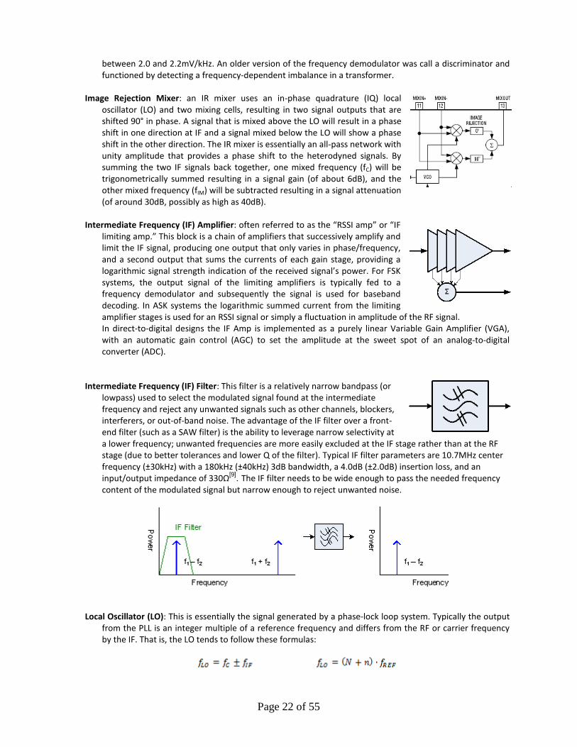
Intermediate Frequency (IF) Filter: This filter is a relatively narrow bandpass (or

lowpass) used to select the modulated signal found at the intermediate frequency and reject any unwanted signals such as other channels, blockers, interferers, or out-of-band noise. The advantage of the IF filter over a front-end filter (such as a SAW filter) is the ability to leverage narrow selectivity at a lower frequency; unwanted frequencies are more easily excluded at the IF stage rather than at the RF stage (due to better tolerances and lower Q of the filter). Typical IF filter parameters are 10.7MHz center frequency (±30kHz) with a 180kHz (±40kHz) 3dB bandwidth, a 4.0dB (±2.0dB) insertion loss, and an input/output impedance of 330Ω[9]. The IF filter needs to be wide enough to pass the needed frequency content of the modulated signal but narrow enough to reject unwanted noise.

Local Oscillator (LO): This is essentially the signal generated by a phase-lock loop system. Typically the output

from the PLL is an integer multiple of a reference frequency and differs from the RF or carrier frequency by the IF. That is, the LO tends to follow these formulas:

Page 23 of 55

Where fLO is the frequency of the local oscillator (Hz), fC is the carrier frequency (Hz), and fIF is the intermediate frequency (Hz). The “±” function depends on whether the IF is a high-side or low-side injection; N is the integer and n is the fraction of the divide ratio, and fREF is the reference oscillator frequency (Hz). The LO is the output from the PLL and as noted in the first formula above, it is used as one of the mixing frequencies along with the RF input signal.

Low-Noise Amplifier (LNA): The LNA is a receiver block operation that gains up

(increases the amplitude of) an input signal with minimal addition of noise. A primary figure of merit for an LNA’s capabilities is its noise figure (NF). By its name, an LNA should provide a large enough gain with a low enough NF so that it can completely dominate the cascaded noise chain of the receiver. The LNA function needs to provide a large enough signal for downstream blocks, so any noise those blocks add to the system does not compromise the final baseband signal.

Loop Filter: a lowpass filter (LPF) used to suppress error signals produced by the

phase-frequency detector and charge pump blocks. Some designs allow control of the feedback system by adjusting the loop filter frequency, bandwidth, settling time, phase margin, etc.

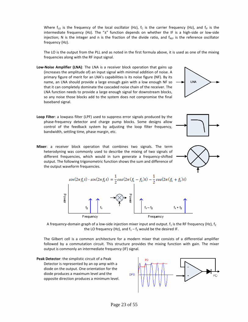
Mixer: a receiver block operation that combines two signals. The term heterodyning was commonly used to describe the mixing of two signals of different frequencies, which would in turn generate a frequency-shifted output. The following trigonometric function shows the sum and difference of the output waveform frequencies.

A frequency-domain graph of a low-side injection mixer input and output. f1 is the RF frequency (Hz), f2

the LO frequency (Hz), and f1 – f2 would be the desired IF. The Gilbert cell is a common architecture for a modern mixer that consists of a differential amplifier followed by a commutation circuit. This structure provides the mixing function with gain. The mixer output is commonly an intermediate frequency (IF) signal.

Peak Detector: the simplistic circuit of a Peak

Detector is represented by an op amp with a diode on the output. One orientation for the diode produces a maximum level and the opposite direction produces a minimum level.

Page 24 of 55

Phase-Frequency Detector (PFD): a phase-frequency detector is used to determine a phase error between two signals. This block will typically provide a command to a charge pump block and a simplistic system can be implemented with an XOR function. Older systems used a simple phase detector, which could accidentally lock onto harmonics or noise. A PFD serves the same function by generating the error signal but does so only within selective frequencies.

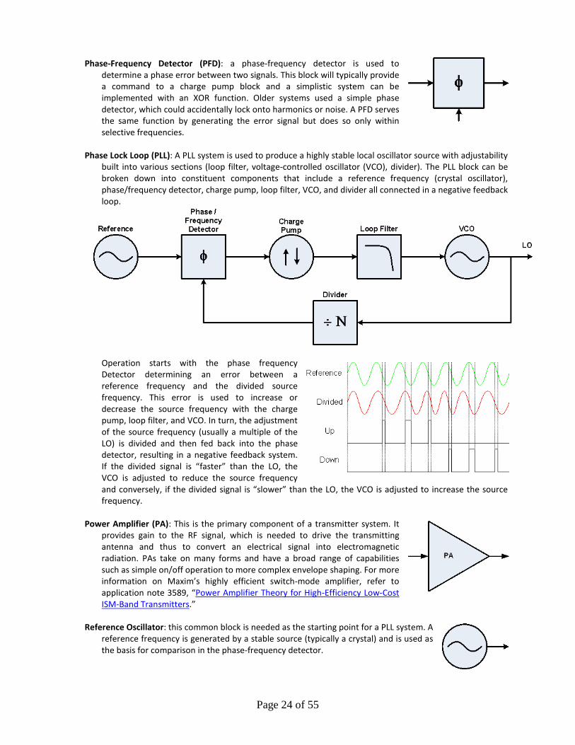
Phase Lock Loop (PLL): A PLL system is used to produce a highly stable local oscillator source with adjustability

built into various sections (loop filter, voltage-controlled oscillator (VCO), divider). The PLL block can be broken down into constituent components that include a reference frequency (crystal oscillator), phase/frequency detector, charge pump, loop filter, VCO, and divider all connected in a negative feedback loop.

Operation starts with the phase frequency Detector determining an error between a reference frequency and the divided source frequency. This error is used to increase or decrease the source frequency with the charge pump, loop filter, and VCO. In turn, the adjustment of the source frequency (usually a multiple of the LO) is divided and then fed back into the phase detector, resulting in a negative feedback system. If the divided signal is “faster” than the LO, the VCO is adjusted to reduce the source frequency and conversely, if the divided signal is “slower” than the LO, the VCO is adjusted to increase the source frequency.

Power Amplifier (PA): This is the primary component of a transmitter system. It

provides gain to the RF signal, which is needed to drive the transmitting antenna and thus to convert an electrical signal into electromagnetic radiation. PAs take on many forms and have a broad range of capabilities such as simple on/off operation to more complex envelope shaping. For more information on Maxim’s highly efficient switch-mode amplifier, refer to application note 3589, “Power Amplifier Theory for High-Efficiency Low-Cost ISM-Band Transmitters.”

Reference Oscillator: this common block is needed as the starting point for a PLL system. A

reference frequency is generated by a stable source (typically a crystal) and is used as the basis for comparison in the phase-frequency detector.

Page 25 of 55

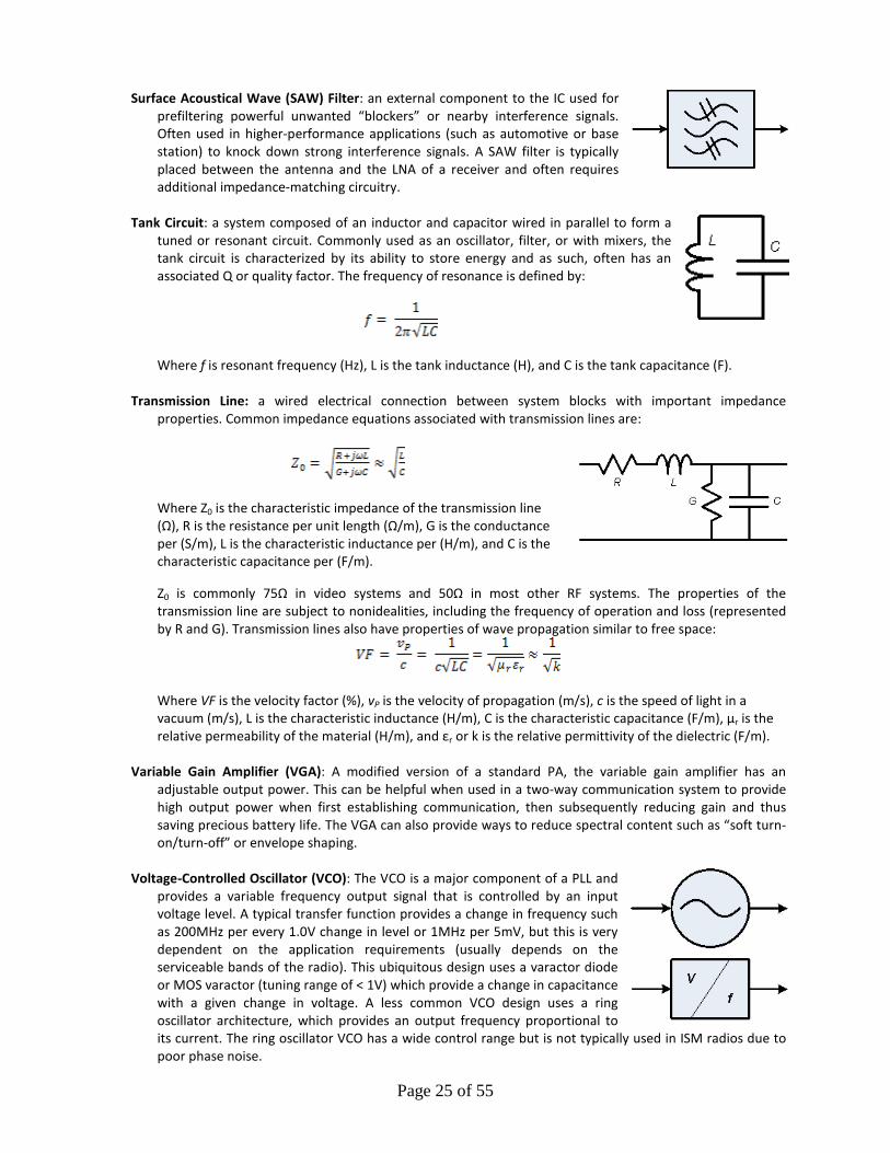
Surface Acoustical Wave (SAW) Filter: an external component to the IC used for prefiltering powerful unwanted “blockers” or nearby interference signals. Often used in higher-performance applications (such as automotive or base station) to knock down strong interference signals. A SAW filter is typically placed between the antenna and the LNA of a receiver and often requires additional impedance-matching circuitry.

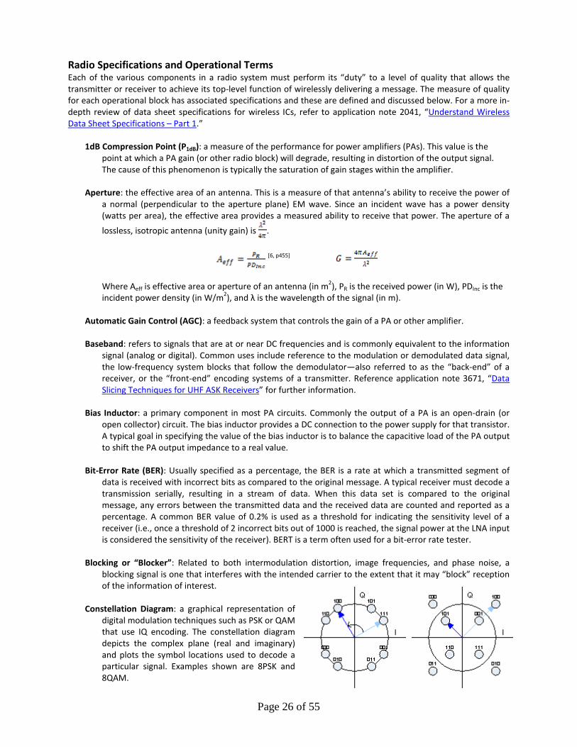
Tank Circuit: a system composed of an inductor and capacitor wired in parallel to form a

tuned or resonant circuit. Commonly used as an oscillator, filter, or with mixers, the tank circuit is characterized by its ability to store energy and as such, often has an associated Q or quality factor. The frequency of resonance is defined by:

Where f is resonant frequency (Hz), L is the tank inductance (H), and C is the tank capacitance (F).

Transmission Line: a wired electrical connection between system blocks with important impedance properties. Common impedance equations associated with transmission lines are:

Where Z0 is the characteristic impedance of the transmission line (Ω), R is the resistance per unit length (Ω/m), G is the conductance per (S/m), L is the characteristic inductance per (H/m), and C is the characteristic capacitance per (F/m).

Z0 is commonly 75Ω in video systems and 50Ω in most other RF systems. The properties of the transmission line are subject to nonidealities, including the frequency of operation and loss (represented by R and G). Transmission lines also have properties of wave propagation similar to free space:

Where VF is the velocity factor (%), vP is the velocity of propagation (m/s), c is the speed of light in a vacuum (m/s), L is the characteristic inductance (H/m), C is the characteristic capacitance (F/m), µr is the relative permeability of the material (H/m), and εr or k is the relative permittivity of the dielectric (F/m).

Variable Gain Amplifier (VGA): A modified version of a standard PA, the variable gain amplifier has an adjustable output power. This can be helpful when used in a two-way communication system to provide high output power when first establishing communication, then subsequently reducing gain and thus saving precious battery life. The VGA can also provide ways to reduce spectral content such as “soft turn-on/turn-off” or envelope shaping.

Voltage-Controlled Oscillator (VCO): The VCO is a major component of a PLL and

provides a variable frequency output signal that is controlled by an input voltage level. A typical transfer function provides a change in frequency such as 200MHz per every 1.0V change in level or 1MHz per 5mV, but this is very dependent on the application requirements (usually depends on the serviceable bands of the radio). This ubiquitous design uses a varactor diode or MOS varactor (tuning range of < 1V) which provide a change in capacitance with a given change in voltage. A less common VCO design uses a ring oscillator architecture, which provides an output frequency proportional to its current. The ring oscillator VCO has a wide control range but is not typically used in ISM radios due to poor phase noise.

Page 26 of 55

Radio Specifications and Operational Terms Each of the various components in a radio system must perform its “duty” to a level of quality that allows the transmitter or receiver to achieve its top-level function of wirelessly delivering a message. The measure of quality for each operational block has associated specifications and these are defined and discussed below. For a more in-depth review of data sheet specifications for wireless ICs, refer to application note 2041, “Understand Wireless Data Sheet Specifications – Part 1.”

1dB Compression Point (P1dB): a measure of the performance for power amplifiers (PAs). This value is the

point at which a PA gain (or other radio block) will degrade, resulting in distortion of the output signal. The cause of this phenomenon is typically the saturation of gain stages within the amplifier.

Aperture: the effective area of an antenna. This is a measure of that antenna’s ability to receive the power of

a normal (perpendicular to the aperture plane) EM wave. Since an incident wave has a power density (watts per area), the effective area provides a measured ability to receive that power. The aperture of a

lossless, isotropic antenna (unity gain) is .

[6, p455]

Where Aeff is effective area or aperture of an antenna (in m2), PR is the received power (in W), PDInc is the incident power density (in W/m2), and λ is the wavelength of the signal (in m).

Automatic Gain Control (AGC): a feedback system that controls the gain of a PA or other amplifier.

Baseband: refers to signals that are at or near DC frequencies and is commonly equivalent to the information

signal (analog or digital). Common uses include reference to the modulation or demodulated data signal, the low-frequency system blocks that follow the demodulator—also referred to as the “back-end” of a receiver, or the “front-end” encoding systems of a transmitter. Reference application note 3671, “Data Slicing Techniques for UHF ASK Receivers” for further information.

Bias Inductor: a primary component in most PA circuits. Commonly the output of a PA is an open-drain (or

open collector) circuit. The bias inductor provides a DC connection to the power supply for that transistor. A typical goal in specifying the value of the bias inductor is to balance the capacitive load of the PA output to shift the PA output impedance to a real value.

Bit-Error Rate (BER): Usually specified as a percentage, the BER is a rate at which a transmitted segment of

data is received with incorrect bits as compared to the original message. A typical receiver must decode a transmission serially, resulting in a stream of data. When this data set is compared to the original message, any errors between the transmitted data and the received data are counted and reported as a percentage. A common BER value of 0.2% is used as a threshold for indicating the sensitivity level of a receiver (i.e., once a threshold of 2 incorrect bits out of 1000 is reached, the signal power at the LNA input is considered the sensitivity of the receiver). BERT is a term often used for a bit-error rate tester.

Blocking or “Blocker”: Related to both intermodulation distortion, image frequencies, and phase noise, a

blocking signal is one that interferes with the intended carrier to the extent that it may “block” reception of the information of interest.

Constellation Diagram: a graphical representation of

digital modulation techniques such as PSK or QAM that use IQ encoding. The constellation diagram depicts the complex plane (real and imaginary) and plots the symbol locations used to decode a particular signal. Examples shown are 8PSK and 8QAM.

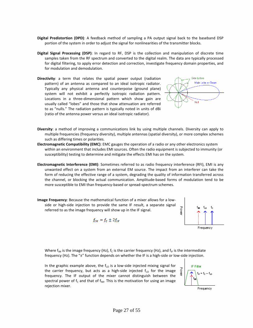
Page 27 of 55

Digital Predistortion (DPD): A feedback method of sampling a PA output signal back to the baseband DSP

portion of the system in order to adjust the signal for nonlinearities of the transmitter blocks. Digital Signal Processing (DSP): In regard to RF, DSP is the collection and manipulation of discrete time

samples taken from the RF spectrum and converted to the digital realm. The data are typically processed for digital filtering, to apply error detection and correction, investigate frequency domain properties, and for modulation and demodulation.

Directivity: a term that relates the spatial power output (radiation

pattern) of an antenna as compared to an ideal isotropic radiator. Typically any physical antenna and counterpoise (ground plane) system will not exhibit a perfectly isotropic radiation pattern. Locations in a three-dimensional pattern which show gain are usually called “lobes” and those that show attenuation are referred to as “nulls.” The radiation pattern is typically noted in units of dBi (ratio of the antenna power versus an ideal isotropic radiator).

Diversity: a method of improving a communications link by using multiple channels. Diversity can apply to

multiple frequencies (frequency diversity), multiple antennas (spatial diversity), or more complex schemes such as differing times or polarities.

Electromagnetic Compatibility (EMC): EMC gauges the operation of a radio or any other electronics system within an environment that includes EMI sources. Often the radio equipment is subjected to immunity (or susceptibility) testing to determine and mitigate the effects EMI has on the system.

Electromagnetic Interference (EMI): Sometimes referred to as radio frequency interference (RFI), EMI is any

unwanted effect on a system from an external EM source. The impact from an interferer can take the form of reducing the effective range of a system, degrading the quality of information transferred across the channel, or blocking the actual communication. Amplitude-based forms of modulation tend to be more susceptible to EMI than frequency-based or spread-spectrum schemes.

Image Frequency: Because the mathematical function of a mixer allows for a low-

side or high-side injection to provide the same IF result, a separate signal referred to as the image frequency will show up in the IF signal.

Where fIM is the image frequency (Hz), fC is the carrier frequency (Hz), and fIF is the intermediate frequency (Hz). The “±” function depends on whether the IF is a high-side or low-side injection. In the graphic example above, the fLO is a low-side injected mixing signal for the carrier frequency, but acts as a high-side injected fLO for the image frequency. The IF output of the mixer cannot distinguish between the spectral power of fC and that of fIM. This is the motivation for using an image rejection mixer.

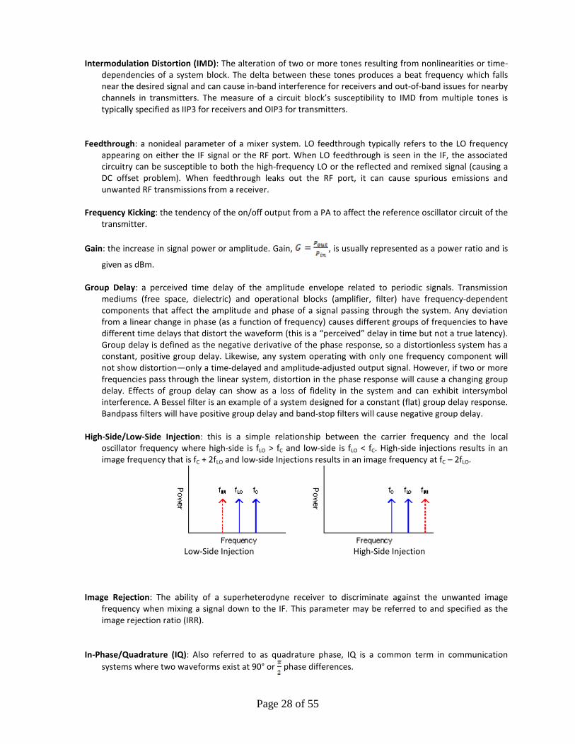
Page 28 of 55

Intermodulation Distortion (IMD): The alteration of two or more tones resulting from nonlinearities or time-dependencies of a system block. The delta between these tones produces a beat frequency which falls near the desired signal and can cause in-band interference for receivers and out-of-band issues for nearby channels in transmitters. The measure of a circuit block’s susceptibility to IMD from multiple tones is typically specified as IIP3 for receivers and OIP3 for transmitters.

Feedthrough: a nonideal parameter of a mixer system. LO feedthrough typically refers to the LO frequency

appearing on either the IF signal or the RF port. When LO feedthrough is seen in the IF, the associated circuitry can be susceptible to both the high-frequency LO or the reflected and remixed signal (causing a DC offset problem). When feedthrough leaks out the RF port, it can cause spurious emissions and unwanted RF transmissions from a receiver.

Frequency Kicking: the tendency of the on/off output from a PA to affect the reference oscillator circuit of the

transmitter. Gain: the increase in signal power or amplitude. Gain, , is usually represented as a power ratio and is

given as dBm. Group Delay: a perceived time delay of the amplitude envelope related to periodic signals. Transmission

mediums (free space, dielectric) and operational blocks (amplifier, filter) have frequency-dependent components that affect the amplitude and phase of a signal passing through the system. Any deviation from a linear change in phase (as a function of frequency) causes different groups of frequencies to have different time delays that distort the waveform (this is a “perceived” delay in time but not a true latency). Group delay is defined as the negative derivative of the phase response, so a distortionless system has a constant, positive group delay. Likewise, any system operating with only one frequency component will not show distortion—only a time-delayed and amplitude-adjusted output signal. However, if two or more frequencies pass through the linear system, distortion in the phase response will cause a changing group delay. Effects of group delay can show as a loss of fidelity in the system and can exhibit intersymbol interference. A Bessel filter is an example of a system designed for a constant (flat) group delay response. Bandpass filters will have positive group delay and band-stop filters will cause negative group delay.

High-Side/Low-Side Injection: this is a simple relationship between the carrier frequency and the local

oscillator frequency where high-side is fLO > fC and low-side is fLO < fC. High-side injections results in an image frequency that is fC + 2fLO and low-side Injections results in an image frequency at fC – 2fLO.

Low-Side Injection High-Side Injection

Image Rejection: The ability of a superheterodyne receiver to discriminate against the unwanted image

frequency when mixing a signal down to the IF. This parameter may be referred to and specified as the image rejection ratio (IRR).

In-Phase/Quadrature (IQ): Also referred to as quadrature phase, IQ is a common term in communication

systems where two waveforms exist at 90° or phase differences.

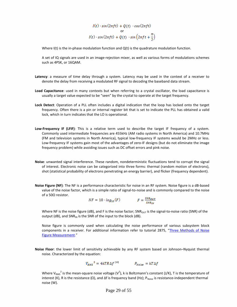
Page 29 of 55

or

Where I(t) is the in-phase modulation function and Q(t) is the quadrature modulation function. A set of IQ signals are used in an image-rejection mixer, as well as various forms of modulations schemes such as 4PSK, or 16QAM.

Latency: a measure of time delay through a system. Latency may be used in the context of a receiver to

denote the delay from receiving a modulated RF signal to decoding the baseband data stream. Load Capacitance: used in many contexts but when referring to a crystal oscillator, the load capacitance is

usually a target value expected to be “seen” by the crystal to operate at the target frequency. Lock Detect: Operation of a PLL often includes a digital indication that the loop has locked onto the target

frequency. Often there is a pin or internal register bit that is set to indicate the PLL has obtained a valid lock, which in turn indicates that the LO is operational.

Low-Frequency IF (LFIF): This is a relative term used to describe the target IF frequency of a system.

Commonly used intermediate frequencies are 455kHz (AM radio systems in North America) and 10.7MHz (FM and television systems in North America), typical low-frequency IF systems would be 2MHz or less. Low-frequency IF systems gain most of the advantages of zero-IF designs (but do not eliminate the image frequency problem) while avoiding issues such as DC offset errors and pink noise.

Noise: unwanted signal interference. These random, nondeterministic fluctuations tend to corrupt the signal

of interest. Electronic noise can be categorized into three forms: thermal (random motion of electrons), shot (statistical probability of electrons penetrating an energy barrier), and flicker (frequency dependent).

Noise Figure (NF): The NF is a performance characteristic for noise in an RF system. Noise figure is a dB-based

value of the noise factor, which is a simple ratio of signal-to-noise and is commonly compared to the noise of a 50Ω resistor.

Where NF is the noise figure (dB), and F is the noise factor; SNROUT is the signal-to-noise ratio (SNR) of the output (dB), and SNRIN is the SNR of the input to the block (dB). Noise figure is commonly used when calculating the noise performance of various subsystem block components in a receiver. For additional information refer to tutorial 2875, “Three Methods of Noise Figure Measurement.”

Noise Floor: the lower limit of sensitivity achievable by any RF system based on Johnson–Nyquist thermal

noise. Characterized by the equation:

[10]

Where VRMS2 is the mean-square noise voltage (V2), k is Boltzmann’s constant (J/K), T is the temperature of

interest (K), R is the resistance (Ω), and Δf is frequency band (Hz); PNoise is resistance-independent thermal noise (W).

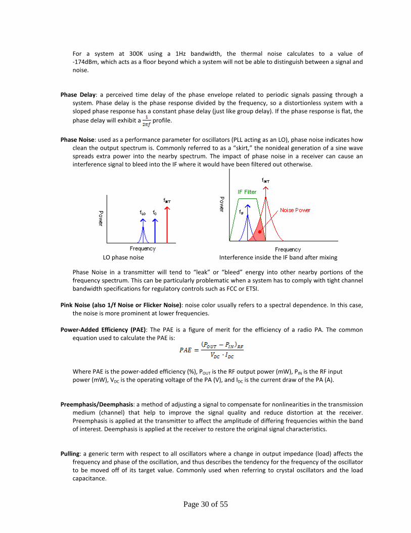
Page 30 of 55

For a system at 300K using a 1Hz bandwidth, the thermal noise calculates to a value of -174dBm, which acts as a floor beyond which a system will not be able to distinguish between a signal and noise.

Phase Delay: a perceived time delay of the phase envelope related to periodic signals passing through a

system. Phase delay is the phase response divided by the frequency, so a distortionless system with a sloped phase response has a constant phase delay (just like group delay). If the phase response is flat, the phase delay will exhibit a profile.

Phase Noise: used as a performance parameter for oscillators (PLL acting as an LO), phase noise indicates how

clean the output spectrum is. Commonly referred to as a “skirt,” the nonideal generation of a sine wave spreads extra power into the nearby spectrum. The impact of phase noise in a receiver can cause an interference signal to bleed into the IF where it would have been filtered out otherwise.

LO phase noise Interference inside the IF band after mixing

Phase Noise in a transmitter will tend to “leak” or “bleed” energy into other nearby portions of the frequency spectrum. This can be particularly problematic when a system has to comply with tight channel bandwidth specifications for regulatory controls such as FCC or ETSI.

Pink Noise (also 1/f Noise or Flicker Noise): noise color usually refers to a spectral dependence. In this case,

the noise is more prominent at lower frequencies. Power-Added Efficiency (PAE): The PAE is a figure of merit for the efficiency of a radio PA. The common

equation used to calculate the PAE is:

Where PAE is the power-added efficiency (%), POUT is the RF output power (mW), PIN is the RF input power (mW), VDC is the operating voltage of the PA (V), and IDC is the current draw of the PA (A).

Preemphasis/Deemphasis: a method of adjusting a signal to compensate for nonlinearities in the transmission

medium (channel) that help to improve the signal quality and reduce distortion at the receiver. Preemphasis is applied at the transmitter to affect the amplitude of differing frequencies within the band of interest. Deemphasis is applied at the receiver to restore the original signal characteristics.

Pulling: a generic term with respect to all oscillators where a change in output impedance (load) affects the frequency and phase of the oscillation, and thus describes the tendency for the frequency of the oscillator to be moved off of its target value. Commonly used when referring to crystal oscillators and the load capacitance.

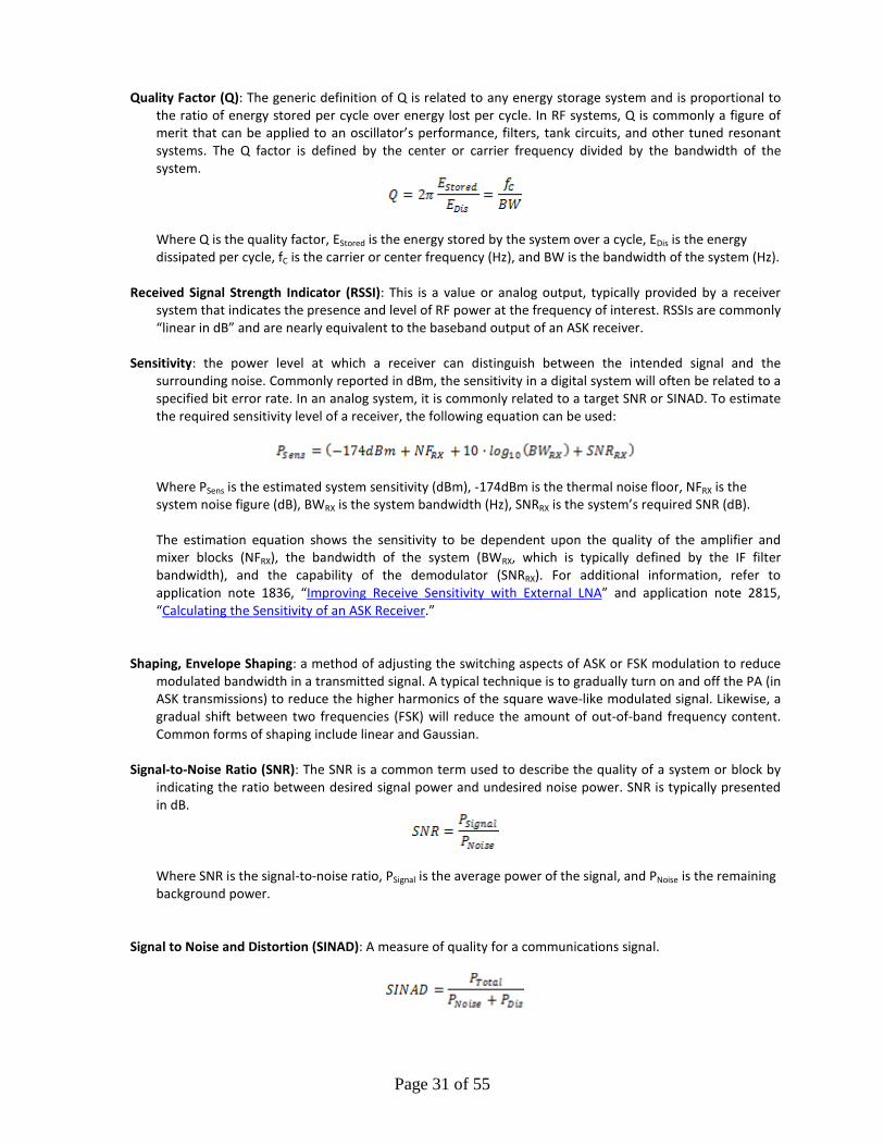
Page 31 of 55

Quality Factor (Q): The generic definition of Q is related to any energy storage system and is proportional to the ratio of energy stored per cycle over energy lost per cycle. In RF systems, Q is commonly a figure of merit that can be applied to an oscillator’s performance, filters, tank circuits, and other tuned resonant systems. The Q factor is defined by the center or carrier frequency divided by the bandwidth of the system.

Where Q is the quality factor, EStored is the energy stored by the system over a cycle, EDis is the energy dissipated per cycle, fC is the carrier or center frequency (Hz), and BW is the bandwidth of the system (Hz).

Received Signal Strength Indicator (RSSI): This is a value or analog output, typically provided by a receiver

system that indicates the presence and level of RF power at the frequency of interest. RSSIs are commonly “linear in dB” and are nearly equivalent to the baseband output of an ASK receiver.

Sensitivity: the power level at which a receiver can distinguish between the intended signal and the

surrounding noise. Commonly reported in dBm, the sensitivity in a digital system will often be related to a specified bit error rate. In an analog system, it is commonly related to a target SNR or SINAD. To estimate the required sensitivity level of a receiver, the following equation can be used:

Where PSens is the estimated system sensitivity (dBm), -174dBm is the thermal noise floor, NFRX is the system noise figure (dB), BWRX is the system bandwidth (Hz), SNRRX is the system’s required SNR (dB). The estimation equation shows the sensitivity to be dependent upon the quality of the amplifier and mixer blocks (NFRX), the bandwidth of the system (BWRX, which is typically defined by the IF filter bandwidth), and the capability of the demodulator (SNRRX). For additional information, refer to application note 1836, “Improving Receive Sensitivity with External LNA” and application note 2815, “Calculating the Sensitivity of an ASK Receiver.”

Shaping, Envelope Shaping: a method of adjusting the switching aspects of ASK or FSK modulation to reduce

modulated bandwidth in a transmitted signal. A typical technique is to gradually turn on and off the PA (in ASK transmissions) to reduce the higher harmonics of the square wave-like modulated signal. Likewise, a gradual shift between two frequencies (FSK) will reduce the amount of out-of-band frequency content. Common forms of shaping include linear and Gaussian.

Signal-to-Noise Ratio (SNR): The SNR is a common term used to describe the quality of a system or block by

indicating the ratio between desired signal power and undesired noise power. SNR is typically presented in dB.

Where SNR is the signal-to-noise ratio, PSignal is the average power of the signal, and PNoise is the remaining background power.

Signal to Noise and Distortion (SINAD): A measure of quality for a communications signal.

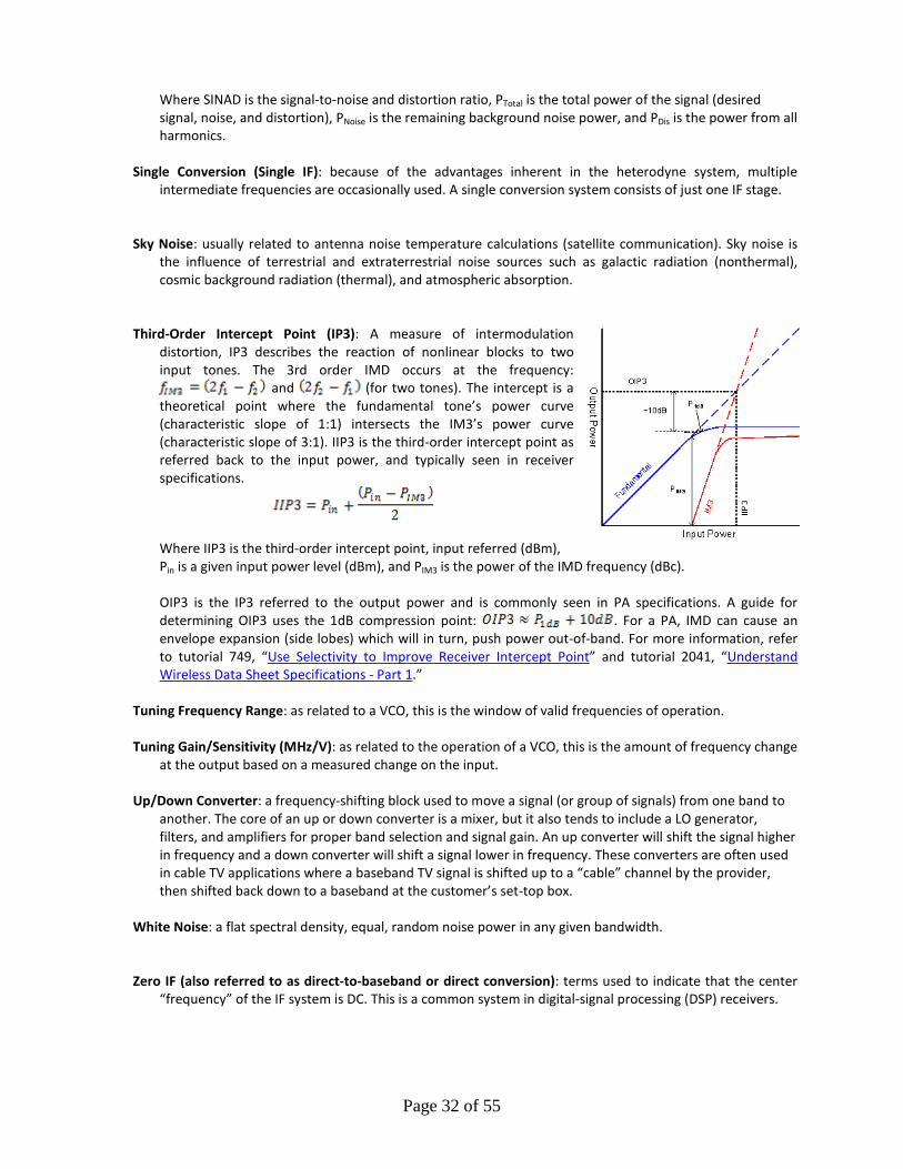
Page 32 of 55

Where SINAD is the signal-to-noise and distortion ratio, PTotal is the total power of the signal (desired signal, noise, and distortion), PNoise is the remaining background noise power, and PDis is the power from all harmonics.

Single Conversion (Single IF): because of the advantages inherent in the heterodyne system, multiple

intermediate frequencies are occasionally used. A single conversion system consists of just one IF stage.

Sky Noise: usually related to antenna noise temperature calculations (satellite communication). Sky noise is

the influence of terrestrial and extraterrestrial noise sources such as galactic radiation (nonthermal), cosmic background radiation (thermal), and atmospheric absorption.

Third-Order Intercept Point (IP3): A measure of intermodulation

distortion, IP3 describes the reaction of nonlinear blocks to two input tones. The 3rd order IMD occurs at the frequency:

and (for two tones). The intercept is a theoretical point where the fundamental tone’s power curve (characteristic slope of 1:1) intersects the IM3’s power curve (characteristic slope of 3:1). IIP3 is the third-order intercept point as referred back to the input power, and typically seen in receiver specifications.

Where IIP3 is the third-order intercept point, input referred (dBm), Pin is a given input power level (dBm), and PIM3 is the power of the IMD frequency (dBc). OIP3 is the IP3 referred to the output power and is commonly seen in PA specifications. A guide for determining OIP3 uses the 1dB compression point: . For a PA, IMD can cause an envelope expansion (side lobes) which will in turn, push power out-of-band. For more information, refer to tutorial 749, “Use Selectivity to Improve Receiver Intercept Point” and tutorial 2041, “Understand Wireless Data Sheet Specifications - Part 1.”

Tuning Frequency Range: as related to a VCO, this is the window of valid frequencies of operation. Tuning Gain/Sensitivity (MHz/V): as related to the operation of a VCO, this is the amount of frequency change

at the output based on a measured change on the input. Up/Down Converter: a frequency-shifting block used to move a signal (or group of signals) from one band to

another. The core of an up or down converter is a mixer, but it also tends to include a LO generator, filters, and amplifiers for proper band selection and signal gain. An up converter will shift the signal higher in frequency and a down converter will shift a signal lower in frequency. These converters are often used in cable TV applications where a baseband TV signal is shifted up to a “cable” channel by the provider, then shifted back down to a baseband at the customer’s set-top box.

White Noise: a flat spectral density, equal, random noise power in any given bandwidth. Zero IF (also referred to as direct-to-baseband or direct conversion): terms used to indicate that the center

“frequency” of the IF system is DC. This is a common system in digital-signal processing (DSP) receivers.

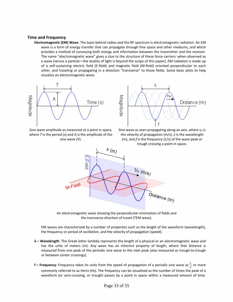
Page 33 of 55

Time and Frequency

Electromagnetic (EM) Wave: The basis behind radios and the RF spectrum is electromagnetic radiation. An EM wave is a form of energy transfer that can propagate through free space and other mediums, and which provides a method of conveying both energy and information between the transmitter and the receiver. The name “electromagnetic wave” gives a clue to the structure of these force carriers: when observed as a wave (versus a particle—the duality of light is beyond the scope of this paper), EM radiation is made up of a self-sustaining electric field (E-field) and magnetic field (M-field) oriented perpendicular to each other, and traveling or propagating in a direction “transverse” to those fields. Some basic plots to help visualize an electromagnetic wave:

Sine wave amplitude as measured at a point in space, where T is the period (s) and A is the amplitude of the

sine wave (V).

Sine wave as seen propagating along an axis, where vP is the velocity of propagation (m/s), λ is the wavelength (m), and f is the frequency (1/s) of the wave peak or

trough crossing a point in space.

An electromagnetic wave showing the perpendicular orientation of fields and

the transverse direction of travel (TEM wave). EM waves are characterized by a number of properties such as the length of the waveform (wavelength), the frequency or period of oscillation, and the velocity of propagation (speed).

λ – Wavelength: The Greek letter lambda represents the length of a physical or an electromagnetic wave and

has the units of meters (m). Any wave has an inherent property of length, where that distance is measured from one peak of the periodic sine wave to the next peak (also measured as trough-to-trough or between center crossings).

f – Frequency: Frequency takes its units from the speed of propagation of a periodic sine wave as , or more

commonly referred to as Hertz (Hz). The frequency can be visualized as the number of times the peak of a waveform (or zero-crossing, or trough) passes by a point in space within a measured amount of time.

Page 34 of 55

Frequency is also where T is the length of time or period between two peaks (or zero-crossings, or troughs) of a periodic sine wave.

T – Period: The inverse of frequency ( ), the period is the time it takes for one oscillation of a sine wave to

occur. The period uses the units of seconds (s). c – Speed of light: The speed of light in a vacuum is a physical constant with the defined value of

299,792,458m/s (one meter is defined by the distance traveled by light in a diminutive fraction of a second). Made famous by Einstein with his Theory of General Relativity, “c” had existed many years prior to his well-known formula and was first proposed by Romer, Huygens, Newton, and others as well as James Maxwell when postulating the traveling time of an electromagnetic wave. Light is mathematically represented by a sine wave with two major properties: the length of the sine wave (wavelength) and the cycle time it takes to repeat the waveform (frequency), defined by the equation[6]:

Where c is the speed of light in a vacuum (in m/s), µ0 is the magnetic permeability of free space (in H/m), ε0 is the electric permittivity of free space (in F/m), λ is the wavelength of light (in m), f is the frequency (in 1/s), and T is the period (in s).

vP – Velocity of propagation: As noted earlier, the speed of light (c) is defined by light traveling in a vacuum. In

other materials, the speed of the electromagnetic waveform may decrease. This new speed is usually referred to as the “velocity of propagation.” A more useful term in the electronics world is the velocity factor (VF), which is the ratio of the EM wave’s speed in a medium divided by the EM wave’s speed in a vacuum (represented as a percentage). Many transmission line materials provide a value for VF.

Where VF is the velocity factor (in %), vP is the velocity of propagation (in m/s), c is the speed of light in a vacuum (in m/s), µ is the magnetic permeability of the material (in H/m), and ε is the electric permittivity (in F/m).

TEM – Transverse electromagnetic wave: A transverse wave is one in which the propagation is perpendicular

to the E and M fields. TEM waves are more commonly referred to when discussing wave guides used at radio frequencies, or fiber optics when used in visible or near-visible portions of the spectrum.

Page 35 of 55

Who Controls the Use of Radios? Regulating Bodies

International Telecommunications Union (ITU): The ITU is a worldwide organizational body in the UN that manages the radio spectrum throughout the globe. As part of their structure, the ITU divides the globe into three radio regions: Europe, Africa, the Middle East, the former Soviet Union and Mongolia make up Region 1 (http://www.itu.int/ITU-R/terrestrial/broadcast/plans/ge06/index.html); the Americas and Greenland constitute Region 2 (http://www.itu.int/ITU-R/terrestrial/broadcast/plans/rj81/index.html); and Asia, Iran, Japan, the South Pacific, and Australia are in Region 3 (Asia and Pacific Regional Office, http://www.itu.int/ITU-D/asp/CMS/index.asp). [7] The regions tend to have subtle differences in frequency allocation, power limits, etc., associated with the acceptance by those states within each region. For current information on the ITU, visit www.itu.int.

Federal Communications Commission (FCC): The FCC is the federal agency of the U.S. government in charge

of regulating the use of fixed and mobile communication systems in the U.S. and by extension, North America (Region 2). The FCC receives its mandate through Title 47 of the U.S. Code (federal law, Code of Federal Regulations). The primary section of the law that governs the unlicensed ISM bands is Part 15 – Radio Frequency Devices[26]. In this document, the FCC details the operational constrains of intentional, unintentional, and incidental radiators that are permitted to operate without an individual license. It specifies technical and administrative requirement, marketing, compliance, and testing verification. It should be noted that “unlicensed” does not mean that “anything goes.” Part 15 lays out strict regulations within which any certified radio (mostly transmitters) must operate. The most prominent sections to be concerned with for the ISM bands are:

15.203 Antenna Requirements 15.209 Radiated Emission Limits, General Requirements 15.215 Additional Provisions to the General Radiated Emission Limitations 15.231 Periodic Operation in the Band 40.66-40.70MHz and Above 70MHz 15.240 Operation in the Band 433.5-434.5MHz 15.245-249 Operation in the Bands 902-928MHz, 2435-2465MHz, etc.

For additional information, refer to application notes 1772, “Where to Go for Regulations Concerning Short Range Devices (SRD)” and 3587, “FCC and ETSI Requirements for Short-Range UHF ASK-Modulated Transmitters.” For current information on the FCC, visit www.fcc.gov. European Telecommunications Standards Institute (ETSI): a standards organization based in Europe intended

to govern fixed and mobile radio communications within Region 1. Similar to FCC Part 15, ETSI provides the European Standard EN 300-220 which governs the “electromagnetic compatibility and radio spectrum matters (ERM); short-range devices (SRD); radio equipment to be used in the 25MHz to 1000MHz frequency range with power levels ranging up to 500mW”[14] (also see application note 3587, “FCC and ETSI Requirements for Short-Range UHF ASK-Modulated Transmitters”). For current information on ETSI, visit www.etsi.org.

Association of Radio Industries and Businesses (ARIB): an investigation, research and development, and

standards organization based in Japan that is focused on industry and public use of radios within that country (Region 3). The governing document from ARIB is STD-T67, Telemeter, Telecontrol, and Data Transmission Radio Equipment for Specified Low-Power Radio Stations[15]. Very broadly, the ARIB specifications are often found to be the most restrictive and difficult to comply with due to the low-power and narrow bandwidth requirements. For current information from the ARIB organization, visit http://www.arib.or.jp/english/.

Page 36 of 55

Numerous other regulatory agencies exist, commonly associated with the respective states in each region. These organizations and regulating bodies may or may not comply with ITU-established guidelines and thus should be thoroughly investigated if operation of products within those countries is anticipated. A short list of organizations by country:

India: Ministry of Communications & Information Technology (www.mit.gov.in) China: Ministry of Industry and Information Technology (www.miit.gov.cn [Chinese language site]) South Korea: Korea Communications Commission, KCC (eng.kcc.go.kr) Thailand: Post and Telegraph Department, PTD Philippines: National Telecommunications Commission (https://www.nsw.gov.ph/agencies/21) Australia: Australian Communications and Media Authority, ACMA (www.acma.gov.au)

Standards Organizations Institute for Electrical and Electronics Engineers (IEEE): The IEEE is the world’s largest professional association

dedicated to advancing technological innovation and excellence for the benefit of humanity[16]. The institute produces journals and other periodicals, sponsors conferences, hosts a digital library, and most importantly to this discussion, publishes industry standards written by various committees within the organization. For current information on the IEEE, visit www.ieee.org.

IEEE 802.11: This standard is the baseline for implementation of wireless LAN. It defines the communication

protocol (a, b, g, and n), frequency of operation, channels, bandwidth, modulation data rate, and frame structure used for interoperation by all compliant hardware. For the latest information on the IEEE 802.11 standard, visit http://grouper.ieee.org/groups/802/11/.

IEEE 802.15: This is a standard that defines the structure for personal area networks (PANs) such as Bluetooth

(Task Group 1), high- and low-rate wireless PAN (Task Groups 3 and 4), and mesh networking (Task Group 5). More commonly referred to as 802.15.4, this subsection of the standard defines the physical layer (PHY) and media access control (MAC) layer, and has been adopted as the foundation for other technology organizations’ protocols. For more information on the IEEE 802.15 standard, visit http://grouper.ieee.org/groups/802/15/.

ZigBee: a communications protocol layered on the IEEE® 802.15.4 standard for wireless mesh networking. The

ZigBee® Alliance[17] established a standard that is intended to be a protocol stack running at low data rates (250kbps) and with a secure interface, targeted at the 868MHz, 915MHz, and 2.4GHz ISM bands. ZigBee uses a carrier sense multiple access with collision avoidance (CSMA/CA) discipline, where it adds networking and security to the data link layer (DLL) of the protocol stack. For current information on the ZigBee Alliance, visit www.zigbee.org.

RF4CE (RF for Consumer Electronics): RF4CE is a specification developed by the ZigBee Alliance to provide

focused remote control interoperability of home entertainment devices, garage door openers (GDOs), and remote keyless entry (RKE) systems. The protocol operates in the 2.4GHz band of ISM and provides network and security features similar to ZigBee. Additional information can be found on the ZigBee Alliance website at www.zigbee.org.

Bluetooth, Bluetooth LE (Low Energy): the Bluetooth Special Interest Group (SIG)[18] out of Sweden defined a

packet-based protocol for the exchange of data using short range devices (SRDs). Bluetooth operates in the unlicensed 2.4GHz ISM band and has established itself as the wireless standard for computer/human interface devices. Compatible devices are broken into three groups based on their operating range (TX power): 100m, +20dBm (Class 1); 10m, +4dBm (Class 2); 5m, 0dBm (Class 3). Version 1.2 devices are capable of 1Mbps data rates, whereas v2.0 can reach 3Mbps. The latest v4.0 is host to the Bluetooth LE, which is intended to make the protocol more compatible with small-battery (coin cell) operated equipment. For current information on the Bluetooth Special Interest Group, visit www.bluetooth.com.

Wireless Meter Bus (W-MBus): The Wireless MBus is a variant on the original wired protocol (EN 13757-2)

used to facilitate remote reading of gas and electric meters. The wireless specification: EN 13757-4[19] is

Page 37 of 55

designed to operate in the European ISM band of 868MHz, defining types of communication (1-way or 2-way, fixed or mobile), data rates (4kcps, 8kcps, 32.768kcps, and 100kcps), encoding (Manchester), and the frame structure. For the latest information on the M-Bus standard, visit www.m-bus.com.

Z-Wave: is a mesh network protocol developed by the Z-Wave Alliance[20] for interoperability of “smart home”

components such as lighting control, audio/visual equipment, heating/air conditioning, and security/fire alarms. Z-Wave® radios operate in the 868MHz and 915MHz ISM bands and run at a data rate of 9.6kbps or 40kbps. Additional information can be found on the Z-Wave Alliance website at www.z-wave.com.

Internet Protocol version 6 (IPv6): IPv6 is the latest, expanded definition of the ubiquitous internet protocol

used for routed packet communication. The greatest impact of IPv6 over the current IPv4 is an expanded address space (from 32 bits to 128 bits) and use of the IPsec security scheme.

DASH7: an open-source standard for wireless sensor networking. The DASH7 protocol is intended to operate

in the 433.92MHz ISM band and at data rates from 28kbps to 200kbps. This protocol is promoted by the DASH7 Alliance[21] and is termed after the ISO/IEC 18000-7 standard, which has similarities to IEEE 802.15.4. Additional information can be found on the DASH7 Alliance website at www.dash7.org.

GSM: global system for mobile communications. A standard developed by ETSI and the GSM Association[22] to

define the second generation (2G) digital technology for use in the European cellular network. Originally targeted for the 900MHz cellular band, the network eventually expanded to operate in the 850MHz, 1.8GHz, and 1.9GHz bands as well. The system uses a time division multiple access (TDMA) channel scheme and can accommodate voice (at 13kbps) and data rates up to 1Mbps (using enhanced data rates for GSM evolution (EDGE)). For the latest information on the GSM Association, visit www.gsm.org.

Universal Mobile Telecommunications System (UMTS)/Third-Generation (3G): mobile telephone protocol for

data communication. UMTS and 3G are a family of technologies (ranging from GSM, GPRS, EDGE, WCDMA, HSPA, to LTE and LTE-Advanced) based on the ITU’s IMT2000 standard and governed by the 3GPP® standards group[23]. These cellular protocols use a form of spread-spectrum such as code division multiple access (CDMA) or wideband CDMA (WCDMA) for channelizing data. UMTS tends to use the 2.1GHz band and can reach uplink data rates as high as 22Mbps. For the latest information on the 3GPP Standards Group, visit www.3gpp.org.

Certifications

Federal Communications Commission (FCC): In addition to being the government-based regulating body for the U.S., the FCC also requires the certification of electronic products to pass a level of EMI and EMC laboratory testing. The certification indicates a product will not cause harmful emissions, any intentional radiators comply with emission limits, and that the product will not be adversely affected by EMI. Certification testing is often performed by nongovernmental laboratories.

Canadian Standards Association (CSA): An industry-based association providing standards for safety, health,

and environmental protection. For the latest information on the Canadian Standards Association, visit www.csa.ca.

Norma Oficial Mexicana (Official Mexican Standard or NOM): a Mexican product safety mark required for all

electronic products. For the latest information on NOM, visit www.economia-noms.gob.mx [Spanish language site].

C-Tick, Australian Communications Authority (ACA): A mark indicating EMC compliance with required

standards for Australia and New Zealand. Often accompanied by a “N####” mark indicating the product group standard under which the certification was received. For current information on the ACA, visit www.acma.gov.au.

Page 38 of 55

Conformité Européenne (European Conformity or “CE”): a mark used to indicate that a product has passed essential requirements (harmonized safety, environment, etc.) to be marketed in the European Economic Area (EEA). A product with the CE mark is provided free movement within the European market. For current information on the CE mark, visit ec.europa.eu/enterprise/policies/single-market-goods/cemarking/index_en.htm.

China Compulsory Certification (CCC): indicates that a product complies with safety and quality requirements

defined by the PRC government as administered by the Certification and Accreditation Administration (CNCA). For current information on the CCC and the CNCA, visit www.cnca.gov.cn [Chinese language site with an English language link].

Bureau of Standards, Metrology, and Inspection (BSMI): A Taiwan-based standards organization that must

comply with Chinese National Standards. For current information on the BSMI, visit http://www.bsmi.gov.tw [Chinese/Taiwanese language site with an English language link].

Ministry of Internal Affairs and Communications (MIC): the Japanese body that governs technical

requirements for telecommunications and radio communications. For current information on the Telecommunications Bureau of MIC, visit www.tele.soumu.go.jp/e/index.htm.

Voluntary Control Council for Interference by Information Technology Equipment (VCCI): Applicable to

equipment sold in Japan, the VCCI certification applies to ITE and indicates compliance with RF emissions standards. For current information on the VCCI Council, visit www.vcci.jp/vcci_e/.

Underwriters Laboratories (UL): A product safety certification group headquartered in Illinois. UL provides

standards for testing of products, components, etc. to assure a minimum level of human safety associated with the use of the tested products. For the latest information on UL, visit www.ul.com.

ETL (Intertek): a compliance testing organization for the North American region, a mark which indicates

adherence to electrical, gas and other safety standards. For current information on Intertek, visit www.intertek.com.

AEC-Q100: a stress qualification for integrated circuits. A sequence of qualification tests for ICs developed by

the Automotive Industry Action Group (AIAG). This is a quality assurance level expected by automotive customers to approach zero-defect reliability. For the latest information on the AIAG, visit www.aiag.org.

Where Do I Start for a Radio Design? What Frequency Should I Use? (ISM and Other Bands) Several integrated radios provided by Maxim are targeted for operation in the ISM bands. The reason for this is multifaceted; one motive is that the internationally “unlicensed” nature of these frequencies provides a large, diverse market for radio systems. Designs that comply with the standards and regulations can be used worldwide with little or no adjustment to their implementation. This portability has both advantages and disadvantages, because many would-be designers of the many and varied applications now must squeeze into the same spectrum as everyone else. With an increasingly crowded field of wireless communication and control, these narrow ISM bands can be pushed to the limit of their capabilities. When too many applications gravitate to one particular band, the old, simple methods of communication can become difficult to use. For example, the proliferation of microwave ovens tends to put a limit on the use of simple communication schemes in the 2.45GHz ISM band, while cordless phones proliferated into the 915MHz, 2.45GHz, and 5.80GHz bands so they would not interfere as much with each other’s operation. Ultimately there tends to be an optimum frequency for every application, and that frequency will likely match well with one of the ISM bands. Why then, would a designer want to operate in the 868MHz/915MHz band rather than the 433.92MHz part of the spectrum? In other words, how do you choose which frequency to design for? The answer is affected by two primary considerations: either the application has a traditional and/or predefined band in which it operates, or the

Page 39 of 55

designer must balance the tradeoffs of each parameter in the design to make the best band selection. For the various applications listed in the “Common Applications” section, the traditional band of operation is noted. That leaves a discussion of the tradeoffs considered when selecting the appropriate ISM band. Commonly the most important parameter of a new design is meeting a targeted range for the system. The answer to “which band is a better choice” would be simplified if the application had an unrestricted antenna size and placement, if the distance between radios was clear from obstructions, and if the unit was wired to line voltage supplies. If however, the application is a consumer product that must have an unexposed antenna, if its signal must penetrate walls in a home, and its system needs to run for several years off of a coin cell battery, these tradeoffs become more important. In the “Range” and “Link Budget” definitions on page 19, it was shown that the adjustment of three simple parameters can have a major impact on the operating distance. The table in the “Link Budget” section illustrates how the frequency, transmitter power, and the antenna gains were varied as a comparison exercise and resulted in estimated ranges from 57m (315MHz, +10dBm, -15dBi) to 234m (915MHz, +13dBm, -10dBi). That is a 4x difference of range based on only those three parameters. In general, the lower-frequency bands provide better range capabilities and are less dependent on line-of-sight (LOS) communication, but in practice the other impacts tend to dominate the ultimate range obtained by the system. Parameters such as the antenna size and radiation pattern, true operating environment (fewer obstructions versus worst-case planning), and the noise impact from the application surroundings tend to have the greatest influence on the actual range of the system. What about output power in these bands? How does that limit aspects like range or harmonics? By looking again at the range comparison table, the transmitter power can help compensate for a number of other deficiencies in the system. However, this must be balanced by the restrictions imposed by regulating authorities. It is very common to push the limits of the transmitter to make up for losses and inefficiencies in the antenna and matching system. To further explore path loss in RKE systems, refer to application note 3945, “Path Loss in Remote Keyless Entry Systems.” To help estimate and plan the range of a system (link budget), refer to application note 5142, “Radio Link-Budget Calculations for ISM-RF Products,” and its related Link Budget Spreadsheet. One-Way and Two-Way Systems There still exists a broad range of applications that only require a one-way communication system. For example, actions like unlocking a car door or opening the window blinds in a house do not require any form of wireless feedback. Because of this, there will always be a need for simple, cost effective, one-way wireless communication. A great majority of the applications listed in the “Common Applications” section only require one-way systems. A single-direction form of communication will likely always find a market, but as the need for monitoring, feedback, status display, and other user interactions increase, the one-way system may trend to a full transceiver arrangement. For example, in a remote keyless entry system, the user may want to make sure their vehicle is locked; or in the case of adjusting the window blinds in a house, the user may want to know what the air temperature is at the window. These are both examples of a simple one-way technology which could migrate to a two-way application. Modulation There are many styles of modulation to select from in the ISM bands. Designers tend to gravitate towards ASK in the low bands (< 470MHz portion of the IEEE UHF band) due to its ease of use and because the hardware tends to be less expensive. Alternatively, FSK got a start in the low band with tire-pressure-monitoring system (TPMS) applications; it was found to be less prone to the detrimental effects of the application environment (a rotating tire in a wheel well tends to cause AM). Any form of AM uses a linear demodulation method, so a good deal of noise gets through the system, while an FM system has better SNR with wider modulation (200kHz on a standard FM channel). However, FM loses carrier lock quickly beyond a certain sensitivity threshold (waterfall). FSK is used more prominently in the high band (> 470MHz portion of the IEEE UHF band) because of the need to meet tighter regulatory specifications. Running a frequency-base form of modulation allows the transmitter to operate as a CW signal, which cuts back on the kicking effects suffered from turning a PA on and off (ASK or OOK).

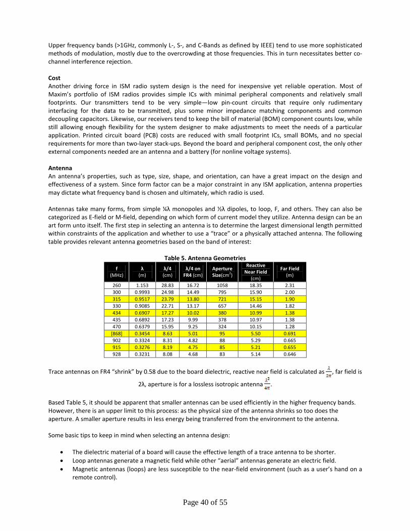
Page 40 of 55

Upper frequency bands (>1GHz, commonly L-, S-, and C-Bands as defined by IEEE) tend to use more sophisticated methods of modulation, mostly due to the overcrowding at those frequencies. This in turn necessitates better co-channel interference rejection. Cost Another driving force in ISM radio system design is the need for inexpensive yet reliable operation. Most of Maxim’s portfolio of ISM radios provides simple ICs with minimal peripheral components and relatively small footprints. Our transmitters tend to be very simple—low pin-count circuits that require only rudimentary interfacing for the data to be transmitted, plus some minor impedance matching components and common decoupling capacitors. Likewise, our receivers tend to keep the bill of material (BOM) component counts low, while still allowing enough flexibility for the system designer to make adjustments to meet the needs of a particular application. Printed circuit board (PCB) costs are reduced with small footprint ICs, small BOMs, and no special requirements for more than two-layer stack-ups. Beyond the board and peripheral component cost, the only other external components needed are an antenna and a battery (for nonline voltage systems). Antenna An antenna’s properties, such as type, size, shape, and orientation, can have a great impact on the design and effectiveness of a system. Since form factor can be a major constraint in any ISM application, antenna properties may dictate what frequency band is chosen and ultimately, which radio is used. Antennas take many forms, from simple ¼λ monopoles and ½λ dipoles, to loop, F, and others. They can also be categorized as E-field or M-field, depending on which form of current model they utilize. Antenna design can be an art form unto itself. The first step in selecting an antenna is to determine the largest dimensional length permitted within constraints of the application and whether to use a “trace” or a physically attached antenna. The following table provides relevant antenna geometries based on the band of interest:

Table 5. Antenna Geometries f

(MHz) λ

(m) λ/4 (cm)

λ/4 on FR4 (cm)

Aperture Size(cm2)

Reactive Near Field

(cm)

Far Field (m)

260 1.153 28.83 16.72 1058 18.35 2.31 300 0.9993 24.98 14.49 795 15.90 2.00 315 0.9517 23.79 13.80 721 15.15 1.90 330 0.9085 22.71 13.17 657 14.46 1.82 434 0.6907 17.27 10.02 380 10.99 1.38 435 0.6892 17.23 9.99 378 10.97 1.38 470 0.6379 15.95 9.25 324 10.15 1.28

[868] 0.3454 8.63 5.01 95 5.50 0.691 902 0.3324 8.31 4.82 88 5.29 0.665 915 0.3276 8.19 4.75 85 5.21 0.655 928 0.3231 8.08 4.68 83 5.14 0.646

Trace antennas on FR4 “shrink” by 0.58 due to the board dielectric, reactive near field is calculated as , far field is

2λ, aperture is for a lossless isotropic antenna .

Based Table 5, it should be apparent that smaller antennas can be used efficiently in the higher frequency bands. However, there is an upper limit to this process: as the physical size of the antenna shrinks so too does the aperture. A smaller aperture results in less energy being transferred from the environment to the antenna. Some basic tips to keep in mind when selecting an antenna design:

• The dielectric material of a board will cause the effective length of a trace antenna to be shorter. • Loop antennas generate a magnetic field while other “aerial” antennas generate an electric field. • Magnetic antennas (loops) are less susceptible to the near-field environment (such as a user’s hand on a

remote control).

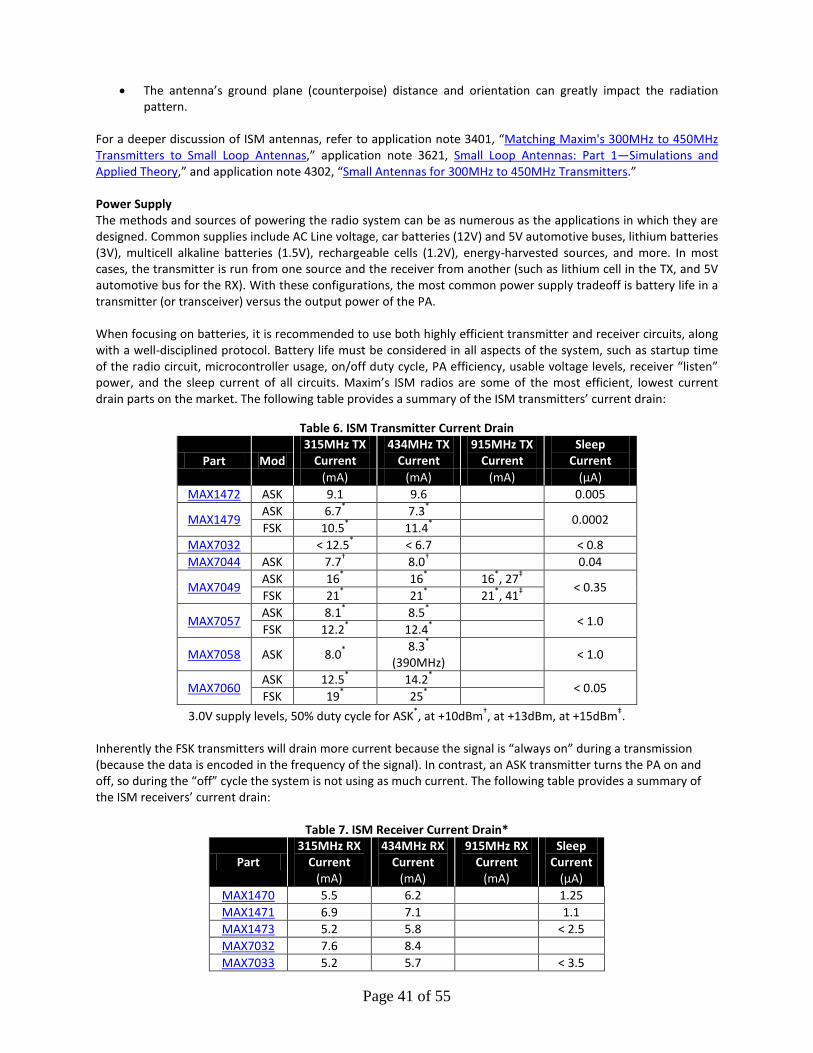
Page 41 of 55

• The antenna’s ground plane (counterpoise) distance and orientation can greatly impact the radiation pattern.

For a deeper discussion of ISM antennas, refer to application note 3401, “Matching Maxim's 300MHz to 450MHz Transmitters to Small Loop Antennas,” application note 3621, Small Loop Antennas: Part 1—Simulations and Applied Theory,” and application note 4302, “Small Antennas for 300MHz to 450MHz Transmitters.” Power Supply The methods and sources of powering the radio system can be as numerous as the applications in which they are designed. Common supplies include AC Line voltage, car batteries (12V) and 5V automotive buses, lithium batteries (3V), multicell alkaline batteries (1.5V), rechargeable cells (1.2V), energy-harvested sources, and more. In most cases, the transmitter is run from one source and the receiver from another (such as lithium cell in the TX, and 5V automotive bus for the RX). With these configurations, the most common power supply tradeoff is battery life in a transmitter (or transceiver) versus the output power of the PA. When focusing on batteries, it is recommended to use both highly efficient transmitter and receiver circuits, along with a well-disciplined protocol. Battery life must be considered in all aspects of the system, such as startup time of the radio circuit, microcontroller usage, on/off duty cycle, PA efficiency, usable voltage levels, receiver “listen” power, and the sleep current of all circuits. Maxim’s ISM radios are some of the most efficient, lowest current drain parts on the market. The following table provides a summary of the ISM transmitters’ current drain:

Table 6. ISM Transmitter Current Drain

Part Mod 315MHz TX

Current 434MHz TX

Current 915MHz TX

Current Sleep

Current (mA) (mA) (mA) (µA)

MAX1472 ASK 9.1 9.6 0.005

MAX1479 ASK 6.7* 7.3*

0.0002 FSK 10.5* 11.4*

MAX7032 < 12.5* < 6.7 < 0.8 MAX7044 ASK 7.7† 8.0† 0.04

MAX7049 ASK 16* 16* 16*, 27‡

< 0.35 FSK 21* 21* 21*, 41‡

MAX7057 ASK 8.1* 8.5*

< 1.0 FSK 12.2* 12.4*

MAX7058 ASK 8.0* 8.3* (390MHz) < 1.0

MAX7060 ASK 12.5* 14.2*

< 0.05 FSK 19* 25*

3.0V supply levels, 50% duty cycle for ASK*, at +10dBm†, at +13dBm, at +15dBm‡. Inherently the FSK transmitters will drain more current because the signal is “always on” during a transmission (because the data is encoded in the frequency of the signal). In contrast, an ASK transmitter turns the PA on and off, so during the “off” cycle the system is not using as much current. The following table provides a summary of the ISM receivers’ current drain:

Table 7. ISM Receiver Current Drain*

Part 315MHz RX

Current (mA)

434MHz RX Current

(mA)

915MHz RX Current

(mA)

Sleep Current

(µA) MAX1470 5.5 6.2 1.25 MAX1471 6.9 7.1 1.1 MAX1473 5.2 5.8 < 2.5 MAX7032 7.6 8.4 MAX7033 5.2 5.7 < 3.5

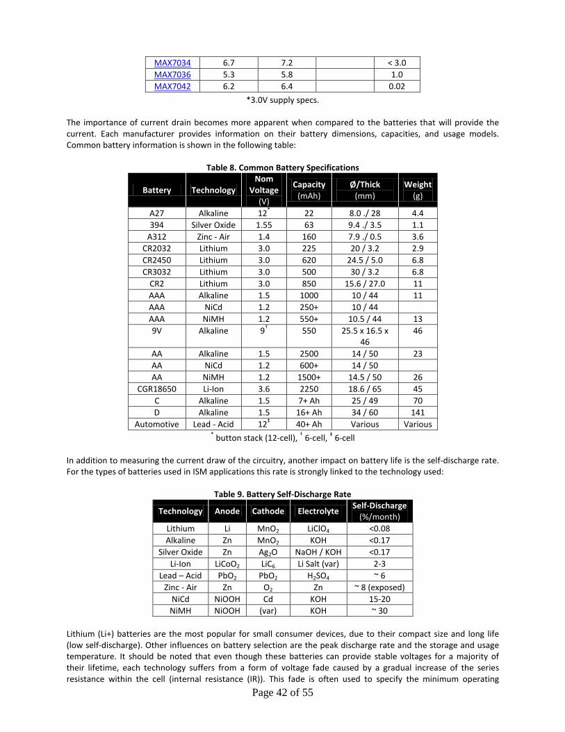
Page 42 of 55

MAX7034 6.7 7.2 < 3.0 MAX7036 5.3 5.8 1.0 MAX7042 6.2 6.4 0.02

*3.0V supply specs. The importance of current drain becomes more apparent when compared to the batteries that will provide the current. Each manufacturer provides information on their battery dimensions, capacities, and usage models. Common battery information is shown in the following table:

Table 8. Common Battery Specifications

Battery Technology Nom

Voltage (V)

Capacity (mAh)

Ø/Thick (mm)

Weight (g)

A27 Alkaline 12* 22 8.0 ./ 28 4.4 394 Silver Oxide 1.55 63 9.4 ./ 3.5 1.1

A312 Zinc - Air 1.4 160 7.9 ./ 0.5 3.6 CR2032 Lithium 3.0 225 20 / 3.2 2.9 CR2450 Lithium 3.0 620 24.5 / 5.0 6.8 CR3032 Lithium 3.0 500 30 / 3.2 6.8

CR2 Lithium 3.0 850 15.6 / 27.0 11 AAA Alkaline 1.5 1000 10 / 44 11 AAA NiCd 1.2 250+ 10 / 44 AAA NiMH 1.2 550+ 10.5 / 44 13 9V Alkaline 9† 550 25.5 x 16.5 x

46 46

AA Alkaline 1.5 2500 14 / 50 23 AA NiCd 1.2 600+ 14 / 50 AA NiMH 1.2 1500+ 14.5 / 50 26

CGR18650 Li-Ion 3.6 2250 18.6 / 65 45 C Alkaline 1.5 7+ Ah 25 / 49 70 D Alkaline 1.5 16+ Ah 34 / 60 141

Automotive Lead - Acid 12‡ 40+ Ah Various Various * button stack (12-cell), † 6-cell, ‡ 6-cell

In addition to measuring the current draw of the circuitry, another impact on battery life is the self-discharge rate. For the types of batteries used in ISM applications this rate is strongly linked to the technology used:

Table 9. Battery Self-Discharge Rate

Technology Anode Cathode Electrolyte Self-Discharge (%/month)

Lithium Li MnO2 LiClO4 <0.08 Alkaline Zn MnO2 KOH <0.17

Silver Oxide Zn Ag2O NaOH / KOH <0.17 Li-Ion LiCoO2 LiC6 Li Salt (var) 2-3

Lead – Acid PbO2 PbO2 H2SO4 ~ 6 Zinc - Air Zn O2 Zn ~ 8 (exposed)

NiCd NiOOH Cd KOH 15-20 NiMH NiOOH (var) KOH ~ 30

Lithium (Li+) batteries are the most popular for small consumer devices, due to their compact size and long life (low self-discharge). Other influences on battery selection are the peak discharge rate and the storage and usage temperature. It should be noted that even though these batteries can provide stable voltages for a majority of their lifetime, each technology suffers from a form of voltage fade caused by a gradual increase of the series resistance within the cell (internal resistance (IR)). This fade is often used to specify the minimum operating

Page 43 of 55

voltage of a radio. However, when lithium batteries reach 90% of their nominal voltage, the remaining useful current has begun to reach its limit as well. For example, when a CR2032 battery has been used for 200mAh, the internal resistance will show a doubling from the nominal value of about 15Ω to about 30Ω while the voltage has dropped from 3.0V to 2.8V. The knee at 225mAh shows the battery with an IR of around 50Ω and a supply level at 2.3V. By that time, the capacity is drained off at 240mAh, the internal resistance is over 120Ω, and the voltage has dropped below 1.8V[24]. Thus the voltage drop is a less critical aspect of the battery life than the complete loss of current capacity. Range The predicted range of system is highly dependent upon many factors, particularly operating frequency, transmitter output power, antenna efficiencies, and the receiver sensitivity. Obstacles, motion, and even atmospheric conditions can greatly influence the operating distance, but these are variables outside the control of a system designer. Thus, planning for worst-case environments usually limits the design options to TX power, antenna selection, and RX sensitivity. Transmitter output power can have the biggest impact on the range of the system. Often, higher-than-permitted power is used from the PA to make up for poor antenna efficiencies, due to smaller than 1/4-wave geometries, especially in the low bands where antenna efficiencies can be less than 10% (key fob sizes). It is important to stay within any regulatory requirements of the targeted region of operation (refer back to the Field Strength section on p.7). More power may be permitted if the duty cycle of the transmitter is varied according to the governing bodies. Some primary issues to keep in mind when selecting a PA based on output power are:

• A higher output power requires higher supply current. • The higher frequency bands require higher operating current (commonly due to PLL current). • Higher output power may impact regulatory limits such as maximum radiated power, occupied

bandwidth, and harmonic power.

Table 10 provides a summary of Maxim’s ISM transmitters’ capabilities:

Table 10. ISM Transmitter Capabilities

Part Bands (MHz)

Typical TX Power (dBm)

MAX1472 300-450 +10dBm MAX1479 300-450 +10dBm MAX7032 300-450 +10dBm MAX7044 300-450 +13dBm

MAX7049 288-945 Adjustable +15dBm

MAX7057 300-450 +10dBm

MAX7058 315 / 390 (300-450) +10dBm

MAX7060 280-450 +10dBm +14dBm*

All power specs are driving a 50Ω load and include the matching/harmonic filter loss. *With 5V supply.

On the receiver side of the system, the sensitivity is the overwhelming governor of obtainable range. Similar to the transmit side, a receiver that can pick out a signal with 3dBm less power may be able to compensate for a bad antenna or a poor link environment. The primary issues to keep in mind when selecting for a receiver’s sensitivity are:

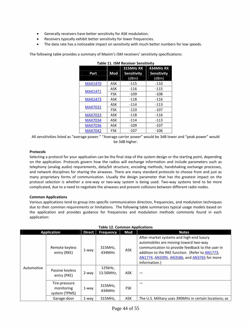
Page 44 of 55

• Generally receivers have better sensitivity for ASK modulation. • Receivers typically exhibit better sensitivity for lower frequencies. • The data rate has a noticeable impact on sensitivity with much better numbers for low speeds.

The following table provides a summary of Maxim’s ISM receivers’ sensitivity specifications:

Table 11. ISM Receiver Sensitivity

Part Mod 315MHz RX Sensitivity

(dBm)

434MHz RX Sensitivity

(dBm) MAX1470 ASK -115 -110

MAX1471 ASK -116 -115 FSK -109 -108

MAX1473 ASK -118 -116

MAX7032 ASK -114 -113 FSK -110 -107

MAX7033 ASK -118 -116 MAX7034 ASK -114 -113 MAX7036 ASK -109 -107 MAX7042 FSK -107 -106

All sensitivities listed as “average power.” “Average carrier power” would be 3dB lower and “peak power” would be 3dB higher.

Protocols Selecting a protocol for your application can be the final step of the system design or the starting point, depending on the application. Protocols govern how the radios will exchange information and include parameters such as telephony (analog audio) requirements, data/bit structure, encoding methods, handshaking exchange processes, and network disciplines for sharing the airwaves. There are many standard protocols to choose from and just as many proprietary forms of communication. Usually the design parameter that has the greatest impact on the protocol selection is whether a one-way or two-way system is being used. Two-way systems tend to be more complicated, due to a need to negotiate the airwaves and prevent collisions between different radio nodes. Common Applications Various applications tend to group into specific communication direction, frequencies, and modulation techniques due to their common requirements or limitations. The following table summarizes typical usage models based on the application and provides guidance for frequencies and modulation methods commonly found in each application:

Table 12. Common Applications Application Direct Frequency Mod Notes

Automotive

Remote keyless entry (RKE) 1-way 315MHz,

434MHz ASK

After-market systems and high-end luxury automobiles are moving toward two-way communication to provide feedback to the user in addition to the RKE function. (Refer to AN1773, AN1774, AN3395, AN3586, and AN3765 for more information.)

Passive keyless entry (PKE) 2-way

125kHz, 13.56MHz,

ASK —

Tire-pressure monitoring

system (TPMS) 1-way 315MHz,

434MHz FSK —

Garage-door 1-way 315MHz, ASK The U.S. Military uses 390MHz in certain locations; as

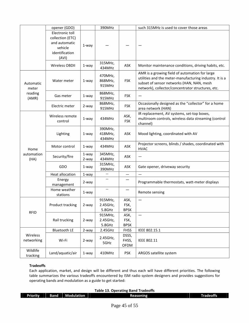
Page 45 of 55

opener (GDO) 390MHz such 315MHz is used to cover those areas Electronic toll

collection (ETC) and automatic

vehicle identification

(AVI)

1-way — — —

Wireless OBDII 1-way 315MHz, 434MHz ASK Monitor maintenance conditions, driving habits, etc.

Automatic meter

reading (AMR)

Water meter 1-way 470MHz, 868MHz, 915MHz

FSK

AMR is a growing field of automation for large utilities and the meter-manufacturing industry. It is a subset of sensor networks (HAN, NAN, mesh network), collector/concentrator structures, etc.

Gas meter 1-way 868MHz, 915MHz FSK —

Electric meter 2-way 868MHz, 915MHz FSK Occasionally designed as the “collector” for a home

area network (HAN)

Home automation

(HA)

Wireless remote control 1-way 434MHz ASK,

FSK

IR replacement, AV systems, set-top boxes, multiroom controls, wireless data streaming (control channel)

Lighting 1-way 390MHz, 418MHz, 434MHz

ASK Mood lighting, coordinated with AV

Motor control 1-way 434MHz ASK Projector screens, blinds / shades, coordinated with HVAC

Security/fire 1-way 2-way

345MHz, 434MHz ASK —

GDO 1-way 315MHz, 390MHz ASK Gate opener, driveway security

Heat allocation 1-way — — — Energy

management 2-way — — Programmable thermostats, watt-meter displays

Home weather stations 1-way

— — Remote sensing

RFID

Product tracking 2-way 915MHz, 2.45GHz, 5.8GHz

ASK, FSK, BPSK

—

Rail trucking 2-way 915MHz, 2.45GHz, 5.8GHz

ASK, FSK, BPSK

—

Wireless networking

Bluetooth LE 2-way 2.45GHz FHSS IEEE 802.15.1

Wi-Fi 2-way 2.45GHz, 5GHz

DSSS, FHSS, OFDM

IEEE 802.11

Wildlife tracking Land/aquatic/air 1-way 410MHz PSK ARGOS satellite system

Tradeoffs Each application, market, and design will be different and thus each will have different priorities. The following table summarizes the various tradeoffs encountered by ISM radio system designers and provides suggestions for operating bands and modulation as a guide to get started:

Table 13. Operating Band Tradeoffs Priority Band Modulation Reasoning Tradeoffs

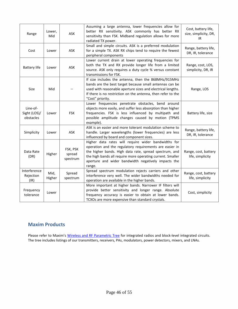
Page 46 of 55

Range Lower, Mid ASK

Assuming a large antenna, lower frequencies allow for better RX sensitivity. ASK commonly has better RX sensitivity than FSK. Midband regulation allows for more radiated TX power.

Cost, battery life, size, simplicity, DR,

IR

Cost Lower ASK Small and simple circuits. ASK is a preferred modulation for a simple TX. ASK RX chips tend to require the fewest peripheral components

Range, battery life, DR, IR, tolerance

Battery life Lower ASK

Lower current drain at lower operating frequencies for both the TX and RX provide longer life from a limited source. ASK only requires a duty cycle % versus constant transmissions for FSK.

Range, cost, LOS, simplicity, DR, IR

Size Mid —

If size includes the antenna, then the 868MHz/915MHz bands are the best target because small antennas can be used with reasonable aperture sizes and electrical lengths. If there is no restriction on the antenna, then refer to the “Cost” priority.

Range, LOS

Line-of-Sight (LOS)/

obstacles Lower FSK

Lower frequencies penetrate obstacles, bend around objects more easily, and suffer less absorption than higher frequencies. FSK is less influenced by multipath and possible amplitude changes caused by motion (TPMS example).

Battery life, size

Simplicity Lower ASK ASK is an easier and more tolerant modulation scheme to handle. Larger wavelengths (lower frequencies) are less influenced by board and component sizes.

Range, battery life, DR, IR, tolerance

Data Rate (DR) Higher

FSK, PSK spread

spectrum

Higher data rates will require wider bandwidths for operation and the regulatory requirements are easier in the higher bands. High data rate, spread spectrum, and the high bands all require more operating current. Smaller aperture and wider bandwidth negatively impacts the range.

Range, cost, battery life, simplicity

Interference Rejection

(IR)

Mid, Higher

Spread spectrum

Spread spectrum modulation rejects carriers and other interference very well. The wider bandwidths needed for operation are available in the higher bands.

Range, cost, battery life, simplicity

Frequency tolerance Lower

More important at higher bands. Narrower IF filters will provide better sensitivity and longer range. Absolute frequency accuracy is easier to obtain at lower bands. TCXOs are more expensive than standard crystals.

Cost, simplicity

Maxim Products Please refer to Maxim’s Wireless and RF Parametric Tree for integrated radios and block-level integrated circuits. The tree includes listings of our transmitters, receivers, PAs, modulators, power detectors, mixers, and LNAs.

Page 47 of 55

Examples Guidelines All ISM radio products offered by Maxim include a good typical application circuit in the product data sheet. These circuits provide a nice place to start for the design of a system. When building up a schematic for transmitters, typically the only other components necessary are a microcontroller or simple encoder interface and some form of power supply. For the receivers, a number of tuned circuits will have to be configured for the frequency of interest and data rate, in addition to the microcontroller or decoder interface and the power-supply system. For Maxim’s ISM transmitters be sure to consult these application notes:

Application note 1954, “Designing Output-Matching Networks for the MAX1472 ASK Transmitter” Application note 3401, “Matching Maxim’s 300MHz to 450MHz Transmitters to Small Loop Antennas”

For Maxim’s ISM receivers, refer to these application notes:

Application note 1017, “How to Choose a Quartz Crystal Oscillator for the MAX1470 Superheterodyne Receiver” Application note 1830, “How to Tune and Antenna” Application note 3671, “Data Slicing Techniques for UHF ASK Receivers”

Once the schematic is ready, keep in mind that most of the design problems encountered in RF systems can be traced back to a bad printed circuit board (PCB) layout. Reading up on the most common critical issues to avoid in PCB layout can save some time in the testing and debug phases of system development. Refer to tutorials 4636, “Avoid PC-Layout ‘Gotchas’ in ISM-RF Products” and 5100, “General Layout Guidelines for RF and Mixed-Signal PCBs” for more information. Application-Specific Reference Designs RC – Remote Control Reference design 5406, "LFRD004: 2-Way Remote Control Reference Design" (2-way RC) – The MAX7032 transceiver reference design (RD) is a self-contained evaluation platform for exercising the device as a simple two-way “echo” remote control demo system. The LFRD004 exhibits a two-way, 433.92MHz ASK radio communication link aimed primarily at infrared (IR) remote control replacement but can be adapted for other two-way applications such as RKE, home automation, RF sensors, or any other short-range device needs. The system uses the MAX7032 ASK/FSK transceiver on a key fob-sized board paired with a MAX610 microcontroller. AMR – Automated Meter Reading Reference design 5391, "LFRD002: Wireless Automatic Meter Reading Reference Design" (2-way meter/reader) – The MAX7032 transceiver reference design is a self-contained evaluation platform for exercising the device as a wireless automatic meter reading (AMR) demo system. The LFRD002 demonstrates a two-way, 433.92MHz ASK radio communication link aimed primarily at wireless AMR but can be adapted for other two-way applications such as energy use monitoring, home automation, remote control, remote sensing, or any other short-range device needs. The system uses the MAX7032 transceiver on both boards. Each transceiver is paired with a MAXQ610 microcontroller. Each meter radio operates in a low duty cycle sleep/listen mode until it is woken up by the reader system. Subsequently, each meter can be polled for information from one of six ports. The meters can be read individually or sequentially, as determined by the reader setup. A switch on the meter board allows the user to transmit a three-packet burst on demand. Reference design 5404, "LFRD003: Water Meter Automatic Meter Reading (AMR) Reference Design" (2-way AMR system) – The MAX7032 transceiver reference design is a modular evaluation platform for exercising the device as a wireless automatic meter reading (AMR) demo system. The LFRD003 demonstrates a two-way, 433.92MHz ASK or FSK radio communication link aimed primarily at wireless AMR. The system uses the MAX7032 ASK/FSK transceiver on a modular board, which can be used both as a stand-alone radio and as a module in conjunction with a handheld interface (HHI). Each radio module pairs the MAX7032 with a MAXQ610 microcontroller for

Page 48 of 55

independent operation and interactive control. The stand-alone radio module can be connected to a physical water meter allowing the micro to “tally” the flow count, and will store that information for later reporting on request. The HHI can control a radio module plugged into its SPI interface and subsequently use that module to interact with multiple stand-alone radios in order to query them for their stored information and to perform other utility operations. The HHI can perform utility functions such as decoding RKE, RC, or other reference design data packets; interacting with multiple remote modules; and “reprograming” select functions of the attached radio module. HA – Home Automation Reference design 5390, "LFRD014: Tube Motor Receiver Reference Design" (1-way motor control) – The MAX7034 receiver reference design is a predefined module available for use as a drop-in receiver for a tubular motor. The LFRD014 is geared towards a one-way, 433.92MHz ASK radio communication link used in a motor control system but can be adapted for other one-way applications such as RKE, remote control, RF sensing, or any other short-range device needs. The system uses the MAX7034 ASK receiver in a compact module form with antenna, power, and data connections. In most cases, these reference designs (LFRD002, LFRD003, and LFRD004) are configured such that the microcontroller can be reprogrammed in the field using the Maxim USB-to-JTAG board (MAXQUSBJTAG-KIT, ordered separately). The MAXQ610 was chosen as the primary microcontroller because of its small size, low stop-mode current consumption, and flexible DIO ports. Source code is available for all of the MAXQ610-paired systems, written in C, and developed in the IAR Embedded Workbench environment.

Page 49 of 55

For More Information Maxim provides a wealth of information available on the internet. For a sampling of additional information such as data sheets, application notes, videos, tutorials and more… Parametric tables

Transmitters: http://para.maxim-ic.com/en/search.mvp?fam=ism_tx&tree=wireless Receivers: http://para.maxim-ic.com/en/search.mvp?fam=ism_rcr&tree=wireless Transceivers: http://para.maxim-ic.com/en/search.mvp?fam=ism_tcr&tree=wireless

868MHz/915MHz ISM-Band Wireless:

http://www.maxim-ic.com/solutions/ism_band_wireless/index.mvp?CMP=relsoln Web Seminar: Wireless Technology Tutorial (Tutorial 4651):

http://www.maxim-ic.com/app-notes/index.mvp/id/4651 A list of recommended application notes:

AN686, “QPSK Modulation Demystified” AN726, “Specifying Quartz Crystals” AN742, “Impedance Matching and the Smith Chart:

The Fundamentals” AN749, “Use Selectivity to Improve Receiver

Intercept Point” AN915, “Measuring Differential Impedances with a

Two-Port Network Analyzer” AN1017, “How to Choose a Quartz Crystal Oscillator

for the MAX1470 Superheterodyne Receiver” AN1018, “How to Modify an Existing Design from a

TDA5200 or TDA5201 to a MAX1470 Superheterodyne Receiver”

AN1759, “LNA Tuned for the 433.05MHz to 434.79MHz European ISM Band”

AN1772, “Where to Go for Regulations Concerning Short-Range Devices (SRD)”

AN1773, “Designing Remote Keyless Entry (RKE) Systems”

AN1774, “Remote Keyless Entry Systems Overview” AN1776, “MAX1470 Superheterodyne Receiver FAQ” AN1830, “How to Tune and Antenna Match the

MAX1470 Circuit” AN1836, “Improving Receiver Sensitivity with

External LNA” AN1913, “Improved Device S-Parameter

Measurement with Fixture Design and Calibration” AN1954, “Designing Output-Matching Networks for

the MAX1472 ASK Transmitter” AN1955, “Fast Start-Up Oscillator (FOX) Boosts

Superhet Performance”

AN2041, “Understanding Wireless Data Sheet Specifications”

AN2815, “Calculating the Sensitivity of an ASK Receiver”

AN2875, “Three Methods of Noise Figure Measurement”

AN3395, “Requirements of Remote Keyless Entry (RKE) Systems”

AN3401, “Matching Maxim’s 300MHz to 450MHz Transmitters to Small Loop Antennas”

AN3435, “Manchester Data Encoding for Radio Communications”

AN3469, “Building a Low-Cost White-Noise Generator”

AN3571, “S-Parameter Measurements and Stability Analysis for the MAX2640 LNA”

AN3587, “FCC and ETSI Requirements for Short-Range UHF ASK-Modulated Transmitters”

AN3589, “Power Amplifier Theory for High-Efficiency Low-Cost ISM-Band Transmitters”

AN3621, “Small Loop Antennas: Part 1—Simulations and Applied Theory”

AN3671, “Data Slicing Techniques for UHF ASK Receivers”

AN3815, “Radiated Power and Field Strength form UHF ISM Transmitters”

AN3945, “Path Loss in Remote Keyless Entry Systems”

AN4302, “Small Antennas for 300MHz to 450MHz Transmitters”

AN4439, “I’m OOK. You’re OOK?”

Page 50 of 55

AN4636, “Avoid PC-Layout ‘Gotchas’ in ISM-RF Products”

AN5100, “General Layout Guidelines for RF and Mixed-Signal PCBs”

AN5142, “Radio Link-Budget Calculations for ISM-RF Products”

FCC The United States Frequency Allocation Chart can be found here:

http://www.ntia.doc.gov/files/ntia/publications/2003-allochrt.pdf Part 15 can be found in HTML format: http://transition.fcc.gov/oet/info/rules/ and in PDF format:

http://www.gpo.gov/fdsys/pkg/CFR-2009-title47-vol1/pdf/CFR-2009-title47-vol1-part15.pdf

References

1. Isaac Newton, 5 Feb 1676 in a letter to Robert Hooke.

2. Maxwell, James Clerk. A Dynamical Theory of the Electromagnetic Field, Received 27 Oct Read 8 Dec 1864, published 1865 Philosophical Transactions of the Royal Society of London 155: pp459-512.

3. Wireless Telegraphy, Patent No. 711,130, Harry Shoemaker, Filed 16 Oct 1901, Patented 14 Oct 1902, U.S.

Patent Office, http://www.google.com/patents?id=paBtAAAAEBAJ.

4. Superheterodyne Receiver, Patent No. 2,027,986, Rupert I. Kinross, Filed 10 Nov 1933, Patented 14 Jan 1936, U.S. Patent Office, http://www.google.de/patents/about?id=6cBBAAAAEBAJ.

5. United States Frequency Allocations, U.S. Department of Commerce, © Oct 2003.

6. Marshall, Stanley V. and Skitek, Gabriel G. Electromagnetic Concepts and Applications, © 1990, Prentice-

Hall Inc., p330.

7. “ITU Regional Presence,” International Telecommunication Union. www.itu.int/net/ITU-SG/regional.aspx, accessed 22 March 2012.

8. Ziemer, Rodger E. and Peterson, Roger L. Introduction to Digital Communications © 1992, Macmillan

Publishing Company, p8.

9. Murata CERAFIL SFECV-type filters, based on part SFECV10M7HA00-R0, P61E7.pdf 01.10.17.

10. Ziemer, R. E. and Tranter, W. H. Principles of Communications – Systems, Modulation, and Noise © 1990, Houghton Mifflin Company, p752.

11. A short biography of Phillip H. Smith can be found at http://www.sss-mag.com/smith01.html#bio.

12. BesserNet™ matching applet, Besser Associates, © 1999-2006,

http://www.bessernet.com/jobAids/jSmith/jSmith.html.

13. RFdude.com Smith Chart Program, RFdude.com LLC, Lance Lascari, © 2008-2010, v0.810, Jun 2007 http://tools.rfdude.com/RFdude_Smith_Chart_Program/RFdude_smith_chart_program.html.

14. ETSI EN 300 220-1 v2.3.1 (2009-04), European Telecommunications Standards Institute, © 2009,

http://www.etsi.org/.

Page 51 of 55

15. ARIB STD-T67, Association of Radio Industries and Businesses, Version 1.1 (English Translation), © 30 Nov 2005, http://www.arib.or.jp/english/html/overview/st_ej.html.

16. Institute for Electrical and Electronics Engineers. About the IEEE. © 2011,

http://www.ieee.org/about/index.html. 17. ZigBee is a registered trademark of the ZigBee Alliance. http://www.zigbee.org/Specifications.aspx.

18. Bluetooth is a registered trademark of the Bluetooth SIG. http://www.bluetooth.org/.

19. EN 13757-4:2005, Communication Systems for Meters and Remote Reading of Meters – Part 4: Wireless

Meter Readout, © 28 Oct 2005, BSI Group / ANSI, http://shop.bsigroup.com/ProductDetail/?pid=000000000030096182 / http://webstore.ansi.org/RecordDetail.aspx?sku=DIN+EN+13757-4:2005.

20. Z-Wave is a registered trademark of the Z-Wave Alliance. http://www.z-wave.com/. 21. http://www.dash7.org/.

22. http://www.gsm.org/.

23. 3GPP is a registered trademark and a registered service mark of the European Telecommunications

Standards Institute. http://www.3gpp.org/.

24. Energizer CR2032 Product Datasheet, Form No EBC-4120J, © Energizer Holdings Inc., © 2009.

25. Federal Communications Commission. Part 15 – Radio Frequency Devices © 10 Jul 2008, http://transition.fcc.gov/oet/info/rules/.

Wi-Fi is a registered certification mark of Wi-Fi Alliance Corporation.

Page 52 of 55

All other trademarks are the property of their respective owners. All rights reserved.

Page 53 of 55

Index

1dB compression point…………………..26 3G………………………………………...37 ACA……………………………………...37 Adjacent channel power…………………..9 Admittance……………………………….14 AEC-Q100……………………………….38 AES128…………………………………..12 Amplitude shift keying…………………..17 Analog front-end…………………………20 Anechoic chamber……………………….13 Antenna……………..4, 5, 13, 20, 35, 40, 47 Aperture……………………………...26, 40 Attenuator………………………………..13 Automatic gain control…………………..26 Automotive………………………38, 42, 44 Band……………………………………….9 Bandwidth…………………………………9 Baseband…………………………………26 Battery life……………………….24, 41, 46 Lithium…………………………………...42 Bias inductor …………………………….26 Bit-error rate ……………………………..26 Blocker…………………………………...26 Bluetooth……………………..10, 17, 36, 45 Capacitance………………………………15 Capacity………………………….18, 41, 42 Carrier……………………………………..8 Channel……………………………………9 Charge pump……………………………..20 Checksum………………………………...11 Coax……………………………………...13 Co-Channel Interference…………………..9 Complex Conjugate………………………………15 Number………………………………...14 Conductance……………………………...15 Constellation diagram……………………27 Continuous wave………………………4, 17 Conversion……………………………….32 Cost…………………………………..39, 46 CSA………………………………………37 Cyclic redundancy check………………...12 DASH7…………………………………...37 Data rate……………………………...17, 46 Data slicer………………………………..21

Decibels……………………………………7 Deemphasis………………………………30 Digital predistortion……………………...27 Digital signal processing…………………27 Directivity………………………………..27 Diversity………………………………….27 Divider…………………………………...21 Fractional-N……………………………...21 Down converter…………………………..32 Effective isotropic radiated power………...8 Electromagnetic compatibility…………...27 Electromagnetic interference…………….27 Electromagnetic wave ………………3, 6, 33 Encoding…………………………………11 Manchester……………………………….11 Encryption………………………………..12 Envelope shaping………………………...31 Error detection…………………………...11 ETSI………………………6, 30, 35, 37, 49 Faraday Cage…………………………….13 Far-field……………………………...20, 40 FCC…………..6, 8, 9, 10, 30, 35, 37, 50, 51 Feedthrough……………………………...28 Field strength……………………………...7 Filter Data…………………………………….20 Loop……………………………………23 Sallen-Key……………………………...20 Frequency…………………………….34, 38 Demodulator…………………………...21 Deviation…………………………….....18 Domain………………………………8, 12 Shift keying………………………...17, 18 Friis Equation…………………………….19 Gain…………………………..16, 23, 24, 28 Gilbert cell……………………………….23 Group delay………………………………28 GSM……………………………………...37 Harmonic…………………………………9 Hertz………………………………...3, 4, 34 IEEE 802.11………………………………36, 45 802.15………………………………36, 45 Image frequency………………………….27 Image rejection…………………………...28

Page 54 of 55

Imaginary…………………………….14, 15 Impedance………………………………..14 Inductance………………………………..15 Injection………………………………….28 Insertion loss……………………………..16 Intermediate frequency Amplifier……………………………5, 22 Low-frequency IF……………………...29 Zero IF…………………………………33 Intermodulation distortion……………….28 IPv6………………………………………37 ISM…………………………………..10, 49 ISM bands ……………………………….38 ITU………………………………...6, 35, 37 Kicking…………………………………...28 Latency…………………………………...29 Limiting amp……………………………..22 Line of sight………………………….38, 46 Link budget…………………………..19, 39 Load capacitance…………………………29 Lobes……………………………………..10 Lock detect……………………………….29 Lossy……………………………………..16 Low-noise amplifier…………………..5, 23 Matching…………………………………13 Maxwell………………………………3, 34 Mixer…………………………………….23 Image rejection…………………………..22 Modulation…………………………...16, 39 ASK…………..4, 5, 22, 31, 39, 41, 44, 49 CW…………………………………..4, 39 Depth…………………………………...17 FSK……………...4, 17, 22, 31, 39, 41, 44 OOK…………………………...4, 17, 39, 49 PWM……………………………………..11 Modulator………………………………….4 Near-field communication……………….10 Near field…………………………….20, 40 Newton………………………………...3, 34 Noise……………………………………..29 Flicker……………………………...29, 30 Noise floor……………………………..30 Pink…………………………………….30 Shot…………………………………….29 Sky……………………………………..32 Thermal………………………………...30 White…………………………………...33 Noise figure………………………………29 NOM……………………………………..37

Nyquist…………………………………...30 One-way……………………………...39, 44 Oscillator Crystal………………………………….20 Local………………………………...5, 22 Pierce…………………………………...20 Reference……………………………4, 24 TCXO………………………………20, 46 Voltage controlled……………………...25 Parity……………………………………..11 Peak detector……………………………..23 Period…………………………………….34 Phase delay……………………………….30 Phase-frequency detector………………...24 Phase lock loop…………………………..24 Phase noise……………………………….30 Power……………………………………...7 Power-added efficiency………………….30 Power amplifier……………………4, 24, 49 Power density…………………………….18 Power meter……………………………...13 Preemphasis……………………………...30 Protocols…………………………………44 Pulling……………………………………31 Quadrature………………………………..29 Quality factor…………………………….31 Range……….........19, 35, 36, 38, 43, 46, 49 Reactance………………………………...14 Real………………………………………14 Receiver…………………………………...5 Reflection coefficient…………………….16 Remote control……………………….11, 45 Resistance………………………………..14 Return loss……………………………….16 Return to zero…………………………….11 Reverse isolation…………………………16 RF4CE…………………………………...36 RFID…………………………………10, 45 RKE………………………19, 36, 39, 44, 49 RSSI……………………………………...31 Sensitivity……………………………31, 44 Short-range devices………………………10 Sideband………………………………….10 Signal to noise and distortion…………….32 Signal-to-noise ratio……………………...31 Smith Chart………………………………13 Sniffer……………………………………13 S-parameters……………………………..15 Spectrum…………………………………..6

Page 55 of 55

Speed of light…………………………….34 Spread spectrum……………………...18, 46 Spurs……………………………………..10 Standing wave ratio………………………16 Superheterodyne…………..5, 23, 28, 29, 49 Susceptance………………………………15 Tank circuit………………………………25 TEM cell…………………………………13 Third-order intercept point………………32 Time domain……………………………..12 TPMS…………………………….39, 44, 46 Tradeoffs…………………………………45 Transceiver………………………………...5 Transmission line………………………...25 Transmitter………………………………...4 Transverse electromagnetic……………...34

Tuning……………………………………32 Two-way……………………………..39, 44 UL………………………………………..41 UMTS……………………………………37 Up converter……………………………..32 Variable gain amplifier…………………..25 VCO……………………………………...25 Velocity of propagation………………….34 Voltage……………………………………7 Wavelength………………………………33 Whitening………………………………...11 Wireless personal area networks…………10 W-MBus………………………………….36 ZigBee ……………………………………36 Z-Wave…………………………………..36