Maximizing the rate of return on the capital employed in ...isidl.com/wp-content/uploads/2017/07/E4420-ISIDL.pdfMaximizing the rate of return on the capital employed in shipping capacity

Omega ∎ (∎∎∎∎) ∎∎∎–∎∎∎

Contents lists available at ScienceDirect

Omega

http://d0305-04

☆ThisE-m

kjetil.fagjorgen.r

Pleas(2016

journal homepage: www.elsevier.com/locate/omega

Maximizing the rate of return on the capital employed in shippingcapacity renewal$

Ove Mørch a, Kjetil Fagerholt a, Giovanni Pantuso a,b, Jørgen Rakke c,d

a Department of Industrial Economics and Technology Management, Norwegian University of Science and Technology, Trondheim, Norwayb Department of Mathematical Sciences, University of Copenhagen, Copenhagen, Denmarkc Norwegian Marine Technology Research Institute (MARINTEK), Trondheim, Norwayd Department of Marine Technology, Norwegian University of Science and Technology, Trondheim, Norway

a r t i c l e i n f o

Article history:Received 7 October 2015Accepted 16 March 2016

Keywords:Return on capital employedCapacity expansionFleet renewalMaritime transportation

x.doi.org/10.1016/j.omega.2016.03.00783/& 2016 Elsevier Ltd. All rights reserved.

manuscript was processed by Associate Editoail addresses: [email protected] (O. Mørch),[email protected] (K. Fagerholt), pantuso@[email protected] (J. Rakke).

e cite this article as: Mørch O, et al.), http://dx.doi.org/10.1016/j.omega.

a b s t r a c t

Decisions regarding investments in capacity expansion/renewal require taking into account both theoperating fitness and the financial performance of the investment. While several operating requirementshave been considered in the operations research literature, the corresponding financial aspects have notreceived as much attention. We introduce a model for the renewal of shipping capacity which maximizesthe Average Internal Rate of Return (AIRR). Maximizing the AIRR sets stricter return requirements onmoney expenditures than classic profit maximization models and may describe more closely shippinginvestors' preferences. The resulting nonlinear model is linearized to ease computation. Based on datafrom a shipping company we compare a profit maximization model with an AIRR maximization model.Results show that while maximizing profits results in aggressive expansions of the fleet, maximizing thereturn provides more balanced renewal strategies which may be preferable to most shipping investors.

& 2016 Elsevier Ltd. All rights reserved.

1. Introduction

Among the most crucial decisions for a shipping company, thecomposition of the fleet of ships determines, to a great extent, thecompetitiveness of the company. Finding the best adaption of thefleet to volatile market conditions is the main scope of the Mar-itime Fleet Renewal Problem (MFRP), which consists of decidinghow many and which types of ships to add to the fleet and whichavailable ships to dispose of (see, e.g., [3,30,31]).

The MFRP can be considered a special version of the CapacityExpansion Problem (CEP) or of the Machine Replacement Problem(MRP). CEPs seek the best addition to available capacity in order tomeet increasing demand, while MRPs seek the best substitution ofavailable machines, induced by factors such as obsolescence [29],deterioration, and ageing. In CEPs and MRPs the terms “capacity”and “machine” generically refer to equipment of various types,such as, cables, pumps, computers, and vehicles [33], with differ-ences in, for example, economic life, cost magnitude, and rele-vance for the core business.

CEPs and MRPs have received considerable attention by theoperations research community, producing a plethora of models at

r Salazar-Gonzalez.

ath.ku.dk (G. Pantuso),

Maximizing the rate of retu2016.03.007i

increasing level of realism, and adapting to various operatingconfigurations. For example, Fong and Srinivasan [12] considermulti-period capacity expansion and location, Li and Tirupati [22]focus on the trade-off between specialized and flexible capacity inmulti-product production systems, Cormier and Gunn [10] con-sider warehouse capacity expansion under inventory constraints,Kimms [19] combines capacity expansion with production plan-ning and lot sizing, van Ackere et al. [40] study the short-termproblem of adjusting the capacity in reaction to the behavior ofcustomers waiting in queues, while Ahmed et al. [2] and Bean et al.[4] study CEPs under uncertainty. The main issues faced in CEPsare related to expansion size, time, and location [24] and theoption of replacing machines is typically ignored [33]. As far asMRPs are concerned, Sethi and Chand [37] consider the replace-ment of single machines with only one replacement alternative,while Chand and Sethi [6] allow the possibility of replacingavailable machines by any from a set of available alternatives.Goldstein et al. [14], Nair and Hopp [29], Hopp and Nair [16], andAdkins and Paxson [1] consider replacement decisions triggeredby technological breakthroughs. Typically, MRPs do not considerthe possibility of changes in the demand for equipment. Capacityexpansions and replacements are however naturally tied decisions(see, e.g., [34,33,35,7]).

The problem of expanding/replacing transportation capacitytakes on specific features due to the interplay between theinvestment in vehicles and their routing. Classical models focus

rn on the capital employed in shipping capacity renewal. Omega

www.sciencedirect.com/science/journal/03050483

www.elsevier.com/locate/omega

http://dx.doi.org/10.1016/j.omega.2016.03.007



mailto:[email protected]








O. Mørch et al. / Omega ∎ (∎∎∎∎) ∎∎∎–∎∎∎2

mainly on the initial configuration of a fleet of vehicles (see, e.g.,[11] and the surveys in [15,30]), rather than its evolution. However,the problem of renewing fleets of vehicles has recently receivedattention especially in the maritime literature, due to the volatilenature of the shipping business, and the consequent need to adjustshipping capacities in response to changes in the market. As anexample, Alvarez et al. [3] and Pantuso et al. [31] consider multi-period renewal of a fleet of ships in order to cope with uncertainmarket developments. Examples can also be found for rail-roadcapacity expansions (see, e.g., [23]).

The studies mentioned above cover a wide variety of operatingfeatures and equipment types. However, relatively little attentionhas been paid by the operations research community to thefinancial aspects related to investments in capacity besides theirtechnical fitness. Most of the models available seek minimum costor maximum profit capacity expansion/replacement decisionswith the Net Present Value (NPV) being the only metric used.However, financial and economic data related to an investmentcan be aggregated in a number of alternative ways, giving rise todifferent metrics often used in place of, or in conjunction with, theNPV for evaluating the profitability of capital asset investments(see, e.g., [36,27]). This is especially true for equipment with longeconomic life and a relevant capital magnitude, such as vehicles,buildings, and pipelines. As an example, Menezes et al. [28],pointing out that a mere attention to profit in facility location canlead to too high investments, include Return on Investmentthresholds requirements in the corresponding models, and showthat this leads to a higher utilization of the available facilities.Particularly, for the case of maritime shipping, Stopford [38] showsthat investments can be evaluated by the ratio between the eco-nomic value added by the transportation services over the netasset value of the fleet.

In this paper, we consider the maximization of the AverageInternal Rate of Return (AIRR) in the renewal of maritime shippingcapacity. The AIRR [25] measures the return of multi-periodinvestment projects which generalizes and solves a number offlaws of the well known concept of Internal Rate of Return (IRR) asexplained by Magni [26]. It can be expressed as the ratio betweenthe actualized returns generated by a stream of capital invest-ments over the actualized sum of the investments. This metric is inline with the indicator used in Stopford [38]. The focus is on theMFRP as it well represents strategic CEPs and MRPs due to the longeconomic life of ships, their cost magnitude, and the high level ofuncertainty. As an example, the second-hand price of a five yearold 300 000 deadweight tons (dwt – a standard measurement unitfor the ship carrying capacity) oil tanker, increased from 124 to145 million dollars in 2008, and fell down again to 84 milliondollars in 2009 as reported by the United Nations Conference onTrade and Development [39]. The contribution of this paper istherefore twofold: (1) we introduce a model for maximizing theAIRR for capacity renewal in shipping, and (2) we compare theresults of the new model against that of a more classic modelmaximizing profits NPV in order to offer managerial insights byhighlighting the economical and structural differences in thesolutions obtained. In addition, we show how the resulting non-linear AIRR model can be reformulated in an equivalent linearmodel in order to ease computation. In order to account for mar-ket information being revealed at different points in time, both theAIRR and the profit maximization problems are formulated asmultistage stochastic programs.

The remainder of this paper is organized as follows. In Section 2we provide a thorough description of the MFRP. In Section 3 weintroduce a mathematical model for the MFRP which maximizesthe AIRR, as well as an alternative model which maximizes profits.In Section 4 we analyze the results and the solutions obtained by

Please cite this article as: Mørch O, et al. Maximizing the rate of retu(2016), http://dx.doi.org/10.1016/j.omega.2016.03.007i

the two alternative models based on the case of a major linershipping company. Finally, conclusions are drawn in Section 5.

2. The renewal of maritime shipping capacity

The MFRP is a special version of MRPs and CEPs due to routingconstraints. The objective is to seek an investment mix which issound in some economical sense (typically cost efficient) andrespects operating constraints. In what follows, we sketch themain features of the problem, while a detailed description can befound in Pantuso et al. [31].

The MFRP consists of deciding, for each time period, how manyships of each type to add to or remove from the available fleet.Ships can be bought in the second-hand market, or built. In theformer case, the company must choose from the ships available inthe market but the ship is available in short time (typically weeksto months). In the latter case the ship can be built according to thecompany's specifics but the building process takes longer time(typically years). Ship prices depend, to a great extent, on the typeof ship, its age, and on the market status. Ships can be disposed ofby selling them in the second-hand market or scrapping (demol-ishing) them. In both cases the ship can be removed from the fleetin weeks to months. Scrapping rates depend to a great extent onthe weight of the steel the ship is made of, and are thereforesensitive to changes in steel prices.

A necessary distinction must be made. In the shipping businessthere exist two broad types of players interested in investing in ships,which we will refer to as speculators and ship operators. Speculatorssee ships as an asset to trade. Their main scope is buying ships inorder to sell them at a higher price when the market allows so. Theydo not necessarily have competencies in shipping operations, but seeships as a marketable asset. Ship operators, on the contrary, buy shipsto operate them. Their business model consists of using ships toprovide transportation services. Finer classifications, though possible,are beyond the scope of this paper. In what follows we refer to theship operator type of player.

When deciding how to modify the available fleet, investorsmust take into account how the fleet is operated. This includesboth the possibility of temporary adjustments to the fleet and theutilization (i.e., the sailing activities) of the available fleet. Tem-porary adjustments to the fleet are mainly done by means of timecharters, which consist of hiring a ship and its crew for a periodtime (weeks to years). The charterer pays a (per day) fee as well asall sailing-related expenses, such as fuel and port fees. The ownerof the ship bears the rest of the costs, such as capital cost, crew,and insurance. Any shipping company can, in general, act both as acharterer and a charteree, depending on the specific need. Fleetscan also be temporarily scaled down by laying-up ships, whichconsists of stopping ships at port for a period of time, paying portfees but reducing operating expenses such as manning, storages,and, possibly, insurance.

The utilization of the ships depends on the shipping company'soperation mode (see, e.g., [21,9]). In what follows we focus,without much loss of generality (see [31]) on liner shippingoperations. Liner shipping companies deploy their fleets on anumber of trades. A trade is a sequence of origin and destinationports in different geographic areas (e.g., Europe to U.S. and Asia toEurope). A ship deployed (i.e., assigned) to a trade (servicing thetrade) visits some/all of the ports on the trade according to a pre-published schedule, picking up cargoes at origin ports and deli-vering cargoes at destination ports. Concluded the sailing on onetrade, the ship is deployed on another/the same trade with, pos-sibly, some empty (ballast) sailing to reposition the ship. Trades areseparated into contractual and optional trades. On contractualtrades the shipping company has contractual transportation





O. Mørch et al. / Omega ∎ (∎∎∎∎) ∎∎∎–∎∎∎ 3

agreements to be fulfilled while on optional trades no contractualagreement exists. However, the company may, as a strategicdecision, choose to start servicing optional trades at any time inthe future. This usually corresponds to a long-term commitmentequivalent to entering a new market. For most trades the companymay wish to ensure a certain number of services per year (fre-quency) in order to establish a presence in a given market or tosatisfy customers requirements.

3. Mathematical models

In this section, after discussing specific modeling assumptionsin Section 3.1, and introducing the notation in Section 3.2, wepropose two alternative mathematical models for the MFRP. InSection 3.3 we introduce a model for the maximization of theAIRR. Since the model in Section 3.3 is a mixed-integer nonlinearstochastic program in Section 3.4 we show how the model can belinearized to ease computation. Finally, in Section 3.5 we introducea profit NPV maximization model.

3.1. Modeling assumptions

The mathematical models presented in Sections 3.5 and 3.3have been adapted from the cost minimization model presented inPantuso et al. [31], where the reader can find specific details. Weassume that our models are tailored for liner shipping of rollingequipment. However, the models do not lose (much) generality, asthey can be readily used for (or adapted to) different maritimetransportation modes and types of cargoes, as explained in Pan-tuso et al. [31]. Here we mention a few elements necessary forintroducing the models.

Trades are organized in loops. A loop is an ordered sequence oftrades. In the model, ships are assigned to loops. Assigning a shipto a loop corresponds to having the ship servicing the trades of theloop in the specified order. Ballast sailing between the trades inthe loop (empty ship repositioning) is possible and accounted forin the duration of loop. No transhipment (i.e., movement of car-goes from a ship to another) is considered. Given its strategicrelevance, we assume that if the shipping company chooses toservice an optional trade in a period, it must continue to servicethe trade for the rest of the planning horizon. We also assume thatdifferent types of cargoes (rolling equipment) need to be trans-ported, as is typical in this shipping segment. Therefore, ships havea capacity (maximum allowance) for each cargo type as well as atotal capacity which must be respected. Examples will be given forthe specific case study in Section 4.1.

The cost of the capital necessary for buying a ship is, in general,affected by the way the company chooses to finance the ship.Alternative financing decisions (see [38] for an overview) will notbe considered. Rather, the cost of the capital is included in thecosts of the ship. When a ship is built/bought, we consider oneunique payment at purchase time. This can in practice representboth the actualized sum of future installments (e.g., debt repay-ment and interests) and an actual (less likely) upfront cash pay-ment, or a combination of these. Similarly, when a ship is sold/scrapped we assume that the company receives one unique pay-ment at purchase time.

When a ship is bought/sold in the second-hand market orscrapped it joins/leaves the fleet at the beginning of the followingperiod. Newbuildings become available after a number of periodsrepresenting the lead time from order to delivery. Time charters areavailable immediately. Ships cannot be sold or scrapped before theyare actually delivered. Furthermore, it is assumed that ships have aset lifetime (typically 20 to 30 years) after which they will leave thefleet. This is common policy for many shipping companies.


We assume that most of the parameters of the problem areuncertain. Particularly, the uncertain parameters are: ship values,newbuilding and second-hand prices, selling and scrapping rev-enues, time chartering rates, space chartering rates, demands,variable operating costs (e.g., bunkering and port fees), the num-ber of ships which can be purchased and sold in the second-handmarket, the number of ships which can be chartered in and out.Finally, we assume that a complete representation of the uncer-tainty is available in the form of a scenario tree (see, e.g., [20, Ch.4]for an introduction on scenario generation and [32] for errorsrelated to poor assumptions regarding the scenario tree).

3.2. Notation

In this section we describe the notation used to define themathematical models. The notation is also reported in tabularform in Appendix A for the reader's convenience.

Let T¼ f0;…; T g be the set of time periods in the planninghorizon and S the set of scenarios where a scenario is a completerealization of the random parameters for the whole planninghorizon. Let Vt be the set of ships available in the market in periodt, and VN

t DVt the set of newbuildings which can be delivered inperiod t. Ships belong to sets Vt as long as they have not reachedtheir age limit. Let Nt be the set of all trades that the shippingcompany may operate in period t, NC

t DNt the set of contractualtrades and NO

t DNt the set of optional trades. Let Lt be the set of allloops, LvtDLt the set of loops which can be sailed by a ship of typev in period t, and LivtDLt the set of loops that include trade i andwhich can be sailed by ship v in period t. Note that ships may beforbidden from sailing loops due to, e.g., port restrictions and canalrestrictions. Finally, let K be the set of all cargo types.

As far as decision variables are concerned, given a ship type v, atime period t, and a scenario s, let yvtsP be the number of ships inthe fleet, ySCvts the number of ships scrapped, yNBvts the number ofships built, ySEvts the number of ships sold, and ySHvts the number ofships bought in the second-hand market. Let hIvts and hOvts be thenumber of ships chartered in and out, respectively, for one period,where fractions indicate the portion of the period the ship hasbeen chartered for, e.g. 2.5 indicates the charter of two ships forone period and one ship for half of a period. Similarly, let lUvts be thenumber of ships on lay-up for one period, where fractions indicatethe portion of the period ships have been laid-up for. Let xvlts bethe number of times loop l is sailed by ships of type v in period t.Let hSkits be the amount of cargo of type k transported by spacecharters on trade i in period t and scenario s, where space chartersconsist of paying another company for transporting excess cargo.Let δits be a binary variable indicating whether the company inperiod t, scenario s, decides to service optional trade i or not.Finally, let variable cEts denote the capital employed by the shippingcompany in period t, scenario s.

The model contains the following parameters. The probabilityof scenario s is ps. Given a ship type v, a time period t, and ascenario s, let CNBvts be the cost for building a new ship, TL the leadtime between order placement and delivery, CSHvts the cost of a shipin the second-hand market, RSEvts the revenue from selling a ship inthe second-hand market, and RSCvts the scrapping revenue. Let thenRCOvts and CCIvts be the revenue for chartering out and the cost forchartering in, respectively, a ship for one period. Finally, let RFVvs bethe value of a ship at the end of the planning horizon (t ¼ T ). As faras operating expenses are considered, let COPvt be the fixed oper-ating expenses met for a ship of type v in period t (e.g., manning,storages, and insurance). Notice that such expenses are considereddeterministic as they are somewhat more controllable or easier topredict. Let RLUvt represents the fixed operating expenses savingobtained when a ship of type v is laid-up in period t. Let then CTRvltsrepresents the cost of sailing one time loop l with ship type v, in






period t under scenario s. Let RDits be the revenue obtained whenmeeting the transportation demand on trade i, in period t, scenarios, and CSPkits be the cost incurred when delivering one unit of cargo kon space charters on trade t, in time t, scenario s. Let CE0 be thevalue of the fleet at the beginning of the planning horizon, and βthe yearly depreciation of the fleet, i.e., the loss of value of the fleetdue to ageing. All monetary values are to be assumed appro-priately discounted.

Furthermore, given a ship type v, let YNBvt be the number of shipsordered before the beginning of the planning horizon and deliv-ered in period t, YIP

v the initial number of ships in the pool, and YSHvtsand YSEvts the maximum number of second-hand purchases andsales, respectively, available in period t, scenario s. Let then YSHts andYSEts be the maximum number of second-hand purchases and sales,respectively, the company is willing to issue in period t, scenario s.Similarly, let HI

vts and HOvts be the number of ships of type vwhich is

possible to charter in and out, respectively, for the whole period t,under scenario s, and HI

ts and HOts be the total number of ships the

company is willing to charter in and out, respectively, in period t,under scenario s. Let then Qv be the total capacity and Qkv thecapacity relative to cargo type k for ships of type v. Let Zlv be thetime necessary to complete a loop l with ships of type v and Zv thefraction of a time period a ship of type v is available. Finally, givena trade i and a time period t, let Fit be the minimum number oftimes the trade must be visited and Dkits the amount of cargo typek that must be transported under scenario s.

3.3. Return maximization model

Magni [25], defining the AIRR, show that it can be expressed asthe ratio between the present value of a stream of returns and thepresent value of a stream of investments. Consequently, for ourscope, we define the AIRR for the renewal of shipping capacity as theratio between the present value of the stream of profits generated bythe shipping services performed and the present value of the streamof capital employments. Let Πtsðψ Þ, tAT, sAS be the stream ofscenario-dependent one-period profits as a function of ψ, the col-lection of decision variables (see Section 3.2). Let the operator PV ½��represent the present value of a future amount of money. Finally, letcEts, tAT, sAS be the stream of scenario-dependent capital employ-ments. Our model for the maximization of the expected AIRR (RMaxin what follows) can be implicitly expressed as:

maxψ AΨ

XsAS

psAIRRs� �¼max

ψ AΨ

XsAS

ps

PtATPV ½Πtsðψ Þ�P

tATPV ½cEts�

� �ð1Þ

where Ψ represents the set of feasible solutions. In what follows themodel is introduced explicitly.

The objective function of problem (1) can be explicitlyexpressed as follows:

maxXsAS

ps1P

tATcEts=ðT þ1Þ

(ð2aÞ

�Xt A T:

tr T � TL

XvAVN

t þ TL

CNBvtsy

NBvts

264 ð2bÞ

þXtA T:to T

XvAVt

�CSHvtsy

SHvtsþRSE

vtsySEvtsþRSC

vtsySCvts

� �ð2cÞ

�XtA T:t4 0

XvAVt

COPvt y

Pvtsþ

XlALvt

CTRvltsxvlts�RLU

vt lUvts

ð2dÞ

þRCOvtsh

Ovts�CCI

vtshIvts

�ð2eÞ


þXt A T:t4 0

XiANO

t

RDitsδitsþ

Xt A T:t4 0

XiANC

t

RDits�

XkAK

CSPkitsh

Skits

!ð2fÞ

þXvAV

T

RFVvs y

PvT s

359=; ð2gÞ

Expression (2a) defines the denominator of the expected AIRR,which sums up the present value of future capital employments.Expression (2b) represents the expenses for building new ships.Notice that, in order for a ship to be delivered in period t, it mustbe ordered TL period in advance. In (2c) the expenses for buyingsecond-hand ships are summed to the revenue for selling andscrapping ships. Expression (2d) sums up fixed operating expenses(less lay-up savings) and variable operating expenses (i.e., sailingrelated expenses). In (2e) the revenue for chartering ships out andthe expenses for chartering ships in are accounted for. Expression(2f) contains the revenue obtained for transporting cargoes, minusthe cost from delivering cargoes by space charters. Finally, (2g)represents the value of the fleet at the end of the planning horizon.Notice that (a) (dis)investment decisions such as buying andselling ships are made from period t¼0, (b) revenues are gener-ated from period t¼1 on, as a consequence of previous (dis)investment decisions, (c) operating expenses such as chartering,fixed and variable operating costs, are not accounted for in the firsttime period (t¼0) as the initial fleet is the result of past fleetrenewal decisions, (d) both the numerator and the denominatorare to be considered present values as the monetary values such asship prices and chartering rates are already discounted, (e) theobjective function represents the expected AIRR as it is the sum ofthe scenario-AIRR weighed by their probabilities.

The problem is subject to the following constraints:

cE0 s ¼ βCE0þ

XvAVN

t þ TL

CNBv0sy

NBv0s

þXvAVt

CSHv0sy

SHv0s�RSE

v0sySEv0s�RSC

v0sySCv0s

� �; sAS; ð3Þ

cEts ¼ βcEt�1;sþX

vAVNt þ TL

CNBvtsy

NBvts

þXvAVt

CSHvtsy

SHvts�RSE

vtsySEvts�RSC

vtsySCvts

� �; 1rtrT �TL; sAS; ð4Þ

cEts ¼ βcEt�1;sþXvAVt

CSHvtsy

SHvts�RSE

vtsySEvts�RSC

vtsySCvts

� �; T �TLotrT �1; sAS;

ð5Þ

cET s

¼ βcET �1;s

; sAS: ð6Þ

Constraints (3)–(6) define the value of the capital employed as thesum of the investments in new or second-hand ships, minus therevenues from selling or scrapping available ships. Particularly, thecapital employed is defined by (3) for the first period ðt ¼ 0Þ, by (4)for the periods when it is possible to build new ships, by (5) for theperiods when it is not possible to build new ships, and finally by(6) for the last time period (t ¼ T ). Notice that the value of the fleetis depreciated after each period. However, despite the depreciationthe value of the fleet may grow with time in case of uprisingmarket conditions:

yPvts ¼ yPv;t�1;sþySHv;t�1;s�ySEv;t�1;s�ySCv;t�1;s; tAT⧹f0g; vAVt⧹VNt ; sAS; ð7Þ

yPvts ¼ YNBvt ; tAT : toTL; vAVN

t ; sAS; ð8Þ

yPvts ¼ yNBv;t�TL ;s

; tAT : tZTL; vAVNt ; sAS; ð9Þ






yPv0s ¼ YIPv ; vAV0⧹VN

0 ; sAS; ð10Þ

yPvts ¼ ySCvts; tAT⧹f0g; vAVt⧹Vtþ1; sAS; ð11Þ

ySHvtsrYSHvts; tAT⧹fT g; vAVt ; sAS; ð12Þ

ySEvtsrYSEvts; tAT⧹fT g; vAVt ; sAS; ð13Þ

XvAVt

ySHvtsrYSHts ; tAT⧹fT g; sAS; ð14Þ

XvAVt

ySEvtsrYSEts ; tAT⧹fT g; sAS: ð15Þ

Constraints (7) control the balance of ships bought and sold in thesecond-hand market or scrapped. Constraints (8) ensure that newbuildings ordered before the beginning of the planning horizon aredelivered while constraints (9) ensure the delivery of new-buildings within the planning horizon. Constraints (10) set up theinitial number of ships of each type in the fleet. Constraints (11)state that ships reaching their age limit must be scrapped. Con-straints (12) and (13) set the limit to the number of purchases andsales possible in the second-hand market, respectively. In somecircumstances shipping companies may set a limit on the numberof second-hand ships they are willing to trade (e.g., they mightimpose a certain quota of new ships). In this case, constraints (14)and (15) limit the total number of second-hand purchases andsales, respectively:

lvts�hIvtsþhOvtsryPvts; tAT⧹f0g; vAVt ; sAS; ð16Þ

hIvtsrHIvts; tAT⧹f0g; vAVt ; sAS; ð17Þ

hOvtsrHOvts; tAT⧹f0g; vAVt ; sAS; ð18Þ

XvAVt

hIvtsrHIts; tAT⧹f0g; sAS; ð19Þ

XvAVt

hOvtsrHOts; tAT⧹f0g; sAS: ð20Þ

Constraints (16) state that the number of ships on lay-up orchartered out must actually be available in the fleet. Constraints(17) and (18) set the limit to the number of ships of a given typethat is possible to charter in and out, respectively, while con-straints (19) and (20) limit the total number of ships the companyis willing to charter in or out, respectively, in a time period:XvAVt

XlALivt

QkvxvltsþhSkitsZDkits; tAT⧹f0g; iANCt ; kAK; sAS; ð21Þ

XvAVt

XlALivt

QkvxvltsZDkitsδits; tAT⧹f0g; iANOt ; kAK; sAS: ð22Þ

Constraints (21) and (22) make sure that the demand for eachcargo type, on each trade, is satisfied for the contractual andoptional trades, respectively. Notice, in constraints (22), that thedemand on optional trades must be satisfied only if the companychooses to enter the trade:XvAVt

XlALivt

QvxvltsZXkAK

ðDkits�hSkitsÞ; tAT⧹f0g; iANCt ; sAS; ð23Þ

XvAVt

XlALivt

QvxvltsZXkAK

Dkitsδits; tAT⧹f0g; iANOt ; sAS: ð24Þ

Constraints (23) and (24) ensure that the total capacity of the shipis not violated when servicing contractual and optional trades,respectively. That is, they ensure that ships do not carry cargo inexcess to their capacity:


XvAVt

XlALivt

xvltsZFit ; tAT⧹f0g; iANCt ; sAS; ð25Þ

XvAVt

XlALivt

xvltsZFitδits; tAT⧹f0g; iANOt ; sAS: ð26Þ

Constraints (25) and (26) impose frequency requirements on thetrades, if they exist. That is, they impose that each trade i is ser-viced at least a Fit times in each period:XlALvt

ZlvxvltsrZvðyPvtsþhIvt�hOvt� lUvtsÞ; tAT⧹f0g; vAVt ; sAS: ð27Þ

Constraints (27) state that, for a given ship type, the total sailing timeshould not exceed the total time available for that ship type. As anexample, if a ship is available for 2/3 of a period (due, e.g., to main-tenance), the total sailing of the ship cannot exceed 2/3 of a period:

δitsrδi;tþ1;s; tAT⧹f0; T g; iANOt ; sAS: ð28Þ

Constraints (28) ensure that when the company chooses to service anoptional trade, the trade is serviced for the rest of the planning hor-izon. The choice of entering a new trade is in fact considered a stra-tegic decisions which impacts a number of planning periods:

yNBvtsAZþ ; tAT : trT �TL; vAVNtþTL ; sAS; ð29Þ

ySCvtsAZþ ; tAT⧹fT g; vAVt ; sAS; ð30Þ

ySHvtsAZþ ; tAT⧹fT g; vAVt ; sAS; ð31Þ

ySEvtsAZþ ; tAT⧹fT g; vAVt ; sAS; ð32Þ

yPvtsARþ ; tAT; vAVt ; sAS; ð33Þ

lUvtsARþ ; tAT⧹f0g; vAVt ; sAS; ð34Þ

hIvtsARþ ; tAT⧹f0g; vAVt ; sAS; ð35Þ

hOvtsARþ ; tAT⧹f0g; vAVt ; sAS; ð36Þ

xvltsARþ ; tAT⧹f0g; vAVt ; lALvt ; sAS; ð37Þ

hSkitsARþ ; kAK; tAT⧹f0g; iANCt ; sAS; ð38Þ

cEtsARþ ; tAT; sAS; ð39Þ

δitsAf0;1g; tAT⧹f0g; iANOt ; sAS: ð40Þ

Finally, constraints (29)–(40) set the domain for each decision variable.Model RMax (2)–(40) is to be considered nonanticipative, and non-anticipativity constraints define whether the model is two-stage ormultistage. However, nonanticipativity constraints are not shown forthe sake of legibility.

3.4. Linearization of the AIRR maximization model

The RMax model presented in Section 3.3 is a nonlinear mixed-integer (possibly multistage) stochastic program. Objective func-tion (2) is a linear-fractional function of the decision variables. Inorder to ease the solution process we propose a linearization ofthe RMax model based on Charnes and Cooper [8].

Let us define a new decision variable as follows:

w¼ T þ1PtAT

PsAS

pscEtsð41Þ

Decision variable w has no economic meaning. It is a meremathematical artefact by which it is possible to create new vari-ables matching the variables defined for the RMax model. The






utilization of these new variables, in substitution or in addition tothe original variables depending on the case, allows writing alinear model equivalent to the RMax model. The new variablesinherit the name of the variables they match, with the addition ofthe bar accent (�).

For continuous variables new variables are defined as theproduct of w and the original variable. As an example, variablexvlts, matching xvlts is defined as:

xvlts ¼wxvlts; 8 tAT⧹f0g; vAVt ; lALvt ; sAS: ð42ÞFor all other continuous variables of the RMax model new vari-ables are created in the same way, and replace the original con-tinuous variables in the resulting linearized model.

For binary variables δit we adopt the method described byGlover [13]. We need to create the following relationship:

δ its ¼wδits; tAT⧹f0g; iANOt ; sAS: ð43Þ

However, since δits is binary, we need to ensure that δ its takeseither value w or 0. Therefore, δ its cannot directly replace variablesδits. Instead, relationship (43) will be ensured by adding con-straints (44)–(46) in the linearized model:

w�δ itsþUδitsrU; tAT⧹f0g; iANOt ; sAS; ð44Þ

δ its�wr0; tAT⧹f0g; iANOt ; sAS; ð45Þ

δ its�Uδitsr0 tAT⧹f0g; iANOt ; sAS; ð46Þ

where U is an upper bound on the value of w. This means that thelinearized model will contain both δ its and δits variables.

General integer variables (i.e., yNBvts, ySCvts, ySHvts and ySEvts) must betransformed into binary variables before using the methoddescribed by Glover [13]. Several alternatives are available in orderto transform general integer variables into binary variables. Since acomplete examination is beyond the scope of this paper, in whatfollows we describe the transformation which performed best forthe case study presented in Section 4.

Assume that for each ship type a decision is made aboutwhether or not to order an individual ship of that type. Let JNB bethe set of such decisions. Correspondingly, j JNB j is the maximumnumber of ships which is possible to order. Let then yjvts

NB be abinary variable indicating whether the j-th ship is ordered or not.The correspondence to the original yNBvts variables is the following:

yNBvts ¼XjA JNB

yNBjvts; 8 tAT : trT �TL; vAVNtþTL ; sAS: ð47Þ

Similarly, variables ySCvts, ySHvts and ySEvts are transformed into the cor-responding ySCjvts, ySHjvts and ySEjvts, and the associated sets JSC, JSH, andJSE are created. Once binary variables are obtained, the corre-sponding yNB

jvts; ySCjvts; y

SHjvts, and ySE

jvts can be created using the rela-tionships in Glover [13], as shown for the δits variables.

However, this formulation leads to symmetry problems. Shipsof the same type are identical (i.e., they have the same cost andtechnical features). Therefore, ordering (scrapping, buying, selling)ship j of type v, is identical to ordering (scrapping, buying, selling)ship jþ1. Symmetry problems can be tackled in several ways, andalso in this case an exhaustive examination is beyond the scope ofthe paper. The solution we adopted consists of adding constraintsof type (48) which ensure that if m ships are to be built, the first mvariables yNB1vts;…; yNBmvts take value one, and zero the remaining:

yNBjvtsryNBj�1;v;t;s; jA JNB⧹f1g; tAT : trT �TL; vAVNtþTL ; sAS: ð48Þ

This is equivalent to selecting any other combinations of m indicesfrom JNB. Similar constraints have been added for variables ySHjvts,ySEjvts, and ySCjvts.

The full linearized version of RMax model is reported inAppendix B for the sake of legibility. Mathematical model (51)–


(112) is a linear mixed integer stochastic program equivalent to theRMax model and is, in general, easier to solve. Once the linearizedmodel has been solved, the values of the continuous variables ofthe original model can be obtained through relationships of type(42), the values of the general integer variables can be obtainedthrough relationships of type (47), while the values of variables δitsis part of the solution to the linearized model.

3.5. Profit maximization model

The profit maximization (PMax) model consists of selecting afleet renewal plan which maximizes the expected NPV of futurecash flows, corresponding to the present value of future profits.The PMax model is hence:

maxψ 0 AΨ 0

XsAS

psXtAT

PV ½Πtsðψ 0Þ� !

ð49Þ

where ψ 0AΨ 0 is the collection of decision variables. Notice that ψ 0

is different than ψ defined in Section 3.3 as the PMax model doesnot contain capital employment variables cEts.

PMax model can be explicitly defined as follows:

maxXsAS

ps �Xt A T:

tr T � TL

XvAVN

t þ TL

CNBvtsy

NBvts

264

8><>: ð50aÞ

þXt A T:to T

XvAVt

�CSHvtsy

SHvtsþRSE

vtsySEvtsþRSC

vtsySCvts

� �ð50bÞ

�Xt A T:t4 0

XvAVt

COPvt y

Pvtsþ

XlALvt

CTRvltsxvlts�RLU

vt lUvts

ð50cÞ

þRCOvtsh

Ovts�CCI

vtshIvts

�ð50dÞ

þXt A T:t4 0

XiANO

t

RDitsδitsþ

Xt A T:t4 0

XiANC

t

RDits�

XkAK

CSPkitsh

Skits

!ð50eÞ

þXvAV

T

RFVvs y

PvT s

359=; ð50fÞ

subject to (7)�(40)

Notice that PMax model contains the same constraints as in(2)–(40), except for constraints (3)–(6) defining the capitalemployed. Notice also that objective function (50) represents thepresent value of a stream of profits. In fact, all the monetary valuesare implicitly actualized.

4. Comparing maritime fleet renewal problem models

In this section we compare the RMax and the PMax modelsintroduced in Section 3. In Section 4.1 we introduce a set ofinstances based on the case of a major liner shipping companytransporting rolling equipment. In Section 4.2 we propose acomparison based on the results both in terms of AIRR and profitobtained with the two cases, as well as a discussion on the solu-tions obtained.

The models were implemented using Xpress Mosel modelinglanguage, and solved using Xpress Optimizer Version 24.01.04 onan Intel

s

CoreTM i7-3770 CPU @ 3.4 GHz machine with 16 GB RAM.As far as the RMax model is concerned, all tests were done solvingits linearized version illustrated in Section 3.4 and shown in full inAppendix B.





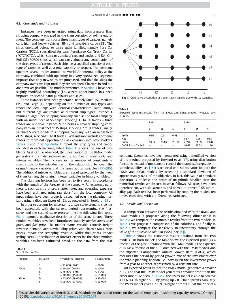
Fig. 1. Qualitative description of a two-stage scenario tree with six scenarios.

Table 2Expected economic results from the RMax and PMax models. Averages over10 runs.

RMax PMax

L M S L M S

Profit 0.93 0.91 0.91 1 1 1AIRR 1 1 1 0.87 0.88 0.88CAGR 24.1% 23.8% 23.3% 21.9% 21.8% 21.4%CAGR Extra Capital – – – 10.4% 12.2% 11.9%


4.1. Case study and instances

Instances have been generated using data from a major linershipping company engaged in the transportation of rolling equip-ment. The company transports three main types of cargoes, namelycars, high and heavy vehicles (HH) and breakbulk cargo (BB). Theships operated belong to three main families, namely Pure CarCarriers (PCCs), specialized for cars, Pure/Large Car Truck Carrier(PCTC/LCTCs), which can carry a mix of cars and trucks, and Roll On-Roll Off (RORO) ships which can carry almost any combination ofthe three types of cargoes. Each ship has a specified capacity of eachtype of cargo, as well as a total capacity to respect. The companyoperates several trades around the world. An internal policy at thecompany, combined with operating in a very specialized segment,imposes that only new ships are purchased, and that the ships thecompany owns are kept until they are scrapped. Charters in and outare however possible. The models presented in Section 3 have beenslightly modified accordingly (i.e., a zero-upper-bound has beenimposed on second-hand purchases and sales).

Three instances have been generated, namely Small (S), Medium(M), and Large (L), depending on the number of ship types andtrades included. Ships with identical characteristics (same family)but different age are treated as different ship types. Instance Lmimics a large liner shipping company such as the focal company,with an initial fleet of 55 ships, servicing 11 to 14 trades – threetrades are optional. Instance M describes a smaller shipping com-pany with an initial fleet of 35 ships, servicing 7 to 11 trades. Finally,instance S corresponds to a shipping company with an initial fleetof 27 ships, servicing 5 to 8 trades. Each instance includes optionaltrades to represent opportunities of expansion into new markets.Tables 6 and 7 in Appendix C report the ship types and tradesincluded in each instance, while Table 1 reports the size of pro-blems. As it can be observed, the linearization of the RMax modelgenerates a dramatic increase in the number of constraints andinteger variables. The increase in the number of constraints ismainly due to the introduction of the relationship between theoriginal binary variables and the linearization variables (75)–(90).The additional integer variables are instead generated by the needof transforming the original integer variables in binary variables.

The planning horizon has been set to five years, in accordancewith the length of the forecast at the company. All economic para-meters, such as ship prices, charter rates, and operating expenseshave been estimated using raw data from the focal company. Allinput values have been properly discounted over the planning hor-izon, using a discount factor of 12%, as suggested in Stopford [38].

In order to account for uncertainty a two-stage scenario tree hasbeen generated, with the current period representing the first-stage, and the second-stage representing the following five years.Fig. 1 reports a qualitative description of the scenario tree. Threerandom variables have been introduced, namely, market status, steelprice, and fuel price. The market status variable controls freightrevenue, demand, and newbuilding prices, and charter rates. Steelprices impact the scrapping revenue, whilst fuel prices impactsailing costs. A distribution of forecast errors for the three randomvariables has been estimated based on the data from the case

Table 1Size of the problems.

Problem Instance # Variables (Integer) # Constraints

S E18 000 (1200) E3000PMax M E40 000 (1600) E4000

L E75 000 (1 800) E5 000S E30 000 (15 000) E65 000

RMax M E55 000 (19 000) E80 000L E95 000 (23 000) E95 000


company. Scenarios have been generated using a modified versionof the method proposed by Høyland et al. [17], using distributionfunctions instead of moments to control the margins. Acceptable in-sample stability (see [18]) is achieved with six scenarios for both thePMax and RMax models, by accepting a standard deviation ofapproximately 0.6% of the objective. In fact, this value of standarddeviation is at least one order of magnitude smaller than thenumerical results we discuss in what follows. All tests have beentherefore run with six scenarios and solved to proven 0.5% optim-ality gap. Each test has been performed by running the models tentimes, each time with a different scenario tree.

4.2. Results and discussion

A comparison between the results obtained with the RMax andPMax models is proposed along the following dimensions: inTable 2 we compare the economic results from the two models, inTable 3 we propose a comparison of the solutions, and finally inTable 4 we compare the sensitivity to uncertainty through thevalue of the stochastic solution (VSS) (see [5]).

Table 2 shows the economic results obtained from the twomodels. For both models the table shows the expected profit (as afraction of the profit obtained with the PMax model), the expectedAIRR (as a fraction of the AIRR obtained with the RMax model), andthe expected “Compounded Annual Growth Rate” (CAGR) whichmeasures the period-by-period growth rate of the investment overthe whole planning horizon, i.e., how much the investment growsfrom a year to another, represented by a constant rate.

An expected result is that the PMax model generates a smallerAIRR, and that the RMax model generates a smaller profit than theother model. As seen in Table 2, the RMax model is able to achievea 13.6–14.9% higher AIRR by giving up 7.0–9.0% of profits. Similarly,the PMax model gives a 7.5–9.9% higher profits but at the price of a





Table 3Solutions to the RMax and PMax models. Averages over 10 runs.

Period (t) RMax PMax

L M S L M S

Newbuildings 0 6.7 3.6 2.6 19.4 8.6 5.9

1;‥; T �TL 12.1 6.4 4.4 11.9 8.5 5.6

Scrappings 0 – – – – – –

1;‥; T �1 12.9 8.1 5.6 10.8 7.3 5.2New trades 1 0.78 1.18 0.80 0.97 1.67 1.07

2 0.78 1.18 0.80 1.65 2.50 1.573 0.80 1.20 0.82 2.00 3.00 2.004 0.80 1.20 0.82 2.00 3.00 2.005 0.83 1.22 0.87 2.00 3.00 2.00

Table 4Value of the Stochastic Solution (VSS) for the RMax and PMax models. Averagesover 10 runs.

RMax PMax

L M S L M S

VSS (%) 11.9 15.9 21.7 12.6 3.3 11.7


12.0–13.0% smaller AIRR. The results are consistent over all theinstances representing companies of different sizes. The extraprofit gained with the PMax model is of course of value, but isgenerated by a higher employment of capital – Table 3 shows thehigher number of ships the PMax model suggests investing in. Inthis situation one may want to know whether it is sound toemploy that extra capital in order to gain extra profits.

Useful information in this sense may be found by looking at theCAGR generated by the two models (see Table 2). In both cases thecapital employed grows at a rate higher than 20%, with the RMaxmodel ensuring an approximately 2% higher growth. However, theCAGR generated by the extra capital employed in the PMax solutionis nearly halved compared to the capital employed in the RMaxsolution. This illustrates that the capital employed for extra profit isexpected to grow at a much slower rate. Whether to employ theextra capital for additional profits would depend on the presence ofother viable employment alternatives. Note, however, that thevalues of CAGR reported in Table 2 cannot be directly compared toactual CAGR values in the maritime industry. The values reportedhere do not take into account a number of additional expensesactually paid by real shipping companies, such as administrativecosts (insurance, cost of the administrative personnel) and taxation.We neglect such additional expenses, because (a) they would notplay any role in the optimization models presented as they areconstants, and (b) their precise estimate is made particularly diffi-cult due to the international set up of the focal shipping company.Therefore, we expect the values reported in Table 2 to be in generalhigher than historical market values and thus, only useful for acomparison in the scope of this paper.

Table 3 reports the solutions to both the RMax and PMaxmodels. The RMax model consistently (over the instances) sug-gests building much fewer ships in the first period than the PMaxmodel, and the same trend is to some extent maintained in thefollowing periods. The aggressive investment strategy suggestedby the PMax model is rarely seen in practice, and it can be dis-cussed whether it is realistic for a company to make investmentsof this size, compared to the initial value of the fleet. On the otherhand, the slow-paced newbuilding policy suggested by the RMaxmodel is more consistent with common practice in many shippingcompanies. Hence, the results of the RMax model could appearmore intuitive from a shipping company's perspective.


Furthermore, investing in as many ships as suggested by the PMaxsolution (e.g., 19 for the Large instance) raises doubts on whethercapital expenses and debt repayments can actually be afforded inday-to-day operations. Investments of this magnitude are rarelyseen in the industry. As an example, the focal shipping companytypically invests in less than a hand-full of ships every year. TheRMax formulation will only choose to invest in a new ship if theinvestment will lead to an equal or higher return than without theinvestment, which means that the extra profit gained over thecapital needed for the investment must be higher than the returnwithout the investment. If it is only marginally lower, the invest-ment will not be made. For the PMax model it is enough that theextra investment gives a net profit, as long as it is positive. So theRMax model can be said to have a stricter restriction on the profitan investment must generate.

As long as the scrapping policy is concerned, most of the shipsscrapped by the PMax model are the ones reaching the age limit.The RMax model instead suggests scrapping more of the youngership types in addition to the ones leaving the fleet. These resultsare consistent with the difference shown for the building policy. Infact, while the PMax model pursues a more aggressive capacityexpansion policy, the RMax model seeks renewal also for effi-ciency purposes. The average scrapping age suggested by theRMax model is close to the average scrapping age in the market(25 years) while the PMax model typically scraps ships when thereach the age limit imposed by the model (30 years).

The number of new trades entered by the PMax model is alsoconsistent with its new building and scrapping policy. Table 3shows that the expansion suggested by the PMax model is con-sistently choosing to service all optional trades but one. The tradenever chosen is characterized by a relatively low demand and highfrequency requirement. Again, the RMax model enters new mar-kets only if the corresponding remuneration increases the returnon the capital employment.

Table 4 reports the VSS for the two models. It can be noticedthat, except for the large instance, the VSS is higher for the RMaxmodel. It shows that planning against uncertainty has a muchhigher impact when maximizing the AIRR. The reason for thehigher VSS for the RMax model lays mainly in the smaller rate ofexpansion of the fleet. A smaller fleet is more vulnerable tochanges in demand as it offers fewer opportunities to increase thereturn by improving the management of the fleet. If the solution tothe mean value problem for the RMax model was used, it wouldgenerate a high amount of space charters to cater for peaks indemand. This is a symptom of tonnage deficit. On the opposite, themean value solution to the PMax model will suggest building abigger fleet (compared to the mean value solution to the RMaxmodel). Bigger fleets offer more flexibility when it comes torecovering from changes in demand. Therefore, returns are moreaffected by uncertainty than profits. This suggests that maximizingthe AIRR calls for planning against uncertainty, as plans made withaverage data are more subject to result in unbalanced fleets.

Finally, tests were run slightly modifying the instances intro-duced earlier in order to validate the results presented. For thesake of conciseness we just summarize our findings. Initially, wecompared the two models with an increased freight revenue(parameter RDits). The freight revenue obtained by the case com-pany was increased (possibly unrealistically) by up to 50%. Therationale behind this is that with a higher revenue for the cargoestransported, also the RMax model might find it profitable to investmore. However, the structural differences in the solutions shownin Table 3 were confirmed. The main difference is in the fact thatthe PMax model chooses to service all optional trades, and toinvest slightly more. However, for the RMax model the increasedrevenue was not sufficient to enter additional optional trades andexpand the fleet. Then, with respect to original instances, we






increased the number of optional trades (jNOt j ). Particularly, we

expanded instances S and M with two additional optional trades ineach. The higher number of optional trades pushed the RMaxmodel to increase the number of newbuildings. However, thisresult is ever more marked for the PMax model, stressing thestructural differences highlighted in the base case. A highernumber of optional trades makes the VSS drop for the PMaxmodel, confirming that the availability of more revenue options,together with a bigger fleet, offer decision makers more resiliencein case of poor fleet planning decision. The structural differencebetween the two models was also confirmed when considering alonger planning horizon, i.e., T ¼ 10. When decreasing the spacecharter cost (CSPkits), both models suggest investing in fewer ships(though the PMax model still suggests investing more than theRMax model). The option of sending cargoes by space charters isused more, and consequently fewer own ships are needed. Intui-tively, the VSS slightly decreases for both models, as space chartersrepresent in this case a rather cheap mean for recovering frompoor fleet planning decisions. Finally, we considered three stagesrather than two (i.e., we solved three-stage stochastic programsfor both models). The idea is that, in a two-stage structure, it mayhappen that investments are postponed until after the uncertaintyis disclosed. However, also with three-stages, the results shownwith the two-stage case are, to a very large extent, confirmed.

The adoption of the RMax in the maritime industry couldconfirm analytically the strategic ideas of shipping investors. Infact, as shown in this section, the solutions provided are to a largeextent compatible with common practices in the maritimeindustry. In addition, since the solutions to the RMax model arebalanced against an uncertain future, its adoption may help toprevent poor investment decisions merely caused by feelingsinduced by the raising or falling of shipping markets.

Table 5Notation.

SetsT Set of time periodsS Set of scenariosVt Set of ships available in the market in period t

VNt DVt Set of newbuildings which can be delivered in period t

Nt Set of all trades that the shipping company may operate in period t

NCt DNt Set of contractual trades

NOt DNt Set of optional trades

Lt Set of all loopsLvtDLt Set of loops which can be sailed by a ship of type v in period tLivtDLt Set of loops which include trade i and can be sailed by ship v in

period tK Set of all cargo types

VariablesyPvts Number of ships of type v in the fleet in period t, scenario sySCvts Number of ships of type v scrapped in period t, scenario syNBvts Number of ships of type v built in period t, scenario sySEvts Number of ships of type v sold in period t, scenario sySHvts Number of ships of type v bought in the second-hand market in

period t, scenario shIvts Number of ships of type v chartered-in for a period in period t,

scenario shOvts Number of ships of type v chartered-out for a period in period t,

scenario slUvts Number of ships of type v on lay-up for a period in period t, scenario

sxvlts Number of times loop l is sailed by ships of type v in period t,

scenario shSkits Amount of cargo of type k transported by space charters on trade i

in period t, scenario s

5. Conclusions

Strategic decisions related to capacity expansions or renewal,besides considering various operating constraints, may requireattention to a number of financial indicators, such as the AverageInternal Rate of Return (AIRR) besides or in addition to net presentvalues. In this paper we focused on the case of maritime shippingcapacity renewal. Shipping is a capital intensive industry whereuncertainty plays a major role. In addition shipping capacity ischaracterized by a long economic life. For these reasons, particularattention must be paid to the financial, in addition to the technical,fitness of investments in maritime shipping capacity.

We proposed a AIRR maximization model for the renewal ofmaritime shipping capacity, as well as a reformulation to eliminatethe nonlinear interaction between the decision variables. Themodel was compared with a more classic profit maximizationmodel, based on the available literature, on the case of a majorliner shipping company. The comparison shows that the profit lossincurred by the AIRR maximization model is smaller than the AIRRloss incurred by the profit maximization model, and that the extraprofit generated by the profit maximization model grows at aslower rate. Furthermore, we show that the profit maximizationmodel pursues an aggressive expansion policy, while the solutionsoffered by the AIRR maximization model are more consistent withcommon practice in the shipping industry, hence may betterrepresent the preferences of most shipping investors. Particularly,large publicly-traded shipping companies may find it moreappropriate to define strategies which maximize the return fortheir investors. However, none of the models is meant to be pre-ferable. As an example, small family-owned shipping companiesmay still find it reasonable to maximize profits. In any case, theAIRR maximization model extends the available literature offering


companies also the possibility to select capital employment deci-sions which maximize their return.

Several extensions or complementary analyses could be set upin future research efforts. The choice between profit or return as ametric could be facilitated by a multi-objective model whichconsiders the two objectives. Such a model would provide a Paretofrontier illustrating the trade-offs between the metrics involved,leaving the user decide what combination of them fits better thescope of the company. However, such model would pose addi-tional non-trivial challenges. In an attempt to maximize theweighed sum of the objectives, the way the two objected shouldbe normalized is far from obvious, given the magnitude differencebetween AIRR and profit, and the high number of variablesinvolved in the model. In addition, evaluating Pareto solutionswithout some assistance from the shipping industry is not trivial.It would be highly beneficial to receive inputs from the industry onwhat different combinations of profit and AIRR would mean inpractice. Related to this, a potential research avenue is a game-theoretical analysis of the industry, under the assumptions thatprofits or returns (or a combination of them) were maximized.This would shed light on how the adoption of such analytical toolwould impact the whole industry.

Acknowledgments

We thank the three anonymous reviewers for their insightfulcomments which helped improving the paper. This research ispartly funded by the GREENSHIPRISK and MARFLIX projects withfinancial support from the Research Council of Norway.

Appendix A

See Table 5.





Table 5 (continued )

δits Binary variable indicating whether optional trade i is serviced or notin period t, scenario s

cEts Capital employed by the shipping company in period t, scenario s

ParametersT The last time period in the planning horizonps The probability of scenario sCNBvts The cost for building a new ship of type v in period t, scenario sTL The lead time between order placement and deliveryCSHvts The cost of a ship of type v in period t, scenario s, in the second-

hand marketRSEvts The revenue from selling a ship of type v in period t, scenario s, in

the second-hand marketRSCvts The revenue from scrapping a ship of type v in period t, scenario sRCOvts The revenue from chartering out for a period a ship of type v in

period t, scenario sCCIvts The cost for chartering in for one period a ship of type v in period

t, scenario sRFVvs The value of a ship of type v at the end of the planning horizon

under scenario sCOPvt The fixed operating expenses met for a ship of type v in period tRLUvt The fixed operating expenses saving obtained when a ship of type

v is laid-up in period tCTRvlts The cost of sailing one time loop l with ship type v, in period t,

scenario sRDits The revenue obtained when meeting the transportation demand

on trade i, in period t, scenario sCSPkits The cost incurred when delivering one unit of cargo k on space

charters on trade t, in time t, scenario sCE0 The value of the fleet at the beginning of the planning horizonβ The yearly depreciation of the fleetYvt

NB The number of ships of type v ordered before the beginning of theplanning horizon and delivered in period t

YIPv The initial number of ships of type v in the poolYSHvts The number ships of type v available in the second-hand market

in period t, scenario sYSEvts The number ships of type v the company can sell market in period

t, scenario sYSHts The maximum number of second-hand purchases the company is

willing to issue in period t, scenario sYSEts The maximum number of sales the company is willing to issue in

period t, scenario sHIvts The number of ships of type v which is possible to charter in for

the whole period t, scenario sHOvts The number of ships of type v which is possible to charter out for

the whole period t, scenario sHIts The total number of ships the company is willing to charter out in

period t, scenario sHOts The total number of ships the company is willing to charter out in

period t, scenario sQv The total capacity of ship type v

Qkv The capacity of cargo type k of ships of type v

Zlv The time necessary to complete a loop l with ships of type v

Zv The fraction of a time period a ship of type v is availableFit The minimum number of times trade i must be visited in period tDkits The amount of cargo type k that must be transported across trade

i in period t, scenario s


Appendix B. Linearized AIRR maximization model

The RMax model (2b)–(40) can be written in the followinglinear equivalent way, as explained in Section 3.4. Particularly, forour specific case we empirically estimated that U¼1 is a validupper bound on w for all instances:

maxΠ ¼XsAS

ps �Xt A T:

tr T � TL

XvAVN

t þ TL

XjA JNB

CNBvtsy

NBjvts

264 ð51aÞ


þXt A T:to T

XvAVt

�XjA JSH

CSHvtsy

SHjvtsþ

XjA JSE

RSEvtsy

SEjvtsþ

XjA JSC

RSCvtsy

SCjvts

0@

1A ð51bÞ

�Xt A T:t4 0

XvAVt

COPvt y

Pvtsþ

XlALvts

CTRvltsxvlts�RLU

vt lUvts

ð51cÞ

þRCOvtsh

Ovts�CCI

vtshIvts

�ð51dÞ

þXt A T:t4 0

XiANO

t

RDitsδ itsþ

Xt A T:t4 0

XiANC

t

RDitsw�

XkAK

CSPkitsh

Skits

!ð51eÞ

þXvAV

T

RFVvs y

PvT s

35 ð51fÞ

subject to:

cEts ¼

βCE0wþ P

vAVNt þ TL

PjA JNB

CNBv0sy

NBjv0s

þ PvAVt

PjA JSH

CSHv0sy

SHjv0s�

PjA JSE

RSEv0sy

SEjv0s�

PjA JSC

RSCv0sy

SCjv0s

!; t ¼ 0; sAS;

βcEt�1;sþP

vAVNt þ TL

PjA JNB

CNBvtsy

NBvts

þ PvAVt

ð PjA JSH

CSHvtsy

SHvts�

PjA JSE

RSEvtsy

SEvts�

PjA JSC

RSCvtsy

SCvtsÞ; 1r trT �TL; sAS;

βcEt�1;sþP

vAVt

ð PjA JSH

CSHvtsy

SHvts�

PjA JSE

RSEvtsy

SEvts�

PjA JSC

RSCvtsy

SCvtsÞ; T �TLotrT �1; sAS;

βcEt�1;s; t ¼ T ; sAS:

8>>>>>>>>>>>>>>>>>>>>>><>>>>>>>>>>>>>>>>>>>>>>:

ð52Þ

yPvts ¼ yP

v;t�1;sþXjA JSH

ySHj;v;t�1;s�

XjA JSE

ySEj;v;t�1;s�

XjA JSC

ySCj;v;t�1;s;

tAT⧹f0g; vAVt⧹VNt ; sAS; ð53Þ

yPvts ¼ YNB

vt w; tAT : toTL; vAVNt ; sAS; ð54Þ

yPvts ¼

XjA JNB

yNBj;v;t�TL ;s; tAT : tZTL; vAVN

t ; sAS; ð55Þ

yPv0s ¼ YIP

v w; vAV0⧹VN0 ; sAS; ð56Þ

yPvts ¼

XjA JSC

ySCjvts; tAT⧹f0g; vAVt⧹Vtþ1; sAS; ð57Þ

XjA JSH

ySHjvtsrYSH

vtsw; tAT⧹fT g; vAVt ; sAS; ð58Þ

XjA JSE

ySEjvtsrYSE

vtsw; tAT⧹fT g; vAVt ; sAS; ð59Þ

XvAVt

XjA JSH

ySHjvtsrYSH

ts w; tAT⧹fT g; sAS; ð60Þ

XvAVt

XjA JSE

ySEjvtsrYSE

ts w; tAT⧹fT g; sAS; ð61Þ

lUvts�h

Ivtsþh

OvtsryP

vts; tAT⧹f0g; vAVt ; sAS; ð62Þ

hIvtsrHI

vtsw; tAT⧹f0g; vAVt ; sAS; ð63Þ

hOvtsrHO

vtsw; tAT⧹f0g; vAVt ; sAS; ð64Þ






XvAVt

hIvtsrHI

tsw; tAT⧹f0g; sAS; ð65Þ

XvAVt

hOvtsrHO

tsw; tAT⧹f0g; sAS; ð66Þ

XvAVt

XlALivt

QkvxvltsþXkAK

hSkitsZDkitsw; tAT⧹f0g; iANC

t ; kAK; sAS;

ð67ÞXvAVt

XlALivt

QkvxvltsZDkitsδ its; tAT⧹f0g; iANOt ; kAK; sAS; ð68Þ

XvAVt

XlALivt

QvxvltsZXkAK

ðDkitsw�hSkitsÞ; tAT⧹f0g; iANC

t ; sAS; ð69Þ

XvAVt

XlALivt

QvxvltsZXkAK

Dkitsδ its; tAT⧹f0g; iANOt ; sAS; ð70Þ

XvAVt

XlALivt

xvltsZFitw; tAT⧹f0g; iANCt ; sAS; ð71Þ

XvAVt

XlALivt

xvltsZFitδ its; tAT⧹f0g; iANOt ; sAS; ð72Þ

XlALvt

ZlvxvltsrZvðyPvtsþh

Ivt�h

Ovt� l

UvtsÞ; tAT⧹f0g; vAVt ; sAS; ð73Þ

δ itsrδ i;tþ1;s; tAT⧹f0; T g; iANOt ; sAS: ð74Þ

Objective function (51a)–(51f) and constraints (52)–(74) provide areformulation of the objective function and constraints of theRMax model. In addition, the following constraints must be added:XtAT

XsAS

pscEts ¼ T þ1; ð75Þ

w�δ itsþδitsr1; tAT⧹f0g; iANOt ; sAS; ð76Þ

δ its�wr0; tAT⧹f0g; iANOt ; sAS; ð77Þ

δ its�δitsr0 tAT⧹f0g; iANOt ; sAS; ð78Þ

w�yNBjvtsþyNBjvtsr1; jAJNB; tAT : trT �TL; vAVN

tþTL ; sAS; ð79Þ

yNBjvts�wr0; jAJNB; tAT : trT �TL; vAVN

tþTL ; sAS; ð80Þ

yNBjvts�yNBjvtsr0 jAJNB; tAT : trT �TL; vAVN

tþTL ; sAS; ð81Þ

w�ySHjvtsþySHjvtsr1; jAJSH ; tAT⧹fT g; vAVt ; sAS; ð82Þ

ySHjvts�wr0; jAJSH ; tAT⧹fT g; vAVt ; sAS; ð83Þ

ySHjvts�ySHjvtsr0 jAJSH ; tAT⧹fT g; vAVt ; sAS; ð84Þ

w�ySEjvtsþySEjvtsr1; jAJSE; tAT⧹fT g; vAVt ; sAS; ð85Þ

ySEjvts�wr0; jAJSE; tAT⧹fT g; vAVt ; sAS; ð86Þ

ySEjvts�ySEjvtsr0 jAJSE; tAT⧹fT g; vAVt ; sAS; ð87Þ

w�ySCjvtsþySCjvtsr1; jAJSC; tAT⧹fT g; vAVt ; sAS; ð88Þ


ySCjvts�wr0; jAJSC; tAT⧹fT g; vAVt ; sAS; ð89Þ

ySCjvts�ySCjvtsr0 jA JSC; tAT⧹fT g; vAVt ; sAS: ð90Þ

Constraints (75) correspond to the relationship introduced by Eq.(41), while constraints (76)–(90) define the relationships betweenthe original binary variables and the linearization variables asexplained by Glover [13]:

yNBjvtsryNBj�1;v;t;s; jA JNB⧹f1g; tAT : trT �TL; vAVNtþTL ; sAS; ð91Þ

ySHjvtsrySHj�1;v;t;s; jA JSH⧹f1g; tAT⧹fT g; vAVt ; sAS; ð92Þ

ySEjvtsrySEj�1;v;t;s; jA JSE⧹f1g; tAT⧹fT g; vAVt ; sAS; ð93Þ

ySCjvtsrySCj�1;v;t;s; jA JSC⧹f1g; tAT⧹fT g; vAVt ; sAS: ð94Þ

Constraints (91)–(94) strengthen the formulation by reducingsymmetry.

Finally, the domain of the variables is defined in (95)–(112):

yNBjvtsAf0;1g; jA JNB; tAT : trT �TL; vAVNtþTL ; sAS; ð95Þ

ySCjvtsAf0;1g; jA JSC; tAT⧹fT g; vAVt ; sAS; ð96Þ

ySHjvtsAf0;1g; jA JSH ; tAT⧹fT g; vAVt ; sAS; ð97Þ

ySEjvtsAf0;1g; jA JSE; tAT⧹fT g; vAVt ; sAS; ð98Þ

yNBjvtsARþ ; jAJNB; tAT : trT �TL; vAVN

tþTL ; sAS; ð99Þ

ySCjvtsARþ ; jAJSC; tAT⧹fT g; vAVt ; sAS; ð100Þ

ySHjvtsARþ ; jAJSH; tAT⧹fT g; vAVt ; sAS; ð101Þ

ySEjvtsARþ ; jAJSE; tAT⧹fT g; vAVt ; sAS; ð102Þ

yPvtsARþ ; tAT; vAVt ; sAS; ð103Þ

lvtsARþ ; tAT⧹f0g; vAVt ; sAS; ð104Þ

hIvtsARþ ; tAT⧹f0g; vAVt ; sAS; ð105Þ

hOvtsARþ ; tAT⧹f0g; vAVt ; sAS; ð106Þ

xvltsARþ ; tAT⧹f0g; vAVt ; lALvt ; sAS; ð107Þ

hSkitsARþ ; kAK; tAT⧹f0g; iANC

t ; sAS; ð108Þ

cEtsARþ ; tAT; sAS; ð109Þ

δitsAf0;1g; tAT⧹f0g; iANOt ; sAS; ð110Þ

δ itsARþ ; tAT⧹f0g; iANOt ; sAS; ð111Þ

wARþ : ð112Þ

Appendix C. Ship types and trades in the instances

Tables 6 and 7 report the ship types and trades, respectively,used in the instances described in Section 4.





Table 6Ship types in the instances. A negative age means that the ship can be deliveredfrom year t ¼ �Age. 1 RT43 E9.1 m3.

Ship type Age Capacity [RT43] Service Ships in initial fleet

Car BB HH Speed (knots) L M S

PCC1 26 4975 300 2200 18.5 4 4 3PCC2 12 6800 300 2500 18.5 6 3 2PCTC1 9 6800 300 2500 19 8 4 3LCTC1 4 6000 1500 2000 19 10 5 5PCTC2 4 5450 900 2200 19 12 7 2PCTC3 14 6150 200 1800 19.6 7 3 3RORO1 28 4853 1500 3100 20.5 6 3 2RORO2 �1 5660 2200 4000 20.8 2 0 1LCTC2 0 6000 1500 2000 18.5 0 2 0RORO3 �2 5660 2200 4000 20.8 0 0 0LCTC3 �1 6000 1500 2000 18.5 0 0 0RORO4 �3 5660 2200 4000 20.8 0 0 0LCTC4 �2 6000 1500 2000 18.5 0 0 0LCTC5 �3 6000 1500 2000 18.5 0 0 0

Table 7Trades in the instances. Each trade can be both Contractual (C) or Optional (O) indifferent trades.

Trade Length[NM]

Demand [Units RT43] Frequency Role in instance

Car HH BB L M S

T1 13 500 435 213 77 047 5762 48 C C CT2 11 700 103 048 14 201 4476 0 C C CT3 7800 41 036 24 420 3404 0 C C CT4 7500 19 200 0 0 0 C C CT5 13 000 89 406 21 427 7425 24 C C CT6 6500 469 379 67 854 20 075 52 C C –

T7 14 500 35 331 66 607 36 845 0 C C –

T8 7800 98 000 29 240 2689 0 C O OT9 4900 119 397 44 121 2167 0 C O –

T10 9000 60 159 7401 1939 48 O O OT11 8400 24 818 10 434 3252 0 O O OT12 6500 14 0508 53 928 14 115 0 O – –

T13 15 021 266 855 55 474 16 776 0 C – –

T14 19 200 397 688 123 779 66 198 48 C – –


References

[1] Adkins R, Paxson D. Deterministic models for premature and postponedreplacement. Omega 2013;41:1008–19.

[2] Ahmed S, King A, Parija G. A multi-stage stochastic integer programmingapproach for capacity expansion under uncertainty. Journal of Global Opti-mization 2003;26:3–24.

[3] Alvarez JF, Tsilingiris P, Engebrethsen ES, Kakalis NMP. Robust fleet sizing anddeployment for industrial and independent bulk ocean shipping companies.INFOR:Information Systems and Operational Research 2011;49:93–107.

[4] Bean JC, Higle JL, Smith RL. Capacity expansion under stochastic demands.Operations Research 1992;40:S210–6.

[5] Birge JR. The value of the stochastic solution in stochastic linear programs withfixed recourse. Mathematical Programming 1982;24:314–25.

[6] Chand S, Sethi S. Planning horizon procedures for machine replacementmodels with several possible replacement alternatives. Naval ResearchLogistics Quarterly 1982;29:483–93.

[7] Chand S, McClurg T, Ward J. A model for parallel machine replacement withcapacity expansion. European Journal of Operational Research 2000;121:519–31.

[8] Charnes A, Cooper WW. Programming with linear fractional functionals. NavalResearch Logistics Quarterly 1962;9:181–6.


[9] Christiansen M, Fagerholt K, Ronen D, Nygreen B. Maritime transportation. In:Barnhart C, Laporte G, editors. Handbook in operations research and man-agement science. North-Holland, Amsterdam: Elsevier; 2007. p. 189–284.

[10] Cormier G, Gunn EA. Modelling and analysis for capacity expansion planningin warehousing. Journal of the Operational Research Society 1999;50:52–9.

[11] Fagerholt K, Christiansen M, Hvattum LM, Johnsen TAV, Vabø TJ. A decisionsupport methodology for strategic planning in maritime transportation.Omega 2010;38:465–74.

[12] Fong CO, Srinivasan V. The multiregion dynamic capacity expansion problem:an improved heuristic. Management Science 1986;32:1140–52.

[13] Glover F. Improved linear integer programming formulations of nonlinearinteger problems. Management Science 1975;22:455–60.

[14] Goldstein T, Ladany SP, Mehrez A. A discounted machine-replacement modelwith an expected future technological breakthrough. Naval Research Logistics1988;35:209–20.

[15] Hoff A, Andersson H, Christiansen M, Hasle G, Løkketangen A. Industrialaspects and literature survey: fleet composition and routing. Computers &Operations Research 2010;37:2041–61.

[16] Hopp WJ, Nair SK. Markovian deterioration and technological change. IIETransactions 1994;26:74–82.

[17] Høyland K, Kaut M, Wallace SW. A heuristic for moment-matching scenariogeneration. Computational Optimization and Applications 2003;24:169–85.

[18] Kaut M, Wallace SW. Evaluation of scenario-generation methods for stochasticprogramming. Pacific Journal of Optimization 2007;3:257–71.

[19] Kimms A. Stability measures for rolling schedules with applications to capa-city expansion planning, master production scheduling, and lot sizing. Omega1998;26:355–66.

[20] King AJ, Wallace SW. Modeling with stochastic programming. New York, NewYork: Springer; 2012.

[21] Lawrence SA. International sea transport: the years ahead. Lexington: Lex-ington Books; 1972.

[22] Li S, Tirupati D. Dynamic capacity expansion problem with multiple products:technology selection and timing of capacity additions. Operations Research1994;42:958–76.

[23] Liu J, Ahuja RK, Sahin G. Optimal network configuration and capacity expan-sion of railroads. Journal of the Operational Research Society 2008;59:911–20.

[24] Luss H. Operations research and capacity expansion problems: a survey.Operations Research 1982;30:907–47.

[25] Magni CA. Average internal rate of return and investment decisions: a newperspective. The Engineering Economist 2010;55:150–80.

[26] Magni CA. The internal rate of return approach and the AIRR paradigm: arefutation and a corroboration. The Engineering Economist 2013;58:73–111.

[27] Magni CA. Investment, financing and the role of ROA and WACC in valuecreation. European Journal of Operational Research 2015;244:855–66.

[28] Menezes MBC, Kim S, Huang R. Return-on-investment (ROI) criteria for net-work design. European Journal of Operational Research 2015;245:100–8.

[29] Nair SK, Hopp WJ. A model for equipment replacement due to technologicalobsolescence. European Journal of Operational Research 1992;63:207–21.

[30] Pantuso G, Fagerholt K, Hvattum LM. A survey on maritime fleet size and mixproblems. European Journal of Operational Research 2014;235:341–9.

[31] Pantuso G, Fagerholt K, Wallace SW. Uncertainty in fleet renewal: a case frommaritime transportation. Forthcoming in Transportation Science; 2016. http://dx.doi.org/10.1093/trsc.2014.0566.

[32] Pantuso G, Fagerholt K, Wallace SW. Which uncertainty is important in mul-tistage stochastic programmes? A case from maritime transportation. Forth-coming in IMA Journal of Management Mathematics; 2016. http://dx.doi.org/10.1093/imaman/dpu026.

[33] Rajagopalan S. Capacity expansion and equipment replacement: a unifiedapproach. Operations Research 1998;46:846–57.

[34] Rajagopalan S, Soteriou AC. Capacity acquisition and disposal with discretefacility sizes. Management Science 1994;40:903–17.

[35] Rajagopalan S, Singh MR, Morton TE. Capacity expansion and replacement ingrowing markets with uncertain technological breakthroughs. ManagementScience 1998;44:12–30.

[36] Schall LD, Sundem GL, Geijsbeek WR. Survey and analysis of capital budgetingmethods. Journal of Finance 1978;33:281–7.

[37] Sethi S, Chand S. Planning horizon procedures for machine replacementmodels. Management Science 1979;25:140–51.

[38] Stopford M. Maritime economics. New York: Routledge; 2009.[39] UNCTAD. Review of maritime transport, 2012. United Nations, New York and

Geneva; 2012.[40] van Ackere A, Haxholdt C, Larsen ER. Dynamic capacity adjustments with

reactive customers. Omega 2013;41:689–705.


http://refhub.elsevier.com/S0305-0483(16)30037-8/sbref1


































































































http://dx.doi.org/10.1093/trsc.2014.0566

http://dx.doi.org/10.1093/trsc.2014.0566

http://dx.doi.org/10.1093/imaman/dpu026

http://dx.doi.org/10.1093/imaman/dpu026
























Documents

Maximizing the rate of return on the capital employed in ...isidl.com/wp-content/uploads/2017/07/E4420-ISIDL.pdfMaximizing the rate of return on the capital employed in shipping capacity