Computational statistics 2009

Assume a particular model with unknown parameters.

Determine how the likelihood of a given event varies with model model parameters

Choose the parameter values that maximize the likelihood of the observed event

The basic idea

Computational statistics 2009

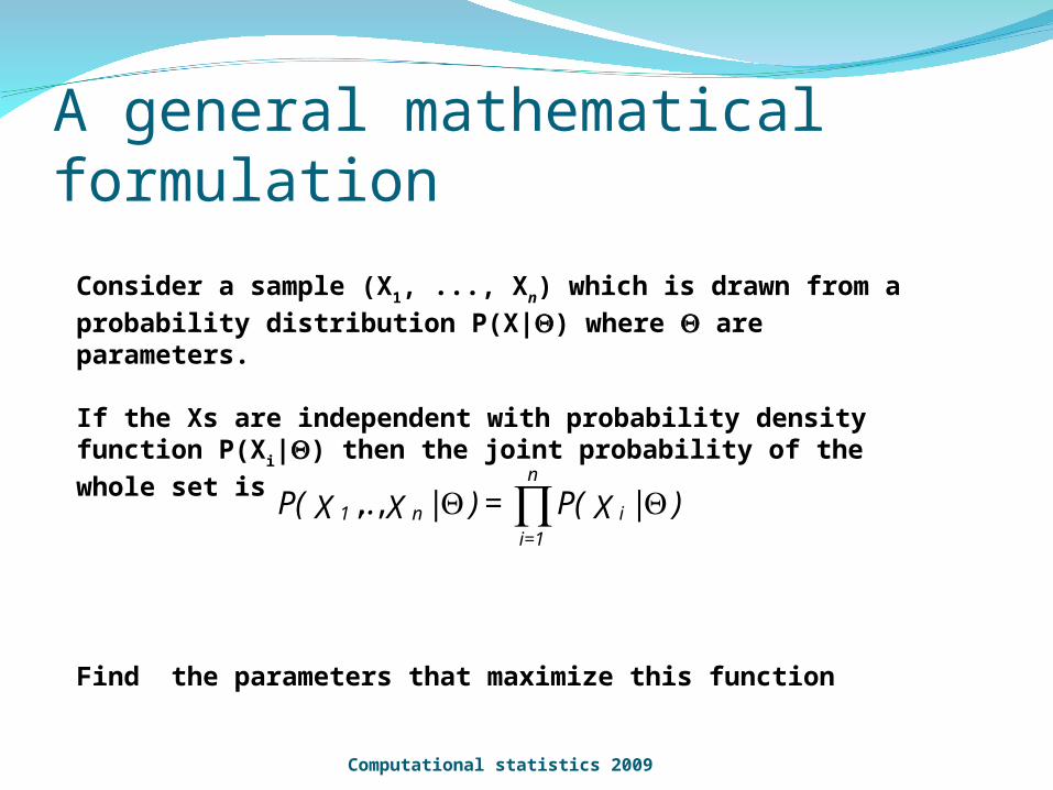
A general mathematical formulation

Computational statistics 2009

Consider a sample (X1, ..., Xn) which is drawn from a probability

distribution P(X|) where are parameters.

If the Xs are independent with probability density function P(Xi|)

then the joint probability of the whole set is

Find the parameters that maximize this function

 

)|XP(=)|X..XP( i

n

=1in1 ,,

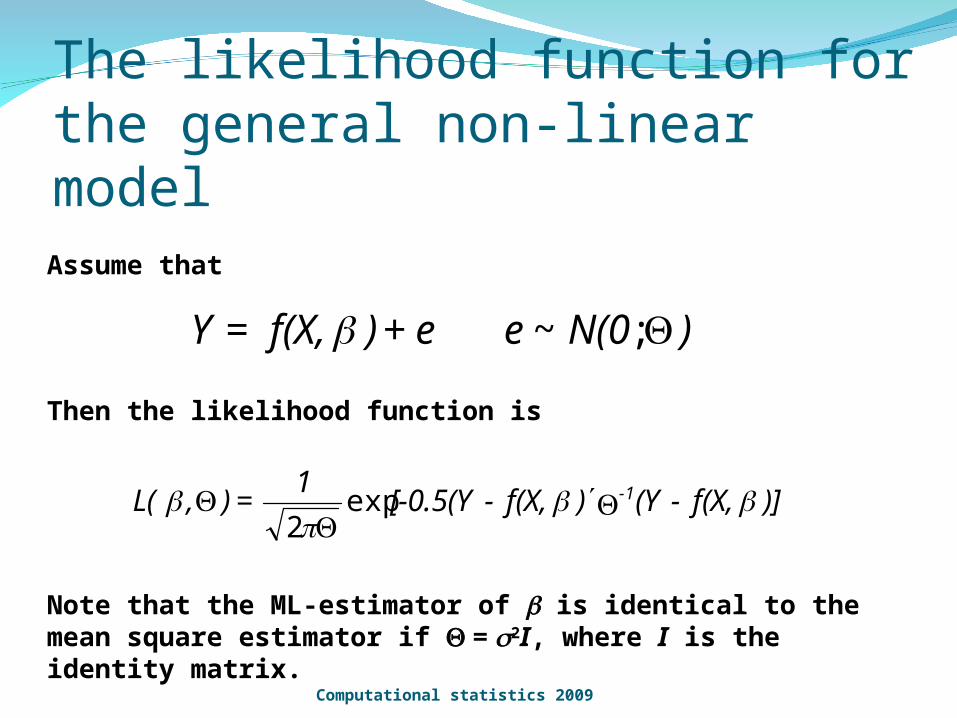
Assume that

Then the likelihood function is

Note that the ML-estimator of is identical to the mean square estimator if = 2I, where I is the identity matrix.

)]f(X,-(Y)f(X,-[-0.5(Y1

=),L( 1-

exp2

The likelihood function for the general non-linear model

Computational statistics 2009

)N(0e e+)f(X,=Y ;~

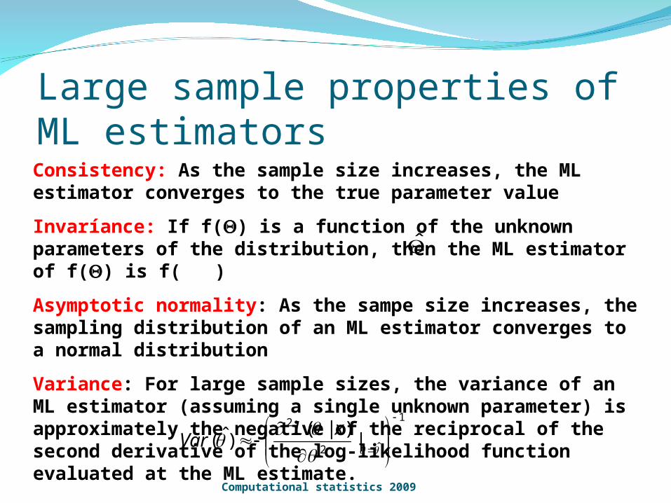
Consistency: As the sample size increases, the ML estimator converges to the true parameter value

Invaríance: If f() is a function of the unknown parameters of the distribution, then the ML estimator of f() is f( )

Asymptotic normality: As the sampe size increases, the sampling distribution of an ML estimator converges to a normal distribution

Variance: For large sample sizes, the variance of an ML estimator (assuming a single unknown parameter) is approximately the negative of the reciprocal of the second derivative of the log-likelihood function evaluated at the ML estimate.

Note that the ML-estimator of is identical to the mean square estimator if = 2I, where I is the identity matrix.

1

ˆ2

2

|)|(

)ˆ(

xLVar

Large sample properties of ML estimators

Computational statistics 2009

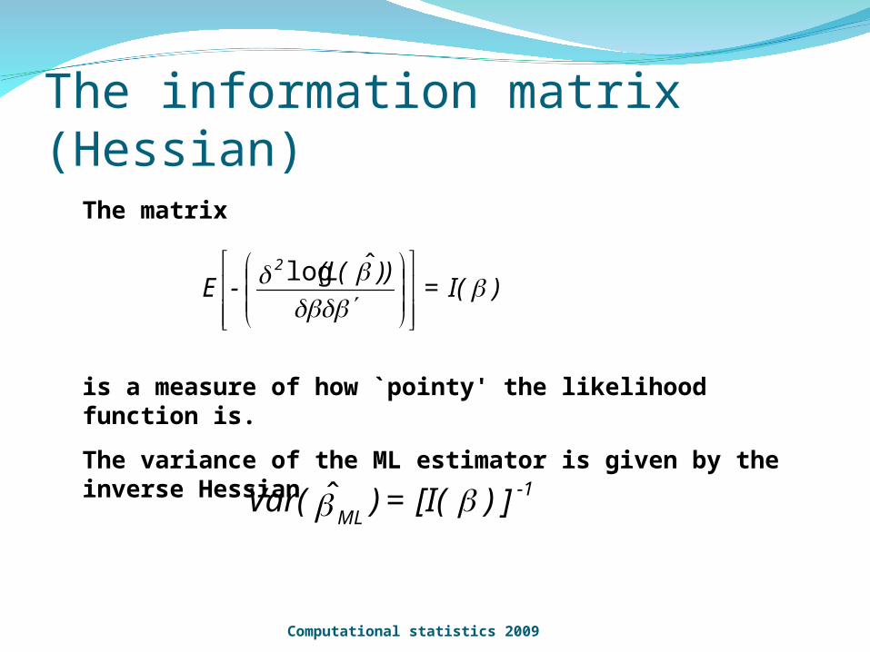
The matrix

is a measure of how `pointy' the likelihood function is.

The variance of the ML estimator is given by the inverse Hessian

)I(=))(L(

-E2

ˆlog

])[I(=)Var( -1

ML

The information matrix (Hessian)

Computational statistics 2009

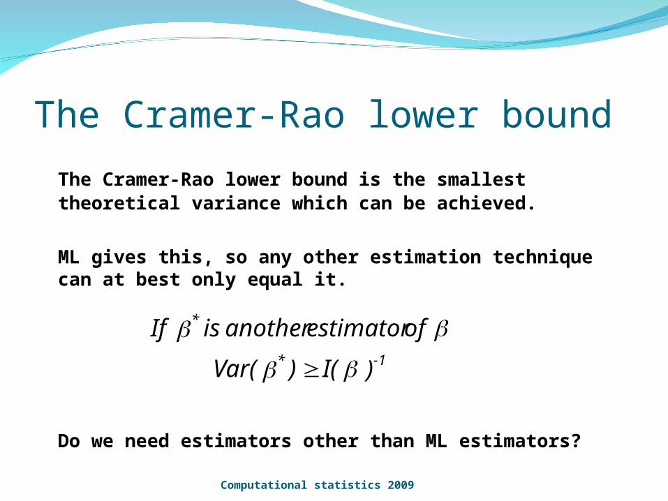
The Cramer-Rao lower bound is the smallest theoretical variance which can be achieved.

ML gives this, so any other estimation technique can at best only equal it.

Do we need estimators other than ML estimators?

)I()Var(

of estimator another is If1-*

*

The Cramer-Rao lower bound

Computational statistics 2009

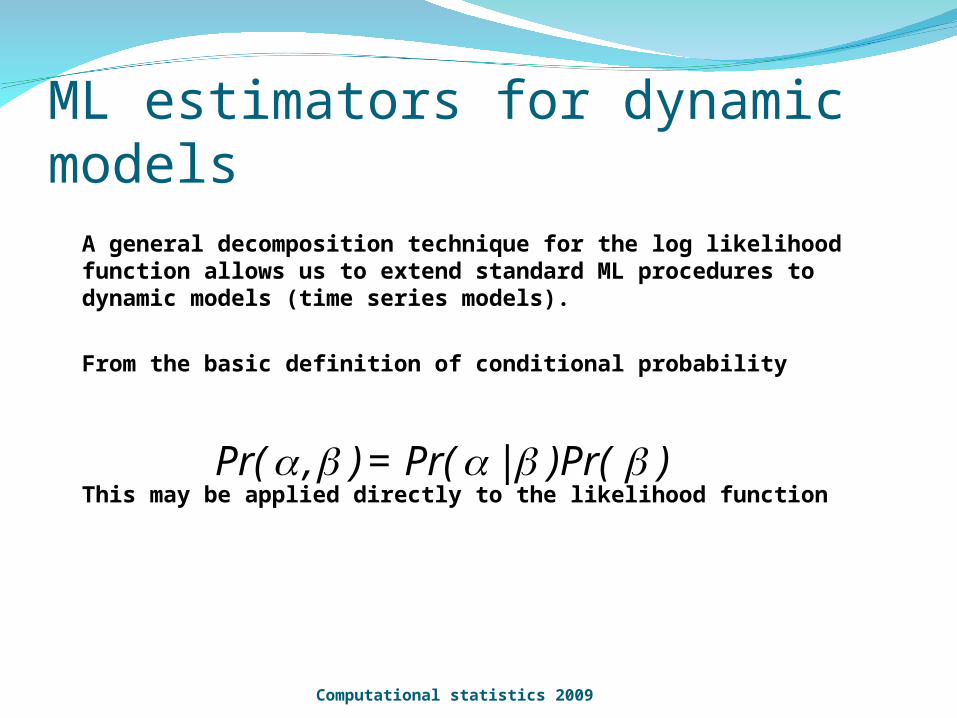
A general decomposition technique for the log likelihood function allows us to extend standard ML procedures to dynamic models (time series models).

From the basic definition of conditional probability

This may be applied directly to the likelihood function))Pr(|Pr(=),Pr(

ML estimators for dynamic models

Computational statistics 2009

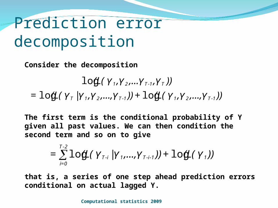
Consider the decomposition

The first term is the conditional probability of Y given all past values. We can then condition the second term and so on to give

that is, a series of one step ahead prediction errors conditional on actual lagged Y.

Prediction error decomposition

))Y,...,Y,Y(L(+))Y,...,Y,Y|Y(L(=

))Y,Y,...Y,Y(L(

1-T211-T21T

T1-T21

loglog

log

))Y(L(+))Y,...,Y|Y(L(= 11-i-T1i-T

2-T

0=i

loglog

Computational statistics 2009

Numerical optimization

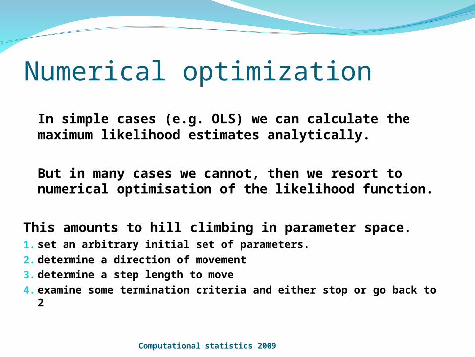
In simple cases (e.g. OLS) we can calculate the maximum likelihood estimates analytically.

But in many cases we cannot, then we resort to numerical optimisation of the likelihood function.

This amounts to hill climbing in parameter space. 1. set an arbitrary initial set of parameters.2. determine a direction of movement3. determine a step length to move4. examine some termination criteria and either stop or go back to 2

Computational statistics 2009

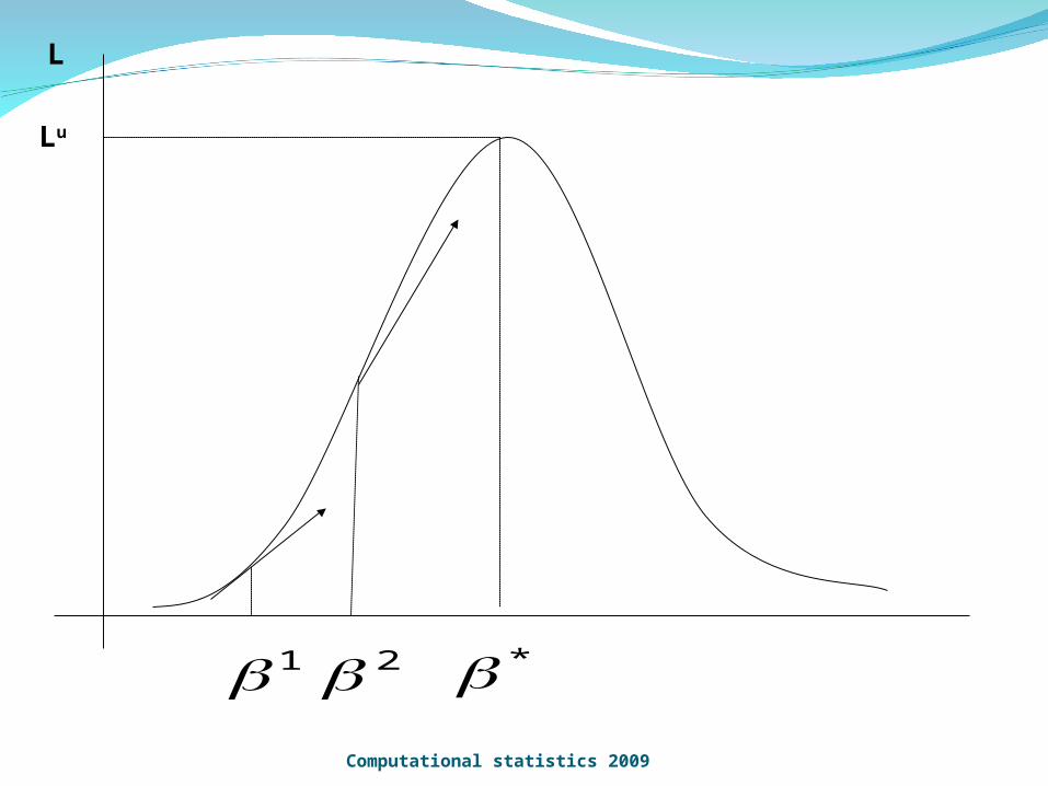
L

Lu

*1 2Computational statistics 2009

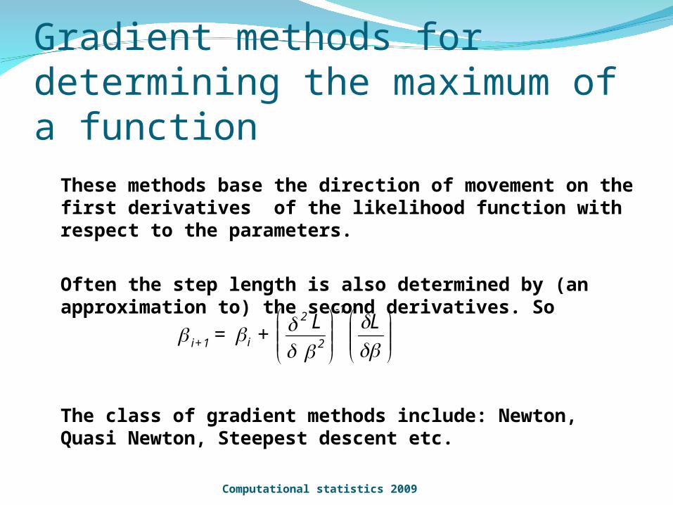
These methods base the direction of movement on the first derivatives of the likelihood function with respect to the parameters.

Often the step length is also determined by (an approximation to) the second derivatives. So

The class of gradient methods include: Newton, Quasi Newton, Steepest descent etc.

LL

+= 2

2-1

i1+i

Gradient methods for determining the maximum of a function

Computational statistics 2009

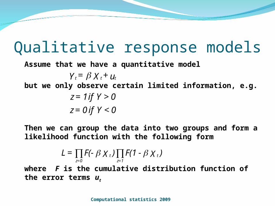
Assume that we have a quantitative model

but we only observe certain limited information, e.g.

Then we can group the data into two groups and form a likelihood function with the following form

where F is the cumulative distribution function of the error terms ut

u+X=Y ttt

0<Y if 0=z

0>Y if 1=z

Qualitative response models

Computational statistics 2009

)X-F(1)XF(-=L t1=z

t0=z