Embed Size (px)
Citation preview

MEAN-RISK PORTFOLIO OPTIMIZATIONPROBLEMS WITH RISK-ADJUSTED MEASURES
BY NAOMI LIORA MILLER
A dissertation submitted to the
Graduate School—New Brunswick
Rutgers, The State University of New Jersey
in partial fulfillment of the requirements
for the degree of
Doctor of Philosophy
Graduate Program in Operations Research
Written under the direction of
Andrzej Ruszczynski
and approved by
New Brunswick, New Jersey
October, 2008

c© 2008
Naomi Liora Miller
ALL RIGHTS RESERVED

ABSTRACT OF THE DISSERTATION
Mean-Risk Portfolio optimization problems with
risk-adjusted measures
by Naomi Liora Miller
Dissertation Director: Andrzej Ruszczynski
We consider the problem of optimizing a portfolio of finitely many assets whose
returns are described by a joint discrete distribution. We formulate the mean-risk
model, using as risk functions the semideviation and weighted deviation from quantile.
Using representation theorems from convex analysis, we write the portfolio problem
equivalently as a zero-sum matrix game, and provide convex optimization techniques
for its solution. A new set of risk-adjusted probability measures is derived from the
optimal saddle point solution of the game.
The risk-adjusted probability measures can be used to evaluate portfolio perfor-
mance. An illustrative example is provided in which these measures are derived for
a portfolio of 200 assets, and are used to evaluate a market portfolio and optimal
risk-averse portfolio. The results suggest the mean-risk portfolio is more robust than a
market portfolio.
We extend the above mean-risk model to the two-stage portfolio problem, where
there are two investment periods and the option to rebalance inbetween. The resulting
model is a two-stage stochastic programming problem, with mean-risk objectives in
ii

each stage. First and second stage risk-adjusted probability measures are derived in a
similar fashion to the one investment period problem.
Using as risk functions semideviation and weighted deviation from quantile in
both stages, we calculate the risk adjusted measures in a numerical example with 100
assets. These measures are used to evaluate a two-stage market portfolio and optimal
risk-averse portfolio.
We extend the cutting-plane and multi-cut algorithms for solving linear two-stage
stochastic problems to the two-stage mean-risk portfolio problem. The two-stage port-
folio problem is also formulated as one large linear program. We provide an illustrative
example, where a two-stage portfolio problem with risk functions semideviation and
weighted deviation from quantile is solved, using these two methods and the simplex
method. The performance of these three methods is compared for solving the portfolio
problem. On large examples, the extended cutting-plane and multi-cut plane algorithms
solve where the linear program fails.
iii

Acknowledgements
I came to Rutgers University in the fall of 2004 to pursue a Ph.D in Operations Research.
This was both an exciting and challenging time. Exciting as I was to expand my
knowledge and live away from home for the first time. Challenging as I was in a strange
place with almost no friends or family. The inevitable homesickness would creep in.
One of the few people I did know at the time, Al and Carol, would keep company on
the weekends and take me shopping when I didn’t have a car. Their friendship in the
first year was very helpful. I also acknowledge Ellen and Jerry Cohen, and Noam and
Michal, who invited me to Jewish seders.
I moved to a house on North Second Ave. in the late summer of 2005, where I met
my new roommates, Anupama Reddy and Rohan Fernandes. This was my first real
exposure to Indian cooking and movies. Their guidance through graduate school was
invaluable. Other people to mention in this regard include Lilya Fedzhora, Mine Subasi
and Vimla Gulabani.
It was in this second year of graduate school that I also began an indepedent research
study with my future advisor, Andrzej Ruszczynski. We began with the topic of risk-
adjusted bond valuation and ended up with the current topic of portfolio optimization
and risk-adjusted probability measures. I have enjoyed working with him these last
three years, and his guidance was invaluable.
I want to thank Dr. Eckstein for his helpful corrections and suggestions for the
dissertation draft.
Other friends in which I have spent much time and enjoyment with include Aritanan
Gruber, Minh Pham, Natalia Santa maria Tobar, Bjita Majumdar, Lilya Fedzhora and
Shilpa Shanbag.
The support of my family and friends from Toronto was invaluable. I mention
iv

here my parents, Harold Roy Miller, Jo-anne Miller, brother Jonathan Miller and Aunt
Shirley Miller. Also my very close friends Natalya Neman, Lee-Anne Wachtel and
Lindsay Shorser.
I make special mention of Rohan Fernandes, for his companionship and guidance
throughout graduate school.
v

Dedication
To my late grandparents, Isidore Jack Miller and Lily Miller
vi

Table of Contents
Abstract . . . . . . . . . . . . . . . . . . . . . . . . . . . . . . . . . . . . . . . . ii
Acknowledgements . . . . . . . . . . . . . . . . . . . . . . . . . . . . . . . . . iv
Dedication . . . . . . . . . . . . . . . . . . . . . . . . . . . . . . . . . . . . . . . vi
List of Tables . . . . . . . . . . . . . . . . . . . . . . . . . . . . . . . . . . . . . x
List of Figures . . . . . . . . . . . . . . . . . . . . . . . . . . . . . . . . . . . . xii
1. Preliminaries . . . . . . . . . . . . . . . . . . . . . . . . . . . . . . . . . . . 1
1.1. Introduction . . . . . . . . . . . . . . . . . . . . . . . . . . . . . . . . . . 1
1.2. The Portfolio Problem . . . . . . . . . . . . . . . . . . . . . . . . . . . . 3
1.3. Literature Survey . . . . . . . . . . . . . . . . . . . . . . . . . . . . . . . 5
2. The Abstract Risk-Averse Portfolio Problem . . . . . . . . . . . . . . 13
2.1. Formal Statement of the Risk-Averse Portfolio Problem . . . . . . . . . 13
2.2. Optimality and Duality Theory . . . . . . . . . . . . . . . . . . . . . . . 14
2.3. The Mean-Semideviation Model . . . . . . . . . . . . . . . . . . . . . . . 18
2.4. The Mean -Weighted Deviation from Quantile Model . . . . . . . . . . . 21
3. Numerical Experiments (Part 1) . . . . . . . . . . . . . . . . . . . . . . 25
3.1. Objective and Setup . . . . . . . . . . . . . . . . . . . . . . . . . . . . . 25
3.2. Results . . . . . . . . . . . . . . . . . . . . . . . . . . . . . . . . . . . . . 26
3.2.1. Mean-Semideviation Portfolio . . . . . . . . . . . . . . . . . . . . 26
3.2.2. Mean-Weighted Deviation From Quantile . . . . . . . . . . . . . 29
4. The Two- Stage Portfolio Problem . . . . . . . . . . . . . . . . . . . . . 33
vii

4.1. Formulation of the Standard Two-Stage Portfolio Problem . . . . . . . 33
4.2. Formulation of the Risk-Averse Two-Stage Portfolio Problem . . . . . . 37
4.3. The Time Consistency Property . . . . . . . . . . . . . . . . . . . . . . . 38
5. The Two-Stage Risk-Averse Portfolio Problem . . . . . . . . . . . . . 43
5.1. Optimality and Duality Theory . . . . . . . . . . . . . . . . . . . . . . . 43
5.2. The Mean-Semideviation Model . . . . . . . . . . . . . . . . . . . . . . . 45
5.2.1. Model Formulation . . . . . . . . . . . . . . . . . . . . . . . . . . 45
5.2.2. Subdifferentials . . . . . . . . . . . . . . . . . . . . . . . . . . . . 47
5.3. The Mean-Weighted Deviation from Quantile Model . . . . . . . . . . . 50
5.3.1. Model Formulation . . . . . . . . . . . . . . . . . . . . . . . . . . 50
5.3.2. Subdifferentials . . . . . . . . . . . . . . . . . . . . . . . . . . . . 51
6. Benders’ Decomposition . . . . . . . . . . . . . . . . . . . . . . . . . . . . 54
6.1. Review of Benders’ Decomposition . . . . . . . . . . . . . . . . . . . . . 54
6.2. Extension of Benders’ Decomposition . . . . . . . . . . . . . . . . . . . 59
6.3. Mean-Risk Models . . . . . . . . . . . . . . . . . . . . . . . . . . . . . . 62
6.4. Multi-Cut Benders’ Decomposition . . . . . . . . . . . . . . . . . . . . . 65
6.5. Multicut Risk Decomposition . . . . . . . . . . . . . . . . . . . . . . . . 65
6.6. Linear Model . . . . . . . . . . . . . . . . . . . . . . . . . . . . . . . . . 68
6.6.1. Semideviation . . . . . . . . . . . . . . . . . . . . . . . . . . . . . 68
6.6.2. Mean Weighted Deviation from Quantile . . . . . . . . . . . . . . 69
7. Numerical Experiments (Part 2 ) . . . . . . . . . . . . . . . . . . . . . . 71
7.1. Objectives . . . . . . . . . . . . . . . . . . . . . . . . . . . . . . . . . . . 71
7.2. Risk Aversion Parameter and Trading Costs . . . . . . . . . . . . . . . . 72
7.2.1. Risk Aversion Parameter . . . . . . . . . . . . . . . . . . . . . . 72
7.2.2. Trading Costs . . . . . . . . . . . . . . . . . . . . . . . . . . . . . 73
7.3. Optimal Portfolios and Risk-Adjusted Probability Measures . . . . . . . 76
7.3.1. Setup . . . . . . . . . . . . . . . . . . . . . . . . . . . . . . . . . 76
viii
7.3.2. Semideviation . . . . . . . . . . . . . . . . . . . . . . . . . . . . . 76
7.3.3. Mean-Weighted Deviation from Quantile . . . . . . . . . . . . . 79
7.4. Comparison of Different Solution Methods . . . . . . . . . . . . . . . . . 81
7.4.1. Setup . . . . . . . . . . . . . . . . . . . . . . . . . . . . . . . . . 81
7.4.2. Results on Solve Time . . . . . . . . . . . . . . . . . . . . . . . . 82
7.4.3. Results on Memory Usage . . . . . . . . . . . . . . . . . . . . . . 83
7.4.4. Results on Number of Iterations . . . . . . . . . . . . . . . . . . 86
7.5. Comparison of Aggregate and Conditional Risk Mapping Approach . . . 86
7.6. Progress of Benders’ Decomposition . . . . . . . . . . . . . . . . . . . . 89
8. Conclusion . . . . . . . . . . . . . . . . . . . . . . . . . . . . . . . . . . . . 90
References . . . . . . . . . . . . . . . . . . . . . . . . . . . . . . . . . . . . . . . 93
Vita . . . . . . . . . . . . . . . . . . . . . . . . . . . . . . . . . . . . . . . . . . . 96
ix

List of Tables
3.1. The mean-semideviation optimal portfolio . . . . . . . . . . . . . . . . 28
3.2. Risk-adjusted probability measures for the mean-semideviation optimal
portfolio . . . . . . . . . . . . . . . . . . . . . . . . . . . . . . . . . . . 28
3.3. The mean-deviation from quantile optimal portfolio . . . . . . . . . . . 30
3.4. Risk-adjusted probability measures for the mean-deviation from quantile
optimal portfolio . . . . . . . . . . . . . . . . . . . . . . . . . . . . . . . 31
7.1. The optimal two-stage mean-semideviation portfolio, Risk = −1.05478 77
7.2. First stage risk-adjusted probability measures for the optimal two-stage
mean-semideviation portfolio. . . . . . . . . . . . . . . . . . . . . . . . 77
7.3. The optimal two-stage mean-deviation from quantile portfolio, Risk =
−1.03599 . . . . . . . . . . . . . . . . . . . . . . . . . . . . . . . . . . . 79
7.4. First stage risk-adjusted probability measures for the optimal two-stage
mean-deviation from quantile portfolio. . . . . . . . . . . . . . . . . . . 80
7.5. Comparison of total solve time for two stage mean-semideviation port-
folio problem, using different solution methods. . . . . . . . . . . . . . 82
7.6. Comparison of total solve time for two stage mean-deviation from quan-
tile portfolio problem, using different solution methods. . . . . . . . . . 82
7.7. Comparison of total memory used by different solution methods, for the
two stage mean-semideviation portfolio problem. . . . . . . . . . . . . . 83
7.8. Comparison of ratios for memory usage, for different solution methods,
for two stage mean semideviation portfolio problem. . . . . . . . . . . . 84
7.9. Comparison of total memory used by different solution methods, for the
two stage mean-deviation from quantile portfolio problem. . . . . . . . 85
x

7.10. Comparison of ratios for memory usage, for different solution methods,
for the two stage mean deviation from quantile portfolio problem. . . . 85
7.11. The number of outer iterations generated in the master problem for
the two cutting plane methods, for the two-stage mean-semideviation
portfolio problem. . . . . . . . . . . . . . . . . . . . . . . . . . . . . . . 86
7.12. The number of outer iterations generated in the master problem for
the two cutting plane methods, for the two-stage mean-deviation from
quantile portfolio problem. . . . . . . . . . . . . . . . . . . . . . . . . . 86
7.13. Optimal portfolio for the two-stage mean-semideviation portfolio prob-
lem, with trading cost 0.005. Optimal objective value Risk = −1.05478
. . . . . . . . . . . . . . . . . . . . . . . . . . . . . . . . . . . . . . . . . 87
7.14. Optimal portfolio for the two-stage mean-semideviation portfolio prob-
lem, with trading cost 1. Optimal objective value Risk = −1.05331 . . 87
7.15. Optimal portfolio for the two-stage mean-deviation from quantile port-
folio problem, with trading cost 0.005. Optimal objective value, Risk
= −1.03599 . . . . . . . . . . . . . . . . . . . . . . . . . . . . . . . . . . 88
7.16. Optimal portfolio for the two-stage mean-deviation from quantile
portfolio problem, with trading cost 1. Optimal objective value Risk
= −1.03079 . . . . . . . . . . . . . . . . . . . . . . . . . . . . . . . . . . 88
xi

List of Figures
3.1. Cumulative distribution curves for the returns of the mean-semideviation opti-
mal portfolio. . . . . . . . . . . . . . . . . . . . . . . . . . . . . . . . . . . 29
3.2. Cumulative distribution curves of market portfolio for the semideviation risk
function. . . . . . . . . . . . . . . . . . . . . . . . . . . . . . . . . . . . . 29
3.3. Cumulative distribution curves of the market portfolio for the deviation from
quantile risk function. . . . . . . . . . . . . . . . . . . . . . . . . . . . . . 32
3.4. Cumulative distribution curves for the returns of the mean-deviation from quan-
tile optimal portfolio. . . . . . . . . . . . . . . . . . . . . . . . . . . . . . . 32
4.1. Scenario tree. . . . . . . . . . . . . . . . . . . . . . . . . . . . . . . . . . 34
7.1. Cumulative distribution curves of the mean-semideviation optimal portfolio, for
different values of the risk aversion parameter γ. . . . . . . . . . . . . . . . . 73
7.2. Cumulative distribution curves of the mean-deviation from quantile optimal
portfolio, for different values of the risk aversion parameter γ. . . . . . . . . . 74
7.3. Comparison of cumulative probability distribution curves for different trading
costs κ, for the semideviation risk function. . . . . . . . . . . . . . . . . . . 75
7.4. Comparison of cumulative probability distribution curves for different trading
costs κ, for the mean weighted devation from quantile risk function. . . . . . . 75
7.5. Comparison of the risk-adjusted and original cumulative probability distribution
curves for the mean-semideviation optimal portfolio. . . . . . . . . . . . . . . 78
7.6. Comparison of the risk-adjusted and original cumulative probability distribution
curves for the market portfolio, using the semideviation function. . . . . . . . 78
7.7. Comparison of the risk-adjusted and original cumulative probability distribution
curves for the mean-deviation from quantile optimal portfolio. . . . . . . . . . 80
xii

7.8. Comparison of the risk-adjusted and original cumulative probability distribution
curves for the market portfolio, using the weighted mean-deviation from quantile
risk function. . . . . . . . . . . . . . . . . . . . . . . . . . . . . . . . . . . 81
7.9. Graph of optimality gap to outer iteration number, for Benders decomposition
method, applied to mean-semideviation two-stage portfolio problem. . . . . . 89
xiii

1
Chapter 1
Preliminaries
1.1 Introduction
The problem of optimizing a portfolio of finitely many assets is a central problem in
theoretical finance. Markowitz introduced the classical approach to this problem in his
seminal paper [18]. In it, he argued that the portfolio performance should be measured
in two distinct dimensions: the mean E[R] of the portfolio return R, and the risk r[R],
which measures the variation of the return. In the mean-risk approach, the objective
was to select from the universe of all portfolios those that are efficient: for a fixed
value of the mean, the risk is minimized, and for a fixed value of the risk, the mean is
maximized.
The mean-risk approach has many advantages: it allows a trade off analysis be-
tween mean and risk. Moreover, it allows one to formulate the portfolio problem as a
parametric optimization problem.
The question of what risk function to use in the mean-risk approach has been ex-
amined extensively in the literature. One important direction of research was initiated
by Artzner et al [2] in their paper “Coherent Risk Measures”. In it, they outlined a
set of mathematical properties that a meaningful risk measure ought to satisfy. It was
argued that these axioms reflect the interests of risk-averse investors. In another vein,
Ogryczak and Ruszczynski [22, 23, 24] used stochastic dominance relations to compare
portfolio returns. They identified several risk functions for which the optimal portfolio
returns are non-dominated in terms of the second order stochastic dominance relation.
Important examples include the semideviation and weighted deviations from quantile.
Another important area of research is the optimization of a portfolio over multiple

2
investment periods. In particular, what optimization models should be used, and when
or if to rebalance a portfolio. An important recent development in this area has been
the conditional risk mapping approach [37]. The idea is to develop a model in which
information from the previous investment period can be used in the decision for the
next investment period. In the conditional risk mapping approach, such information is
incorporated using a stochastic programming formulation.
In the first part of this dissertation, we examine the mean-risk portfolio problem for
coherent risk functionals. We begin with a formal description of the portfolio problem,
followed by a literature review. In chapter 2, we review the main representation the-
orem for coherent risk measures and show that several mean-risk objective functions
are coherent. This, in combination with the optimality and duality theorems for the
portfolio problem, allow the mean-risk portfolio problem to be written as a zero-sum
matrix game. In [21], it is proved that certain probability measures arise as part of
the optimal saddle point solution to the game. We call these measures risk-adjusted
probability measures. In chapter 2, convex optimization techniques are provided for
solving the mean-risk portfolio problem with coherent risk functions in the form of
semideviation and weighted deviation from quantile. Closed forms for the risk-adjusted
probability measures are constructed for the above mean-risk models in these sections.
In chapter 3, the mean-risk portfolio problems for risk measures mean-semideviation
and mean-weighted deviation from quantile are solved for a portfolio of 200 assets. The
risk-adjusted probability measures are constructed for these examples. A market port-
folio is also constructed in each case and compared to the optimal mean-risk portfolio.
In the second part of the dissertation, we examine two-stage portfolio problems.
We begin with a formal description of the two-stage portfolio problem in chapter 4.
We review the conditional risk mapping approach to two stage optimization problems
and develop the two-stage mean risk model from it. In chapter 4, we argue for the
use of the conditional risk mapping approach and introduce the property of time con-
sistency, which this method satisfies. In chapter 5, we extend optimality and duality
theory from the first section to composite coherent risk measures, and develop matrix

3
game representations for both first and second stage optimization problems. We derive
first and second stage risk adjusted probability measures as part of the optimal saddle
point solutions to these problems. For the risk functions defined as semideviation and
weighted deviation from quantile, we derive closed forms for the first and second stage
risk-adjusted probability measures.
In chapter 6, we review Benders’ decomposition method for solving a linear two stage
stochastic programming problem. This method is extended to the two-stage mean risk
model, in particular, for the risk measures semideviation and weighted deviation from
quantile. The multi-cut version of Benders’ decomposition is introduced and extended
in a similar manner. A large linear programming formulation of the two stage mean-
risk portfolio problems for the risk measures semideviation and weighted deviation from
quantile is given.
Using semideviation and weighted deviation from quantile as risk functions in both
stages, we calculate the risk adjusted measures in a numerical example with 100 assets.
These measures are used to evaluate a two-stage market portfolio and optimal risk-
averse portfolio. In chapter 7, we solve a two-stage portfolio problem with risk functions
semideviation and weighted deviation from quantile, using these two methods and the
simplex method. The performance of these three methods is compared for solving
the portfolio problem. On large examples, the extended cutting-plane and multi-cut
algorithms solve where the linear program fails.
1.2 The Portfolio Problem
We begin with a formal description of the portfolio problem. Consider a collection of
n assets in which we would like to invest some intial capital C. For simplicity, we will
take C = 1. The n-dimensional vector R represents the collection of asset returns, with
each component Rj equal to the return of asset j, for j = 1..n. R is assumed to be an
integrable random variable on given probability space (Ω,F , P ), with R ∈ Ln1 (Ω,F , P ).
The vector z ∈ Rn represents our asset allocation, with each component zj equal to

4
the fraction of capital invested in asset j. The set Z of feasible portfolios is given below
Z = z ∈ Rn :∑n
j=1 zj ≤ 1, zj ≥ 0, j = 1..n.
In the analysis that follows, we will require only that Z is a convex, compact set
in Rn. So for example, one could limit the possible exposure of some assets by adding
additional upper bounds on the investments in asset j, or on groups of assets. All these
sets repesent closed convex sets in Rn, so can be used. The total return of the portfolio
at the end of the investment is RT z =∑n
j=1Rjzj .
The portfolio problem is to find an optimal way to invest the initial capital among the
n assets, in the face of uncertainty about the returns R. This is usually approached by
optimizing some objective function of the total return, over the set of feasible portfolios.
The general portfolio problem, with objective function ρ is given by
minz∈Z
ρ(RT z) (1.1)
We will examine the portfolio optimization problems where the objective function takes
the form
ρ(RT z) = −E[RT z] + γr[RT z]. (1.2)
This is the mean-risk approach introduced by Markowitz in his paper “Portfolio Selec-
tion” [18]. The term r[RT z] is a measure of the uncertainty of the portfolio return. In
his paper, Markowitz used the variance of returns as the risk measure. The non-negative
parameter γ represents our tolerance for risk. If γ = 0, then the problem reduces to
a standard problem of maximizing the mean, and we are more tolerant of risk. The
larger the value of γ, the more our tolerance for risk decreases. With this objective, we
define the mean-risk portfolio problem
minz∈Z−E[RT z] + γr[RT z]. (1.3)
There has been extensive research on what risk functionals r should be used in the
general mean-risk model. In the next section, we provide a more detailed interpretation
of the meaning of a risk functionals r, given in the literature, and what properties a
5
risk functional r should have. Examples of important risk functionals are given. We
use the term “risk functional ” for the part r[RT z] representing the uncertainty of the
return. The term “risk measure ” is used in the literature for the composite objective
of the form (1.2).
1.3 Literature Survey
The term risk plays a pervasive role in much of the literature on financial and economic
issues. Intuitively, it can be described as the chance of loss connected with a given
action [6]. There have been many attempts to define and characterize risk in the
literature, both for descriptive and prescriptive purposes. A detailed survey of these
attempts can be found in [6]. For the purposes of financial risk, we use the definition
of risk given in [41]. That is, risk is quantified on the basis of a random variable X.
In this context, risk is interpreted as the potential loss or profit of a position. It can
represent the future net worth of a portfolio, or the relative or absolute changes in an
investment.
A risk measure is defined in [41] as a mapping from the space of random variables
X representing outcomes to the real line.
Traditionally, the risk of a position was perceived as a dispersion in the values
of the corresponding random variable. Since Markowitz [18] and Tobin [44], it was
common to use the variance σ2 and standard deviation σ to measure the dispersion
of random variable X. The variance is defined as the average of the square of the
deviations from the mean, σ2 = E[ (X − E[X])2 ]. The standard deviation is defined
as the square root of the variance.
The variance and standard deviation have a number of nice properties. There are
well established statistical methods for estimating these measures from data [41]. In
particular, the mean-variance portfolio selection problem (1.3) can be reduced to a
parametric quadratic programming problem, for which there are standard solution
6
techniques.
An important criticism of the variance and standard deviation risk measures is that
they penalize overperformance equally to underperformance. When the random variable
X represents portfolio return, for example, returns above the mean are penalized. In
keeping with the idea that risk should be a measure of some “negative occurance ”, the
notion of downside risk measures was developed:
E[ max(c−X, 0)k ] (1.4)
The term c represents a target for which deviation below it is penalized. The number
k is a measure of the relative impact of the deviations. Important examples include
semideviation (c = E[X], k = 1) and semivariance (c = E[X], k = 2). Risk measures
of the form (1.4) were examined in [9] for a fixed target value of c. There has been
some disagreement over using a distribution-dependent target such as the mean for c.
It has been argued by [17, 7] that risk is frequently associated with the failure to obtain
a fixed target. To replace a set target c with a parameter (such as the mean) which
changes from distribution to distribution, is not favourable to this model.
A variation of the downside risk measure is to take
[ E[ max(c−X, 0)k ] ]1k (1.5)
Both (1.4) and (1.5) belong to one of the two larger classes of Stone’s risk measures
(see [42] for a description of these classes).
In more recent research, there has been a push to develop axiomatic models of
risk. Within this framework, there have been attempts to determine for which risk
functionals the mean-risk models of the portfolio problem (1.3) will be consistent with
these axioms. Two important axiomatic models are second-order stochastic dominance
theory (SSD) and coherence axioms. A review of both is provided and we discuss the

7
consistency of mean-risk models with these axioms.
Stochastic dominance [45] is based on an axiomatic model of risk-averse preferences
[9]. It has its origins in majorization theory [14] for the discrete case, and was later
extended to general distributions [13, 33]. It has been widely used in economics and
finance. In the stochastic dominance approach, the random variables are compared by a
pointwise comparison of some performance function, constructed from their distribution
functions. The first performance function of a random variable X is defined as the right
continuous cumulative distribution function
FX(η) = P (X ≤ η) ∀η ∈ R. (1.6)
The weak relation of first-degree stochastic dominance (FSD) is defined by
X FSD Y ⇔ FX(η) ≤ FY (η) ∀η ∈ R. (1.7)
The second-order performance function is given by areas below the distribution function
F
F 2X(η) =
∫ η
−∞FX(ξ)dξ, η ∈ R. (1.8)
A random variable X stochastically dominates random variable Y in the second order,
if F 2X(η) ≤ F 2
Y (η) for all η ∈ R. We write X SSD Y for second-order stochastic
dominance.
Strong FSD and SSD relations correspond to a strict inequality holding for at least
one η ∈ R. For decision making, the second order stochastic dominance relation is
most important. The SSD relation is consistent with risk-averse preference models
that prefer larger outcomes. A risk-averse investor’s preferences can be described by a
concave nondecreasing utility function u : R→ R. If X SSD Y , then we have
E[u(X)] ≥ E[u(Y )], (1.9)

8
for all non-decreasing concave utility functions u. Thus a risk-averse investor would
prefer position X over Y .
The consistency of mean-risk models with the second-order stochastic dominance
relation has been examined in [9, 22, 23, 24, 25]. A mean-risk model is SSD-consistent
if there exists a constant γ such that for all X,Y
X SSD Y ⇒
E[X] ≥ E[Y ] and E[X]− γr(X) ≥ E[Y ]− γr(Y )
In [25], the mean-risk model with the risk functional defined as semivariance
(corresponding to k = 2 in (1.4) ) was found to be SSD-consistent, but the constant γ
depends on the problem instance. This result was generalized by [9] to all mean-risk
models with risk functionals of the form (1.4) for which γ ≥ 1. In [22], the mean-risk
model with r defined as the absolute semideviation (1.11) with γ = 1 is found to be
SSD consistent. The mean-risk model with risk defined as deviation from quantile
α with γ = 1 is also found to be SSD consistent. In [47], the mean-risk model with
Gini’s mean absolute difference was found to be SSD-consistent. In the case of discrete
random returns, the mean-risk models can be formulated as linear programming
problems, and the mean-risk efficient frontier calculated using fast parametric simplex
method.
The coherence axioms are a more recent development, introduced in 1999 by Artzner
et al in [2]. Denote by X the space of all uncertain outcomes. In the context of the
portfolio problem, X = RT z and X = L1(Ω, F, P ).
Definition 1. A coherent measure of risk is a functional ρ : X → R which satisfies
the following four axioms:
A1 Convexity : ρ(αX + (1− α)Y ) ≤ αρ(X) + (1− α)ρ(Y ), ∀X,Y ∈ Z and α ∈ [0, 1];
A2 Monotonicity : If X,Y ∈ X , and X(ω) ≤ Y (ω) for all ω ∈ Ω, then ρ(X) ≥ ρ(Y );
A3 Translation Property : If a ∈ R and X ∈ X , then ρ(X + a) = ρ(X)− a;
9
A4 Positive Homogeneity: If t ≥ 0 and X ∈ X , then ρ(tX) = tρ(X).
Important examples of coherent risk measures ρ are obtained from certain mean-risk
models of the form
ρ(X) = −E[X] + γr[X] (1.10)
with scalar parameter γ ≥ 0 and risk functional r : X → R representing the variability
of the return. In particular, we may set r[X] to be the semideviation measure of order
p ≥ 1
r[X] = E[ (E[X]−X)p+ ]1p (1.11)
or the weighted mean-deviation from quantile
rα[X] = minη∈R
E[ max(1− αα
(η −X), (X − η) ], α ∈ (0, 1). (1.12)
It is well known that the optimal η in the above problem is any α−quantile of X. In
both cases, when γ ∈ [0, 1], the resulting mean-risk model is coherent [35].
Coherent risk measures have a very important representation theorem. Under fairly
mild conditions, when X represents final net worth, a coherent risk measure ρ can
be represented as the supremum of the expected negative value of X over a set A of
probability measures:
ρ(X) = supµ∈A
Eµ[−X]. (1.13)
The mean-risk models with the variance and standard deviation risk functionals are
not coherent [4]. Mean-risk models which are coherent include the mean-semideviation
and mean-deviation from quantile models [35]. The analysis of the construction of
quantile risk functionals is interesting in the context of coherent risk measures. We
provide a brief history of it. We begin with the VaR risk measure.
The value at risk measure (VaR), was introduced by JP Morgan Chase in 1994. At

10
a given probability level α ∈ (0, 1], and random variable X representing the loss of a
position, VaRα measures the minimum loss incurred in the α percent worst cases of a
portfolio. In [4], VaRα at probability level α ∈ (0, 1] is defined by
VaRα(X) = −xα (1.14)
where the upper quantile xα is defined as
xα = supx : P [X ≤ x] ≤ α. (1.15)
VaR concentrates on the upper tail of the loss distribution. It is useful to risk managers
concerned with the frequency of a default or probability of a loss, and not neccesarily
its size. It is used by financial institutions to determine how much capital to put aside
to control risk exposure [5] and how much capital is required for backing up trading
activities. An important property that VaR satisfies is the Law Invariance. It is given
in [41]:
Law Invariance : If P [X ≤ t] = P [Y ≤ t] ∀t ∈ R, then ρ[X] = ρ[Y ]; (1.16)
Law invariance states that if two random variables have identical distributions, then
the risk measure on those variables takes the same value. This is important in
industrial and financial applications, where VaR has to be estimated from empirical
data. An overview of different methods for estimating VaR is given in [8].
It turns out that VaR is not coherent. It satisfies the last three axioms, but
violates convexity. In [4], it is argued that violation of convexity is a serious flaw, as
it discourages portfolio diversification, an intuitive protection against risk. Rockafellar
and Uryasev [32] introduced a risk measure related to VaRα, which is both law
invariant and convex. The result was the expected shortfall, or the CVaR risk measure.
Expected shortfall at probability level α is the average loss in the worst 100α percent

11
cases [41, 4]. It is a measure of how much one can lose on average in states beyond
VaRα. The rigorous definition of ESα is given in [4] by
ESα[X] = − 1α
( E[X1X≤xα] − xα(P[X ≤ xα]− α) ). (1.17)
Here, 1A is the indicator function on the set A, defined by
1a =
1 if x ∈ A
0 if x 6= A
(1.18)
and xα is the upper quantile given in (1.15). The risk measure ESα is both law invariant
and coherent. There are more intuitive representations of ESα. If the generalized inverse
function of F (x) is introduced,
F−1(p) = infx|F (x) ≥ p) (1.19)
it was shown in [4] that ESα can be expressed as the negative mean of F−1(p) in the
interval [0, α].
ESα[X] = − 1α
∫ α
0F−1(p)dp. (1.20)
The authors in [24] argued that this formulation allowed for easier analysis of its prop-
erties. In [21] it is represented as
ESα(X) = −E[X] + rα[X] (1.21)
where rα[X] is the weighted mean-deviation from quantile risk measure. This represen-
tation is often referred to as the Average Value at Risk measure, or AVaR. The function
rα[X] is defined in [24], for X representing gain, by
rα[X] = minη∈R
E[max(1− αα
(η −X), (X − η)], α ∈ (0, 1). (1.22)
The expected shortfall risk measure ESα, or AVaRα, plays an important role in the

12
theory of law-invariant coherent risk measures. The following result is due to Kusuoka
[16] :
Theorem 2. If (Ω,F , P ) is nonatomic, for every lower semicontinuous law invariant
coherent measure of risk ρ[.] on L∞(Ω, F, P ), there exists a set N of probability measures
on [0, 1] such that
ρ[X] = supv∈N
∫ 1
0AVaRα[X]v(dα). (1.23)
Thus the expected shortfall risk measure is the building block for law-invariant
coherent risk measures. This result does not hold in general for the discrete case,
however, there are some classes of risk functionals for which Theorem 2 holds.
The measurement of risk of a position over many time periods is different from the
one-period risk measures discussed so far. In a portfolio problem, for example, with the
option to rebalance, information may become available at some interum time period.
In [37], the authors argue that this information may alter an investors perception of
risk from the previous investment period. They develop conditional risk mappings to
reflect this perception. The authors in [3] also discuss issues associated with information
becoming available during an investment period. The authors in [3, 29], and others,
have tried to develop axioms similar to the one-period coherence axioms (1).

13
Chapter 2
The Abstract Risk-Averse Portfolio Problem
2.1 Formal Statement of the Risk-Averse Portfolio Problem
In the next two sections, we formulate the abstract risk-averse portfolio optimization
problem. Optimality conditions and duality theory for the problem are provided and
important examples involving mean-risk models are given.
The portfolio problem was described in section (1.2). We review now the concept
of a risk measure and provide the space of outcomes on which it is defined. The
formulation of the abstract risk-averse portfolio problem follows that given in [35] and
specialized in [21].
An uncertain outcome is represented by a function X : Ω→ R. In what follows, X
represents the profit of a position. For example, X could be the return of a portfolio.
By a risk measure we mean a real-valued function ρ(X), defined on the set of uncertain
outcomes X . We use for X the space given in [35, 40],
X = Lp(Ω, F, P ), p ∈ [1,+∞). (2.1)
This space is important as many risk measures are defined in terms of p-th order
moments of a random variable. In the context of the portfolio problem, X = RT z
and X = L1(Ω, F, P ). We will assume that the risk measures ρ are proper, that is,
ρ(X) > −∞ for all X ∈ X and that the domain
dom(ρ) := X ∈ X : ρ(X) < +∞ (2.2)

14
is non-empty. The abstract risk-averse portfolio problem, with coherent objective func-
tion ρ is given below
minz∈Z
ρ(RT z) (2.3)
We observe that the function is convex and finite-valued on Rn. It is therefore
continuous [35]. As the set Z is compact, the minimum of ρ(RT z) is attained in Z,
and the problem has an optimal solution.
2.2 Optimality and Duality Theory
In order to develop optimality conditions for problem (2.3), we recall the representation
theorem of convex risk measures, first proved in [2] and then generalized in [10] and
[35]. The version here follows that given in [35].
As in the previous section, we let X be the space of F measurable functions with
finite pth order moment
X = Lp(Ω,F , P ), p ∈ [1,+∞). (2.4)
The dual space associated with X is the space X ∗ = Lq(Ω,F , P ) of linear functionals
on X , with q ∈ (1,∞], and 1p + 1
q = 1. The scalar product of X ∈ X and µ ∈ X ∗ is
defined as
〈µ,X〉 :=∫
Ωµ(ω)X(ω)dP (ω). (2.5)
The tuple (X ,X ∗, 〈·, ·〉) defines a paired topological space, and it is within this
framework that the main representation theorem for convex risk measures is presented.
In [30], the conjugate function ρ∗ : X ∗ → R of a convex risk function ρ : X → R is
ρ∗(µ) := supX∈X〈µ,X〉 − ρ(X) (2.6)

15
and the biconjugate function ρ∗∗ is
ρ∗∗(X) := supµ∈X ∗
〈µ,X〉 − ρ∗(µ). (2.7)
The Fenchel Moreau Theorem [30] states that if ρ is proper, convex and lower semicon-
tinuous, then ρ = ρ∗∗. That is,
ρ(X) = supµ∈X ∗
〈µ,X〉 − ρ∗(µ). (2.8)
It is proved in [30] that the conjugate function ρ∗ will be proper. Conversly, if (2.8)
holds for some proper function ρ∗ : Z∗ → R, then ρ is proper, convex and lower
semicontinuous. It is easily seen that (2.8) can be equivalently written as
ρ(X) = supµ∈U〈µ,X〉 − ρ∗(µ) (2.9)
where U = dom(ρ∗). If the risk measure in addition satifies one or more of the coherent
risk measure axioms, then more structure can be imposed on the set U , and a more
compact representation of ρ is possible. We use the representation theorem given in
[40].
Theorem 3. Suppose that ρ : X → R is convex, proper and lower semicontinuous.
Then representation (2.9) holds with U := dom(ρ∗). Moreover, we have that
1. Condition (A2) holds iff every µ ∈ U is non-positive, i.e. µ(ω) ≤ 0, ∀ ∈ Ω;
2. Condition (A3) holds iff∫
Ω µdP = −1 for every µ ∈ U ;
3. Condition (A4) holds iff the following representation holds
ρ(X) = supµ∈U〈µ,X〉. (2.10)
It follows that if ρ is a coherent risk measure, and is proper and lower-semi contin-
uous, then the representation
ρ(X) = supµ∈U〈µ,X〉 (2.11)

16
holds, with U being a subset of the following set
β := µ ∈ X ∗ :∫
Ωµ(ω)dP (ω) = −1, µ ≤ 0. (2.12)
Moreover, by positive homogeneity, the set U = ∂ρ(0). Thus the representation of co-
herent risk measures can be seen to follow naturally from the theory of convex functions.
We return to the portfolio problem. In this context, X = RT z and ρ(.) is a given
coherent risk measure. Suppose we define A = −U . We have by the representation
theorem that
ρ(RT z) = − infµ∈A〈µ,RT z〉 (2.13)
The mean-risk models with semideviations and deviations from quantile satisfy the
assumptions of the theorem and enjoy the representation (2.13). Owing to the theorem,
the portfolio optimization problem (2.3), with X = RT z and R ∈ Lp(Ω, F, P ) can be
written as an inf-max problem
−maxz∈Z
infµ∈A〈µ,RT z〉 (2.14)
If the risk measure ρ is continuous then the set A is bounded. As it is convex and
closed, it is weakly* compact. Therefore the ”inf” operation can be replaced by the
”min” operation. Moreover, due to the compacteness of Z and weak* compactness of
A, the ”min” and ”max” operations can be interchanged, and we can prove the main
optimality theorem [35].
Theorem 4. Suppose ρ is a continuous coherent measure of risk. A point z is an
optimal solution of problem (2.3) ⇔ ∃ a convex and weakly* closed set A ⊂ A such that
for all probability measures µ ∈ A the point z is also a solution of the problem
maxz∈Z〈µ,RT z〉. (2.15)

17
Furthermore, the set A is the set of solutions to the dual problem
minµ∈A
maxz∈Z〈µ,RT z〉. (2.16)
Proof. Let F (z, u) be the function defined on Z ×A as follows
F (z, µ) =∫
ΩRT (ω)zµ(ω)P (dω) (2.17)
The set Z is compact in Rn, and the set A is weakly compact in Lq. The function is
concave-convex and thus it has a saddle point (z, µ) on Z ×A :
F (z, µ) ≤ F (z, µ) ≤ F (z, µ), ∀z ∈ Z, ∀µ ∈ A. (2.18)
It follows that the optimal portfolio z optimizes the expected return with respect to
the optimal probability measure µ. We shall call µ the risk-adjusted probability mea-
sure. From the dual problem, it is seen that µ is the worst possible measure in the set A.
From now on, we assume the probability space Ω is finite, with m elementary
events ω1, ..., ωm occuring with probabilities p1, ..., pm. The vector p ∈ Rm denotes the
set of probabilities with coordinates pi, i = 1..m.
The matrix R will denote the possible asset returns: rji denotes the return of asset
j, in event i, where j = 1..n and i = 1...m. With this notation, Rp denotes the vector
of expected asset returns, RT z denotes the vector of portfolio returns, and pTRT z is
the expected portfolio return. The measure µ will be interpreted as a vector in Rm. In
this notation, the portfolio problem (2.3) can be written equivalently as
maxz∈Z
minµ∈A〈µ,RT z〉 (2.19)

18
with the dual problem
minµ∈A
maxz∈Z〈µ,RT z〉 (2.20)
This representation allows to view the portfolio problem as a matrix game, with
payoff matrix RT and strategies of players represented by the portfolio allocation z and
measure µ. Finding optimal asset allocation z and optimal risk-adjusted probability
measure µ is equivalent to finding a saddle point of the game, restricted to sets Z and
A. In the next two sections, we show several important mean-risk models that can be
formulated as linear programs in the discrete case, and we construct the risk adjusted
probability measure µ for these cases.
2.3 The Mean-Semideviation Model
The absolute semideviation risk measure r of a random variable X is defined as
σ[X] = Emax(E[X]−X, 0). (2.21)
The corresponding mean-risk model in this case takes the form
ρ[X] = −E[X] + γσ[X] (2.22)
It was proved in [22] that ρ(X) is consistent with second order stochastic dominance
for γ ∈ [0, 1]. In [35], it was proved that ρ(X) is coherent if γ ∈ [0, 1]. For discrete
distributions, we can identify X with a vector in Rn and write
ρ[X] = −〈p,X〉+ γm∑i=1
pi max(〈p,X〉 − xi, 0), (2.23)
where xi denotes the ith outcome of random variable X, and pi is its probability. The
portfolio problem, with X = RT z, becomes
minz∈Z−〈p,RT z〉+ γ
m∑i=1
pi max(〈p,RT z〉 − 〈ri, z〉, 0), (2.24)
19
where ri ∈ Rn represents the vector of asset returns corresponding to outcome i. Using
the representation theorem from the previous section, the portfolio problem can be
represented as
maxz∈Z
minµ∈A〈µ,RT z〉 (2.25)
with the dual problem
minµ∈A
maxz∈Z〈µ,RT z〉 (2.26)
Here A = −∂ρ(0) is a subset of the set of probability measures. The set A has been
described in [35]. In our notation, with discrete distributions, it takes the form
− ∂ρ(0) = µ : µ = (1− 〈g, 1〉)p+ g, 0 ≤ g ≤ γp (2.27)
The set A in this case can also be determined through the process of finding the convex
programming dual problem, as we now show.
Consider the portfolio problem given in (2.24). Denoting the shortfall[〈p,RT z〉−〈ri, z〉
]+
by si, we can write the problem as a convex programming problem
[21]:
Minimize − 〈p,RT z〉+ γ〈p, s〉
s.t. si ≥ 〈p,RT z〉 − 〈ri, z〉
s.t. s ≥ 0, z ∈ Z
(2.28)
Associate Lagrange multipliers ξ with the constraints in (2.28). The Lagrangian func-
tion is
L(z, s, ξ) = −〈p,RT z〉+ γ〈p, s〉+m∑i=1
ξi(〈p,RT z〉 − 〈ri, z〉 − si)
= (〈ξ, 1〉 − 1)〈p,RT z〉 − 〈ξ,RT z〉+ 〈γp− ξ, s〉

20
The dual function LD(ξ) is given by
LD(ξ) = infz∈Z,s≥0
L(z, s, ξ) (2.29)
By separating the term involving s from the terms involving RT z, the dual function
can be written as the sum of the optimal values of two problems:
LD(ξ) = minz∈Z(〈ξ, 1〉 − 1)〈p,RT z〉 − 〈ξ,RT z〉+ min
s≥0〈γp− ξ, s〉 (2.30)
Recall that the dual problem is defined by
maxξ≥0
LD(ξ) (2.31)
In order to simplify the presentation of (2.30), observe that LD(ξ) = −∞ unless the
following condition holds
γp ≥ ξ (2.32)
In this case, the dual function reduces to
LD(ξ) = minz∈Z〈(〈ξ, 1〉 − 1)p− ξ, RT z〉 (2.33)
Let A′ denote the set of elements
µ : µ = (1− 〈ξ, 1〉)p+ ξ, γp ≥ ξ, ξ ≥ 0 (2.34)
Then the dual problem becomes
maxµ∈A′
minz∈Z〈−µ,RT z〉 (2.35)
We show that µ is a probability measure. Note that 〈µ, 1〉 = 1. Moreover, due to
relation (2.32),
µ ≥ (1− γ〈p, 1〉)p+ ξ = (1− γ)p+ ξ ≥ 0 (2.36)

21
It follows that µ is a probability vector. By substituting ξ = γg, we observe that µ is
an element of the set A defined in (2.27). Thus there is a one-to-one correspondence
between the feasible points µ in the dual problem (2.35) and the elements of the set A
in (2.27).
It follows that the convex programming dual problem (2.35) coincides with the game
theoretic dual defined in (2.26). In this way, the following result has been proved.
Theorem 5. Suppose ρ(X) = −E(X) + γσ1(X) with γ ∈ [0, 1]. A vector z and a
measure µ constitute a saddle point of game (2.25) ⇔ the vector z is a solution of
problem (2.28) and
µ = (1− 〈ξ, 1〉)p+ ξ, (2.37)
where ξ are the Lagrange multipliers associated with constraints in (2.28).
It follows that we can obtain the risk adjusted probability measures by solving
the convex programming problem (2.28), obtaining the Lagrange multipliers ξ, and
applying the transformation in (2.37). When Z is a convex polyhedron, then linear
programming methods can be employed.
2.4 The Mean -Weighted Deviation from Quantile Model
Consider the weighted deviation from α-quantile risk measure defined in (2.39):
rα[X] = minη∈R
E
[max
(1− αα
(η −X), (X − η)) ]
, α ∈ (0, 1) (2.38)
The corresponding mean-risk model in this case takes the form
ρ[X] = −E[X] + γrα[X], (2.39)
It was proved in [22] that ρ(X) is consistent with second order stochastic dominance
for γ ∈ [0, 1]. In [35], it is proved that ρ(X) is coherent for γ ∈ [0, 1]. For discrete

22
distributions, we identify X with a vector in Rm and write
ρ[X] = −〈p,X〉+ γminη∈R
m∑i=1
pi max(
1− αα
(η − xi), xi − η). (2.40)
The portfolio problem, with X = RT z becomes
minz∈Z−〈p,RT z〉+ γmin
η∈R
m∑i=1
pi max(
1− αα
(η − (RT z)i), (RT z)i − η)
(2.41)
Using the representation theorem from the previous section, the portfolio problem
can be represented as
minz∈Z
maxµ∈A〈−µ,RT z〉 (2.42)
where A = −∂ρ(0) is a subset of the set of probability measures. The set A has been
described in [35]. In our notation, with discrete distributions, it takes the form
A = µ : µ = (1− γ)p+ γg, 0 ≤ gi ≤piα, i = 1..m, 〈g, 1〉 = 1. (2.43)
The set A in this case can also be determined through the process of finding the convex
programming dual problem, as in the previous section.
Consider the portfolio problem (2.41). Denoting by ui and vi the excess (xi − η)
and the shortfall (η−xi) respectively, the portfolio problem can be written as a convex
programming problem (see [21]):
Minimize − 〈p,RT z〉+ γm∑i=1
pi
(1− αα
vi + ui
)s.t. 〈ri, z〉 − η = ui − vi, i = 1, ..,m,
s.t. ui, vi ≥ 0, i = 1, ..,m,
s.t. η ∈ R, z ∈ Z
(2.44)
Here, ri denotes the return vector in the ith scenario. Associate Lagrange multipliers

23
ξi with the first set of constraints in (2.44). The Lagrangian function has the form
L(z, η, u, v, ξ) = −〈p,RT z〉+ γm∑i=1
pi(1− αα
vi + ui)
+m∑i=1
ξ(ui − vi − 〈ri, z〉+ η).
Collecting terms, we obtain
L(z, η, u, v, ξ) = −〈p+ ξ,RT z〉 − η〈ξ, 1〉
+ 〈γ(1− α)α
p− ξ, v〉+ 〈λp− ξ, u〉.
The dual function LD(ξ) is given by
LD(ξ) = infz∈Z,s≥0, η∈R, µ,v≥0
L(z, η, u, v, ξ). (2.45)
By separating the terms involving s, RT z and η, the dual function can be written as
LD(ξ) = minz∈Z−〈p+ξ,RT z〉−sup
η∈Rη〈ξ, 1〉+inf
v≥0γ
⟨1− αα
)p− ξ, v⟩
+infu≥0〈γp−ξ, u〉 (2.46)
The dual problem is given by
maxξ∈Rn
LD(ξ). (2.47)
In order to simplify the presentation of (2.46), observe that LD(ξ) = −∞ unless the
following conditions hold:
〈ξ, 1〉 = 0,
− γ(1− αα
)p ≤ ξ ≤ γp.
In this case, the dual function reduces to
minz∈Z〈−(p+ ξ), RT z〉). (2.48)

24
Let A′ denote the set of elements
µ : µ = p+ ξ, 〈ξ, 1〉 = 0 , −γ(1− αα
)p ≤ ξ ≤ γp , (2.49)
Then the dual problem becomes
maxµ∈A′
minz∈Z〈−µ,RT z〉. (2.50)
The conditions in A′ and γ ∈ [0, 1] imply that µ is a probability vector. We have that
〈µ, 1〉 = 〈p, 1〉+ 〈ξ, 1〉 = 1, since second term is 0. To check that µ is non-negative, note
that
µ = p+ ξ ≥ p+ γp = (1 + γ)p ≥ 0 (2.51)
By substituting ξ = γ(g − p), we observe that µ is an element of the set A defined in
(2.43). Thus there is a one-to-one correspondence between the feasible points ξ in the
dual problem (2.50) and the elements of the set A in (2.43).
It follows that the convex programming dual problem (2.48) coincides with the game
theoretic dual defined in (2.50). In this way, the following result has been proved.
Theorem 6. Suppose ρ(X) = −E[X]+γrα(X) with γ ∈ [0, 1]. A vector z and a vector
u constitute a saddle point of the game (9) ⇔ the vector z is a solution of problem
(2.41) and
µ = p+ ξ, (2.52)
where ξ are the Lagrange multipliers associated with problem (2.44).
It follows that we can obtain the risk adjusted probability measures by solving the
convex programming problem (2.41), obtaining the Lagrange multipliers ξ, and apply
the transformation in (2.52). When Z is a convex polyhedron, then linear programming
methods can be employed.

25
Chapter 3
Numerical Experiments (Part 1)
3.1 Objective and Setup
In this section, we find the optimal portfolios and compute the risk-adjusted probability
measures for the mean-risk portfolio optimization problems based on the semideviation
( problem (2.28)) and mean-deviation from quantile (problem(2.44)) measures of risk.
Each portfolio was drawn from a group of 200 assets taken from the S&P500 index.
Daily returns from the last 100 days of trading where taken as equally likely scenarios.
In each case, for risk aversion constant γ = 0.5, the cumulative distribution
functions(CDF) for the optimal portfolio returns were constructed: one using original
probability measures p, and the other using risk-adjusted probability measures µ.
These CDF’s were plotted against each other.
Separately, a market portfolio, with each asset having equal weight, was con-
structed. The CDF’s for both the original probability measures and the risk-adjusted
probability measures were constructed for this portfolio, and plotted against each other.
The shape of the cumulative distribution function provides a pictorial description
of the behaviour of the portfolio. For example, if the curve takes larger values at
negative returns, then the likelihood of poor portfolio perfomance is higher. So by
plotting the CDF’s for the original and risk-adjusted porbability measures, we are in a
sense comparing the perspectives on the behaviour of the portfolio.

26
Recall that the risk-adjusted probability measure represents the worst possible mea-
sure in the set A for the matrix representation of the portfolio problem
minz∈Z
maxµ∈A−〈µ,RT z〉. (3.1)
So a plot of the CDF of returns with respect to this risk-adjusted probability
measure would in some sense reflect for that portfolio the worst possible behaviour
for the returns. This is the curve used to reflect the perspective of a risk-averse investor.
If the CDF’s for both measures are close together, then the portfolio is in keeping
with the risk-averse investors’ preferences. If the curves are far apart, the optimal
portfolio does not reflect the concerns of a risk-averse investor. The former solution is
considered robust. By constructing and comparing the CDF’s for both the mean-risk
optimal portfolios and the market portfolios, we can determine if the former method
really does better reflect risk-averse investors preferences. The gaps in the former
should be smaller than in the latter if this is true. Our hypothesis is that this is true.
3.2 Results
3.2.1 Mean-Semideviation Portfolio
The optimal portfolio for the mean-semideviation portfolio problem is presented
in Table 3.1. In the table, the portfolio is heavily weighted towards three assets
(112, 138, 160), with the remaining capital dispersed more evenly among the other six
assets. As discussed earlier, the moderate size of the risk-penalty constant γ = 0.5
corresponds to a moderately diversified portfolio.
The risk-adjusted probability measures for the mean-semideviation portfolio prob-
lem are presented in Table 3.2. The CDF of returns with respect to these measures is

27
plotted against the CDF of returns with respect to the original probability measures
in Figure 3.1. In the figure, the risk-adjusted CDF has slightly higher probability
in the lower return values than the original CDF. This suggests a slightly more
pessimistic outlook on the part of a risk-averse investor. The curves are somewhat
close together, with a gap of value at most 0.1. This suggests a fairly robust portfolio.
This corresponds to the Table 3.2, were the risk adjusted probability measures are
fairly close in value to the original probability measures.
The risk-adjusted CDF is plotted against the original CDF in Figure 3.2 for the
market portfolio. In this figure, the curves are also fairly close together, suggesting in
this case, that even the market portfolio is somewhat robust.
So the hypothesis that the optimal portfolio is more robust than the market portfolio
is not really supported for the mean-semideviation portfolio problem, with γ = 0.5. For
larger γ coefficients, corresponding to a more risk-averse investor, the relationship may
change.

28
Asset Valuez15 0.035z33 0.061z73 0.016z99 0.037z112 0.34z138 0.12z160 0.30z164 0.04z178 0.05
Table 3.1: The mean-semideviation optimal portfolio
2 0.0077 21 0.0127 40 0.0127 59 0.0079 78 0.0127 97 0.01273 0.0127 22 0.0127 41 0.0127 60 0.0127 79 0.0127 98 0.00774 0.0077 23 0.0077 42 0.0127 61 0.0077 80 0.0127 99 0.00775 0.0077 24 0.0077 43 0.01207 62 0.0127 81 0.0077 100 0.00776 0.0077 25 0.0106 44 0.0127 63 0.0077 82 0.0127 101 0.01277 0.0077 26 0.0077 45 0.0077 64 0.0077 83 0.01198 0.0127 27 0.0127 46 0.0127 65 0.0127 84 0.01279 0.0077 28 0.0077 47 0.0077 66 0.0126 85 0.012710 0.0077 29 0.0127 48 0.0127 67 0.0077 86 0.009311 0.0127 30 0.0127 49 0.0127 68 0.0127 87 0.012712 0.0077 31 0.0127 50 0.0127 69 0.0077 88 0.012713 0.0077 32 0.0077 51 0.0127 70 0.0127 89 0.012714 0.0077 33 0.0077 52 0.0077 71 0.0127 90 0.007715 0.0127 34 0.0077 53 0.0127 72 0.0077 91 0.012716 0.0077 35 0.0077 54 0.0077 73 0.0077 92 0.012717 0.0127 36 0.0077 55 0.0077 74 0.0077 93 0.007718 0.0127 37 0.0077 56 0.0107 75 0.0077 94 0.007719 0.0077 38 0.0077 57 0.0077 76 0.0077 95 0.012720 0.0077 39 0.0077 58 0.0077 77 0.0077 96 0.0092
Table 3.2: Risk-adjusted probability measures for the mean-semideviation optimalportfolio

29
Figure 3.1: Cumulative distribution curves for the returns of the mean-semideviation optimalportfolio.
Figure 3.2: Cumulative distribution curves of market portfolio for the semideviation risk func-tion.
3.2.2 Mean-Weighted Deviation From Quantile
The optimal portfolio for the mean-weighted deviation from quantile portfolio problem
is presented in Table 7.3.
The risk-adjusted probability measures for the optimal mean-weighted deviation
from quantile portfolio problem are presented in Table 3.4. The risk-adjusted CDF is

30
plotted against the original-CDF in Figure 3.4 for the optimal portfolio. In the figure,
the curves are very close together. This suggests that the optimal portfolio is strongly
robust. This corresponds with Table 3.4, were the risk-adjusted probability measures
are close in value to the orignal probability measures.
The risk-adjusted CDF is plotted against the original-CDF in Figure 3.3 for the
market portfolio. In this figure, the curves diverge substantially. The risk-adjusted
measures predict a much more pessimistic outcome for the returns than the original
probability measures. This can be seen by the high value of the risk-adjusted CDF in
the negative half of returns, compared to the lower original CDF values in this interval.
The hypothesis that the optimal portfolio is more robust than the market portfolio
is strongly supported for the mean-weighted deviation from quantile portfolio problem.
The variation in the two curves can be explained by examining the risk functional. In
the weighted deviation from quantile risk functional, returns below the α-quantile are
penalized with coefficient 1−αα . For the five percent quantile, this coeeficient takes the
value 19, which is very high. For a market portfolio, with equally weighted assets, and
no effort to avoid this left tail, the penalty is applied with much higher frequency.
asset value asset value asset value asset valuez2 0.055 z5 0.062 z8 0.007 z9 0.011z12 0.007 z27 0.037 z30 0.023 z33 0.008z37 0.011 z42 0.010 z44 0.014 z46 0.019z58 0.066 z67 0.0542 z73 0.003 z84 0.005z94 0.030 z102 0.034 z104 0.015 z105 0.015z112 0.057 z119 0.102 z120 0.026 z127 0.004z133 0.068 z136 0.054 z138 0.026 z141 0.034z160 0.067 z177 0.005 z182 0.018 z184 0.018z191 0.026 z193 0.01
Table 3.3: The mean-deviation from quantile optimal portfolio

31
2 0.005 27 0.022 52 0.005 77 0.0053 0.005 28 0.018 53 0.050 78 0.0094 0.005 29 0.005 54 0.007 79 0.0175 0.005 30 0.005 55 0.005 80 0.0066 0.005 31 0.005 56 0.005 81 0.0057 0.010 32 0.005 57 0.005 82 0.0288 0.005 33 0.015 58 0.005 83 0.0059 0.005 34 0.005 59 0.005 84 0.00510 0.005 35 0.005 60 0.005 85 0.02811 0.005 36 0.005 61 0.005 86 0.00512 0.005 37 0.005 62 0.026 87 0.02313 0.005 38 0.005 63 0.005 88 0.00514 0.009 39 0.005 64 0.008 89 0.02115 0.042 40 0.005 65 0.019 90 0.00516 0.005 41 0.005 66 0.009 91 0.04817 0.02 42 0.011 67 0.005 92 0.04918 0.02 43 0.005 68 0.005 93 0.00519 0.005 44 0.005 69 0.005 94 0.00520 0.005 45 0.005 70 0.005 95 0.0121 0.005 46 0.005 71 0.011 96 0.00522 0.037 47 0.008 72 0.018 97 0.00723 0.005 48 0.005 73 0.005 98 0.00524 0.012 49 0.005 74 0.005 99 0.00725 0.018 50 0.005 75 0.005 100 0.00526 0.005 51 0.027 76 0.005 101 0.005
Table 3.4: Risk-adjusted probability measures for the mean-deviation from quantileoptimal portfolio
.

32
Figure 3.3: Cumulative distribution curves of the market portfolio for the deviation fromquantile risk function.
Figure 3.4: Cumulative distribution curves for the returns of the mean-deviation from quantileoptimal portfolio.

33
Chapter 4
The Two- Stage Portfolio Problem
4.1 Formulation of the Standard Two-Stage Portfolio Problem
In the first part of this dissertation, we introduced the risk-averse approach to opti-
mizing a portfolio of n assets over one investment time period. In this approach, we
formulated the following optimization problem
minz∈Z
ρ(RT z), (4.1)
where ρ was a coherent risk measure. The coherence of ρ allowed us to rewrite the
problem as a matrix game and to derive new risk-adjusted probability measures. The
risk-averse approach was argued to reflect the attitudes of a risk-averse investor.
In this section, our objective is to formulate an analogous risk-averse approach to
optimizing a portfolio over two time periods. In particular, we are interested in the
case where the option exists to rebalance the portfolio in between the two time periods.
With this in mind, we formulate the conditional risk mapping approach for optimizing
the portfolio and argue for its benefits. The resulting two-stage portfolio optimization
problem is called a two-stage risk-averse portfolio problem.
We begin with a review of the two-stage portfolio problem with rebalancing.
Consider a collection of n assets in which investment decisions are to be made in two
consecutive time periods. The return of the assets in each stage are assumed to be n
- dimensional integrable random variables, Rt on some probability space, with Rtj the
return of asset j in stage t, for t ∈ 1, 2.

34
Our asset allocations in the first and second stage are denoted by the n-dimensional
vectors zt, with components ztj representing the amount of capital invested in asset j
during stage t, for t ∈ 1, 2. The end portfolio value in stage t is given by (ξt)T zt,
where
ξt = 1 +Rt (4.2)
In the portfolio problem with rebalancing, the capital at the end of the first stage,
given by (ξ1)T z1 is reallocated among the assets, prior to observing the second stage
return outcomes.
In what follows, we consider the portfolio problem for the discrete case, where the
vector random variables ξ1 and ξ2 have a finite number of realizations. In this case, we
can visualize the possible sequence of outcomes ξ = (ξ1, ξ2) by a scenario tree
Figure 4.1: Scenario tree.
The nodes in level one and two represent the possible realizations of ξ1 and ξ2,
while the root node at level 0 represents the beginning of the process. Each node i in
level one is connected to a set of children nodes, Ci in level two, representing the
possible outcomes of ξ2 following the first stage outcome. The root node connects to

35
all nodes in level one, and a path from the root node to an end node represents a
sequence of possible outcomes for (ξ1, ξ2).
We can associate with the root node a probability vector p1 ∈ Rm1 , with p1i the
probability of outcome i occuring in the first stage. Similarly, we can associate with
each node i in the first level, the probability vector p2i ∈ Rm2 , with p2
il the probability
of moving to node l in level two from this node.
Note that z2 becomes an n × m1 matrix, with entry z2ji representing the second
stage asset allocation, given that outcome i occured in the first stage. We can formulate
explicitly the form of the sets Z2i for the case where the portfolio is rebalanced after
the first stage, subject to trading costs:
Z2i = z2i :
n∑j=1
ξ1j z
1j − κ
n∑j=1
|z2ji − ξ1
j z1j | ≥
n∑j=1
z2ji, z2
i ≥ 0, κ ∈ [0, 1] (4.3)
Here, the total trading costs are given by term κ∑n
j=1 |z2ji − ξ1
j z1j |. In the literature,
these are calculated for each asset j as a non-negative fraction of the amount traded.
The total amount invested in the second stage must not exceed the first stage end
portfolio minus the total trading costs. This is given by the main constraint in the set.
The two stage portfolio problem with rebalancing fits into the class of stochastic
programming problems with recourse, described in [27] and [40]. That is, we have a
decision problem over m time periods, m ≥ 2, where at least one decision is preceded
by an observation. The decision process for the two-stage problem can be represented
by the following diagram.
1. Decision z1 → 2. Observation ξ1
3. Decision z2 → 4. Observation ξ2
A standard approach described in [27] and [40] to solve this problem is to construct a
36
linear two-stage problem
Minimize cT z1 + E[Q(z1)]
s.t. Az1 = b, z1 ≥ 0(4.4)
where Qi(z1) is the optimal value of the ith second stage problem
Minimize qTi z2i
s.t. Tiz1 +Wiz2 = hi, z2
i ≥ 0(4.5)
In these formulations, some or all of the vectors in the 4-tuple (q,W, T, h) are random.
In many cases, the vector qi represents the conditional expectation of a random function,
−Ep2i [ξ2i ]. The first and second stage feasible sets are closed and convex in Rn. In the
case of the portfolio problem, we can replace the sets with Z1 and Z2i. The difficulty
arises that the set Z2i is not defined by an inequality involving a linear function. It
can be proved however that (4.5) has the same solution when Z2i is replaced by the
following convex set
Z2i = (z2i , ui, vi) :
n∑j=1
ξ1j z
1j − κ
n∑j=1
(uji + vji) ≥n∑j=1
z2ji
uji − vji = ξ1j z
1j − z2
ji, z2i ≥ 0 u ≥ 0, v ≥ 0 κ ∈ [0, 1]
(4.6)
With the set Z2i replaced by Z2i, the linear two-stage problem takes the form
minz1∈Z1
cT z1 + E[Q(z1)] (4.7)
with Qi(z1) is the optimal value of
minz2i ∈Z2i
cT2iz2i + (−Ep2i [ξ
2i ])T z2
i (4.8)
We can visualize the linear two-stage approach (4.7) - (4.8) by considering what
happens after observing ξ1. At this point, outcome i has occurred, and this is
represented by node i in the scenario tree. At node i, the optimization problem is to
maximize the expected value of the portfolio at the end of the second stage, where the

37
expectation is taken over the children nodes Ci. That is, the conditional expectation
of ξ2z2, given that we are at node i, must be optimized. The first stage problem is to
optimize the portfolio over all possible outcomes i.
4.2 Formulation of the Risk-Averse Two-Stage Portfolio Problem
The conditional risk mapping approach to portfolio optimization builds on this method.
That is, the decision-making for stage two is based on the restricted set of possible
outcomes given we are at node i. However, we may choose, instead of conditional
expectation, any coherent risk measure. For example, we may use conditional mean-
semideviation
ρ2i(Z) = −Ep2i [Z] + γiEp2imax((Z − Ep2i [Z]), 0), γi ∈ [0, 1] (4.9)
or conditional mean-deviation from quantile
ρ2i(Z) = −Ep2i [Z] + γiEp2imax(
1− αα
(Z − η), (η − Z)), γi ∈ (0, 1) (4.10)
Here, we set Z = ξ2i z
2i for notational convenience. Suppose we denote by Qi(z1) the
optimal solution to the optimization problem at node i.
Qi(z1) = minz2i ∈Z2i
cT2iz2i + ρ2i(ξ2
i z2i ) (4.11)
As in the standard stochastic programming approach, we optimize some composite
function ρ1 over all 2nd stage optimal solutions. That is, we formulate the first stage
problem
minz1∈Z1
cT z1 + ρ1(−Q(z1)) (4.12)
Here, ρ1 is a coherent risk measure, and Q(z1) is the random variable taking the value
Qi(z1) with probability p1i . We call problem (4.12) the risk-averse two-stage portfolio
optimization problem. If we choose ρ1 = −E[.], then we obtain model (4.4).

38
We provide briefly some explanantion for why the composition of ρ1 is taken with
respect to −Q(.). Recall the monotonicity condition
If X,Y ∈ Z, and X(ω) ≤ Y (ω) for all ω ∈ Ω, then ρ(X) ≥ ρ(Y )
We note that the risk measure ρ is actually negatively monotone. That is, ρ decreases
in value as X increases in value. Thus, if X = Q(.) represents a convex function, which
is non decreasing, then the composition φ = ρ(Q(.)) would result in a non-increasing
and concave function. As we are interested in coherent mean-risk models, we require
this composition to be nondecreasing and convex. Hence we take −Q(.). The following
proposition formalizes this argument [40]:
Proposition 7. Let X be an Lp space. If the mapping Q : Rn → X is convex and ρ :
X → R satisfies conditions (A1) and (A2), then the composite function φ(.) := ρ(−Q(.))
is convex.
4.3 The Time Consistency Property
Consider now the function ρ1 in problem (4.12). We can write Qi(z1) in the following
form
Qi(z1) = X2i + ρ2i(X3i) (4.13)
where X2i = cT2 z2i and X3i = ξ2
i z2i . Substituting this expression for Qi(z1) and letting
X1 = cT z1, we can rewrite the objective function ρ in (4.12) as
ρ = X1 + ρ1(−X2 − ρ2|1(X3) ) (4.14)
Here, ρ2|1 reflects the dependence of the second stage function ρ2 on the first stage
outcome. We have in (4.14) a nested formulation of coherent risk functions ρ1 and ρ2|1.
This expression for ρ in (4.14) motivates the following definition [40]
Definition 8. A risk measure ρ representable in the form (4.14) for ρ1 and ρ2|1 coherent
risk functions, is called a time consistent risk measure.

39
We can interpret the meaning of time consistency of a risk measure by considering
the scenario tree framework in which the conditional risk mapping approach was
formulated. Time consistency means that with every node of a scenario tree in the first
stage, is associated a coherent risk measure applied to the children nodes in the next
stage. Thus, the information obtained from the first stage outcome is used to restrict
the second stage outcome space over which a second stage problem is to be optimized.
We can interpret the property of time consistency from the perspective of analyzing
future risk. Suppose that we are at node i after the first investment period, and we
have the opportunity to rebalance the portfolio. Suppose also that we have knowledge
as an investor of the scenario tree. Future risk of a position is a function of the
uncertainty of the future outcome. What time consistency property says is that the
information avalable at node i informs our perception of future risk by reducing the
outcome space of end portfolio returns to the children nodes Ci.
We provide an algebraic representation of the property of time consistency for the
standard 2-stage stochastic programming problem and extend it to the general 2-stage
stochastic programming problem
minz1∈Z1
ρ1(−Q(z1)). (4.15)
This representation proves useful for checking other approaches for this property.
Consider the standard 2-stage stochastic programming problem
minz1∈Z1
cT z1 + Ep1 [ infz2∈Z2
−Ep2 [ξ2z2]]. (4.16)
Our objective is to formulate problem (4.16) as one large linear programming problem.
Here z2 is a function of the first stage event. Using the interchangability principle [40],

40
we obtain that (4.16) is equivalent to
minz1∈Z1, z2∈Z2
cT z1 − Ep1 [Ep2 [ξ2z2]] (4.17)
In the discrete case, expanding the expectation function with respect to p1 and p2, we
obtain
minz1∈Z1, z2i ∈Z2i
cT z1 +m1∑i=1
p1i (m2∑k=1
p2ik[ξ
2ikz
2i ]) (4.18)
To simplify this expression, let the variable r2ik denote the term ξ2
ikz2i and let r1
i denote
the term∑m2
k=1 p2ikr
2ik. The problem becomes
Minimize cT z1 −∑i
p1i r
1i
s.t. r1i =
m2∑k=1
p2ikr
2ik i = 1..m
s.t. r2ik =
n∑j=1
ξ2jikz
2ji, i = 1..m, k = 1..m2
s.t. z1 ∈ Z1, z2i ∈ Z2i, r
2ik ≥ 0 ∀i, k
Note that if the first stage variables are fixed, then the second stage constraints
corresponding to pair (i, k) are separate with respect to outcome i. That is, for each
outcome i, we can obtain a set of second stage constraints which are a function of i only.
This is equivalent to solving m1 separate problems, and we call this the decomposition
property. We can show in a similar manner for a general time consistent risk measure
ρ1 in the problem
minz1∈Z1
ρ1(−Q(z1)) (4.19)
that the decomposition property holds. Thus we can determine if the risk measure in
problem (4.19) is time consistent by formulating a large linear programming problem
and checking for the decomposition property. We use this to test a common approach,
the aggregate method to portfolio optimization, for time consistency.

41
In the aggregate model for portfolio optimization, the idea is to optimize in the first
stage a function of all second stage outcomes. The aggregate model formulation is
minz1∈Z1, z2∈Z2
ρ1(∑j
ξ2jikz
2ji) (4.20)
where ρ1(.) is some risk functional. This model is more intutively appealing than
the conditional risk mapping approach in many cases. For example, we mentioned
earlier that the functions ρ1 and ρ2|1 could both be mean-semideviation risk measures.
But the question then arises about what the composition of two such functions
really measures. In the aggregate method, we optimize one function of all 2nd stage
outcomes, and there is more clear understanding of what is being measured. But is
the aggregate model always time consistent? And if so, can we find a composition of
two coherent risk measures which would produce the same value? We prove that the
answer to the first question is no,for at least one case of ρ1, using as an example, the
model with a mean-semideviation objective.
Consider the aggregate model for the semideviation risk measure, given by
minz1∈Z1, z2∈Z2
−∑i
p1i
∑k
p2ik(ξ
2ik) +
γ∑i
p1i
∑k
p2ik max(
∑l
p1l
∑t
p2lt(ξ
2lt)− ξ2
ik, 0)(4.21)
We expand the aggregate model into a linear programming problem by letting r2ik denote
the term max(∑
l p1l
∑t p
2lt(ξ
2lt) − ξ2
ik, 0), u1 denote the term∑
i p1i
∑k p
2ik(ξ
2ik), and
X2ik the term
∑j ξ
2jilz
2ji . The aggregate model becomes

42
Minimize − u1 + γ∑i
p1i
∑k
p2ikr
2ik
s.t. u1 =∑i
p1i
∑k
p2ik(X
2ik)
s.t. r2ik ≥ u1 −X2
ik i = 1..m, k = 1..m2
s.t. z1 ∈ Z1, z2 ∈ Z2, ri ≥ 0 ∀i
We notice that in each of the second stage constraints, the mean u1 is present. The mean
u1 requires the calculation of all second stage outcomes over all first stage outcomes
i. Thus it is not separable into m1 distinct second stage problems corresponding to
outcomes i in the first stage. That is, the model does not satisfy the decomposition
property, and so the risk function in the aggregate model is not time consistent.

43
Chapter 5
The Two-Stage Risk-Averse Portfolio Problem
5.1 Optimality and Duality Theory
In order to develop optimality conditions for the risk-averse portfolio problem
(4.12) − (4.11), we recall the main representation theorem for general coherent
risk measures, first proved in [2] and refined and generalized in a series of papers
[10, 12, 31, 36, 35]. We use here a special case of the version given in [35].
Let (Ω,F , P ) denote a probability space, on which a space of F− measurable func-
tions X is defined. As in previous sections, we will assume that X := Lp(Ω,F , P ) for
p ∈ [1,+∞). We recall the general composite risk mapping, given by
φ(z) := ρ(−Q(z)) (5.1)
where ρ : X → R is a risk measure and Q : Rn → X is a random function . We write
Q(z)[ω] or q(., ω) for a particular outcome. Note that Q(z) is an element of the space
Lp(Ω,F , P ) and thus q(z, .) is F-measurable and finite valued. The mapping Q is said
to be convex if the function q(., ω) is convex for every ω ∈ Ω. The two-stage stochastic
programming problem can be formulated as
minz∈Z
ρ(−Q(z)). (5.2)
We will assume that the risk measure ρ satisfies the assumptions of convexity (A1) and
monotonicity (A2). As the following proposition shows, these assumptions are enough
to ensure continuity and subdifferentiability of ρ. See [40]:.

44
Proposition 9. Let X := Lp(Ω,F , P ) with p ∈ [1,+∞), and ρ : X → R be a real-
valued risk measure satisfying conditions (A1) and (A2). Then ρ is continuous and
subdifferentiable on X .
As Proposition 7 shows, the convexity (and hence subdifferentiability) of the com-
posite risk measure is ensured if the random function Q is convex and the risk measure
ρ satisfies the same assumptions as in Proposition 9
We make a note regarding this proposition. If in addition to the assumptions in
Proposition 9 we assume that ρ satisfies translational equivariance (A3), then we have
the following representation theorem for ρ and its subdifferential [40].
Theorem 10. Let X := Lp(Ω,X , P ) and Q : Rn → X be a convex function. Let
ρ : X → R be a convex function satisfying assumptions (A1)− (A3). Then
ρ(−Q(z)) = maxv∈U〈v,−Q(z)〉 − ρ∗(v), U = dom(ρ∗)
= maxµ∈A〈µ,Q(z)〉 − ρ∗(−µ), A = −U.
(5.3)
Furthermore, the subdifferential ∂ρ(−Q(z)) is given by
− ∂ρ(−Q(z)) = arg maxµ∈A〈µ,Q(z)〉 − ρ∗(−µ). (5.4)
Note that the continuity of the risk measure ρ guarantees that the maximum in
problem (5.3) is achieved. We note that by the theorem, −∂ρ(−Q(z)) is a subset of A.
With this representation, the optimization problem (5.2) takes the form
minz∈Z
maxµ∈A〈µ,Q(z)〉 − ρ∗(−µ) A = −dom(ρ∗) (5.5)
If the problem (5.5) has a non-empty and bounded set of optimal solutions, then
we obtain the following duality result [35].
Theorem 11. Suppose the function Q : Rn → X is convex and the function ρ : X → R
is proper, lower semicontinuous and satisfies assumptions (A1)− (A3). Suppose further
that problem (5.5) has a non empty and bounded set of optimal solutions. Then the

45
optimal value of problem (5.5) is equal to the optimal value of the problem
maxµ∈A
minz∈Z〈µ,Q(z)〉 − ρ∗(−µ), A = −dom(ρ∗). (5.6)
Thus the optimal solution of the problem is a saddle point (z, µ), with
z ∈ arg minz∈Z〈µ,Q(z)〉 − ρ∗(−µ), (5.7)
µ ∈ arg maxµ∈A〈µ,Q(z)〉 − ρ∗(−µ). (5.8)
Note that equation (5.8) implies that µ is an element of the subdifferential ∂ρ(−Q(z)).
If, in addition, ρ is positively homogeneous, then ρ∗ is the indicator function of the set
U ⊂ −P , and the optimization problem takes the form
maxz∈Z
minµ∈A〈µ,Q(z)〉 (5.9)
with optimal saddle point solution (z, µ) and µ ∈ ∂ρ(−Q(z)) a probability measure.
The optimal µ in the saddle point is the first stage risk-adjusted probability measure.
As in the first part of the paper, u represents the worst possible outcome in the
matrix game (5.9). In the next two sections we theoretically construct µ for the
mean-semideviation and mean-deviation from quantile two-stage portfolio problems,
in the discrete outcome space.
5.2 The Mean-Semideviation Model
5.2.1 Model Formulation
The mean-semideviation risk model was defined in section 1:
ρ1[X] = −E[X] + γEmax(E[X]−X, 0). (5.10)

46
For the risk aversion constant γ ∈ [0, 1], it was shown in [22] that the risk measure
ρ1(.) is coherent. Setting X = −Q(z1), the risk-averse portfolio problem (5.2) with risk
measure (5.10) is given by
minz1∈Z1
〈p1, Q(z1)〉+ γ
m1∑i=1
p1i max(Qi(z1)− 〈p1, Q(z1)〉, 0) (5.11)
where Qi(z1) is the optimal solution to an ith second stage problem. Recall that the
second stage objective ρ2i in the definition (4.11) of Qi is a conditional risk mapping
. Theoretically, there are many different functions we could use as the second stage
objective ρ2i. For this section, we will assume that the second stage objective is also a
mean-semideviation function. The second stage problem Qi(z1) is then given by
minz2i ∈Z2i
−〈p2i , X
2i 〉+ γ
m2∑k=1
p2ik max(〈p2
i , X2i 〉 −X2
ik, 0) (5.12)
where X2i = ξ2
i z2i represents the second stage end portfolio value. As mentioned earlier,
it may be difficult to interpret the meaning of this composite mapping intuitively.
However, for illustrative purposes, it can be used to show how first and second stage
risk-adjusted measures are constructed.
Using the representation theorem 10, we can write the portfolio problem equivalently
as
minz1∈Z1
maxµ1∈A〈Q(z1), µ1〉, (5.13)
where A = −∂ρ(0) is a subset of the set of probability measures on 1, 2, ...,m1. The
general representation for −∂ρ(−Q(z1)) is given from Theorem 10
− ∂ρ(−Q(z1)) = arg maxµ1∈A〈µ1, Q(z1)〉 (5.14)
where A = −∂ρ(0) ⊂ P . To calculate the first stage risk adjusted probability measure,
we can solve problem (5.11), obtain the optimal portfolio vector z1, and solve the

47
following optimization problem
Maximize 〈µ1, Q(z1)〉
s.t. µ1 ∈ −∂ρ(0).(5.15)
The subdifferential −∂ρ(0) was given in (2.43) of section 1:
− ∂ρ(0) = (1− γ〈g, 1〉)p1 + γg : |gi| ≤12p1i , i = 1..m1. (5.16)
The ith second stage risk-adjusted probability measures µ2i can be calculated as in
part 1, by formulating the dual linear problem to problem (5.12) as a matrix game,
with optimal µ2i part of the saddle point solution.
We can also obtain closed form expressions for µ1 and µ2i by directly calculating
the subdifferentials of the objective functions in (5.11) and (5.12), respectively, which
we now show.
5.2.2 Subdifferentials
Consider the first stage objective function ρ1(.) in (5.11)
ρ(−Q(z1)) = Ep1 [Q(z1)] + γEp1 [max(Q(z1)− Ep1 [Q(z1)], 0)]. (5.17)
Both the expectation and semideviation functions are proper, convex and finite on
X . By the Moreau-Rockafellar theorem, then, the subdifferential of ρ1 at the point
X1 = −Q(z1) is given by the sum of the subdifferentials of the two functions at X1.
That is,
∂ρ1(X1) = ∂Ep1 [Q(z1)] + γ∂(Ep1 [max(Q(z1)− Ep1 [Q(z1)], 0)) (5.18)

48
The calculation of the subdifferential for the expectation function is straightforward.
Since it is differentiable, its subdifferential consists of a single point, the vector p1. The
calculation of the subdifferential for the semideviation function requires more work. To
aid in this calculation, we provide an equivalent representation for this function.
Lemma 12.
E[max0, X − E[X]] =12E|X − E[X]|. (5.19)
In this form, the semideviation function can be viewed as the p1-norm of the function
BX = X − E[X], where the p1-norm is defined by
‖w‖p1 =m∑i=1
p1i |wi|. (5.20)
The dual norm to ‖w‖p1 is
‖v‖∗ = maxi| vip1i
|. (5.21)
In fact, the subdifferential of the function f(BX) = ‖BX‖ was calculated in [34]. We
extend that calculation for the semideviation function.
Theorem 13. The subdifferential of the function f(BX) = ‖BX‖p1, where BX =
X − E[X] is given by
∂f(X) = h =12g − 1
2〈g, p1〉 (5.22)
where gi are given by
gi =
p1i if Xi > E[X]
−p1i , if Xi < E[X]
θi ∈ [−p1i , p
1i ], if Xi = E[X]
(5.23)
Proof. The subdifferential for the general norm is [34]
∂‖x‖♦ = g ∈ Rm : ‖g‖∗ ≤ 1, 〈g, x〉 = ‖x‖♦ (5.24)

49
with ‖.‖∗ denoting the dual norm. Using (5.20), we have
∂‖x‖p1 = g ∈ Rm : ‖g‖∗ ≤ 1, 〈g, x〉 = 〈p1, x〉. (5.25)
Applying the chain rule for subdifferentials, with BX = X − E[X], we obtain
∂‖BX‖ = BT g ∈ Rm : ‖g‖∗ ≤ 1, 〈g,BX〉 = ‖BX‖p1
= g − 〈g, p1〉 : ‖g‖∗ ≤ 1, 〈g,X − EX〉 = ‖X − EX‖p1.(5.26)
Solving equation in (5.26), we obtain (5.23) for g.
Combining the two subdifferentials, we obtain
A = u1 = (1− 12γ〈g, 1〉)p1 +
12γg (5.27)
with g given by (5.23). Thus, to solve for u1, we could calculate g using (5.23) and
substitute into equation(5.27). In programming models, this approach is faster than
solving the subproblem (5.15). To obtain the ith second stage risk adjusted probability
measure u2i, we would similarly calculate the subdifferential of the objective function
with respect to the variable X2i = ξ2i z
2i
− 〈p2i , X2i〉+ γEp2 max(E[X2
i ]−X2i , 0). (5.28)
The subdifferential of the first term is the vector p2ik. The calculation of the subdiffer-
ential of the second term follows the method given in part 1. We state it here without
proof.
Theorem 14. The subdifferential of the function ρ2i takes the form:
A2 = u2i = (1− 12γ〈g2
i , 1〉)p2i +
12γg2
i (5.29)

50
where g2i is given by
gi =
p2ik, if E[X2
i ] > X2ik
−p2i , if E[X2
i ] < X2ik
θ2i ∈ [−p2i , p
2ik], if E[X2
i ] = X2ik
(5.30)
5.3 The Mean-Weighted Deviation from Quantile Model
5.3.1 Model Formulation
The mean-deviation from quantile risk measure was defined in (2.39) by
ρ1(X) = −E[X] + γEmax1− αα
(qα −X), (X − qα), (5.31)
where γ is some risk-aversion constant and qα is the α-quantile for α ∈ [0, 1]. For
γ ∈ [0, 1], it is known from [35] that ρ1 is a coherent risk measure. Also recall that
Emax1− αα
(qα −X), (X − qα) = minη∈R
Emax1− αα
(η −X), (X − η). (5.32)
The optimal η in the second expression of (5.32) is the α−quantile of the distribution
of X. We formulate now the two-stage discrete portfolio problem. Setting X = −Q(z1)
and η1 = −η, the first stage problem is
minz1∈Z1,η1∈R
〈p1, Q(z1)〉+ γ
m1∑i=1
p1i max1− α
α(Qi(z1)− η1), (η1 −Qi(z1)), (5.33)
where the Qi(z1) is taken as the optimal value of the following second stage problem,
minz2i ∈Z2i,η2i∈R
−m2∑k=1
p2ikX
2ik + γ
m2∑k=1
p2ik max(1− α2
α(η2i −X2
i ) , (X2i − η2i). (5.34)
Here η2i is the α− quantile for the second stage random variable X2i . Using the repre-
sentation (2.11) from the previous section, problem (5.33) can be written equivalently

51
as
minz1∈Z1
supµ1∈A〈Q(z1), µ1〉 (5.35)
where A = −∂ρ(0) is a subset of the set of probability measures on 1, ..,m1. A
general representation for −∂ρ(−Q(z1)) is given from Theorem 10 :
arg maxµ1∈−∂ρ(0)
〈µ1, Q(z1)〉. (5.36)
Thus we can calculate the first stage risk-adjusted probability measures by solving
problem (5.33), obtaining the optimal portfolio vector z1, and solving the following
optimization problem
Maximize 〈µ1, Q(z1)〉
s.t. µ1 ∈ −∂ρ(0).
Using previous results, the subdifferential ∂ρ(0) is
− ∂ρ(0) = (1− γ)p1 + γg : 0 ≤ gi ≤p1i
α, i = 1..m1,
m1∑i=1
gi = 1. (5.37)
We can also obtain a closed form expression for µ1 by directly calculating the
subdifferential of the objective function (5.33), which we now show.
5.3.2 Subdifferentials
Consider again the objective function ρ1 given in (5.33).
ρ1(Q(z1)) = E[Q(z1)] + γE[max1− αα
(Qi(z1)− η1), (η1 −Qi(z1))] (5.38)
Both the expectation and mean-deviation from quantile functions in (5.38) are proper,
convex and finite on X . By the Moreau-Rockafellar theorem, then, the subdifferential
of ρ1 at the point X1 = Q(z1) is given by the sum of the subdifferentials of the two

52
functions at X1. That is,
∂ρ1(X1) = ∂Ep1 [X1] + γ∂(Emax1− αα
(η1 −X1), (X1 − η1)). (5.39)
The subdifferential is given below:
Theorem 15. The subdifferential of the mean-deviation from quantile function is given
by
∂ρ1(X1) = (1− γ)p1 + γg1 (5.40)
where
g1i =
(p
1iα ), if X1
i > η1
0, if X1i < η1
θi ∈ [0, p1iα ], if X1
i = η1
(5.41)
and with∑m1
i=1 g1i = 1.
Proof. Simplifying the objective function ρ1, we obtain
ρ(X) = (1− γ)E[X1] + minη1∈R
m1∑i=1
p1i max 1
α(X1
i − η1), 0. (5.42)
There are three main cases to consider. If X1i > η1, then the subdifferential can be
determined by differentiating the term
p1i
αX1i (5.43)
We differentiate in a similar way for the cases X1i < η1. Note that in the discrete case,
we can apply the following equation to make u1 a probability measure. Letting the case
where X1i = η1 be denoted by k, we obtain
gk1 = 1−∑i 6=k
gi1. (5.44)

53
Thus, the first stage risk-adjusted probability measure would take the form
µ1 = (1− γ)p1 + γg1 (5.45)
with g1i given by (5.41).

54
Chapter 6
Benders’ Decomposition
6.1 Review of Benders’ Decomposition
In the previous sections, we formulated the discrete two-stage risk-averse portfolio prob-
lem
minz1∈Z1
cT z1 + ρ1(−Q(z1)). (6.1)
The main representation theorem and optimality conditions were presented for problem
(6.1) and we derived first and second stage risk-adjusted probability measures. Our
focus now shifts to solution methods for problem (6.1).
In order to accomplish this, we recall solution methods used for the discrete linear
two-stage stochastic programming problem given in [39]
Minimize cT z1 + E[Q(z1)]
s.t. Az1 = b, z1 ≥ 0(6.2)
where Qi(z1) is the optimal value of the ith second stage problem
Minimize qTi z2i
s.t. Tiz1 +Wiz2 = hi, z2
i ≥ 0(6.3)
There are two main classes of solution methods described for problem (6.2) - (6.3),
primal decomposition methods and dual methods [40]. As described in [39], the primal
decomposition methods solve many subproblems of the form (6.3) to construct approx-
imations for Qi(z1) and for the expectation of Q. These approximations are used in a
55
master problem which generates approximations for the first stage solution z1.
In this section, we focus on the primal decomposition methods. One of the most
important methods in this class is the cutting plane method, or Benders’ Decompostion,
which we describe in more detail below. The objective for this section will be to extend
the cutting plane method for problem (6.2) - (6.3) to solving the two-stage risk averse
portfolio problem (6.1). We will also review and extend another composite multicut
version of this method.
The idea of Benders’ Decomposition method is to construct a sequence of ap-
proximations z1k to the solution of problem (6.2). At each iteration k, the method
attempts to solve all second stage subproblems (6.3) to generate models for Qi(z1)
and E[Q(z1)] . If successful, the model for E[Q(z1)] is added to a master problem
and a new approximation z1k+1 is generated. If an infeasibile second stage problem
is encountered, then the method attempts to cut off the approximation from future
consideration. We describe now in detail these two cases.
Suppose first that all second stage problems (6.3) are feasible for approximation z1k.
To construct a model for Qi(z1), the method generates a hyperplane which bounds the
function from below. From convex analysis, such a hyperplane takes the form
Qi(z1) ≥ Qi(z1k) + 〈Ψk
i , z1 − z1
k〉 (6.4)
where Ψki ∈ ∂Qi(z1
k) is a subgradient of Qi at the point z1k. The expression for the
subdifferential [40] ∂Qi(z1k) is given by
∂Qi(z1k) = −(T i)TDk
i (z1k) (6.5)
where
Dki (z1
k) := arg maxWTi σi≤qi
σTi (hi − Tiz1k) (6.6)
is the set of optimal solutions to the dual problem of (6.3). Letting σki be one of the
56
optimal solutions in the set (6.6), we have
Qi(z1) ≥ Qi(z1k)− 〈(T i)Tσki , z1 − z1
k〉. (6.7)
The hyperplane in (6.7) is called an optimality cut for Qi(.). The optimality cut for
Q(z1) can be determined by taking the following sum
Q(z1) =m1∑i=1
p1iQi(z
1) ≥m1∑i=1
p1i (Qi(z
1k)− 〈(T i)Tσki , z1 − z1
k〉. (6.8)
Suppose now at iteration k the approximation z1k is infeasible to the ith second
stage problem (6.3). We show now how to construct a feasibility cut at z1k. Recall that
to check feasibility of a linear program, the following phase 1 problem is constructed
Minimize ‖x‖
s.t. Wiz2i + x = hi − T iz1
z2i ≥ 0.
(6.9)
Here, x = (x1, .., xm) is a vector of artificial variables, and the term ‖x‖ denotes the
norm of x on the space Rm. The l1 norm ‖x‖1 = |x1| + ... + |xm| or the l∞ norm
‖x‖∞ = max(|x1|, .., |xm|) will normally be used. Both norms are polyhedral functions,
in the sense that they can be represented as the maximum of a finite number of linear
functions and thus the problem above has a linear programming representation. This
proves to be an important fact in the convergence proof for Benders Decomposition.
Let U i(x) denote the optimal value of the primal problem 6.9. If U i(x) = 0, then
the second stage problem would be feasible. Thus, for infeasible z1k, we have that
U i(z1k) > 0. The dual problem to 6.9 is
maxσki
minz2i ∈Z2i,x
‖x‖+ (hi − T iz1 −W iz2 − x)Tσki . (6.10)

57
Calculating the minimum of the inside term, the problem becomes
Maximize (hi − T iz1)Tσki
s.t. W Ti σ
ki ≤ 0
‖σki ‖∗ ≤ 1,
where ‖.‖∗ is the dual norm to ‖.‖. The primal and dual problems will have the same
optimal value by duality theory of linear programming. If the second stage problem is
infeasible, then the dual objective value will be positive. Thus the feasibility cut will
take the form
(hi − T iz1)Tσki ≤ 0 (6.11)
Similar considerations can be carried out for a general polyhedral set Z2i.
In both cases, we add the feasibility cut (or optimality cut) to a master problem
consisting of previous feasibility and optimality cuts, and the original constraints of
(6.2). The solution of the master problem at iteration k yields a new approximation,
z1k+1 , and the process repeats until an optimality condition is satisfied.
Having determined the optimality and feasiblity cuts, the master problem can be
formulated. Let k denote the iteration number, and let Jopt denote the set of iteration
numbers corresponding to the construction of an optimality cut. Such an iteration is
called an outer iteration. Let Jfeas(i) denote the set of iterations where a feasibility cut
is constructed for scenario i. Such an iteration is called an inner iteration. The master
problem takes the form
Minimize cT z1 + v
s.t. v ≥m1∑i=1
p1i (Qi(z
1k)− 〈(T i)Tσki , z1 − z1
k〉 k ∈ Jopt
s.t. (hi − T iz1)Tσki ≤ 0 ∀i = 1..m1, k ∈ Jfeas(i)
s.t. Az1 = b, z1 ≥ 0

58
The solution to the master problem, zk+1 and vk+1 is used as the next approxi-
mation to the two-stage problem, and to construct optimality or feasibility cuts for
Q. Optimality occurs when the new cut does not cut the current solution off. We
summarize the method below.
STEP 0: Initialize k = 0
STEP 1: Set k = k + 1 , solve the master problem. Let (zk, vk) be optimal solution.
STEP 2: Using z = zk, check all second stage primal problems for feasibility. If yes,
go to step 3. Otherwise, locate the first problem that does not have feasible solution.
Generate a feasibility cut, add feasibility cut to the master problem, and return to
step 1. Repeat until all secondnd stage primal problems are feasible.
STEP 3: Check for the optimality condition. If it is not satisfied, obtain optimality
cut using subdifferentials. Add optimality cut to master problem. Return to step 1.

59
6.2 Extension of Benders’ Decomposition
With the cutting plane method for the linear two-stage problem (6.2) - (6.3) developed,
we focus on extending this method to the two stage risk-averse problem (6.1). For
simplicity, the sets Z1 and Z2i are taken from the previous linear problem. That is,
Z1 = z1 : Az1 = b, z1 ≥ 0 and Z2i = z2i : W iz2
i = hi − T iz1, z2i ≥ 0.
In order to extend the cutting plane method, we need to develop optimality cuts
for the objective function in (6.1) and feasibility cuts for the sets Z2i. As the sets Z2i
are identical to those in the linear case, the process for constructing the feasibility cuts
is the same. We focus now on constructing optimality cuts.
Suppose we denote by φ(z1) the objective function in (6.1). As in the linear case, we
want to construct a model for φ(z1) using the information at z1k. That is, to construct a
hyperplane bounding φ(z1k) from below. Using convex analysis as in the previous case,
the optimality cut will be of the form
φ(z1) ≥ φ(z1k) + 〈Ψk, z1 − z1
k〉 (6.12)
where Ψk ∈ ∂φ(z1k) is an element of the subdifferential for φ at z1
k.
Thus, it is neccessary to determine the form of the subdifferential ∂φ(z1) for an
arbitrary coherent risk measure φ(z1). In order to illustrate some of the technical
issues that arise, we compare the function φ(z1) with the expectation function
E[Q(z1)] =m1∑i=1
p1iQi(z
1) (6.13)
In equation (6.13), the function E[Q(z1)] is written as the weighted sum of the objective
functions Qi(z1). As was illustrated in the previous section, the calculation of the
subdifferential at the point z1 in this case is straightforward : we simply add the weighted

60
sum of the subdifferentials of the individual functions Qi(.)
∂E[Q(z1)] =m1∑i=1
p1i ∂Qi(z
1) (6.14)
Moreover, the second stage problems are themselves linear programming problems,
so we can determine a closed form for the subdifferential ∂Qi(z1) by calculating the
optimal solution vector of the dual problem. In the general case, however, the function
φ(z1) may have a much more complicated structure. For example, if we let ρ1 be the
semideviation function, then,
φ(z1) = ρ1(−Q(z1)) = E[Q(z1)] +m1∑i=1
p1i max(Qi(z1)− E[Q(z1)], 0) (6.15)
Calculating the subdifferential of ρ1(.) with respect to X = Q(z1) required some effort.
We had to rewrite the function ρ1 as
12
m1∑i=1
p1i |Qi(z1)− E[Q(z1)]| = 1
2‖BQ(z1)‖p1 (6.16)
Even in this form, we had to use chain rules of subdifferentials. Moreover, the second
stage functions Qi(z1) are not linear either, so it is not at all clear how to obtain a closed
form as in (6.13). The function ∂Qi(z1) has its own computed form. In order to ob-
tain a closed form for the expression ∂φ(z1) we will require more sophisticated methods.
Before proceeding with this calculation, we provide some background notation.
Recall that the function Q : Rn → X is a random function with m1 realizations Qi
corresponding to outcome i. Its subdifferential will also be a random set of vectors,
with realizations Ψi ∈ ∂Qi(z1), corresponding to outcome i. We denote by si a
subgradient belonging to the ith subdifferential ∂Qi(z1). Note that si is a vector in
Rn. We also introduce the notation Ep(s) to represent the sum∑m1
i=1 pisi.
The theorem for calculating the subdifferential is given below.

61
Theorem 16. Let X := Lp(Ω, F, P ) and Q : Rn → X be a convex mapping. Sup-
pose that the mapping ρ1 satisfies conditions (A1) and (A2) and is finite-valued and
continuous at X = −Q(z1). Then φ = ρ1(−Q(z1)) is subdifferentiable at z1 and
∂φ(z1) = Eµ(s)|µ ∈ −∂ρ1(−Q(z1)), s ∈ ∂Q(z1) . (6.17)
We make a few notes regarding equation (6.17). It represents the set of vectors
g ∈ Rn representable as the following sum
g =m1∑i=1
µisi (6.18)
where si is a vector in Rn and µi is a real number. Recall that a subgradient
µ ∈ −∂ρ1(−Q(z1)) for ρ1 coherent can be calculated from the maximization problem
(5.14), and is a probability measure.
Thus to calculate a particular subgradient Ψk at iteration k, we first solve the
maximization problem (5.14) to determine an optimal probability measure µk. We
then obtain the subdifferential ∂Qi(z1) for each i to obtain a vector si, and take their
sum given in (6.18). The optimality cut takes the form
φ(z1) ≥ φ(z1k) + 〈Eµk(s), z1 − z1
k〉, (6.19)
With the feasibility and optimality cuts constructed, the master problem at iteration
k is given by
Minimize v
s.t. v ≥ φ(z1k) + 〈Eµk(s), z1 − z1
k〉, k ∈ Jopt
s.t. (hi − Tiz1)Tσki ≤ 0 ∀i = 1..m1, k ∈ Jfeas(i)
s.t. Az1 = b, z1 ≥ 0
(6.20)
Optimality occurs when the new cut does not cut the current solution off. In summary,

62
the Extended Bender’s decomposition method adapts the standard method to solving
the larger class of two-stage stochastic programming problems with coherent risk ob-
jectives. In particular, we can apply this method to coherent mean-risk models of the
form
minz1∈Z1
E[Q(z1)] + γr[−Q(z1)] (6.21)
where r is a coherent risk functional. In what follows, we formulate explicitly the
feasibility and optimality cuts for the discrete two-stage mean-semideviation and mean-
deviation from quantile models.
6.3 Mean-Risk Models
We construct the feasibility and optimality cuts for the discrete version of two-stage
mean-risk portfolio problems with risk functional defined to be the semideviation. Con-
sider the ith second stage problem
minz2i ∈Z2i
m2∑k=1
p2ikX
2ik + γ
m2∑k=1
p2ik max(
m2∑l=1
p2ilX
2il −X2
ik, 0) (6.22)
with X2i = z2
i ξ2i . Recall from 4.6that the second stage portfolio problem with domain
Z2i has the same optimal objective value as the portfolio problem with Z2i given by
Z2i = (z2i , ui, vi) :
n∑j=1
ξ1j z
1j − κ
n∑j=1
(uji + vji) ≥n∑j=1
z2ji
uji − vji = ξ1j z
1j − z2
ji, z2i , ui, vi ≥ 0 κ ∈ [0, 1].
Observe that the set Z2i is non-empty for every first stage portfolio allocation z1.
Indeed, the option always exists not to rebalance the portfolio, in which case both ui
and vi are the zero vectors. Thus, all second stage problems will be feasible for every
approximation z1k, and there is no need to construct feasibility cuts.

63
We focus now on constructing the optimality cuts for this problem
v ≥ φ(z1k) + 〈∂φ(z1
k), z1 − z1k〉. (6.23)
From the previous section, to determine the subdifferential ∂φ(z1k), we need to de-
termine the subdifferentials ∂Qi(z1k) of the second-stage problems, and the first-stage
risk-adjusted measures µ1ik. The first-stage risk adjusted measures were constructed
in the previous section. To construct the subdifferentials, consider the second-stage
mean-semideviation portfolio problem in scenario i :
Minimize −m2∑k=1
pik
n∑j=1
ξ2jikz
2ji + γ
∑k
pik max((∑l
pil
n∑j=1
ξ2jilz
2ji −
n∑j=1
ξ2jikz
2ji), 0)
s.t.n∑j=1
z2ji + κ
n∑j=1
(uji + vji) =n∑j=1
z1j ξ
1ji
s.t. z2ji − uji + vji = z1
j ξ1ji, ∀j = 1..n
z2ji ≥ 0 vji ≥ 0, uji ≥ 0.
Using Lagrangian duality, we can determine the expression for the dual problem
Maximizen∑j=1
(λji − λ0i)(z1j ξji)
s.t. [ (m2∑k=1
(tipik − λ3ik)ξjik + (λ0i − λji) ] ≥ 0, ∀j
γpik − λ3ik ≥ 0
κλ0i + λji ≥ 0∀k = 1..m2
κλ0i − λji ≥ 0∀j = 1..n
s.t. λ3ik ≥ 0 ∀k = 1..m2
where ti =∑m2
l=1 λ3il. The subdifferential of Qi(z1) can be calculated as the derivative
64
of the objective function,
∂Qi = (−λ0 + λ)ξi (6.24)
Since the mean-deviation from quantile portfolio problem has the same feasibility set
Z2i, the objective function of its dual will have the same form as the semideviation
model, and thus its subdifferential will be of the same form. However, the Lagrange
multipliers (λ0, λ, λ3) will take different values.
Thus the optimality cuts take the form
φ(x) ≥ φ(z1k) +
m∑i=1
u1ki〈(−λ0 + λ)iξi, z1 − z1
k〉 (6.25)
We prove the convergence of this modified method. Providing it can be proved that
ρ1 and ρ2 in the above cases are polyhedral, the proof will follow a similar form to that
given in [16].
Theorem 17. Assume the set Z1 is bounded and ρ1(Q(z1)) < ∞. Moreover, let all
cuts constructed in steps 1 and 2 be basic objective and feasibility cuts. Then after
finitely many iterations, the extended Bender’s decomposition algorithm finds an optimal
solution to the two-stage risk averse portfolio problem.
Proof. Suppose that at iteration k, a basic feasibility cut has been constructed for z1k.
The feasibility cut removes z1k from future solutions to the master problem. Since the
number of basic feasible solutions to (2.8) is finite, for each ith second stage problem,
the number of basic feasibility cuts from the ith problem is finite. Hence, the total
number of feasibility cuts is finite.
The second stage objective function Qi is polyhedral. Thus, the ith second stage
problem can be written as a linear programming problem. The optimal solution to the
dual problem provides the lagrange multiplier λik for constructing the optimality cut
in (6.25). If we assume that λik is basic, then there are finitely many basic feasible
solutions, hence only finitely many optimality cuts for each Qi. Since the optimality
cut for ρ1 is the expectation of the optimality cuts for Qi with respect to risk adjusted

65
probability measures, there are finitely many optimality cuts for ρ1.
6.4 Multi-Cut Benders’ Decomposition
In this section, we describe the multi-cut version of Benders’ Decomposition on the
discrete linear two-stage problem (6.2) - (6.3), and extend it to the general discrete
two-stage problem (6.1) with a coherent risk measure.
The multi-cut version of Benders’ Decomposition differs from the standard version
in the way it constructs optimality cuts. Recall in the standard version, that the hyper-
plane bounding Qi(z1k) from below was constructed for each outcome i by calculating
the subdifferentials ∂Qi(z1k). The optimality cut at iteration k was then constructed by
taking the average of these hyperplanes
v ≥m1∑i=1
p1i (Qi(z
1k) + 〈ψki , z1 − z1
k〉, ψki ∈ ∂Qi(z1k)i = 1..m1, k ∈ Jopt (6.26)
In the multi-cut version, these hyperplanes are not averaged, but taken as m1 separate
optimality cuts corresponding to the m1 second stage problems
vi ≥ Qi(z1k) + 〈Ψk
i , z1 − z1
k〉, i = 1..m1, k ∈ Jopt, Ψki ∈ ∂Qi(z1
k) (6.27)
The master problem thus takes the form
Minimize cT z1 +m1∑i=1
p1i vi
s.t. vi ≥ Qi(z1k) + 〈∂Ψk
i , z1 − z1
k〉, i = 1..m1, k ∈ Jopt
s.t. (hi − Tiz1)Tσki ≤ 0 ∀i = 1..m1, k ∈ Jfeas(i)
s.t. Az1 = b, z1 ≥ 0
(6.28)
6.5 Multicut Risk Decomposition
In this section, we extend the multi-cut Benders’ Decomposition method to two-stage
stochastic programming problems with coherent risk measures. The two-stage discrete

66
stochastic programming problem with coherent risk objective is given by
minz1∈Z1
cT z1 + ρ1(−Q(z1)), (6.29)
where ρ1 is a coherent risk functional and Q(z1) is the optimal objective value of the
second stage problem. Recall that the 2-stage problem can be written equivalently as
minz1∈Z1
supµ∈A〈µ,Q(z1)〉 (6.30)
were A ⊂ P . Letting v = supµ∈A〈µ,Q(z1)〉, problem (6.30) can be written as
Minimize v
s.t. v ≥ 〈µ,Q(z1)〉,∀µ ∈ A
s.t. z1 ∈ Z1,
To extend the multi-cut plane method, the individual cutting planes for Qi(z1) must
be determined. The general form for coherent Qi(z1) is given in (6.19). The master
problem for the multi-cut method is given by
Minimize v
s.t. v ≥m∑i=1
µki1Qi(z1), ∀µk1 ∈ Ak,
s.t. Qi(z1) ≥ Qi(z1k) + 〈Ψk
i , z1 − z1
k〉 ∀i = 1..m, k ∈ Jopt
s.t. (hi − Tiz1)Tσki ≤ 0, ∀i = 1..m1, k ∈ Jfeas(i)
s.t. z1 ∈ Z1
(6.31)
with Ak ⊂ A.
Comparing the linear master problem (6.28) to the risk-averse master problem
(6.31), we note that in the first constraint, the original probability measure p1 is replaced
by the risk-adjusted probability measure µ1. We can easily extend this in particular to
the mean-risk models with risk functionals defined as semideviation and deviation from
67
quantile.
Theorem 18. Assume the set Z1 is bounded and ρ1(Q(z1)) <∞. Moreover, let all cuts
constructed in steps 1 and 2 be basic objective and feasibility cuts. Then after finitely
many iterations, the extended Multi-Cut Bender’s Decomposition algorithm finds an
optimal solution to problem.
Proof. The proof for convergence of the extended multi-cut Benders’ Decomposi-
tion is similar to that for the extended standard method. Since the number of
basic feasibility cuts for each ith second stage problem is finite, and there are fi-
nite number of second stage problems, the total number of basic feasibility cuts is finite.
The second stage objective function Qi is polyhedral. Thus, the ith second stage
problem can be written as a linear programming problem. The optimal solution to
the dual problem provides the Lagrange multiplier λik′
for constructing the optimality
cut in 6.26. If we assume that λik′
is basic, then there are finitely many basic feasible
solutions, hence only finitely many optimality cuts for each Qi. Since there are finitely
many Qi, the total number of basic optimality cuts is finite.

68
6.6 Linear Model
In this section, we formulate the the two stage mean-risk portfolio problem equivalently
as one large linear programming problem, for the risk functionals semideviation and
mean weighted deviation from quantile. The linear problem is solved using the simplex
method in the numerical experiments and is compared to the extended Benders’ and
Multi-Cut Benders methods.
6.6.1 Semideviation
Recall the mean-semideviation risk averse portfolio problem:
minz1∈Z1
〈p1, Q(z1)〉+ γ
m1∑i=1
p1i max(Qi(z1)− 〈p,Q(z1)〉, 0) (6.32)
with Qi(z1) the optimal objective value of the ith second stage problem
minz2i ∈Z2i
−〈p2i , X2i〉+ γ
m2∑k=1
p2ik max(〈p2
i , X2i〉 −X2ik, 0) (6.33)
Here (X2i = ξ2i z
2i ) represents the second stage end portfolio value. We convert problem
(6.32) - (6.33) to a linear programming problem. Consider first the objective function
in (6.32). Denoting the term max(Qi(z1)−〈p,Q(z1)〉, 0) by s1i , we can rewrite problem
(6.32) as
Minimize 〈p1, Q(z1)〉+ γ
m1∑i=1
p1i s
1i
s.t s1i ≥ Qi(z1)− 〈p1, Q(z1)〉, i = 1..m1
s1 ≥ 0, z1 ∈ Z1
(6.34)
Consider now the second stage problem (6.33).

69
Denoting the term max(〈p2i , X2i〉 −X2ik, 0) by s2
ik, we can rewrite (6.33) as
Minimize − 〈p2i , X2i〉+ γ
m2∑k=1
p2iks
2ik
s.t s2ik ≥ 〈p2
i , X2i〉 −X2ik i = 1..m1, k = 1..m2
s2i ≥ 0, X2i = ξ2
i z2i , z2
i ∈ Z2i, i = 1..m1.
(6.35)
By representing Qi(z1) by variables qi and adding the inequality
qi = −〈p2i , X2i〉+ γ
m2∑k=1
p2iks
2ik (6.36)
we can combine (6.34) and (6.35) into one large linear programming problem
Minimize 〈p, q〉+ γ
m1∑i=1
s1i
s.t s1i ≥ qi − 〈p, q〉, i = 1..m1
s1i ≥ 0, i = 1..m1, z
1 ∈ Z1
qi = −〈p2i , X2i〉+ γ
m2∑k=1
p2iks
2ik i = 1..m1, k = 1..m2
s2ik ≥ 〈p2
i , X2i〉 −X2ik i = 1..m1, k = 1..m2
s2i ≥ 0, X2i = ξ2
i z2i , z2
i ∈ Z2i, i = 1..m1.
(6.37)
6.6.2 Mean Weighted Deviation from Quantile
Recall the mean-deviation from quantile portfolio problem
minz1∈Z1,η1∈R
〈p,Q(z1)〉+ γ
m1∑i=1
p1i max1− α
α(Qi(z1)− η1), (η1 −Qi(z1)), (6.38)
where the Qi(z1) is taken as the optimal value of the following second stage problem
minz2i ∈Z2i,η2i∈R
−m2∑k=1
p2ikX2ik + γ
m2∑k=1
p2ik max(1− α2
α(η2i −X2i) , (X2i − η2i) (6.39)

70
Here η2 is the α−quantile for the second stage random variable X2. We convert the
problem (6.38) - (6.39) to a linear programming problem. Consider first the objective
function in (6.38). Denoting by u1i and v1i the shortfalls (Qi(z1)−η1) and (η1−Qi(z1)),
respectively, we can rewrite (6.38) as
Minimize 〈p,Q(z1)〉+ γ
m1∑i=1
p1i (
1− αα
u1i + v1i)
s.t u1i − v1i = Qi(z1)− η1, i = 1..m1
z1 ∈ Z1, η1 ∈ R, u1 ≥ 0, v1 ≥ 0.
(6.40)
Consider now the second stage problem (6.39). Denoting the by u2ik and v2ik the
shortfalls (η2i −X2i) and (X2i − η2i), respectively, we can write (6.39) as :
Minimize −m2∑k=1
p2ikX2ik + γ
m2∑k=1
p2ik(
1− α2
αu2ik + v2ik), i = 1..m1, k = 1..m2
s.t u2ik − v2ik = η2i −X2i, i = 1..m1, k = 1..m2
u2i ≥ 0, v2i ≥ 0, z2i ∈ Z2i, η2i ∈ R, i = 1..m1.
(6.41)
By By representing Qi(z1) by variables qi and adding the equality
qi = −m2∑k=1
p2ikX2ik + γ
m2∑k=1
p2ik(
1− α2
αu2ik + v2ik) (6.42)
we can combine (6.40) and (6.41) into one large linear programming problem
Minimize 〈p, q〉+ γ
m1∑i=1
p1i (
1− αα
u1i + v1i)
s.t u1i − v1i = qi − η1, i = 1..m1
qi = −m2∑k=1
p2ikX2ik + γ
m2∑k=1
p2ik(
1− α2
αu2ik + v2ik), i = 1..m1, k = 1..m2
s.t u2ik − v2ik = η2i −X2i, i = 1..m1, k = 1..m2
u2i ≥ 0, v2i ≥ 0, z2i ∈ Z2i, η2i ∈ R, i = 1..m1
z1 ∈ Z1, η1 ∈ R, u1 ≥ 0, v1 ≥ 0.(6.43)

71
Chapter 7
Numerical Experiments (Part 2 )
7.1 Objectives
The main objectives of the numerical experiments are to calculate and interpret
the risk-adjusted probability measures in two stage problems, and to compare the
performance of cutting plane methods. With this in mind, the numerical results are
broken into three main sections.
In the first section, the two-stage mean-risk portfolio problem, for the semideviation
(5.11) and weighted mean-deviation from quantile (5.33) risk functionals are solved,
for different values of the risk aversion parameter γ.
The data set from which the portfolio is drawn consists of a set of 100 assets, taken
from the S& P500 index. The data set includes daily returns from the last 528 days of
trading for each asset. The weekly returns are constructed from daily returns, taken
over 5 business days. A two-stage scenario tree of weekly returns is randomly sampled
from this data set, with 50 nodes in the first stage, and 40 nodes in the second stage
corresponding to each node in the first stage.
In the second section, for the risk-aversion parameter γ = 0.9 and trading cost
κ = 0.005, the first- and second-stage risk-adjusted probability measures are calculated,
for the semideviation (5.11) and weighted mean-deviation from quantile (5.33) risk
functionals. These measures are used to measure portfolio performance in a similar
fashion to the one-stage portfolio problem.

72
In the third section, the two-stage mean-risk portfolio problem, for the semideviation
(5.11) and weighted mean-deviation from quantile (5.33) risk functionals are solved,
using three different methods: formulate as a large linear program and apply simplex
method; use extended Benders’ decomposition method; use extended multi-cut Benders’
method. The performance of the three methods are compared for different size scenario
trees.
7.2 Risk Aversion Parameter and Trading Costs
7.2.1 Risk Aversion Parameter
In this section, the two-stage mean-risk portfolio problem, for semideviation (5.11)
and mean-weighted deviation from quantile (5.33) risk functionals are solved, for the
following values of the risk aversion parameter γ
γ = 0.1, 0.3, 0.5, 0.9 (7.1)
The cumulative distribution functions (CDF) of end portfolio returns was constructed
for each value of γ, using the original probability measures. These curves were plotted
against each other. The objective was to examine how the risk aversion parameter
affects the outcome of the portfolio.
The graphs for the comparison of different risk aversion constant are presented in
Figures 7.1 and 7.2, for the semideviation and weighted deviation from quantile risk
functionals, respectively. In Figure 7.1, for the semideviation risk function, it can be
seen that the curves have smaller tails, as the value of γ increases. However, as the
risk aversion constant γ increases, the probability of higher returns decreases.
In Figure 7.2, for the weighted deviation from quantile risk function, the curves are
significantly further apart than in Figure 7.1. The curves have much shorter tails for
larger values of γ.

73
In summary, for the two-stage mean-risk portfolio problem, using semideviation
(5.11) and weighted deviation from qantile (5.33) risk functionals, the range of the
curves decreases as the size of the risk aversion parameter γ increases. This pattern is
much more pronounced in the mean-weighted deviation from quantile case, perhaps
due to the very high penalty for returns in the left tail. This pattern reflects the fact
that taking less risk decreases the chances for both very high and very low returns on
investment.
0
0.2
0.4
0.6
0.8
1
0.98 1.03 1.08 1.13 1.18 1.23 1.28
0.1
0.3
0.5
0.9
Portfolio Return
Cu
mu
lati
ve P
rob
abili
ty
Figure 7.1: Cumulative distribution curves of the mean-semideviation optimal portfolio, fordifferent values of the risk aversion parameter γ.
7.2.2 Trading Costs
In this section, the two-stage mean-risk portfolio problem, for semideviation (5.11)
and mean-weighted deviation from quantile (5.33) risk functionals are solved, for the
following values of the trading cost parameter κ
κ = 0.1, 0.05, 0.01, 0.005 (7.2)

74
0
0.2
0.4
0.6
0.8
1
1 1.05 1.1 1.15 1.2 1.25
0.9
0.5
0.3
0.1
Cu
mu
lati
ve P
rob
abili
ty
Portfolio Returns
Figure 7.2: Cumulative distribution curves of the mean-deviation from quantile optimal port-folio, for different values of the risk aversion parameter γ.
For each risk functional, the CDF of portfolio returns were constructed and plotted
against eachother for different values of κ. The risk-aversion parameter γ is set to 0.9.
The graphs for the comparison of different trading costs κ are presented in Figures
7.1 and 7.2, for the semideviation and weighted deviation from quantile risk functionals,
respectively. In both figures, the curves with lower trading cost have longer right tails.
As the trading cost increases, the likelihood of higher return decreases.

75
0
0.2
0.4
0.6
0.8
1
1.02 1.07 1.12
0.001
0.003
0.005
0.01
Cu
mu
lati
ve P
rob
abil
ity
Portfolio Return
Figure 7.3: Comparison of cumulative probability distribution curves for different trading costsκ, for the semideviation risk function.
0
0.2
0.4
0.6
0.8
1
1.03 1.05 1.07 1.09
0.01
0.005
0.003
0.001
Cu
mu
lati
ve P
rob
abil
ity
Portfolio Return
Figure 7.4: Comparison of cumulative probability distribution curves for different trading costsκ, for the mean weighted devation from quantile risk function.

76
7.3 Optimal Portfolios and Risk-Adjusted Probability Measures
7.3.1 Setup
In this section, the two-stage mean-risk portfolio problem (4.12)− (4.11) was solved for
the risk functionals semideviation (5.11) and weighted deviation from quantile(5.33).
The risk coefficient γ was set to 0.9, and trading cost κ was set to 0.005. The capital
allocation was not allowed to exceed 10 percent for any asset in the portfolio.
The first and second stage risk-adjusted probability measures were calculated for the
optimal portfolio, for both the mean-semideviation and mean-weighted deviation from
quantile portfolio problems. The original and risk adjusted cumulative distribution
functions (CDF) were constructed and plotted against each other.
Separately, a two-stage market portfolio, with each asset having equal weight, was
constructed. The original and risk adjusted cumulative distribution functions (CDF)
were calculated for this portfolio, and plotted against each other.
As discussed in the numerical results of the one-stage portfolio problem, plotting
the CDF curves together allows us to compare the perspectives on the behaviour of the
portfolio, with the risk-adjusted CDF representing the perspective of the risk-averse
investor. If the curves are close together, then the optimal portfolio is robust. If
the curves are far apart, then the optimal portfolio doesn’t reflect the concerns of a
risk-averse investor.
7.3.2 Semideviation
The optimal portfolio for the mean-semideviation portfolio problem is presented in
Table 7.1. The portfolio diversity is somewhat low, despite the high risk-aversion
constant. This maybe due to the restriction that at most 10 percent can be invested
in any asset.

77
The first-stage risk-adjusted probability measures for the optimal portfolio are pre-
sented in Table 7.2. The risk-adjusted CDF and original CDF for the optimal portfolio
are plotted together in Figure 7.5. The curves are far apart, suggesting the optimal
portfolio does not align with the risk-averse investors preferences.
Asset Value Asset Value7 0.1 74 0.132 0.1 84 0.136 0.1 88 0.151 0.1 89 0.01253 0.088 93 0.154 0.1 . .
Table 7.1: The optimal two-stage mean-semideviation portfolio, Risk = −1.05478
1 0.0283 11 0.0283 21 0.0283 31 0.0283 41 0.01032 0.0283 12 0.0103 22 0.0103 32 0.0283 42 0.02833 0.0283 13 0.0283 23 0.0283 33 0.0283 43 0.02834 0.0103 14 0.0283 24 0.0103 34 0.0283 44 0.01035 0.0103 15 0.0103 25 0.0103 35 0.0103 45 0.01036 0.0103 16 0.0283 26 0.0103 36 0.0103 46 0.02837 0.0103 17 0.0103 27 0.0283 37 0.0283 47 0.02838 0.0283 18 0.0283 28 0.0283 38 0.0283 48 0.01039 0.0103 19 0.0103 29 0.0283 39 0.0283 49 0.010310 0.0103 20 0.0283 30 0.0103 40 0.0103 50 0.0283
Table 7.2: First stage risk-adjusted probability measures for the optimal two-stagemean-semideviation portfolio.

78
0
0.2
0.4
0.6
0.8
1
1.01 1.03 1.05 1.07 1.09 1.11
Risk
Original
Figure 7.5: Comparison of the risk-adjusted and original cumulative probability distributioncurves for the mean-semideviation optimal portfolio.
0
0.2
0.4
0.6
0.8
1
0.974 0.979 0.984 0.989 0.994 0.999
Risk
Original
Figure 7.6: Comparison of the risk-adjusted and original cumulative probability distributioncurves for the market portfolio, using the semideviation function.

79
The risk-adjusted CDF and original CDF for the market portfolio are plotted
together in Figure (7.6), The curves are closer than in figure (7.5).
The results suggest that for the two-stage mean-semideviation portfolio problem,
the optimal portfolio does not perform as well as the market portfolio, from the
perspective of a risk averse investor. However, the optimal portfolio has a higher range
of end portfolio values than the market portfolio.
7.3.3 Mean-Weighted Deviation from Quantile
The optimal portfolio for the mean-weighted deviation from quantile portfolio problem
is presented in table (7.3). The portfolio diversity is much higher than in the
semideviation case, despite the same restrictions on investments allowed in each asset.
The very high penalty in the left tail may account for this.
The first-stage risk-adjusted probability measures for the optimal portfolio are
presented in table (7.4). The risk-adjusted CDF and original CDF for the optimal
portfolio are plotted together in Figure (7.7). The curves are far apart, suggesting the
portfolio doesn’t perform well from the perspective of a risk averse investor.
Asset Value Asset Value7 0.054 78 0.03112 0.1 84 0.0113 0.034 85 0.04618 0.038 88 0.132 0.080 89 0.02936 0.1 93 0.0651 0.07 97 0.02659 0.08574 0.048
Table 7.3: The optimal two-stage mean-deviation from quantile portfolio, Risk =−1.03599
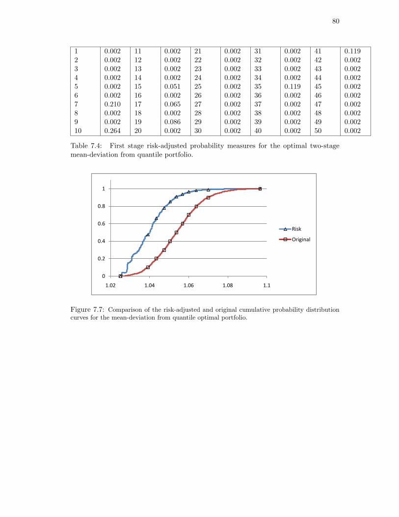
80
1 0.002 11 0.002 21 0.002 31 0.002 41 0.1192 0.002 12 0.002 22 0.002 32 0.002 42 0.0023 0.002 13 0.002 23 0.002 33 0.002 43 0.0024 0.002 14 0.002 24 0.002 34 0.002 44 0.0025 0.002 15 0.051 25 0.002 35 0.119 45 0.0026 0.002 16 0.002 26 0.002 36 0.002 46 0.0027 0.210 17 0.065 27 0.002 37 0.002 47 0.0028 0.002 18 0.002 28 0.002 38 0.002 48 0.0029 0.002 19 0.086 29 0.002 39 0.002 49 0.00210 0.264 20 0.002 30 0.002 40 0.002 50 0.002
Table 7.4: First stage risk-adjusted probability measures for the optimal two-stagemean-deviation from quantile portfolio.
0
0.2
0.4
0.6
0.8
1
1.02 1.04 1.06 1.08 1.1
Risk
Original
Figure 7.7: Comparison of the risk-adjusted and original cumulative probability distributioncurves for the mean-deviation from quantile optimal portfolio.

81
0
0.2
0.4
0.6
0.8
1
0.974 0.979 0.984 0.989 0.994 0.999
Risk
Original
Figure 7.8: Comparison of the risk-adjusted and original cumulative probability distributioncurves for the market portfolio, using the weighted mean-deviation from quantile risk function.
The risk-adjusted CDF and original CDF for the market portfolio are plotted to-
gether in Figure (7.8), were the curves are closer together than for the optimal portfolio.
The results suggest that for the two-stage mean-deviation from quantile portfolio
problem, the optimal portfolio does not perform as well as the market portfolio, from
the perspective of a risk averse investor. However, the optimal portfolio has a higher
range of end portfolio values than the market portfolio.
7.4 Comparison of Different Solution Methods
7.4.1 Setup
In this section, we compare the performance of the three solution methods for the
two-stage risk averse portfolio problem, described in (6.20), (6.31), and (6.37, 6.43).
As in the previous section, a portfolio of 100 assets was drawn from the S & P500
index. Weekly returns were constructed from daily returns, taken over 5 business
days. Scenario trees ξ1 × ξ2, of different sizes were randomly sampled. Recall that ξ1
represents the number of first stage nodes, and ξ2 represents the number of second

82
stage nodes connected to any first stage node. The following scenario trees were used:
10 × 10, 20 × 20, 50 × 40.
On each of these scenario trees, the two-stage mean-risk portfolio problem with
risk measures semideviation (5.11) and weighted deviation from quantile (5.33) was
constructed. The portfolio problem was solved using Benders’ Decomposition method
and the multi-cut Benders’ Decomposition method. Separately, the portfolio problem
was written as one large linear programming problem and solved using the simplex
method.
The performance of the three solution methods were compared along the following
dimensions: total solve time, total run time, total computer memory used, and number
of simplex iterations used.
7.4.2 Results on Solve Time
The solve times, for different sized scenario trees are displayed in Tables 7.5 and 7.6, for
the mean-semideviation and mean-weighted deviation from quantile portfolio problems,
respectively.
Scenario Linear Benders Multi10 × 10 6.453 12.507 5.99620 × 20 5.578 35.683 22.46950 × 40 7.531 326.523 65.121
Table 7.5: Comparison of total solve time for two stage mean-semideviation portfolioproblem, using different solution methods.
Scenario Linear Benders Multi10 × 10 6.345 10.769 8.19320 × 20 8.75 28.938 22.35950 × 40 6.906 235.594 166.405
Table 7.6: Comparison of total solve time for two stage mean-deviation from quantileportfolio problem, using different solution methods.
Looking at the tables, it is clear that the linear programming method outperformed
the cutting plane methods, in all three scenario trees for the quantile risk measure

83
and in all but one scenario tree for the semideviation risk measure. As the size of
the scenario tree increased, this gap in run times between the linear method and the
cutting plane methods increased substantially. Between the two cutting plane methods,
the multi-cut Benders decomposition method generally took less time to solve than the
Benders decomposition method. The gap in solve times between the two cutting plane
methods was much smaller than the gap between the linear method and any of the
cutting plane methods.
7.4.3 Results on Memory Usage
We begin this section with the results on the dimension of total memory used by the
three methods, for the two stage mean-semideviation model. The results are displayed
in Table 7.7
Scenario Linear Benders Multi10 × 10 2,813,800 2,559,752 2,302,73620 × 20 7,697,632 6,335,928 6,908,62450 × 40 31,402,560 20,914,800 27,812,564
Table 7.7: Comparison of total memory used by different solution methods, for thetwo stage mean-semideviation portfolio problem.
Looking at the table, it is evident that the total memory used by the linear method
exceeded that used in the extended Benders’ and multi-cut Benders’ methods for
all three scenario trees. The total memory used by the extended multi-cut Benders’
method was less than that used by the extended Benders’ method nad linear method
for all three scenario trees.
To obtain a better perspective on these results, a table of ratios was constructed,
for each scenario tree 7.8. The ratios are meant to compare the memory used by
one method against another. For example, a ratio was constructed with the memory
used by Benders’ Decomposition in the numerator, and the memory used by the linear
method in the denominator. Ratios comparing the memory usage of the extended multi-
cut Benders decomposition method to the linear method, and the extended Benders

84
decomposition method to the extended multi-cut Benders decomposition method were
also constructed.
By placing these ratios together for different sized scenario trees, we can see
how the memory usage depends on the size of the tree. For example, in the first
case, if the ratio decreases in size as the scenario tree increases in size, then the
Benders’ Decomposition method memory usage grow slower in proportion to the linear
programs’ memory usage. For very large programs, this may mean the Linear method
will be more likely to crash where the extended Benders’ decomposition method will
solve. The table of proportions is given below:
Scenario Benders memoryLinear memory
Multi Cut Benders memoryLinear memory
Benders memoryMulti Cut Benders memory
10 × 10 0.9097 0.8184 1.111620 × 20 0.8231 0.8975 0.917150 × 40 0.666 0.8857 0.7520
Table 7.8: Comparison of ratios for memory usage, for different solution methods, fortwo stage mean semideviation portfolio problem.
Looking at Table (7.8), it is clear that the proportion of memory used by both
the extended Benders’ decomposition method and the extended multi-cut Benders’
decomposition method, in relation to the linear method are less than one, suggesting
they use less memory than the linear method in all three scenario trees. The
proportions decrease as the scenario tree increases in size for the Benders method
comparison, and stays between 0.8 and 0.9 for the multi cut Benders comparisons.
For a scenario tree of size 500 × 200, we tested both the linear and extended Benders
decomposition methods. The linear programming method crashed because of memory
overload, while, albeit very slowly, the extended Benders’ decomposition method solved.
For the mean-deviation from quantile model, the total memory used by the three
methods is presented in Table 7.9.
The linear model used more memory than the extended multi-cut Benders’
decomposition method on all three scenario trees, and used less memory than the

85
Scenario Linear Benders Multi10 × 10 2,906,240 2,664,048 2,296,88020 × 20 7,869,800 8,669,176 6,085,06450 × 40 32,220,472 39,482,832 31,543,752
Table 7.9: Comparison of total memory used by different solution methods, for thetwo stage mean-deviation from quantile portfolio problem.
extended Benders’ decomposition method on all but one scenario tree.
As in the semideviation case, a table of proportions was constructed. The table of
these proportions is given below :
Scenario Benders memoryLinear memory
Multi Cut Benders memoryLinear memory
Benders memoryMulti Cut Benders memory
10 × 10 0.917 0.7903 1.159920 × 20 1.10 0.7732 1.424750 × 40 1.225 0.9790 1.2517
Table 7.10: Comparison of ratios for memory usage, for different solution methods,for the two stage mean deviation from quantile portfolio problem.
In the first column of Table (7.10), the ratio of memory used by extended Benders
method in relation to the linear method increases in the size of the scenario tree,albeit
somewhat slowly. The ratios in the second column, representing comparison of memory
usage by extended multi-cut Benders’ decomposition method to the linear method,
increase somewhat slowly as the scenario tree size increases. The ratio of memory used
by extended Benders’ method in relation to the extended multi-cut Benders’ method,
in the third column, stays in the range of 1.15 to 1.43.
We note that in both cases, the computer programs to solve the two stage mean risk
portfolio problems did not use the most efficient storage techniques for memory. The
optimal portfolio, first stage risk-adjusted probability measure and Lagrange multipliers
were recorded and stored for each iteration. With improved memory storage techniques,
these ratios may change.

86
7.4.4 Results on Number of Iterations
The number of outer iterations for the extended Benders and the multi-cut Benders de-
composition methods are presented in Tables 7.11 and 7.12, for the mean-semideviation
and mean-weighted deviation from quantile models, respectively.
Scenario Benders Multi10 × 10 18 720 × 20 22 1050 × 40 19 14
Table 7.11: The number of outer iterations generated in the master problem for thetwo cutting plane methods, for the two-stage mean-semideviation portfolio problem.
Scenario Benders Multi10 × 10 20 1020 × 20 37 1450 × 40 81 35
Table 7.12: The number of outer iterations generated in the master problem for thetwo cutting plane methods, for the two-stage mean-deviation from quantile portfolioproblem.
The number of outer iterations in the mean-semideviation model did not increase
substantially over the different scenario trees. The extended Benders’ method used a
larger number of outer iterations than the multi-cut Benders’ decomposition methods at
each scenario tree. For the mean-weighted deviation from quantile model, the pattern
was repeated. However, the number of outer iterations increased susbstantially, as the
size of the scenario tree increased.
7.5 Comparison of Aggregate and Conditional Risk Mapping Ap-
proach
In this section, we construct the two-stage mean-semideviation and mean-deviation
from quantile portfolio problems, with 50 outcomes in the first stage, and 40 second
stage outcomes for each first stage outcome. For the trading costs κ = 0.005 and κ = 1,
we compare the end portfolio return outcomes. The second problem is equivalent to a
one stage model with no trading. The question we are addressing is whether or not it
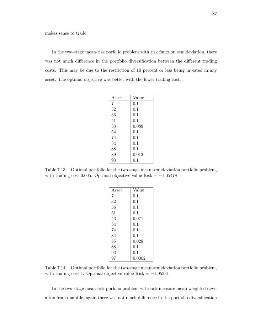
87
makes sense to trade.
In the two-stage mean-risk porfolio problem with risk function semideviation, there
was not much difference in the portfolio diversification between the different trading
costs. This may be due to the restriction of 10 percent or less being invested in any
asset. The optimal objective was better with the lower trading cost.
Asset Value7 0.132 0.136 0.151 0.153 0.08854 0.174 0.184 0.188 0.189 0.01293 0.1
Table 7.13: Optimal portfolio for the two-stage mean-semideviation portfolio problem,with trading cost 0.005. Optimal objective value Risk = −1.05478
Asset Value7 0.132 0.136 0.151 0.153 0.07154 0.174 0.184 0.185 0.02888 0.193 0.197 0.0002
Table 7.14: Optimal portfolio for the two-stage mean-semideviation portfolio problem,with trading cost 1. Optimal objective value Risk = −1.05331
In the two-stage mean-risk porfolio problem with risk measure mean weighted devi-
ation from quantile, again there was not much difference in the portfolio diversification

88
between the different trading costs. This may be due to the restriction of 10 percent
or less being invested in any asset. The optimal objective was better with the lower
trading cost.
Asset Value7 0.054 78 0.03112 0.1 84 0.0113 0.034 85 0.04618 0.038 88 0.132 0.080 89 0.02936 0.1 93 0.0651 0.07 97 0.02659 0.085 100 0.0074 0.048
Table 7.15: Optimal portfolio for the two-stage mean-deviation from quantile portfolioproblem, with trading cost 0.005. Optimal objective value, Risk = −1.03599
Asset Value7 0.052 12 0.05013 0.027 18 0.02832 0.086 36 0.151 0.076 53 0.00354 0.007 59 0.05974 0.1 84 0.093985 0.068 88 0.189 0.051 93 0.08897 0.011
Table 7.16: Optimal portfolio for the two-stage mean-deviation from quantile portfolioproblem, with trading cost 1. Optimal objective value Risk = −1.03079

89
7.6 Progress of Benders’ Decomposition
In this section, we analyze the performance of the extended Benders’ Decomposition
method on the two stage mean-risk portfolio problem, with risk function semideviation.
For a very large scenario tree (100 × 100), a graph of the gap between the optimal
solution at the kth outer iteration, and the value of the kth optimality cut function was
constructed. Recall that in the Benders’ Decomposition method, the algorithm stops
when this gap is smaller than some ε, were ε > 0. The objective was to determine how
man iterations it would take to reach an optimal solution, and how fast the method
converges.
0
0.001
0.002
0.003
0.004
0.005
0.006
0.007
0.008
0 5 10 15 20
Absolute Value of Optimality Gap
Op
tim
alit
y G
ap
Number of Cuts
Figure 7.9: Graph of optimality gap to outer iteration number, for Benders decompositionmethod, applied to mean-semideviation two-stage portfolio problem.
In figure 7.9, the method converges rapidly within the first 10 to 13 outer iterations.
After this, it will run for a very long time, making very small contributions to the
optimal solution. For larger scenario trees, this tail grows longer, and the method will
take a long time to solve.
90
Chapter 8
Conclusion
We formulated the one stage risk averse portfolio problem (2.3 ) as a zero sum matrix
game, with a new set of risk-adjusted probability measures part of the optimal saddle
point solution. Closed form solutions for the risk adjusted probability measures
were constructed, for the risk averse portfolio problem with mean-risk objective, for
the risk functions semideviation (5.10) and mean-weighted deviation from quantile
(5.31). These measures were used to evaluate the perfomance of the optimal portfolio,
compared to a market portfolio. The results suggest that the optimal portfolio
performs better than the market portfolio.
In the second part of the dissertation, we introduced the conditional risk mapping
approach to the problem of optimizing a portfolio over two investment periods, with
the option to rebalance. The resulting two-stage portfolio optimization problem was
called the two-stage risk-averse portfolio problem (4.12).
Using convex analysis, the two-stage risk averse portfolio problem was reformulated
as a zero sum matrix game, with first stage risk adjusted probability measures derived
from the optimal saddle point solution. The second stage problem was also formulated
as a zero-sum matrix game, and optimal risk adjusted probability measures were
calculated.
The first and second stage risk adjusted probability measures were calculated
for the mean-risk portfolio problem, for the risk functions semideviation (5.10) and
mean-weighted deviation from quantile (5.31). As in the first section, these measures

91
were used to evaluate the performance of the optimal portfolio, compared to a market
portfolio. The results suggest the optimal portfolio performs better.
The Benders’ Decomposition and Multi-cut Benders’ Decomposition methods for
solving a two-stage linear stochastic programming problem (6.2) were extended to
solving the two-stage risk-averse portfolio problem. On scenario trees of different sizes,
the performance of these methods and a linear programming method were compared
on the specs of total solve time, and memory usage, for both the mean-semideviation
and mean-weighted deviation from quantile models. On the specs of time, the linear
program performed better on all scenario trees. For total memory usage, the hypothesis
was that the extended Benders’ methods would use less memory in relation to the
linear program as the scenario tree size increased. This hypothesis was supported
for the mean-semideviation model. On very large scenario trees, it crashed were the
extended Benders’ method solved. Another hypothesis, that the extended multi-cut
Benders’ decomposition method would use less memory than the extended Benders’
decomposition method, was not supported for either the mean-semideviation or the
mean-weighted deviation from quantile models.
It was mentioned that the computer programs for the extended Benders’ decompo-
sition methods did not make use of the most efficient memory storage methods. In the
future, these programs could be run with better memory storage techniques, to yield
improvements on the performance of the extended Benders’ decomposition methods.
Also, for future research, it would be interesting to examine the question of which
risk measures to use in each stage of the two stage risk averse portfolio problem.
Recall we used the mean-semideviation risk measures for both objective functions in
one model, and mean deviation from quantile risk measures for both objectives in
another model. This was done for illustrative purposes, to examine how risk adjusted
probability measures could evaluate portfolio performance, and to test the extensions
on Benders’ decomposition methods. The question of what the composition of these

92
two measures means intuitively, or wether other compositions would be more useful
would be interesting to investigate further.

93
References
[1] Artzner, P., F.Delbaen, J.M.Eber and D.Heath, Thinking Coherently, Risk, 10,68-71 1997.
[2] Artzner, P., F.Delbaen, J.M.Eber and D.Heath, Coherent measures of risk, Math-ematical Finance, 9, 203-228, 1999.
[3] Artzner, P., F.Delbaen, J.M.Eber, D.Heath, and H. Ku, Multiperiod Risk andCoherent Multiperiod Risk Measurement, 2002.
[4] Acerbi C., Tasche D., Expected Shortfall: A natural coherent alternative to Valueat Risk, Economic Notes, volume 31, issue 2, 379-388, 2003.
[5] Basel Committee on Banking Supervision, The new Basel Capital Accord, BaselCommittee on Banking Supervision, Consulative Document, BIS January 2001.
[6] Brachinger, H. W., and Weber, M., Risk as a primitive: a survey of measures ofpercieved risk, Operations Research- Spektrum, 19(1997), 235-250.
[7] Domar E.V., and Musgrave R.A., Proportional Income Taxation and Risk Taking,Quart. J. Econ., 58, 389-422, May 1944.
[8] Duffie D., and J. Pan, An Overview of the Value at Risk, Journal of Derivatives,4, 7 - 49, 1997.
[9] Fishburn, PC, Mean-Risk Analysis with Risk Associated with Below-Target Re-turns, The American Economic Review, 67, 116-126, 1977.
[10] Follmer, H., and A. Schied, Convex measures of risk and trading constraints,Finance and Stochastics, 6, 429-447, 2002.
[11] Follmer, H., and A. Schied, Stochastic Finance. An Introduction in Discrete Time,de Gruyter, Berlin, 2004.
[12] Fritelli, M, and E. Rosazza Gianin, Putting order in risk measures, Journal ofBanking and Finance, 26, 1473-1486, 2002.
[13] Hanoch, G., and H., Levy, The Efficiency Analysis of Chocies Involving Risk ,Review of Economic Studies, 36, 335-346, 1969.
[14] Hardy G.H., J.E. Littlewood, and G. Polya, Inequalities, Cambridge U.K.: Cam-bridge University Press, 1934.
[15] Klein Haneveld, W.K., Duality in Stochastic Linear and Dynamic Programming,Lecture Notes in Economics and Math. Systems 274, Springer, Heidelberg, 1986.

94
[16] Kusuoka, S., On Law Invariant Coherent Risk Measures, Adv. Math. Econ., 3,83-95, 2001.
[17] Mao J.C.T., Survey of Capital Budgeting: Theory and Practice, J. Finance, 25,349-360, 1970.
[18] Markowitz, H.M. (1952): Portfolio Selection, Journal of Finance, 7, 77-91
[19] Markowitz, H.M. Portfolio Selection: Efficient Diversification of Investment, YaleUniversity Press, New Haven, USA, 1959.
[20] Mansini, R., Ogryczak, W., and M. G. Speranza, On LP solvable models for port-folio selection, Informatica, 14 (1), 37-62, 2003.
[21] Miller N. , Ruszczynski, A., Risk-Adjusted Probabilities in Portfolio Optimizationwith Coherent Risk Measures, European Journal of Operational Research, vol 191,issue 1, 193-206, 2008.
[22] Ogryczak, W., Ruszczynski, A., From Stochastic Dominance to mean-risk mod-els: Semideviations as risk measures, European Journal of Operational Research,116(1999) 33-50
[23] Ogryczak, W., Ruszczynski,A., On Consistency of Stochastic Dominance andMean-Semideviation Models, Mathematical Programming, 89, 217-232, 2001.
[24] Ogryczak, W., Ruszczynski, A., Dual Stochastic Dominance and Related Mean-Risk Models, SIAM J. on Optimization, 13 (2002), 60-78.
[25] Porter, R.B., Semivariance and Stochastic Dominance: A comparison, The Amer-ican Economic Review 64, 200-204, 1974.
[26] Porter, R.B., Gaumnitz, J.E., Stochastic Dominance v.s. Mean-Variance PortfolioAnalysis: An Empirical Evaluation, The American Economic Review, 62, 438-446,1972.
[27] Prekopa A., Stochastic Programming, Kluwer Academic Publishers, London 1995.
[28] Prekopa A., Contributions to the Theory of Stochastic Programming, Math. Prog.4, 202-221, 1973.
[29] Riedel, F., Dynamic Coherent Risk Measures, Stochastic Processes Appl., 112,185-200, 2004.
[30] Rockafellar R. T., Conjugate Duality and Optimization, SIAM, 1987.
[31] Rockafellar R.T, Uryasev, S., and M. Zabarankin, Deviation measures in risk anal-ysis and optimization, Finance and Stochastics, 10, 51-74, 2006.
[32] Rockafellar R.T, Uryasev, S., Optimization of Conditional Value at Risk, TheJournal of Risk, 2, 21-41, 2000.
[33] Rothschild, M., Stiglitz, J.E., Increasing Risk: 1 A Definition, Journal of EconomicTheory 2, 225-243, 1970.

95
[34] Ruszczynski, A, Nonlinear Optimization, Princeton University Press, Princeton2006.
[35] Ruszczynski, A. and A. Shapiro, Optimization of convex risk functions, Mathe-matics of Operations Research, 31, 433-452, 2006.
[36] Ruszczynski A. and Shapiro A., Optimization of risk measures, In Probabilistic andRandomized Methods for Design under Uncertainty, G. Calafiore and F. Dabbene,(Eds.), Springer, London, 2005
[37] Ruszczynski, A and Shapiro A., Conditional Risk Mappings, Mathematics of Op-erations Research, Vol 31, No. 3, August 2006, pp 544-561
[38] Ruszczynski, A. and R. J. Vanderbei, Frontiers of Stochastically NondominatedPortfolios, Econometrica, 71(4), 1287-1297, 2003.
[39] Ruszczynski, A. and Shapiro A., Optimality and Duality in Stochastic Program-ming,
[40] Shapiro A. and Ruszczynski, A, Lectures on Stochastic Programming, November19 2007.
[41] Cheng S., Liu Y., and Wang S., Progress in Risk Measurement, Advanced Mod-elling and Optimization, Volume 6, Number 1, 2004.
[42] Stone B.K., A General Class of Three Parameter Risk Measures, Journal of Fi-nance, 28, 675-685, 1973.
[43] Tasche D., Expected Shortfall and Beyond, Journal of Banking and Finance, 26,1519-1533, 2002.
[44] Tobin J., Liquidity Preferences as a Behaviour Toward Risk, Review of EconomicStudies, 25, 65-86, 1958.
[45] Whitmore, G.A., Mc. (Eds.), Stochastic Dominance: An Approach to Decision-Making Under Risk, Heath, Lexington M.A. 1978.
[46] Yamai Y. and Yoshiba T., Comparitive analyses of expected shortfall and Value-at-Risk under Market Stress, Monetary and Economic Studies, volume 20, 3, 181-237,2002.
[47] Yitzhaki S., Stochastic Dominance, Mean Variance and Gini’s Mean-Difference,The American Economic Review, 72, 178-185, 1982.

96
Vita
Naomi Miller
2004-2008 Ph.D. in Operations Research, Rutgers University
1999-2003 B. Sc. (Hons.) Mathematics, University of Toronto
2007-2008 Teaching Assistant Rutgers University, 1st year Calculus and Pre-calculus
2006-2007 Research Assistant, Rutgers University
2008 Miller N. , Ruszczynski, A., Risk-Adjusted Probabilities in Portfolio Opti-mization with Coherent Risk Measures, European Journal of OperationalResearch, vol 191, issue 1, 193-206,

![Portfolio Optimization Using Fundamental Indicators Based ...€¦ · Ratio, Value at Risk (VaR), the Mean (Portfolio Expected Return), and the variance [3]. Tettamanzi & Loraschi](https://img.pdfslide.net/doc/110x75/5ec6b36063a53b6c3429a05f/portfolio-optimization-using-fundamental-indicators-based-ratio-value-at-risk.jpg)