Embed Size (px)
Citation preview
LEIDEN UNIVERSITY
MASTER THESIS
Robust Mean-Variance Optimization
Author:T.A. DE GRAAF
Supervisors:Dr. O.W VAN GAANS
(M.I. Leiden)
Dr. M. VAN DER SCHANS(Ortec Finance)
December 2, 2016

iii
LEIDEN UNIVERSITY
Abstract
Robust Mean-Variance Optimization
by T.A. DE GRAAF
Mean-Variance optimization is widely used to find portfolios that make an optimal trade-off between expected return and volatility. The method, however, struggles with a ro-bustness problem since the portfolio weights are very sensitive towards change of theinput parameters. There is a vast literature on methods that tries to solve this prob-lem and we discuss two of these methods: resampling and shrinkage. In addition to themethods from the literature, we develop a new method which we call maximum distanceoptimization.
The resampling method attempts to obtain more robust portfolios by changing the opti-mization procedure. The shrinkage method attempts to obtain more robust portfolios bymaking the estimation of the input parameters more robust. The maximum distance op-timization method explores a region closely beneath the efficient frontier and determineswhat kind of portfolios are nearly optimal, but have very different portfolio weights.First, we show that any convex combination of these near-optimal portfolios is also nearoptimal. Second, we show that the set of near-optimal portfolios is robust. Apart fromthe robustness, the advantage of this method is that we now obtain a whole scope of so-lutions, instead of a single portfolio, which Mean-Variance optimization provides. Sincethe region is robust, the investor or consultant can use his own qualitative arguments toselect a preferred portfolio from this region.

v
Contents
Introduction 1
1 Mean-Variance optimization 31.1 Formulation . . . . . . . . . . . . . . . . . . . . . . . . . . . . . . . . . . . . 31.2 Analysis of Mean-Variance optimization . . . . . . . . . . . . . . . . . . . . 51.3 Robustness problems . . . . . . . . . . . . . . . . . . . . . . . . . . . . . . . 9
1.3.1 The effect of errors in returns, variances, and correlations . . . . . . 91.3.1.1 Conclusion . . . . . . . . . . . . . . . . . . . . . . . . . . . 17
2 Resampling 192.1 Formulation . . . . . . . . . . . . . . . . . . . . . . . . . . . . . . . . . . . . 202.2 Example . . . . . . . . . . . . . . . . . . . . . . . . . . . . . . . . . . . . . . 22
2.2.1 The diversification effect of resampling . . . . . . . . . . . . . . . . 232.2.1.1 Conclusion . . . . . . . . . . . . . . . . . . . . . . . . . . . 27
2.2.2 The robustness effect of resampling . . . . . . . . . . . . . . . . . . 272.2.2.1 Conclusion . . . . . . . . . . . . . . . . . . . . . . . . . . . 35
2.2.3 Convexity in the resampled frontier . . . . . . . . . . . . . . . . . . 352.2.3.1 Conclusion . . . . . . . . . . . . . . . . . . . . . . . . . . . 39
3 Shrinkage 413.1 Formulation . . . . . . . . . . . . . . . . . . . . . . . . . . . . . . . . . . . . 413.2 Data . . . . . . . . . . . . . . . . . . . . . . . . . . . . . . . . . . . . . . . . . 423.3 Linear shrinkage . . . . . . . . . . . . . . . . . . . . . . . . . . . . . . . . . 43
3.3.1 Constant correlation target . . . . . . . . . . . . . . . . . . . . . . . 433.3.2 The robustness effect of shrinkage . . . . . . . . . . . . . . . . . . . 47
3.3.2.1 Conclusion . . . . . . . . . . . . . . . . . . . . . . . . . . . 52
4 Maximum distance optimization 534.1 Maximum distance towards convex hull . . . . . . . . . . . . . . . . . . . . 544.2 Support Vector Machines . . . . . . . . . . . . . . . . . . . . . . . . . . . . . 554.3 Formulation of maximum distance optimization . . . . . . . . . . . . . . . 574.4 Basin hopping . . . . . . . . . . . . . . . . . . . . . . . . . . . . . . . . . . . 60
4.4.1 Starting point . . . . . . . . . . . . . . . . . . . . . . . . . . . . . . . 604.4.2 Number of iterations . . . . . . . . . . . . . . . . . . . . . . . . . . . 614.4.3 Stepsize . . . . . . . . . . . . . . . . . . . . . . . . . . . . . . . . . . 614.4.4 Temperature . . . . . . . . . . . . . . . . . . . . . . . . . . . . . . . . 614.4.5 Local minimization algorithm . . . . . . . . . . . . . . . . . . . . . . 624.4.6 Basin hopping pseudocode . . . . . . . . . . . . . . . . . . . . . . . 62
4.5 Example . . . . . . . . . . . . . . . . . . . . . . . . . . . . . . . . . . . . . . 634.5.1 Extra stop criterion . . . . . . . . . . . . . . . . . . . . . . . . . . . . 634.5.2 Results . . . . . . . . . . . . . . . . . . . . . . . . . . . . . . . . . . . 644.5.3 Convex combination portfolio . . . . . . . . . . . . . . . . . . . . . 704.5.4 The diversification effect of MDO . . . . . . . . . . . . . . . . . . . 71

vi
4.5.4.1 Conclusion . . . . . . . . . . . . . . . . . . . . . . . . . . . 724.5.5 Norms for determining the robustness of MDO . . . . . . . . . . . 724.5.6 The robustness effect of MDO . . . . . . . . . . . . . . . . . . . . . . 74
4.5.6.1 Conclusion . . . . . . . . . . . . . . . . . . . . . . . . . . . 78
5 Applications 795.1 Shrinkage . . . . . . . . . . . . . . . . . . . . . . . . . . . . . . . . . . . . . 795.2 Resampling . . . . . . . . . . . . . . . . . . . . . . . . . . . . . . . . . . . . 79
5.2.1 Advice . . . . . . . . . . . . . . . . . . . . . . . . . . . . . . . . . . . 805.3 Maximum distance optimization . . . . . . . . . . . . . . . . . . . . . . . . 80
5.3.1 Advice . . . . . . . . . . . . . . . . . . . . . . . . . . . . . . . . . . . 81
1
Introduction
Investors can invest their money in a wide variety of asset classes. All asset classes havetheir own characteristics and investors want to make smart decisions. They aim to opti-mize their portfolio by taking into account the historical performances of the asset classesand decide what proportion of their investment-budget they want to invest in which as-set class.
In 1952, Harry Markowitz introduced a groundbreaking method regarding portfolio op-timization in his paper ‘Portfolio Selection’ [8]. Despite an initial lack of interest, theideas he present have come to build foundations on the nowadays widely used Mean-Variance optimization method. In 1990, Markowitz, together with William Sharpe andMerton Miller, even received the Nobel Memorial Prize in Economic Sciences for theircontribution in the theory of financial economics [9].
Mean-Variance optimization uses expected return (mean) as a measure for profit and ex-pected volatility (variance) as a risk measure. From historical performances, we can esti-mate the expected risk and the expected return of an asset class, as well as the correlationbetween the asset classes. Based on these performances, Mean-Variance optimization canbe used to construct portfolios that have an optimal balance between required expectedreturn and the level of risk that an investor is willing to take.
There are two disadvantages to Mean-Variance optimization. The most important oneis that this method is sensitive towards adjustments of the input. For example, a smallchange of the expected return of one asset class, can result in a totally different optimalportfolio allocations. Investors do not want to change their investment strategy drasti-cally, due to reasons as liquidity problems and transaction costs. Hence, it is undesirablethat sightly different modeling assumptions lead to completely different allocation deci-sions. In this thesis, we are searching for a way to tackle this problem, that is, a way tomake the Mean-Variance optimization method more robust. The second disadvantageis that in Mean-Variance optimization, we can obtain portfolios that are little diversi-fied. The concept of not putting all eggs into one basket is a conventional wisdom thatinvestors like to follow, hence we want to obtain more diversified portfolios.
In this thesis, we discuss three methods that try to solve the robustness problem of Mean-Variance optimization. In Chapter 2, we discuss a method called resampling [10]. InChapter 3, we discuss a method called shrinkage [6]. In Chapter 4, we develop a newmethod which we call maximum distance optimization. In Chapter 5, we discuss theapplications of these three methods and formulate our advice to Ortec Finance.

3
Chapter 1
Mean-Variance optimization
Mean-Variance optimization is a widely used method for portfolio optimization. Fordifferent risk aversion levels, we obtain portfolios with an optimal tradeoff between ex-pected volatility and expected return. It is known that Mean-Variance optimization strug-gles with a robustness problem: small changes of the estimated input parameters canresult in different optimal portfolio weights. A second problem that we can encounteris that we can obtain optimal portfolios that are little diversified. In this section, we firstgive a formal definition of Mean-Variance optimization and then we show the robustnessand diversification problems that we encounter.
1.1 Formulation
Consider N ∈ N asset classes of which we assume that their returns, r ∈ RN , are nor-mally distributed, with mean µ ∈ RN , and covariance matrix Σ ∈ RN × RN . We knowthat Σ is semi positive definite by definition. Here, we assume that it is positive definite.In reality, no asset class is an exact linear combination of other asset classes, so this is areasonable assumption. Let w ∈ RN denote the weight vector, or portfolio, then µ0 = wᵀµrepresents the expected portfolio return, σ20 = wᵀΣw represents the expected portfolio risk,and r0 = wᵀr represents the real portfolio return, which we assume to be normally dis-tributed with r0 ∼ N (µ0, σ
20). Sometimes the expected portfolio return and the expected
portfolio risk are referred to as ‘portfolio return’ and ‘portfolio risk’, or just as ‘return’and ‘risk’, respectively. Since we are not able to predict the future, the reader knowsfrom the context what is meant. Except for the designations above, we denote the weightvector, w, also in other ways: we say ‘weights’, or ‘solution’. In the latter case, from thecontext it is clear that we consider a weight vector that is a solution to Mean-Variance(MV) optimization, or another optimization program.
Unless stated otherwise, we only regard risky assets. We can choose from a wide rangeof asset classes, all with their own characteristics. Some asset classes have generally alow risk, like German government bonds. However, one usually obtains little reward fortaking little risk. Other asset classes, like U.S. equity, have a high volatility, hence, they areconsidered to be risky. But, in return for taking more risk, one usually gets more return.Often, by investing in different asset classes with comparable risk and return levels, wecan reduce the overall portfolio risk. The question is: what asset class should get howmuch weight, to optimize the return and risk level? For a range of different return andrisk levels, the MV optimization method produces corresponding optimal portfolios.
We can choose a level of return that we require and minimize the corresponding level ofrisk. Or, we can choose the level of risk we are willing to take and maximize the level
4 Chapter 1. Mean-Variance optimization
of return. A third option is that we choose a level of risk aversion and optimize thecorresponding ratio between the risk and return level. We make these different ways offormulating MV optimization explicit in the following definitions. Later in this section,we show under which circumstances these definitions are equivalent.
Let us fix N , r, µ, and Σ as at the beginning of this subsection. We look for a weightvector w which is optimal in terms of expected volatility and return.
Definition 1.1.1. The minimum risk formulation of MV optimization is given by
minw∈RN
wᵀΣw, subject to wᵀµ = µ0, wᵀ1 = 1. (1.1)
Definition 1.1.2. The maximum return formulation of MV optimization is given by
maxw∈RN
wᵀµ, subject to wᵀΣw = σ20, wᵀ1 = 1. (1.2)
Definition 1.1.3. Let λ ∈ [0,∞), the risk aversion formulation of MV optimization is givenby
minw∈RN
λwᵀΣw −wᵀµ, subject to wᵀ1 = 1. (1.3)
There is one constraint that we left out of these definitions, but which is in some casesrequired. This constraint prevents weights from attaining a negative value: w ≥ 0. Infinancial terms, a negative weight of an asset class is called selling short or going short.Short selling is a risky business and forbidden for many investors. The constraint thatprevents us from short selling can make the analysis more complex; that is why it issometimes left out. In the definitions below, the constraint is also left out, but one canadd it if required.
The feasible set corresponding to the expected portfolio return and risk is the set parame-terized by {(σ20, µ0) : there exists w ∈ RN such that σ20 = wᵀΣw, µ0 = wᵀµ, and wᵀ1 =1}. To define the optimal portfolios in an unambiguous way, we first have to look atthe solution with minimal variance. Let wGMV be such that wGMV = arg minw∈RN wᵀΣwand wᵀ
GMV1 = 1, then wGMV is called the global minimum variance (GMV) portfolio. DefineµGMV = wᵀ
GMVµ as the global minimum (expected) return and σ2GMV = wᵀGMVΣwGMV as the global
minimum (expected) risk.
Definition 1.1.4. A weight vector w is called efficient or optimal, if w is a solution to (1.1)for some µ0 ≥ µGMV, or if it is a solution to (1.2) for some σ20 ≥ σ2GMV, or if it is a solution to(1.3) for some λ ∈ [0,∞).
Define W = {w : w is an efficient weight vector} as the set of efficient weights. In Lemma1.2.7, we show that, regarding only efficient weights, the three formulations, (1.1), (1.2),and (1.3), are equivalent. Hence, the definition of an optimal weight vector is unambigu-ous.
Definition 1.1.5. The efficient frontier is given by
{(σ20, µ0) : σ20 = wᵀΣw, µ0 = wᵀµ, w ∈W}.
Figure 1.1 gives a graphical interpretation of the definitions above.
1.2. Analysis of Mean-Variance optimization 5
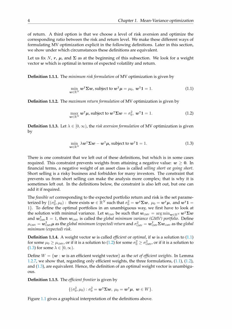
FIGURE 1.1: The efficient frontier, together with the global minimum vari-ance portfolio and the feasible set.
σ20
µ0Efficient frontier
Feasible setµGMV wGMV
σ2GMV
The amount of risk one is willing to take is represented by the risk aversion parameter.If λ = 0, we do not care about risk at all and we are only interested in maximizingthe expected return, wᵀµ. If λ is big, we are more focused on low risk than on highreturn. By taking λ in a range from zero to infinity, we get optimal portfolios, rangingfrom µGMV and σGMV, to maxn≤N µn and corresponding risk. It seems reasonable to want aportfolio somewhere in between these extremes. By looking at the efficient frontier anddetermining what level of risk and return fits our needs, we can figure out what riskaversion parameter suits us. However, if we include other asset classes for example, itmight be possible that the same risk aversion level puts us in another risk and/or returnposition.
1.2 Analysis of Mean-Variance optimization
In this section, we use the minimum risk formulation (1.1). We list a set of lemmas andcorollaries that help us understand MV optimization better and that are useful in lateranalyses. Note that we can invert the covariance matrix Σ, because we assume that it ispositive definite and not just semi positive definite.
Lemma 1.2.1. Assume we are allowed to go short. Let µ0 ∈ R>µGMV . The efficient portfolios wproduced by MV optimization satisfy w = g + hµ0, with
g =1
ac− b2Σ−1[c1− bµ]
h =1
ac− b2Σ−1[aµ− b1]
a = 1ᵀΣ−11
b = 1ᵀΣ−1µ
c = µᵀΣ−1µ.
Proof. We use Lagrange multipliers. Define F (w, φ1, φ2) = wᵀΣw − φ1(wᵀµ − µ0) −
φ2(wᵀ1− 1). Differentiating and setting equal to 0, gives
2Σw − φ1µ− φ21 = 0
wᵀµ− µ0 = 0
wᵀ1− 1 = 0.
6 Chapter 1. Mean-Variance optimization
The first equation can be written as
w =1
2Σ−1[µ, 1]
[φ1φ2
]. (1.4)
Using a, b, and c, defined as above, we obtain
µ0 = wᵀµ =1
2φ1c+
1
2φ2b
1 = wᵀ1 =1
2φ1b+
1
2φ2a.
Rewrite this as1
2
[φ1φ2
]=
[c bb a
]−1 [µ01
].
Putting this again in equation (1.4) gives
w = Σ−1[µ,1]
[c bb a
]−1 [µ01
]= g + hµ0.
Note that the elements in g sum up to 1 and the elements of h sum up to zero:
1ᵀg =1
ac− b2(a1ᵀΣ−11− b1ᵀΣ−1µ) = 1
1ᵀh =1
ac− b2(a1ᵀΣ−1µ− b1ᵀΣ−11) = 0.
Also, note that the positive definiteness of Σ implies that a, c > 0.
Corollary 1.2.2. Assume we are allowed to go short. If we only consider efficient portfolios, thenthe portfolio return, as a function of the portfolio risk, is given by
µ0(σ20) =
−gᵀΣh+√
(gᵀΣh)2 − (hᵀΣh)(gᵀΣg − σ20)
hᵀΣh.
Proof. We have the following functions. The risk as function of the weight vector: σ20(w) :RN → R,w 7→ wᵀΣw, the return as a function of the weight vector: µ0(w) : RN →R,w 7→ wᵀµ, and from Lemma 1.2.1, the weight vector as a function of the requiredreturn: w(µ0) : R → RN , µ0 7→ g + hµ0. Compute σ20(w(µ0)) : R → RN → R, µ0 7→g + hµ0 7→ (g + hµ0)
ᵀΣ(g + hµ0). We obtain
σ20(µ0) = wᵀ(µ0)Σw(µ0)
= µ20hᵀΣh+ µ0(g
ᵀΣh+ hᵀΣg) + gᵀΣg.
Note that this is a convex parabola, since Σ is positive definite. We obtain µ0(w(σ20)) :R→ RN → R, σ20 7→ g + hµ0 7→ µ0, by inverting the equation above:
µ0(σ20) =
−gᵀΣh±√
(gᵀΣh)2 − (hᵀΣh)(gᵀΣg − σ20)
hᵀΣh.
We leave out the ‘−’ variant as we are only interested in the highest possible return.
1.2. Analysis of Mean-Variance optimization 7
Lemma 1.2.3. Σ−1 is positive definite.
Proof. Let z ∈ RN , and take x = Σ−1z. Then
zᵀΣ−1z = (ΣΣ−1z)ᵀΣ−1z = (Σ−1z)ᵀΣᵀΣ−1z = xᵀΣᵀx = xᵀΣx > 0.
Lemma 1.2.4. For a, b, and c, defined as in Lemma 1.2.1, we have: ac− b2 ≥ 0.
Proof. The positive definite matrix Σ−1 generates an inner product: 〈x,y〉Σ−1 = xᵀΣ−1y,for x,y ∈ RN . Use Cauchy-Schwarz to show that
b2 = (1ᵀΣ−1µ)2 = (〈1,µ〉Σ−1)2 ≤ (||1||Σ−1 ||µ||Σ−1)2 = (1ᵀΣ−11)(µᵀΣ−1µ) = ac.
Lemma 1.2.5. Assume we are allowed to go short. If we only consider efficient portfolios, thenthe functions, σ20(µ0) and µ0(σ20), in terms of a, b, and c, are given by
σ20(µ0) =1
ac− b2(aµ20 − 2bµ0 + c) (1.5)
µ0(σ20) =
b
a+
1
a
√(−b2 + ac)(aσ20 − 1).
Proof. Multiply equation (1.4) by [µ, 1]ᵀ:
1
2
[µᵀ
1ᵀ
]Σ−1[µ, 1]
[φ1φ2
]=
[µᵀ
1ᵀ
]w
1
2
[φ1φ2
]=
[c bb a
]−1 [µ01
]using [
µᵀ
1ᵀ
]Σ−1[µ, 1] =
[c bb a
].
Put the attained equation for [φ1, φ2]ᵀ back in equation (1.4):
w = Σ−1[µ, 1]
[c bb a
]−1 [µ01
]. (1.6)
Use σ20 = wᵀΣw to see that
σ20 =
[Σ−1[µ, 1]
[c bb a
]−1 [µ01
] ]ᵀΣ
[Σ−1[µ, 1]
[c bb a
]−1 [µ01
] ]=
1
ac− b2(aµ20 − 2bµ0 + c).
Write µ0 as a function of σ20 :
µ0(σ20) =
b
a± 1
a
√(−b2 + ac)(aσ20 − 1).
Again we leave out the ‘−’ variant, as we want maximum return.
8 Chapter 1. Mean-Variance optimization
Corollary 1.2.6. Assume we are allowed to go short. We obtain σ2GMV = 1/a, µGMV = b/a, withweight vector wGMV = (1/a)Σ−11.
Proof. An optimum is attained when dσ20(µ0)/dµ0 = 0, that is, when (ac − b2)/(2aµ0 −2b) = 0. Use Lemma 1.2.4 to see that we are dealing with a minimum:
d2σ20(µ0)
dµ20=
2a
ac− b2> 0.
Hence, µGMV = b/a and σ2GMV = 1/a. From equation (1.6) we obtain:
wGMV =1
ac− b2Σ−1[µ,1]
[a −b−b c
] [ba1
]=
1
aΣ−11.
Lemma 1.2.7. Assume we are allowed to go short. Formulations, (1.1), (1.2), and (1.3), areequivalent if we consider only efficient portfolios.
Proof. Let w1 and w2 be efficient portfolios, with w1 6= w2. First, we show that we have
wᵀ1Σw1 < w
ᵀ2Σw2 if and only if wᵀ
1µ < wᵀ2µ. (1.7)
Suppose wᵀ1µ < wᵀ
2µ, then function (1.5) implies that σ20(wᵀ1µ) < σ20(wᵀ
2µ). Similarly,when we assume wᵀ
1Σw1 < wᵀ2Σw2, we get wᵀ
1µ < wᵀ2µ.
We now prove the equivalence of the three formulations. Suppose w1 is the solution to(1.1), given some µ0 ≥ µGMV. For formulation (1.2), we fix σ20 = wᵀ
1Σw1. We know thatwᵀ
11 = 1, hence wᵀ1µ ≤ maxww
ᵀµ. Also, according to (1.7), there can not be an efficientportfolio w2, such that wᵀ
2µ > wᵀ1µ = µ0 and wᵀ
2Σw2 = σ20 . Hence, w1 is the solution to(1.2), for σ20 = wᵀ
1Σw1.
One can use the same line of reasoning to show that a solution to (1.2), is also a solutionto (1.1). What is left to show is that the risk aversion formulation is also equivalent toformulations, (1.1) and (1.2).
Supposew1 is the solution to (1.1) and (1.2), for some µ0 = wᵀ1µ and σ20 = wᵀ
1Σw1. Usingfunction (1.5), the risk aversion formulation becomes equivalent to minimizing:
λ1
ac− b2(aµ20 − 2bµ0 + c)− µ0.
Differentiate to µ0, set it equal to 0, and solve it for λ. We get
λ =ac− b2
2aµ0 − 2b.
Suppose that w2 is such that λwᵀ2Σw2 − wᵀ
2µ < λwᵀ1Σw1 − wᵀ
1µ. Make a distinctionbetween the return of w1 and w2, by defining them as µ0,1 and µ0,2, respectively. We get
λ1
ac− b2(aµ20,2 − 2bµ0,2 + c)− µ0,2 < λ
1
ac− b2(aµ20,1 − 2bµ0,1 + c)− µ0,1
(µ0,2 − µ0,1)2 < 0.
This gives a contradiction. Hence,w1 is the solution to (1.3) for λ = (ac− b2)/(2aµ0−2b).
1.3. Robustness problems 9
Lastly, let λ ∈ [0,∞) and suppose w1 is the solution to (1.3), i.e.,
λwᵀ1Σw1 −wᵀµ ≤ λwᵀΣw −wᵀµ, for all w such that wᵀ1 = 1, w 6= w1.
Let µ0 = wᵀ1µ. Suppose thatw2 is such thatwᵀ
2µ = µ0, andwᵀ2Σw2 ≤ wᵀ
1Σw1. Then, weget λwᵀ
2Σw2 − µ0 ≤ λwᵀ1Σw1 − µ0, which gives us a contradiction to w1 being optimal.
So w1 is the solution to (1.1), and therefore also to (1.2).
1.3 Robustness problems
In this section, we show what problems we encounter in MV optimization, with regard torobustness. The main reason for wanting the MV method to be more robust is that we donot want to change a portfolio drastically due to small changes in estimated parameters.Suppose we have a current portfolio that is obtained from MV optimization and we havea large share in some asset class A. Suppose there is another asset class, B, that behavessimilarly but slightly worse, that is, suppose the correlation with A is high, the risk levelis the same, and the expected return is almost as good as that of A. If in some time periodB is outperforming A, it is possible that repeating the MV optimization procedure, basedon the new performances, results in a totally different portfolio: a small share in A anda large share in B. What should we do in this case? If we change our portfolio, we areforced to accept the transaction costs, hoping that this was just a one time occurrence. Orwe can keep our original portfolio, not knowing whether it is still representative or not.Clearly, we want to avoid such a situation. Making the MV procedure more robust willhelp, because then the sudden change in performance of asset classes has less influenceon the outcome. Also, having initially a more diversified portfolio will help, because thenwe would probably already have split the weights between asset class A and B, to someratio.
In the analyses below, we only discuss the robustness problem and omit any diversifica-tion issues. This is because diversification might help in becoming more robust, as weargue above, but tackling the robustness problem is our number one priority.
1.3.1 The effect of errors in returns, variances, and correlations
We make the robustness problem explicit through an example based on a paper of Chopraand Ziemba [3]. This paper claims that variations of the expected return vector have amuch bigger effect than variations in variances or the correlation matrix. Table 1.1 givesan overview of the expected returns and covariance matrix of 10 securities, rounded up totwo digits. These securities are: Aluminium Co. of America, American Express Co., Boe-ing Co., Chevron Co., Coca Cola Co., E.I. Du Pont De Nemours & Co., Minnesota Mon-ing and Manufacturing Co., Procter & Gamble Co., Sears, Roebuck & Co., and UnitedTechnologies Co. These securities are randomly selected from 29 Dow Jones IndustrialAverage securities, of which monthly observations from 1980 till 1989 are available.
Note that we look at one asset class: equity. One can perform the MV optimizationmethod on all different kind of selections. Usually we search for a combination of dif-ferent, safe and risky, asset classes. But if we want to choose between some selectedassets of the same asset class, we can also perform MV optimization on these individualassets.
10 Chapter 1. Mean-Variance optimization
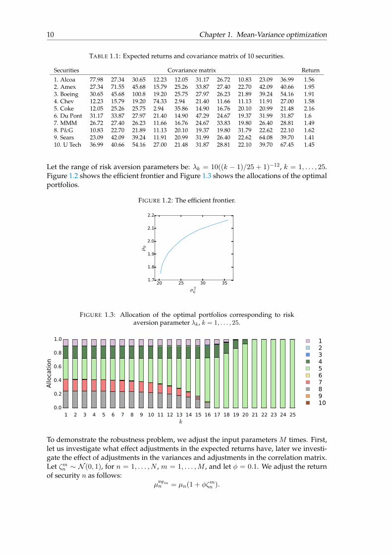
TABLE 1.1: Expected returns and covariance matrix of 10 securities.
Securities Covariance matrix Return
1. Alcoa 77.98 27.34 30.65 12.23 12.05 31.17 26.72 10.83 23.09 36.99 1.562. Amex 27.34 71.55 45.68 15.79 25.26 33.87 27.40 22.70 42.09 40.66 1.953. Boeing 30.65 45.68 100.8 19.20 25.75 27.97 26.23 21.89 39.24 54.16 1.914. Chev 12.23 15.79 19.20 74.33 2.94 21.40 11.66 11.13 11.91 27.00 1.585. Coke 12.05 25.26 25.75 2.94 35.86 14.90 16.76 20.10 20.99 21.48 2.166. Du Pont 31.17 33.87 27.97 21.40 14.90 47.29 24.67 19.37 31.99 31.87 1.67. MMM 26.72 27.40 26.23 11.66 16.76 24.67 33.83 19.80 26.40 28.81 1.498. P&G 10.83 22.70 21.89 11.13 20.10 19.37 19.80 31.79 22.62 22.10 1.629. Sears 23.09 42.09 39.24 11.91 20.99 31.99 26.40 22.62 64.08 39.70 1.4110. U Tech 36.99 40.66 54.16 27.00 21.48 31.87 28.81 22.10 39.70 67.45 1.45
Let the range of risk aversion parameters be: λk = 10((k − 1)/25 + 1)−12, k = 1, . . . , 25.Figure 1.2 shows the efficient frontier and Figure 1.3 shows the allocations of the optimalportfolios.
FIGURE 1.2: The efficient frontier.
20 25 30 35
σ 20
1.7
1.8
1.9
2.0
2.1
2.2
µ0
FIGURE 1.3: Allocation of the optimal portfolios corresponding to riskaversion parameter λk, k = 1, . . . , 25.
1 2 3 4 5 6 7 8 9 10 11 12 13 14 15 16 17 18 19 20 21 22 23 24 25k
0.0
0.2
0.4
0.6
0.8
1.0
Allo
cati
on
12345678910
To demonstrate the robustness problem, we adjust the input parameters M times. First,let us investigate what effect adjustments in the expected returns have, later we investi-gate the effect of adjustments in the variances and adjustments in the correlation matrix.Let ζmn ∼ N (0, 1), for n = 1, . . . , N , m = 1, . . . ,M , and let φ = 0.1. We adjust the returnof security n as follows:
µinpmn = µn(1 + φζmn ).
1.3. Robustness problems 11
Denote the new return vector by µinpmᵀ = [µinpm1 , . . . , µ
inpmN ]. Note that a typical deviation
of µinpmn from µn is a deviation of order φ. This is because the standard deviation is 1 and
we multiply by a factor of φ.
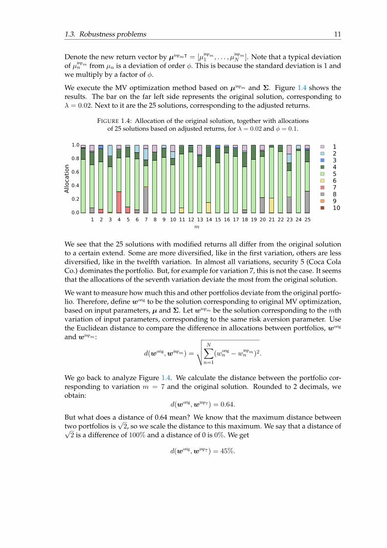
We execute the MV optimization method based on µinpm and Σ. Figure 1.4 shows theresults. The bar on the far left side represents the original solution, corresponding toλ = 0.02. Next to it are the 25 solutions, corresponding to the adjusted returns.
FIGURE 1.4: Allocation of the original solution, together with allocationsof 25 solutions based on adjusted returns, for λ = 0.02 and φ = 0.1.
1 2 3 4 5 6 7 8 9 10 11 12 13 14 15 16 17 18 19 20 21 22 23 24 25m
0.0
0.2
0.4
0.6
0.8
1.0
Allo
cati
on
12345678910
We see that the 25 solutions with modified returns all differ from the original solutionto a certain extend. Some are more diversified, like in the first variation, others are lessdiversified, like in the twelfth variation. In almost all variations, security 5 (Coca ColaCo.) dominates the portfolio. But, for example for variation 7, this is not the case. It seemsthat the allocations of the seventh variation deviate the most from the original solution.
We want to measure how much this and other portfolios deviate from the original portfo-lio. Therefore, define worig to be the solution corresponding to original MV optimization,based on input parameters, µ and Σ. Let winpm be the solution corresponding to the mthvariation of input parameters, corresponding to the same risk aversion parameter. Usethe Euclidean distance to compare the difference in allocations between portfolios, worig
and winpm :
d(worig,winpm) =
√√√√ N∑n=1
(worign − winpm
n )2.
We go back to analyze Figure 1.4. We calculate the distance between the portfolio cor-responding to variation m = 7 and the original solution. Rounded to 2 decimals, weobtain:
d(worig,winp7) = 0.64.
But what does a distance of 0.64 mean? We know that the maximum distance betweentwo portfolios is
√2, so we scale the distance to this maximum. We say that a distance of√
2 is a difference of 100% and a distance of 0 is 0%. We get
d(worig,winp7) = 45%.
12 Chapter 1. Mean-Variance optimization
This is a big difference. However, for other variations is the difference smaller. Hence,we want to calculate the average distance over all variations. Define
d(worig,winp) =1
M
M∑m=1
d(worig,winpm).
We also want to know the standard deviation of these distances:
Sd(d(worig,winp)) =
√√√√ 1
M
M∑m=1
(d(worig,winpm)− d(worig,winp))2.
For these 25 variations we obtain
d(worig,winp) = 0.20
Sd(d(worig,winp)) = 0.15.
Scaled to√
2, this becomes
d(worig,winp) = 14%
Sd(d(worig,winp)) = 11%.
Secondly, let us see what influence adjusting the variances has. We have variance σ2n,n ofcovariance matrix Σ = (σ2n,n). This time, we leave the expected returns and the corre-lation matrix untouched and solve the MV optimization problem for adjusted variances.Let
(σinpmn,n )2 = σ2n,n(1 + φζmn )
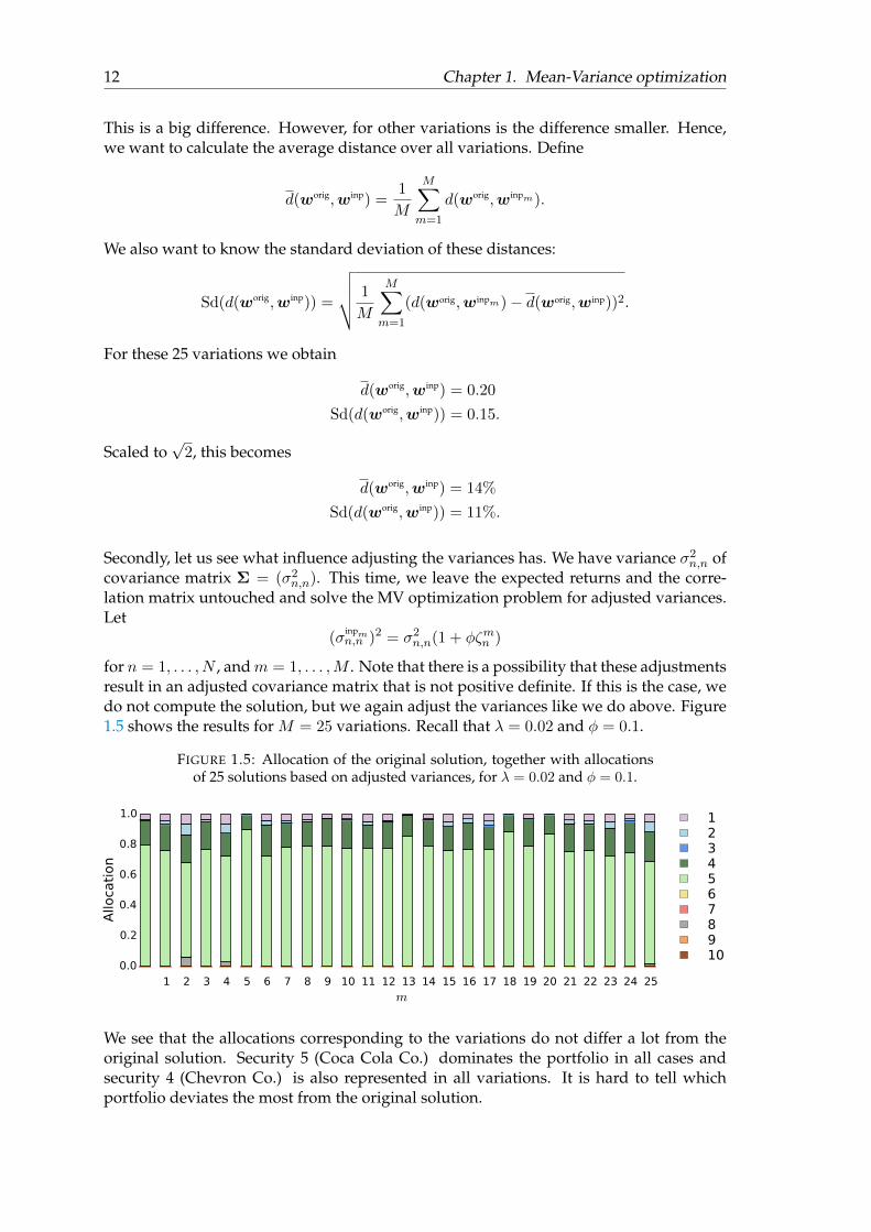
for n = 1, . . . , N , andm = 1, . . . ,M . Note that there is a possibility that these adjustmentsresult in an adjusted covariance matrix that is not positive definite. If this is the case, wedo not compute the solution, but we again adjust the variances like we do above. Figure1.5 shows the results for M = 25 variations. Recall that λ = 0.02 and φ = 0.1.
FIGURE 1.5: Allocation of the original solution, together with allocationsof 25 solutions based on adjusted variances, for λ = 0.02 and φ = 0.1.
1 2 3 4 5 6 7 8 9 10 11 12 13 14 15 16 17 18 19 20 21 22 23 24 25m
0.0
0.2
0.4
0.6
0.8
1.0
Allo
cati
on
12345678910
We see that the allocations corresponding to the variations do not differ a lot from theoriginal solution. Security 5 (Coca Cola Co.) dominates the portfolio in all cases andsecurity 4 (Chevron Co.) is also represented in all variations. It is hard to tell whichportfolio deviates the most from the original solution.
1.3. Robustness problems 13
It seems that adjusting the variances has less influence than adjusting the returns. How-ever, we can not conclude this right away, since the amount of deviation is influenced bythe value of the random parameter, ζmn . If, by coincidence, we have ζmn close to 0 for allm, then Σinpm deviates little from Σ. Therefore, it is likely that we obtain solutions thatdo not deviate much from the original solution. To reduce the influence of ζmn , we shouldcalculate d(worig,winp) and Sd(d(worig,winp)), based on a large number of variations. Wedo a more extensive analysis below, but first, we analyze these 25 variations. Scaled to√
2, we obtain
d(worig,winp) = 4.1%
Sd(d(worig,winp)) = 3.4%.
We see that these 25 portfolios, based on variations of the variances, are indeed closer tothe original portfolio than the 25 portfolios based on variations of the return vector.
Lastly, let us investigate the influence of changing the correlation matrix. Denote thecorrelation matrix by P = (ρn,n′). Let ζmn,n′ ∼ N (0, 1), for n, n′ = 1, . . . , N , and m =1, . . . ,M . For n 6= n′, let
ρinpmn,n′ = ρ
inpmn′,n = ρn,n′(1 + φζmn,n′).
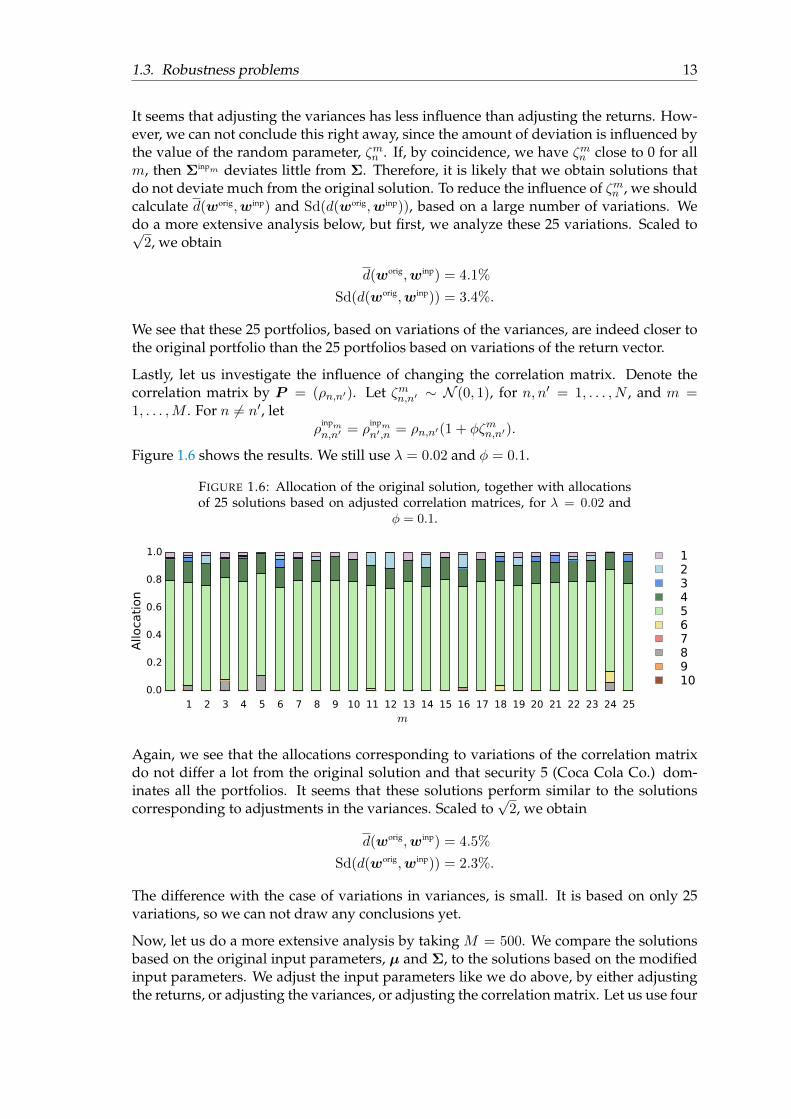
Figure 1.6 shows the results. We still use λ = 0.02 and φ = 0.1.
FIGURE 1.6: Allocation of the original solution, together with allocationsof 25 solutions based on adjusted correlation matrices, for λ = 0.02 and
φ = 0.1.
1 2 3 4 5 6 7 8 9 10 11 12 13 14 15 16 17 18 19 20 21 22 23 24 25m
0.0
0.2
0.4
0.6
0.8
1.0
Allo
cati
on
12345678910
Again, we see that the allocations corresponding to variations of the correlation matrixdo not differ a lot from the original solution and that security 5 (Coca Cola Co.) dom-inates all the portfolios. It seems that these solutions perform similar to the solutionscorresponding to adjustments in the variances. Scaled to
√2, we obtain
d(worig,winp) = 4.5%
Sd(d(worig,winp)) = 2.3%.
The difference with the case of variations in variances, is small. It is based on only 25variations, so we can not draw any conclusions yet.
Now, let us do a more extensive analysis by taking M = 500. We compare the solutionsbased on the original input parameters, µ and Σ, to the solutions based on the modifiedinput parameters. We adjust the input parameters like we do above, by either adjustingthe returns, or adjusting the variances, or adjusting the correlation matrix. Let us use four
14 Chapter 1. Mean-Variance optimization
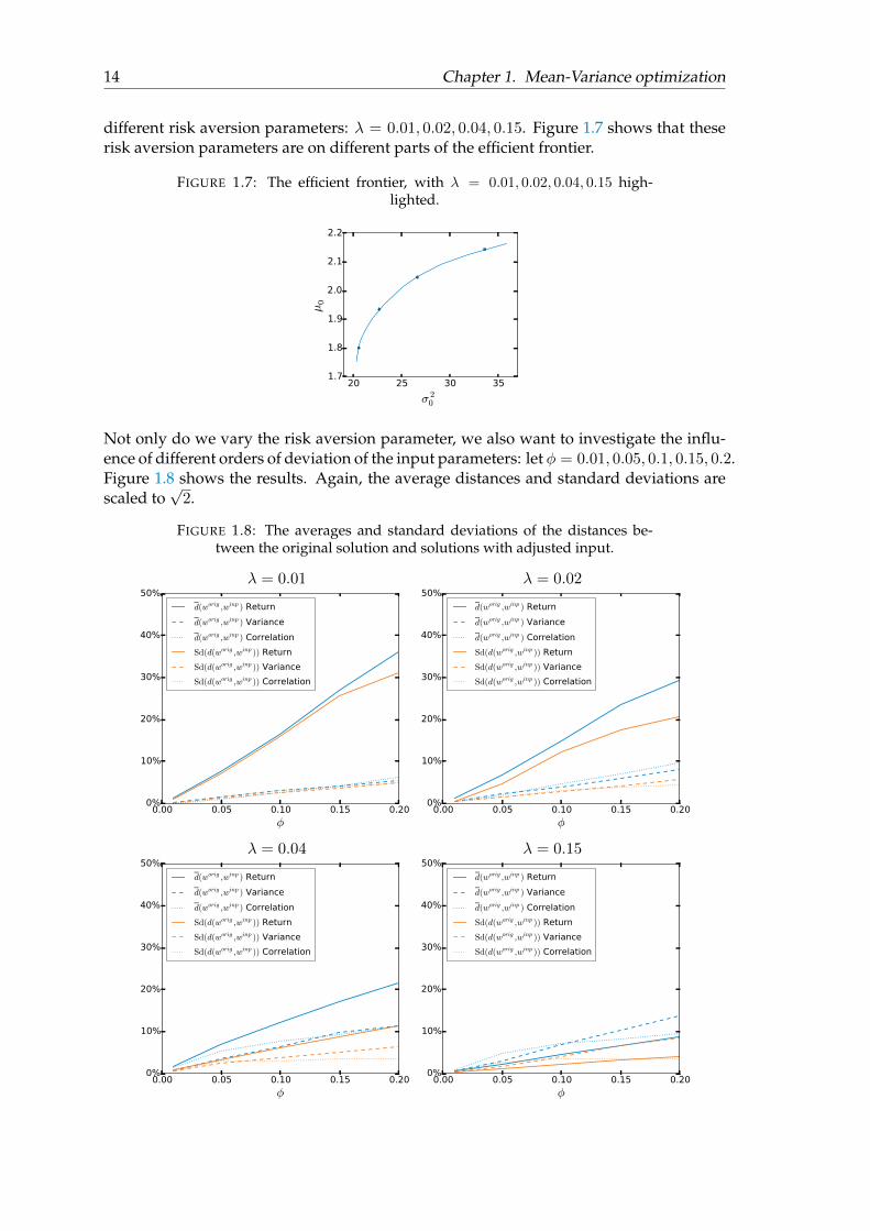
different risk aversion parameters: λ = 0.01, 0.02, 0.04, 0.15. Figure 1.7 shows that theserisk aversion parameters are on different parts of the efficient frontier.
FIGURE 1.7: The efficient frontier, with λ = 0.01, 0.02, 0.04, 0.15 high-lighted.
20 25 30 35
σ 20
1.7
1.8
1.9
2.0
2.1
2.2
µ0
Not only do we vary the risk aversion parameter, we also want to investigate the influ-ence of different orders of deviation of the input parameters: let φ = 0.01, 0.05, 0.1, 0.15, 0.2.Figure 1.8 shows the results. Again, the average distances and standard deviations arescaled to
√2.
FIGURE 1.8: The averages and standard deviations of the distances be-tween the original solution and solutions with adjusted input.
λ = 0.01 λ = 0.02
0.00 0.05 0.10 0.15 0.20
φ
0%
10%
20%
30%
40%
50%
d(worig ,winp ) Return
d(worig ,winp ) Variance
d(worig ,winp ) Correlation
Sd(d(worig ,winp )) Return
Sd(d(worig ,winp )) Variance
Sd(d(worig ,winp )) Correlation
0.00 0.05 0.10 0.15 0.20
φ
0%
10%
20%
30%
40%
50%
d(worig ,winp ) Return
d(worig ,winp ) Variance
d(worig ,winp ) Correlation
Sd(d(worig ,winp )) Return
Sd(d(worig ,winp )) Variance
Sd(d(worig ,winp )) Correlation
λ = 0.04 λ = 0.15
0.00 0.05 0.10 0.15 0.20
φ
0%
10%
20%
30%
40%
50%
d(worig ,winp ) Return
d(worig ,winp ) Variance
d(worig ,winp ) Correlation
Sd(d(worig ,winp )) Return
Sd(d(worig ,winp )) Variance
Sd(d(worig ,winp )) Correlation
0.00 0.05 0.10 0.15 0.20
φ
0%
10%
20%
30%
40%
50%
d(worig ,winp ) Return
d(worig ,winp ) Variance
d(worig ,winp ) Correlation
Sd(d(worig ,winp )) Return
Sd(d(worig ,winp )) Variance
Sd(d(worig ,winp )) Correlation
1.3. Robustness problems 15
We see for all three kind of adjustments that the average distance increases, as the valueof φ increases. This is as expected, because when we have a large order of deviation ofthe input parameters, there is a high probability that some asset class suddenly attainsfavorable features, like a high return in combinations with a low risk. This asset classattains a lot of weight for this iteration and in each iteration this can be another assetclass. Hence, we obtain portfolios that are not robust.
For λ = 0.01, λ = 0.02, and λ = 0.04, we see that d(worig,winp), corresponding to ad-justed returns is biggest and increases faster than the others. This means that in thiscase, adjusting the returns has the biggest impact on the allocations. For λ = 0.15 andφ < 0.10, we see that the average distance of adjusted correlations is slightly bigger thanthe rest, hence, adjusting the correlations and have the biggest effect here. Furthermore,for λ = 0.15 and φ > 0.11, we see that the adjusting the variances has the biggest effecton the allocations.
We can make similar observations when we look at the standard deviations. As opposedto the average distance, we see that the standard deviations do not necessarily get smaller,as the value of λ increases.
An important note is that we do not know whether or not the relation between high riskaversion and low average distance, is a causal relation. We only want to point out thatthe effect can be different for different risk aversion parameters.
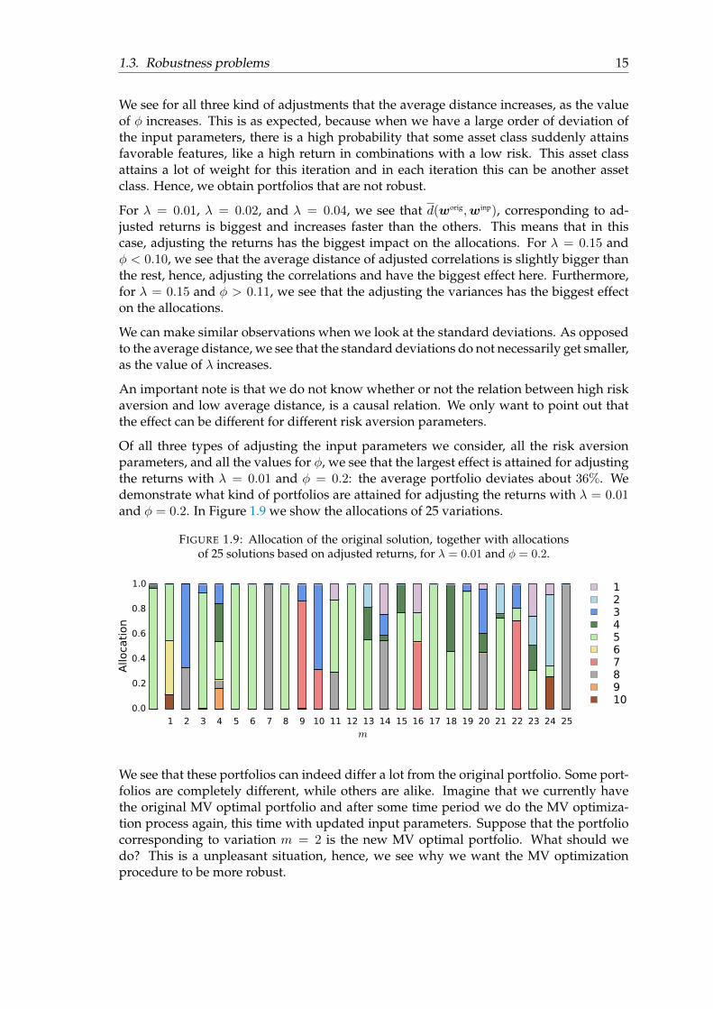
Of all three types of adjusting the input parameters we consider, all the risk aversionparameters, and all the values for φ, we see that the largest effect is attained for adjustingthe returns with λ = 0.01 and φ = 0.2: the average portfolio deviates about 36%. Wedemonstrate what kind of portfolios are attained for adjusting the returns with λ = 0.01and φ = 0.2. In Figure 1.9 we show the allocations of 25 variations.
FIGURE 1.9: Allocation of the original solution, together with allocationsof 25 solutions based on adjusted returns, for λ = 0.01 and φ = 0.2.
1 2 3 4 5 6 7 8 9 10 11 12 13 14 15 16 17 18 19 20 21 22 23 24 25m
0.0
0.2
0.4
0.6
0.8
1.0
Allo
cati
on
12345678910
We see that these portfolios can indeed differ a lot from the original portfolio. Some port-folios are completely different, while others are alike. Imagine that we currently havethe original MV optimal portfolio and after some time period we do the MV optimiza-tion process again, this time with updated input parameters. Suppose that the portfoliocorresponding to variation m = 2 is the new MV optimal portfolio. What should wedo? This is a unpleasant situation, hence, we see why we want the MV optimizationprocedure to be more robust.
16 Chapter 1. Mean-Variance optimization
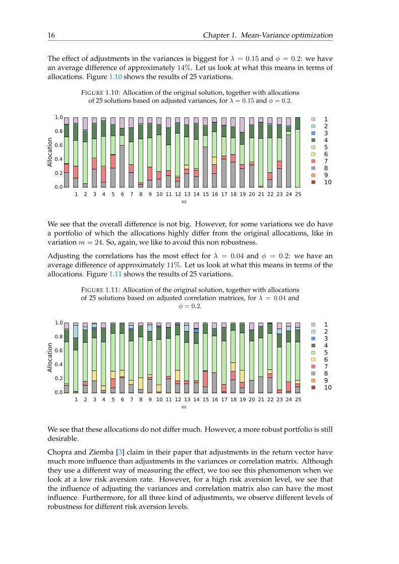
The effect of adjustments in the variances is biggest for λ = 0.15 and φ = 0.2: we havean average difference of approximately 14%. Let us look at what this means in terms ofallocations. Figure 1.10 shows the results of 25 variations.
FIGURE 1.10: Allocation of the original solution, together with allocationsof 25 solutions based on adjusted variances, for λ = 0.15 and φ = 0.2.
1 2 3 4 5 6 7 8 9 10 11 12 13 14 15 16 17 18 19 20 21 22 23 24 25m
0.0
0.2
0.4
0.6
0.8
1.0
Allo
cati
on
12345678910
We see that the overall difference is not big. However, for some variations we do havea portfolio of which the allocations highly differ from the original allocations, like invariation m = 24. So, again, we like to avoid this non robustness.
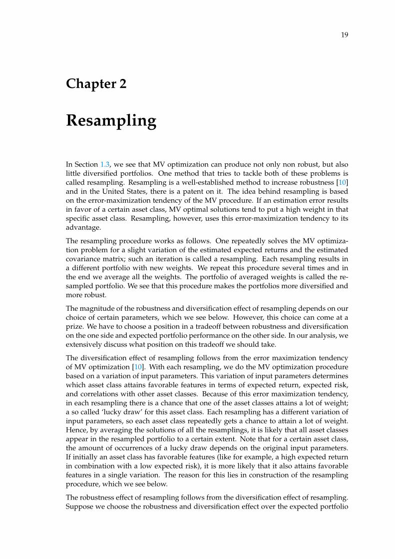
Adjusting the correlations has the most effect for λ = 0.04 and φ = 0.2: we have anaverage difference of approximately 11%. Let us look at what this means in terms of theallocations. Figure 1.11 shows the results of 25 variations.
FIGURE 1.11: Allocation of the original solution, together with allocationsof 25 solutions based on adjusted correlation matrices, for λ = 0.04 and
φ = 0.2.
1 2 3 4 5 6 7 8 9 10 11 12 13 14 15 16 17 18 19 20 21 22 23 24 25m
0.0
0.2
0.4
0.6
0.8
1.0
Allo
cati
on
12345678910
We see that these allocations do not differ much. However, a more robust portfolio is stilldesirable.
Chopra and Ziemba [3] claim in their paper that adjustments in the return vector havemuch more influence than adjustments in the variances or correlation matrix. Althoughthey use a different way of measuring the effect, we too see this phenomenon when welook at a low risk aversion rate. However, for a high risk aversion level, we see thatthe influence of adjusting the variances and correlation matrix also can have the mostinfluence. Furthermore, for all three kind of adjustments, we observe different levels ofrobustness for different risk aversion levels.

1.3. Robustness problems 17
Not only use Chopra and Ziemba another measurement tool, but they also look at onlyone risk aversion parameter: λ = 0.04. Hence, we can not properly compare our results totheirs. Nevertheless, it has become clear that using adjusted input parameters can resultin MV optimal portfolios that highly differ in terms of allocations.
1.3.1.1 Conclusion
A small change in any of the input parameters can result in a big change in allocations ofthe MV optimal portfolios. For this reason, we search for more robust portfolios.
Although Chopra and Ziemba claim that the effect of adjustments in the returns havethe most effect on the allocations, we know this is not always the case. It all dependson the order of deviation of the input parameters and on the value of the risk aversionparameter.

19
Chapter 2
Resampling
In Section 1.3, we see that MV optimization can produce not only non robust, but alsolittle diversified portfolios. One method that tries to tackle both of these problems iscalled resampling. Resampling is a well-established method to increase robustness [10]and in the United States, there is a patent on it. The idea behind resampling is basedon the error-maximization tendency of the MV procedure. If an estimation error resultsin favor of a certain asset class, MV optimal solutions tend to put a high weight in thatspecific asset class. Resampling, however, uses this error-maximization tendency to itsadvantage.
The resampling procedure works as follows. One repeatedly solves the MV optimiza-tion problem for a slight variation of the estimated expected returns and the estimatedcovariance matrix; such an iteration is called a resampling. Each resampling results ina different portfolio with new weights. We repeat this procedure several times and inthe end we average all the weights. The portfolio of averaged weights is called the re-sampled portfolio. We see that this procedure makes the portfolios more diversified andmore robust.
The magnitude of the robustness and diversification effect of resampling depends on ourchoice of certain parameters, which we see below. However, this choice can come at aprize. We have to choose a position in a tradeoff between robustness and diversificationon the one side and expected portfolio performance on the other side. In our analysis, weextensively discuss what position on this tradeoff we should take.
The diversification effect of resampling follows from the error maximization tendencyof MV optimization [10]. With each resampling, we do the MV optimization procedurebased on a variation of input parameters. This variation of input parameters determineswhich asset class attains favorable features in terms of expected return, expected risk,and correlations with other asset classes. Because of this error maximization tendency,in each resampling there is a chance that one of the asset classes attains a lot of weight;a so called ‘lucky draw’ for this asset class. Each resampling has a different variation ofinput parameters, so each asset class repeatedly gets a chance to attain a lot of weight.Hence, by averaging the solutions of all the resamplings, it is likely that all asset classesappear in the resampled portfolio to a certain extent. Note that for a certain asset class,the amount of occurrences of a lucky draw depends on the original input parameters.If initially an asset class has favorable features (like for example, a high expected returnin combination with a low expected risk), it is more likely that it also attains favorablefeatures in a single variation. The reason for this lies in construction of the resamplingprocedure, which we see below.
The robustness effect of resampling follows from the diversification effect of resampling.Suppose we choose the robustness and diversification effect over the expected portfolio
20 Chapter 2. Resampling
performance, then the resampled portfolio that we attain is well diversified, due to rea-sons we explain above. Suppose it turns out that the original input parameters are notcorrect and we do the resampling procedure again, this time with the new, better inputparameters, then, we have a high probability that the newly attained portfolio is also welldiversified (provided that we remain to be on the robustness and diversification side ofthe tradeoff). We now have two well diversified portfolios: one based on the old inputparameters and one based on the new input parameters. We see that the difference be-tween the two portfolios is small and thus is the resampled portfolio, based on the initialinput, robust.
The last important property of resampling is that the resampled frontier, i.e., the frontierobtained by doing the resampling procedure for different risk/return levels, can containconvex parts. In Theorem 2.2.2, we show that for a simplified version of the resamplingprocedure, the probability of convex parts in the resampled frontier converges to zero, asthe number of resamplings goes to infinity.
2.1 Formulation
Unless stated otherwise, we assume that we are not allowed to go short. We define theresampling procedure for the risk aversion formulation; this means that we average thesolutions that correspond to the same risk aversion parameter. One could also choose todo the resampling procedure based on the minimum risk formulation. That is, do theresampling procedure and average the solutions that correspond to the same required re-turn. Or, one could choose to do the resampling procedure based on the maximum returnformulation, i.e., do the resampling procedure and average the solutions that correspondto the same level of risk.
We argue that doing the resampling procedure based on the risk aversion formulation isthe best choice. To see this, consider the case in which we average per required expectedrisk and our required expected risk, σ20 , is as small as possible. Then, we have the pos-sibility that in a resampling, the variation of input parameters is such that an expectedportfolio risk of σ20 can not be attained. When we average all solutions of the resamplings,we are forced to include portfolios with a higher expected risk level, which initially wasnot our intention.
Suppose we do the resampling procedure for some fixed expected required return (notnecessarily the smallest possible) and suppose that for some resampling, the variation ofinput parameters is such that the obtained expected portfolio risk is large. Then, maybewe are not willing to take such a big risk but we want to adjust the expected return we re-quire. This is not possible when we average per fixed expected required return. However,when we average per risk aversion parameter, the return and risk level automatically ad-justs to the correct equilibrium. Hence, the portfolios we average are all portfolios that fitour risk aversion appetite.
For risk aversion parameter λ ≥ 0, recall from Section 1.1 the risk aversion formulationof MV optimization:
minw
λwᵀΣw −wᵀµ, subject to wᵀ1 = 1, w ≥ 0.
2.1. Formulation 21
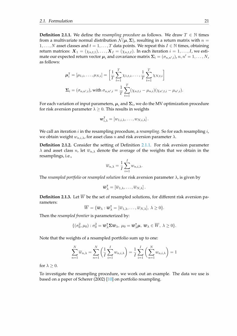
Definition 2.1.1. We define the resampling procedure as follows. We draw T ∈ N timesfrom a multivariate normal distribution N (µ,Σ), resulting in a return matrix with n =1, . . . , N asset classes and t = 1, . . . , T data points. We repeat this I ∈ N times, obtainingreturn matrices: X1 = (χn,t,1), . . . ,XI = (χn,t,I). In each iteration i = 1, . . . , I , we esti-mate our expected return vector µi and covariance matrix Σi = (σn,n′,i), n, n′ = 1, . . . , N ,as follows:
µᵀi = [µ1,i, . . . , µN,i] =
[1
T
T∑t=1
χ1,t,i, . . . ,1
T
T∑t=1
χN,t,i
]
Σi = (σn,n′,i), with σn,n′,i =1
T
T∑t=1
(χn,t,i − µn,i)(χn′,t,i − µn′,i).
For each variation of input parameters, µi and Σi, we do the MV optimization procedurefor risk aversion parameter λ ≥ 0. This results in weights
wᵀi,λ = [w1,i,λ, . . . , wN,i,λ] .
We call an iteration i in the resampling procedure, a resampling. So for each resampling i,we obtain weight wn,i,λ, for asset class n and risk aversion parameter λ.
Definition 2.1.2. Consider the setting of Definition 2.1.1. For risk aversion parameterλ and asset class n, let wn,λ denote the average of the weights that we obtain in theresamplings, i.e.,
wn,λ =1
I
I∑i=1
wn,i,λ.
The resampled portfolio or resampled solution for risk aversion parameter λ, is given by
wᵀλ = [w1,λ, . . . , wN,λ] .
Definition 2.1.3. Let W be the set of resampled solutions, for different risk aversion pa-rameters:
W = {wλ : wᵀλ = [w1,λ, . . . , wN,λ], λ ≥ 0}.
Then the resampled frontier is parameterized by:
{(σ20, µ0) : σ20 = wᵀλΣwλ, µ0 = wᵀ
λµ, wλ ∈W, λ ≥ 0}.
Note that the weights of a resampled portfolio sum up to one:
N∑n=1
wn,λ =
N∑n=1
(1
I
I∑i=1
wn,i,λ
)=
1
I
I∑i=1
( N∑n=1
wn,i,λ
)= 1
for λ ≥ 0.
To investigate the resampling procedure, we work out an example. The data we use isbased on a paper of Scherer (2002) [10] on portfolio resampling.
22 Chapter 2. Resampling
2.2 Example
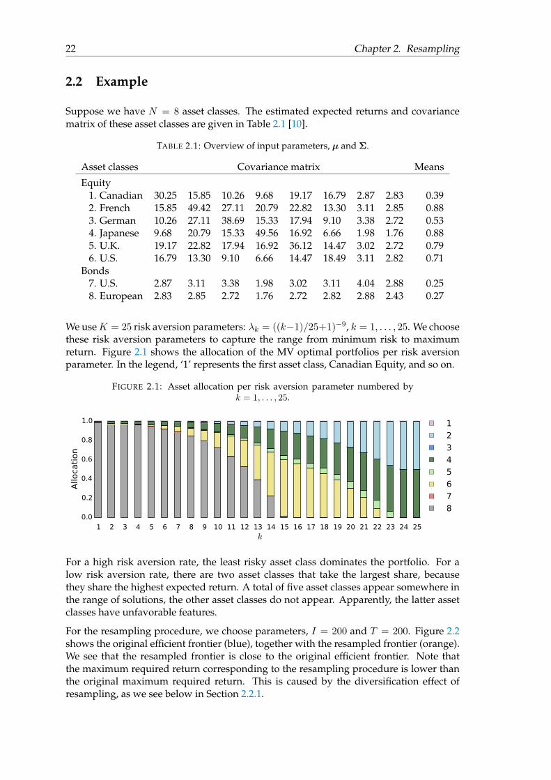
Suppose we have N = 8 asset classes. The estimated expected returns and covariancematrix of these asset classes are given in Table 2.1 [10].
TABLE 2.1: Overview of input parameters, µ and Σ.
Asset classes Covariance matrix Means
Equity1. Canadian 30.25 15.85 10.26 9.68 19.17 16.79 2.87 2.83 0.392. French 15.85 49.42 27.11 20.79 22.82 13.30 3.11 2.85 0.883. German 10.26 27.11 38.69 15.33 17.94 9.10 3.38 2.72 0.534. Japanese 9.68 20.79 15.33 49.56 16.92 6.66 1.98 1.76 0.885. U.K. 19.17 22.82 17.94 16.92 36.12 14.47 3.02 2.72 0.796. U.S. 16.79 13.30 9.10 6.66 14.47 18.49 3.11 2.82 0.71
Bonds7. U.S. 2.87 3.11 3.38 1.98 3.02 3.11 4.04 2.88 0.258. European 2.83 2.85 2.72 1.76 2.72 2.82 2.88 2.43 0.27
We useK = 25 risk aversion parameters: λk = ((k−1)/25+1)−9, k = 1, . . . , 25. We choosethese risk aversion parameters to capture the range from minimum risk to maximumreturn. Figure 2.1 shows the allocation of the MV optimal portfolios per risk aversionparameter. In the legend, ‘1’ represents the first asset class, Canadian Equity, and so on.
FIGURE 2.1: Asset allocation per risk aversion parameter numbered byk = 1, . . . , 25.
1 2 3 4 5 6 7 8 9 10 11 12 13 14 15 16 17 18 19 20 21 22 23 24 25k
0.0
0.2
0.4
0.6
0.8
1.0
Allo
cati
on
1
2
3
4
5
6
7
8
For a high risk aversion rate, the least risky asset class dominates the portfolio. For alow risk aversion rate, there are two asset classes that take the largest share, becausethey share the highest expected return. A total of five asset classes appear somewhere inthe range of solutions, the other asset classes do not appear. Apparently, the latter assetclasses have unfavorable features.
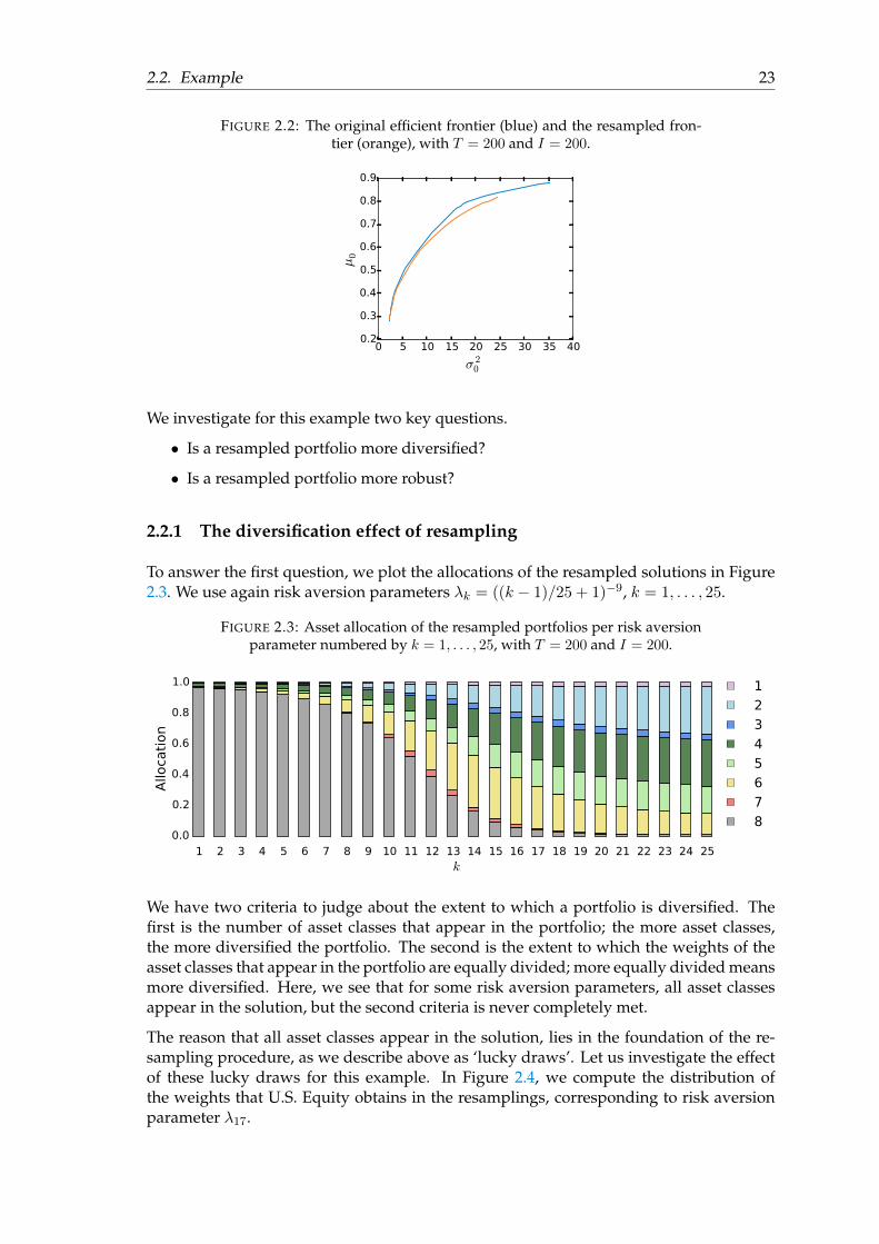
For the resampling procedure, we choose parameters, I = 200 and T = 200. Figure 2.2shows the original efficient frontier (blue), together with the resampled frontier (orange).We see that the resampled frontier is close to the original efficient frontier. Note thatthe maximum required return corresponding to the resampling procedure is lower thanthe original maximum required return. This is caused by the diversification effect ofresampling, as we see below in Section 2.2.1.
2.2. Example 23
FIGURE 2.2: The original efficient frontier (blue) and the resampled fron-tier (orange), with T = 200 and I = 200.
0 5 10 15 20 25 30 35 40
σ 20
0.2
0.3
0.4
0.5
0.6
0.7
0.8
0.9
µ0
We investigate for this example two key questions.
• Is a resampled portfolio more diversified?
• Is a resampled portfolio more robust?
2.2.1 The diversification effect of resampling
To answer the first question, we plot the allocations of the resampled solutions in Figure2.3. We use again risk aversion parameters λk = ((k − 1)/25 + 1)−9, k = 1, . . . , 25.
FIGURE 2.3: Asset allocation of the resampled portfolios per risk aversionparameter numbered by k = 1, . . . , 25, with T = 200 and I = 200.
1 2 3 4 5 6 7 8 9 10 11 12 13 14 15 16 17 18 19 20 21 22 23 24 25k
0.0
0.2
0.4
0.6
0.8
1.0
Allo
cati
on
1
2
3
4
5
6
7
8
We have two criteria to judge about the extent to which a portfolio is diversified. Thefirst is the number of asset classes that appear in the portfolio; the more asset classes,the more diversified the portfolio. The second is the extent to which the weights of theasset classes that appear in the portfolio are equally divided; more equally divided meansmore diversified. Here, we see that for some risk aversion parameters, all asset classesappear in the solution, but the second criteria is never completely met.
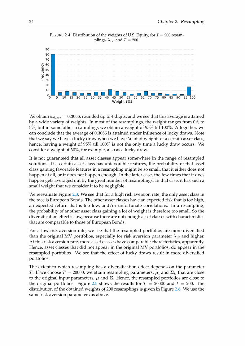
The reason that all asset classes appear in the solution, lies in the foundation of the re-sampling procedure, as we describe above as ‘lucky draws’. Let us investigate the effectof these lucky draws for this example. In Figure 2.4, we compute the distribution ofthe weights that U.S. Equity obtains in the resamplings, corresponding to risk aversionparameter λ17.
24 Chapter 2. Resampling
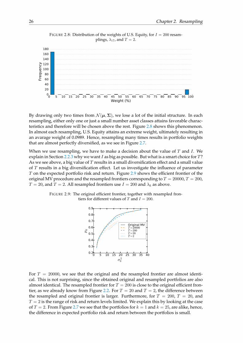
FIGURE 2.4: Distribution of the weights of U.S. Equity, for I = 200 resam-plings, λ17, and T = 200.
0 5 10 15 20 25 30 35 40 45 50 55 60 65 70 75 80 85 90 95 100Weight (%)
0
10
20
30
40
50
60
70
80
90
Frequency
We obtainw6,λ17 = 0.3066, rounded up to 4 digits, and we see that this average is attainedby a wide variety of weights. In most of the resamplings, the weight ranges from 0% to5%, but in some other resamplings we obtain a weight of 95% till 100%. Altogether, wecan conclude that the average of 0.3066 is attained under influence of lucky draws. Notethat we say we have a lucky draw when we have ‘a lot of weight’ of a certain asset class,hence, having a weight of 95% till 100% is not the only time a lucky draw occurs. Weconsider a weight of 50%, for example, also as a lucky draw.
It is not guaranteed that all asset classes appear somewhere in the range of resampledsolutions. If a certain asset class has unfavorable features, the probability of that assetclass gaining favorable features in a resampling might be so small, that it either does nothappen at all, or it does not happen enough. In the latter case, the few times that it doeshappen gets averaged out by the great number of resamplings. In that case, it has such asmall weight that we consider it to be negligible.
We reevaluate Figure 2.3. We see that for a high risk aversion rate, the only asset class inthe race is European Bonds. The other asset classes have an expected risk that is too high,an expected return that is too low, and/or unfortunate correlations. In a resampling,the probability of another asset class gaining a lot of weight is therefore too small. So thediversification effect is low, because there are not enough asset classes with characteristicsthat are comparable to those of European Bonds.
For a low risk aversion rate, we see that the resampled portfolios are more diversifiedthan the original MV portfolios, especially for risk aversion parameter λ12 and higher.At this risk aversion rate, more asset classes have comparable characteristics, apparently.Hence, asset classes that did not appear in the original MV portfolios, do appear in theresampled portfolios. We see that the effect of lucky draws result in more diversifiedportfolios.
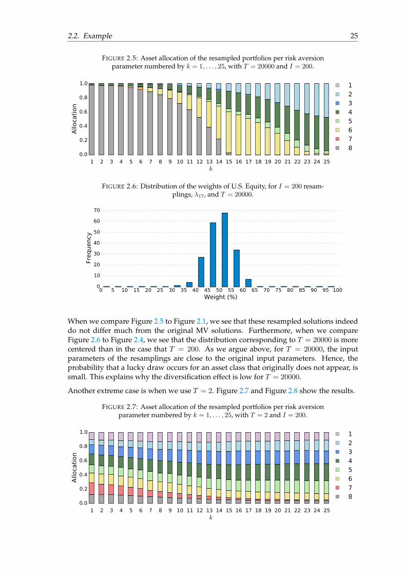
The extent to which resampling has a diversification effect depends on the parameterT . If we choose T = 20000, we attain resampling parameters, µi and Σi, that are closeto the original input parameters, µ and Σ. Hence, the resampled portfolios are close tothe original portfolios. Figure 2.5 shows the results for T = 20000 and I = 200. Thedistribution of the obtained weights of 200 resamplings is given in Figure 2.6. We use thesame risk aversion parameters as above.
2.2. Example 25
FIGURE 2.5: Asset allocation of the resampled portfolios per risk aversionparameter numbered by k = 1, . . . , 25, with T = 20000 and I = 200.
1 2 3 4 5 6 7 8 9 10 11 12 13 14 15 16 17 18 19 20 21 22 23 24 25k
0.0
0.2
0.4
0.6
0.8
1.0
Allo
cati
on
1
2
3
4
5
6
7
8
FIGURE 2.6: Distribution of the weights of U.S. Equity, for I = 200 resam-plings, λ17, and T = 20000.
0 5 10 15 20 25 30 35 40 45 50 55 60 65 70 75 80 85 90 95 100Weight (%)
0
10
20
30
40
50
60
70
Frequency
When we compare Figure 2.5 to Figure 2.1, we see that these resampled solutions indeeddo not differ much from the original MV solutions. Furthermore, when we compareFigure 2.6 to Figure 2.4, we see that the distribution corresponding to T = 20000 is morecentered than in the case that T = 200. As we argue above, for T = 20000, the inputparameters of the resamplings are close to the original input parameters. Hence, theprobability that a lucky draw occurs for an asset class that originally does not appear, issmall. This explains why the diversification effect is low for T = 20000.
Another extreme case is when we use T = 2. Figure 2.7 and Figure 2.8 show the results.
FIGURE 2.7: Asset allocation of the resampled portfolios per risk aversionparameter numbered by k = 1, . . . , 25, with T = 2 and I = 200.
1 2 3 4 5 6 7 8 9 10 11 12 13 14 15 16 17 18 19 20 21 22 23 24 25k
0.0
0.2
0.4
0.6
0.8
1.0
Allo
cati
on
1
2
3
4
5
6
7
8
26 Chapter 2. Resampling
FIGURE 2.8: Distribution of the weights of U.S. Equity, for I = 200 resam-plings, λ17, and T = 2.
0 5 10 15 20 25 30 35 40 45 50 55 60 65 70 75 80 85 90 95 100Weight (%)
0
20
40
60
80
100
120
140
160
180
Frequency
By drawing only two times from N (µ,Σ), we lose a lot of the initial structure. In eachresampling, either only one or just a small number asset classes attains favorable charac-teristics and therefore will be chosen above the rest. Figure 2.8 shows this phenomenon.In almost each resampling, U.S. Equity attains an extreme weight, ultimately resulting inan avarage weight of 0.0989. Hence, resampling many times results in portfolio weightsthat are almost perfectly diversified, as we see in Figure 2.7.
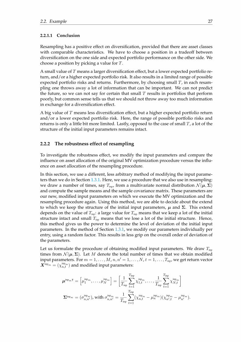
When we use resampling, we have to make a decision about the value of T and I . Weexplain in Section 2.2.3 why we want I as big as possible. But what is a smart choice for T ?As we see above, a big value of T results in a small diversification effect and a small valueof T results in a big diversification effect. Let us investigate the influence of parameterT on the expected portfolio risk and return. Figure 2.9 shows the efficient frontier of theoriginal MV procedure and the resampled frontiers corresponding to T = 20000, T = 200,T = 20, and T = 2. All resampled frontiers use I = 200 and λk as above.
FIGURE 2.9: The original efficient frontier, together with resampled fron-tiers for different values of T and I = 200.
0 5 10 15 20 25 30 35 40
σ 20
0.2
0.3
0.4
0.5
0.6
0.7
0.8
0.9
µ0
Original MVT=20000T=200T=20T=2
For T = 20000, we see that the original and the resampled frontier are almost identi-cal. This is not surprising, since the obtained original and resampled portfolios are alsoalmost identical. The resampled frontier for T = 200 is close to the original efficient fron-tier, as we already know from Figure 2.2. For T = 20 and T = 2, the difference betweenthe resampled and original frontier is larger. Furthermore, for T = 200, T = 20, andT = 2 is the range of risk and return levels limited. We explain this by looking at the caseof T = 2. From Figure 2.7 we see that the portfolios for k = 1 and k = 25, are alike, hence,the difference in expected portfolio risk and return between the portfolios is small.
2.2. Example 27
2.2.1.1 Conclusion
Resampling has a positive effect on diversification, provided that there are asset classeswith comparable characteristics. We have to choose a position in a tradeoff betweendiversification on the one side and expected portfolio performance on the other side. Wechoose a position by picking a value for T .
A small value of T means a larger diversification effect, but a lower expected portfolio re-turn, and/or a higher expected portfolio risk. It also results in a limited range of possibleexpected portfolio risks and returns. Furthermore, by choosing small T , in each resam-pling one throws away a lot of information that can be important. We can not predictthe future, so we can not say for certain that small T results in portfolios that performpoorly, but common sense tells us that we should not throw away too much informationin exchange for a diversification effect.
A big value of T means less diversification effect, but a higher expected portfolio returnand/or a lower expected portfolio risk. Here, the range of possible portfolio risks andreturns is only a little bit more limited. Lastly, opposed to the case of small T , a lot of thestructure of the initial input parameters remains intact.
2.2.2 The robustness effect of resampling
To investigate the robustness effect, we modify the input parameters and compare theinfluence on asset allocation of the original MV optimization procedure versus the influ-ence on asset allocation of the resampling procedure.
In this section, we use a different, less arbitrary method of modifying the input parame-ters than we do in Section 1.3.1. Here, we use a procedure that we also use in resampling:we draw a number of times, say Tinp, from a multivariate normal distribution N (µ,Σ)and compute the sample means and the sample covariance matrix. These parameters areour new, modified input parameters on which we execute the MV optimization and theresampling procedure again. Using this method, we are able to decide about the extendto which we keep the structure of the initial input parameters, µ and Σ. This extenddepends on the value of Tinp: a large value for Tinp means that we keep a lot of the initialstructure intact and small Tinp means that we lose a lot of the initial structure. Hence,this method gives us the power to determine the level of deviation of the initial inputparameters. In the method of Section 1.3.1, we modify our parameters individually perentry, using a random factor. This results in less grip on the overall order of deviation ofthe parameters.
Let us formulate the procedure of obtaining modified input parameters. We draw Tinp
times from N (µ,Σ). Let M denote the total number of times that we obtain modifiedinput parameters. For m = 1, . . . ,M , n, n′ = 1, . . . , N , t = 1, . . . , Tinp, we get return vectorX inpm = (χ
inpmn,t ) and modified input parameters:
µinpmᵀ =[µ
inpm1 , . . . , µ
inpmN
]=
[1
Tinp
Tinp∑t=1
χinpm1,t , . . . ,
1
Tinp
Tinp∑t=1
χinpmN,t
]
Σinpm = (σinpmn,n′ ), with σinpm
n,n′ =1
Tinp
Tinp∑t=1
(χinpmn,t − µ
inpmn )(χ
inpmn′,t − µ
inpmn′ ).
28 Chapter 2. Resampling
Based on the original and modified input parameters, we execute the MV optimizationmethod and the resampling method. Note that in a resampling i = 1, . . . , I , we againdraw a number of times from a normal distribution: T times from N (µinpm ,Σinpm). Thisresults in a return vector X inpm
i = (χinpmn,t,i), t = 1, . . . , T . For variation m and resampling i,
we obtain parameters:
µinpmᵀi =
[µ
inpm1,i , . . . , µ
inpmN,i
]=
[1
T
T∑t=1
χm1,t,i, . . . ,1
T
T∑t=1
χmN,t,i
]
Σinpmi = (σ
inpmn,n′,i), with σinpm
n,n′,i =1
T
T∑t=1
(χmn,t,i − µinpmn,i )(χmn′,t,i − µ
inpmn′,i ).
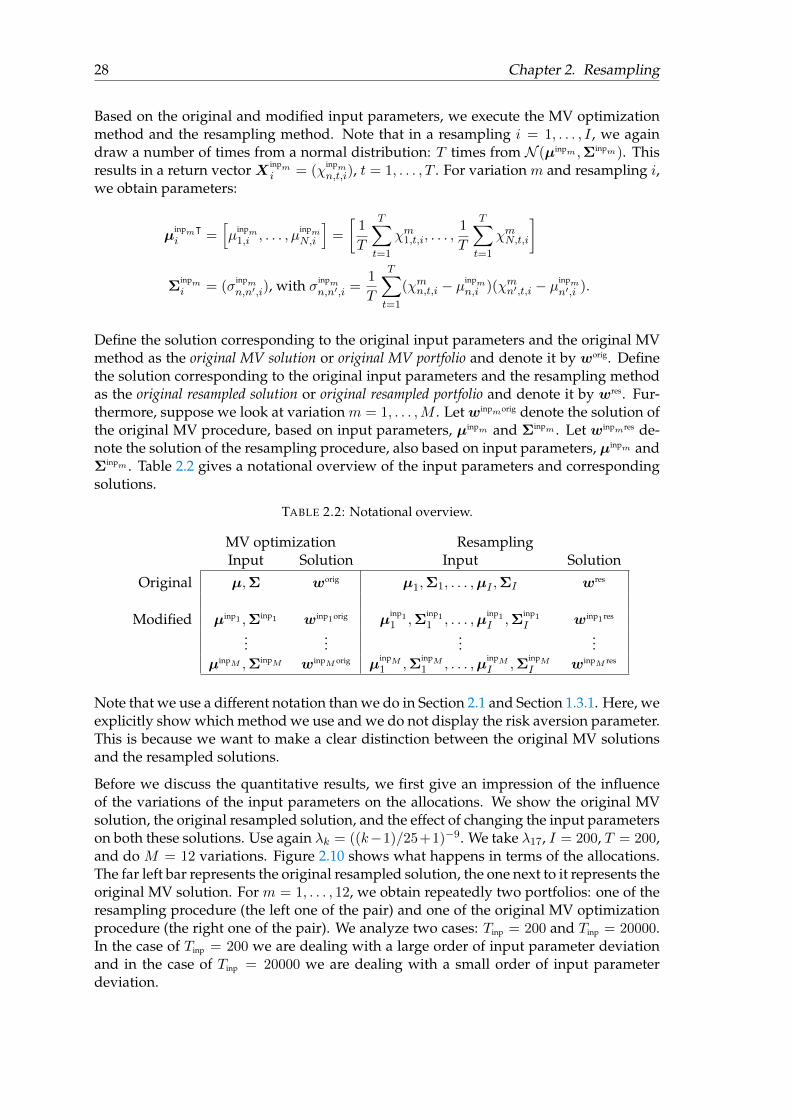
Define the solution corresponding to the original input parameters and the original MVmethod as the original MV solution or original MV portfolio and denote it by worig. Definethe solution corresponding to the original input parameters and the resampling methodas the original resampled solution or original resampled portfolio and denote it by wres. Fur-thermore, suppose we look at variation m = 1, . . . ,M . Letwinpmorig denote the solution ofthe original MV procedure, based on input parameters, µinpm and Σinpm . Let winpmres de-note the solution of the resampling procedure, also based on input parameters, µinpm andΣinpm . Table 2.2 gives a notational overview of the input parameters and correspondingsolutions.
TABLE 2.2: Notational overview.
MV optimization ResamplingInput Solution Input Solution
Original µ,Σ worig µ1,Σ1, . . . ,µI ,ΣI wres
Modified µinp1 ,Σinp1 winp1orig µinp11 ,Σ
inp11 , . . . ,µ
inp1I ,Σ
inp1I winp1res
......
......
µinpM ,ΣinpM winpM orig µinpM1 ,Σ
inpM1 , . . . ,µ
inpMI ,Σ
inpMI winpM res
Note that we use a different notation than we do in Section 2.1 and Section 1.3.1. Here, weexplicitly show which method we use and we do not display the risk aversion parameter.This is because we want to make a clear distinction between the original MV solutionsand the resampled solutions.
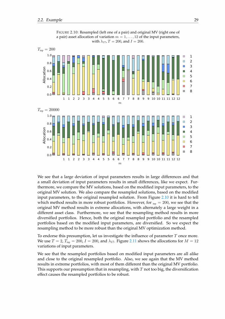
Before we discuss the quantitative results, we first give an impression of the influenceof the variations of the input parameters on the allocations. We show the original MVsolution, the original resampled solution, and the effect of changing the input parameterson both these solutions. Use again λk = ((k−1)/25+1)−9. We take λ17, I = 200, T = 200,and do M = 12 variations. Figure 2.10 shows what happens in terms of the allocations.The far left bar represents the original resampled solution, the one next to it represents theoriginal MV solution. For m = 1, . . . , 12, we obtain repeatedly two portfolios: one of theresampling procedure (the left one of the pair) and one of the original MV optimizationprocedure (the right one of the pair). We analyze two cases: Tinp = 200 and Tinp = 20000.In the case of Tinp = 200 we are dealing with a large order of input parameter deviationand in the case of Tinp = 20000 we are dealing with a small order of input parameterdeviation.
2.2. Example 29
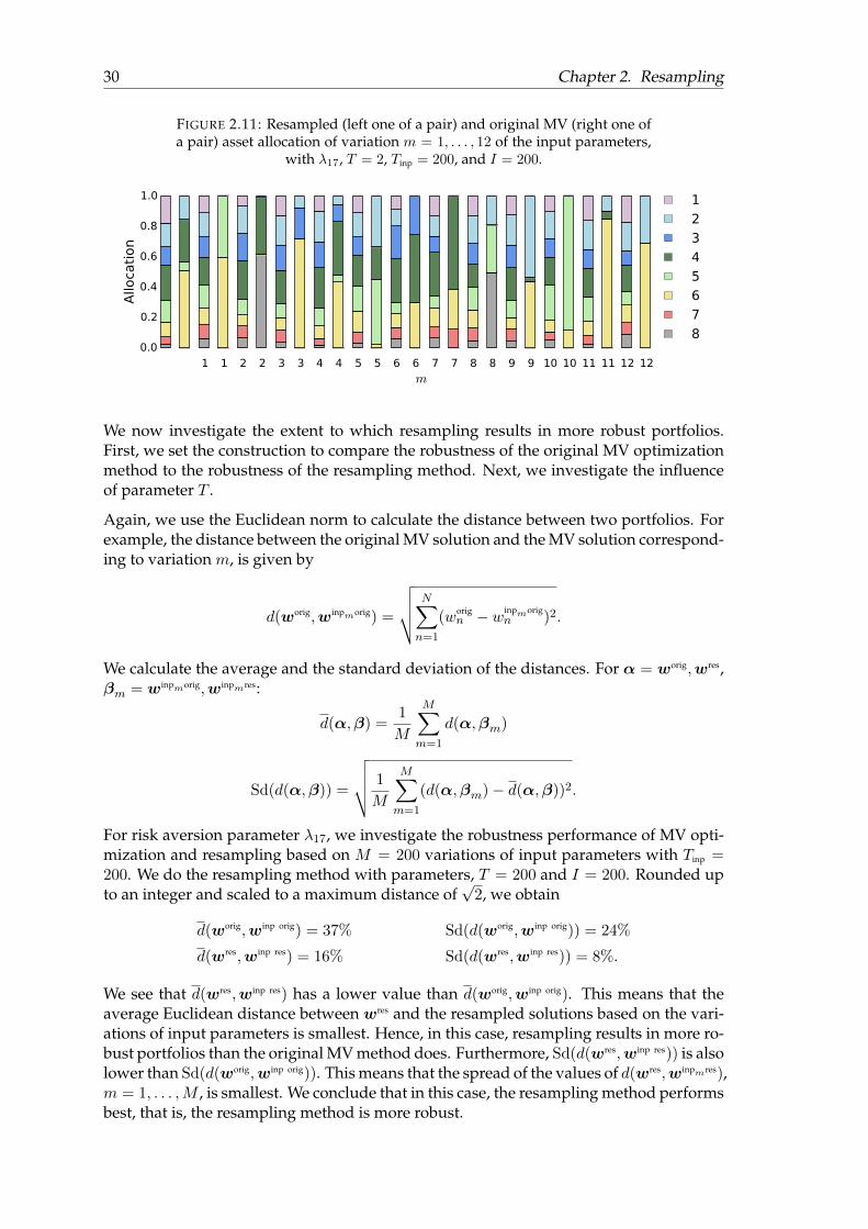
FIGURE 2.10: Resampled (left one of a pair) and original MV (right one ofa pair) asset allocation of variation m = 1, . . . , 12 of the input parameters,
with λ17, T = 200, and I = 200.
Tinp = 200
1 1 2 2 3 3 4 4 5 5 6 6 7 7 8 8 9 9 10 10 11 11 12 12m
0.0
0.2
0.4
0.6
0.8
1.0
Allo
cati
on
1
2
3
4
5
6
7
8
Tinp = 20000
1 1 2 2 3 3 4 4 5 5 6 6 7 7 8 8 9 9 10 10 11 11 12 12m
0.0
0.2
0.4
0.6
0.8
1.0
Allo
cati
on
1
2
3
4
5
6
7
8
We see that a large deviation of input parameters results in large differences and thata small deviation of input parameters results in small differences, like we expect. Fur-thermore, we compare the MV solutions, based on the modified input parameters, to theoriginal MV solution. We also compare the resampled solutions, based on the modifiedinput parameters, to the original resampled solution. From Figure 2.10 it is hard to tellwhich method results in more robust portfolios. However, for inp = 200, we see that theoriginal MV method results in extreme allocations, with alternately a large weight in adifferent asset class. Furthermore, we see that the resampling method results in morediversified portfolios. Hence, both the original resampled portfolio and the resampledportfolios based on the modified input parameters, are diversified. So we expect theresampling method to be more robust than the original MV optimization method.
To endorse this presumption, let us investigate the influence of parameter T once more.We use T = 2, Tinp = 200, I = 200, and λ17. Figure 2.11 shows the allocations for M = 12variations of input parameters.
We see that the resampled portfolios based on modified input parameters are all alikeand close to the original resampled portfolio. Also, we see again that the MV methodresults in extreme portfolios, with most of them different than the original MV portfolio.This supports our presumption that in resampling, with T not too big, the diversificationeffect causes the resampled portfolios to be robust.
30 Chapter 2. Resampling
FIGURE 2.11: Resampled (left one of a pair) and original MV (right one ofa pair) asset allocation of variation m = 1, . . . , 12 of the input parameters,
with λ17, T = 2, Tinp = 200, and I = 200.
1 1 2 2 3 3 4 4 5 5 6 6 7 7 8 8 9 9 10 10 11 11 12 12m
0.0
0.2
0.4
0.6
0.8
1.0
Allo
cati
on
1
2
3
4
5
6
7
8
We now investigate the extent to which resampling results in more robust portfolios.First, we set the construction to compare the robustness of the original MV optimizationmethod to the robustness of the resampling method. Next, we investigate the influenceof parameter T .
Again, we use the Euclidean norm to calculate the distance between two portfolios. Forexample, the distance between the original MV solution and the MV solution correspond-ing to variation m, is given by
d(worig,winpmorig) =
√√√√ N∑n=1
(worign − winpmorig
n )2.
We calculate the average and the standard deviation of the distances. For α = worig,wres,βm = winpmorig,winpmres:
d(α,β) =1
M
M∑m=1
d(α,βm)
Sd(d(α,β)) =
√√√√ 1
M
M∑m=1
(d(α,βm)− d(α,β))2.
For risk aversion parameter λ17, we investigate the robustness performance of MV opti-mization and resampling based on M = 200 variations of input parameters with Tinp =200. We do the resampling method with parameters, T = 200 and I = 200. Rounded upto an integer and scaled to a maximum distance of
√2, we obtain
d(worig,winp orig) = 37% Sd(d(worig,winp orig)) = 24%
d(wres,winp res) = 16% Sd(d(wres,winp res)) = 8%.
We see that d(wres,winp res) has a lower value than d(worig,winp orig). This means that theaverage Euclidean distance between wres and the resampled solutions based on the vari-ations of input parameters is smallest. Hence, in this case, resampling results in more ro-bust portfolios than the original MV method does. Furthermore, Sd(d(wres,winp res)) is alsolower than Sd(d(worig,winp orig)). This means that the spread of the values of d(wres,winpmres),m = 1, . . . ,M , is smallest. We conclude that in this case, the resampling method performsbest, that is, the resampling method is more robust.
2.2. Example 31
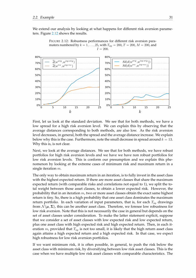
We extend our analysis by looking at what happens for different risk aversion parame-ters. Figure 2.12 shows the results.
FIGURE 2.12: Robustness performances for different risk aversion para-maters numbered by k = 1, . . . , 25, with Tinp = 200, T = 200, M = 200, and
I = 200.
0 5 10 15 20 25
k
0%
10%
20%
30%
40%
50%
60%
70%
80%
d(worig ,winp orig )
d(wres ,winp res )
0 5 10 15 20 25
k
0%
10%
20%
30%
40%
50%
60%
70%
80%
Sd(d(worig ,winp orig ))Sd(d(wres ,winp res ))
First, let us look at the standard deviation. We see that for both methods, we have alow spread for a high risk aversion level. We can explain this by observing that theaverage distances corresponding to both methods, are also low. As the risk aversionlevel decreases, in general, both the spread and the average distance increase. We explainbelow why this is the case. Furthermore, note the small decrease in spread around k = 13.Why this is, is not clear.
Next, we look at the average distances. We see that for both methods, we have robustportfolios for high risk aversion levels and we have we have non robust portfolios forlow risk aversion levels. This is conform our presumption and we explain this phe-nomenon by looking at the extreme cases of minimum risk and maximum return in asingle iteration m.
The only way to obtain maximum return in an iteration, is to fully invest in the asset classwith the highest expected return. If there are more asset classes that share the maximumexpected return (with comparable risks and correlations not equal to 1), we split the to-tal weight between those asset classes, to obtain a lower expected risk. However, theprobability that in an iteration m, two or more asset classes obtain the exact same highestreturn is tiny. So, there is a high probability that one asset class dominates the maximumreturn portfolio. In each variation of input parameters, that is, for each Tinp drawingsfrom N (µ,Σ), this can be another asset class. Therefore, we foresee low robustness forlow risk aversion. Note that this is not necessarily the case in general but depends on theset of asset classes under consideration. To make the latter statement explicit, supposethat we consider a set of asset classes with low expected risk and low expected return,plus one asset class with high expected risk and high expected return. Then, in each it-eration m, provided that Tinp is not too small, it is likely that the high return asset classagain attains a high expected return and a high expected risk. In that case, we expecthigh robustness for low risk aversion portfolios.
If we want minimum risk, it is often possible, in general, to push the risk below theasset class with minimum risk, by diversifying between low risk asset classes. This is thecase when we have multiple low risk asset classes with comparable characteristics. The
32 Chapter 2. Resampling
probability that we obtain a diversified portfolio for a high risk aversion parameter inan iteration m is big. So, in each iteration, it is likely that we obtain a well diversifiedportfolio for a high risk aversion level. However, note that in our example we haveanother reason for the low risk portfolios to be robust: here, European Bonds dominateseach low risk portfolio, as we show next.
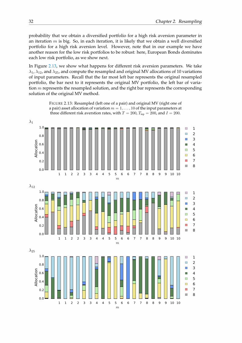
In Figure 2.13, we show what happens for different risk aversion parameters. We takeλ1, λ12, and λ25, and compute the resampled and original MV allocations of 10 variationsof input parameters. Recall that the far most left bar represents the original resampledportfolio, the bar next to it represents the original MV portfolio, the left bar of varia-tion m represents the resampled solution, and the right bar represents the correspondingsolution of the original MV method.
FIGURE 2.13: Resampled (left one of a pair) and original MV (right one ofa pair) asset allocation of variationm = 1, . . . , 10 of the input parameters atthree different risk averstion rates, with T = 200, Tinp = 200, and I = 200.
λ1
1 1 2 2 3 3 4 4 5 5 6 6 7 7 8 8 9 9 10 10m
0.0
0.2
0.4
0.6
0.8
1.0
Allo
cati
on
1
2
3
4
5
6
7
8
λ12
1 1 2 2 3 3 4 4 5 5 6 6 7 7 8 8 9 9 10 10m
0.0
0.2
0.4
0.6
0.8
1.0
Allo
cati
on
1
2
3
4
5
6
7
8
λ25
1 1 2 2 3 3 4 4 5 5 6 6 7 7 8 8 9 9 10 10m
0.0
0.2
0.4
0.6
0.8
1.0
Allo
cati
on
1
2
3
4
5
6
7
8
2.2. Example 33
We see that in our case, European Bonds dominates each low risk portfolio. Apparently,European Bonds has such strong characteristics, that the probability that in a variation amore diversified portfolio can attain the same level of return but a lower risk, is tiny; inthe 10 variations above, it does not occur. So, the initial strong characteristics of EuropeanBonds and the lack of asset classes with comparable characteristics are the reason for therobustness in our case. We see that for λ12, the portfolios are diversified; again with theresampled portfolios more diversified than the corresponding MV portfolios. Recall fromFigure 2.12, that the resampling method is more robust than the original MV method forλ12. So, here we see that the more diversified portfolios of the resampling method arealso more robust than the less diversified portfolios of the original MV method. Further-more, we see that for λ25, almost all the MV solutions of the variations put all weightin one asset class. Which asset class this is, varies per variation m. The correspondingresampled portfolios are a bit more diversified, but still extreme in their allocations. Wesee again, when we combine the results of Figure 2.12 with the results of Figure 2.13, thatthe more diversified portfolios of the resampling method are also more robust than theless diversified portfolios of the original MV method.
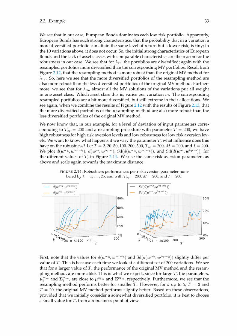
We now know that, in our example, for a level of deviation of input parameters corre-sponding to Tinp = 200 and a resampling procedure with parameter T = 200, we havehigh robustness for high risk aversion levels and low robustness for low risk aversion lev-els. We want to know what happens if we vary the parameter T ; what influence does thishave on the robustness? Let T = 2, 20, 50, 100, 200, 500, Tinp = 200, M = 200, and I = 200.We plot d(worig,winp orig), d(wres,winp res), Sd(d(worig,winp orig)), and Sd(d(wres,winp res)), forthe different values of T , in Figure 2.14. We use the same risk aversion parameters asabove and scale again towards the maximum distance.
FIGURE 2.14: Robustness performances per risk aversion parameter num-bered by k = 1, . . . , 25, and with Tinp = 200, M = 200, and I = 200.
k
0 510152025T
0 50100 200 5000%
20%
40%
60%
80%
d(worig ,winp orig )
d(wres ,winp res )
k
0 510152025T
0 50100 200 5000%
10%
20%
30%
Sd(d(worig ,winp orig ))
Sd(d(wres ,winp res ))
First, note that the values for d(worig,winp orig) and Sd(d(worig,winp orig)) slightly differ pervalue of T . This is because each time we look at a different set of 200 variations. We seethat for a larger value of T , the performance of the original MV method and the resam-pling method, are more alike. This is what we expect, since for large T , the parameters,µ
inpmi and Σ
inpmi , are close to µinpm and Σinpm , respectively. Furthermore, we see that the
resampling method performs better for smaller T . However, for k up to 5, T = 2 andT = 20, the original MV method performs slightly better. Based on these observations,provided that we initially consider a somewhat diversified portfolio, it is best to choosea small value for T , from a robustness point of view.
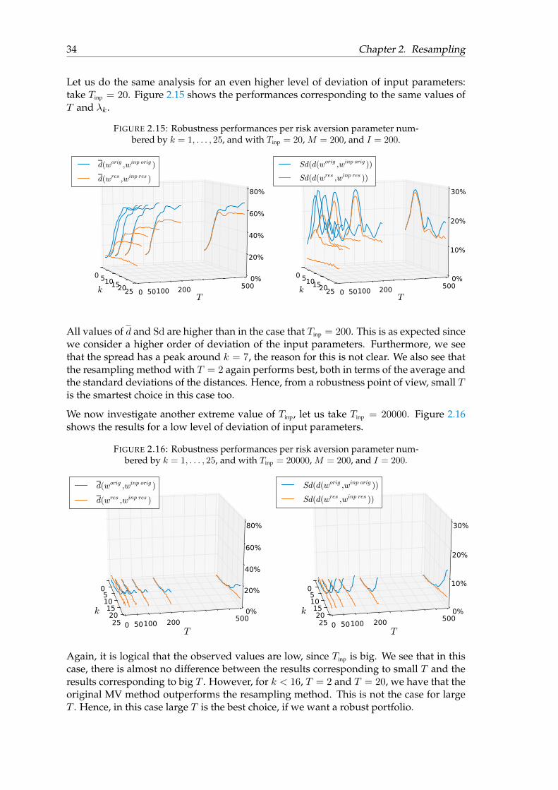
34 Chapter 2. Resampling
Let us do the same analysis for an even higher level of deviation of input parameters:take Tinp = 20. Figure 2.15 shows the performances corresponding to the same values ofT and λk.
FIGURE 2.15: Robustness performances per risk aversion parameter num-bered by k = 1, . . . , 25, and with Tinp = 20, M = 200, and I = 200.
k
0 510152025T
0 50100 200 5000%
20%
40%
60%
80%
d(worig ,winp orig )
d(wres ,winp res )
k
0 510152025T
0 50100 200 5000%
10%
20%
30%
Sd(d(worig ,winp orig ))
Sd(d(wres ,winp res ))
All values of d and Sd are higher than in the case that Tinp = 200. This is as expected sincewe consider a higher order of deviation of the input parameters. Furthermore, we seethat the spread has a peak around k = 7, the reason for this is not clear. We also see thatthe resampling method with T = 2 again performs best, both in terms of the average andthe standard deviations of the distances. Hence, from a robustness point of view, small Tis the smartest choice in this case too.
We now investigate another extreme value of Tinp, let us take Tinp = 20000. Figure 2.16shows the results for a low level of deviation of input parameters.
FIGURE 2.16: Robustness performances per risk aversion parameter num-bered by k = 1, . . . , 25, and with Tinp = 20000, M = 200, and I = 200.
k
0510152025
T0 50100 200 500
0%
20%
40%
60%
80%
d(worig ,winp orig )
d(wres ,winp res )
k
0510152025
T0 50100 200 500
0%
10%
20%
30%
Sd(d(worig ,winp orig ))
Sd(d(wres ,winp res ))
Again, it is logical that the observed values are low, since Tinp is big. We see that in thiscase, there is almost no difference between the results corresponding to small T and theresults corresponding to big T . However, for k < 16, T = 2 and T = 20, we have that theoriginal MV method outperforms the resampling method. This is not the case for largeT . Hence, in this case large T is the best choice, if we want a robust portfolio.
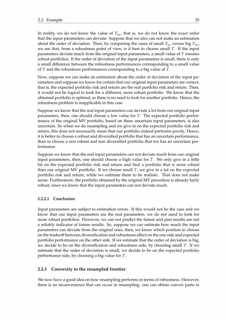
2.2. Example 35
In reality, we do not know the value of Tinp, that is, we do not know the exact orderthat the input parameters can deviate. Suppose that we also can not make an estimationabout the order of deviation. Then, by comparing the cases of small Tinp versus big Tinp,we see that, from a robustness point of view, is it best to choose small T . If the inputparameters deviate much from the original input parameters, a small value of T ensuresrobust portfolios. If the order of deviation of the input parameters is small, there is onlya small difference between the robustness performances corresponding to a small valueof T and the robustness performances corresponding to a big value of T .
Now, suppose we can make an estimation about the order of deviation of the input pa-rameters and suppose we know for certain that our original input parameters are correct,that is, the expected portfolio risk and return are the real portfolio risk and return. Then,it would not be logical to look for a different, more robust portfolio. We know that theobtained portfolio is optimal, so there is no need to look for another portfolio. Hence, therobustness problem is inapplicable in this case.
Suppose we know that the real input parameters can deviate a lot from our original inputparameters, then, one should choose a low value for T . The expected portfolio perfor-mance of the original MV portfolio, based on these uncertain input parameters, is alsouncertain. So when we do resampling and we give in on the expected portfolio risk andreturn, this does not necessarily mean that our portfolio indeed performs poorly. Hence,it is better to choose a robust and diversified portfolio that has an uncertain performance,than to choose a non robust and non diversified portfolio that too has an uncertain per-formance.
Suppose we know that the real input parameters can not deviate much from our originalinput parameters, then, one should choose a high value for T . We only give in a littlebit on the expected portfolio risk and return and find a portfolio that is more robustthan our original MV portfolio. If we choose small T , we give in a lot on the expectedportfolio risk and return, while we estimate them to be realistic. That does not makesense. Furthermore, the portfolio obtained by the original MV procedure is already fairlyrobust, since we know that the input parameters can not deviate much.
2.2.2.1 Conclusion
Input parameters are subject to estimation errors. If this would not be the case and weknow that our input parameters are the real parameters, we do not need to look formore robust portfolios. However, we can not predict the future and past results are nota reliably indicator of future results. So, suppose we can estimate how much the inputparameters can deviate from the original ones, then, we know which position to chooseon the tradeoff between diversification and robustness effect on the one side and expectedportfolio performance on the other side. If we estimate that the order of deviation is big,we decide to be on the diversification and robustness side, by choosing small T . If weestimate that the order of deviation is small, we decide to be on the expected portfolioperformance side, by choosing a big value for T .
2.2.3 Convexity in the resampled frontier
We now have a good idea on how resampling performs in terms of robustness. However,there is an inconvenience that can occur in resampling: one can obtain convex parts in
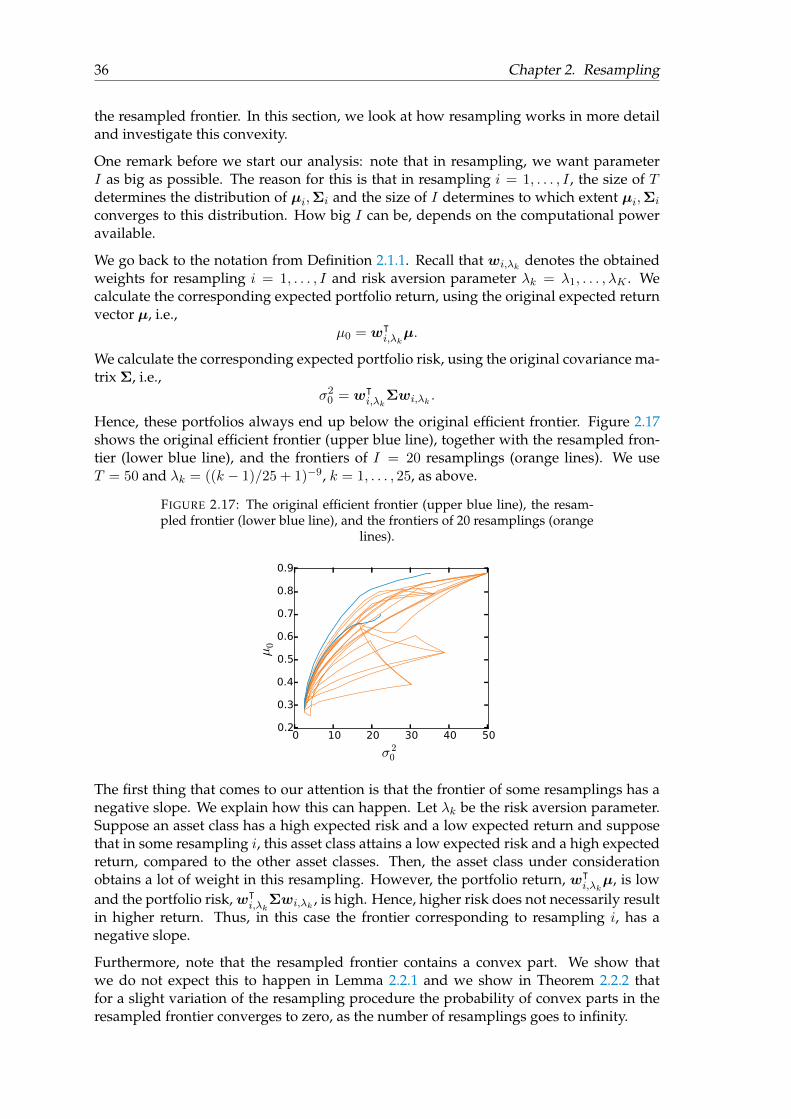
36 Chapter 2. Resampling
the resampled frontier. In this section, we look at how resampling works in more detailand investigate this convexity.
One remark before we start our analysis: note that in resampling, we want parameterI as big as possible. The reason for this is that in resampling i = 1, . . . , I , the size of Tdetermines the distribution of µi,Σi and the size of I determines to which extent µi,Σi
converges to this distribution. How big I can be, depends on the computational poweravailable.
We go back to the notation from Definition 2.1.1. Recall that wi,λk denotes the obtainedweights for resampling i = 1, . . . , I and risk aversion parameter λk = λ1, . . . , λK . Wecalculate the corresponding expected portfolio return, using the original expected returnvector µ, i.e.,
µ0 = wᵀi,λkµ.
We calculate the corresponding expected portfolio risk, using the original covariance ma-trix Σ, i.e.,
σ20 = wᵀi,λk
Σwi,λk .
Hence, these portfolios always end up below the original efficient frontier. Figure 2.17shows the original efficient frontier (upper blue line), together with the resampled fron-tier (lower blue line), and the frontiers of I = 20 resamplings (orange lines). We useT = 50 and λk = ((k − 1)/25 + 1)−9, k = 1, . . . , 25, as above.
FIGURE 2.17: The original efficient frontier (upper blue line), the resam-pled frontier (lower blue line), and the frontiers of 20 resamplings (orange
lines).
0 10 20 30 40 50
σ 20
0.2
0.3
0.4
0.5
0.6
0.7
0.8
0.9
µ0
The first thing that comes to our attention is that the frontier of some resamplings has anegative slope. We explain how this can happen. Let λk be the risk aversion parameter.Suppose an asset class has a high expected risk and a low expected return and supposethat in some resampling i, this asset class attains a low expected risk and a high expectedreturn, compared to the other asset classes. Then, the asset class under considerationobtains a lot of weight in this resampling. However, the portfolio return, wᵀ
i,λkµ, is low
and the portfolio risk,wᵀi,λk
Σwi,λk , is high. Hence, higher risk does not necessarily resultin higher return. Thus, in this case the frontier corresponding to resampling i, has anegative slope.
Furthermore, note that the resampled frontier contains a convex part. We show thatwe do not expect this to happen in Lemma 2.2.1 and we show in Theorem 2.2.2 thatfor a slight variation of the resampling procedure the probability of convex parts in theresampled frontier converges to zero, as the number of resamplings goes to infinity.
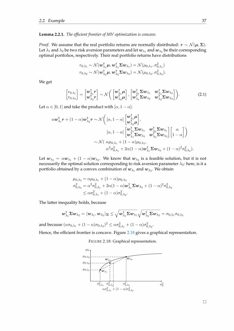
2.2. Example 37
Lemma 2.2.1. The efficient frontier of MV optimization is concave.
Proof. We assume that the real portfolio returns are normally distributed: r ∼ N (µ,Σ).Let λ1 and λ2 be two risk aversion parameters and letwλ1 andwλ2 be their correspondingoptimal portfolios, respectively. Their real portfolio returns have distributions
r0,λ1 ∼ N (wᵀλ1µ,wᵀ
λ1Σwλ1) = N (µ0,λ1 , σ
20,λ1)
r0,λ2 ∼ N (wᵀλ2µ,wᵀ
λ2Σwλ2) = N (µ0,λ2 , σ
20,λ2).
We get [r0,λ1r0,λ2
]=
[wᵀλ1r
wᵀλ2r
]∼ N
([wᵀλ1µ
wᵀλ2µ
],
[wᵀλ1
Σwλ1 wᵀλ1
Σwλ2
wᵀλ1
Σwλ2 wᵀλ2
Σwλ2
]). (2.1)
Let α ∈ [0, 1] and take the product with [α, 1− α]:
αwᵀλ1r + (1− α)wᵀ
λ2r ∼ N
([α, 1− α]
[wᵀλ1µ
wᵀλ2µ
],
[α, 1− α]
[wᵀλ1
Σwλ1 wᵀλ2
Σwλ1
wᵀλ1
Σwλ2 wᵀλ2
Σwλ2
][α
1− α
])∼ N ( αµ0,λ1 + (1− α)µ0,λ2 ,
α2σ20,λ1 + 2α(1− α)wᵀλ1
Σwλ2 + (1− α)2σ20,λ2).
Let wλ3 = αwλ1 + (1 − α)wλ2 . We know that wλ3 is a feasible solution, but it is notnecessarily the optimal solution corresponding to risk aversion parameter λ3: here, is it aportfolio obtained by a convex combination of wλ1 and wλ2 . We obtain
µ0,λ3 = αµ0,λ1 + (1− α)µ0,λ2
σ20,λ3 = α2σ20,λ1 + 2α(1− α)wᵀλ1
Σwλ2 + (1− α)2σ20,λ2
≤ ασ20,λ1 + (1− α)σ20,λ2 .
The latter inequality holds, because
wᵀλ1
Σwλ2 = 〈wλ1 ,wλ2〉Σ ≤√wᵀλ1
Σwλ1
√wᵀλ2
Σwλ2 = σ0,λ1σ0,λ2
and because (ασ0,λ1 + (1− α)σ0,λ2)2 ≤ ασ20,λ1 + (1− α)σ20,λ2 .
Hence, the efficient frontier is concave. Figure 2.18 gives a graphical representation.
FIGURE 2.18: Graphical representation.
σ20
µ0
wλ2
wλ1
wλ3
µ0,λ1
µ0,λ2
µ0,λ3
σ20,λ1 σ20,λ2σ20,λ3ασ20,λ1 + (1− α)σ20,λ2
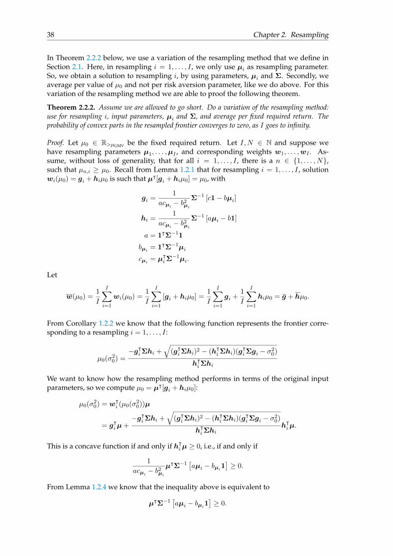
38 Chapter 2. Resampling
In Theorem 2.2.2 below, we use a variation of the resampling method that we define inSection 2.1. Here, in resampling i = 1, . . . , I , we only use µi as resampling parameter.So, we obtain a solution to resampling i, by using parameters, µi and Σ. Secondly, weaverage per value of µ0 and not per risk aversion parameter, like we do above. For thisvariation of the resampling method we are able to proof the following theorem.
Theorem 2.2.2. Assume we are allowed to go short. Do a variation of the resampling method:use for resampling i, input parameters, µi and Σ, and average per fixed required return. Theprobability of convex parts in the resampled frontier converges to zero, as I goes to infinity.
Proof. Let µ0 ∈ R>µGMV be the fixed required return. Let I,N ∈ N and suppose wehave resampling parameters µ1, . . . ,µI , and corresponding weights w1, . . . ,wI . As-sume, without loss of generality, that for all i = 1, . . . , I , there is a n ∈ {1, . . . , N},such that µn,i ≥ µ0. Recall from Lemma 1.2.1 that for resampling i = 1, . . . , I , solutionwi(µ0) = gi + hiµ0 is such that µᵀ[gi + hiµ0] = µ0, with
gi =1
acµi− b2µi
Σ−1 [c1− bµi]
hi =1
acµi− b2µi
Σ−1 [aµi − b1]
a = 1ᵀΣ−11
bµi= 1ᵀΣ−1µi
cµi= µᵀ
iΣ−1µi.
Let
w(µ0) =1
I
I∑i=1
wi(µ0) =1
I
I∑i=1
[gi + hiµ0] =1
I
I∑i=1
gi +1
I
I∑i=1
hiµ0 = g + hµ0.
From Corollary 1.2.2 we know that the following function represents the frontier corre-sponding to a resampling i = 1, . . . , I :
µ0(σ20) =
−gᵀiΣhi +√
(gᵀiΣhi)2 − (hᵀ
iΣhi)(gᵀiΣgi − σ20)
hᵀiΣhi
We want to know how the resampling method performs in terms of the original inputparameters, so we compute µ0 = µᵀ[gi + hiµ0]:
µ0(σ20) = wᵀ
i (µ0(σ20))µ
= gᵀiµ+−gᵀiΣhi +
√(gᵀiΣhi)
2 − (hᵀiΣhi)(g
ᵀiΣgi − σ20)
hᵀiΣhi
hᵀiµ.
This is a concave function if and only if hᵀiµ ≥ 0, i.e., if and only if
1
acµi− b2µi
µᵀΣ−1[aµi − bµi
1]≥ 0.
From Lemma 1.2.4 we know that the inequality above is equivalent to
µᵀΣ−1[aµi − bµi
1]≥ 0.
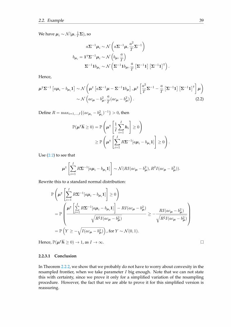
2.2. Example 39
We have µi ∼ N (µ, 1T Σ), so
aΣ−1µi ∼ N(aΣ−1µ,
a2
TΣ−1
)bµi
= 1ᵀΣ−1µi ∼ N(bµ,
a
T
)Σ−11bµi
∼ N(Σ−11bµ,
a
T
[Σ−11
] [Σ−11
]ᵀ).
Hence,
µᵀΣ−1[aµi − bµi
1]∼ N
(µᵀ [aΣ−1µ−Σ−11bµ
],µᵀ
[a2
TΣ−1 − a
T
[Σ−11
] [Σ−11
]ᵀ]µ
)∼ N
(acµ − b2µ,
a
T(acµ − b2µ)
). (2.2)
Define R = maxi=1,...,I{(acµi− b2µi
)−1} > 0, then
P(µᵀh ≥ 0) = P
(µᵀ
[1
I
I∑i=1
hi
]≥ 0
)
≥ P
(µᵀ
[I∑i=1
RΣ−1[aµi − bµi1]
]≥ 0
).
Use (2.2) to see that
µᵀ
[I∑i=1
RΣ−1[aµi − bµi1]
]∼ N (RI(acµ − b2µ), R2I(acµ − b2µ)).
Rewrite this to a standard normal distribution:
P
(µᵀ
[I∑i=1
RΣ−1[aµi − bµi1]
]≥ 0
)
= P
µᵀ
[I∑i=1
RΣ−1[aµi − bµi1]
]−RI(acµ − b2µ)√
R2I(acµ − b2µ)≥ −
RI(acµ − b2µ)√R2I(acµ − b2µ)
= P
(Y ≥ −
√I(acµ − b2µ)
), for Y ∼ N (0, 1).
Hence, P(µᵀh ≥ 0)→ 1, as I →∞.
2.2.3.1 Conclusion
In Theorem 2.2.2, we show that we probably do not have to worry about convexity in theresampled frontier, when we take parameter I big enough. Note that we can not statethis with certainty, since we prove it only for a simplified variation of the resamplingprocedure. However, the fact that we are able to prove it for this simplified version isreassuring.

41
Chapter 3
Shrinkage
In the previous chapter, we discuss the resampling method; a procedure that makes theMV optimization method more robust, given the estimated input parameters. In thischapter, we look at a procedure that tries to make the parameter estimation more robust:shrinkage. In MV optimization, we use the sample means and the sample covariancematrix. In the shrinkage method, we still use the sample means, but another covariancematrix: a shrunken covariance matrix. We investigate what effect a shrunken covariancematrix has on the robustness of the MV optimization method. We use the shrinkagemethod introduced by Ledoit and Wolf [6]. They look at a variation of the shrinkagemethod, which can be used when there many stocks, but only a few historical data pointsavailable. They explain
“(...) when there are many stocks under consideration, especially comparedto the number of historical return observations available (as is the usual case),the sample covariance matrix is estimated with a lot of error. This means themost extreme coefficients in such an estimated matrix tend to take on extremevalues, not because they are correct but because they are subject to an ex-treme amount of error. Invariably the mean-variance optimization softwarewill latch onto the extremes, and place its biggest bets on the coefficients thatare the most unreliable.” [6].
Ortec Finance uses a Monte Carlo method to generate economic scenarios, in which allkind of future states of global economies and capital markets are simulated. The numberof scenarios that is generated is large. Hence, in our case we have many data points,compared to the number of stocks under consideration. We investigate whether or notthe shrinkage method is still useful.
3.1 Formulation
We define the shrinkage procedure for the covariance matrix. Let Γ ∈ RN × RN denotethe shrinkage target; sometimes we abbreviate it to target. Let δ ∈ [0, 1] be the shrinkageparameter.
Definition 3.1.1. The shrinkage procedure is as follows. We have the sample covariancematrix Σ and we have a target Γ. The amount of shrinkage towards the target, is deter-mined by the value of δ. The covariance matrix we obtain, by shrinking Σ towards Γ, isδΣ + (1− δ)Γ.
We call δΣ + (1− δ)Γ the shrunken covariance matrix.
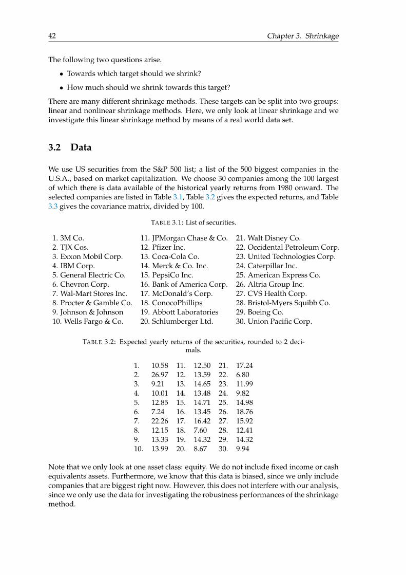
42 Chapter 3. Shrinkage
The following two questions arise.
• Towards which target should we shrink?
• How much should we shrink towards this target?
There are many different shrinkage methods. These targets can be split into two groups:linear and nonlinear shrinkage methods. Here, we only look at linear shrinkage and weinvestigate this linear shrinkage method by means of a real world data set.
3.2 Data
We use US securities from the S&P 500 list; a list of the 500 biggest companies in theU.S.A., based on market capitalization. We choose 30 companies among the 100 largestof which there is data available of the historical yearly returns from 1980 onward. Theselected companies are listed in Table 3.1, Table 3.2 gives the expected returns, and Table3.3 gives the covariance matrix, divided by 100.
TABLE 3.1: List of securities.
1. 3M Co. 11. JPMorgan Chase & Co. 21. Walt Disney Co.2. TJX Cos. 12. Pfizer Inc. 22. Occidental Petroleum Corp.3. Exxon Mobil Corp. 13. Coca-Cola Co. 23. United Technologies Corp.4. IBM Corp. 14. Merck & Co. Inc. 24. Caterpillar Inc.5. General Electric Co. 15. PepsiCo Inc. 25. American Express Co.6. Chevron Corp. 16. Bank of America Corp. 26. Altria Group Inc.7. Wal-Mart Stores Inc. 17. McDonald’s Corp. 27. CVS Health Corp.8. Procter & Gamble Co. 18. ConocoPhillips 28. Bristol-Myers Squibb Co.9. Johnson & Johnson 19. Abbott Laboratories 29. Boeing Co.10. Wells Fargo & Co. 20. Schlumberger Ltd. 30. Union Pacific Corp.
TABLE 3.2: Expected yearly returns of the securities, rounded to 2 deci-mals.
1. 10.58 11. 12.50 21. 17.242. 26.97 12. 13.59 22. 6.803. 9.21 13. 14.65 23. 11.994. 10.01 14. 13.48 24. 9.825. 12.85 15. 14.71 25. 14.986. 7.24 16. 13.45 26. 18.767. 22.26 17. 16.42 27. 15.928. 12.15 18. 7.60 28. 12.419. 13.33 19. 14.32 29. 14.3210. 13.99 20. 8.67 30. 9.94
Note that we only look at one asset class: equity. We do not include fixed income or cashequivalents assets. Furthermore, we know that this data is biased, since we only includecompanies that are biggest right now. However, this does not interfere with our analysis,since we only use the data for investigating the robustness performances of the shrinkagemethod.
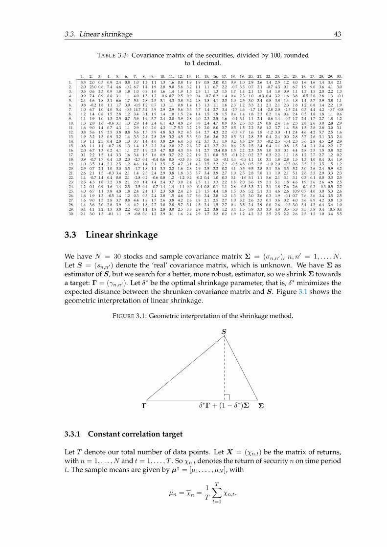
3.3. Linear shrinkage 43
TABLE 3.3: Covariance matrix of the securities, divided by 100, roundedto 1 decimal.
1. 2. 3. 4. 5. 6. 7. 8. 9. 10. 11. 12. 13. 14. 15. 16. 17. 18. 19. 20. 21. 22. 23. 24. 25. 26. 27. 28. 29. 30.1. 3.3 2.0 0.5 0.9 2.4 0.8 1.0 1.2 1.1 1.3 1.6 0.8 1.9 1.9 0.8 2.0 0.1 0.9 1.0 2.9 2.6 1.4 2.5 1.2 4.0 1.6 1.6 1.4 3.4 2.12. 2.0 23.0 0.6 7.4 4.6 −0.2 6.7 1.4 1.9 2.8 9.0 5.6 3.2 1.1 1.1 6.7 2.2 −0.7 3.5 0.7 2.1 −0.7 4.3 0.1 6.7 1.9 9.0 3.6 4.1 3.03. 0.5 0.6 2.3 0.9 1.8 1.8 1.0 0.8 1.0 1.6 1.4 1.9 1.3 2.5 1.1 1.3 1.5 1.7 1.4 2.1 1.5 1.4 1.8 0.9 1.1 1.3 1.5 2.0 2.2 1.34. 0.9 7.4 0.9 8.8 3.1 1.1 4.0 1.5 1.3 −0.6 0.7 2.5 0.9 0.4 −0.7 0.2 1.4 0.4 2.3 1.0 −0.3 0.4 3.2 1.6 3.8 −0.5 2.8 2.8 1.3 −0.15. 2.4 4.6 1.8 3.1 6.6 1.7 5.4 2.8 2.5 3.1 4.3 3.8 3.2 2.8 1.8 4.1 3.3 1.0 2.5 3.0 3.4 0.8 3.8 1.4 4.8 1.4 3.7 3.9 3.8 1.16. 0.8 −0.2 1.8 1.1 1.7 3.0 −0.5 1.2 0.7 1.3 1.1 0.8 1.4 1.3 1.3 1.1 1.6 2.3 1.2 3.3 2.1 2.1 2.1 2.3 1.8 1.2 0.8 1.4 2.2 1.97. 1.0 6.7 1.0 4.0 5.4 −0.5 14.7 3.4 3.9 2.9 2.9 5.6 3.3 3.7 1.4 2.7 3.4 −2.7 4.6 −1.7 1.4 −2.8 2.0 −2.5 2.4 0.3 4.4 4.2 −0.7 −0.88. 1.2 1.4 0.8 1.5 2.8 1.2 3.4 3.1 1.9 1.4 1.0 1.5 2.4 1.4 1.5 1.9 1.5 0.4 1.4 1.8 2.3 0.2 1.4 0.4 2.4 0.5 1.8 1.8 1.1 0.69. 1.1 1.9 1.0 1.3 2.5 0.7 3.9 1.9 3.7 2.4 2.0 3.9 2.8 4.0 2.3 2.5 1.6 −0.4 3.1 1.1 2.4 −0.6 1.4 −0.7 1.7 2.4 1.7 2.7 1.8 1.210. 1.3 2.8 1.6 −0.6 3.1 1.3 2.9 1.4 2.4 6.1 4.3 4.8 2.9 3.8 2.4 4.7 0.9 0.6 2.5 3.3 2.9 0.8 2.4 1.4 2.3 2.8 2.6 3.0 2.8 2.911. 1.6 9.0 1.4 0.7 4.3 1.1 2.9 1.0 2.0 4.3 11.7 5.3 3.2 2.9 2.0 8.0 3.7 0.5 1.5 2.2 3.8 1.2 3.7 1.4 5.8 1.5 3.8 2.8 3.0 3.112. 0.8 5.6 1.9 2.5 3.8 0.8 5.6 1.5 3.9 4.8 5.3 9.2 4.5 6.4 2.7 4.3 2.2 −0.3 4.7 1.6 1.8 −1.2 3.0 −1.1 2.4 4.6 4.2 5.7 2.5 1.613. 1.9 3.2 1.3 0.9 3.2 1.4 3.3 2.4 2.8 2.9 3.2 4.5 5.3 5.0 2.6 3.6 2.2 0.5 3.1 2.8 3.5 0.4 2.4 0.0 2.8 3.7 2.6 3.1 3.3 2.414. 1.9 1.1 2.5 0.4 2.8 1.3 3.7 1.4 4.0 3.8 2.9 6.4 5.0 9.2 3.7 3.1 1.9 0.2 4.3 2.9 3.7 −0.2 2.5 −0.4 2.3 5.6 2.8 4.5 2.9 2.915. 0.8 1.1 1.1 −0.7 1.8 1.3 1.4 1.5 2.3 2.4 2.0 2.7 2.6 3.7 4.3 2.7 2.1 0.6 2.5 2.5 3.4 0.4 1.1 0.8 1.5 3.4 2.1 2.4 2.2 1.716. 2.0 6.7 1.3 0.2 4.1 1.1 2.7 1.9 2.5 4.7 8.0 4.3 3.6 3.1 2.7 13.4 0.8 1.5 2.2 2.3 3.9 1.0 3.3 0.1 4.4 2.8 2.5 1.5 3.8 3.217. 0.1 2.2 1.5 1.4 3.3 1.6 3.4 1.5 1.6 0.9 3.7 2.2 2.2 1.9 2.1 0.8 5.5 −0.1 2.2 0.2 2.7 0.3 2.2 1.1 1.8 1.2 2.7 2.7 1.2 0.218. 0.9 −0.7 1.7 0.4 1.0 2.3 −2.7 0.4 −0.4 0.6 0.5 −0.3 0.5 0.2 0.6 1.5 −0.1 4.4 −0.5 4.1 1.0 3.1 1.8 2.8 1.5 1.3 1.0 0.4 3.4 1.919. 1.0 3.5 1.4 2.3 2.5 1.2 4.6 1.4 3.1 2.5 1.5 4.7 3.1 4.3 2.5 2.2 2.2 −0.5 4.8 0.5 2.5 −1.0 2.0 −0.5 0.6 3.5 3.2 3.5 1.5 1.220. 2.9 0.7 2.1 1.0 3.0 3.3 −1.7 1.8 1.1 3.3 2.2 1.6 2.8 2.9 2.5 2.3 0.2 4.1 0.5 9.5 2.8 5.1 3.6 3.3 5.2 3.0 2.6 2.4 5.9 4.221. 2.6 2.1 1.5 −0.3 3.4 2.1 1.4 2.3 2.4 2.9 3.8 1.8 3.5 3.7 3.4 3.9 2.7 1.0 2.5 2.8 7.8 1.1 1.9 2.1 5.1 2.6 3.3 2.9 3.3 2.322. 1.4 −0.7 1.4 0.4 0.8 2.1 −2.8 0.2 −0.6 0.8 1.2 −1.2 0.4 −0.2 0.4 1.0 0.3 3.1 −1.0 5.1 1.1 5.6 2.1 3.1 3.1 0.3 0.1 0.0 3.3 2.523. 2.5 4.3 1.8 3.2 3.8 2.1 2.0 1.4 1.4 2.4 3.7 3.0 2.4 2.5 1.1 3.3 2.2 1.8 2.0 3.6 1.9 2.1 5.1 1.8 4.6 1.9 3.6 2.6 4.8 2.524. 1.2 0.1 0.9 1.6 1.4 2.3 −2.5 0.4 −0.7 1.4 1.4 −1.1 0.0 −0.4 0.8 0.1 1.1 2.8 −0.5 3.3 2.1 3.1 1.8 7.6 2.6 −0.1 0.2 −0.3 0.5 2.225. 4.0 6.7 1.1 3.8 4.8 1.8 2.4 2.4 1.7 2.3 5.8 2.4 2.8 2.3 1.5 4.4 1.8 1.5 0.6 5.2 5.1 3.1 4.6 2.6 10.9 0.7 4.0 3.0 5.3 2.626. 1.6 1.9 1.3 −0.5 1.4 1.2 0.3 0.5 2.4 2.8 1.5 4.6 3.7 5.6 3.4 2.8 1.2 1.3 3.5 3.0 2.6 0.3 1.9 −0.1 0.7 7.6 3.6 3.4 3.5 2.527. 1.6 9.0 1.5 2.8 3.7 0.8 4.4 1.8 1.7 2.6 3.8 4.2 2.6 2.8 2.1 2.5 2.7 1.0 3.2 2.6 3.3 0.1 3.6 0.2 4.0 3.6 8.9 4.2 3.8 1.328. 1.4 3.6 2.0 2.8 3.9 1.4 4.2 1.8 2.7 3.0 2.8 5.7 3.1 4.5 2.4 1.5 2.7 0.4 3.5 2.4 2.9 0.0 2.6 −0.3 3.0 3.4 4.2 6.4 3.4 1.029. 3.4 4.1 2.2 1.3 3.8 2.2 −0.7 1.1 1.8 2.8 3.0 2.5 3.3 2.9 2.2 3.8 1.2 3.4 1.5 5.9 3.3 3.3 4.8 0.5 5.3 3.5 3.8 3.4 10.5 3.430. 2.1 3.0 1.3 −0.1 1.1 1.9 −0.8 0.6 1.2 2.9 3.1 1.6 2.4 2.9 1.7 3.2 0.2 1.9 1.2 4.2 2.3 2.5 2.5 2.2 2.6 2.5 1.3 1.0 3.4 5.5
3.3 Linear shrinkage
We have N = 30 stocks and sample covariance matrix Σ = (σn,n′), n, n′ = 1, . . . , N .Let S = (sn,n′) denote the ‘real’ covariance matrix, which is unknown. We have Σ asestimator of S, but we search for a better, more robust, estimator, so we shrink Σ towardsa target: Γ = (γn,n′). Let δ∗ be the optimal shrinkage parameter, that is, δ∗ minimizes theexpected distance between the shrunken covariance matrix and S. Figure 3.1 shows thegeometric interpretation of linear shrinkage.
FIGURE 3.1: Geometric interpretation of the shrinkage method.
S
Γ Σδ∗Γ + (1− δ∗)Σ
3.3.1 Constant correlation target
Let T denote our total number of data points. Let X = (χn,t) be the matrix of returns,with n = 1, . . . , N and t = 1, . . . , T . So χn,t denotes the return of security n on time periodt. The sample means are given by µᵀ = [µ1, . . . , µN ], with
µn = χn =1
T
T∑t=1
χn,t.
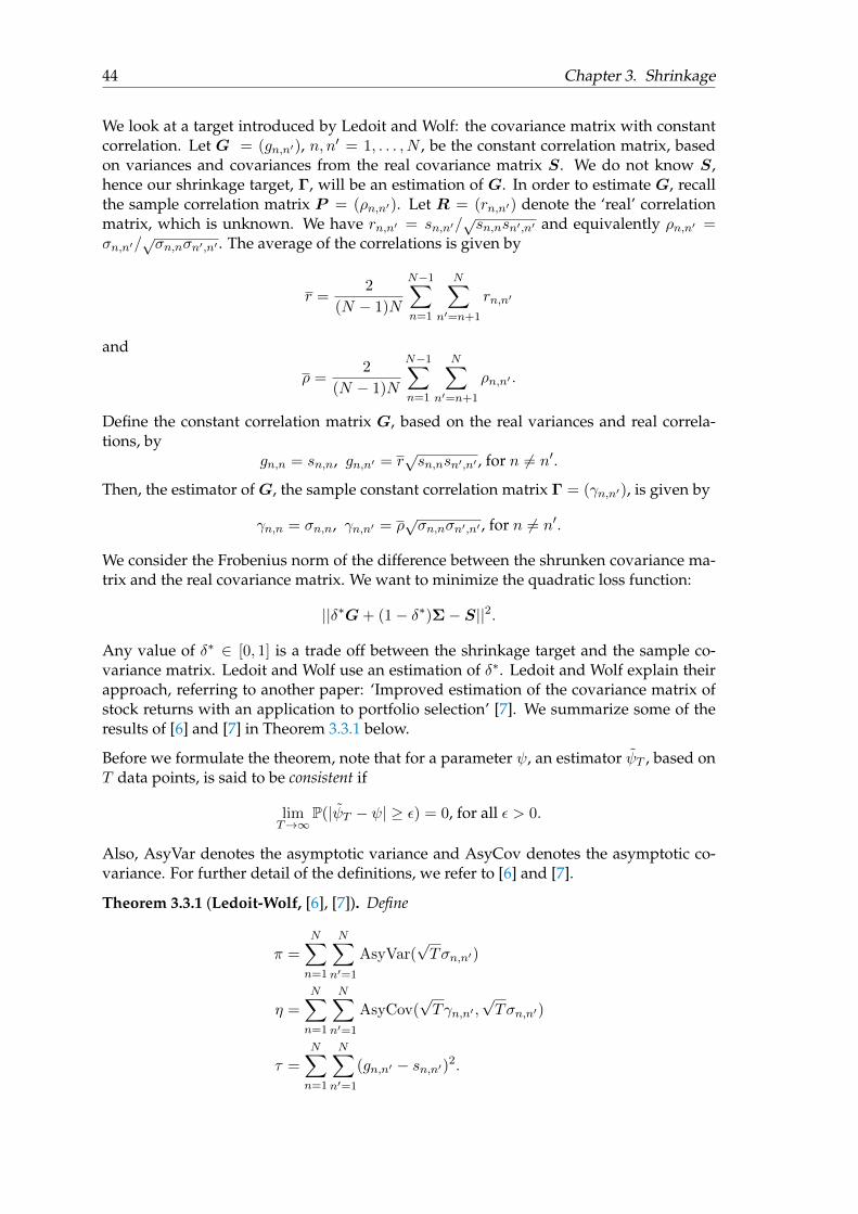
44 Chapter 3. Shrinkage
We look at a target introduced by Ledoit and Wolf: the covariance matrix with constantcorrelation. Let G = (gn,n′), n, n′ = 1, . . . , N , be the constant correlation matrix, basedon variances and covariances from the real covariance matrix S. We do not know S,hence our shrinkage target, Γ, will be an estimation of G. In order to estimate G, recallthe sample correlation matrix P = (ρn,n′). Let R = (rn,n′) denote the ‘real’ correlationmatrix, which is unknown. We have rn,n′ = sn,n′/
√sn,nsn′,n′ and equivalently ρn,n′ =
σn,n′/√σn,nσn′,n′ . The average of the correlations is given by
r =2
(N − 1)N
N−1∑n=1
N∑n′=n+1
rn,n′
and
ρ =2
(N − 1)N
N−1∑n=1
N∑n′=n+1
ρn,n′ .
Define the constant correlation matrix G, based on the real variances and real correla-tions, by
gn,n = sn,n, gn,n′ = r√sn,nsn′,n′ , for n 6= n′.
Then, the estimator ofG, the sample constant correlation matrix Γ = (γn,n′), is given by
γn,n = σn,n, γn,n′ = ρ√σn,nσn′,n′ , for n 6= n′.
We consider the Frobenius norm of the difference between the shrunken covariance ma-trix and the real covariance matrix. We want to minimize the quadratic loss function:
||δ∗G+ (1− δ∗)Σ− S||2.
Any value of δ∗ ∈ [0, 1] is a trade off between the shrinkage target and the sample co-variance matrix. Ledoit and Wolf use an estimation of δ∗. Ledoit and Wolf explain theirapproach, referring to another paper: ‘Improved estimation of the covariance matrix ofstock returns with an application to portfolio selection’ [7]. We summarize some of theresults of [6] and [7] in Theorem 3.3.1 below.
Before we formulate the theorem, note that for a parameter ψ, an estimator ψ̃T , based onT data points, is said to be consistent if
limT→∞
P(|ψ̃T − ψ| ≥ ε) = 0, for all ε > 0.
Also, AsyVar denotes the asymptotic variance and AsyCov denotes the asymptotic co-variance. For further detail of the definitions, we refer to [6] and [7].
Theorem 3.3.1 (Ledoit-Wolf, [6], [7]). Define
π =
N∑n=1
N∑n′=1
AsyVar(√Tσn,n′)
η =N∑n=1
N∑n′=1
AsyCov(√Tγn,n′ ,
√Tσn,n′)
τ =N∑n=1
N∑n′=1
(gn,n′ − sn,n′)2.
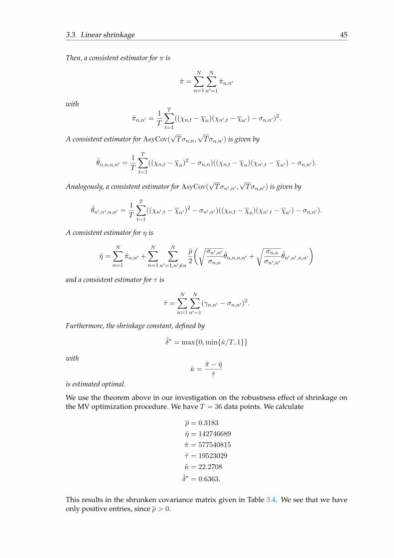
3.3. Linear shrinkage 45
Then, a consistent estimator for π is
π̂ =N∑n=1
N∑n′=1
π̂n,n′
with
π̂n,n′ =1
T
T∑t=1
((χn,t − χn)(χn′,t − χn′)− σn,n′)2.
A consistent estimator for AsyCov(√Tσn,n,
√Tσn,n′) is given by
θ̂n,n,n,n′ =1
T
T∑t=1
((χn,t − χn)2 − σn,n)((χn,t − χn)(χn′,t − χn′)− σn,n′).
Analogously, a consistent estimator for AsyCov(√Tσn′,n′ ,
√Tσn,n′) is given by
θ̂n′,n′,n,n′ =1
T
T∑t=1
((χn′,t − χn′)2 − σn′,n′)((χn,t − χn)(χn′,t − χn′)− σn,n′).
A consistent estimator for η is
η̂ =
N∑n=1
π̂n,n′ +
N∑n=1
N∑n′=1,n′ 6=n
ρ
2
(√σn′,n′
σn,nθ̂n,n,n,n′ +
√σn,nσn′,n′
θ̂n′,n′,n,n′
)
and a consistent estimator for τ is
τ̂ =N∑n=1
N∑n′=1
(γn,n′ − σn,n′)2.
Furthermore, the shrinkage constant, defined by
δ̂∗ = max{0,min{κ̂/T, 1}}
withκ̂ =
π̂ − η̂τ̂
is estimated optimal.
We use the theorem above in our investigation on the robustness effect of shrinkage onthe MV optimization procedure. We have T = 36 data points. We calculate
ρ = 0.3183
η̂ = 142746689
π̂ = 577540815
τ̂ = 19523029
κ̂ = 22.2708
δ̂∗ = 0.6363.
This results in the shrunken covariance matrix given in Table 3.4. We see that we haveonly positive entries, since ρ > 0.
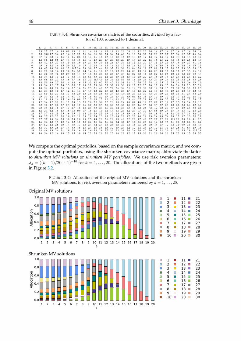
46 Chapter 3. Shrinkage
TABLE 3.4: Shrunken covariance matrix of the securities, divided by a fac-tor of 100, rounded to 1 decimal.
1. 2. 3. 4. 5. 6. 7. 8. 9. 10. 11. 12. 13. 14. 15. 16. 17. 18. 19. 20. 21. 22. 23. 24. 25. 26. 27. 28. 29. 30.1. 3.3 2.5 0.7 1.4 1.8 0.9 1.8 1.1 1.1 1.4 1.8 1.4 1.5 1.8 1.1 2.1 0.9 1.1 1.2 2.2 2.0 1.4 1.7 1.4 2.7 1.6 1.7 1.4 2.4 1.62. 2.5 23.0 1.7 5.6 4.2 1.6 6.2 2.2 2.6 3.4 6.6 5.0 3.4 3.4 2.4 6.0 3.1 1.8 3.4 3.2 3.5 2.1 3.7 2.7 5.7 3.4 6.2 3.7 4.6 3.43. 0.7 1.7 2.3 1.2 1.5 1.2 1.6 0.8 0.9 1.4 1.6 1.6 1.2 1.8 1.0 1.6 1.2 1.3 1.2 1.7 1.4 1.2 1.4 1.2 1.4 1.3 1.4 1.5 1.8 1.24. 1.4 5.6 1.2 8.8 2.7 1.4 3.8 1.6 1.6 1.3 2.3 2.7 1.7 2.0 1.0 2.3 1.9 1.4 2.1 2.2 1.6 1.5 2.5 2.2 3.4 1.5 2.8 2.5 2.4 1.45. 1.8 4.2 1.5 2.7 6.6 1.5 4.0 1.9 1.9 2.4 3.3 3.0 2.4 2.6 1.7 3.4 2.4 1.5 2.1 2.7 2.7 1.5 2.5 2.0 3.5 1.9 2.9 2.7 3.1 1.66. 0.9 1.6 1.2 1.4 1.5 3.0 1.2 1.0 0.9 1.3 1.6 1.4 1.3 1.6 1.2 1.7 1.4 1.6 1.2 2.3 1.7 1.6 1.6 1.8 1.8 1.4 1.4 1.4 1.9 1.57. 1.8 6.2 1.6 3.8 4.0 1.2 14.7 2.6 2.9 3.0 3.7 4.4 3.0 3.7 2.1 3.8 3.1 0.6 3.4 1.8 2.7 0.8 2.5 1.2 3.4 2.2 3.9 3.5 2.3 1.58. 1.1 2.2 0.8 1.6 1.9 1.0 2.6 3.1 1.4 1.4 1.6 1.6 1.7 1.6 1.3 2.0 1.4 0.9 1.3 1.7 1.8 0.9 1.3 1.1 2.0 1.1 1.7 1.5 1.6 1.09. 1.1 2.6 0.9 1.6 1.9 0.9 2.9 1.4 3.7 1.8 2.0 2.6 1.9 2.6 1.7 2.3 1.5 0.7 2.0 1.6 2.0 0.7 1.4 0.8 1.9 2.0 1.8 2.0 1.9 1.410. 1.4 3.4 1.4 1.3 2.4 1.3 3.0 1.4 1.8 6.1 3.3 3.3 2.2 2.9 1.9 3.6 1.5 1.3 2.0 2.7 2.5 1.5 2.0 1.9 2.5 2.4 2.4 2.4 2.6 2.211. 1.8 6.6 1.6 2.3 3.3 1.6 3.7 1.6 2.0 3.3 11.7 4.0 2.8 3.1 2.2 5.5 3.0 1.6 2.0 2.9 3.3 2.1 2.9 2.4 4.4 2.5 3.4 2.8 3.3 2.812. 1.4 5.0 1.6 2.7 3.0 1.4 4.4 1.6 2.6 3.3 4.0 9.2 3.0 4.2 2.2 3.8 2.2 1.2 3.0 2.5 2.4 1.0 2.5 1.3 2.9 3.4 3.4 3.6 2.9 2.013. 1.5 3.4 1.2 1.7 2.4 1.3 3.0 1.7 1.9 2.2 2.8 3.0 5.3 3.2 1.9 3.0 1.9 1.2 2.2 2.5 2.6 1.2 1.9 1.3 2.6 2.6 2.3 2.3 2.7 2.014. 1.8 3.4 1.8 2.0 2.6 1.6 3.7 1.6 2.6 2.9 3.1 4.2 3.2 9.2 2.6 3.4 2.1 1.4 2.9 3.0 3.0 1.4 2.3 1.5 2.9 3.7 2.8 3.2 3.0 2.515. 1.1 2.4 1.0 1.0 1.7 1.2 2.1 1.3 1.7 1.9 2.2 2.2 1.9 2.6 4.3 2.5 1.7 1.1 1.8 2.2 2.4 1.1 1.3 1.4 1.9 2.4 2.0 1.9 2.2 1.616. 2.1 6.0 1.6 2.3 3.4 1.7 3.8 2.0 2.3 3.6 5.5 3.8 3.0 3.4 2.5 13.4 2.0 2.1 2.4 3.1 3.5 2.1 2.9 2.1 4.0 3.1 3.1 2.4 3.8 2.917. 0.9 3.1 1.2 1.9 2.4 1.4 3.1 1.4 1.5 1.5 3.0 2.2 1.9 2.1 1.7 2.0 5.5 0.9 1.8 1.5 2.3 1.2 1.9 1.7 2.2 1.7 2.4 2.2 2.0 1.218. 1.1 1.8 1.3 1.4 1.5 1.6 0.6 0.9 0.7 1.3 1.6 1.2 1.2 1.4 1.1 2.1 0.9 4.4 0.7 2.8 1.6 2.1 1.6 2.2 2.0 1.6 1.6 1.2 2.6 1.719. 1.2 3.4 1.2 2.1 2.1 1.2 3.4 1.3 2.0 2.0 2.0 3.0 2.2 2.9 1.8 2.4 1.8 0.7 4.8 1.6 2.2 0.7 1.7 1.0 1.7 2.5 2.5 2.4 2.0 1.520. 2.2 3.2 1.7 2.2 2.7 2.3 1.8 1.7 1.6 2.7 2.9 2.5 2.5 3.0 2.2 3.1 1.5 2.8 1.6 9.5 2.8 3.3 2.7 2.9 4.0 2.8 2.8 2.4 4.2 3.021. 2.0 3.5 1.4 1.6 2.7 1.7 2.7 1.8 2.0 2.5 3.3 2.4 2.6 3.0 2.4 3.5 2.3 1.6 2.2 2.8 7.8 1.7 2.0 2.3 3.7 2.5 2.9 2.5 3.0 2.122. 1.4 2.1 1.2 1.5 1.5 1.6 0.8 0.9 0.7 1.5 2.1 1.0 1.2 1.4 1.1 2.1 1.2 2.1 0.7 3.3 1.7 5.6 1.9 2.4 2.7 1.4 1.5 1.2 2.8 2.023. 1.7 3.7 1.4 2.5 2.5 1.6 2.5 1.3 1.4 2.0 2.9 2.5 1.9 2.3 1.3 2.9 1.9 1.6 1.7 2.7 2.0 1.9 5.1 1.9 3.2 2.0 2.7 2.1 3.2 2.024. 1.4 2.7 1.2 2.2 2.0 1.8 1.2 1.1 0.8 1.9 2.4 1.3 1.3 1.5 1.4 2.1 1.7 2.2 1.0 2.9 2.3 2.4 1.9 7.6 2.8 1.5 1.7 1.3 2.0 2.125. 2.7 5.7 1.4 3.4 3.5 1.8 3.4 2.0 1.9 2.5 4.4 2.9 2.6 2.9 1.9 4.0 2.2 2.0 1.7 4.0 3.7 2.7 3.2 2.8 10.9 2.1 3.4 2.8 4.1 2.526. 1.6 3.4 1.3 1.5 1.9 1.4 2.2 1.1 2.0 2.4 2.5 3.4 2.6 3.7 2.4 3.1 1.7 1.6 2.5 2.8 2.5 1.4 2.0 1.5 2.1 7.6 3.0 2.6 3.1 2.227. 1.7 6.2 1.4 2.8 2.9 1.4 3.9 1.7 1.8 2.4 3.4 3.4 2.3 2.8 2.0 3.1 2.4 1.6 2.5 2.8 2.9 1.5 2.7 1.7 3.4 3.0 8.9 3.1 3.3 1.928. 1.4 3.7 1.5 2.5 2.7 1.4 3.5 1.5 2.0 2.4 2.8 3.6 2.3 3.2 1.9 2.4 2.2 1.2 2.4 2.4 2.5 1.2 2.1 1.3 2.8 2.6 3.1 6.4 2.9 1.529. 2.4 4.6 1.8 2.4 3.1 1.9 2.3 1.6 1.9 2.6 3.3 2.9 2.7 3.0 2.2 3.8 2.0 2.6 2.0 4.2 3.0 2.8 3.2 2.0 4.1 3.1 3.3 2.9 10.5 2.830. 1.6 3.4 1.2 1.4 1.6 1.5 1.5 1.0 1.4 2.2 2.8 2.0 2.0 2.5 1.6 2.9 1.2 1.7 1.5 3.0 2.1 2.0 2.0 2.1 2.5 2.2 1.9 1.5 2.8 5.5
We compute the optimal portfolios, based on the sample covariance matrix, and we com-pute the optimal portfolios, using the shrunken covariance matrix; abbreviate the latterto shrunken MV solutions or shrunken MV portfolios. We use risk aversion parameters:λk = ((k − 1)/20 + 1)−10 for k = 1, . . . , 20. The allocations of the two methods are givenin Figure 3.2.
FIGURE 3.2: Allocations of the original MV solutions and the shrunkenMV solutions, for risk aversion parameters numbered by k = 1, . . . , 20.
Original MV solutions
1 2 3 4 5 6 7 8 9 10 11 12 13 14 15 16 17 18 19 20k
0.0
0.2
0.4
0.6
0.8
1.0
Allo
cati
on
12345678910
11121314151617181920
21222324252627282930
Shrunken MV solutions
1 2 3 4 5 6 7 8 9 10 11 12 13 14 15 16 17 18 19 20k
0.0
0.2
0.4
0.6
0.8
1.0
Allo
cati
on
12345678910
11121314151617181920
21222324252627282930
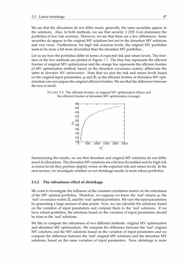
3.3. Linear shrinkage 47
We see that the allocations do not differ much; generally, the same securities appear inthe solutions. Also, in both methods, we see that security 2 (TJX Cos) dominates theportfolios of low risk aversion. However, we see that there are a few differences. Somesecurities do appear in the original MV solutions but not in the shrunken MV solutionsand vice versa. Furthermore, for high risk aversion levels, the original MV portfoliosseem to be more a bit more diversified than the shrunken MV portfolios.
Let us see how the portfolios differ in terms of expected risk and return levels. The fron-tiers of the two methods are plotted in Figure 3.3. The blue line represents the efficientfrontier of original MV optimization and the orange line represents the efficient frontierof MV optimization method, based on the shrunken covariance matrix; abbreviate thelatter to shrunken MV optimization. Note that we plot the risk and return levels basedon the original input parameters, µ and Σ, so the efficient frontier of shrunken MV opti-mization can not surpass the original efficient frontier. We see that the difference betweenthe two is small.
FIGURE 3.3: The efficient frontier of original MV optimization (blue) andthe efficient frontier of shrunken MV optimization (orange).
0 500 1000 1500 2000 2500
σ 20
10
12
14
16
18
20
22
24
26
28
µ0
Summarizing the results, we see that shrunken and original MV solutions do not differmuch in allocations. The shrunken MV solutions are a bit less diversified and for high riskaversion levels they perform slightly worse on the expected risk and return levels. In thenext section, we investigate whether or not shrinkage results in more robust portfolios.
3.3.2 The robustness effect of shrinkage
We want to investigate the influence of the constant correlation matrix on the robustnessof the MV optimal portfolios. Therefore, we suppose we know the ‘real’ returns µ, the‘real’ covariance matrix Σ, and the ‘real’ optimal portfolios. We vary the input parametersby generating a large amount of data points. Now, we can calculate the solutions, basedon the variation of input parameters and compare them to the ‘real’ solutions. If wehave robust portfolios, the solutions based on the variation of input parameters shouldbe close to the ‘real’ solutions.
We like to compare the robustness of two different methods: original MV optimizationand shrunken MV optimization. We compute the difference between the ‘real’ originalMV solutions and the MV solutions based on the variation of input parameters and wecompute the difference between the ‘real’ original MV solutions and the shrunken MVsolutions, based on the same variation of input parameters. Now, shrinkage is more
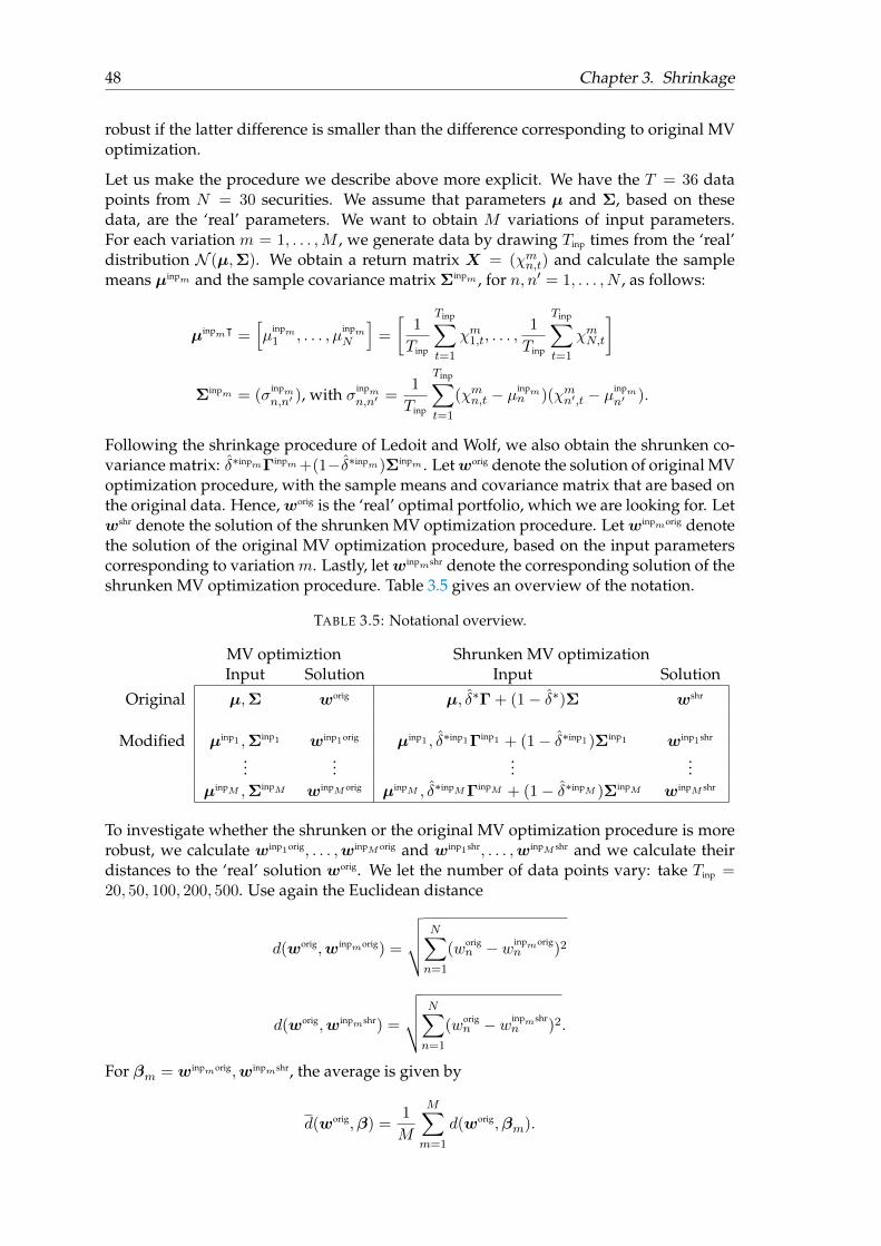
48 Chapter 3. Shrinkage
robust if the latter difference is smaller than the difference corresponding to original MVoptimization.
Let us make the procedure we describe above more explicit. We have the T = 36 datapoints from N = 30 securities. We assume that parameters µ and Σ, based on thesedata, are the ‘real’ parameters. We want to obtain M variations of input parameters.For each variation m = 1, . . . ,M , we generate data by drawing Tinp times from the ‘real’distribution N (µ,Σ). We obtain a return matrix X = (χmn,t) and calculate the samplemeans µinpm and the sample covariance matrix Σinpm , for n, n′ = 1, . . . , N , as follows:
µinpmᵀ =[µ
inpm1 , . . . , µ
inpmN
]=
[1
Tinp
Tinp∑t=1
χm1,t, . . . ,1
Tinp
Tinp∑t=1
χmN,t
]
Σinpm = (σinpmn,n′ ), with σinpm
n,n′ =1
Tinp
Tinp∑t=1
(χmn,t − µinpmn )(χmn′,t − µ
inpmn′ ).
Following the shrinkage procedure of Ledoit and Wolf, we also obtain the shrunken co-variance matrix: δ̂∗inpmΓinpm +(1−δ̂∗inpm)Σinpm . Letworig denote the solution of original MVoptimization procedure, with the sample means and covariance matrix that are based onthe original data. Hence,worig is the ‘real’ optimal portfolio, which we are looking for. Letwshr denote the solution of the shrunken MV optimization procedure. Letwinpmorig denotethe solution of the original MV optimization procedure, based on the input parameterscorresponding to variationm. Lastly, letwinpmshr denote the corresponding solution of theshrunken MV optimization procedure. Table 3.5 gives an overview of the notation.
TABLE 3.5: Notational overview.
MV optimiztion Shrunken MV optimizationInput Solution Input Solution
Original µ,Σ worig µ, δ̂∗Γ + (1− δ̂∗)Σ wshr
Modified µinp1 ,Σinp1 winp1orig µinp1 , δ̂∗inp1Γinp1 + (1− δ̂∗inp1)Σinp1 winp1shr
......
......
µinpM ,ΣinpM winpM orig µinpM , δ̂∗inpM ΓinpM + (1− δ̂∗inpM )ΣinpM winpM shr
To investigate whether the shrunken or the original MV optimization procedure is morerobust, we calculate winp1orig, . . . ,winpM orig and winp1shr, . . . ,winpM shr and we calculate theirdistances to the ‘real’ solution worig. We let the number of data points vary: take Tinp =20, 50, 100, 200, 500. Use again the Euclidean distance
d(worig,winpmorig) =
√√√√ N∑n=1
(worign − winpmorig
n )2
d(worig,winpmshr) =
√√√√ N∑n=1
(worign − winpmshr
n )2.
For βm = winpmorig,winpmshr, the average is given by
d(worig,β) =1
M
M∑m=1
d(worig,βm).
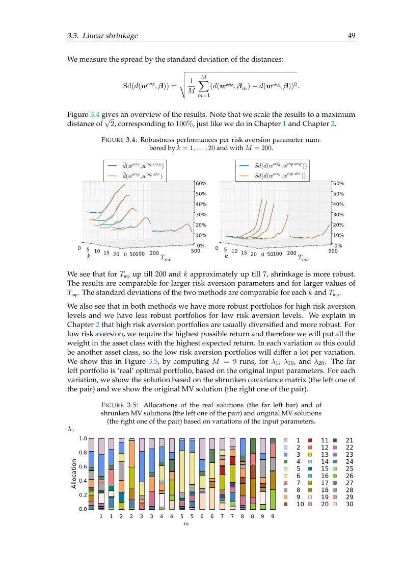
3.3. Linear shrinkage 49
We measure the spread by the standard deviation of the distances:
Sd(d(worig,β)) =
√√√√ 1
M
M∑m=1
(d(worig,βm)− d(worig,β))2.
Figure 3.4 gives an overview of the results. Note that we scale the results to a maximumdistance of
√2, corresponding to 100%, just like we do in Chapter 1 and Chapter 2.
FIGURE 3.4: Robustness performances per risk aversion parameter num-bered by k = 1, . . . , 20 and with M = 200.
k0 5 10 15 20
Tinp0 50100 200 500
0%
10%
20%
30%
40%
50%
60%
d(worig ,winp orig )
d(worig ,winp shr )
k0 5 10 15 20
Tinp0 50100 200 500
0%
10%
20%
30%
40%
50%
60%
Sd(d(worig ,winp orig ))
Sd(d(worig ,winp shr ))
We see that for Tinp up till 200 and k approximately up till 7, shrinkage is more robust.The results are comparable for larger risk aversion parameters and for larger values ofTinp. The standard deviations of the two methods are comparable for each k and Tinp.
We also see that in both methods we have more robust portfolios for high risk aversionlevels and we have less robust portfolios for low risk aversion levels. We explain inChapter 2 that high risk aversion portfolios are usually diversified and more robust. Forlow risk aversion, we require the highest possible return and therefore we will put all theweight in the asset class with the highest expected return. In each variation m this couldbe another asset class, so the low risk aversion portfolios will differ a lot per variation.We show this in Figure 3.5, by computing M = 9 runs, for λ1, λ10, and λ20. The farleft portfolio is ‘real’ optimal portfolio, based on the original input parameters. For eachvariation, we show the solution based on the shrunken covariance matrix (the left one ofthe pair) and we show the original MV solution (the right one of the pair).
FIGURE 3.5: Allocations of the real solutions (the far left bar) and ofshrunken MV solutions (the left one of the pair) and original MV solutions
(the right one of the pair) based on variations of the input parameters.λ1
1 1 2 2 3 3 4 4 5 5 6 6 7 7 8 8 9 9m
0.0
0.2
0.4
0.6
0.8
1.0
Allo
cati
on
12345678910
11121314151617181920
21222324252627282930
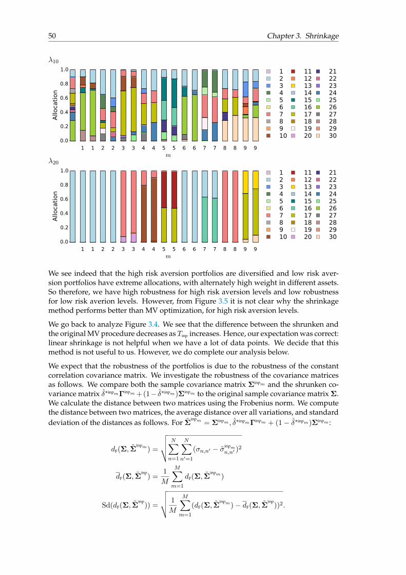
50 Chapter 3. Shrinkage
λ10
1 1 2 2 3 3 4 4 5 5 6 6 7 7 8 8 9 9m
0.0
0.2
0.4
0.6
0.8
1.0
Allo
cati
on
12345678910
11121314151617181920
21222324252627282930
λ20
1 1 2 2 3 3 4 4 5 5 6 6 7 7 8 8 9 9m
0.0
0.2
0.4
0.6
0.8
1.0
Allo
cati
on
12345678910
11121314151617181920
21222324252627282930
We see indeed that the high risk aversion portfolios are diversified and low risk aver-sion portfolios have extreme allocations, with alternately high weight in different assets.So therefore, we have high robustness for high risk aversion levels and low robustnessfor low risk averion levels. However, from Figure 3.5 it is not clear why the shrinkagemethod performs better than MV optimization, for high risk aversion levels.
We go back to analyze Figure 3.4. We see that the difference between the shrunken andthe original MV procedure decreases as Tinp increases. Hence, our expectation was correct:linear shrinkage is not helpful when we have a lot of data points. We decide that thismethod is not useful to us. However, we do complete our analysis below.
We expect that the robustness of the portfolios is due to the robustness of the constantcorrelation covariance matrix. We investigate the robustness of the covariance matricesas follows. We compare both the sample covariance matrix Σinpm and the shrunken co-variance matrix δ̂∗inpmΓinpm +(1− δ̂∗inpm)Σinpm to the original sample covariance matrix Σ.We calculate the distance between two matrices using the Frobenius norm. We computethe distance between two matrices, the average distance over all variations, and standarddeviation of the distances as follows. For Σ̃
inpm = Σinpm , δ̂∗inpmΓinpm + (1− δ̂∗inpm)Σinpm :
dF(Σ, Σ̃inpm) =
√√√√ N∑n=1
N∑n′=1
(σn,n′ − σ̃inpmn,n′ )
2
dF(Σ, Σ̃inp
) =1
M
M∑m=1
dF(Σ, Σ̃inpm)
Sd(dF(Σ, Σ̃inp
)) =
√√√√ 1
M
M∑m=1
(dF(Σ, Σ̃inpm)− dF(Σ, Σ̃
inp))2.
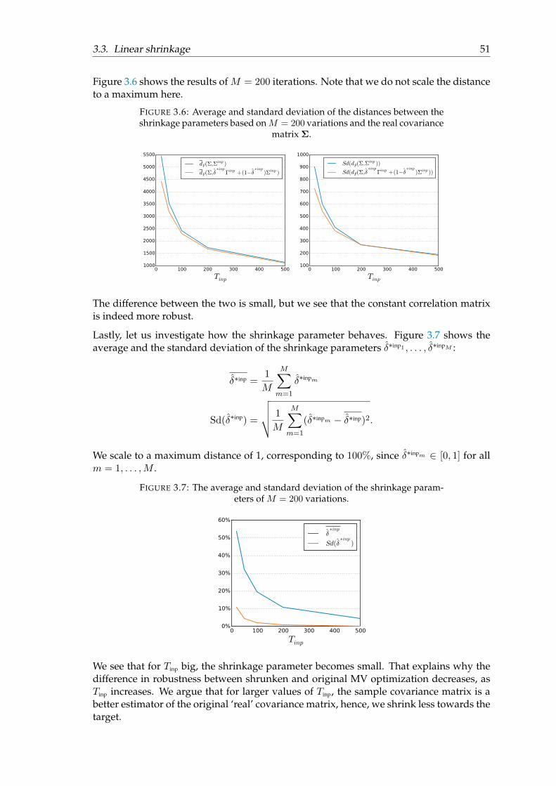
3.3. Linear shrinkage 51
Figure 3.6 shows the results of M = 200 iterations. Note that we do not scale the distanceto a maximum here.
FIGURE 3.6: Average and standard deviation of the distances between theshrinkage parameters based onM = 200 variations and the real covariance
matrix Σ.
0 100 200 300 400 500
Tinp
1000
1500
2000
2500
3000
3500
4000
4500
5000
5500
dF(Σ,Σinp )
dF(Σ,δ̂∗inp
Γinp +(1−δ̂∗inp
)Σinp )
0 100 200 300 400 500
Tinp
100
200
300
400
500
600
700
800
900
1000
Sd(dF(Σ,Σinp ))
Sd(dF(Σ,δ̂∗inp
Γinp +(1−δ̂∗inp
)Σinp ))
The difference between the two is small, but we see that the constant correlation matrixis indeed more robust.
Lastly, let us investigate how the shrinkage parameter behaves. Figure 3.7 shows theaverage and the standard deviation of the shrinkage parameters δ̂∗inp1 , . . . , δ̂∗inpM :
δ̂∗inp =1
M
M∑m=1
δ̂∗inpm
Sd(δ̂∗inp) =
√√√√ 1
M
M∑m=1
(δ̂∗inpm − δ̂∗inp)2.
We scale to a maximum distance of 1, corresponding to 100%, since δ̂∗inpm ∈ [0, 1] for allm = 1, . . . ,M .
FIGURE 3.7: The average and standard deviation of the shrinkage param-eters of M = 200 variations.
0 100 200 300 400 500
Tinp
0%
10%
20%
30%
40%
50%
60%
δ̂∗inp
Sd(δ̂∗inp
)
We see that for Tinp big, the shrinkage parameter becomes small. That explains why thedifference in robustness between shrunken and original MV optimization decreases, asTinp increases. We argue that for larger values of Tinp, the sample covariance matrix is abetter estimator of the original ‘real’ covariance matrix, hence, we shrink less towards thetarget.
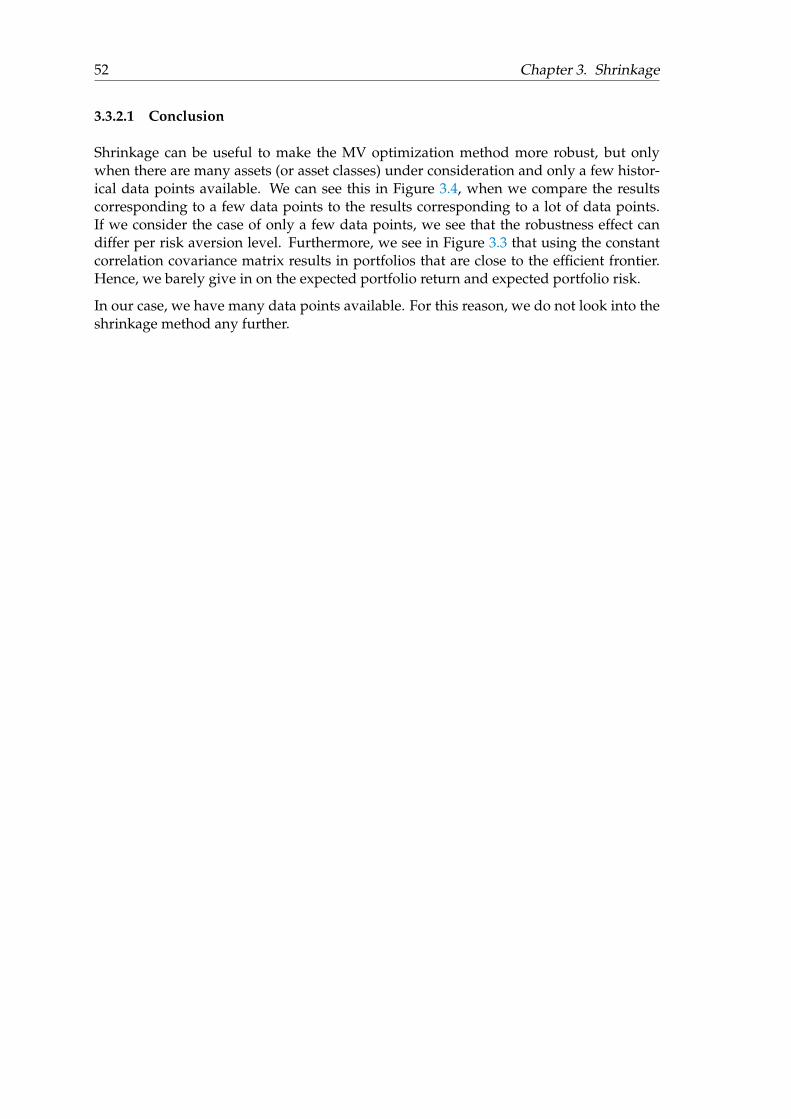
52 Chapter 3. Shrinkage
3.3.2.1 Conclusion
Shrinkage can be useful to make the MV optimization method more robust, but onlywhen there are many assets (or asset classes) under consideration and only a few histor-ical data points available. We can see this in Figure 3.4, when we compare the resultscorresponding to a few data points to the results corresponding to a lot of data points.If we consider the case of only a few data points, we see that the robustness effect candiffer per risk aversion level. Furthermore, we see in Figure 3.3 that using the constantcorrelation covariance matrix results in portfolios that are close to the efficient frontier.Hence, we barely give in on the expected portfolio return and expected portfolio risk.
In our case, we have many data points available. For this reason, we do not look into theshrinkage method any further.
53
Chapter 4
Maximum distance optimization
In this section, we develop a method to obtain a set of portfolios that are all near optimaland call this maximum distance optimization. Mean-Variance optimization provides uswith a range of portfolios that define the efficient frontier and now we want to knowwhat kind of portfolios lie closely beneath that efficient frontier. Can we invest in totallydifferent asset classes than the MV optimal portfolios do and still have a return and risklevel that are close to optimal?
We start with an MV optimal portfolio that corresponds to our risk aversion level andsearch for another portfolio, of which we require that it has approximately the same riskand return level, but is totally different in terms of allocations. Next, we search for an-other portfolio that also has approximately the same risk and return level, but again has adifferent set of weights than both the MV optimal portfolio and the firstly obtained port-folio. We continue this process and each time we obtain a different portfolio that is nearoptimal.
Given such a set of different portfolios that all meet the risk and return level require-ments, we can construct yet another portfolio, by taking a convex combination of theobtained portfolios. We prove that this convex combination portfolio also meets the riskand return level requirements. This means that this method provides us with uncount-able infinitely many solutions, which all have an acceptable risk and return level.
The idea is now that we can select a preferred portfolio from the near optimal portfoliosusing qualitative arguments that are potentially difficult to incorporate in the optimiza-tion process. For example, huge transaction costs might be involved by taking a positionin a certain asset class, or we have less confidence in the data used to model one of theasset classes. This practice suits well with how models are used: they are not assumed torepresent the absolute truth, but used as one source of input when making decisions.
Manually choosing any mix we like is an advantage, which we did not encounter in othermethods and as far as we know, it has not been published before. In resampling, for ex-ample, we do have some influence on the outcome by choosing values for the parameters,but the outcome for a certain risk aversion level is merely one portfolio. The method thatwe define in this chapter provides us with a whole scope of portfolios.
In this chapter, we first define the optimization program we like to solve, then we explainwhat Support Vector Machines are and show how Support Vector Machines enable usto implement the required optimization program. For this implementation, we use aheuristic method called Basin hopping and analyze the results.
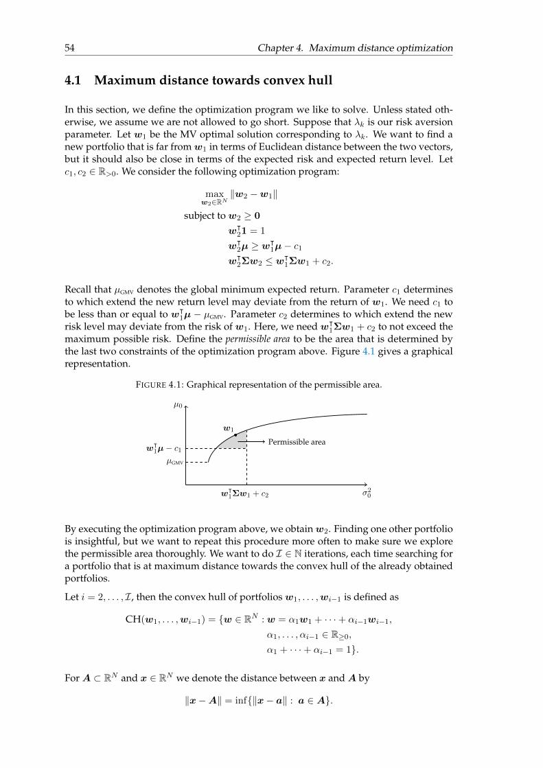
54 Chapter 4. Maximum distance optimization
4.1 Maximum distance towards convex hull
In this section, we define the optimization program we like to solve. Unless stated oth-erwise, we assume we are not allowed to go short. Suppose that λk is our risk aversionparameter. Let w1 be the MV optimal solution corresponding to λk. We want to find anew portfolio that is far fromw1 in terms of Euclidean distance between the two vectors,but it should also be close in terms of the expected risk and expected return level. Letc1, c2 ∈ R>0. We consider the following optimization program:
maxw2∈RN
‖w2 −w1‖
subject to w2 ≥ 0
wᵀ21 = 1
wᵀ2µ ≥ w
ᵀ1µ− c1
wᵀ2Σw2 ≤ wᵀ
1Σw1 + c2.
Recall that µGMV denotes the global minimum expected return. Parameter c1 determinesto which extend the new return level may deviate from the return of w1. We need c1 tobe less than or equal to wᵀ
1µ − µGMV. Parameter c2 determines to which extend the newrisk level may deviate from the risk of w1. Here, we need wᵀ
1Σw1 + c2 to not exceed themaximum possible risk. Define the permissible area to be the area that is determined bythe last two constraints of the optimization program above. Figure 4.1 gives a graphicalrepresentation.
FIGURE 4.1: Graphical representation of the permissible area.
σ20
µ0
w1
wᵀ1µ− c1
µGMV
wᵀ1Σw1 + c2
Permissible area
By executing the optimization program above, we obtainw2. Finding one other portfoliois insightful, but we want to repeat this procedure more often to make sure we explorethe permissible area thoroughly. We want to do I ∈ N iterations, each time searching fora portfolio that is at maximum distance towards the convex hull of the already obtainedportfolios.
Let i = 2, . . . , I, then the convex hull of portfolios w1, . . . ,wi−1 is defined as
CH(w1, . . . ,wi−1) = {w ∈ RN : w = α1w1 + · · ·+ αi−1wi−1,
α1, . . . , αi−1 ∈ R≥0,α1 + · · ·+ αi−1 = 1}.
ForA ⊂ RN and x ∈ RN we denote the distance between x andA by
‖x−A‖ = inf{‖x− a‖ : a ∈ A}.
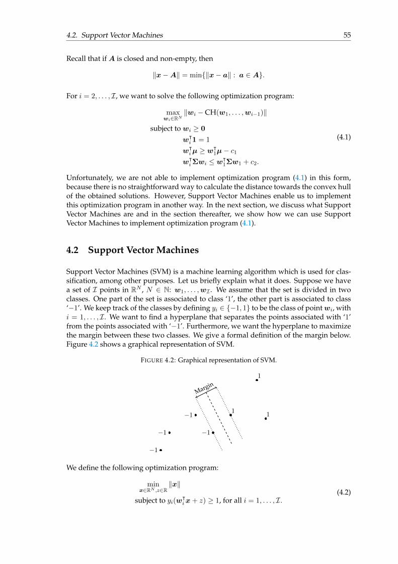
4.2. Support Vector Machines 55
Recall that ifA is closed and non-empty, then
‖x−A‖ = min{‖x− a‖ : a ∈ A}.
For i = 2, . . . , I, we want to solve the following optimization program:
maxwi∈RN
‖wi − CH(w1, . . . ,wi−1)‖
subject to wi ≥ 0
wᵀi 1 = 1
wᵀiµ ≥ w
ᵀ1µ− c1
wᵀiΣwi ≤ wᵀ
1Σw1 + c2.
(4.1)
Unfortunately, we are not able to implement optimization program (4.1) in this form,because there is no straightforward way to calculate the distance towards the convex hullof the obtained solutions. However, Support Vector Machines enable us to implementthis optimization program in another way. In the next section, we discuss what SupportVector Machines are and in the section thereafter, we show how we can use SupportVector Machines to implement optimization program (4.1).
4.2 Support Vector Machines
Support Vector Machines (SVM) is a machine learning algorithm which is used for clas-sification, among other purposes. Let us briefly explain what it does. Suppose we havea set of I points in RN , N ∈ N: w1, . . . ,wI . We assume that the set is divided in twoclasses. One part of the set is associated to class ‘1’, the other part is associated to class‘−1’. We keep track of the classes by defining yi ∈ {−1, 1} to be the class of pointwi, withi = 1, . . . , I. We want to find a hyperplane that separates the points associated with ‘1’from the points associated with ‘−1’. Furthermore, we want the hyperplane to maximizethe margin between these two classes. We give a formal definition of the margin below.Figure 4.2 shows a graphical representation of SVM.
FIGURE 4.2: Graphical representation of SVM.
1
1
1−1
−1
−1
−1
Margin
We define the following optimization program:
minx∈RN ,z∈R
‖x‖
subject to yi(wᵀix+ z) ≥ 1, for all i = 1, . . . , I.
(4.2)
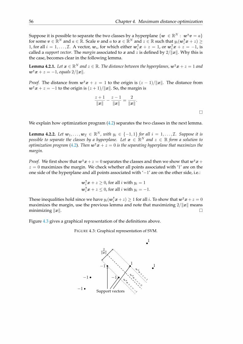
56 Chapter 4. Maximum distance optimization
Suppose it is possible to separate the two classes by a hyperplane {w ∈ RN : wᵀv = a}for some v ∈ RN and a ∈ R. Scale v and a to x ∈ RN and z ∈ R such that yi(w
ᵀix+ z) ≥
1, for all i = 1, . . . , I. A vector, wi, for which either wᵀix + z = 1, or wᵀ
ix + z = −1, iscalled a support vector. The margin associated to x and z is defined by 2/‖x‖. Why this isthe case, becomes clear in the following lemma.
Lemma 4.2.1. Let x ∈ RN and z ∈ R. The distance between the hyperplanes,wᵀx+ z = 1 andwᵀx+ z = −1, equals 2/‖x‖.
Proof. The distance from wᵀx + z = 1 to the origin is (z − 1)/‖x‖. The distance fromwᵀx+ z = −1 to the origin is (z + 1)/‖x‖. So, the margin is
z + 1
‖x‖− z − 1
‖x‖=
2
‖x‖.
We explain how optimization program (4.2) separates the two classes in the next lemma.
Lemma 4.2.2. Let w1, . . . ,wI ∈ RN , with yi ∈ {−1, 1} for all i = 1, . . . , I. Suppose it ispossible to separate the classes by a hyperplane. Let x ∈ RN and z ∈ R form a solution tooptimization program (4.2). Then wᵀx+ z = 0 is the separating hyperplane that maximizes themargin.
Proof. We first show thatwᵀx+ z = 0 separates the classes and then we show thatwᵀx+z = 0 maximizes the margin. We check whether all points associated with ‘1’ are on theone side of the hyperplane and all points associated with ‘−1’ are on the other side, i.e.:
wᵀix+ z ≥ 0, for all i with yi = 1
wᵀix+ z ≤ 0, for all i with yi = −1.
These inequalities hold since we have yi(wᵀix+ z) ≥ 1 for all i. To show thatwᵀx+ z = 0
maximizes the margin, use the previous lemma and note that maximizing 2/‖x‖ meansminimizing ‖x‖.
Figure 4.3 gives a graphical representation of the definitions above.
FIGURE 4.3: Graphical representation of SVM.
1
1
1−1
−1
−1
−1w ᵀ
x+z=0
w ᵀx+z=1w ᵀ
x+z=−1
2‖x‖
Support vectors
4.3. Formulation of maximum distance optimization 57
4.3 Formulation of maximum distance optimization
We make the following connection of optimization program (4.1) to SVM. Again, we havew1 as the MV optimal portfolio corresponding to our risk aversion parameter. We wantto find a new portfoliow2 that is far fromw1 in terms of the Euclidean distance betweenthe two vectors but still in the permissible area determined by c1 and c2. Let y1 = 1 andy2 = −1. Then we search for w2 such that
minx2,w2∈RN
z2∈R
‖x2‖
subject to w2 ≥ 0
wᵀ21 = 1
wᵀ2µ ≥ w
ᵀ1µ− c1
wᵀ2Σw2 ≤ wᵀ
1Σw1 + c2
y1(wᵀ1x2 + z2) ≥ 1
y2(wᵀ2x2 + z2) ≥ 1.
Again, let I ∈ N be the total number of portfolios that we want to obtain. Althoughw1 is obtained by executing the MV optimization program, we consider w1 as the resultof the ‘first iteration’, for notational purposes. For iteration i = 2, we obtain w2 fromthe optimization program above and for iteration i = 2, . . . , I, we search for solution wi
such that it is at maximum distance from the already obtained portfolios, w1, . . . ,wi−1.We generalize the optimization program above for iteration i = 2, . . . , I.
Definition 4.3.1. Let w1 be the MV optimal solution corresponding to our risk aversionparameter. For iteration i = 2, . . . , I, we have already obtained solutions w1, . . . ,wi−1.Let yi′ = 1 for all i′ = 1, . . . , i − 1 and let yi = −1. We define the following optimizationprogram and call it maximum distance optimization (MDO):
minxi,wi∈RN
zi∈R
‖xi‖
subject to wi ≥ 0
wᵀi 1 = 1
wᵀiµ ≥ w
ᵀ1µ− c1
wᵀiΣwi ≤ wᵀ
1Σw1 + c2
yi′(wᵀi′xi + zi) ≥ 1, for all i′ = 1, . . . , i.
(4.3)
We define solutions of MDO to be maximum distance portfolios. Note that since we considerw1 to be the solution of the first iteration, w1 is also a maximum distance portfolio. LetI ∈ N and w1, . . . ,wI be maximum distance portfolios. Also, let α1, . . . , αI ∈ R≥0, withα1+· · ·+αI = 1. Then we define the portfolio α1w1+· · ·+αIwI to be a convex combinationportfolio.
In Section 4.4, we show that we can implement optimization program (4.3) using a heuris-tic method, however, does it solve our initial optimization program (4.1)? We prove twotheorems. Theorem 4.3.2 shows that (4.1) and (4.3) are equivalent and in Theorem 4.3.3,we show that any convex combination portfolio lies in the permissible area.
58 Chapter 4. Maximum distance optimization
Theorem 4.3.2. Optimization programs, (4.1) and (4.3), are equivalent. That is, if xi, wi,zi are optimal for (4.3), then wi is optimal for (4.1) and if wi is optimal for (4.1) and ‖wi −CH(w1, . . . ,wi−1)‖ > 0, then there exists xi and zi such that xi, wi, zi are optimal for (4.3).
Proof. Let λk be our risk aversion parameter and let w1, . . . ,wi−1 be the already ob-tained portfolios. Suppose that for iteration i, wCH is optimal for (4.1), with ‖wCH −CH(w1, . . . ,wi−1)‖ > 0. We show that wCH is also optimal for (4.3). Suppose that wMDO,xMDO, zMDO form a (not necessarily optimal) solution to (4.3), that is, they satisfy the con-straints of (4.3). Let HMDO be the corresponding hyperplane: HMDO = {w : wᵀxMDO +zMDO = 1}, and H−MDO the corresponding halfspace: H−MDO = {w : wᵀxMDO + zMDO ≥ 1}.Note that 2/‖xMDO‖ = ‖wMDO −HMDO‖ by Lemma 4.2.1. Suppose that
‖wMDO −HMDO‖ > ‖wCH − CH(w1, . . . ,wi−1)‖.
Then,
‖wMDO − CH(w1, . . . ,wi−1)‖ ≥ ‖wMDO −HMDO‖ > ‖wCH − CH(w1, . . . ,wi−1)‖
since CH(w1, . . . ,wi−1) ⊆ H−MDO. But this contradicts with wCH being optimal for (4.1).Hence, ‖wMDO−HMDO‖ ≤ ‖wCH−CH(w1, . . . ,wi−1)‖ and therefore any optimal solutionfor (4.1) is an optimal solution to (4.3).
For the second part, we give a graphical representation in Figure 4.4, to help understandthe arguments. Suppose that for iteration i, wMDO, xMDO, zMDO form an optimal solutionto (4.3), with hyperplane HMDO = {w : wᵀxMDO + zMDO = 1} and halfspace H−MDO ={w : wᵀxMDO + zMDO ≥ 1}. We show that wMDO is also optimal for (4.1). Let wCH a (notnecessarily optimal) solution to (4.1). Suppose that
‖wCH − CH(w1, . . . ,wi−1)‖ > ‖wMDO − CH(w1, . . . ,wi−1)‖.
Let w′CH ∈ CH(w1, . . . ,wi−1) be such that ‖wCH − w′CH‖ = ‖wCH − CH(w1, . . . ,wi−1)‖.Define a hyperplane HCH such that wCH − w′CH⊥HCH and w′CH ∈ HCH. We prove thatthe corresponding halfspace H−CH satisfies CH(w1, . . . ,wi−1) ⊆ H−CH. Suppose that thereis a point v ∈ CH(w1, . . . ,wi−1), such that v /∈ H−CH. We have αv + (1 − α)w′CH ∈CH(w1, . . . ,wi−1), for all α ∈ [0, 1], so
‖wCH − (αv + (1− α)w′CH)‖ ≥ ‖wCH −w′CH‖.
Rewrite this for α > 0 as
2〈wCH,w′CH〉 − 2〈wCH,v〉+ α〈v,v〉+ 2(1− α)〈v,w′CH〉+ (α− 2)〈w′CH,w
′CH〉 ≥ 0.
Let α→ 0, then we obtain:
〈wCH −w′CH,w′CH − v〉 ≥ 0.
On the other hand, since wCH −w′CH⊥HCH and v /∈H−CH, we have
〈wCH −w′CH,v −w′CH〉 > 0.
This gives a contradiction, hence such a v cannot exist. We find a hyperplane such thatwCH −w′CH⊥HCH, w′CH ∈HCH, and CH(w1, . . . ,wi−1) ⊆H−CH. We get
‖wCH − CH(w1, . . . ,wi−1)‖ = ‖wCH −w′CH‖ = ‖wCH −HCH‖.
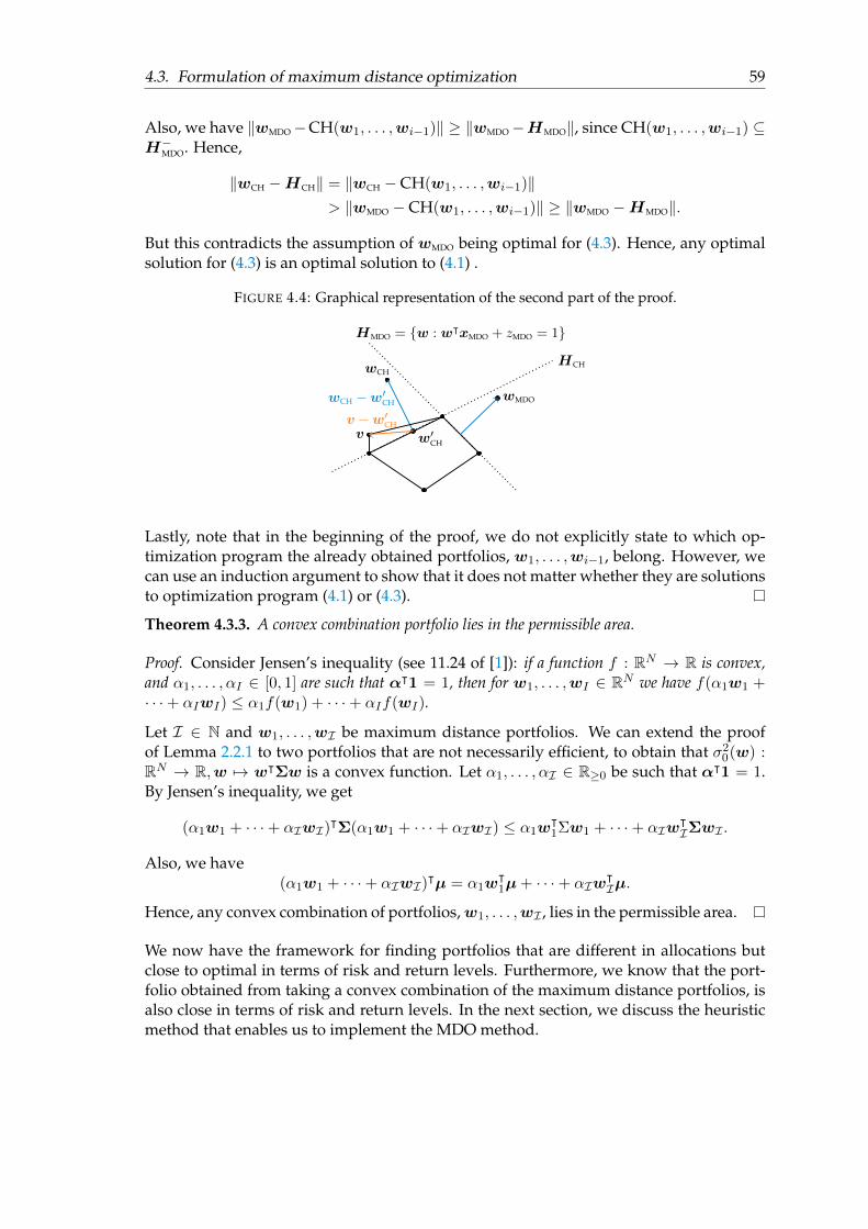
4.3. Formulation of maximum distance optimization 59
Also, we have ‖wMDO−CH(w1, . . . ,wi−1)‖ ≥ ‖wMDO−HMDO‖, since CH(w1, . . . ,wi−1) ⊆H−MDO. Hence,
‖wCH −HCH‖ = ‖wCH − CH(w1, . . . ,wi−1)‖> ‖wMDO − CH(w1, . . . ,wi−1)‖ ≥ ‖wMDO −HMDO‖.
But this contradicts the assumption of wMDO being optimal for (4.3). Hence, any optimalsolution for (4.3) is an optimal solution to (4.1) .
FIGURE 4.4: Graphical representation of the second part of the proof.
w′CH
wCH
wCH −w′CHwMDO
HCH
HMDO = {w : wᵀxMDO + zMDO = 1}
vv −w′CH
Lastly, note that in the beginning of the proof, we do not explicitly state to which op-timization program the already obtained portfolios, w1, . . . ,wi−1, belong. However, wecan use an induction argument to show that it does not matter whether they are solutionsto optimization program (4.1) or (4.3).
Theorem 4.3.3. A convex combination portfolio lies in the permissible area.
Proof. Consider Jensen’s inequality (see 11.24 of [1]): if a function f : RN → R is convex,and α1, . . . , αI ∈ [0, 1] are such that αᵀ1 = 1, then for w1, . . . ,wI ∈ RN we have f(α1w1 +· · ·+ αIwI) ≤ α1f(w1) + · · ·+ αIf(wI).
Let I ∈ N and w1, . . . ,wI be maximum distance portfolios. We can extend the proofof Lemma 2.2.1 to two portfolios that are not necessarily efficient, to obtain that σ20(w) :RN → R,w 7→ wᵀΣw is a convex function. Let α1, . . . , αI ∈ R≥0 be such that αᵀ1 = 1.By Jensen’s inequality, we get
(α1w1 + · · ·+ αIwI)ᵀΣ(α1w1 + · · ·+ αIwI) ≤ α1w
ᵀ1Σw1 + · · ·+ αIw
ᵀIΣwI .
Also, we have(α1w1 + · · ·+ αIwI)
ᵀµ = α1wᵀ1µ+ · · ·+ αIw
ᵀIµ.
Hence, any convex combination of portfolios,w1, . . . ,wI , lies in the permissible area.
We now have the framework for finding portfolios that are different in allocations butclose to optimal in terms of risk and return levels. Furthermore, we know that the port-folio obtained from taking a convex combination of the maximum distance portfolios, isalso close in terms of risk and return levels. In the next section, we discuss the heuristicmethod that enables us to implement the MDO method.
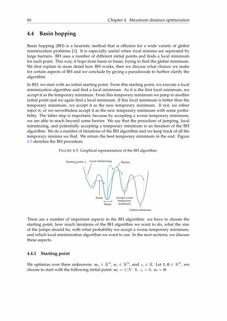
60 Chapter 4. Maximum distance optimization
4.4 Basin hopping
Basin hopping (BH) is a heuristic method that is efficient for a wide variety of globalminimization problems [4]. It is especially useful when local minima are separated bylarge barriers. BH uses a number of different initial points and finds a local minimumfor each point. This way, it hops from basin to basin, trying to find the global minimum.We first explain in more detail how BH works, then we discuss what choices we makefor certain aspects of BH and we conclude by giving a pseudocode to further clarify thealgorithm.
In BH, we start with an initial starting point. From this starting point, we execute a localminimization algorithm and find a local minimum. As it is the first local minimum, weaccept it as the temporary minimum. From this temporary minimum we jump to anotherinitial point and we again find a local minimum. If this local minimum is better than thetemporary minimum, we accept it as the new temporary minimum. If not, we eitherreject it, or we nevertheless accept it as the new temporary minimum with some proba-bility. The latter step is important, because by accepting a worse temporary minimum,we are able to reach beyond some barrier. We say that the procedure of jumping, localminimizing, and potentially accepting a temporary minimum is an iteration of the BHalgorithm. We do a number of iterations of the BH algorithm and we keep track of all thetemporary minima we find. We return the best temporary minimum in the end. Figure4.5 sketches the BH procedure.
FIGURE 4.5: Graphical representation of the BH algorithm.
Starting point Local minimizing
Jump Accept worsetemporaryminimum
Global minimum
Basin
Barrier
There are a number of important aspects in the BH algorithm: we have to choose thestarting point, how much iterations of the BH algorithm we want to do, what the sizeof the jumps should be, with what probability we accept a worse temporary minimum,and which local minimization algorithm we want to use. In the next sections, we discussthese aspects.
4.4.1 Starting point
We optimize over three unknowns: wi ∈ RN , xi ∈ RN , and zi ∈ R. Let 1,0 ∈ RN , wechoose to start with the following initial point: wi = 1/N · 1, zi = 0, xi = 0.
4.4. Basin hopping 61
4.4.2 Number of iterations
Let J denote the number of iterations of the BH algorithm. The greater the value of J ,the higher the probability of finding a global minimum. However, large J means morecomputation time. In Section 4.5, we work out an example and show the influence of thenumber of BH iterations on the computation time.
Note that if we obtain a local optimal solution instead of a global optimum, the solutionstill contributes to our search. We want to explore the region below the efficient frontierand we can explore it as thoroughly as we want, since we can choose I as large as wewant. Hence, if we obtain a large set of local optima, we can still thoroughly explore theregion below the efficient frontier.
4.4.3 Stepsize
The stepsize determines the size of the jumps. The stepsize should be comparable to thedifference between local minima of the function that is being optimized [4]. BH adjuststhe stepsize if necessary. A stepsize that is too small means that we may never jumpbeyond a barrier. A stepsize that is too big means that we may constantly jump over aglobal minimum. We use a stepsize of 1. The maximum distance between two portfoliosis√
2 and we argue that we rather make jumps that are too big than jumps that are toosmall.
4.4.4 Temperature
The probability that a worse temporary minimum is accepted, is determined by the objec-tive function and by a parameter called the temperature, τ . The probability of acceptanceis:
e−(Objective Function(new minimum)−Objective Function(old temporary minimum))/τ .
If the temperature is too big compared to the typical difference in objective function val-ues between local minima, we will almost always accept a worse minimum, perhaps atthe expense of not converging to a global minimum. If the temperature is too small, wemay never accept a worse minimum and therefore never reach beyond a barrier. Hence,the temperature should be comparable to the typical difference of the objective functionvalues between local minima.
We argue that in our case an appropriate value for τ depends on the number of assetclasses, N . Let n = 1, . . . , N and let wi, xi, zi form a local minimum. Let wn,i de-note the weight of asset class n of portfolio wi. We get wn,i = O(1/N). Let wCH
i ∈CH(w1, . . . ,wi−1) such that ‖wi − wCH
i ‖ = ‖wi − CH(w1, . . . ,wi−1)‖. Using Theorem4.3.2, we get
2/‖xi‖ = ‖wi −wCHi ‖ =
√√√√ N∑n=1
(wn,i − wCHn,i)
2 =
√√√√ N∑n=1
O(1/N)2 = O(1/√N).
So ‖xi‖ = O(√N). Let w′i, x
′i, z′i also form a local minimum. A typical difference of the
objective function values between these local minima is:
‖xi‖ − ‖x′i‖ = O(√N).
62 Chapter 4. Maximum distance optimization
Hence, for N not too big, we can choose τ =√N . However, for large N , it is better to
rescale our optimization problem as follows:
minxi,wi,zi
‖xi‖
subject to wi ≥ 0
wᵀi 1 = N
wᵀiµ ≥ w
ᵀ1µ− c1
wᵀiΣwi ≤ wᵀ
1Σw1 + c2.
yi′(wᵀi′xi + zi) ≥ 1, for all i′ = 1, . . . , i.
We get wn,i = O(1) and
2/‖xi‖ =
√√√√ N∑n=1
(wn,i − wCHn,i)
2 =
√√√√ N∑n=1
O(1)2 = O(√N).
So a typical difference of the objective function values between two local minima,wi andw′i, is:
‖xi‖ − ‖x′i‖ = O(1/√N).
We can choose τ = 1/√N .
4.4.5 Local minimization algorithm
We use a local minimization algorithm called Sequential Least Squares Programming.We do not go in to too much detail about how this algorithm works. We only note thatit has a stopping criterion of a maximum of 100 iterations and it tries to find an optimalfunction value up to a precision of 10−6.
4.4.6 Basin hopping pseudocode
We give the basin hopping algorithm in pseudocode.
(1) j = 0
(2) Xj = Starting point(3) Ytemp opt = Find local minimum around Xj
(4) while j < J do(5) Xj+1 = Jump from Ytemp opt to another point(6) Yj+1 = Find local minimum around Xj+1
(7) if Objective Function(Yj+1) < Objective Function(Ytemp opt) thenYtemp opt = Yj+1
Yglobal opt = Yj+1
(8) if Objective Function(Yj+1) ≮ Objective Function(Ytemp opt) then
with probability e−(Objective Function(Yj+1)−Objective Function(Ytemp opt))/τ
Ytemp opt = Yj+1
(9) j = j + 1
(10) return Yglobal opt
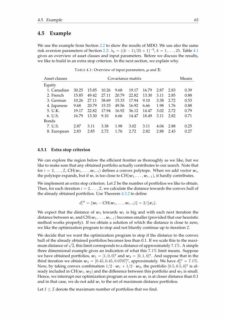
4.5. Example 63
4.5 Example
We use the example from Section 2.2 to show the results of MDO. We use also the samerisk aversion parameters of Section 2.2: λk = ((k − 1)/25 + 1)−9, k = 1, . . . , 25. Table 4.1gives an overview of asset classes and input parameters. Before we discuss the results,we like to build in an extra stop criterion. In the next section, we explain why.
TABLE 4.1: Overview of input parameters, µ and Σ.
Asset classes Covariance matrix Means
Equity1. Canadian 30.25 15.85 10.26 9.68 19.17 16.79 2.87 2.83 0.392. French 15.85 49.42 27.11 20.79 22.82 13.30 3.11 2.85 0.883. German 10.26 27.11 38.69 15.33 17.94 9.10 3.38 2.72 0.534. Japanese 9.68 20.79 15.33 49.56 16.92 6.66 1.98 1.76 0.885. U.K. 19.17 22.82 17.94 16.92 36.12 14.47 3.02 2.72 0.796. U.S. 16.79 13.30 9.10 6.66 14.47 18.49 3.11 2.82 0.71
Bonds7. U.S. 2.87 3.11 3.38 1.98 3.02 3.11 4.04 2.88 0.258. European 2.83 2.85 2.72 1.76 2.72 2.82 2.88 2.43 0.27
4.5.1 Extra stop criterion
We can explore the region below the efficient frontier as thoroughly as we like, but welike to make sure that any obtained portfolio actually contributes to our search. Note thatfor i = 2, . . . , I, CH(w1, . . . ,wi−1) defines a convex polytope. When we add vector wi,the polytope expands, but if wi is too close to CH(w1, . . . ,wi−1), it hardly contributes.
We implement an extra stop criterion. Let I be the number of portfolios we like to obtain.Then, for each iteration i = 2, . . . , I, we calculate the distance towards the convex hull ofthe already obtained portfolios. Use Theorem 4.3.2 to define
dCHi = ‖wi − CH(w1, . . . ,wi−1)‖ = 2/‖xi‖.
We expect that the distance of w2 towards w1 is big and with each next iteration thedistance betweenwi and CH(w1, . . . ,wi−1) becomes smaller (provided that our heuristicmethod works properly). If we obtain a solution of which the distance is close to zero,we like the optimization program to stop and not bluntly continue up to iteration I.
We decide that we want the optimization program to stop if the distance to the convexhull of the already obtained portfolios becomes less than 0.1. If we scale this to the maxi-mum distance of
√2, this limit corresponds to a distance of approximately 7.1%. A simple
three dimensional example gives an indication of what this 7.1% limit means. Supposewe have obtained portfolios, w1 = [1, 0, 0]ᵀ and w2 = [0, 1, 0]ᵀ. And suppose that in thethird iteration we obtain w3 = [0.45, 0.45, 0.0707]ᵀ, approximately. We have dCH
3 = 7.1%.Now, by taking convex combination 1/2 · w1 + 1/2 · w2, the portfolio [0.5, 0.5, 0]ᵀ is al-ready included in CH(w1,w2) and the difference between this portfolio and w3 is small.Hence, we interrupt our optimization program as soon aswi is at closer distance than 0.1and in that case, we do not add wi to the set of maximum distance portfolios.
Let I ≤ I denote the maximum number of portfolios that we find.
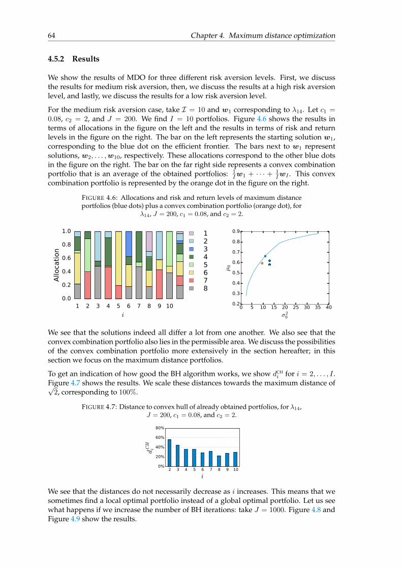
64 Chapter 4. Maximum distance optimization
4.5.2 Results
We show the results of MDO for three different risk aversion levels. First, we discussthe results for medium risk aversion, then, we discuss the results at a high risk aversionlevel, and lastly, we discuss the results for a low risk aversion level.
For the medium risk aversion case, take I = 10 and w1 corresponding to λ14. Let c1 =0.08, c2 = 2, and J = 200. We find I = 10 portfolios. Figure 4.6 shows the results interms of allocations in the figure on the left and the results in terms of risk and returnlevels in the figure on the right. The bar on the left represents the starting solution w1,corresponding to the blue dot on the efficient frontier. The bars next to w1 representsolutions, w2, . . . ,w10, respectively. These allocations correspond to the other blue dotsin the figure on the right. The bar on the far right side represents a convex combinationportfolio that is an average of the obtained portfolios: 1
Iw1 + · · · + 1IwI . This convex
combination portfolio is represented by the orange dot in the figure on the right.
FIGURE 4.6: Allocations and risk and return levels of maximum distanceportfolios (blue dots) plus a convex combination portfolio (orange dot), for
λ14, J = 200, c1 = 0.08, and c2 = 2.
1 2 3 4 5 6 7 8 9 10
i
0.0
0.2
0.4
0.6
0.8
1.0
Allo
cati
on
12345678
0 5 10 15 20 25 30 35 40
σ20
0.2
0.3
0.4
0.5
0.6
0.7
0.8
0.9µ
0
We see that the solutions indeed all differ a lot from one another. We also see that theconvex combination portfolio also lies in the permissible area. We discuss the possibilitiesof the convex combination portfolio more extensively in the section hereafter; in thissection we focus on the maximum distance portfolios.
To get an indication of how good the BH algorithm works, we show dCHi for i = 2, . . . , I .
Figure 4.7 shows the results. We scale these distances towards the maximum distance of√2, corresponding to 100%.
FIGURE 4.7: Distance to convex hull of already obtained portfolios, for λ14,J = 200, c1 = 0.08, and c2 = 2.
2 3 4 5 6 7 8 9 10
i
0%
20%
40%
60%
80%
dCH
i
We see that the distances do not necessarily decrease as i increases. This means that wesometimes find a local optimal portfolio instead of a global optimal portfolio. Let us seewhat happens if we increase the number of BH iterations: take J = 1000. Figure 4.8 andFigure 4.9 show the results.
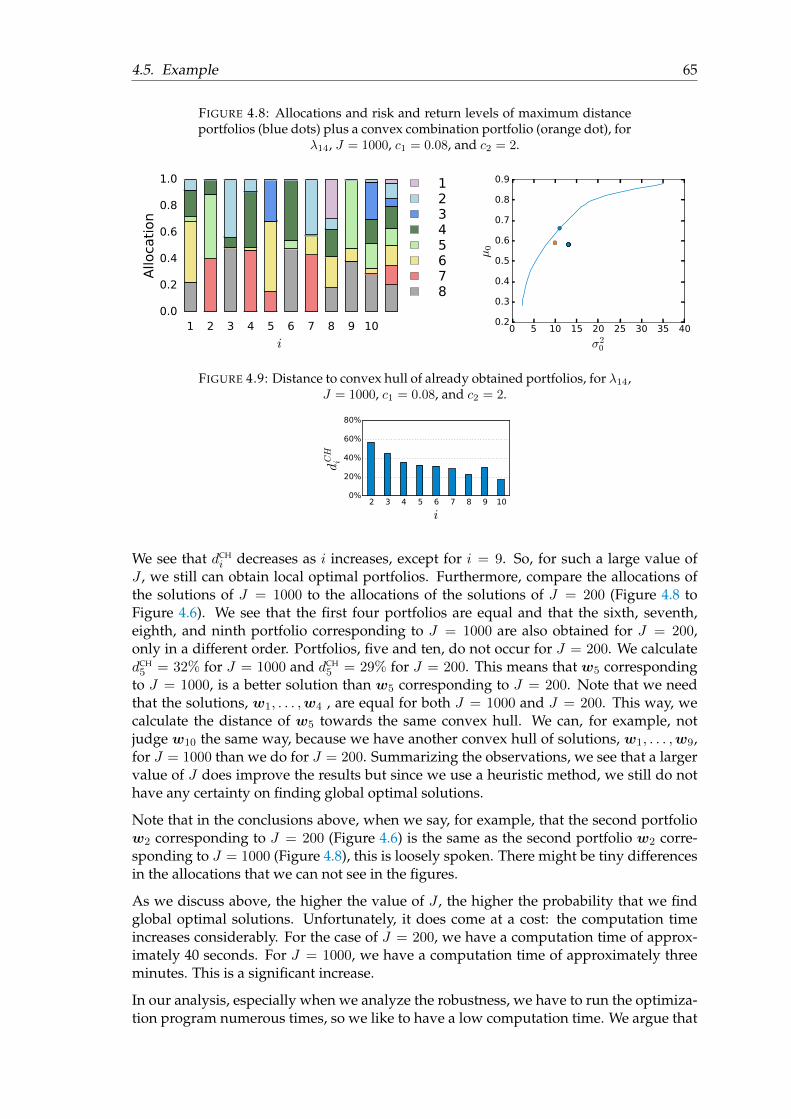
4.5. Example 65
FIGURE 4.8: Allocations and risk and return levels of maximum distanceportfolios (blue dots) plus a convex combination portfolio (orange dot), for
λ14, J = 1000, c1 = 0.08, and c2 = 2.
1 2 3 4 5 6 7 8 9 10
i
0.0
0.2
0.4
0.6
0.8
1.0
Allo
cati
on
12345678
0 5 10 15 20 25 30 35 40
σ20
0.2
0.3
0.4
0.5
0.6
0.7
0.8
0.9
µ0
FIGURE 4.9: Distance to convex hull of already obtained portfolios, for λ14,J = 1000, c1 = 0.08, and c2 = 2.
2 3 4 5 6 7 8 9 10
i
0%
20%
40%
60%
80%
dCH
i
We see that dCHi decreases as i increases, except for i = 9. So, for such a large value of
J , we still can obtain local optimal portfolios. Furthermore, compare the allocations ofthe solutions of J = 1000 to the allocations of the solutions of J = 200 (Figure 4.8 toFigure 4.6). We see that the first four portfolios are equal and that the sixth, seventh,eighth, and ninth portfolio corresponding to J = 1000 are also obtained for J = 200,only in a different order. Portfolios, five and ten, do not occur for J = 200. We calculatedCH5 = 32% for J = 1000 and dCH
5 = 29% for J = 200. This means that w5 correspondingto J = 1000, is a better solution than w5 corresponding to J = 200. Note that we needthat the solutions, w1, . . . ,w4 , are equal for both J = 1000 and J = 200. This way, wecalculate the distance of w5 towards the same convex hull. We can, for example, notjudge w10 the same way, because we have another convex hull of solutions, w1, . . . ,w9,for J = 1000 than we do for J = 200. Summarizing the observations, we see that a largervalue of J does improve the results but since we use a heuristic method, we still do nothave any certainty on finding global optimal solutions.
Note that in the conclusions above, when we say, for example, that the second portfoliow2 corresponding to J = 200 (Figure 4.6) is the same as the second portfolio w2 corre-sponding to J = 1000 (Figure 4.8), this is loosely spoken. There might be tiny differencesin the allocations that we can not see in the figures.
As we discuss above, the higher the value of J , the higher the probability that we findglobal optimal solutions. Unfortunately, it does come at a cost: the computation timeincreases considerably. For the case of J = 200, we have a computation time of approx-imately 40 seconds. For J = 1000, we have a computation time of approximately threeminutes. This is a significant increase.
In our analysis, especially when we analyze the robustness, we have to run the optimiza-tion program numerous times, so we like to have a low computation time. We argue that
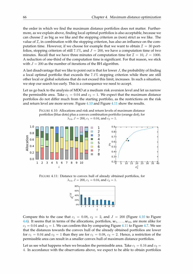
66 Chapter 4. Maximum distance optimization
the order in which we find the maximum distance portfolios does not matter. Further-more, as we explain above, finding local optimal portfolios is also acceptable, because wecan choose I as big as we like and the stopping criterion as (non) strict as we like. Thevalue of I, in combination with the stopping criterion, has also an influence on the com-putation time. However, if we choose for example that we want to obtain I = 30 port-folios, stopping criterion of still 7.1%, and J = 200, we have a computation time of twominutes. Recall that we have three minutes of computation time for I = 10, J = 1000.A reduction of one-third of the computation time is significant. For that reason, we stickwith J = 200 as the number of iterations of the BH algorithm.
A last disadvantage that we like to point out is that for lower J , the probability of findinga local optimal portfolio that exceeds the 7.1% stopping criterion while there are stillother local or global solutions that do not exceed this limit, increases. In such a situation,we stop our search too early. This is a consequence we need to accept.
Let us go back to the analysis of MDO at a medium risk aversion level and let us narrowthe permissible area. Take c1 = 0.04 and c2 = 1. We expect that the maximum distanceportfolios do not differ much from the starting portfolio, as the restrictions on the riskand return level are more severe. Figure 4.10 and Figure 4.11 show the results.
FIGURE 4.10: Allocations and risk and return levels of maximum distanceportfolios (blue dots) plus a convex combination portfolio (orange dot), for
λ14, J = 200, c1 = 0.04, and c2 = 1.
1 2 3 4 5 6 7 8 9 10
i
0.0
0.2
0.4
0.6
0.8
1.0
Allo
cati
on
12345678
0 5 10 15 20 25 30 35 40
σ20
0.2
0.3
0.4
0.5
0.6
0.7
0.8
0.9
µ0
FIGURE 4.11: Distance to convex hull of already obtained portfolios, forλ14, J = 200, c1 = 0.04, and c2 = 1.
2 3 4 5 6 7 8 9 10
i
0%
20%
40%
60%
80%
dCH
i
Compare this to the case that c1 = 0.08, c2 = 2, and J = 200 (Figure 4.10 to Figure4.6). It seems that in terms of the allocations, portfolios, w1, . . . ,w10, are more alike forc1 = 0.04 and c2 = 1. We can confirm this by comparing Figure 4.11 to Figure 4.7. We seethat the distances towards the convex hull of the already obtained portfolios are lowerfor c1 = 0.04 and c2 = 1 than they are for c1 = 0.08, c2 = 2. Hence, a restriction of thepermissible area can result in a smaller convex hull of maximum distance portfolios.
Let us see what happens when we broaden the permissible area. Take c1 = 0.16 and c2 =4. In accordance with the observations above, we expect to be able to obtain portfolios
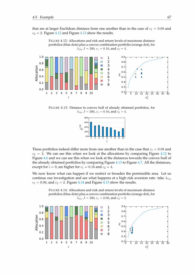
4.5. Example 67
that are at larger Euclidean distance from one another than in the case of c1 = 0.08 andc2 = 2. Figure 4.12 and Figure 4.13 show the results.
FIGURE 4.12: Allocations and risk and return levels of maximum distanceportfolios (blue dots) plus a convex combination portfolio (orange dot), for
λ14, J = 200, c1 = 0.16, and c2 = 4.
1 2 3 4 5 6 7 8 9 10
i
0.0
0.2
0.4
0.6
0.8
1.0
Allo
cati
on
12345678
0 5 10 15 20 25 30 35 40
σ20
0.2
0.3
0.4
0.5
0.6
0.7
0.8
0.9
µ0
FIGURE 4.13: Distance to convex hull of already obtained portfolios, forλ14, J = 200, c1 = 0.16, and c2 = 4.
2 3 4 5 6 7 8 9 10
i
0%
20%
40%
60%
80%
dCH
i
These portfolios indeed differ more from one another than in the case that c1 = 0.08 andc2 = 2. We can see this when we look at the allocations by comparing Figure 4.12 toFigure 4.6 and we can see this when we look at the distances towards the convex hull ofthe already obtained portfolios by comparing Figure 4.13 to Figure 4.7. All the distances,except for i = 9, are higher for c1 = 0.16 and c2 = 4.
We now know what can happen if we restrict or broaden the permissible area. Let uscontinue our investigation and see what happens at a high risk aversion rate: take λ11,c1 = 0.08, and c2 = 2. Figure 4.14 and Figure 4.15 show the results.
FIGURE 4.14: Allocations and risk and return levels of maximum distanceportfolios (blue dots) plus a convex combination portfolio (orange dot), for
λ11, J = 200, c1 = 0.08, and c2 = 2.
1 2 3 4 5 6 7 8 9 10
i
0.0
0.2
0.4
0.6
0.8
1.0
Allo
cati
on
12345678
0 5 10 15 20 25 30 35 40
σ20
0.2
0.3
0.4
0.5
0.6
0.7
0.8
0.9
µ0
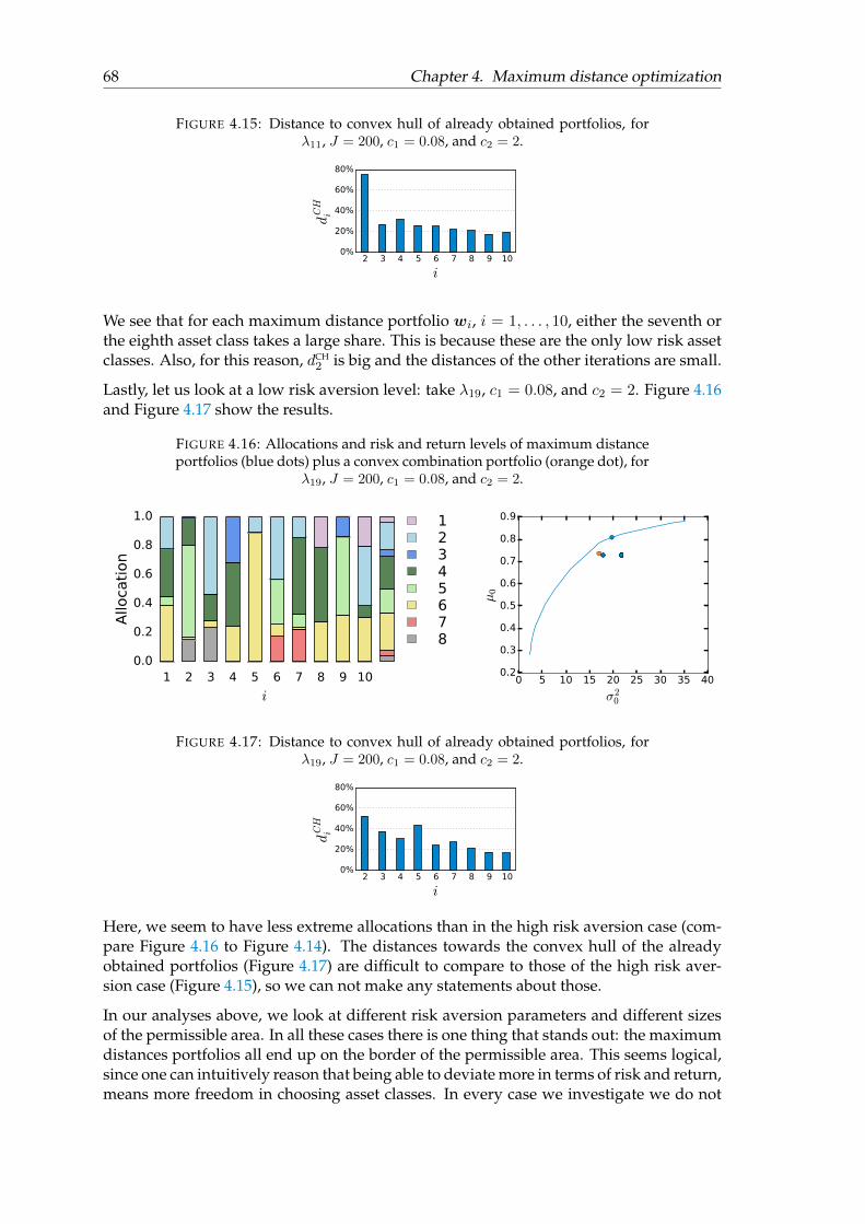
68 Chapter 4. Maximum distance optimization
FIGURE 4.15: Distance to convex hull of already obtained portfolios, forλ11, J = 200, c1 = 0.08, and c2 = 2.
2 3 4 5 6 7 8 9 10
i
0%
20%
40%
60%
80%
dCH
iWe see that for each maximum distance portfolio wi, i = 1, . . . , 10, either the seventh orthe eighth asset class takes a large share. This is because these are the only low risk assetclasses. Also, for this reason, dCH
2 is big and the distances of the other iterations are small.
Lastly, let us look at a low risk aversion level: take λ19, c1 = 0.08, and c2 = 2. Figure 4.16and Figure 4.17 show the results.
FIGURE 4.16: Allocations and risk and return levels of maximum distanceportfolios (blue dots) plus a convex combination portfolio (orange dot), for
λ19, J = 200, c1 = 0.08, and c2 = 2.
1 2 3 4 5 6 7 8 9 10
i
0.0
0.2
0.4
0.6
0.8
1.0
Allo
cati
on
12345678
0 5 10 15 20 25 30 35 40
σ20
0.2
0.3
0.4
0.5
0.6
0.7
0.8
0.9
µ0
FIGURE 4.17: Distance to convex hull of already obtained portfolios, forλ19, J = 200, c1 = 0.08, and c2 = 2.
2 3 4 5 6 7 8 9 10
i
0%
20%
40%
60%
80%
dCH
i
Here, we seem to have less extreme allocations than in the high risk aversion case (com-pare Figure 4.16 to Figure 4.14). The distances towards the convex hull of the alreadyobtained portfolios (Figure 4.17) are difficult to compare to those of the high risk aver-sion case (Figure 4.15), so we can not make any statements about those.
In our analyses above, we look at different risk aversion parameters and different sizesof the permissible area. In all these cases there is one thing that stands out: the maximumdistances portfolios all end up on the border of the permissible area. This seems logical,since one can intuitively reason that being able to deviate more in terms of risk and return,means more freedom in choosing asset classes. In every case we investigate we do not
4.5. Example 69
encounter a maximum distance portfolio that is not on the border of the permissible area,but nevertheless, our intuition misleads us, as we show in the next theorem.
Theorem 4.5.1. MDO has a solution that is on the border of the set determined by the constraints.
Proof. Consider the Bauer Maximum Principle (Theorem 7.69 from [1]): ‘If C is a compactconvex subset of a locally convex Hausdorff space, then every upper semicontinuous convex func-tion on C has a maximizer that is an extreme point.’. We use this theorem to show that we donot necessarily end up on the border of the permissible area.
Use Theorem 4.3.2 to see that we can use the formulation of optimization program (4.1).Let i = 2, . . . , I . Note that RN is a convex Hausdorff space and from Heine–Borel weknow that a subset of RN is compact if and only if it is closed and bounded. We have that{wi : wi ≥ 0} and {wi : wᵀ
iµ ≥ wᵀ1µ − c1} are closed half spaces and {wi : wᵀ
i 1 = 1}is a closed hyperplane, hence these sets are closed and convex. We know that {wi :wᵀiΣwi ≤ wᵀ
1Σw1+c2} is closed. It is also convex, since sublevel sets of convex functionsare convex. Furthermore, the intersection of closed convex sets is also closed and convex,hence the constraints of MDO form a convex set. Since we have wi such that wᵀ
i 1 = 1and wi ≥ 0 we know that the constraints also form a bounded set. Hence, the constraintsof (4.1) form a compact convex subset of a locally convex Hausdorff space.
Next, we show that the function RN → R : wi 7→ ‖wi − CH(w1, . . . ,wi−1)‖, is convexand continuous on RN . Let w′1,w
′2 ∈ RN (not to be confused with maximum distance
portfolios) and let α1, α2 ∈ R≥0, with α1 + α2 = 1. Let dw′1 ,dw′2 ∈ CH(w1, . . . ,wi−1) besuch that ∥∥w′1 − dw′1∥∥ =
∥∥w′1 − CH(w1, . . . ,wi−1)∥∥∥∥w′2 − dw′2∥∥ =
∥∥w′2 − CH(w1, . . . ,wi−1)∥∥ .
Then, α1dw′1 + α2dw′2 ∈ CH(w1, . . . ,wi−1) and we obtain∥∥α1w′1 + α2w
′2 − CH(w1, . . . ,wi−1)
∥∥ ≤ ∥∥α1w′1 + α2w
′2 − (α1dw′1 + α2dw′2)
∥∥≤ α1
∥∥w′1 − dw′1∥∥+ α2
∥∥w′2 − dw′2∥∥.Consider Theorem 7.24 from [1]: ‘In a finite dimensional vector space, every convex functionis continuous on the relative interior of its domain.’. We have RN as the relative interior ofitself, hence RN → R : wi 7→ ‖wi − CH(w1, . . . ,wi−1)‖ is continuous on RN .
Apply the Bauer Maximum Principle to optimization program (4.1). So, there is an ex-treme point of the following set:
{wi ∈ RN : wi ≥ 0, wᵀi 1 = 1, wᵀ
iµ ≥ wᵀ1µ− c1, w
ᵀiΣwi ≤ wᵀ
1Σw1 + c2}
that is a solution to (4.1).
We make the following remark. Theorem 4.5.1 implies that a solution of MDO is notnecessarily on the border of the permissible area. To see this, suppose thatwi is a solutionof MDO with wi ≥ 0 and wᵀ
i 1 = 1. Then, the conditions on the risk and return level arenot necessarily met with equality, hence wi does not necessarily lies on the border of thepermissible area.
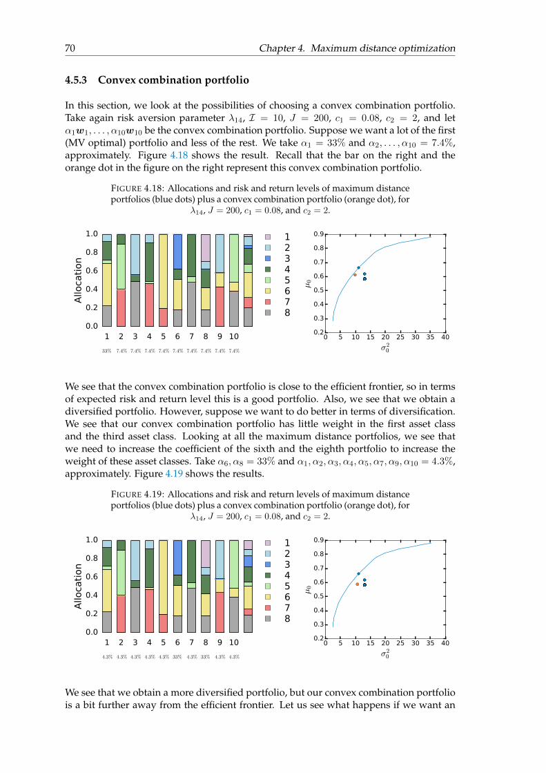
70 Chapter 4. Maximum distance optimization
4.5.3 Convex combination portfolio
In this section, we look at the possibilities of choosing a convex combination portfolio.Take again risk aversion parameter λ14, I = 10, J = 200, c1 = 0.08, c2 = 2, and letα1w1, . . . , α10w10 be the convex combination portfolio. Suppose we want a lot of the first(MV optimal) portfolio and less of the rest. We take α1 = 33% and α2, . . . , α10 = 7.4%,approximately. Figure 4.18 shows the result. Recall that the bar on the right and theorange dot in the figure on the right represent this convex combination portfolio.
FIGURE 4.18: Allocations and risk and return levels of maximum distanceportfolios (blue dots) plus a convex combination portfolio (orange dot), for
λ14, J = 200, c1 = 0.08, and c2 = 2.
1 2 3 4 5 6 7 8 9 10
[0.33, 0.07, 0.07, 0.07, 0.07, 0.07, 0.07, 0.07, 0.07, 0.07]
0.0
0.2
0.4
0.6
0.8
1.0
Allo
cati
on
12345678
0.440.100.100.100.100.100.100.100.100.10
Reset
Reset frontier
0 5 10 15 20 25 30 35 40
σ20
0.2
0.3
0.4
0.5
0.6
0.7
0.8
0.9
µ0
33% 7.4% 7.4% 7.4% 7.4% 7.4% 7.4% 7.4% 7.4% 7.4%
We see that the convex combination portfolio is close to the efficient frontier, so in termsof expected risk and return level this is a good portfolio. Also, we see that we obtain adiversified portfolio. However, suppose we want to do better in terms of diversification.We see that our convex combination portfolio has little weight in the first asset classand the third asset class. Looking at all the maximum distance portfolios, we see thatwe need to increase the coefficient of the sixth and the eighth portfolio to increase theweight of these asset classes. Take α6, α8 = 33% and α1, α2, α3, α4, α5, α7, α9, α10 = 4.3%,approximately. Figure 4.19 shows the results.
FIGURE 4.19: Allocations and risk and return levels of maximum distanceportfolios (blue dots) plus a convex combination portfolio (orange dot), for
λ14, J = 200, c1 = 0.08, and c2 = 2.
1 2 3 4 5 6 7 8 9 10
[0.04, 0.04, 0.04, 0.04, 0.04, 0.33, 0.04, 0.33, 0.04, 0.04]
0.0
0.2
0.4
0.6
0.8
1.0
Allo
cati
on
12345678
0.100.100.100.100.100.760.100.760.100.10
Reset
Reset frontier
0 5 10 15 20 25 30 35 40
σ20
0.2
0.3
0.4
0.5
0.6
0.7
0.8
0.9
µ0
4.3% 4.3% 4.3% 4.3% 4.3% 33% 4.3% 33% 4.3% 4.3%
We see that we obtain a more diversified portfolio, but our convex combination portfoliois a bit further away from the efficient frontier. Let us see what happens if we want an
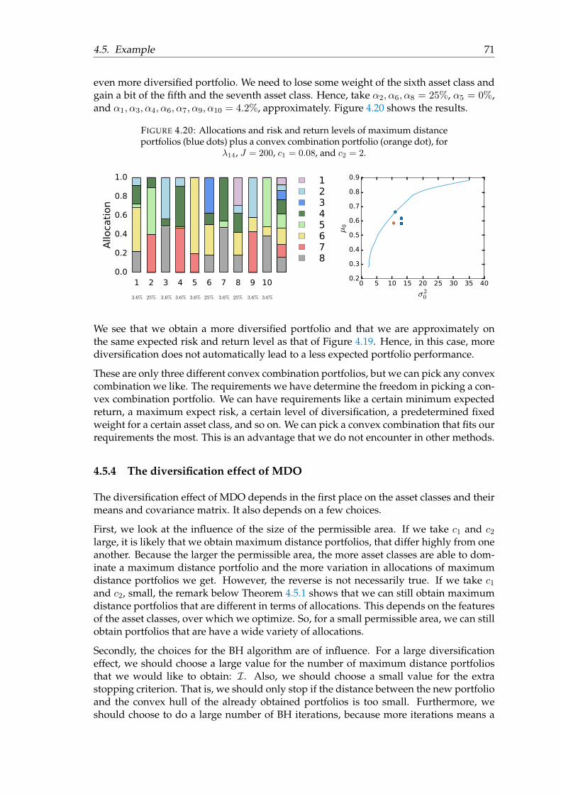
4.5. Example 71
even more diversified portfolio. We need to lose some weight of the sixth asset class andgain a bit of the fifth and the seventh asset class. Hence, take α2, α6, α8 = 25%, α5 = 0%,and α1, α3, α4, α6, α7, α9, α10 = 4.2%, approximately. Figure 4.20 shows the results.
FIGURE 4.20: Allocations and risk and return levels of maximum distanceportfolios (blue dots) plus a convex combination portfolio (orange dot), for
λ14, J = 200, c1 = 0.08, and c2 = 2.
1 2 3 4 5 6 7 8 9 10
[0.04, 0.25, 0.04, 0.04, 0.0, 0.25, 0.04, 0.25, 0.04, 0.04]
0.0
0.2
0.4
0.6
0.8
1.0
Allo
cati
on
12345678
0.050.320.050.050.000.320.050.320.050.05
Reset
Reset frontier
0 5 10 15 20 25 30 35 40
σ20
0.2
0.3
0.4
0.5
0.6
0.7
0.8
0.9
µ0
3.6% 25% 3.6% 3.6% 3.6% 25% 3.6% 25% 3.6% 3.6%
We see that we obtain a more diversified portfolio and that we are approximately onthe same expected risk and return level as that of Figure 4.19. Hence, in this case, morediversification does not automatically lead to a less expected portfolio performance.
These are only three different convex combination portfolios, but we can pick any convexcombination we like. The requirements we have determine the freedom in picking a con-vex combination portfolio. We can have requirements like a certain minimum expectedreturn, a maximum expect risk, a certain level of diversification, a predetermined fixedweight for a certain asset class, and so on. We can pick a convex combination that fits ourrequirements the most. This is an advantage that we do not encounter in other methods.
4.5.4 The diversification effect of MDO
The diversification effect of MDO depends in the first place on the asset classes and theirmeans and covariance matrix. It also depends on a few choices.
First, we look at the influence of the size of the permissible area. If we take c1 and c2large, it is likely that we obtain maximum distance portfolios, that differ highly from oneanother. Because the larger the permissible area, the more asset classes are able to dom-inate a maximum distance portfolio and the more variation in allocations of maximumdistance portfolios we get. However, the reverse is not necessarily true. If we take c1and c2, small, the remark below Theorem 4.5.1 shows that we can still obtain maximumdistance portfolios that are different in terms of allocations. This depends on the featuresof the asset classes, over which we optimize. So, for a small permissible area, we can stillobtain portfolios that are have a wide variety of allocations.
Secondly, the choices for the BH algorithm are of influence. For a large diversificationeffect, we should choose a large value for the number of maximum distance portfoliosthat we would like to obtain: I. Also, we should choose a small value for the extrastopping criterion. That is, we should only stop if the distance between the new portfolioand the convex hull of the already obtained portfolios is too small. Furthermore, weshould choose to do a large number of BH iterations, because more iterations means a
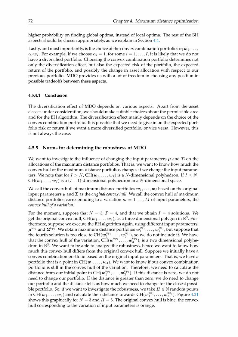
72 Chapter 4. Maximum distance optimization
higher probability on finding global optima, instead of local optima. The rest of the BHaspects should be chosen appropriately, as we explain in Section 4.4.
Lastly, and most importantly, is the choice of the convex combination portfolio: α1w1, . . . ,αIwI . For example, if we choose αi = 1, for some i = 1, . . . , I , it is likely that we do nothave a diversified portfolio. Choosing the convex combination portfolio determines notonly the diversification effect, but also the expected risk of the portfolio, the expectedreturn of the portfolio, and possibly the change in asset allocation with respect to ourprevious portfolio. MDO provides us with a lot of freedom in choosing any position inpossible tradeoffs between these aspects.
4.5.4.1 Conclusion
The diversification effect of MDO depends on various aspects. Apart from the assetclasses under consideration, we should make suitable choices about the permissible areaand for the BH algorithm. The diversification effect mainly depends on the choice of theconvex combination portfolio. It is possible that we need to give in on the expected port-folio risk or return if we want a more diversified portfolio, or vice versa. However, thisis not always the case.
4.5.5 Norms for determining the robustness of MDO
We want to investigate the influence of changing the input parameters µ and Σ on theallocations of the maximum distance portfolios. That is, we want to know how much theconvex hull of the maximum distance portfolios changes if we change the input parame-ters. We note that for I > N , CH(w1, . . . ,wI) is a N -dimensional polyhedron. If I ≤ N ,CH(w1, . . . ,wI) is a (I − 1)-dimensional polyhedron in a N -dimensional space.
We call the convex hull of maximum distance portfoliosw1, . . . ,wI based on the originalinput parameters µ and Σ as the original convex hull. We call the convex hull of maximumdistance portfolios corresponding to a variation m = 1, . . . ,M of input parameters, theconvex hull of a variation.
For the moment, suppose that N = 3, I = 4, and that we obtain I = 4 solutions. Weget the original convex hull, CH(w1, . . . ,w4), as a three dimensional polygon in R3. Fur-thermore, suppose we execute the BH algorithm again, using different input parameters:µinp1 and Σinp1 . We obtain maximum distance portfolioswinp1
1 , . . . ,winp14 , but suppose that
the fourth solution is too close to CH(winp11 , . . . ,w
inp13 ), so we do not include it. We have
that the convex hull of the variation, CH(winp11 , . . . ,w
inp13 ), is a two dimensional polyhe-
dron in R3. We want to be able to analyze the robustness, hence we want to know howmuch this convex hull differs from the original convex hull. Suppose we initially have aconvex combination portfolio based on the original input parameters. That is, we have aportfolio that is a point in CH(w1, . . . ,w4). We want to know if our convex combinationportfolio is still in the convex hull of the variation. Therefore, we need to calculate thedistance from our initial point to CH(w
inp11 , . . . ,w
inp13 ). If this distance is zero, we do not
need to change our portfolio. If the distance is greater than zero, we do need to changeour portfolio and the distance tells us how much we need to change for the closest possi-ble portfolio. So, if we want to investigate the robustness, we take H ∈ N random pointsin CH(w1, . . . ,w4) and calculate their distance towards CH(w
inp11 , . . . ,w
inp13 ). Figure 4.21
shows this graphically for N = 3 and H = 5. The original convex hull is blue, the convexhull corresponding to the variation of input parameters is orange.
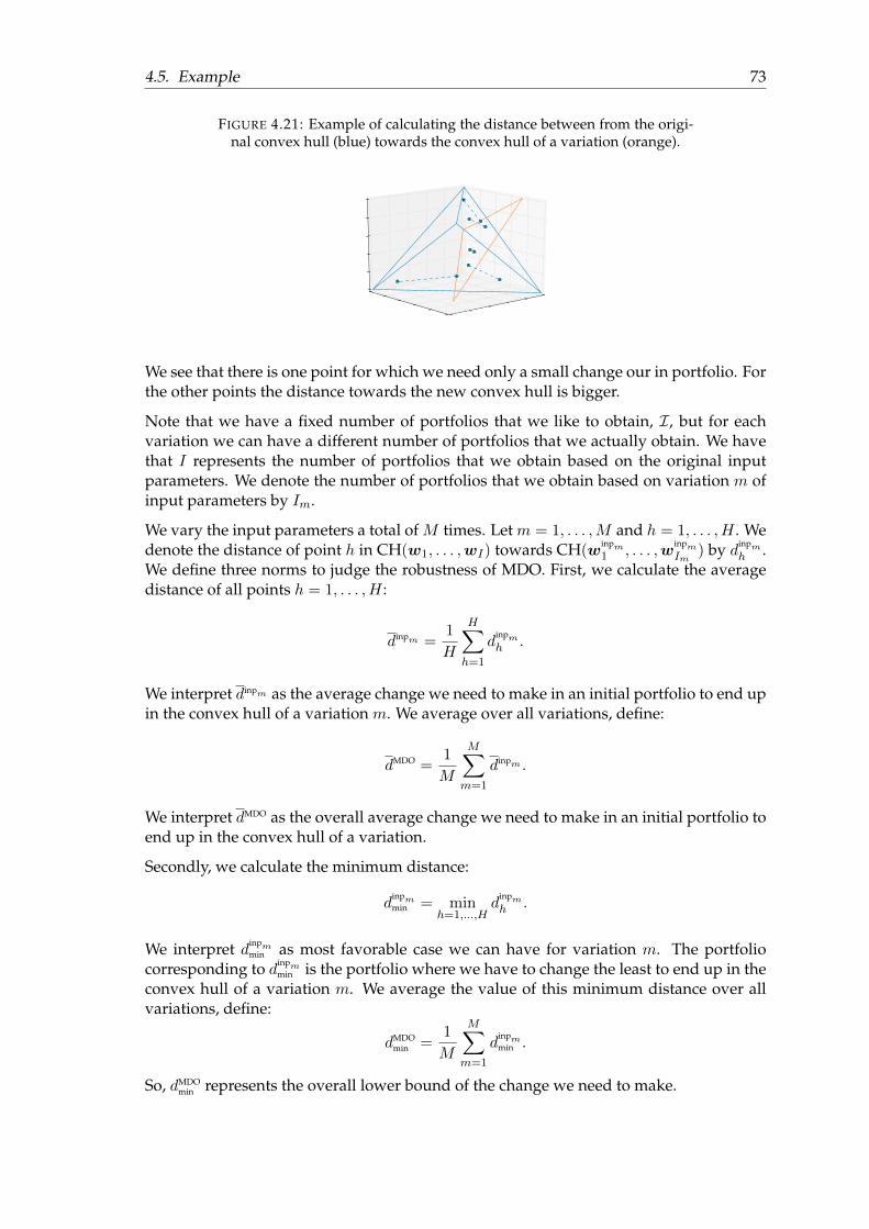
4.5. Example 73
FIGURE 4.21: Example of calculating the distance between from the origi-nal convex hull (blue) towards the convex hull of a variation (orange).
We see that there is one point for which we need only a small change our in portfolio. Forthe other points the distance towards the new convex hull is bigger.
Note that we have a fixed number of portfolios that we like to obtain, I, but for eachvariation we can have a different number of portfolios that we actually obtain. We havethat I represents the number of portfolios that we obtain based on the original inputparameters. We denote the number of portfolios that we obtain based on variation m ofinput parameters by Im.
We vary the input parameters a total of M times. Let m = 1, . . . ,M and h = 1, . . . ,H . Wedenote the distance of point h in CH(w1, . . . ,wI) towards CH(w
inpm1 , . . . ,w
inpmIm
) by dinpmh .
We define three norms to judge the robustness of MDO. First, we calculate the averagedistance of all points h = 1, . . . ,H :
dinpm =1
H
H∑h=1
dinpmh .
We interpret dinpm as the average change we need to make in an initial portfolio to end upin the convex hull of a variation m. We average over all variations, define:
dMDO =1
M
M∑m=1
dinpm .
We interpret dMDO as the overall average change we need to make in an initial portfolio toend up in the convex hull of a variation.
Secondly, we calculate the minimum distance:
dinpmmin = min
h=1,...,Hd
inpmh .
We interpret dinpmmin as most favorable case we can have for variation m. The portfolio
corresponding to dinpmmin is the portfolio where we have to change the least to end up in the
convex hull of a variation m. We average the value of this minimum distance over allvariations, define:
dMDOmin =
1
M
M∑m=1
dinpmmin .
So, dMDOmin represents the overall lower bound of the change we need to make.
74 Chapter 4. Maximum distance optimization
Lastly, we calculate the maximum distance:
dinpmmax = max
h=1,...,Hd
inpmh
We interpret dinpmmax as the most unfavorable case we can have. The portfolio corresponding
to dinpmmax is the portfolio for which we need to change the most to end up in the convex hull
of a variation m. We average this maximum distance over all variations, define:
dMDOmax =
1
M
M∑m=1
dinpmmax .
Then, dMDOmax represents the overall upper bound of the change we need to make.
We also define a norm to judge about the robustness of MV optimization (just like we doin Section 1). We calculate the difference between the MV optimal portfolio based on theoriginal input parameters and the MV optimal portfolio based on variation m:
‖w1 −winpm1 ‖.
This represents the change we need to make if we want to keep an MV optimal portfoliowith the same risk aversion level. We compute the average over all variations, define:
dMV =1
M
M∑m=1
‖w1 −winpm1 ‖.
So dMV represents the average change in MV optimal portfolios. Note that here, we use adifferent notation for the robustness of MV optimization than we do in Section 1.3.1 andSection 2.2.2, but the calculation is the same.
Note that we use different measures to judge the robustness: for MV optimization, weuse a straightforward measure, but for MDO, we use three less obvious measures. Weshould keep this in mind when we compare these norms.
4.5.6 The robustness effect of MDO
Now that we have norms to judge the robustness of MDO, let us look at our example.Use again risk aversion parameters λk = ((k − 1)/25 + 1)−9, k = 1, . . . , 25. We vary theinput parameters using Tinp drawings from N (µ,Σ), just as we do in Section 2.2.2. TakeM = 100 variations of input parameters, H = 200 distance calculations from points inthe original convex hull towards the convex hull of a variation, a permissible area corre-sponding to c1 = 0.08 and c2 = 2, and levels of input parameter deviation correspondingto Tinp = 200, 2000, 20000. We have that Tinp = 200 means that we are dealing with mod-ified input parameters, which highly differ from the original input parameters and thatTinp = 20000 means that the modified input parameters do not differ much.
Recall that dMV denotes the average change in MV optimal portfolios, hence, it representsthe robustness of MV optimization. Furthermore, for MDO, we have that dMDO denotesthe average change in convex combination portfolios, dMDO
min represents the (average) lowerbound of the change in a convex combination portfolio, and dMDO
min represents the (average)upper bound of the change in a convex combination portfolio.
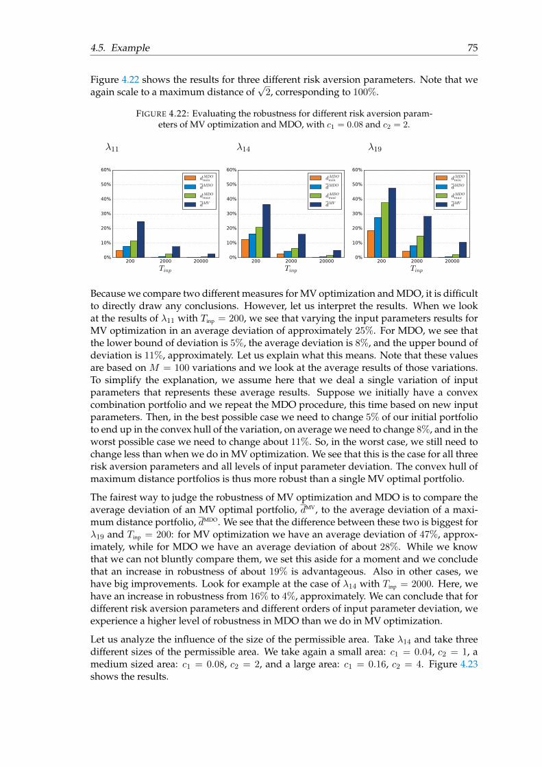
4.5. Example 75
Figure 4.22 shows the results for three different risk aversion parameters. Note that weagain scale to a maximum distance of
√2, corresponding to 100%.
FIGURE 4.22: Evaluating the robustness for different risk aversion param-eters of MV optimization and MDO, with c1 = 0.08 and c2 = 2.
200 2000 20000
Tinp
0%
10%
20%
30%
40%
50%
60%
dMDOmin
dMDO
dMDOmax
dMV
200 2000 20000
Tinp
0%
10%
20%
30%
40%
50%
60%
dMDOmin
dMDO
dMDOmax
dMV
200 2000 20000
Tinp
0%
10%
20%
30%
40%
50%
60%
dMDOmin
dMDO
dMDOmax
dMV
λ11 λ14 λ19
Because we compare two different measures for MV optimization and MDO, it is difficultto directly draw any conclusions. However, let us interpret the results. When we lookat the results of λ11 with Tinp = 200, we see that varying the input parameters results forMV optimization in an average deviation of approximately 25%. For MDO, we see thatthe lower bound of deviation is 5%, the average deviation is 8%, and the upper bound ofdeviation is 11%, approximately. Let us explain what this means. Note that these valuesare based on M = 100 variations and we look at the average results of those variations.To simplify the explanation, we assume here that we deal a single variation of inputparameters that represents these average results. Suppose we initially have a convexcombination portfolio and we repeat the MDO procedure, this time based on new inputparameters. Then, in the best possible case we need to change 5% of our initial portfolioto end up in the convex hull of the variation, on average we need to change 8%, and in theworst possible case we need to change about 11%. So, in the worst case, we still need tochange less than when we do in MV optimization. We see that this is the case for all threerisk aversion parameters and all levels of input parameter deviation. The convex hull ofmaximum distance portfolios is thus more robust than a single MV optimal portfolio.
The fairest way to judge the robustness of MV optimization and MDO is to compare theaverage deviation of an MV optimal portfolio, dMV, to the average deviation of a maxi-mum distance portfolio, dMDO. We see that the difference between these two is biggest forλ19 and Tinp = 200: for MV optimization we have an average deviation of 47%, approx-imately, while for MDO we have an average deviation of about 28%. While we knowthat we can not bluntly compare them, we set this aside for a moment and we concludethat an increase in robustness of about 19% is advantageous. Also in other cases, wehave big improvements. Look for example at the case of λ14 with Tinp = 2000. Here, wehave an increase in robustness from 16% to 4%, approximately. We can conclude that fordifferent risk aversion parameters and different orders of input parameter deviation, weexperience a higher level of robustness in MDO than we do in MV optimization.
Let us analyze the influence of the size of the permissible area. Take λ14 and take threedifferent sizes of the permissible area. We take again a small area: c1 = 0.04, c2 = 1, amedium sized area: c1 = 0.08, c2 = 2, and a large area: c1 = 0.16, c2 = 4. Figure 4.23shows the results.
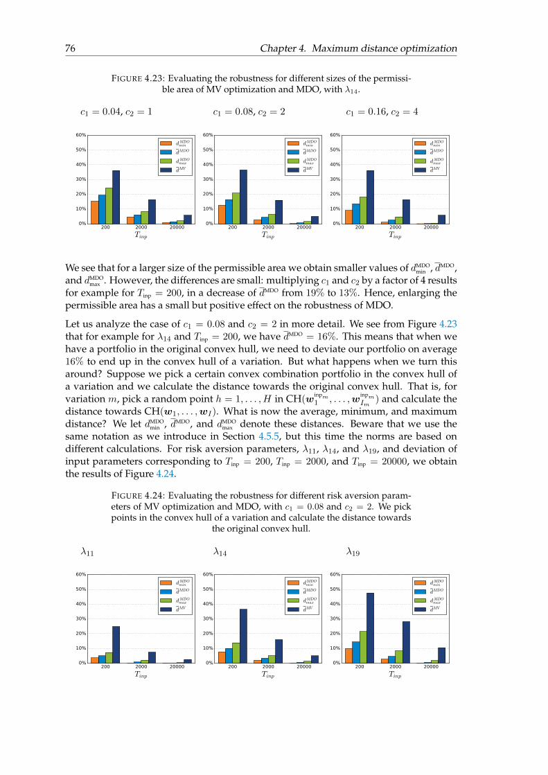
76 Chapter 4. Maximum distance optimization
FIGURE 4.23: Evaluating the robustness for different sizes of the permissi-ble area of MV optimization and MDO, with λ14.
200 2000 20000
Tinp
0%
10%
20%
30%
40%
50%
60%
dMDOmin
dMDO
dMDOmax
dMV
200 2000 20000
Tinp
0%
10%
20%
30%
40%
50%
60%
dMDOmin
dMDO
dMDOmax
dMV
200 2000 20000
Tinp
0%
10%
20%
30%
40%
50%
60%
dMDOmin
dMDO
dMDOmax
dMV
c1 = 0.04, c2 = 1 c1 = 0.08, c2 = 2 c1 = 0.16, c2 = 4
We see that for a larger size of the permissible area we obtain smaller values of dMDOmin , dMDO,
and dMDOmax . However, the differences are small: multiplying c1 and c2 by a factor of 4 results
for example for Tinp = 200, in a decrease of dMDO from 19% to 13%. Hence, enlarging thepermissible area has a small but positive effect on the robustness of MDO.
Let us analyze the case of c1 = 0.08 and c2 = 2 in more detail. We see from Figure 4.23that for example for λ14 and Tinp = 200, we have dMDO = 16%. This means that when wehave a portfolio in the original convex hull, we need to deviate our portfolio on average16% to end up in the convex hull of a variation. But what happens when we turn thisaround? Suppose we pick a certain convex combination portfolio in the convex hull ofa variation and we calculate the distance towards the original convex hull. That is, forvariation m, pick a random point h = 1, . . . ,H in CH(w
inpm1 , . . . ,w
inpmIm
) and calculate thedistance towards CH(w1, . . . ,wI). What is now the average, minimum, and maximumdistance? We let dMDO
min , dMDO, and dMDOmax denote these distances. Beware that we use the
same notation as we introduce in Section 4.5.5, but this time the norms are based ondifferent calculations. For risk aversion parameters, λ11, λ14, and λ19, and deviation ofinput parameters corresponding to Tinp = 200, Tinp = 2000, and Tinp = 20000, we obtainthe results of Figure 4.24.
FIGURE 4.24: Evaluating the robustness for different risk aversion param-eters of MV optimization and MDO, with c1 = 0.08 and c2 = 2. We pickpoints in the convex hull of a variation and calculate the distance towards
the original convex hull.
200 2000 20000
Tinp
0%
10%
20%
30%
40%
50%
60%
dMDOmin
dMDO
dMDOmax
dMV
200 2000 20000
Tinp
0%
10%
20%
30%
40%
50%
60%
dMDOmin
dMDO
dMDOmax
dMV
200 2000 20000
Tinp
0%
10%
20%
30%
40%
50%
60%
dMDOmin
dMDO
dMDOmax
dMV
λ11 λ14 λ19
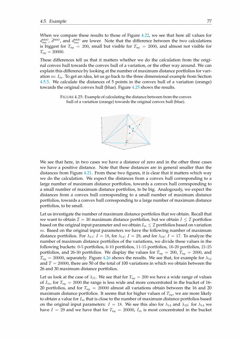
4.5. Example 77
When we compare these results to those of Figure 4.22, we see that here all values fordMDO
min , dMDO, and dMDOmax are lower. Note that the difference between the two calculations
is biggest for Tinp = 200, small but visible for Tinp = 2000, and almost not visible forTinp = 20000.
These differences tell us that it matters whether we do the calculation from the origi-nal convex hull towards the convex hull of a variation, or the other way around. We canexplain this difference by looking at the number of maximum distance portfolios for vari-ation m: Im. To get an idea, let us go back to the three dimensional example from Section4.5.5. We calculate the distances of 5 points in the convex hull of a variation (orange)towards the original convex hull (blue). Figure 4.25 shows the results.
FIGURE 4.25: Example of calculating the distance between from the convexhull of a variation (orange) towards the original convex hull (blue).
We see that here, in two cases we have a distance of zero and in the other three caseswe have a positive distance. Note that these distances are in general smaller than thedistances from Figure 4.21. From these two figures, it is clear that it matters which waywe do the calculation. We expect the distances from a convex hull corresponding to alarge number of maximum distance portfolios, towards a convex hull corresponding toa small number of maximum distance portfolios, to be big. Analogously, we expect thedistances from a convex hull corresponding to a small number of maximum distanceportfolios, towards a convex hull corresponding to a large number of maximum distanceportfolios, to be small.
Let us investigate the number of maximum distance portfolios that we obtain. Recall thatwe want to obtain I = 30 maximum distance portfolios, but we obtain I ≤ I portfoliosbased on the original input parameter and we obtain Im ≤ I portfolios based on variationm. Based on the original input parameters we have the following number of maximumdistance portfolios. For λ11: I = 18, for λ14: I = 29, and for λ19: I = 17. To analyze thenumber of maximum distance portfolios of the variations, we divide these values in thefollowing buckets: 0-5 portfolios, 6-10 portfolios, 11-15 portfolios, 16-20 portfolios, 21-25portfolios, and 26-30 portfolios. We display the values for Tinp = 200, Tinp = 2000, andTinp = 20000, separately. Figure 4.26 shows the results. We see that, for example for λ14and T = 20000, there are 50 of the total of 100 variations in which we obtain between the26 and 30 maximum distance portfolios.
Let us look at the case of λ11. We see that for Tinp = 200 we have a wide range of valuesof Im, for Tinp = 2000 the range is less wide and more concentrated in the bucket of 16-20 portfolios, and for Tinp = 20000 almost all variations obtain between the 16 and 20maximum distance portfolios. It seems that for higher values of Tinp, we are more likelyto obtain a value for Im that is close to the number of maximum distance portfolios basedon the original input parameters: I = 18. We see this also for λ14 and λ19: for λ14 wehave I = 29 and we have that for Tinp = 20000, Im is most concentrated in the bucket
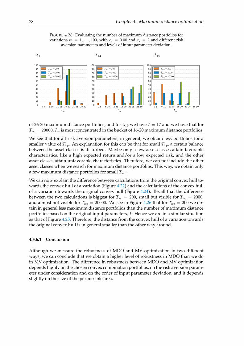
78 Chapter 4. Maximum distance optimization
FIGURE 4.26: Evaluating the number of maximum distance portfolios forvariations m = 1, . . . , 100, with c1 = 0.08 and c2 = 2 and different risk
aversion parameters and levels of input parameter deviation.
0-5 6-10 11-15 16-20 21-25 26-30
Im
0
10
20
30
40
50
60
70
80
90
100
Tinp = 200
Tinp = 2000
Tinp = 20000
0-5 6-10 11-15 16-20 21-25 26-30
Im
0
10
20
30
40
50
60
70
80
90
100
Tinp = 200
Tinp = 2000
Tinp = 20000
0-5 6-10 11-15 16-20 21-25 26-30
Im
0
10
20
30
40
50
60
70
80
90
100
Tinp = 200
Tinp = 2000
Tinp = 20000
λ11 λ14 λ19
of 26-30 maximum distance portfolios, and for λ19 we have I = 17 and we have that forTinp = 20000, Im is most concentrated in the bucket of 16-20 maximum distance portfolios.
We see that for all risk aversion parameters, in general, we obtain less portfolios for asmaller value of Tinp. An explanation for this can be that for small Tinp, a certain balancebetween the asset classes is disturbed. Maybe only a few asset classes attain favorablecharacteristics, like a high expected return and/or a low expected risk, and the otherasset classes attain unfavorable characteristics. Therefore, we can not include the otherasset classes when we search for maximum distance portfolios. This way, we obtain onlya few maximum distance portfolios for small Tinp.
We can now explain the difference between calculations from the original convex hull to-wards the convex hull of a variation (Figure 4.22) and the calculations of the convex hullof a variation towards the original convex hull (Figure 4.24). Recall that the differencebetween the two calculations is biggest for Tinp = 200, small but visible for Tinp = 2000,and almost not visible for Tinp = 20000. We see in Figure 4.26 that for Tinp = 200 we ob-tain in general less maximum distance portfolios than the number of maximum distanceportfolios based on the original input parameters, I . Hence we are in a similar situationas that of Figure 4.25. Therefore, the distance from the convex hull of a variation towardsthe original convex hull is in general smaller than the other way around.
4.5.6.1 Conclusion
Although we measure the robustness of MDO and MV optimization in two differentways, we can conclude that we obtain a higher level of robustness in MDO than we doin MV optimization. The difference in robustness between MDO and MV optimizationdepends highly on the chosen convex combination portfolios, on the risk aversion param-eter under consideration and on the order of input parameter deviation, and it dependsslightly on the size of the permissible area.
79
Chapter 5
Applications
In this chapter, we briefly discuss the applications of the three methods that we considerin this thesis: resampling, shrinkage, and maximum distance optimization. We explainper method the robustness performance, the choices we need to make, and what advan-tages and disadvantages we encounter. Based on these aspects we formulate an adviceto Ortec Finance. We note that there are more methods in the literature than we discussin this thesis, hence the first advice we give is to do further research to other methodsas well. We first discuss the shrinkage method and we continue with resampling andmaximum distance optimization.
5.1 Shrinkage
Shrinkage towards a constant correlation covariance matrix is not useful to Ortec Financefor making portfolios more robust. This method is useful if the number of asset classes islarge compared to the sample size, as we show in Section 3.3.2.
In the application Ortec Finance has in mind, the sample size equals a large number ofscenarios generated in a Monte Carlo simulation and therefore, this method has littleadded value. The method, however, can be of use for Ortec Finance for modeling assetclasses with little historical data.
5.2 Resampling
In Section 2.2.2, we show that resampling produces more robust portfolios. Moreover, re-sampling adds asset classes with near optimal characteristics leading to more diversifiedportfolios.
The robustness effect of resampling follows from the diversification effect. Resamplingresults in a diversified portfolio and if we repeat the same procedure but this time basedon a variation of input parameters, we obtain again a diversified portfolio. And hence,as we showed in Section 2.2.2, the difference between those two portfolios is small.
In resampling, the order of the robustness and diversification effect depends on the num-ber of drawings from a normal distribution, N (µ,Σ). That is, it depends on the parame-ter T . A large value for T results in a small effect and a small value for T results in a largeeffect. However, in the latter case, the effect of robustness and diversification comes ata cost: we give in on the expected portfolio risk and return. Hence, we want to make asmart decision about the value for T but there is no clear guideline to do so. However,
80 Chapter 5. Applications
if we have an idea over how uncertain the input parameters are, this helps us to pick avalue for T .
We note that resampling can produce portfolios such that small shreds of weights aregiven to some asset classes. Investing, for example, less than one percent of the budgetin some asset class is not desirable.
Although not treated in this thesis, the resampling method is applicable to other riskmeasures and other optimization programs. A risk measure that is often used at OrtecFinance is the conditional value at risk (CVaR). For an optimization program that max-imizes the expected return and minimizes the expected CVaR, this method can also behelpful.
A disadvantage, however, is that resampling lacks a theoretical foundation. Intuitively,the method makes sense, but a proper Bayesian framework for example would give themethod a proper theoretical foundation. This issue is often discussed in papers whichcompare resampling with Bayesian optimization, see for example [5].
Lastly, we want to note that there is a possibility on a convex part in the resampled fron-tier. In Section 2.2.3, we show that we probably do not have to worry about this phe-nomenon. We assume a resampling method that only varies the return vector and weprove in Theorem 2.2.2 that the probability of a convex part in the resampled frontierconverges to zero as the number of resamplings goes to infinity. Because we use a vari-ation of the resampling method, this is no guarantee for the original resampling methodbut it is reassuring.
5.2.1 Advice
Resampling has a positive effect on robustness and diversification. Before using resam-pling, one needs to make a well considered decision about the parameter T . This pa-rameter determines a position in a tradeoff between robustness and diversification effectand the loss in expected portfolio risk and return. Resampling is a useful method andwe would recommend to use it. However, we explicitly note that our research is basedon only one example. Before using resampling in practice, we suggest further researchbased on other examples and we suggest to compare resampling to other methods suchas Bayesian optimization or Black Litterman [2] inverse optimization.
5.3 Maximum distance optimization
Maximum distance optimization (MDO) searches for portfolios that are close to optimalin terms of risk and return levels and are far away in terms of allocations. This way, wethoroughly investigate the area closely beneath the efficient frontier.
An advantage of MDO compared to other methods is that it fits well with how a con-sultant of Ortec Finance forms his advice. A consultant combines his expertise with out-comes from the models. In MDO, we obtain a whole range of near optimal portfoliosand any convex combination also results in a portfolio that is near optimal. Therefore, aconsultant can pick a convex combination portfolio that he considers to be best. More-over, the allocations of the near optimal portfolios give a lot of insight. We see whatasset classes are not selected by MV optimization but result however in portfolios thatare almost optimal.
5.3. Maximum distance optimization 81
In Section 4.5.6, we see that MDO results in a range of maximum distance portfolios thatis more robust than a single MV optimal portfolio is.
The diversification effect of MDO depends highly on what convex combination portfoliowe select. Also, both the diversification and the robustness effect of MDO depends on thesize of the area beneath the efficient frontier that we investigate, that is, the permissiblearea. However, the influence of the choice for the permissible area on the robustnessof MDO is limited. For the diversification effect, if we choose a large permissible area,we are likely to obtain portfolios that highly differ in terms of allocations and therefore,we are able to select a diversified convex combination portfolio. If we choose a smallpermissible area, we are likely to obtain portfolios that do not differ a lot in terms ofallocations and therefore, it is likely that we are not able to select a diversified convexcombination portfolio. However, for a small permissible area, we do not necessarilyobtain portfolios with similar allocations, as we discuss in the remarkt below Theorem4.5.1.
A disadvantage of MDO is that the implementation requires a heuristic method. We use aBasin hopping algorithm as heuristic method and we are satisfied about its performance.Good results, however, require a long computation time.
5.3.1 Advice
We advise Ortec Finance to use maximum distance optimization, since the range of max-imum distance portfolios is robust. Morever, MDO fits well with how Ortec Finance usesmodels in combination with their own expert views, to form their advice. MDO givesinsight in what asset classes are not selected by Mean-Variance optimization but resultshowever in portfolios that are only near optimal. Also, MDO, opposed to other methods,gives freedom in selecting a convex combination portfolio that fits well with the expertviews.
We also advise Ortec Finance to extend this method to other risk measures, such as CVaR.The link of Support Vector Machines to calculating the distance towards a convex hull isone that can be used in other optimization programs. Therefore, an extension of MDOto other risk measures is a logical next step. However, we expect that this extension isonly possible if the other risk measure is convex. Otherwise, it is possible that a convexcombination portfolio ends up outside the permissible area.


83
Bibliography
[1] Charalambos D Aliprantis and Kim Border. Infinite dimensional analysis: a hitch-hiker’s guide. Springer Science & Business Media, 2006.
[2] Dimitris Bertsimas, Vishal Gupta, and Ioannis Ch Paschalidis. “Inverse optimiza-tion: A new perspective on the Black-Litterman model”. In: Operations research 60.6(2012), pp. 1389–1403.
[3] Vijay K Chopra and William T Ziemba. “The effect of errors in means, variances,and covariances on optimal portfolio choice”. In: The Kelly Capital Growth InvestmentCriterion: Theory and Practice 3 (2011), p. 249.
[4] docs.scipy.org. https://docs.scipy.org/doc/scipy-0.18.1/reference/generated/scipy.optimize.basinhopping.html. Accessed: 2016-11-21.
[5] Campbell R Harvey, John C Liechty, and Merrill W Liechty. “Bayes vs. resampling:a rematch”. In: (2008).
[6] Olivier Ledoit and Michael Wolf. “Honey, I shrunk the sample covariance matrix”.In: UPF Economics and Business Working Paper 691 (2003).
[7] Olivier Ledoit and Michael Wolf. “Improved estimation of the covariance matrixof stock returns with an application to portfolio selection”. In: Journal of empiricalfinance 10.5 (2003), pp. 603–621.
[8] Harry Markowitz. “Portfolio selection”. In: The journal of finance 7.1 (1952), pp. 77–91.
[9] nobelprize.org. http://www.nobelprize.org/nobel_prizes/economic-sciences/laureates/1990/press.html. Accessed: 2016-01-12.
[10] Bernd Scherer. “Portfolio resampling: Review and critique”. In: Financial AnalystsJournal 58.6 (2002), pp. 98–109.


![Mean-Variance Portfolio Rebalancing with Transaction · PDF fileMean-Variance Portfolio Rebalancing with Transaction Costs ... (Leland [2000] or Donohue and Yip [2003]). ... mean-variance](https://img.pdfslide.net/doc/110x75/5aa9b2147f8b9a81188d1c27/mean-variance-portfolio-rebalancing-with-transaction-portfolio-rebalancing-with.jpg)