Embed Size (px)
Citation preview
i
MEASURE M AND THE POTENTIAL
TRANSFORMATION OF MOBILITY IN
LOS ANGELES
A Research Report from the University of California Institute of Transportation Studies
Prepared for the TransitCenter, New York, New York
PROJECT ID: 2017-01 | DOI:10.7922/G2VT1Q80
4
ABOUT THE UC ITS The University of California Institute of Transportation Studies (UC ITS) is a network of faculty,
research and administrative staff, and students dedicated to advancing the state of the art in
transportation engineering, planning, and policy for the people of California. Established by the
Legislature in 1947, ITS has branches at UC Berkeley, UC Davis, UC Irvine, and UCLA.
ACKNOWLEDGMENTS
This report was funded primarily by TransitCenter, with supplemental funding coming from the
State of California’s SB1 Research Program. I thank Steven Higashide at TransitCenter for
valuable comments and insight throughout the process. I also thank Ana Duran for valuable
research assistance, as well as the numerous UCLA Masters’ students who helped survey transit
riders. LA Metro helpfully provided me with data. Tom Rubin, Dan Chatman and Adam Levine
all gave helpful comments. Seminar participants at Cornell University also improved the
argument, as did Donald Shoup. Miriam Pinksi and Marty Wachs each read an entire draft and
provided valuable feedback. Esther Huang, heroically, proofread the entire thing. All errors are
my own.
DISCLAIMER The contents of this report reflect the views of the author(s), who are responsible for the facts
and the accuracy of the information presented herein. This document is disseminated under
the sponsorship of the State of California in the interest of information exchange. The State of
California assumes no liability for the contents or use thereof. Nor does the content necessarily
reflect the official views or policies of the State of California. This report does not constitute a
standard, specification, or regulation.
5
Measure M and the Potential
Transformation of Mobility in Los Angeles UNIVERSITY OF CALIFORNIA INSTITUTE OF TRANSPORTATION STUDIES
January 2019
Michael Manville, Associate Professor, Department of Urban Planning
UCLA Luskin School of Public Affairs

6
[page intentionally left blank]
7
TABLE OF CONTENTS List of Figures ......................................................................................................................................... 8
List of Tables ........................................................................................................................................... 8
Introduction and Summary ............................................................................................................. 10
II. Transit in America and Los Angeles: Mass Mobility or Redistribution? ............................... 19
III. The Politics of Transit in an Automobile-Oriented Region ...................................................... 26 Activating Identity ...................................................................................................................................................... 26
Indirect Self-Interest .................................................................................................................................................. 27
IV. DATA AND EMPIRICAL APPROACH ................................................................................................... 31
Intercept Survey .......................................................................................................................................................... 34
Results ............................................................................................................................................................... 35
Evaluating the Survey Samples ............................................................................................................................. 35
Support for Measure M ............................................................................................................................................. 38
Intercept Survey Descriptive Statistics .............................................................................................................. 40
Descriptive Analysis of Support for Measure M .................................................................................. 42
How Concerned Are People about Congestion and Transportation? .................................................... 42
What Measure M Brings to Mind .......................................................................................................................... 43
Perceived Beneficiaries of Measure M ............................................................................................................... 45
Associations Between Support for Measure M and Transportation Priorities ................................. 46
Measure M and Attitudes about Travel, and Travel Behavior .................................................................. 49
Regression Analysis of Support for Measure M .................................................................................. 50
Measure M and Support for Transit-Complementary Policies ...................................................... 60
Transit Rider Attitudes ................................................................................................................................ 64
Conclusion ........................................................................................................................................................ 65
References ............................................................................................................................................. 68
8
List of Figures
Figure 1: Trends In Transit Ridership, Rail Ridership, Traffic Congestion And Ballot Success, Los
Angeles County, 1980-2016 .................................................................................................. 13
Figure 2: Responses To Open-Ended Probe About Biggest Issues In LA County .......................... 43
Figure 3: Responses To Open-Ended Probe About Associations With Measure M ..................... 44
Figure 4: Responses To Open-Ended Probe About Beneficiaries Of Measure M ......................... 46
Figure 5: Percent Supporting Freeway Congestion Tolls, November 2016 .................................. 64
List of Tables
Table 1: Socioeconomics of Transit Use in Los Angeles and Six Transit-Heavy US Regions ......... 21
Table 2: Characteristics of LA Metro Riders, LA County Residents, and Transit Riders Overall ... 22
Table 3: Transit Use and Transit Service in Six Transit-Heavy US Regions ................................... 23
Table 4: Income, Density and Parking Availability in Los Angeles and Six Transit-Heavy US
Regions .................................................................................................................................. 25
Table 5: Demographic Characteristics of Online/CATI Survey Sample ......................................... 36
Table 6: Transportation Attributes of Survey Sample .................................................................. 37
Table 7: Summary Knowledge and Support of Measure M .......................................................... 39
Table 8: Summary Statistics, Transit Rider Intercept Survey ........................................................ 41
Table 9: Transportation Priorities for LA County .......................................................................... 47
Table 10: Priorities for Public Transportation ............................................................................... 49
Table 11: Beliefs about Transportation and Transportation Policy .............................................. 50
Table 12: Associations between Support for Measure M and Sociodemographics ..................... 52
Table 13: Associations between Support for Measure M and Partisanship/Ideology ................. 55
Table 14: Associations Between Support for Measure M and Political Knowledge .................... 57
Table 15 : Associations Between Support for Measure M and Beliefs about Transportation ..... 58
Table 16: Opinions about Minimum Parking Requirements ........................................................ 61
Table 17: Opinions about Housing Development ......................................................................... 62
Table 18: Intercept Survey Attitudes and Beliefs ......................................................................... 65

9
10
Introduction and Summary
In the last 20 years, voters in hundreds of localities have chosen to increase their own taxes to
finance billions of dollars of investment in transportation, and especially public transportation.
In November 2016 alone, state and local voters decided on hundreds of such “local option”
transportation taxes. Not all of these taxes financed public transportation. America remains a
highly automobile-oriented country, and some of these initiatives were less about transit and
more about roads. But many were not: at least 50 large initiatives dedicated most of their
revenue to transit (APTA 2016), and by one estimate these 50 measures collectively
represented over $300 billion in transit investment. Over 70 percent of these measures,
representing over $200 billion, were approved (Eno Center for Transportation 2016). Nor was
2016 unique: in most of the last 15 years voters have decided on scores of local option
transportation taxes, the majority of which contained heavy public transit components. Each
year between 60 and 70 percent of these ballots have been approved (Center for
Transportation Excellence, 2006, also Center for Transportation Excellence, nd; Scauzillo 2016).
Even as transit finance has surged, however, transit use has fallen. American transit use has
long been relatively stagnant, and has defied increases in funding and service. While ridership
sees small increases in some years, these are usually counterbalanced by small decreases in
others. From 1970 to 2014, per capita transit service (measured in vehicle revenue miles) rose
46 percent, but per capita ridership fell 6 percent. Even between 2004 and 2013—a rare period
where driving fell while the economy grew—transit use did not rise (Manville et al 2017). After
2013, transit ridership began to fall, first in per capita and then absolute terms. That decline
continues today (Manville et al 2018).
It is possible, of course, that transit use has fallen nationwide but risen in those places where
people turned out to vote for it. Yet this does not appear to be the case. Manville and Cummins
(2014), for example, showed that places with successful transit ballots in the early 2000s had no
discernible mode shifts by 2012, and a cursory examination of places that have approved
ballots since 2012 suggests that little has changed. Almost every urban area has seen ridership
fall in recent years, and places that have approved transit ballot measures do not on balance
seem to be different.1
The juxtaposition of transit’s rising popularity (in at least some places) and its falling ridership
raises the question of why people vote for it. Critics of public transportation have long argued
that transit struggles because political elites force it on voters who don’t want it. Generous
1 There are exceptions to this trend, but they are not, upon closer examination, reassuring. Voters in Phoenix, for example, approved a transit ballot measure in 2015, and in 2017 Phoenix’s transit ridership rose about three percent—making it one of only three urbanized areas where ridership increased. This was a real accomplishment, and Phoenix’s decision to invest in its bus system was probably wise. Yet per capita ridership in Phoenix in 2017 was still lower than it had been in 2015 (19 rides per capita compared to 20) and lower in both years than it had been in 2006 (22). Phoenix, moreover, had also approved a transit ballot measure in 2004; after that victory ridership fell steadily for years (APTA Fact Books, 2008 and 2017).
11
federal incentives, in this view, combined with lobbying by influential insiders, lead elected
officials to supply transit in places where little demand for it exists (e.g. Kotkin and Cox 2017;
Levine et al 1999; Balaker and Kim 2006). Whatever the merits of this critique, it has less
traction when voters explicitly approve higher taxes to fund transit. Transit ballots are thus a
small rebuke to the idea that transit supply is the result of elite imposition. The government, in
these cases, seems to be giving voters what they want. Voters just seem to want transit for
reasons other than riding it.
What might those reasons be? The answer to this question is obviously of interest to transit
advocates. Knowing what makes voters turn out to support transit can help advocates win
more elections and finance more service. But the answer may also hold clues for transit’s
longer-term trajectory. If political support for transit finance is largely divorced from any desire
to ride transit—if it is rooted in partisanship, or a desire to help low-income people who already
use transit, or a belief that better transit will make driving easier—then even large ballot box
victories may not imply changes in mobility or travel behavior.
This report examines the motivations behind transit ballots by analyzing Measure M, a large
transportation sales tax that voters in Los Angeles County approved on Election Day 2016. The
Measure was advanced by LA Metro, the Los Angeles region’s largest transportation agency,
and won with 71.5 percent of the vote, easily exceeding the difficult two-thirds threshold that
California requires for new taxes or tax increases. Formally titled the “Los Angeles County
Traffic Improvement Plan,” Measure M permanently raised the county sales tax by ½ cent and
also made an earlier, temporary transportation sales tax increase permanent. All told,
proponents estimate that Measure M will generate $860 million a year, or more than $120
billion over 40 years. The measure is multimodal: in addition to transit, it will fund road
projects, as well as bicycle and pedestrian infrastructure. But fully 65 percent of its funding is
for transit, and transit dominated both the coverage and rhetoric of its campaign.
Los Angeles is just one region, and Measure M is just one ballot measure. So, there are limits to
the generalizability of this report’s findings. Yet Measure M remains a useful case study, for
three reasons. First, it is a large and prominent transportation measure, with most of its
revenue and rhetoric focused on transit. Second, Measure M is not the first transit-focused
local option tax that LA County has approved. Even before Measure M, over 40 percent of LA
Metro’s annual revenue came from local sales taxes—the result of three additional local option
transportation sales taxes, approved in 1980, 1990 and 2008, that each raised the sales tax by ½
cent. All of these measures devoted at least a plurality of its revenue to transit (especially rail)
and each was accompanied by political rhetoric about reducing congestion and pollution, and
shifting LA away from its primarily automobile-focused patterns of moving around.
Because Los Angeles is not new to ballot box transportation finance, using Measure M as a case
study helps control for at least one potential confounding factor—transportation transitions
take time. Expecting residents to immediately shift from automobiles to trains and buses is in
many cases simply not realistic, meaning that short-run examinations of places where transit
12
ballots passed is unlikely to be informative. In such places changes may occur slowly as systems
are built, people become accustomed to using transit, and so on.
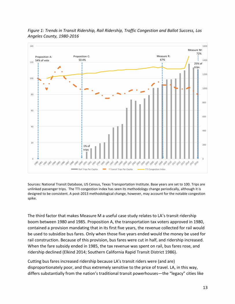
Los Angeles, in contrast, has had ample time to begin this transition. Figure 1 shows that while
the region’s political victories have led to dramatic changes in transit service, they have been
less successful in delivering the intended outcomes of more ridership and less congestion.2 The
text at the top of the graph displays the share of the vote won by each of LA’s four successful
transportation ballots; in recent years transit finance has become more popular. Where 1980’s
Propositions A and 1990’s Proposition C won fairly narrow victories (54 percent and 50.4
percent of the vote, respectively), Measures R and M, in 2008 and 2016, both captured over
two-thirds of the vote.
The figure’s vertical bars, which show per capita rail ridership, suggest that the revenue from
these ballot measures has fueled an undeniable transformation in LA’s transit system. In 1980
Los Angeles had no heavy or light rail. By 2016 it had over 110 miles of rail, with more under
construction. In 1991, when the county’s first rail line opened, rail carried 1 percent of LA
Metro’s trips. Over the next 25 years, rail ridership grew over 1,200 percent (from an
admittedly small base) and by 2016 rail accounted for 25 percent of Metro’s trips.
But rail’s expansion was not accompanied by falling congestion, and was accompanied by falling
ridership. The solid line that trends upward across the top of the graph shows the Texas
Transportation Institute’s Travel Time Index (TTI) for Los Angeles. Congestion delay was over
ten percent higher in the 2010s than it was in the early 1980s. The TTI index is an admittedly
imperfect metric of congestion, but by most metrics—average delay, reliability, and so on—LA’s
congestion has worsened over time.3 Finally, the graph’s heavy dashed line, which represents
overall ridership per capita, shows that the county’s transit use has been falling. After surging
from 1980 to 1985 (a phenomenon I will explain below) LA’s ridership began to fall and never
recovered. By 2016, Metro’s per capita ridership was 20 percent lower than its 1980 level, and
40 percent below its 1985 peak. In sum, LA voters have consistently voted for transit and
consistently not used it.
2 For most variables 1980 is set to 100, except rail ridership (which did not start until 1991) and the congestion index (which did not begin until 1982). 3 The TTI measures the ratio of peak driving time to off-peak driving time: a TTI of 1.4, for example, suggests that it takes 40 percent longer to make a trip at peak hours than off-peak. The TTI attracts a good deal of criticism, and much of that criticism is justified. One relevant issue is that the methodology used to build the TTI has changed over time; Figure 1 shows a dramatic spike in the TTI after 2012, and this probably represents a change in measurement, rather than a huge leap in congestion. The most persuasive criticisms of the TTI, however, are not that it inaccurately measures road delay, but that a) people inappropriately use it as a metric of mobility, and b) people use it as a foundation for building inaccurate estimates of congestion’s total costs (Cortright 2010; Littman 2014). I believe both these criticisms are valid, but they have little bearing on my use of the index in Figure 1. Rail transit was supposed to reduce road delay in Los Angeles, and the index is a reasonable (although, again, imperfect) metric of road delay.
13
Figure 1: Trends in Transit Ridership, Rail Ridership, Traffic Congestion and Ballot Success, Los Angeles County, 1980-2016
Sources: National Transit Database, US Census, Texas Transportation Institute. Base years are set to 100. Trips are unlinked passenger trips. The TTI congestion index has seen its methodology change periodically, although it is designed to be consistent. A post-2013 methodological change, however, may account for the notable congestion spike.
The third factor that makes Measure M a useful case study relates to LA’s transit ridership
boom between 1980 and 1985. Proposition A, the transportation tax voters approved in 1980,
contained a provision mandating that in its first five years, the revenue collected for rail would
be used to subsidize bus fares. Only when those five years ended would the money be used for
rail construction. Because of this provision, bus fares were cut in half, and ridership increased.
When the fare subsidy ended in 1985, the tax revenue was spent on rail, bus fares rose, and
ridership declined (Elkind 2014; Southern California Rapid Transit District 1986).
Cutting bus fares increased ridership because LA’s transit riders were (and are)
disproportionately poor, and thus extremely sensitive to the price of travel. LA, in this way,
differs substantially from the nation’s traditional transit powerhouses—the “legacy” cities like
0
200
400
600
800
1000
1200
1400
1600
0
20
40
60
80
100
120
140
Rail Trips Per Capita Transit Trips Per Capita TTI Congestion Index
Proposition A: 54% of vote
Proposition C:50.4%
Measure R:67%
Measure M: 72%
1% of trips
25% of trips
14
New York, San Francisco and Boston that grew up around public transportation. In these places,
older built environments with narrow streets and scarce parking give transit relative
advantages over driving, leading middle class and even affluent people use public
transportation regularly.
Los Angeles, despite once boasting a vast public transportation network (Wachs 1996), is not a
legacy transit city. In absolute terms, Los Angeles has large transit ridership, one that exceeds
the ridership in many of the smaller legacy regions. But its built environment and
transportation culture are oriented resolutely around the automobile, and as a result transit in
Los Angeles is used primarily by low-income, often foreign born, people who lack access to
private cars. Public transportation in Los Angeles is more a social service than it is a widely-
shared form of mobility. The success of 1980’s fare reduction should be understood in this
context. Lower fares probably increased LA’s ridership more by allowing people who already
used transit to use it more frequently, rather than by encouraging people who once drove to
begin taking transit instead. Cutting fares in 1980 created more ridership, but not necessarily
many new riders. There is at least some reason to think the cutting fares today would have a
similar result.
Measure M’s implicit goal, however, is different. Measure M is not designed to offer a more
generous transportation social safety net, nor to convince current riders to ride more often.
The goal instead was to transition LA from a social service model of transit to one where transit
is a more universal way of moving around, a model more closely resembling the transit systems
of the legacy northern cities. Measure M’s campaign rhetoric frequently invoked the idea of
less congestion, and a Los Angeles where more people would have more choices about how
they move around. In the run-up to the election, Metro’s CEO regularly said that one of his
goals was to make 25 percent of LA County residents regular transit riders (Nelson 2016).
The ambition of this goal should not be understated. Los Angeles is trying to accomplish,
through electoral politics and public policy, what cities like Boston and New York accomplished
largely through the accident of history. America’s legacy transit cities did not divorce the
automobile. They were married to transit from the start. The tension that LA must navigate, in
trying to maintain its social service while also attracting drivers, is felt less acutely in legacy
cities.
Crucially, LA’s challenge is the challenge that most American cities will face, should they also
attempt to move away from driving and toward transit. Just as it is in LA, public transportation
in most American cities is a social service, so Los Angeles represents a potential future for these
places—a bellwether for the broader effort to remake America cities in a less car-centric image.
LA may offer few lessons for how a transportation tax would play out in San Francisco or
Philadelphia, but almost certainly offers insight into the political prospects for public
transportation in Atlanta or Nashville or Houston.
15
Examining Measure M requires understanding it as a transportation proposal, a tax proposal,
and a political problem—since it was all these things. My analysis of the measure draws on
some publicly-available government data and a brief review of the election’s campaign
materials. I build most of the analysis, however, on two surveys that I wrote and supervised: a
probability survey of LA County adults carried out immediately after the election, and a survey
of transit riders conducted a few months later. I use these surveys, combined with the other
data, to draw some broad conclusions about why Measure M passed, and what that might
mean for transit use in LA County.
My findings, in brief, are as follows:
Support for Measure M fell heavily along ideological and especially partisan lines; liberals and
Democrats supported the measure, while conservatives and Republicans did not. Self-
identified liberals and especially self-identified Democrats were much more likely to support
Measure M than were conservatives, Republicans, or people who indicated a preference for
small government. This relationship was robust: Democrats supported Measure M more than
Republicans, and “strong Democrats” supported it more than Democrats overall. These finding
accord with some newer work in political science (Niall 2017) suggesting that transportation
issues have become increasingly partisan, and more likely to be decided by party identity rather
than personal relevance.
Support for Measure M was support for public transportation: Measure M, like many local
option transportation taxes, was multimodal. Most of the revenue it raised would go towards
transit, but its spending plan included considerable funding for roads and freeways. The
presence of automobile improvements in local option transportation taxes raises a potential
explanation for why their approval is not accompanied by rising transit ridership: transportation
taxes might succeed despite, rather than because of, their transit components. In short, voters
approve transit spending, but are actually motivated by road spending (e.g. Manville and
Cummins 2014). This explanation, however, does not appear to hold with Measure M. Support
for Measure M was strongly associated with positive attitudes toward public transportation.
Attitudes toward transit, in fact, are one of the major differences between supporters and
opponents. This conclusion does not mean Measure M’s road funding was politically
unnecessary. Given the high voter threshold Measure M needed to clear, road funding may well
have delivered some essential votes. But Measure M’s support was very much driven by
enthusiasm for transit.
Concerns about traffic congestion did not, by themselves, predict support for Measure M. But
people concerned about congestion who also felt positively about transit were very likely to
support the Measure. Measure M’s campaign heavily emphasized the goal of alleviating LA’s
notorious traffic congestion. My survey results suggest that this message was effective, but not
simply because voters dislike congestion. Virtually everyone in LA County appears to dislike
congestion, so concerns about congestion, by themselves, had little association with support
for Measure M. Indeed, the people most concerned about traffic congestion—people who
16
volunteered, unprompted, that congestion was one of LA County’s two biggest problems—
were no more likely than others to support Measure M. What set Measure M supporters apart
was a concern about congestion combined with positive ideas about transit. People who had
positive beliefs about transit were more likely to associate Measure M with congestion, and
much more likely to support the measure. This finding accords with broader findings from
political science: to succeed, political entrepreneurs must both define a problem and frame
their preferred policy as a solution to that problem. The latter is harder than the former, but
when people concerned about congestion become convinced that transit can help reduce it,
they vote for transit.
Both supporters and opponents of Measure M want public transportation to reduce
congestion and improve the environment. Few survey respondents see transit’s current role—
helping provide mobility to low-income people—as a high priority. Almost 70 percent of
Measure M supporters, and over 75 percent of opponents, see transit’s top priority as either
reducing congestion or improving the environment. Only 20 percent of supporters and 16
percent of opponents view transit’s top priority to be improving mobility for low-income
people.
Demographically, the average Measure M supporter does not resemble a likely transit rider.
Riding transit in Los Angeles is largely a function of socioeconomic status, and particularly of
access to private vehicles (Manville et al 2018). Support for Measure M, in contrast, is
associated less with socioeconomic status and more with particular beliefs and attitudes. Most
Measure M supporters, like most county residents, live firmly auto-oriented lifestyles. They
own automobiles and have free parking at home and work. Many have high incomes. All of
these attributes predict driving. Measure M supporters are more likely than opponents to say
that they would like to drive less, but in regression analysis the association between this
attitude and support for Measure M is inconsistent. In contrast, the differences between
Measure M supporters and opponents become much larger, and statistically significant, when
they express beliefs about the social, as opposed to the personal, value of transit. Measure M’s
support does not appear to stem from any widespread desire to personally ride transit more,
but instead from a belief that if the region has more transit, some people will ride it, and that as
a result progress will be made against various social problems.
The public’s strong support for Measure M is counterbalanced by deep ambivalence about
complementary policies—building more housing, reforming parking, or tolling freeways—that
would make the measure effective. Financing transit is a necessary but not sufficient condition
for robust transit ridership. The American cities where transit captures a substantial share of
travel combine transit investment with policies that make riding transit easier and driving
private vehicles harder. In these places, central city housing and population densities are high,
streets are narrow, blocks are short, and parking is scarce and expensive. None of these
characteristics describe Los Angeles. For a large city, LA’s central densities are relatively low, its
roads are wide, and parking is abundant. These factors, which arise at least in part from
17
deliberate policy decisions, not only make driving easier but also hobble transit’s effectiveness.
Without changes in these policies, even a well-financed transit system is unlikely to lure many
riders. But public support for such changes—expressed in beliefs about the costs and benefits
of more housing development or parking reform—is far lower than support for Measure M.
A substantial minority of LA’s current public transportation riders would prefer to drive.
Metro’s rider surveys consistently show that upwards of 70 percent of riders do not have a
vehicle to make their transit trip; my own survey of riders shows the same. My results,
moreover, suggest that over 40 percent of those vehicle-free riders would not ride transit (or
would ride less) if they had access to cars. Thus, almost 30 percent of LA’s current transit riders
would rather not be on transit, or be on it less.
How should we interpret these results? For transit advocates, they clearly suggest a path
toward political success in car-oriented cities. The dominant transportation concern in such
places is often traffic congestion. Most voters are drivers, and the typical problem that drivers
encounter is congestion. Tapping into frustration with congestion (and to a lesser extent into
concerns about the environment), and depicting public transit as a solution, could encourage
people who have little personal experience with transit to support it. The results also suggest
that transit advocates should be mindful of trends in local partisanship. To the extent transit is
increasingly associated with Democratic identity, advocates can time transit ballots around
other elections that promise strong Democratic turnout.
More broadly, however, the results might give advocates some pause. If support for transit
finance is fueled by concern about congestion and partisan identity, then it may not be
motivated by a desire to use transit. If this is the case, then the political project of securing
transit funding may be orthogonal to, or even at odds with, the policy project of encouraging
transit ridership. Victory in a transit election is both a political end and a policy means: an
electoral win is the final step in the political process, but an intermediate step in the
transportation policy process, where the desired outcome is (presumably) a successful transit
system. If the factors that determine the former do not necessarily determine the latter, then
we cannot extrapolate from victory at the polls to expectations about changed mobility.
For example, if people vote for transit largely out of allegiance to Democratic priorities, there is
little reason to think the electoral outcome will translate into different travel behavior. And if
people vote for transit because they want less congestion, the source of transit’s electoral
support might actually inhibit changes in travel behavior. People who vote for transit because
they believe it reduces congestion are often voting for transit because they want driving to be
easier. But transit works best in places where driving is harder. Transit, again, thrives in dense
environments where walking is easy and parking is difficult. These environments help transit by
making transit itself more effective (more people can more easily access stops) but also
18
because they raise the price of driving, in time or stress or money, by taking some space away
from vehicles.4
Selling transit as a way to reduce congestion, in other words, is a strategy with a contradiction
embedded in it. Voters who support transit because they want their driving to be easier are
unlikely to support policies that will make transit effective, because those policies will
intrinsically make driving harder. A broad agreement about financing transit will mask
underlying disagreement about transit’s purpose, and about how the city should allocate space
across modes. If an electorate agrees about financing transit but remains divided over policies
that would support it, then transit service can increase even as transit effectiveness remains
low. In these circumstances the typical resident is unlikely to be drawn out of their car and onto
transit. Transit will continue to be a social service, and because its service quality and
convenience will remain low relative to driving, many of the low-income people who ride
transit will leave it when they are able. Transit riders will aspire to drive, and drivers will not
aspire to ride transit. In many ways, this is the pattern we have seen play out in Los Angeles.
The remainder of the report proceeds as follows. The next section highlights the profound
differences between Los Angeles and the America’s legacy transit cities. I then review the
history of transit ballots in LA, and summarize the Measure M campaign. Section IV introduces
my survey data and methods, and the fifth section presents the results. In the final section I
discuss the implications of these findings for transit policy in LA and cities like it.
4 I discuss this point further throughout the report, but for now a caveat is in order. In some ways bus transit might do better in places where driving is easier, since many buses share road space with private vehicles, and if private vehicles are moving unimpeded then so too are buses. At the same time, if private vehicles are moving unimpeded then most people (if they have cars) will have little incentive to be on a bus. In congested areas, bus transit is more effective when driving is more difficult relative to buses (the buses have their own lanes) or more expensive (roads are congestion-charged and buses are exempt).
19
II. Transit in America and Los Angeles: Mass Mobility or Redistribution?
Most people in most parts of America do not use public transportation. The average American
took 36 transit trips in 2016, but the median and modal American took zero (Manville et al
2018). This divergence between the mean and mode arises because the typical American does
not ride transit at all, while a small share of people ride it intensively. America’s low overall use
of transit owes in part to transit’s complete absence in some places: about 20 percent of
Americans don’t live near public transportation. Yet even in regions with transit, most people
don’t ride. Nor do most Americans believe transit should expand. In most years a majority of
Americans, when asked, say they do not support more spending on public transportation.5
While transit often looms large for people concerned about transportation policy, it plays little
role in most people’s lives. The United States is built for driving, and the vast majority of
personal travel occurs by private car.
Given the car’s dominance, American transit ridership is concentrated among people for whom
access to a private car is difficult. This difficulty can arise from some combination of two
reasons: because driving itself is expensive (an attribute of a place), or because incomes are low
(an attribute of people). Driving is expensive in only a handful of places: dense central cities
with narrow streets, heavy congestion, and little parking. In such places, even affluent people
ride transit, because the cost of regular car use (in money, time or stress) is prohibitive. Outside
these areas, transit is demographically concentrated among people with low-incomes, or
people who have medical or legal constraints that prevent them from driving. We can thus
draw a distinction between a mass market mobility model of transit—places where transit is a
relatively convenient way to move around—and a social service model—places where transit is
a safety net for people locked out of the dominant form of mobility (Glaeser et al 2008; Taylor
and Morris 2014).
In the US, the social service model describes most transit systems, while the mobility model
accounts for most transit riders—because, again, transit ridership is heavily concentrated in a
few places. Most systems are sparsely-used, and used mostly by poorer people, while a handful
are heavily used, and used by people of all socioeconomic strata. The National Transit
Database tracks transit service in 531 urbanized areas. In 2016, just seven of these areas—New
York, Los Angeles, Washington DC, Philadelphia, San Francisco, Boston and Chicago—accounted
5 The General Social Survey asks a representative sample of Americans this question every two years. Since 2000,
the share of respondents saying “too little” (i.e., they want to spend more on transit), has averaged 36 percent. This proportion has sometimes climbed to 45 percent, but never exceeded 50 percent. The share of people who prioritize transit over roads—who support more transit spending but do not support more highway spending—averages closer to 20 percent. The American Public Transportation Association (APTA) has occasionally commissioned surveys showing that far higher shares of Americans (upwards of 70 percent) want more transit spending, but the GSS is a high-response-rate gold-standard survey, and its results are likely more accurate. Other surveys, some reviewed in Manville and Cummins (2014) also suggest that national support for increased transit spending is well below 50 percent.
20
for 46 percent of transit service,6 and 69 percent of transit ridership, despite holding just 25
percent of the population. New York alone, which is 8 percent of the population, accounts for
over 40 percent of all US ridership and 20 percent of service.7 Even these figures understate
transit’s geographic concentration, since the ridership occurs largely in the central cities of
these urban areas.
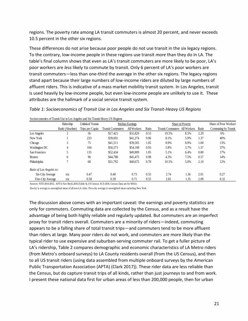
Among these seven transit-heavy regions, Los Angeles stands out. Unlike the other regions, LA
is not a legacy transit city, and operates with a social service model of transit, as Tables 1 and 2
illustrate. Table 1 shows ridership data for each of these seven regions, as well as data on the
median earnings and poverty status of commuters. The table’s next-to-last row compares LA to
the unweighted average of the other six cities. Because New York is such an outlier, the final
row compares LA to the unweighted average of the five regions other than New York.
The table’s first column shows each region’s rank in absolute ridership. In general, bigger places
contribute more to US transit ridership: New York is first, LA second, and so on. The second
column, however, shows per capita ridership, and here we see that New York is truly a region
unto itself. With 233 trips per capita, New York far outdistances the next-highest region, San
Francisco (135 trips). LA, meanwhile, plunges from second-place in absolute terms to dead last
in per capita terms, at only 56 trips per capita. The next-smallest per capita ridership is found in
Philadelphia, a smaller region whose central city has struggled for decades with population loss,
but whose ridership remains 21 percent higher than LA’s.
The table’s remaining columns put LA’s low per capita ridership into context. LA is a large
source of total US transit ridership, but not because a large share of Angelinos use transit. The
region’s contribution instead stems from LA simply having many people, and particularly many
poor people. We can see this both by comparing LA’s transit commutes to commuters in the
other regions, and by comparing LA’s transit commuters to LA’s workers overall. Transit
commuters in Los Angeles have lower earnings and higher poverty rates than transit
commuters in the other regions, and the earnings gap between LA’s transit commuters and the
LA workforce overall is much larger than the gap in the other regions. Transit commuters in Los
Angeles have less than half the median earnings of transit commuters in the other six regions,
even though earnings for workers in overall are closer to three-quarters the earnings of
workers in the other regions. The average LA worker, meanwhile, has twice the median
earnings of the average LA transit commuter (almost $33,000 compared to $17,400). In the
other six regions, in contrast, transit commuters’ median earnings are much closer to, and
sometimes exceed, the median earnings of workers overall (e.g., transit commuters in Chicago
have median earnings 5 percent higher than the larger Chicago workforce). Similarly, LA’s
transit commuters are more than twice as likely to be poor as LA workers overall (19.5 percent
to 8.5 percent), and almost three times as likely to be poor as transit commuters in the other
6 Measured in vehicle revenue miles. 7 Calculated from National Transit Database’s 2016 UZA Allocation Tables.
21
regions. The poverty rate among LA transit commuters is almost 20 percent, and never exceeds
10.5 percent in the other six regions.
These differences do not arise because poor people do not use transit in the six legacy regions.
To the contrary, low-income people in these regions use transit more than they do in LA. The
table’s final column shows that even as LA’s transit commuters are more likely to be poor, LA’s
poor workers are less likely to commute by transit. Only 6 percent of LA’s poor workers are
transit commuters—less than one-third the average in the other six regions. The legacy regions
stand apart because their large numbers of low-income riders are diluted by large numbers of
affluent riders. This is indicative of a mass market mobility transit system. In Los Angeles, transit
is used heavily by low-income people, but even low-income people are unlikely to use it. These
attributes are the hallmark of a social service transit system.
Table 1: Socioeconomics of Transit Use in Los Angeles and Six Transit-Heavy US Regions
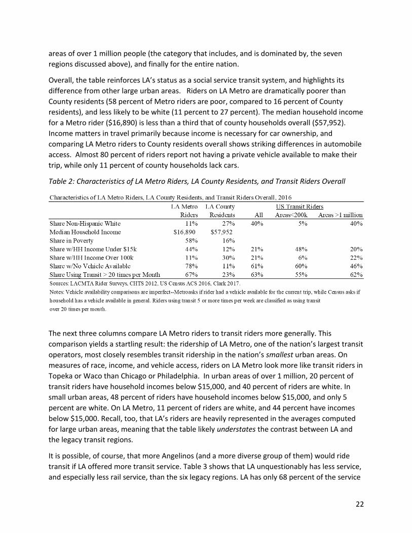
The discussion above comes with an important caveat: the earnings and poverty statistics are
only for commuters. Commuting data are collected by the Census, and as a result have the
advantage of being both highly reliable and regularly updated. But commuters are an imperfect
proxy for transit riders overall. Commuters are a minority of riders—indeed, commuting
appears to be a falling share of total transit trips—and commuters tend to be more affluent
than riders at large. Many poor riders do not work, and commuters are more likely than the
typical rider to use expensive and suburban-serving commuter rail. To get a fuller picture of
LA’s ridership, Table 2 compares demographic and economic characteristics of LA Metro riders
(from Metro’s onboard surveys) to LA County residents overall (from the US Census), and then
to all US transit riders (using data assembled from multiple onboard surveys by the American
Public Transportation Association (APTA) (Clark 2017)). These rider data are less reliable than
the Census, but do capture transit trips of all kinds, rather than just journeys to and from work.
I present these national data first for urban areas of less than 200,000 people, then for urban
Socioeconomics of Transit Use in Los Angeles and Six Transit-Heavy US Regions
Ridership Unlinked Transit Share of Poor Workers
Rank (Absolute) Trips per Capita Transit Commuters All Workers Ratio Transit Commuters All Workers Ratio Commuting by Transit
Los Angeles 2 56 $17,421 $32,820 0.53 19.5% 8.5% 2.29 6%
New York 1 233 $39,691 $41,274 0.96 8.1% 5.9% 1.37 40%
Chicago 3 75 $41,511 $39,505 1.05 8.9% 8.9% 1.00 13%
Washington DC 4 104 $50,273 $54,108 0.93 5.8% 3.7% 1.57 37%
San Francisco 5 135 $52,434 $49,809 1.05 5.1% 6.4% 0.80 17%
Boston 6 96 $44,788 $45,475 0.98 4.3% 7.5% 0.57 14%
Philadelphia 7 68 $31,792 $40,675 0.78 10.5% 5.0% 2.10 12%
Ratio of Los Angeles to:
Six-City Average n/a 0.47 0.40 0.73 0.55 2.74 1.36 2.01 0.27
Five-City Average n/a 0.58 0.39 0.71 0.55 2.82 1.35 2.09 0.32
Sources: NTD 2014-2015, APTA Fact Book 2016 (Table 4), US Census ACS 2016. Census Data are for MSAs
Six-city is average is unewighted mean of all non-LA cities. Five-city average is unweighted mean excluding New York.
Median Earnings Share in Poverty
22
areas of over 1 million people (the category that includes, and is dominated by, the seven
regions discussed above), and finally for the entire nation.
Overall, the table reinforces LA’s status as a social service transit system, and highlights its
difference from other large urban areas. Riders on LA Metro are dramatically poorer than
County residents (58 percent of Metro riders are poor, compared to 16 percent of County
residents), and less likely to be white (11 percent to 27 percent). The median household income
for a Metro rider ($16,890) is less than a third that of county households overall ($57,952).
Income matters in travel primarily because income is necessary for car ownership, and
comparing LA Metro riders to County residents overall shows striking differences in automobile
access. Almost 80 percent of riders report not having a private vehicle available to make their
trip, while only 11 percent of county households lack cars.
Table 2: Characteristics of LA Metro Riders, LA County Residents, and Transit Riders Overall
The next three columns compare LA Metro riders to transit riders more generally. This
comparison yields a startling result: the ridership of LA Metro, one of the nation’s largest transit
operators, most closely resembles transit ridership in the nation’s smallest urban areas. On
measures of race, income, and vehicle access, riders on LA Metro look more like transit riders in
Topeka or Waco than Chicago or Philadelphia. In urban areas of over 1 million, 20 percent of
transit riders have household incomes below $15,000, and 40 percent of riders are white. In
small urban areas, 48 percent of riders have household incomes below $15,000, and only 5
percent are white. On LA Metro, 11 percent of riders are white, and 44 percent have incomes
below $15,000. Recall, too, that LA’s riders are heavily represented in the averages computed
for large urban areas, meaning that the table likely understates the contrast between LA and
the legacy transit regions.
It is possible, of course, that more Angelinos (and a more diverse group of them) would ride
transit if LA offered more transit service. Table 3 shows that LA unquestionably has less service,
and especially less rail service, than the six legacy regions. LA has only 68 percent of the service
23
(in vehicle revenue hours per capita) of the other six regions (with New York excluded, it has
three quarters of the service), and has only 13 percent of the per capita rail service.
At the same time, the broader transit literature suggests that more service does not
automatically yield more ridership. Service levels are both a cause and a consequence of transit
use. Places with more service will attract more riders, but places that attract more riders also
provide more service. New York has many riders because it has an extensive rail system, but
that system exists in part because many people want to ride. Taylor et al (2009), in a large study
of hundreds of urban areas that controlled for this reverse causation, found that service levels
explained only about 25 percent of the total variance in ridership (i.e., the difference between
the urban areas with the most and least ridership). Service differences likely explain much less
of the ridership gap between LA and the other large regions.
Table 3: Transit Use and Transit Service in Six Transit-Heavy US Regions
What then would explain LA’s different performance? Taylor et al (2009) determined that most
inter-regional differences in transit ridership resulted from factors—usually beyond the control
of transit operators—that influenced the relative prices of using transit and driving. Vehicle
ownership is among the most important of these factors (Manville et al 2018) and vehicle
ownership is itself often a function of not just income but also of density and parking
availability. Cars are expensive to own, use and store. Higher income can help households buy
and maintain cars, while areas with more space, and especially more space devoted to parking,
can make it easier to store and operate them.
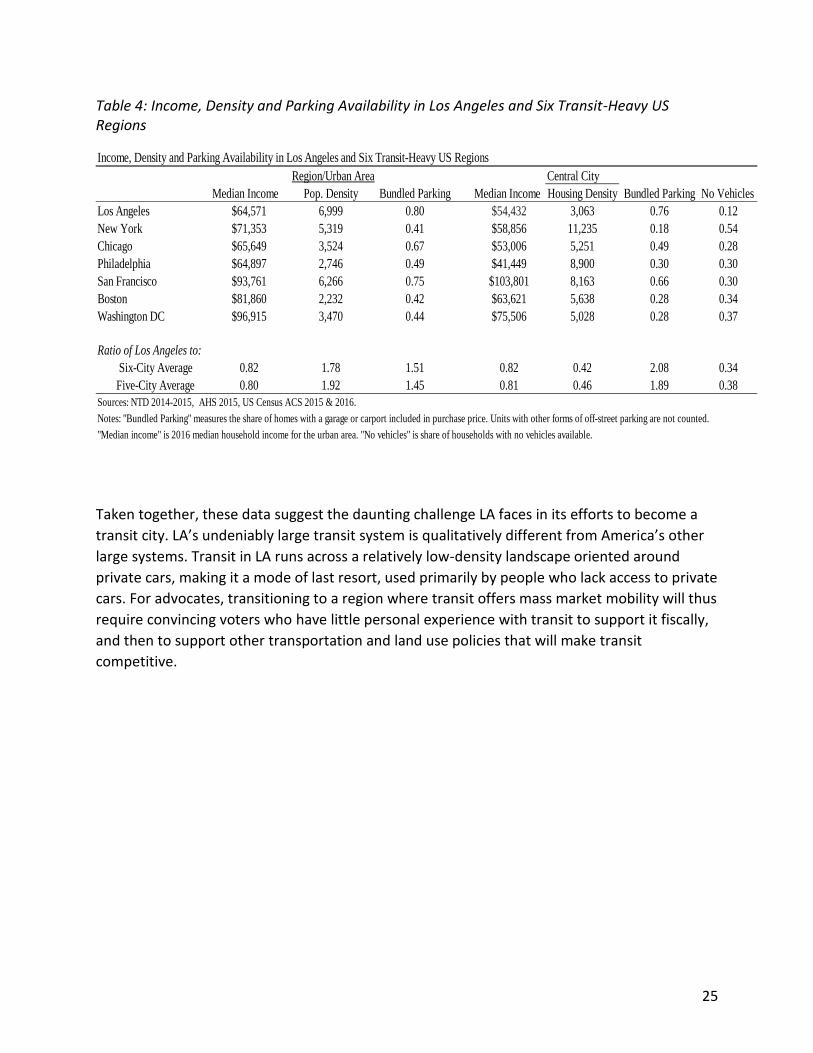
Table 4 compares LA to the six legacy regions on measures of income, density, parking
availability, and vehicle ownership. The table’s first column shows that compared to the other
Transit Use and Transit Service in Los Angeles and Six Transit-Heavy US Regions
Unlinked Transit Vehicle Revenue Rail VRH
Trips per Capita Hours per Capita per Capita
Los Angeles 56 1.5 0.08
New York 233 3.0 1.09
Chicago 75 1.8 0.46
Philadelphia 68 1.4 0.19
San Francisco 135 2.5 0.74
Boston 96 1.8 0.49
Washington DC 104 2.7 0.75
Ratio of Los Angeles to:
Six-City Average 0.47 0.68 0.13
Five-City Average 0.58 0.73 0.16
Sources: NTD 2014-2015, AHS 2015, US Census ACS 2015
24
regions, median income in Los Angeles is rather low; it is about 80 percent of the average of the
other regions, and only Philadelphia’s income is lower. The second column shows that the LA
region is quite dense; it is in fact denser than any of the legacy regions. Superficially these
factors present a puzzle. LA’s combination of lower income and higher density should, all else
equal, suggest higher transit use.
The rest of the table resolves the puzzle. LA’s high average density is deceptive, in that it
conceals both the absence of a very dense core and the automobile-orientation of the
landscape. Unlike many legacy regions, whose high densities are driven by extremely dense
central areas, LA is dense primarily because it has dense suburbs (Manville et al 2013; Manville
and Shoup 2005; Eidlin 2010). As a result, LA has a landscape that, despite its density, demands
and caters to driving. The table’s third column shows the share of housing units in each region
that come with a garage or carport in the rent or purchase price. In LA this proportion is 80
percent, over 50 percent larger than the average of the six other regions, and twice the
proportions in Boston and New York.
The table’s remaining columns compare each region’s central city. Central cities tend to be
where most regional transit use occurs, because they have higher densities, less parking, and
less vehicle ownership. Once again, we see that compared to the other regions, income is lower
in LA. But this lower income, which should tend toward lower levels of driving, is
counterbalanced by a driving-oriented built environment. The central cities of the legacy
regions are densely-built places with little parking; LA City, in contrast, has a housing density
less than half that of the legacy central cities. In the legacy central cities, the share of housing
units that include parking falls off dramatically, but in LA the share of housing units that include
a garage or carport is essentially the same as the proportion for the region as a whole. When
parking is bundled into housing in central cities vehicle ownership rises (Manville 2017), and
indeed carlessness in LA City is rare, despite the city’s relatively low income. Only 12 percent of
LA City households have no vehicle, which is less than one third the average in other cities.
Households in San Francisco, where the median income is over $103,000, are more than twice
as likely to be carless as households in LA, where the median household income is $54,400. LA’s
built environment lowers the price of driving, and this lower price more than compensates for
its residents’ lower incomes.
25
Table 4: Income, Density and Parking Availability in Los Angeles and Six Transit-Heavy US Regions
Taken together, these data suggest the daunting challenge LA faces in its efforts to become a
transit city. LA’s undeniably large transit system is qualitatively different from America’s other
large systems. Transit in LA runs across a relatively low-density landscape oriented around
private cars, making it a mode of last resort, used primarily by people who lack access to private
cars. For advocates, transitioning to a region where transit offers mass market mobility will thus
require convincing voters who have little personal experience with transit to support it fiscally,
and then to support other transportation and land use policies that will make transit
competitive.
Income, Density and Parking Availability in Los Angeles and Six Transit-Heavy US Regions
Central City
Median Income Pop. Density Bundled Parking Median Income Housing Density Bundled Parking No Vehicles
Los Angeles $64,571 6,999 0.80 $54,432 3,063 0.76 0.12
New York $71,353 5,319 0.41 $58,856 11,235 0.18 0.54
Chicago $65,649 3,524 0.67 $53,006 5,251 0.49 0.28
Philadelphia $64,897 2,746 0.49 $41,449 8,900 0.30 0.30
San Francisco $93,761 6,266 0.75 $103,801 8,163 0.66 0.30
Boston $81,860 2,232 0.42 $63,621 5,638 0.28 0.34
Washington DC $96,915 3,470 0.44 $75,506 5,028 0.28 0.37
Ratio of Los Angeles to:
Six-City Average 0.82 1.78 1.51 0.82 0.42 2.08 0.34
Five-City Average 0.80 1.92 1.45 0.81 0.46 1.89 0.38
Sources: NTD 2014-2015, AHS 2015, US Census ACS 2015 & 2016.
Notes: "Bundled Parking" measures the share of homes with a garage or carport included in purchase price. Units with other forms of off-street parking are not counted.
"Median income" is 2016 median household income for the urban area. "No vehicles" is share of households with no vehicles available.
Region/Urban Area
26
III. The Politics of Transit in an Automobile-Oriented Region
Political entrepreneurs succeed when they can frame policy proposals in ways that resonate
with voters. The most obvious way to do so is to directly link a policy proposal to a voter’s
material self-interest—convince voters an issue is a problem, and convince them that one’s
preferred policy is the best solution. For a proposal like expanded transit in Los Angeles,
however, this approach may be difficult. Most LA voters have little experience with transit, and
may not even know someone who does. They may not see better transit as a way to make their
own lives better, so the prospect of more and better transit may not by itself tap into their self-
interest.
Faced with this constraint, transit advocates can take some combination of two other
approaches: using transit to activate a pre-existing voter identity, or tying transit in a less direct
way to material self-interest. I will discuss each in turn.
Activating Identity
Advocates can connect transit, rhetorically or substantively, to other issues that voters strongly
value. If advocates frame transit as important to the environment (e.g., APTA ndb), or as a vital
way to help the poor, then voters who see themselves as environmentalists or egalitarians
might support it even if they do not envision using it. Similarly, transit might activate a broader
partisan identity: if people believe that being a good Democrat involves supporting transit, then
they need not be riders to cast votes for it—they need only feel strong allegiance to the
Democratic Party.
For most of the postwar years, scholars drew few connections between transportation and
partisanship (e.g. Panagopolous and Schank 2008), making partisan identity an unlikely lever for
transportation politics. Local transportation ballots, moreover, seemed particularly unlikely to
tap into partisan or ideological identity, because local elections tend not to be partisan
(Peterson 1981), and ballot measures lack candidates affiliated with one party or the other.
Transportation ballot measures are also tax measures, of course, and taxes are a partisan issue.
But local tax measures tend to be less partisan than national measures (Fischel 2001). For all
these reasons, the general consensus among transportation researchers was that divisions
about transportation policy revolved more around geography than partisanship.
In recent years, however, partisanship and ideological division have increased overall in the
United States. One hallmark of growing partisanship is a tendency for people to view once-
nonpartisan issues through a partisan lens (Hetherington and Weiler 2009; Pew Research
Center 2017), and some evidence does suggest that transportation, and especially public
transportation, have become increasingly partisan. Transit has long been considered a more
liberal issue; conservatives in particular associate it with traditionally liberal concerns like
environmentalism and the social safety net, and with traditionally liberal areas like big cities
(Weyrich 1996; Weyrich and Lind 1999). As the nation has become polarized, that association
has grown over time.
27
One prominent example of transportation polarization is the Tea Party, which during its period
of peak influence made transportation a centerpiece of its particular brand of conservatism
(Frick et al 2014). Niall (2018) examines public opinion data and shows that partisanship around
transit has grown steadily, with Democratic and Republican attitudes diverging sharply after
2010. He further shows that this partisan polarization is actually stronger at the local than the
national level. He analyzes precinct-level vote returns for two transit referenda in the San
Francisco Bay Area in 2016, and his results suggest that partisanship was the strongest
predictor of support for the measures—exceeding the influence of transportation variables
themselves. Democratic precincts supported transit, regardless of how people in the precincts
personally traveled.
Partisanship and ideology are related but distinct concepts. Ideology reflects a person’s general
worldview, while partisanship reflects closeness with an established political party. Political
polarization is driven, in part, by an increased correlation between partisanship and ideology
(e.g., the decline of liberal Republicans) but partisanship remains separate from ideology. To
the extent either partisanship or ideology play a role in Measure M, we should expect
partisanship’s influence to be larger, because political parties, unlike ideologies, are organized
around winning elections. Parties exist, in part, to reduce the information costs of voting
(Aldrich 1995). It is virtually impossible for even motivated voters to become highly informed
about a broad range of public issues (Lupia 2015). Many voters choose instead to learn which
party they generally agree with, and then vote based on that party’s guidance. The LA County
Democratic Party endorsed Measure M, while New Majority Los Angeles, a prominent
Republican organization, opposed it (New Majority 2016).
Indirect Self-Interest
In places where most voters do not use transit, advocates can try to make it more relevant to
the average voter’s self-interest by marrying it to issues that people do find personally relevant.
These arguments let transit piggyback politically on issues that already enjoy high voter
support. In practice this tactic usually means linking transit to driving, and advocates can do so
in two primary ways. First, they can build multimodal coalitions. It is rare today for a
transportation ballot measure to finance only public transportation. Most proposals, Measure
M included, instead bundle transit investments with road and freeway improvements, thereby
tying benefits for drivers into the same political package as benefits for transit riders (Luberoff
2016; Elkind 2014; Hannay and Wachs 2006; Dixit et al 2010; Haas and Estrada 2010; Werbel et
al 2002).8 All of LA’s successful ballot measures since 1980 have been multimodal, even though
a plurality of the funding in every case was reserved for transit.
8 As an example: the first transit-finance ballot in Los Angeles, in 1968, sought to tax all of Los Angeles County to build an 11-mile subway line down Wilshire Boulevard. This measure failed by a wide margin. Measure M, in contrast, spread funding across transit, road and bicycle projects all over the county.
28
Second, transit advocates can tap into self-interest by arguing that transit will benefit people
who don’t ride it. The most common form of this argument says that transit will reduce traffic
congestion, and therefore make it easier to drive (APTA 2012; Luberoff 2016; Elkind 2014;
Manville and Cummins 2014).
The congestion argument dominated the rhetoric in every successful LA transportation ballot
campaign. Congestion relief was a prominent argument for Proposition A in 1980 (Election
Pamphlet, Los Angeles County 1980), and also for 1990’s Proposition C (Elkind 2014). The
successful ½ cent sales tax increase in 2008 was called Measure R, with the “R” standing for
“Relief” from traffic. And Measure M, of course, was the “LA County Traffic Improvement
Plan.”9
All of Measure M’s TV commercials led with a claim that it would reduce congestion by 15
percent.10 The Source, Metro’s public relations web page, said the authority proposed Measure
M because “Angelinos spend an average of 81 hours a year stuck in traffic” and “Traffic
congestion and air pollution are expected to get worse with more growth, and the measure is
intended to raise money to meet those needs.” The Source also listed eight goals for Measure
M: the first was easing traffic congestion, and second was to “expand the rail and transit
system” (Metro, nd). LA Mayor Eric Garcetti, who emerged as Measure M’s primary
spokesperson, told an interviewer it was “something that will help traffic and literally change
our lives” (Nelson 2016), and later wrote in an op-ed that it would “add bus and rail options to
reduce traffic growth (Garcetti 2016).” Measure M’s final TV ad featured Eric Garcetti behind
the wheel of a car while navigating a congested freeway, and promised “15 percent less time in
traffic.”11
As a political strategy, emphasizing transit’s potential to reduce congestion has obvious appeal.
Congestion is highly salient—urban residents regularly bemoan it (Downs 2004). The drawback
9 Anyone who today walks into LA Metro headquarters, furthermore, will encounter a large sign that reads, in part, “Metro is carrying the banner for real and lasting change in traffic-choked Southern California,” and vowing to “win the war on traffic…” Fighting congestion is a large part of Metro’s public image. 10 For the most part, current riders played little role in the campaign material for Measure M. The only mention of current riders that I found in English-language media came from Mayor Garcetti, who told the New York Times that “the strongest support” for the measure was “among the most transit-dependent” (Editorial Board, 2016). The Spanish-language media, however, was different. La Opinion, the region’s largest Spanish-language newspaper, endorsed Measure M, but in its endorsement did not emphasize traffic congestion. The newspaper instead argued that Measure M would “transform public transport in Los Angeles, in order to render it secure and fast.” “Buses” the editorial continued “…usually do not receive the attention they need. Measure M will provide more than 170 million dollars in new funds to operate more regular and fast bus service and accelerate the rides. This is an important step toward upgrading a decaying service often used by Latinos” (La Opinion Editorial Board, 2016). Similarly, when LA City Council Member Gil Cedillo wrote an op-ed in support of Measure M (Cedillo 2016) for a Spanish language paper, he discussed environmental justice, California’s new law allowing undocumented immigrants to get driver’s licenses, and the continuing need for high-quality bus service—all topics rarely mentioned in English-language media coverage and English-language promotional materials. 11 See this ad, called “Saturday” at https://www.youtube.com/watch?v=tvTwsa4x0GA
29
of this argument is simple: it is largely wrong. Little evidence suggests that transit can actually
reduce congestion. Road congestion, in fact, probably increases transit ridership more than
transit ridership reduces road congestion. Transit thrives in places where driving is harder;
congestion makes it harder to drive. A transit system that reduced congestion would make
driving easier, which would make transit less attractive, and thus be self-undermining. Transit
systems do not undermine themselves in this way, which suggests they do not reduce
congestion.
To illustrate: suppose a government builds a transit system designed to lure people out of their
cars, and suppose it does so by telling voters, implicitly or explicitly, that the transit system will
make it easier for them to drive. Once the system is built, drivers have a choice: stop driving
and switch, or (as the campaign suggested) keep driving and let others switch. The latter option
requires less effort, and delivers the benefit of less congestion without the burden of changing
behavior. Continuing to drive may therefore be more appealing than switching to transit. But
the appeal of continuing to drive rests on the idea that congestion will fall, and for congestion
to fall some people must switch to transit. When everyone lets someone else switch, no
switching occurs, and congestion doesn’t fall.
A skeptic might observe, correctly, that this example is unrealistic. Not everyone who currently
drives likes to do so, meaning that every metropolitan area has some current drivers who
would switch to transit if transit improved. And since congestion is nonlinear—when roads are
congested, a small share of vehicles tend to account for a considerable share of delay—transit
needs only make a relatively few drivers leave a congested road for delay to fall noticeably.
Even this switching, however, is unlikely to reduce congestion for any noticeable length of time.
As people move from congested roads onto transit, driving on those roads gets easier. When
driving in a particular place at a particular time (such as the freeway at rush-hour) becomes
easier, more people will want to do it, and in short order the vehicles pulled off the road by
transit will be replaced by new drivers, driven by people who would otherwise have travelled
on other routes, or other modes, or at other times. Soon the road is just as congested as it once
was. This process, called “triple convergence”, or the “Fundamental Law of Highway
Congestion” means that any congestion relief arising from new transit will be short-lived
(Downs 2004; Duranton and Turner 2011; Bento et al 2014).12
Some simple evidence for transit’s inability to reduce congestion can be found by scanning a list
of cities with comprehensive rapid transit systems: virtually all of them have very crowded
roads. The six legacy transit regions all rank among the most congested places in the United
States. Nine of the ten most congested urban areas in American, as ranked by Inrix, have heavy
rail systems, and the one exception, Dallas, has light rail.
12 This same problem applies, of course, when new highway capacity is built to relieve congestion. New capacity of any sort fails to reduce delay because it does not solve the underlying problem of unpriced scarce road space (Downs 2004).
30
All this logic comes with two caveats. First, the argument is not that comprehensive mass
transit causes congestion. (It does not). The argument is only that transit cannot reduce
congestion. Good transit and bad congestion tend to co-exist as byproducts of high density.
Second, this logic also does not contend that transit cannot improve congestion. It can. But
transit improves congestion in ways other than reducing it. Transit can certainly help people
avoid congestion, if they use transit instead of driving, and if the transit vehicle has its own
right-of-way. New York’s subway does not make New York’s roads less congested, but it lets
many people minimize their exposure to those congested roads. Transit can also make
congestion more efficient. When a train pulls some drivers off a road and lets other drivers
replace them, then the overall transportation system moves more people per hour or minute of
delay, even if the delay experienced by each individual drive does not fall.13
These congestion-related benefits are real, but also may not be as politically salient as the idea
of transit creating free-flowing roads. The typical voter in a region dominated by driving may be
less swayed by the idea of avoiding congestion, and it is probably a rare voter who finds solace
in a tax increase that reduces the aggregate efficiency loss associated with her congestion delay
without making her trip shorter.
For these reasons, transit advocates might stick with a narrative that at least suggests that
transit will make driving easier. Using this narrative comes with a final potential cost: it puts the
electoral strategy at odds with the transportation strategy. Selling transit on the idea that it will
make driving easier builds no impetus to use transit, and lays no groundwork for supporting the
complementary policies (more density, less parking, etc.) that make transit more effective—
since, again, these policies make driving harder. In these circumstances transit could be popular
at the ballot box even as it is used less and does not solve the problems people hoped it would.
We can draw on all this logic to consider some hypotheses about support for Measure M:
Support for Measure M will be strong among people who believe transit can reduce congestion
Support for Measure M will be positively associated with concerns about the environment, and
possibly concerns about the poor
Support for Measure M will be positively associated with Democratic identity
Support for Measure M will not be strongly associated with voters’ desire to change travel
behavior
Support for Measure M will be less strongly associated with support for complementary policies
(building more housing, parking reform) that would make transit more effective
13 To be precise, travelers who switch would avoid congestion between vehicles, but might exchange it for congestion within them. People might endure a crowded subway car moving quickly rather than a largely-empty private vehicle moving slowly (Downs 2004).
31
The next section turns to testing these hypotheses.
IV. DATA AND EMPIRICAL APPROACH
The hypotheses above cannot be tested adequately using publicly-available data, such as
precinct-level vote returns. Voting returns can tell us if people in a place support or oppose any
given measure, but tell us nothing about why they voted the way they did, nor about how
intensely they felt about their votes (Downs 1957; Tullock et al 2002). People can cast identical
votes for very different reasons, and do so based on vastly different amounts of intensity and
information. Voting on a transit ballot measure needn’t require much effort. For people
already in a voting booth for other reasons (e.g. to vote for president) casting a transit vote is
almost costless (Caplan 2007; Lupia 2015; Brennan 2011). Costless actions, however, are often
careless actions, meaning that while many citizens will cast highly informed and motivated
votes, many other votes for and against transportation taxes might be based on low levels of
affect and little underlying information. All of these votes, moreover, may be based on different
reasoning—some might reflect concerns about congestion, others about poverty, still others
about a desire to drive less. Vote counts alone do not let us discern between these motives, but
knowing the motives is essential for understanding the likely impacts of the transit investments
that result.
I follow the standard procedure for measuring the motivations behind political expression. This
approach uses survey data to measure the statistical association between support for a policy
(in this case Measure M) and the various attributes that might indicate motivations for that
support (e.g., Gilens 1999; Manville 2012). These attributes can include personal characteristics
(including current travel behavior), partisan or ideological leanings, and attitudes and beliefs
about other issues.
To carry out this procedure I draw on two surveys, both of which I designed and oversaw. The
first, and the one which I draw on most heavily, was a survey of LA County adults, which was
carried out in the week after the November 2016 election. I wrote and pilot tested the survey,
and hired a professional survey firm (Survey Sampling International, or SSI), to field it. To
minimize response bias, the survey used a combination of online and Computer Assisted
Telephone Interview (CATI) sampling, and was available in both English and Spanish. The
telephone portion dialed both mobile phones and landlines, and phone surveyors called
households throughout both the day and evening, to capture people with irregular work
schedules.14 The survey took about 25 minutes to complete by phone, and about 11 minutes
14 Response bias arises because some segments of the population, for reasons other than chance, are more likely
than others to participate in surveys. Lower-income people, less-educated people, and people who speak English as a second language are all less likely to respond to surveys. The difficulty of reaching these groups, moreover, has been exacerbated in recent years by changes in communication technology. In the year 2000, most households had a landline telephone, by 2010 over 25 percent of households did not, and by 2017 over half of households did not (Blumberg & Luke, 2015; Keeter et al 2017). Households without landlines, moreover, were more likely to be young, low-income, and urban. If surveys continued to call only landline phones (as many did), they became more
32
online. In total 1,450 people took the survey: 700 by telephone (269 by cell phone) and 750
online.
Surveys built around specific issues can sometimes be intrinsically biased. The simple act of
introducing an issue (“This is a survey about transportation”) can make that issue loom larger in
respondents’ minds, and in doing so it can subtly change subsequent responses. Multiple
surveys, for example, show that when Americans are asked to name the most serious problems
in their region, few will mention traffic congestion. Large majorities, however, will agree that
traffic congestion is a serious problem is they are asked as much directly (Downs 2004; Manville
and Cummins 2014). People, in short, are suggestible, and can become “anchored”: if told early
on that they are participating in a survey about transit or transportation, that knowledge can
influence their answers.
There is no way to completely avoid this bias, but I partially controlled for it by choosing not to
tell respondents, at the outset, that the survey they were taking was about transportation or
Measure M. I instead recruited respondents to take a survey about “Current Issues in Los
Angeles County.” Most respondents, of course, probably soon discerned that the survey was
about transportation. The initial ambiguity, however, allowed me to obtain a less-biased view
of how important transportation issues were to them. I accomplished this by asking the
following open-ended question: “What are the two biggest issues facing LA County today?” If
people said—unprompted and unaware of the survey topic—that traffic or transportation was
one of LA’s biggest problem, we can reasonably believe that transportation issues loom larger
for these people than for many others.
Only after this open-ended prompt did the survey turn to the election and Measure M.
Respondents were asked if they voted, if they voted for Measure M, and then (regardless of
whether or how they voted) if they supported Measure M. People could respond
yes/no/abstained to the voting questions, while support for Measure M was recorded along a
5-point Likert scale (“Strongly Support”, “Support”, “Neither Support nor Oppose”, “Oppose”,
“Strongly Oppose.”)
Immediately after asking if respondents supported Measure M, the survey asked the following
open-ended probe, which read as follows:
Can you tell us, in a few words, what was going through your mind when you thought about
whether you supported Measure M?
likely to undersample these groups. Similarly, survey firms traditionally called people in the evening, but many lower-income households have adults that work during swing or evening shifts, meaning people in those households were less likely to answer. Online surveys can help solve these problems, but online surveys often under sample the old, who are less likely to have Internet access.
33
I asked this question to control for a common problem in attitudinal surveys, which is that the
responses are often inconsistent. A somewhat alarming feature of public opinion research is
how easily answers change based on even slight changes to questions. People’s views on many
subjects seem highly dependent on the survey’s context, the order of its questions, and even
small modifications in how the questions are phrased (Shadish et al 2001; Smith 1989;
Manville 2012 ; Kalton and Schuman 1982; Zaller and Feldman 1993). In some cases, answers
vary not just across surveys but within people: the same respondents, if asked the same
question twice in six weeks, give different answers (e.g. Converse 1964).
A pessimistic explanation for this inconsistency is that people just don’t hold stable views on
most policies. If asked about public issues, they indulge their interviewers, but their responses
have little meaning. A more plausible explanation is that most people haven’t given much
thought to most issues, and as a result they do not work out opinions about those issues until
they are asked. This does not mean that their opinions are inaccurate, but it does undermine a
tacit assumption in some survey research, which is that surveys are a passive receptacle for pre-
existing attitudes. In contrast, respondents probably use the survey to help determine what
they think. The survey instrument thus both shapes and records people’s attitudes, and its role
in shaping attitudes is driven by factors like the title of the survey, the way questions are
phrased, and so on. These contextual factors can lead respondents to summon different
considerations to mind when they consider a question, and alter its answer (Zaller and Feldman
1993).15
The approach I use to control (imperfectly) for this problem, is as follows. After posing a key
question of interest (in this case, support for Measure M) early in the survey, immediately ask
the respondent what they were thinking about when they considered that question. Because
the survey has posed almost no close-ended questions to this point (e.g., I have not introduced
ideas about transit or congestion or the environment), the potential for the survey to bias itself
is minimal, and there is reason to think that the consideration the respondent summons is in
fact their most powerful mental association with their support or opposition to Measure M.
After this open-ended probe, the survey asked respondents how much they knew about
Measure M before the election. It then asked a second open-ended probe:
15 To give this idea a bit more context: Attitudinal survey questions are outwardly simple but deceptively complex, in that they ask respondents to boil multiple underlying considerations into a single summary judgment. People asked if they support a transportation tax like Measure M, for example, are asked for “yes” or “no” answers, but will likely form those answers by weighing some combination of considerations about the environment, the government, the tax burden, their personal travel behavior, and broader issues associated with societal travel—congestion, crashes and so on. Respondents will feel more strongly about some of these issues than others, and their opinions might even conflict: a person could worry about global warming (leading her to support transit spending) but also think taxes are too high (leading her to oppose it). If for some reason (an adjacent question, or the news) the environment is looming larger in her mind, when she takes the survey, she might be more likely to indicate support. But her final answer must both suppress her internal ambivalence (by choosing yes or no) and disguise its source (by reporting only the support or opposition, and not the considerations underlying it).
34
Ballot measures like Measure M often affect specific groups of people in society. What group of
people do you think would be most affected by Measure M? Please tell us the name of the one
group of people you think will be most affected. Say "none" if you think no groups will be
affected.
This probe serves as an indirect measure of anticipations about Measure M. Transit is, again, a
service used by an extraordinarily narrow and low-income segment of LA’s population. To the
extent people are aware of this, and do not see transit becoming a more widely-used service,
they should believe that heavy investment in transit service will disproportionately benefit the
low-income people who currently ride. If people instead see transit as becoming a more
broadly-used service that solves problems facing the entire county, such as congestion and
pollution, they may be less likely to think that Measure M will benefit any particular group.
After this second open-ended probe, the survey asked questions about travel behavior, about
priorities for transportation and transit, and about complementary policies that would make
transit more effective. Interspersed through all these questions were additional questions
about demographic and socioeconomic attributes. (The full survey instrument is included in
the report’s Appendix).
Intercept Survey
Because transit riders are such a small proportion of LA County’s population, and because they
are drawn disproportionately from groups less likely to take surveys (low-income, nonwhite,
foreign born) from the outset it seemed probable that the online/CATI survey would under
sample them. Moreover, as the 2016 presidential campaign progressed, and anti-immigrant
and anti-Latino rhetoric became more prevalent, the prospect of Latino and foreign-born
under-response grew.
In anticipation of these problems, I supplemented the online/CATI survey with an intercept
survey of transit riders. To carry out this survey I first obtained, from LA Metro, a list of the ten
busiest transit stops in their system (measured in boardings and alightings). I initially chose five
of these stops, and sent teams of student surveyors (usually in pairs) to intercept riders on
platforms and at stations and administer a paper survey. The survey was available in both
English and Spanish, and was by necessity short—respondents were in the middle of travelling
when they took it. As such, many of the questions I asked in the online/CATI survey could not
be included in this survey. (The survey instrument is shown in Appendix B). The surveyors were
instructed to follow a standard intercept protocol of approaching every third passenger,
although stations were so crowded at times that strict adherence to this protocol was
impossible. During the implementation, furthermore, some of the transit stops proved too busy
to successfully survey—too many passengers were rushing between buses and trains, and
response rates were very low. I addressed this problem by gradually adding five more stations,
so in the end all ten of the busiest stations were sampled. Surveyors offered a small incentive
(a granola bar) in exchange for participation.
35
This survey was an imperfect solution to concerns about rider under-response. Unlike the
CATI/online survey, the intercept survey was a convenience sample. I did not use quotas to
build a representative sample of transit users, but instead deployed student surveyors to transit
stations to ensure that a moderately-large group of actual riders answered some questions
about travel and Measure M. All the findings from this survey should be interpreted with that
limitation in mind.
An additional problem was that while the initial research plan called for fielding the intercept
survey simultaneously with the online/CATI survey, fielding both surveys immediately after the
election proved impossible logistically. The intercept survey as result was not conducted until
February.16 This survey therefore demanded more recall of respondents, who were asked to
remember how they voted in November.
Results
In this section I first assess the representativeness of the survey samples. From there the
analysis proceeds in two steps. First, I descriptively link support for Measure M to various
attitudes about transportation policy, and then I estimate regression equations to isolate the
independent association between support for Measure M and a wide variety of personal beliefs
and characteristics.
Evaluating the Survey Samples
Table 5 benchmarks the online/CATI survey by comparing its demographic and economic
responses to data on LA County from the US Census Bureau’s 2016 American Community
Survey. Because Census surveys are compulsory, they suffer very little response bias, and are
thus a reliable way to gauge the representativeness of smaller surveys, at least for questions
that overlap with Census questions. Overall, the two samples are quite similar, but the
online/CATI survey skews white and native-born. This skew appears to arise from the
online/CATI survey undersampling Latinos and immigrants. Undersampling of this sort is not
surprising, and is consistent with response bias encountered by many surveys. The result,
however, is a survey sample with higher socioeconomic status than LA County overall.
Respondents are substantially more likely to live in single family homes, and slightly more likely
to be employed, than county adults overall. Readers should bear this discrepancy in mind when
interpreting the responses.
16 The long delay occurred because once the election window passed, UCLA quickly entered finals and then winter break, which deprived me of surveyors. I thus had to organize and implement the survey after classes resumed in late January.
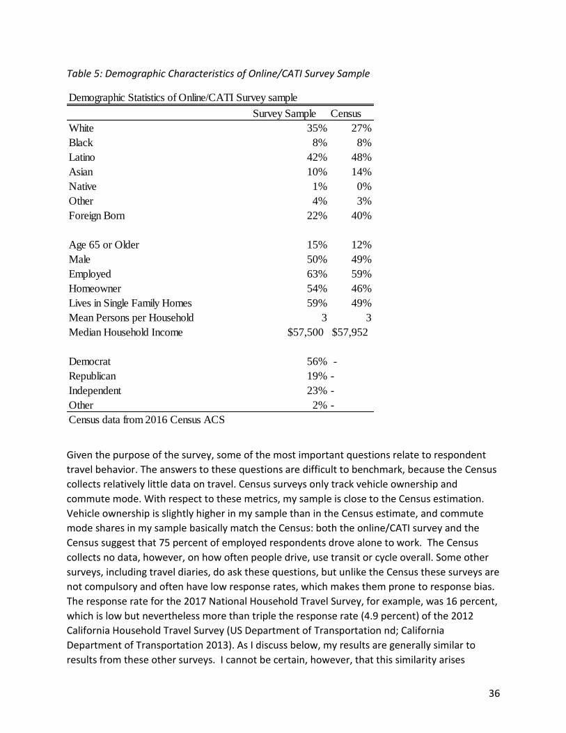
36
Table 5: Demographic Characteristics of Online/CATI Survey Sample
Given the purpose of the survey, some of the most important questions relate to respondent
travel behavior. The answers to these questions are difficult to benchmark, because the Census
collects relatively little data on travel. Census surveys only track vehicle ownership and
commute mode. With respect to these metrics, my sample is close to the Census estimation.
Vehicle ownership is slightly higher in my sample than in the Census estimate, and commute
mode shares in my sample basically match the Census: both the online/CATI survey and the
Census suggest that 75 percent of employed respondents drove alone to work. The Census
collects no data, however, on how often people drive, use transit or cycle overall. Some other
surveys, including travel diaries, do ask these questions, but unlike the Census these surveys are
not compulsory and often have low response rates, which makes them prone to response bias.
The response rate for the 2017 National Household Travel Survey, for example, was 16 percent,
which is low but nevertheless more than triple the response rate (4.9 percent) of the 2012
California Household Travel Survey (US Department of Transportation nd; California
Department of Transportation 2013). As I discuss below, my results are generally similar to
results from these other surveys. I cannot be certain, however, that this similarity arises
Demographic Statistics of Online/CATI Survey sample
Survey Sample Census
White 35% 27%
Black 8% 8%
Latino 42% 48%
Asian 10% 14%
Native 1% 0%
Other 4% 3%
Foreign Born 22% 40%
Age 65 or Older 15% 12%
Male 50% 49%
Employed 63% 59%
Homeowner 54% 46%
Lives in Single Family Homes 59% 49%
Mean Persons per Household 3 3
Median Household Income $57,500 $57,952
Democrat 56% -
Republican 19% -
Independent 23% -
Other 2% -
Census data from 2016 Census ACS
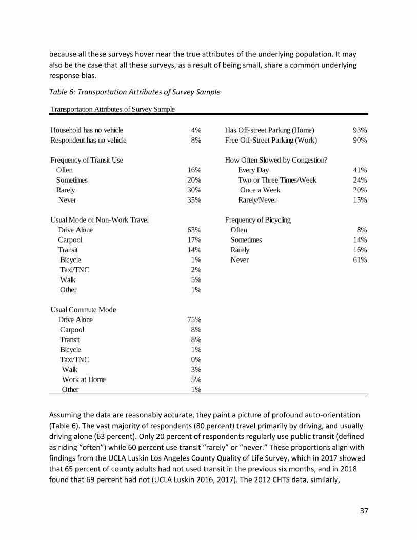
37
because all these surveys hover near the true attributes of the underlying population. It may
also be the case that all these surveys, as a result of being small, share a common underlying
response bias.
Table 6: Transportation Attributes of Survey Sample
Assuming the data are reasonably accurate, they paint a picture of profound auto-orientation
(Table 6). The vast majority of respondents (80 percent) travel primarily by driving, and usually
driving alone (63 percent). Only 20 percent of respondents regularly use public transit (defined
as riding “often”) while 60 percent use transit “rarely” or “never.” These proportions align with
findings from the UCLA Luskin Los Angeles County Quality of Life Survey, which in 2017 showed
that 65 percent of county adults had not used transit in the previous six months, and in 2018
found that 69 percent had not (UCLA Luskin 2016, 2017). The 2012 CHTS data, similarly,
Transportation Attributes of Survey Sample
Household has no vehicle 4% Has Off-street Parking (Home) 93%
Respondent has no vehicle 8% Free Off-Street Parking (Work) 90%
Frequency of Transit Use How Often Slowed by Congestion?
Often 16% Every Day 41%
Sometimes 20% Two or Three Times/Week 24%
Rarely 30% Once a Week 20%
Never 35% Rarely/Never 15%
Usual Mode of Non-Work Travel Frequency of Bicycling
Drive Alone 63% Often 8%
Carpool 17% Sometimes 14%
Transit 14% Rarely 16%
Bicycle 1% Never 61%
Taxi/TNC 2%
Walk 5%
Other 1%
Usual Commute Mode
Drive Alone 75%
Carpool 8%
Transit 8%
Bicycle 1%
Taxi/TNC 0%
Walk 3%
Work at Home 5%
Other 1%
38
suggests that about 73 percent of LA County residents use transit infrequently or not at all
(Manville et al 2018).
Only 11 percent of respondents rely primarily on transit for nonwork travel. Perhaps
unsurprisingly, these transit users are disproportionately concentrated among the small share
of respondents who lack regular access to a private vehicle. Only 16 percent of people with
vehicles report using transit “often” while another 20 percent report using it “sometimes.”
Among people without vehicles, in contrast, 37 percent use transit often and 34 percent use it
sometimes. Note too that while people without vehicles are more likely to use transit, most do
not use transit, a point that reinforces the relative rarity of transit use. Bicycling is even less
common than riding transit. Only 8 percent of respondents reported bicycling often, while 78
percent say they ride a bike rarely or never.
Driving’s prevalence is matched, and probably partly explained, by the prevalence of free
parking. Ninety-three percent of respondents have free off-street parking at their home, while
90 percent of employed respondents can park free at work.17
Although not shown in the table, the sample’s transit riders skew rich. Among respondents who
report riding transit regularly, the median household income is $42,000, more than double the
estimated median household income of LA Metro’s riders. Some of this discrepancy might owe
to the online/CATI survey capturing riders who use systems other than Metro, such as
Metrolink commuter rail, which carries more affluent people. More likely, however, it is a
response bias problem: the regular transit riders who responded to the survey are quite
different economically from transit riders overall.
Support for Measure M
Table 7 shows that the online/CATI survey oversampled voters: 81 percent of respondents said
they voted, while turnout in LA County was only 69 percent. This difference has two likely
sources. First is that survey respondents tend to over-report socially approved behavior (in this
case, to say they voted when they actually didn’t). I address this tendency by using well-tested
language (borrowed from the US National Election Study) when asking if people voted, but
nothing completely eliminates the possibility of false reporting. Second is a selection effect:
people who agree to take surveys tend to be “joiners”, and are thus more likely than the
population at large to be civically and politically active (Keeter et al 2017).
A quarter of respondents reported knowing “a lot” about Measure M before the election, while
30 percent said they knew something about it. Forty-five percent, meanwhile, said they knew
“only a little” or “nothing” about Measure M before Election Day. Among respondents who
17 Table 3, using AHS data, showed slightly lower proportions of LA households with bundled parking. This discrepancy arises for two reasons. First, the AHS survey of Los Angeles includes Orange County. Second and more consequential, the AHS summary data only count garages and carports, while in LA County many housing units come with other forms of offstreet parking. See Manville (2017) for more detailed AHS tabulations of bundled residential parking, which account for other offstreet spaces and are more consonant with the survey data here.
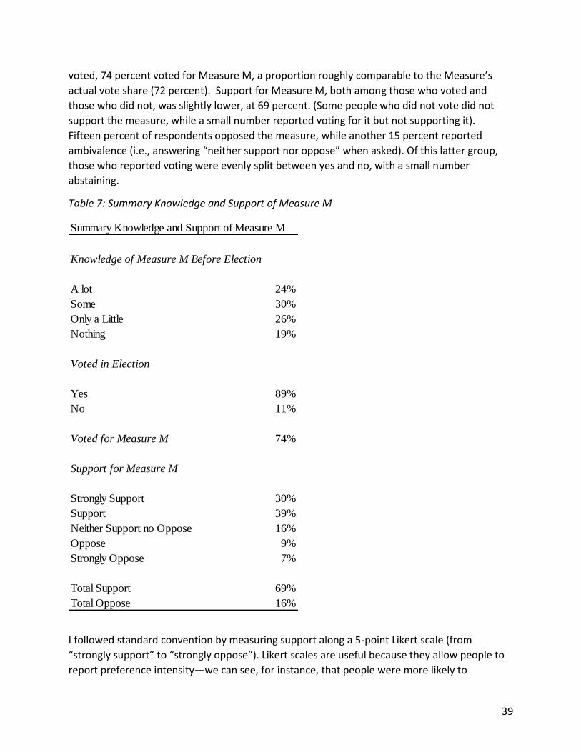
39
voted, 74 percent voted for Measure M, a proportion roughly comparable to the Measure’s
actual vote share (72 percent). Support for Measure M, both among those who voted and
those who did not, was slightly lower, at 69 percent. (Some people who did not vote did not
support the measure, while a small number reported voting for it but not supporting it).
Fifteen percent of respondents opposed the measure, while another 15 percent reported
ambivalence (i.e., answering “neither support nor oppose” when asked). Of this latter group,
those who reported voting were evenly split between yes and no, with a small number
abstaining.
Table 7: Summary Knowledge and Support of Measure M
I followed standard convention by measuring support along a 5-point Likert scale (from
“strongly support” to “strongly oppose”). Likert scales are useful because they allow people to
report preference intensity—we can see, for instance, that people were more likely to
Summary Knowledge and Support of Measure M
Knowledge of Measure M Before Election
A lot 24%
Some 30%
Only a Little 26%
Nothing 19%
Voted in Election
Yes 89%
No 11%
Voted for Measure M 74%
Support for Measure M
Strongly Support 30%
Support 39%
Neither Support no Oppose 16%
Oppose 9%
Strongly Oppose 7%
Total Support 69%
Total Oppose 16%

40
“support” Measure M (39 percent) than “strongly support” it (30 percent). But Likert scales
have two disadvantages. First, some evidence suggests that Likert responses overestimate
extremes. People given a question with a Likert response are more likely to indicate “strong”
support or opposition than if given other ways to report preference intensity (Albaum 1997;
Posner and Weyl 2017). Second, Likert responses are more useful when comparing responses
within people than across them. When a person says they “strongly support” one policy but
only “support” another, we can be confident he or she prefers the first policy to the second. But
when one person reports “strongly supporting” a policy and another reports only “supporting”
it, we are less sure who likes it more, since one person’s strong support might equal to
another’s support. For this reason, in much of this analysis I collapse support and opposition
into binary categories. Unless otherwise noted, I do this for all Likert-style responses in the
survey.
Intercept Survey Descriptive Statistics
The transit rider intercept survey captured 550 total respondents (68 of whom took the survey
in Spanish). Some individual questions had high levels of nonresponse, however, so the typical
question received between 440 and 490 valid responses. The respondents were drawn from 10
different stations, but six of the ten surveyed stations accounted for 80 percent of the
responses. These six stations were served by both bus and rail service. Thirty-seven percent of
total respondents reported riding the bus on the survey day, while another 20 percent said they
would be using rail. The remainder said they would use both. Since rail accounts for about 25
percent of Metro trips overall, the survey probably oversamples rail riders.
Rail riders tend to have a higher socioeconomic status than bus riders, so while the intercept
survey sample is far more disadvantaged than the online/CATI sample, it is less disadvantaged
than Metro’s sample of its overall ridership. The median household income in the intercept
survey is about $25,000, higher than the Metro estimate for transit riders overall (about
$16,000) but roughly equal to metro’s estimate for rail riders ($22,000). About 24 percent of
intercepted transit riders have household incomes below $15,000 per year, well below the 44
percent for Metro riders in general and below the 34 percent estimate for rail riders. My
sample is 17 percent non-Hispanic White, above Metro’s estimate of 11 percent for all riders
but equal to its estimate for rail riders.
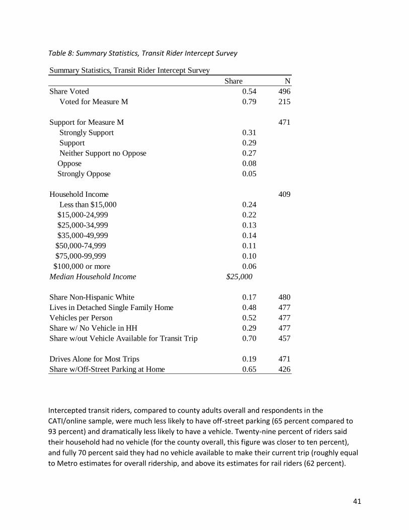
41
Table 8: Summary Statistics, Transit Rider Intercept Survey
Intercepted transit riders, compared to county adults overall and respondents in the
CATI/online sample, were much less likely to have off-street parking (65 percent compared to
93 percent) and dramatically less likely to have a vehicle. Twenty-nine percent of riders said
their household had no vehicle (for the county overall, this figure was closer to ten percent),
and fully 70 percent said they had no vehicle available to make their current trip (roughly equal
to Metro estimates for overall ridership, and above its estimates for rail riders (62 percent).
Summary Statistics, Transit Rider Intercept Survey
Share N
Share Voted 0.54 496
Voted for Measure M 0.79 215
Support for Measure M 471
Strongly Support 0.31
Support 0.29
Neither Support no Oppose 0.27
Oppose 0.08
Strongly Oppose 0.05
Household Income 409
Less than $15,000 0.24
$15,000-24,999 0.22
$25,000-34,999 0.13
$35,000-49,999 0.14
$50,000-74,999 0.11
$75,000-99,999 0.10
$100,000 or more 0.06
Median Household Income $25,000
Share Non-Hispanic White 0.17 480
Lives in Detached Single Family Home 0.48 477
Vehicles per Person 0.52 477
Share w/ No Vehicle in HH 0.29 477
Share w/out Vehicle Available for Transit Trip 0.70 457
Drives Alone for Most Trips 0.19 471
Share w/Off-Street Parking at Home 0.65 426
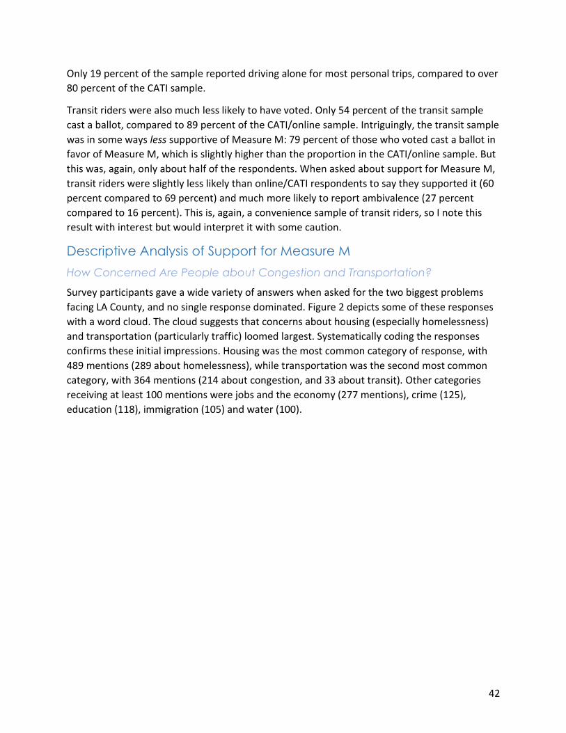
42
Only 19 percent of the sample reported driving alone for most personal trips, compared to over
80 percent of the CATI sample.
Transit riders were also much less likely to have voted. Only 54 percent of the transit sample
cast a ballot, compared to 89 percent of the CATI/online sample. Intriguingly, the transit sample
was in some ways less supportive of Measure M: 79 percent of those who voted cast a ballot in
favor of Measure M, which is slightly higher than the proportion in the CATI/online sample. But
this was, again, only about half of the respondents. When asked about support for Measure M,
transit riders were slightly less likely than online/CATI respondents to say they supported it (60
percent compared to 69 percent) and much more likely to report ambivalence (27 percent
compared to 16 percent). This is, again, a convenience sample of transit riders, so I note this
result with interest but would interpret it with some caution.
Descriptive Analysis of Support for Measure M
How Concerned Are People about Congestion and Transportation?
Survey participants gave a wide variety of answers when asked for the two biggest problems
facing LA County, and no single response dominated. Figure 2 depicts some of these responses
with a word cloud. The cloud suggests that concerns about housing (especially homelessness)
and transportation (particularly traffic) loomed largest. Systematically coding the responses
confirms these initial impressions. Housing was the most common category of response, with
489 mentions (289 about homelessness), while transportation was the second most common
category, with 364 mentions (214 about congestion, and 33 about transit). Other categories
receiving at least 100 mentions were jobs and the economy (277 mentions), crime (125),
education (118), immigration (105) and water (100).
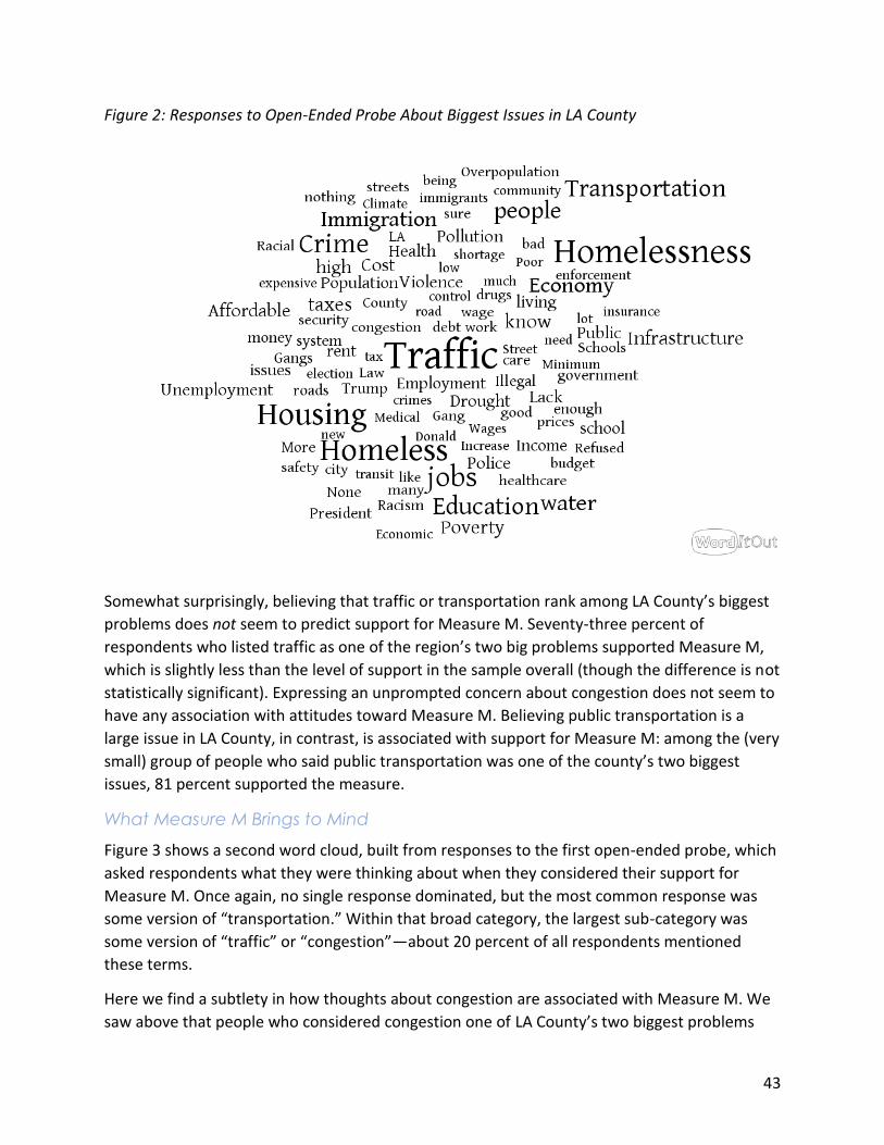
43
Figure 2: Responses to Open-Ended Probe About Biggest Issues in LA County
Somewhat surprisingly, believing that traffic or transportation rank among LA County’s biggest
problems does not seem to predict support for Measure M. Seventy-three percent of
respondents who listed traffic as one of the region’s two big problems supported Measure M,
which is slightly less than the level of support in the sample overall (though the difference is not
statistically significant). Expressing an unprompted concern about congestion does not seem to
have any association with attitudes toward Measure M. Believing public transportation is a
large issue in LA County, in contrast, is associated with support for Measure M: among the (very
small) group of people who said public transportation was one of the county’s two biggest
issues, 81 percent supported the measure.
What Measure M Brings to Mind
Figure 3 shows a second word cloud, built from responses to the first open-ended probe, which
asked respondents what they were thinking about when they considered their support for
Measure M. Once again, no single response dominated, but the most common response was
some version of “transportation.” Within that broad category, the largest sub-category was
some version of “traffic” or “congestion”—about 20 percent of all respondents mentioned
these terms.
Here we find a subtlety in how thoughts about congestion are associated with Measure M. We
saw above that people who considered congestion one of LA County’s two biggest problems
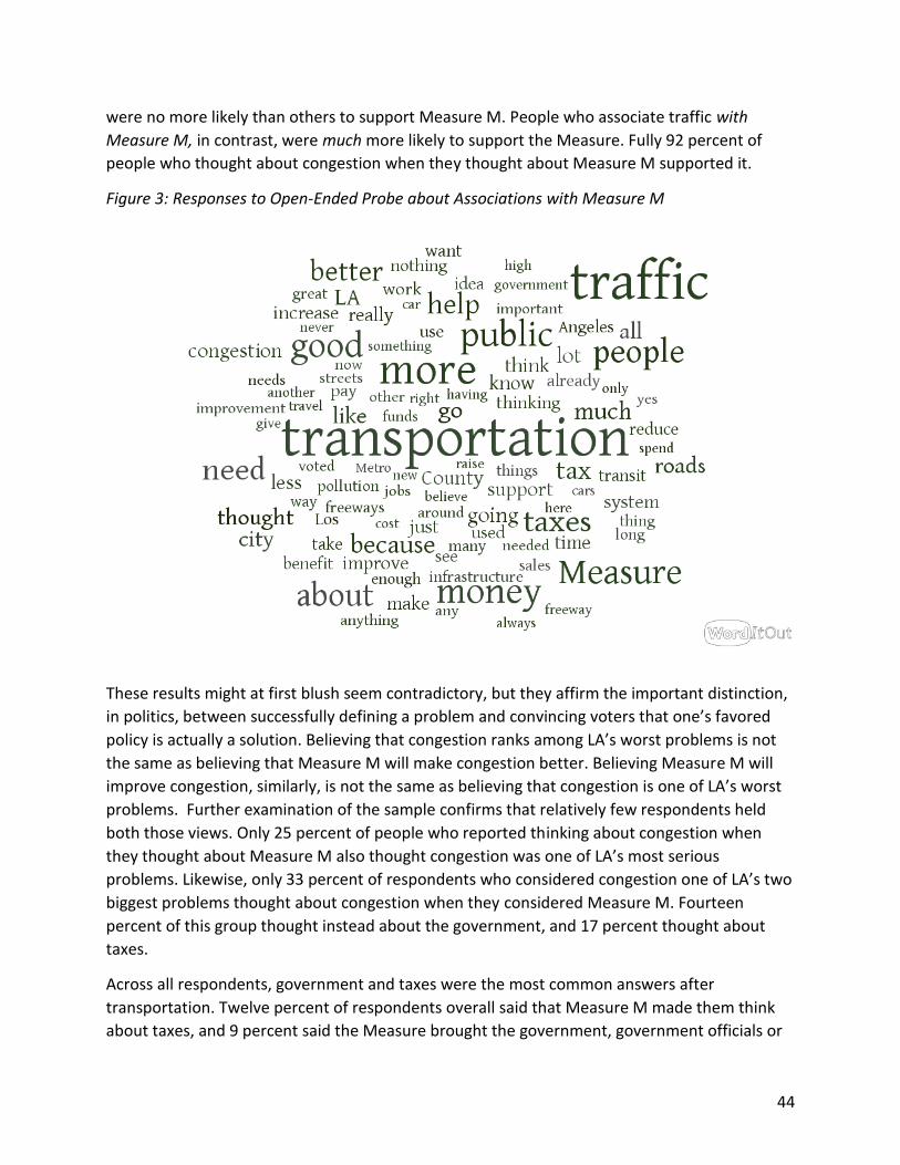
44
were no more likely than others to support Measure M. People who associate traffic with
Measure M, in contrast, were much more likely to support the Measure. Fully 92 percent of
people who thought about congestion when they thought about Measure M supported it.
Figure 3: Responses to Open-Ended Probe about Associations with Measure M
These results might at first blush seem contradictory, but they affirm the important distinction,
in politics, between successfully defining a problem and convincing voters that one’s favored
policy is actually a solution. Believing that congestion ranks among LA’s worst problems is not
the same as believing that Measure M will make congestion better. Believing Measure M will
improve congestion, similarly, is not the same as believing that congestion is one of LA’s worst
problems. Further examination of the sample confirms that relatively few respondents held
both those views. Only 25 percent of people who reported thinking about congestion when
they thought about Measure M also thought congestion was one of LA’s most serious
problems. Likewise, only 33 percent of respondents who considered congestion one of LA’s two
biggest problems thought about congestion when they considered Measure M. Fourteen
percent of this group thought instead about the government, and 17 percent thought about
taxes.
Across all respondents, government and taxes were the most common answers after
transportation. Twelve percent of respondents overall said that Measure M made them think
about taxes, and 9 percent said the Measure brought the government, government officials or
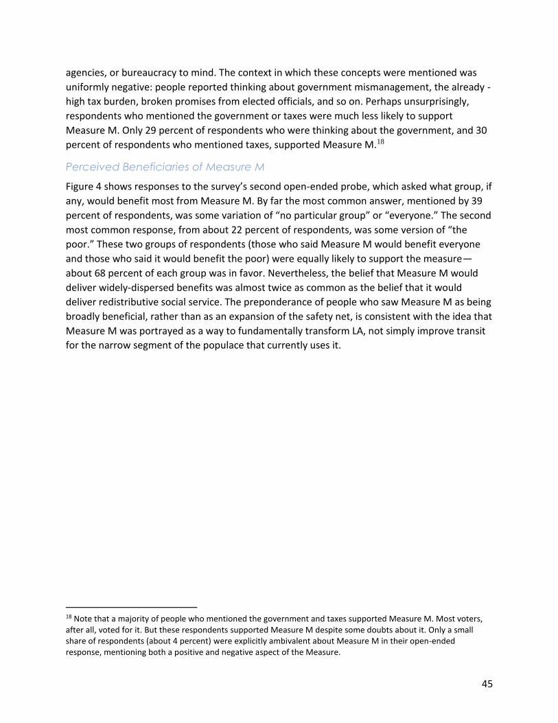
45
agencies, or bureaucracy to mind. The context in which these concepts were mentioned was
uniformly negative: people reported thinking about government mismanagement, the already -
high tax burden, broken promises from elected officials, and so on. Perhaps unsurprisingly,
respondents who mentioned the government or taxes were much less likely to support
Measure M. Only 29 percent of respondents who were thinking about the government, and 30
percent of respondents who mentioned taxes, supported Measure M.18
Perceived Beneficiaries of Measure M
Figure 4 shows responses to the survey’s second open-ended probe, which asked what group, if
any, would benefit most from Measure M. By far the most common answer, mentioned by 39
percent of respondents, was some variation of “no particular group” or “everyone.” The second
most common response, from about 22 percent of respondents, was some version of “the
poor.” These two groups of respondents (those who said Measure M would benefit everyone
and those who said it would benefit the poor) were equally likely to support the measure—
about 68 percent of each group was in favor. Nevertheless, the belief that Measure M would
deliver widely-dispersed benefits was almost twice as common as the belief that it would
deliver redistributive social service. The preponderance of people who saw Measure M as being
broadly beneficial, rather than as an expansion of the safety net, is consistent with the idea that
Measure M was portrayed as a way to fundamentally transform LA, not simply improve transit
for the narrow segment of the populace that currently uses it.
18 Note that a majority of people who mentioned the government and taxes supported Measure M. Most voters, after all, voted for it. But these respondents supported Measure M despite some doubts about it. Only a small share of respondents (about 4 percent) were explicitly ambivalent about Measure M in their open-ended response, mentioning both a positive and negative aspect of the Measure.
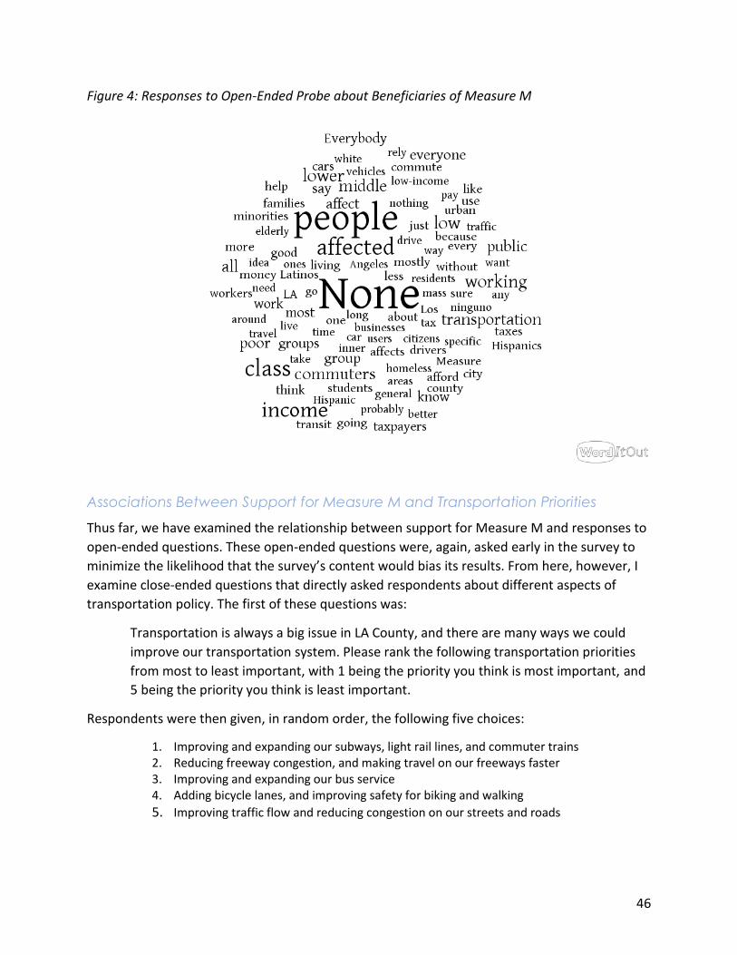
46
Figure 4: Responses to Open-Ended Probe about Beneficiaries of Measure M
Associations Between Support for Measure M and Transportation Priorities
Thus far, we have examined the relationship between support for Measure M and responses to
open-ended questions. These open-ended questions were, again, asked early in the survey to
minimize the likelihood that the survey’s content would bias its results. From here, however, I
examine close-ended questions that directly asked respondents about different aspects of
transportation policy. The first of these questions was:
Transportation is always a big issue in LA County, and there are many ways we could
improve our transportation system. Please rank the following transportation priorities
from most to least important, with 1 being the priority you think is most important, and
5 being the priority you think is least important.
Respondents were then given, in random order, the following five choices:
1. Improving and expanding our subways, light rail lines, and commuter trains 2. Reducing freeway congestion, and making travel on our freeways faster 3. Improving and expanding our bus service 4. Adding bicycle lanes, and improving safety for biking and walking
5. Improving traffic flow and reducing congestion on our streets and roads
47
Table 9 shows the results, for supporters and opponents of Measure M, and for all
respondents. No priority emerges with a clear majority—a testament, perhaps, to the challenge
of marketing a transportation measure in a large region that is both socially and geographically
heterogeneous. Measure M’s supporters were most likely to prioritize improving the rail
system (34 percent), while opponents were most likely to prioritize reducing freeway
congestion (35 percent). Only 20 percent of the Measure’s supporters prioritized expanding the
rail system, and neither group was likely to prioritize bus service, though supporters were
almost twice as likely to do so as opponents (11 percent to 6 percent). Similarly, no group had a
strong appetite for bicycle and pedestrian improvements: only 9 percent prioritized this goal.
Table 9: Transportation Priorities for LA County
Superficially, the results suggest that Measure M supporters prioritized rail while opponents
prioritized congestion. This conclusion, however, is in part an artifact of the survey design. The
survey splits “congestion” into two groups: freeway congestion and congestion on surface
streets. Many Angelinos see these as separate problems, but of course one can argue that
congestion is congestion, and that all congestion concerns should be in one category. The data
offer some support (but hardly definitive evidence) for this view. Forty-seven percent of people
who ranked street congestion as the top priority ranked freeway congestion second most
important, while 50 percent of people who said freeway congestion was most important
ranked street congestion second.
If we do combine the two congestion categories (bottom rows of the table), then people who
prioritize congestion become the largest bloc of both opponents and supporters—though they
are a much larger share of opponents. Forty-eight percent of Measure M supporters prioritize
congestion. Forty-five percent prioritize some sort of transit expansion (over 75 percent of this
support is for rail). Opponents, in contrast, remain much more likely to prioritize congestion (65
percent) and only 26 percent prioritize some sort of transit improvement (and rail, again,
accounts for 75 percent of this support). In sum, reducing congestion appears to be a universal
Most Important Transportation Priority for LA County
(Share of Respondents Ranking "Most Important"
M Supporters Opponents All
Improving and Expanding Rail System 34% 20% 30%
Improving and Expanding Bus Service 11% 6% 9%
Reducing Freeway Congestion 26% 35% 28%
Reducing Street Congestion 22% 30% 24%
Improving Biking and Walking 9% 9% 9%
Congestion (combined) 48% 65% 52%
Transit (combined) 45% 26% 39%
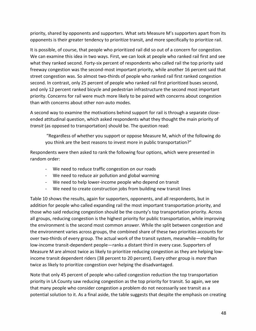
48
priority, shared by opponents and supporters. What sets Measure M’s supporters apart from its
opponents is their greater tendency to prioritize transit, and more specifically to prioritize rail.
It is possible, of course, that people who prioritized rail did so out of a concern for congestion.
We can examine this idea in two ways. First, we can look at people who ranked rail first and see
what they ranked second. Forty-six percent of respondents who called rail the top priority said
freeway congestion was the second-most important priority, while another 16 percent said that
street congestion was. So almost two-thirds of people who ranked rail first ranked congestion
second. In contrast, only 25 percent of people who ranked rail first prioritized buses second,
and only 12 percent ranked bicycle and pedestrian infrastructure the second most important
priority. Concerns for rail were much more likely to be paired with concerns about congestion
than with concerns about other non-auto modes.
A second way to examine the motivations behind support for rail is through a separate close-
ended attitudinal question, which asked respondents what they thought the main priority of
transit (as opposed to transportation) should be. The question read:
“Regardless of whether you support or oppose Measure M, which of the following do
you think are the best reasons to invest more in public transportation?”
Respondents were then asked to rank the following four options, which were presented in
random order:
- We need to reduce traffic congestion on our roads
- We need to reduce air pollution and global warming
- We need to help lower-income people who depend on transit
- We need to create construction jobs from building new transit lines
Table 10 shows the results, again for supporters, opponents, and all respondents, but in
addition for people who called expanding rail the most important transportation priority, and
those who said reducing congestion should be the county’s top transportation priority. Across
all groups, reducing congestion is the highest priority for public transportation, while improving
the environment is the second most common answer. While the split between congestion and
the environment varies across groups, the combined share of these two priorities accounts for
over two-thirds of every group. The actual work of the transit system, meanwhile—mobility for
low-income transit-dependent people—ranks a distant third in every case. Supporters of
Measure M are almost twice as likely to prioritize reducing congestion as they are helping low-
income transit dependent riders (38 percent to 20 percent). Every other group is more than
twice as likely to prioritize congestion over helping the disadvantaged.
Note that only 45 percent of people who called congestion reduction the top transportation
priority in LA County saw reducing congestion as the top priority for transit. So again, we see
that many people who consider congestion a problem do not necessarily see transit as a
potential solution to it. As a final aside, the table suggests that despite the emphasis on creating
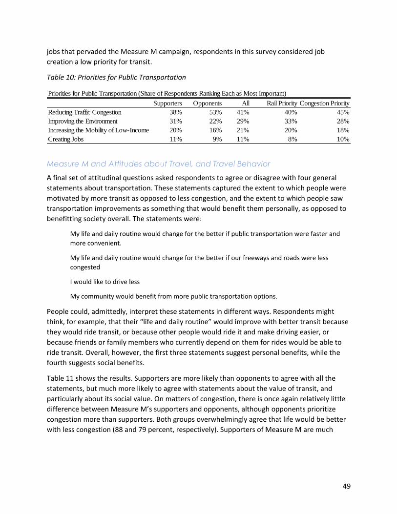
49
jobs that pervaded the Measure M campaign, respondents in this survey considered job
creation a low priority for transit.
Table 10: Priorities for Public Transportation
Measure M and Attitudes about Travel, and Travel Behavior
A final set of attitudinal questions asked respondents to agree or disagree with four general
statements about transportation. These statements captured the extent to which people were
motivated by more transit as opposed to less congestion, and the extent to which people saw
transportation improvements as something that would benefit them personally, as opposed to
benefitting society overall. The statements were:
My life and daily routine would change for the better if public transportation were faster and
more convenient.
My life and daily routine would change for the better if our freeways and roads were less
congested
I would like to drive less
My community would benefit from more public transportation options.
People could, admittedly, interpret these statements in different ways. Respondents might
think, for example, that their “life and daily routine” would improve with better transit because
they would ride transit, or because other people would ride it and make driving easier, or
because friends or family members who currently depend on them for rides would be able to
ride transit. Overall, however, the first three statements suggest personal benefits, while the
fourth suggests social benefits.
Table 11 shows the results. Supporters are more likely than opponents to agree with all the
statements, but much more likely to agree with statements about the value of transit, and
particularly about its social value. On matters of congestion, there is once again relatively little
difference between Measure M’s supporters and opponents, although opponents prioritize
congestion more than supporters. Both groups overwhelmingly agree that life would be better
with less congestion (88 and 79 percent, respectively). Supporters of Measure M are much
Priorities for Public Transportation (Share of Respondents Ranking Each as Most Important)
Supporters Opponents All Rail Priority Congestion Priority
Reducing Traffic Congestion 38% 53% 41% 40% 45%
Improving the Environment 31% 22% 29% 33% 28%
Increasing the Mobility of Low-Income 20% 16% 21% 20% 18%
Creating Jobs 11% 9% 11% 8% 10%
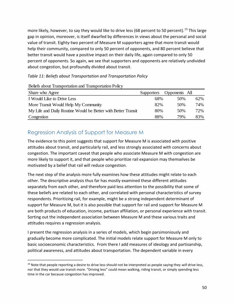
50
more likely, however, to say they would like to drive less (68 percent to 50 percent).19 This large
gap in opinion, moreover, is itself dwarfed by differences in views about the personal and social
value of transit. Eighty-two percent of Measure M supporters agree that more transit would
help their community, compared to only 50 percent of opponents, and 80 percent believe that
better transit would have a positive impact on their daily life, again compared to only 50
percent of opponents. So again, we see that supporters and opponents are relatively undivided
about congestion, but profoundly divided about transit.
Table 11: Beliefs about Transportation and Transportation Policy
Regression Analysis of Support for Measure M
The evidence to this point suggests that support for Measure M is associated with positive
attitudes about transit, and particularly rail, and less strongly associated with concerns about
congestion. The important caveat that people who associate Measure M with congestion are
more likely to support it, and that people who prioritize rail expansion may themselves be
motivated by a belief that rail will reduce congestion.
The next step of the analysis more fully examines how these attitudes might relate to each
other. The descriptive analysis thus far has mostly examined these different attitudes
separately from each other, and therefore paid less attention to the possibility that some of
these beliefs are related to each other, and correlated with personal characteristics of survey
respondents. Prioritizing rail, for example, might be a strong independent determinant of
support for Measure M, but it is also possible that support for rail and support for Measure M
are both products of education, income, partisan affiliation, or personal experience with transit.
Sorting out the independent association between Measure M and these various traits and
attitudes requires a regression analysis.
I present the regression analysis in a series of models, which begin parsimoniously and
gradually become more complicated. The initial models relate support for Measure M only to
basic socioeconomic characteristics. From there I add measures of ideology and partisanship,
political awareness, and attitudes about transportation. The dependent variable in every
19 Note that people reporting a desire to drive less should not be interpreted as people saying they will drive less, nor that they would use transit more. “Driving less” could mean walking, riding transit, or simply spending less time in the car because congestion has improved.
Beliefs about Transportation and Transportation Policy
Share who Agree Supporters Opponents All
I Would Like to Drive Less 68% 50% 62%
More Transit Would Help My Community 82% 50% 74%
My Life and Daily Routine Would be Better with Better Transit 80% 50% 72%
Congestion 88% 79% 83%
51
regression is dichotomous, and coded 1 if a respondent supports Measure M, and zero
otherwise. All the regressions are logits. (Estimating the regressions using other functional
forms does not meaningfully change the results.)
The first three models are shown in Table 12. The models differ slightly from each other; for
purposes of robustness, different models measure the same underlying concept in different
ways (e.g., some account for race with a variable indicating that respondents are White, others
do so with a variable indicating Hispanic/Latino status). Only the third model includes income,
because hundreds of respondents left income blank.20
In general, the three models tell the same story: demographic attributes have little association
with support for Measure M. The exceptions are being employed, riding transit regularly, and
living in a (self-described) urban neighborhood. Stand-alone logit coefficients can be difficult to
interpret, as they suggest changes in log-odds of event (in this case support for Measure M)
occurring. Log-odds are admittedly not an intuitive concept, and thus unhelpful for most
readers. To address this concern, throughout the section I discuss the coefficients differently,
by referring to the association between each variable and its association with the percent
change in the odds of supporting Measure M, controlling for all other factors in the model.
Odds are a slightly more intuitive concept than log-odds, and converting the coefficients in this
way can help readers understand the relative importance of each factor in the model. (I convert
the coefficients to log-odds by exponentiating them, but I do not show this transformation in
the tables).
Both being employed and living in an urban neighborhood increase the odds of supporting
Measure M by about 50 percent, controlling for other variables in the model. Being a regular
transit rider, in contrast, increases the odds of supporting Measure M by 135 percent,
compared to people who do not ride regularly. This association is large, but comes with three
caveats. First is that the sample has very few regular transit riders, so this association, though
strong, can explain only a small portion of Measure M’s success. Second, remember that the
transit riders in this survey are not representative of transit riders overall. Third, the transit
rider variable in this sample is highly correlated with households that lack automobiles. When
the regressions are re-estimated without the transit rider variable, vehicle access becomes a
strong determinant of support for Measure M. So in some ways the transit rider variable might
be proxying for vehicle access.
20 The absence of income data is not as serious of a problem as it might at first seem. Opinions about taxing and spending, and government programs, are influenced by income but the influence tends to be rather small (see Caplan 2007 for a discussion).
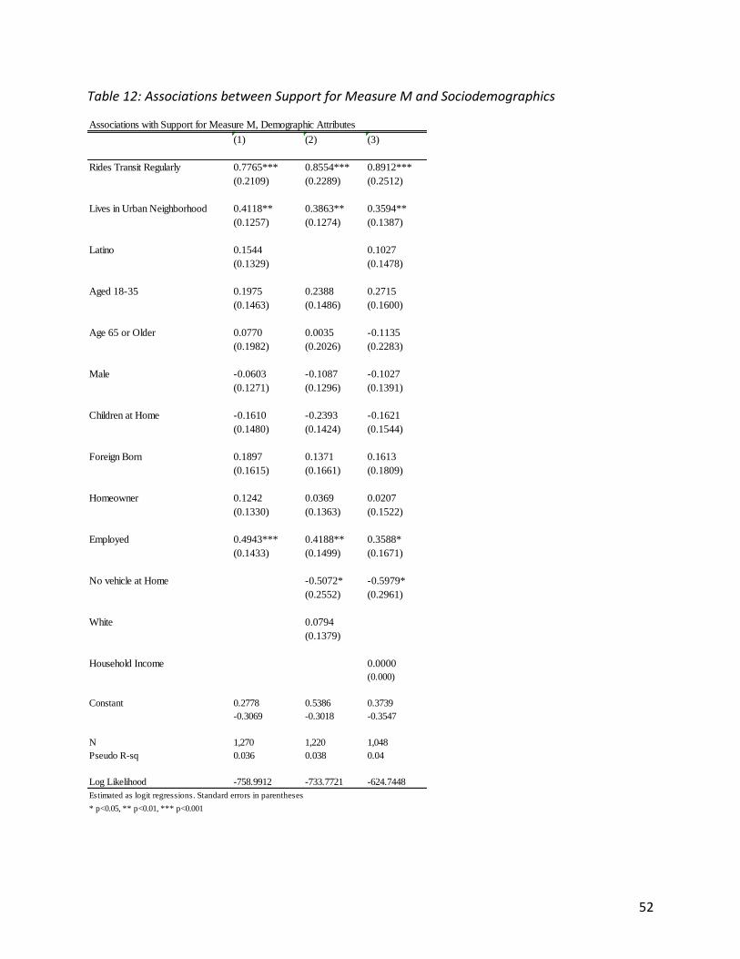
52
Table 12: Associations between Support for Measure M and Sociodemographics
Associations with Support for Measure M, Demographic Attributes
(1) (2) (3)
Rides Transit Regularly 0.7765*** 0.8554*** 0.8912***
(0.2109) (0.2289) (0.2512)
Lives in Urban Neighborhood 0.4118** 0.3863** 0.3594**
(0.1257) (0.1274) (0.1387)
Latino 0.1544 0.1027
(0.1329) (0.1478)
Aged 18-35 0.1975 0.2388 0.2715
(0.1463) (0.1486) (0.1600)
Age 65 or Older 0.0770 0.0035 -0.1135
(0.1982) (0.2026) (0.2283)
Male -0.0603 -0.1087 -0.1027
(0.1271) (0.1296) (0.1391)
Children at Home -0.1610 -0.2393 -0.1621
(0.1480) (0.1424) (0.1544)
Foreign Born 0.1897 0.1371 0.1613
(0.1615) (0.1661) (0.1809)
Homeowner 0.1242 0.0369 0.0207
(0.1330) (0.1363) (0.1522)
Employed 0.4943*** 0.4188** 0.3588*
(0.1433) (0.1499) (0.1671)
No vehicle at Home -0.5072* -0.5979*
(0.2552) (0.2961)
White 0.0794
(0.1379)
Household Income 0.0000
(0.000)
Constant 0.2778 0.5386 0.3739
-0.3069 -0.3018 -0.3547
N 1,270 1,220 1,048
Pseudo R-sq 0.036 0.038 0.04
Log Likelihood -758.9912 -733.7721 -624.7448
Estimated as logit regressions. Standard errors in parentheses
* p<0.05, ** p<0.01, *** p<0.001
53
Table 13 shows the regression estimates that include partisanship and ideology. The first
equations measure ideology; in Model 1 the independent variable of interest is a dichotomous
variable coded 1 if the respondent identifies as liberal and zero otherwise. This variable is both
statistically and practically significant: the coefficient suggests that the odds of supporting
Measure M are 39 percent higher for people who identify as liberal, compared to people who
do not.
The next model exchanges the liberal indicator variable for a variable coded 1 if the respondent
is conservative, and coded zero otherwise. This variable has a moderately large coefficient, but
surprisingly it is positive, and falls slightly shy of the conventional threshold of statistical
significance (the coefficient is significant at the 12 percent level, while conventional thresholds
are usually ten or five percent). One potential explanation for this result lies in conservatism
having a multidimensional and occasionally contradictory nature (Hetherington and Weiler
2009). Some people identify as conservative out of a preference for small government and low
taxes, but others do so because they are traditionalist, religious, and/or have a strong respect
for authority. These preferences needn’t overlap, and we have little reason to think the latter
set of attributes would be associated in any way with Measure M. A variable measuring both
strands of conservatism might be noisy as a result, and yield coefficients that are statistically
insignificant.
To isolate the more libertarian streak of conservatism, the third model replaces the
conservatism measure with a variable constructed from a separate survey question about
government and personal responsibility. The question read as follows:
Thinking about social problems like poverty, pollution and traffic congestion, would you say that
you generally believe the government has a strong responsibility to step in and help solve these
problems, or do you generally believe problems like these will be solved when individuals step
up and change their own behavior?
People could then answer:
1. Government has a responsibility to help solve them
2. Individuals need to take responsibility and change their behavior
I treat people who answer (2) as proponents of smaller government, and conservative in the
libertarian sense. Model 3 uses an indicator variable for this small government attitude, and the
resulting coefficient is large, negative, and statistically significant at the ten percent level. A
belief that people need to help themselves, and not rely on the government, is associated with
a 29 percent reduction in the odds of someone supporting Measure M. Note that the indicator
variable for liberalism remains strong in the presence of this variable, suggesting that liberals
favor Measure M while small government conservatives do not.
The next four models examine partisanship rather than ideology. In my sample, 79 percent of
Democrats supported Measure M, compared to 56 percent of Republicans. As expected, the
partisanship results are much stronger than those associated with ideology. Where identifying
54
as liberal was associated with a 39 percent increase in the odds of supporting Measure M,
identifying as a Democrat was associated with a 164 percent increase in the odds of doing so,
and identifying as a “Strong Democrat” was associated with a 173 percent increase. Identifying
as a Republican, similarly, was associated with opposing Measure M, (a 58 percent decrease in
the odds of support). Being a strong Republican, however, did not intensify opposition. Strong
Republicanism was actually associated with slightly less opposition to Measure M (a 55 percent
reduction in the odds, compared to a 58 percent reduction for Republicans overall). Support for
Measure M, in summary, followed ideological lines, and powerfully followed partisan lines. In
both cases, moreover, the relationship was asymmetrical: liberals and Democrats supported
Measure M more than conservatives and Republicans opposed it.
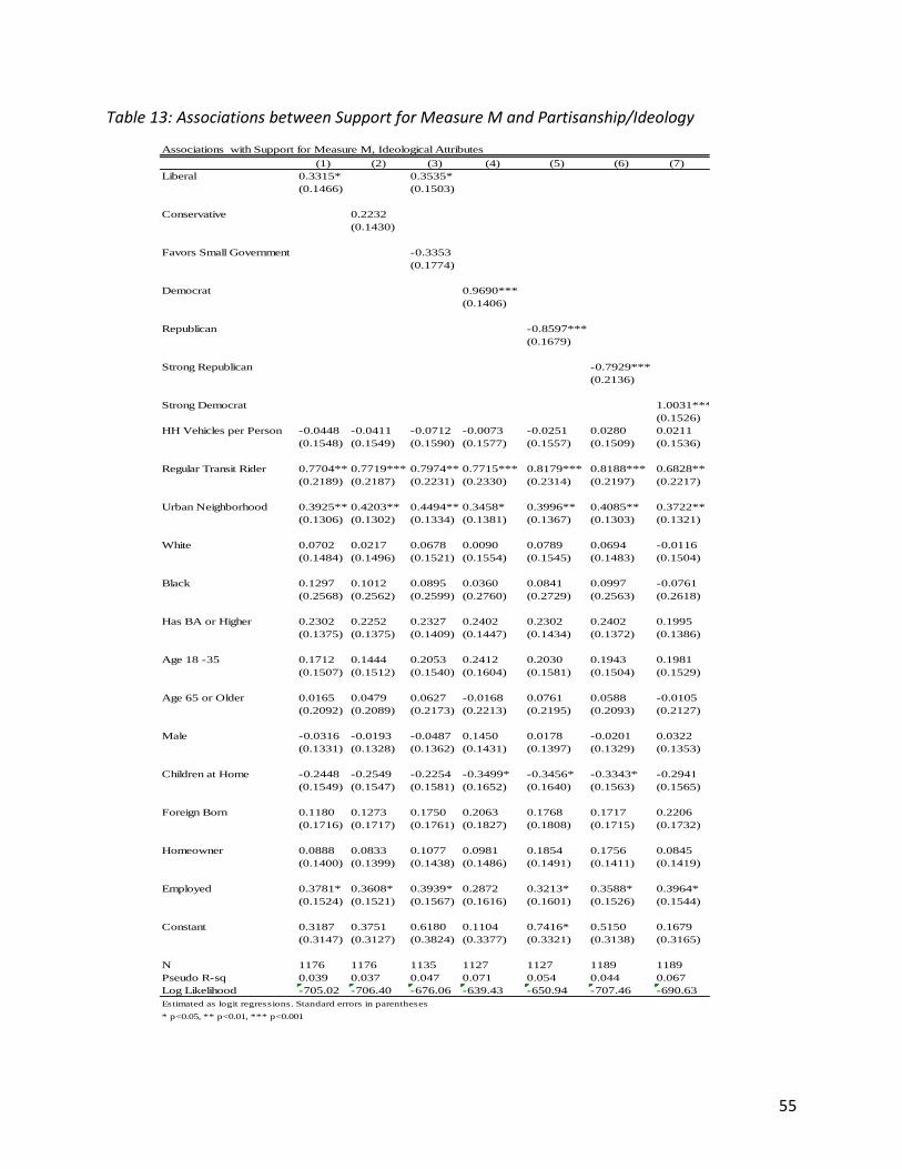
55
Table 13: Associations between Support for Measure M and Partisanship/Ideology
Associations with Support for Measure M, Ideological Attributes
(1) (2) (3) (4) (5) (6) (7)
Liberal 0.3315* 0.3535*
(0.1466) (0.1503)
Conservative 0.2232
(0.1430)
Favors Small Government -0.3353
(0.1774)
Democrat 0.9690***
(0.1406)
Republican -0.8597***
(0.1679)
Strong Republican -0.7929***
(0.2136)
Strong Democrat 1.0031***
(0.1526)
HH Vehicles per Person -0.0448 -0.0411 -0.0712 -0.0073 -0.0251 0.0280 0.0211
(0.1548) (0.1549) (0.1590) (0.1577) (0.1557) (0.1509) (0.1536)
Regular Transit Rider 0.7704***0.7719*** 0.7974***0.7715*** 0.8179*** 0.8188*** 0.6828**
(0.2189) (0.2187) (0.2231) (0.2330) (0.2314) (0.2197) (0.2217)
Urban Neighborhood 0.3925** 0.4203** 0.4494***0.3458* 0.3996** 0.4085** 0.3722**
(0.1306) (0.1302) (0.1334) (0.1381) (0.1367) (0.1303) (0.1321)
White 0.0702 0.0217 0.0678 0.0090 0.0789 0.0694 -0.0116
(0.1484) (0.1496) (0.1521) (0.1554) (0.1545) (0.1483) (0.1504)
Black 0.1297 0.1012 0.0895 0.0360 0.0841 0.0997 -0.0761
(0.2568) (0.2562) (0.2599) (0.2760) (0.2729) (0.2563) (0.2618)
Has BA or Higher 0.2302 0.2252 0.2327 0.2402 0.2302 0.2402 0.1995
(0.1375) (0.1375) (0.1409) (0.1447) (0.1434) (0.1372) (0.1386)
Age 18 -35 0.1712 0.1444 0.2053 0.2412 0.2030 0.1943 0.1981
(0.1507) (0.1512) (0.1540) (0.1604) (0.1581) (0.1504) (0.1529)
Age 65 or Older 0.0165 0.0479 0.0627 -0.0168 0.0761 0.0588 -0.0105
(0.2092) (0.2089) (0.2173) (0.2213) (0.2195) (0.2093) (0.2127)
Male -0.0316 -0.0193 -0.0487 0.1450 0.0178 -0.0201 0.0322
(0.1331) (0.1328) (0.1362) (0.1431) (0.1397) (0.1329) (0.1353)
Children at Home -0.2448 -0.2549 -0.2254 -0.3499* -0.3456* -0.3343* -0.2941
(0.1549) (0.1547) (0.1581) (0.1652) (0.1640) (0.1563) (0.1565)
Foreign Born 0.1180 0.1273 0.1750 0.2063 0.1768 0.1717 0.2206
(0.1716) (0.1717) (0.1761) (0.1827) (0.1808) (0.1715) (0.1732)
Homeowner 0.0888 0.0833 0.1077 0.0981 0.1854 0.1756 0.0845
(0.1400) (0.1399) (0.1438) (0.1486) (0.1491) (0.1411) (0.1419)
Employed 0.3781* 0.3608* 0.3939* 0.2872 0.3213* 0.3588* 0.3964*
(0.1524) (0.1521) (0.1567) (0.1616) (0.1601) (0.1526) (0.1544)
Constant 0.3187 0.3751 0.6180 0.1104 0.7416* 0.5150 0.1679
(0.3147) (0.3127) (0.3824) (0.3377) (0.3321) (0.3138) (0.3165)
N 1176 1176 1135 1127 1127 1189 1189
Pseudo R-sq 0.039 0.037 0.047 0.071 0.054 0.044 0.067
Log Likelihood -705.02 -706.40 -676.06 -639.43 -650.94 -707.46 -690.63
Estimated as logit regressions. Standard errors in parentheses
* p<0.05, ** p<0.01, *** p<0.001
56
The next two models (Table 14) keep the Democratic indicator variable, and add two more
independent variables of interest: a dichotomous variable coded 1 if a respondent reported
knowing a lot about Measure M prior to the election, and (in the second model) a variable
coded 1 if the respondent thought LA County was “going in the right direction.” In the first of
these models, the knowledge-of-Measure-M variable is positive but not statistically significant.
In the second, which includes the direction-of-county variable, shows both variables as positive
and statistically significant. This latter model suggests that, controlling for other factors, the
odds of supporting Measure M were 42 percent greater for people who knew a lot about it,
while believing the county was going in the right direction was associated with a very large (187
percent) increase in the odds of supporting Measure M.
For two reasons, I view these results skeptically. First, the electoral knowledge coefficient is
unstable. If prior knowledge was truly associated with support for Measure M, we would see
that in models with fewer variables. A coefficient that jumps dramatically in size when another
variable is added is probably capturing more noise than signal. While I am not saying that that
electoral knowledge was immaterial, I think this regression estimate is probably an unreliable
guide to its magnitude.
My second reason for skepticism is a concern about endogeneity. I administered the survey
after the election, so the causal relationship between support for Measure M and opinions
about the direction of the County might run two ways. People who believed the County was
going in the right direction may have been more likely to support an ambitious plan like
Measure M, but some people may have thought the County was going in the right direction
because it had supported an ambitious plan like Measure M. My data offer no way to
distinguish between these views, so the coefficient associated with the direction of the county
may reflect both cause and effect.
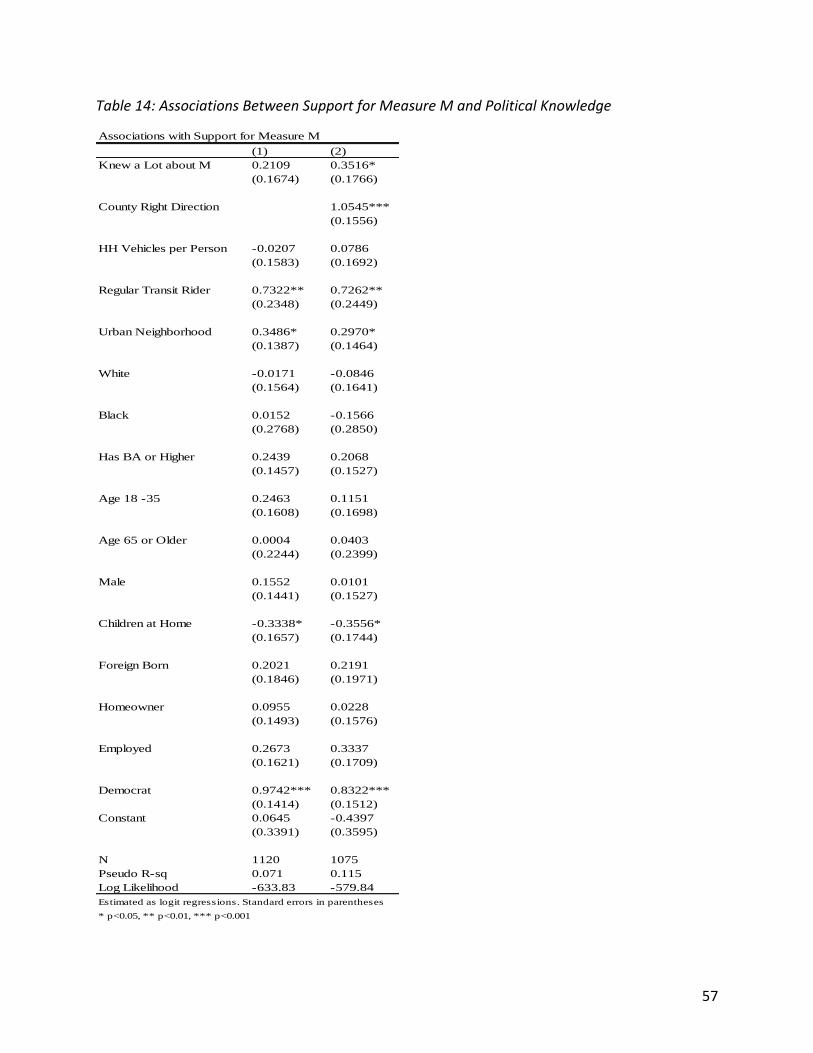
57
Table 14: Associations Between Support for Measure M and Political Knowledge
Associations with Support for Measure M
(1) (2)
Knew a Lot about M 0.2109 0.3516*
(0.1674) (0.1766)
County Right Direction 1.0545***
(0.1556)
HH Vehicles per Person -0.0207 0.0786
(0.1583) (0.1692)
Regular Transit Rider 0.7322** 0.7262**
(0.2348) (0.2449)
Urban Neighborhood 0.3486* 0.2970*
(0.1387) (0.1464)
White -0.0171 -0.0846
(0.1564) (0.1641)
Black 0.0152 -0.1566
(0.2768) (0.2850)
Has BA or Higher 0.2439 0.2068
(0.1457) (0.1527)
Age 18 -35 0.2463 0.1151
(0.1608) (0.1698)
Age 65 or Older 0.0004 0.0403
(0.2244) (0.2399)
Male 0.1552 0.0101
(0.1441) (0.1527)
Children at Home -0.3338* -0.3556*
(0.1657) (0.1744)
Foreign Born 0.2021 0.2191
(0.1846) (0.1971)
Homeowner 0.0955 0.0228
(0.1493) (0.1576)
Employed 0.2673 0.3337
(0.1621) (0.1709)
Democrat 0.9742*** 0.8322***
(0.1414) (0.1512)
Constant 0.0645 -0.4397
(0.3391) (0.3595)
N 1120 1075
Pseudo R-sq 0.071 0.115
Log Likelihood -633.83 -579.84
Estimated as logit regressions. Standard errors in parentheses
* p<0.05, ** p<0.01, *** p<0.001
58
The final regression equations include variables that measure beliefs about transportation,
transit and congestion, as well as variables that measure exposure to congestion (Table 15).
Taken together, these models reinforce many of the findings from the descriptive analysis
above. Concerns about congestion again seem to have no consistent association with support
for Measure M. There is no statistically significant relationship between support for Measure M
and thinking congestion is one of the county’s biggest problems, or between support for
Measure M thinking the county’s top transportation priority should be congestion reduction, or
between support for Measure M and being slowed down by congestion at least once a day, or
between support for Measure M and thinking life would be better with less congestion (this last
coefficient, in fact, is statistically significant and negative in some models, though never large).
People who thought about congestion when thinking about Measure M were, however,
extremely likely to support the measure. Mentally linking Measure M to congestion was
associated with a 555 percent increase in the odds of supporting Measure M, even after
controlling for a wide range of sociological and ideological factors.
One way to interpret this strong relationship between supporting Measure M and associating it
with congestion is that people who associate Measure M with congestion think Measure M can
help solve congestion. Since Measure M was primarily about transit, this association can thus
be plausibly interpreted as a belief that transit will help solve LA’s congestion problems. The
next few regressions provide indirect support for this interpretation, by showing that positive
beliefs about transit were powerfully correlated with Measure M. Thinking about transit when
thinking about Measure M was associated with a 1200 percent increase in the odds of
supporting Measure M. (Recall, however, that only a tiny fraction of respondents reported this
thought). Prioritizing transit as a transportation goal was associated with a 153 percent increase
in the odds of supporting Measure M. Believing transit would help the community was
associated with a roughly 160 percent increase in the odds.
It is not clear, however, that these positive beliefs about transit were related to any short-term
desire to use it. The survey asked people how long, in minutes, it would take them to walk to
their nearest transit stop. People who believed they lived closer to transit were no more likely
to support Measure M, and neither were people who reported wanting to drive less.
Finally, although these models are not shown in the table (to conserve space), variables
indicating that respondents believed the poor would be the primary beneficiaries of Measure M
had no statistically significant association with support for the measure, and neither did a
variable indicating the respondent’s belief that transit’s top priority should be helping low-
income people.
Table 15 : Associations Between Support for Measure M and Beliefs about Transportation
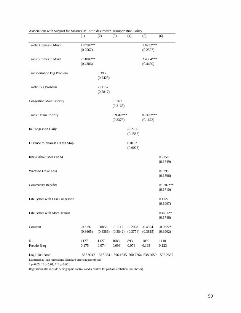
59
Associations with Support for Measure M: Attitudes toward Transportation Policy
(1) (2) (3) (4) (5) (6)
Traffic Comes to Mind 1.8794*** 1.8732***
(0.2567) (0.2597)
Transit Comes to Mind 2.5804*** 2.4564***
(0.4386) (0.4430)
Transportation Big Problem 0.3950
(0.2428)
Traffic Big Problem -0.1157
(0.2817)
Congestion Main Priority 0.1023
(0.2168)
Transit Main Priority 0.9318*** 0.7472***
(0.2376) (0.1672)
In Congestion Daily -0.2766
(0.1586)
Distance to Nearest Transit Stop 0.0102
(0.0073)
Knew About Measure M 0.2150
(0.1749)
Wants to Drive Less 0.0795
(0.1596)
Community Benefits 0.9782***
(0.1710)
Life Better with Less Congestion 0.1122
(0.1997)
Life Better with More Transit 0.4516**
(0.1746)
Constant -0.3192 0.0858 -0.1112 -0.2028 -0.4904 -0.9622*
(0.3665) (0.3386) (0.3842) (0.3774) (0.3815) (0.3902)
N 1127 1127 1083 893 1099 1110
Pseudo R-sq 0.175 0.074 0.093 0.078 0.193 0.123
Log Likelihood -567.9042 -637.3641 -596.1535 -500.7264 -538.0659 -592.2685
Estimated as logit regressions. Standard errors in parentheses
* p<0.05, ** p<0.01, *** p<0.001.
Regressions also include demographic controls and a control for partisan affiliation (not shown).
60
Measure M and Support for Transit-Complementary Policies
The second section of this report summarized evidence suggesting that building transit will not,
by itself, lead to large increases in transit ridership. Effective transit often requires a dense built
environment, which serves the dual purpose of making transit more effective and driving more
difficult. Transit-friendly built environments have more housing and less parking. On both
measures, compared to the legacy transit regions of the US, Los Angeles falls short. Thus, the
ultimate efficacy of Measure M’s transit investments may well hinge on LA’s adoption of
complementary policies that increase its density and reduce the extent to which its built
environment accommodates driving.
Reforms of this sort will almost certainly be less popular than Measure M. In part this difference
in popularity will arise because policymakers and elected officials have spent decades extolling
the virtues of transit, while the virtues of less parking or more density have played less of a role
in public discourse. But Measure M is also more popular because it offered voters a
fundamentally different bargain. Measure M promised new amenities for existing residents—
more road and transit investments—and did so on the premise that these amenities would
make driving easier. Increasing density and reducing the rate at which the region adds parking,
in contrast, would help future residents, and make the transit system effective, but could make
driving for existing residents harder. In part because of concerns about congestion, both
housing development and parking reform are fault lines in local politics. Residents of LA County,
and particularly of its more urban areas, are highly divided about housing development, and
highly sensitive to the supply of parking.
I examined people’s willingness to support housing and parking reforms by asking respondents
to agree or disagree with a series of statements about parking requirements and residential
development. Much of LA’s parking supply is an artifact of the region’s comparatively high
minimum parking requirements (Manville et al 2013). Parking requirements are a powerful but
also largely hidden aspect of urban development, so I assumed that at least some respondents
were not aware of them. The survey thus first summarized parking requirements briefly, and
suggested that they are a source of debate:
One issue that always gets a lot of attention is parking. Currently, when developers build
housing in LA County, cities require them to include parking spaces for residents and visitors.
These parking requirements can be controversial, and some cities might remove them. Thinking
about these parking requirements, please tell us how much you agree or disagree with the
following statements:
Respondents were then presented with the following sentences, in random order:
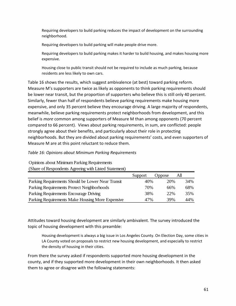
61
Requiring developers to build parking reduces the impact of development on the surrounding
neighborhood.
Requiring developers to build parking will make people drive more.
Requiring developers to build parking makes it harder to build housing, and makes housing more
expensive.
Housing close to public transit should not be required to include as much parking, because
residents are less likely to own cars.
Table 16 shows the results, which suggest ambivalence (at best) toward parking reform.
Measure M’s supporters are twice as likely as opponents to think parking requirements should
be lower near transit, but the proportion of supporters who believe this is still only 40 percent.
Similarly, fewer than half of respondents believe parking requirements make housing more
expensive, and only 35 percent believe they encourage driving. A large majority of respondents,
meanwhile, believe parking requirements protect neighborhoods from development, and this
belief is more common among supporters of Measure M than among opponents (70 percent
compared to 66 percent). Views about parking requirements, in sum, are conflicted: people
strongly agree about their benefits, and particularly about their role in protecting
neighborhoods. But they are divided about parking requirements’ costs, and even supporters of
Measure M are at this point reluctant to reduce them.
Table 16: Opinions about Minimum Parking Requirements
Attitudes toward housing development are similarly ambivalent. The survey introduced the
topic of housing development with this preamble:
Housing development is always a big issue in Los Angeles County. On Election Day, some cities in
LA County voted on proposals to restrict new housing development, and especially to restrict
the density of housing in their cities.
From there the survey asked if respondents supported more housing development in the
county, and if they supported more development in their own neighborhoods. It then asked
them to agree or disagree with the following statements:
Opinions about Minimum Parking Requirements
(Share of Respondents Agreeing with Listed Statement)
Support Oppose All
Parking Requirements Should be Lower Near Transit 40% 20% 34%
Parking Requirements Protect Neighborhoods 70% 66% 68%
Parking Requirements Encourage Driving 38% 22% 35%
Parking Requirements Make Housing More Expensive 47% 39% 44%
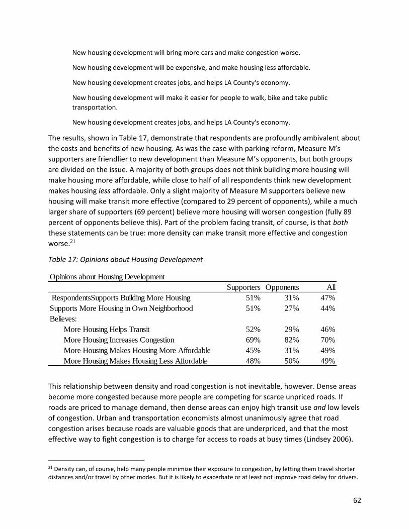
62
New housing development will bring more cars and make congestion worse.
New housing development will be expensive, and make housing less affordable.
New housing development creates jobs, and helps LA County's economy.
New housing development will make it easier for people to walk, bike and take public
transportation.
New housing development creates jobs, and helps LA County's economy.
The results, shown in Table 17, demonstrate that respondents are profoundly ambivalent about
the costs and benefits of new housing. As was the case with parking reform, Measure M’s
supporters are friendlier to new development than Measure M’s opponents, but both groups
are divided on the issue. A majority of both groups does not think building more housing will
make housing more affordable, while close to half of all respondents think new development
makes housing less affordable. Only a slight majority of Measure M supporters believe new
housing will make transit more effective (compared to 29 percent of opponents), while a much
larger share of supporters (69 percent) believe more housing will worsen congestion (fully 89
percent of opponents believe this). Part of the problem facing transit, of course, is that both
these statements can be true: more density can make transit more effective and congestion
worse.21
Table 17: Opinions about Housing Development
This relationship between density and road congestion is not inevitable, however. Dense areas
become more congested because more people are competing for scarce unpriced roads. If
roads are priced to manage demand, then dense areas can enjoy high transit use and low levels
of congestion. Urban and transportation economists almost unanimously agree that road
congestion arises because roads are valuable goods that are underpriced, and that the most
effective way to fight congestion is to charge for access to roads at busy times (Lindsey 2006).
21 Density can, of course, help many people minimize their exposure to congestion, by letting them travel shorter distances and/or travel by other modes. But it is likely to exacerbate or at least not improve road delay for drivers.
Opinions about Housing Development
Supporters Opponents All
RespondentsSupports Building More Housing 51% 31% 47%
Supports More Housing in Own Neighborhood 51% 27% 44%
Believes:
More Housing Helps Transit 52% 29% 46%
More Housing Increases Congestion 69% 82% 70%
More Housing Makes Housing More Affordable 45% 31% 49%
More Housing Makes Housing Less Affordable 48% 50% 49%
63
Substantial evidence also suggests that when governments use congestion pricing, the result is
not just less congestion but dramatically increased transit ridership, and ridership by former
drivers (Small 2004; Santos 2008; Christiansen 2006). A final advantage of congestion charging
is the speed with which it is effective. Parking and zoning reform are important, but can also
take years to bear fruit, since most of the built environment already exists, and new
development in a large city—even when occurring at a brisk pace—rarely accounts for more
than 2 percent of the housing stock each year (in recent years, annual development in LA has
accounted for about ½ of one percent of the total housing stock). Road pricing, in contrast,
immediately injects a powerful incentive to use transit more and drive less. Where the built
environments in New York, Boston and San Francisco function as a shadow tax on driving—one
that took decades to create—road pricing offers a faster, more direct and more transparent
path to the same outcome.
Given these advantages, and given the widespread concern about traffic congestion in Los
Angeles County, the survey asked respondents about congestion charging. As was the case with
parking requirements, I assumed most respondents would not be familiar with pricing, and so
first introduced the concept before asking about it:
Some transportation officials argue that the best solution to LA County's traffic congestion is to
make driving more expensive at busy times. For example, if we had tolls on our freeways that
were higher when many people wanted to drive, such as at rush hour, congestion would go
down. Would you support or oppose using tolls like this on LA County's freeways?
Figure 5 shows the results. Congestion pricing, unsurprisingly, is not popular. On the positive
side, supporters of Measure M are far more likely than opponents to support road pricing, but
support is still only at 38 percent (compared to 72 percent for Measure M.) Among opponents,
support is only 16 percent.
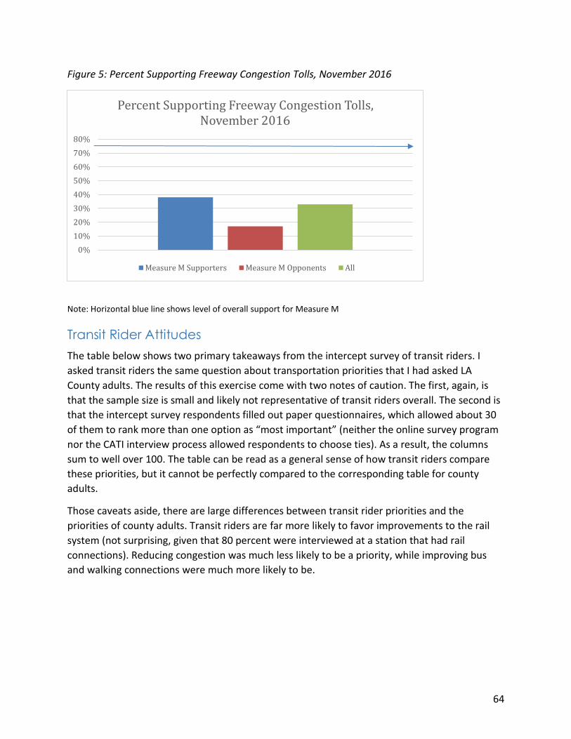
64
Figure 5: Percent Supporting Freeway Congestion Tolls, November 2016
Note: Horizontal blue line shows level of overall support for Measure M
Transit Rider Attitudes
The table below shows two primary takeaways from the intercept survey of transit riders. I
asked transit riders the same question about transportation priorities that I had asked LA
County adults. The results of this exercise come with two notes of caution. The first, again, is
that the sample size is small and likely not representative of transit riders overall. The second is
that the intercept survey respondents filled out paper questionnaires, which allowed about 30
of them to rank more than one option as “most important” (neither the online survey program
nor the CATI interview process allowed respondents to choose ties). As a result, the columns
sum to well over 100. The table can be read as a general sense of how transit riders compare
these priorities, but it cannot be perfectly compared to the corresponding table for county
adults.
Those caveats aside, there are large differences between transit rider priorities and the
priorities of county adults. Transit riders are far more likely to favor improvements to the rail
system (not surprising, given that 80 percent were interviewed at a station that had rail
connections). Reducing congestion was much less likely to be a priority, while improving bus
and walking connections were much more likely to be.
0%
10%
20%
30%
40%
50%
60%
70%
80%
Percent Supporting Freeway Congestion Tolls, November 2016
Measure M Supporters Measure M Opponents All
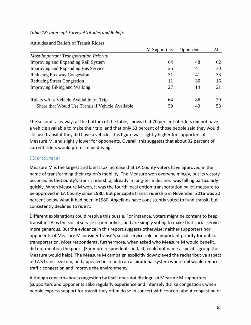
65
Table 18: Intercept Survey Attitudes and Beliefs
The second takeaway, at the bottom of the table, shows that 70 percent of riders did not have
a vehicle available to make their trip, and that only 53 percent of those people said they would
still use transit if they did have a vehicle. This figure was slightly higher for supporters of
Measure M, and slightly lower for opponents. Overall, this suggests that about 32 percent of
current riders would prefer to be driving.
Conclusion
Measure M is the largest and latest tax increase that LA County voters have approved in the
name of transforming their region’s mobility. The Measure won overwhelmingly, but its victory
occurred as theCounty’s transit ridership, already in long-term decline, was falling particularly
quickly. When Measure M won, it was the fourth local option transportation ballot measure to
be approved in LA County since 1980. But per capita transit ridership in November 2016 was 20
percent below what it had been in1980. Angelinos have consistently voted to fund transit, but
consistently declined to ride it.
Different explanations could resolve this puzzle. For instance, voters might be content to keep
transit in LA as the social service it primarily is, and are simply voting to make that social service
more generous. But the evidence in this report suggests otherwise: neither supporters nor
opponents of Measure M consider transit’s social service role an important priority for public
transportation. Most respondents, furthermore, when asked who Measure M would benefit,
did not mention the poor. (Far more respondents, in fact, could not name a specific group the
Measure would help). The Measure M campaign explicitly downplayed the redistributive aspect
of LA’s transit system, and appealed instead to an aspirational system where rail would reduce
traffic congestion and improve the environment.
Although concern about congestion by itself does not distinguish Measure M supporters
(supporters and opponents alike regularly experience and intensely dislike congestion), when
people express support for transit they often do so in concert with concern about congestion or
Attitudes and Beliefs of Transit Riders
M Supporters Opponents All
Most Important Transportation Priority
Improving and Expanding Rail System 64 48 62
Improving and Expanding Bus Service 25 41 30
Reducing Freeway Congestion 31 41 33
Reducing Street Congestion 11 36 16
Improving Biking and Walking 27 14 21
Riders w/out Vehicle Available for Trip 64 86 70
Share that Would Use Transit if Vehicle Available 59 49 53
66
the environment. Three-quarters of Measure M supporters see transit’s top priority as either
reducing congestion or reducing pollution, and the typical Measure M supporter, when asked
to rank the county’s transportation priorities, usually named building rail first and reducing
congestion second. Other non-auto modes, like buses or bike lanes, lagged far behind in
people’s priorities.
Another powerful driver of support for Measure M was partisanship. Simply being a Democrat
was strongly associated with support for Measure M, dwarfing other personal attributes—
urban location, income, race, regular experience riding transit, or regular experience being in
congestion. The growing partisanship of transportation issues documented elsewhere appears
to be alive and well in Los Angeles County.
All of these conclusions come with a broad set of caveats. Survey research is imperfect, and the
surveys I conducted have shortcomings. I have oversampled affluent people and undersampled
Latinos, and my survey of transit riders was a simple convenience sample. Some of the survey
responses could be interpreted in more than one way, as I have detailed in the report. So
certaintly nothing here is definitive. At the same time, the survey did allow me to test the same
ideas in different ways, and the results are generally consistent.
Assuming the findings in this report are broadly accurate, they offer at least the contours of an
explanation for why transit ballots can win without spurring transit ridership. Linking transit to
Democratic identity is powerful politically, but its political power arises precisely because it
divorces transit from the realm of material self-interest, and especially from the realm of
personal transportation. When transit becomes a box that Democrats will reliably check, it
gains votes. But the more these votes are indicative of Democratic identity, the less likely they
are to suggest anything about travel behavior. Similarly, linking rail transit to traffic reduction
strongly implies that transit will benefit people in their role as drivers. This again is powerful
politically; regions like Los Angeles have far more drivers than transit riders, and as this report
has shown, drivers are much more likely to vote. But a vote for transit motivated by a desire to
continue driving also suggests that as transit service expands travel behavior will not change.
Adding to all this, of course, is that the typical Measure M supporter has few of the hallmarks of
a transit rider: he or she owns vehicles, and has access to parking at home or work.
One might argue that LA’s transit investments are intended to create future change—that votes
for transit today will translate into travel behavior changes by the Angelinos of ten or twenty
years from now. Certainly one hopes this is the case, and it cannot be ruled out. But Los
Angeles, again, has been expandings its transit system for almost 30 years, and during that time
its ridership has fallen. While it is possible that the system simply needs to hit a “tipping point”
where it will have enough connections to reverse ridership declines and trigger large increases
in use, it seems unwise to count on such a scenario. A look at other regions suggests that non-
poor people use transit when driving is expensive or otherwise inconvenient, and when land
uses truly support transit. In practice this means denser housing development, less required
parking, and—in some international cities—tolling roads to combat congestion. These changes
67
are very different, and much more controversial, than raising countywide sales taxes. They
involve decisions about how we allocate scarce space in particular locations. While supporters
of Measure M are more supportive of these policies than are Measure M’s opponents, overall
support remains low—which may not be surprising, given that these policies make driving
either harder or more expensive, and Measure M implicitly promised the opposite.
Measure M, in sum, demonstrated Angelinos’ strong willingness and consensus about financing
transit, but the magnitude of its victory might conceal the extent of the latent conflict that
surrounds the additional policies needed to make transit work. Political battles over revenue
cannot, by themselves, create a great transit system. Transit systems also require conflicts over
the allocation of space, and these conflicts are often much harder fought.
For transit advocates in Los Angeles, the best course of action now might be to begin the
process of education about what makes transit effective, and what transit can and cannot do. A
transit system cannot clear the roads for drivers; a look at any of the world’s great transit cities
quickly confirms that fact. Transit can transform cities in ways that make them more livable,
that enable and foster more inclusive and varied built enviornments, and that let people move
around in more and healthier ways, reducing their everyday experience with road traffic
congestion. But these require changes in how the city uses space. The fiscal change of
increasing a sales tax is an undeniable political accomplishment, but only the first and arguably
the easiest step in creating a transit-oriented region.
68
References
Albaum, Gerald. 1997. The Likert Scale Revisited. Journal of the Market Research Society.
39(2):331.
Aldrich, John. 1995. Why Parties? Chicago: University of Chicago Press.
APTA (American Public Transportation Association). 2016. Update: 2016 Ballot Measures.
http://www.apta.com/mediacenter/pressreleases/2016/Pages/2016-Ballot-Measures.aspx
APTA. 2008 and 2016. Public Transportation Fact Book. Washington, DC: American Public
Transportation Association.
APTA, nda. Public Transportation Use is Growing: Here are the Facts. Washington, DC.
https://www.apta.com/mediacenter/ptbenefits/Pages/default.aspx
APTA, ndb. Public Transportation Reduces Greenhouse Gases and Conserves Energy.
Washington, DC.
https://www.apta.com/resources/reportsandpublications/Documents/greenhouse_brochure.p
df
APTA, 2012. The benefits of public transportation: relieving traffic congestion. Washington, DC.
APTA. 2013. Americans’ support for transportation. June.
Balaker, Ted and Cecilia Joung Kim. 2006. Do economists reach a conclusion about rail transit?
Econ Journal Watch. 3(3):551-602.
Bento, Antonio, Daniel Kaffine, Kevin Roth, and Mathew Zaragoza-Watkins. 2014. The effect of
regulation in the presence of multiple unpriced externalities. American Economic Journal:
Economic Policy. 6(3):1-29.
Brennan, Jason. 2011. The ethics of voting. Princeton, NJ: Princeton University Press.
Blumenberg, S., & Luke, J. (2015). Wireless substitution. Atlanta, GA: National Health Interview
Program, U.S. Centers for Disease Control and Prevention. Retrieved from
http://www.cdc.gov/nchs/data/nhis/ early release/wireless201506.pdf
California Department of Transportation. 2013. 2010-2012 California Household Travel Survey
Final Report. June.
Caplan, Bryan. 2007. The Myth of the Rational Voter. Princeton, NJ: Princeton University Press.
Cedillo, Gil. 2016. Si a la Medida M. La Opinion. October 5.
Center for Transportation Excellence. 2006. Transportation finance at the ballot box.
Washington, DC.
69
Center for Transportation Excellence. No date. Online Database of transportation ballot
measures. CFTE.org
Christiansen, Gregory. 2006. Road pricing in Singapore after 30 years. Cato Journal. 26(1):71-88.
Clarke, Hugh M. 2017. Who rides public transportation? Washington, DC: American Public
Transportation Association.
Cortright, Joe. 2010. Driven Apart. Cleveland, OH: CEOs for Cities.
Dixit, V., Rutstrom, E., Mard, M.S., Zielske, R. 2010. Transit referenda and funding options.
Transp. Res. Rec. 2143, 44–47.
Downs, Anthony. 1957. An Economic Theory of Democracy. Reading, MA: Addison-Wesley.
Downs, Anthony. 2004. Still Stuck in Traffic. Washington, DC: Brookings.
Duranton, G., Turner, 2011. The fundamental law of road congestion. American Economic
Review. 101(6): 2616–2652.
Eidlin, Eric. 2010. What density doesn’t tell us about sprawl. Access. 37(Fall): 2-9.
Editorial Board. 2016. Waking up to shorter commutes. New York Times. October 29.
Elkind, Ethan. 2014. Railtown. Berkeley: University of California Press.
Fischel, William. 2001. The Homevoter Hypothesis. Cambridge, MA: Harvard University Press.
Frick, Karen, David Weinzimmer and Paul Waddell. 2015. The Politics of Sustainable
Development Opposition. Urban Studies. 52(2) 209–232.
Garcetti, Eric. 2016. LA County’s Transportation Future is Ours to Build Together. Los Angeles
Daily News. August 28.
Gilens, Martin. 1999. Why Americans Hate Welfare. Chicago: University of Chicago Press.
Glaeser, E., Kahn, M., Rappaport, J. 2008. Why do the poor live in cities? The role of public
transportation. J. Urban. Econ. 63(1), 1–24.
Hannay, R., Wachs, M. 2007. Factors influencing support for local transportation sales tax
measures. Transportation 34, 17–35
Haas, P., Estrada, K. 2010. Revisiting factors associated with the success of ballot initiatives with
a substantial rail transit component. Report No. CA-MTI-11-2911, Mineta Transportation
Institute.
Hetherington, M., Weiler, J. 2009. Authoritarianism and Polarization in American Politics. New
York: Cambridge University Press.
Hine, J., Mitchell. 2003. F.: Transport Disadvantage and Social Exclusion. Ashgate, London.
70
Kalton, G., Schuman, H. 1982.The effect of the question on survey responses. J. R. Stat.
Soc. 145(1): 42–73.
Keeter, Scott, Nick Hatley, Courtney Kennedy and Arnold Lau. 2017. What low response rates
mean for telephone surveys. Pew Research Center. May 15.
Kotkin, Joel and Wendell Cox. 2017. The Great Transit Rip-off. Los Angeles Daily News. August
28.
La Opinion editorial board. 2016. La Opinion te recomienda: Si a la Medida M. La Opinion.
October 11.
Levine, Jonathan, Soonae Park, Richard R. Wallace and Steven Underwood. 1999. Public Choice
in Transit Organization and Finance: The Structure of Support. Transportation Research Record
1669:87-95.
Lindsey, Robin. 2006. Do Economists Reach a Conclusion about Road Pricing? Econ Journal
Watch. 3(2):292-379.
Littman, T. 2011. Faulty assumptions in the TTI Urban Mobility Report. Planetizen (blog).
October 2. http://www.planetizen.com/node/51680.
Luberoff, David. 2016. Coalition Politics and the Expansion of LA’s Transit System. Report for the
project Transforming Urban Transport – the Role of Political Leadership. Cambridge, MA:
Harvard Graduate School of Design.
Lupia, Arthur. 2015. Uninformed: Why People Seem to Know So Little about Politics and What
We Can Do about It. New York: Oxford.
Lupia, Arthur and Matthew McCubbins.1998. The Democratic Dilemma. Cambridge, UK:
Cambridge University Press.
Manville, Michael, Brian D. Taylor and Evelyn Blumenberg. 2018. Falling Transit Ridership:
California and Southern California. UCLA Institute of Transportation Studies and Southern
California Association of Governments.
Manville, Michael, Brian D Taylor and Evelyn Blumenberg. 2018. Transit in the 2000s: Where
Does It Stand and Where is it Headed? Journal of Public Transportation. 21(1):104-118.
Manville, Michael, David King and Michael Smart. 2017. The Driving Downturn: A Preliminary
Assessment. Journal of the American Planning Association. 83(1):42-55.
Manville, Michael. 2017. Bundled Parking and Vehicle Ownership: Evidence from the American
Housing Survey. Journal of Transport and Land Use. 10(1): 27–55.
Manville, Michael and Benjamin Cummins. 2015. Why Do Voters Support Public
Transportation? Public Choices and Private Behavior. Transportation. 42(2):303-332.
71
Manville, Michael, Alex Beata, and Donald Shoup. (2013). Turning Housing into Driving: Parking
Requirements and Density in Los Angeles and New York. Housing Policy Debate. 23(2):350-375.
Manville, Michael. (2012). People, Race and Place: American Support for Person- and Place-
based Urban Policy, 1973-2008. Urban Studies, 49(14):3101-3119.
Metro (Los Angeles County Metropolitan Transportation Authority). No date. Measure M: The
Plan. http://theplan.metro.net/#why
Metro. No date. Metro Research: Annual Rider Surveys. Los Angeles, CA.
National Opinion Research Center (no date). General Social Survey Cumulative Datafile.
National Opinion Research Center, Chicago (1984–2012).
Nelson, Laura. 2016. A tax hike to fund a major expansion of the Metro System is leading in
early returns. Los Angeles Times, November 9.
New Majority Los Angeles, 2016. Voter Guide: Opposition to Measure M.
https://newmajority.com/wp-content/uploads/2016/10/Final-NMLA-General-Voter-Guide-
2016.pdf
Niall, Clayton. 2018. The Road to Inequality. Cambridge University Press.
Panagopolous, and Joshua Schank. 2009. All Roads Lead to Congress. Washington, DC:
Congressional Quarterly Press.
Peterson, Paul. 1981. City Limits. Cambridge: Harvard University Press.
Posner, Eric, and Glen Weyl. 2017. Radical Markets. Princeton, NJ: Princeton University Press.
Santos, Georgina, Kenneth Button and Roger Noll. 2008. London Congestion Charging.
Brookings-Wharton Papers on Urban Affairs. 177-234
Santos, A., McGuckin, N., Nakamoto, H., Gray, D., Liss, S. 2011. Summary of travel trends: 2009
national household travel survey. Federal Highway Administration Report -PL-ll-022.
Washington DC,
Scauzillo, Steve. 2016. Why everyone wants to join the transportation tax bandwagon across
California, US. Los Angeles Daily News. October 22.
Shadish, W., Cook, T., Campbell, D. 2001. Experimental and Quasi-Experimental Designs for
Generalized Causal Inference. Cengage Learning, Independence.
Shoup, Donald. 2011. The High Cost of Free Parking. Chicago: Planner’s Press.
Small, Kenneth. 2004. Road Pricing and Public Transport in: Georgina Santos, ed., Research in
Transport Economics, Vol. 9: Road Pricing: Theory and Evidence, Elsevier.
72
Southern California Rapid Transit District. 1986. Evaluation of the Three Year Reduced Fare
Program. Los Angeles, CA.
Taylor, B., Miller, D., Iseki, H., Fink, C. 2009. Nature and/or nurture? Analyzing the determinants
of transit ridership across US urbanized areas. Transportation Research. Part A. 43(1): 60–77.
Taylor, Brian D. and Eric Morris. 2014. Public transportation objectives and rider demographics.
Transportation. 42(2):347-367.Tullock, Gordon, Arthur Seldon and Gordon Brady. 2002.
Government failure: A primer in public choice. Washington, DC: Cato Institute.
UCLA Luskin School. 2016 and 2017. Los Angeles County Quality of Life Index. Luskin Los
Angeles Initiative.
U.S. Census Bureau. nd. American Community Survey. Washington, DC: Author.
U.S. Department of Transportation. n.d. Federal highway administration, 2009 and 2017
National Household Travel Survey. Retrieved from http://nhts.ornl.gov
U.S. Federal Transit Administration. n.d. The national transit database. Retrieved from
https://www.transit.dot.gov/ntd
Wachs, Martin. 1996. The evolution of transportation policy in Los Angeles. In the City: Los
Angeles and Urban Theory at the end of the Twentieth Century, edited by Allen Scott and
Edward Soja. Berkeley, CA: University of California Press.
Werbel, R.A., Haas, P.J. 2002. Voting outcomes of local tax ballot measures with a substantial
rail transit component. Transp. Res. Rec. 1799(1), 10–17 (2002)
Weyrich, Paul. 1996. Conservatives and Mass Transit: Is it Time for a New Look? Washington,
DC: American Public Transportation Association.
Weyrich, Paul and William Lind. 1999. Moving minds: conservatives and public transportation.
Washington, DC: Reconnecting America,
Smith, Tom. 1989. Public Opinion and the Welfare State. Political Science Quarterly. 104(1): 59-
89.
Zaller, John and Stanley Feldman. 1992. A Simple Theory of the Survey Response: Answering
Questions versus Revealing Preferences. American Journal of Political Science, 36(3): 579-616.
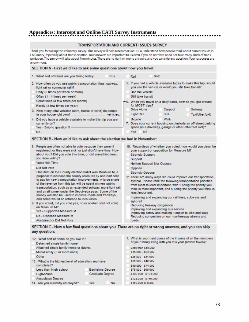
73
Appendices: Intercept and Online/CATI Survey Instruments
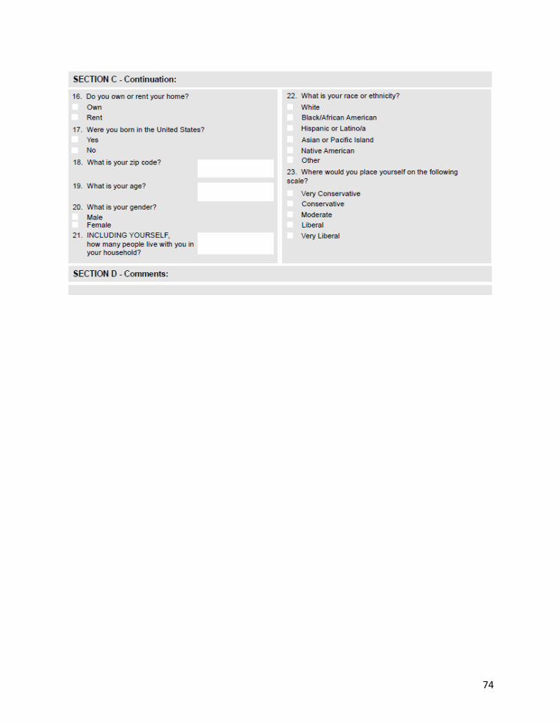
74
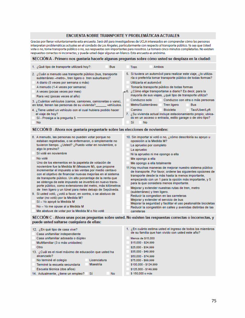
75
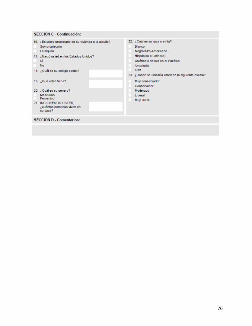
76
77
Online/CATI Survey Instrument
Question: qintro - 1 (Single)
Text:
Hi! My name is ______. I'm calling from a national research firm on behalf
of UCLA. This is a research study about current issues in Los Angeles
County. The study is being conducted by Michael Manville, Assistant
Professor in the Department of Urban Planning at UCLA. This study is only
for research purposes. It will help researchers understand how people like
you think about issues facing Los Angeles County. Your participation is
entirely voluntary. As part of this study you will answer questions about
current events facing Los Angeles County and provide some background
information about yourself. The study should take about 10-12 minutes.
There may be no direct benefit to you from participating in this study.
There is no more risk than would be expected from everyday typical
experiences. You may discontinue this study at any time, by hanging up.
The data we collect will be confidential, and we will not collect or
retain any information that would let you be identified by your answers.
You may refuse to answer any questions that you do not want to answer and
still remain in the study. If you should have any questions about this
research study, please contact UCLA researcher Mike Manville at (310) 825-
4025. If you have concerns about your rights while taking part in this
survey, or you have concerns or suggestions and want to talk to someone
other than the researchers about the study, please call the UCLA Office of
Human Subjects Research Protection Program at (310) 825-7122.
(qintro:1) Continue
(qintro:2) Callback/Not Available
(qintro:3) Refused
-------------------------------------------------------------------------
Question: q1 - 1 (Single)
Text:
Overall, do you think LA County is heading in the right direction?
(q1:1) Yes
(q1:2) No
(q1:3) Don't Know / Refused
-------------------------------------------------------------------------
Question: q49 - 1 (Single)
Text:
Record Gender by Observation.
(q49:1)Female
78
(q49:2)Male
(q49:4)Don't Know / refused
-------------------------------------------------------------------------
Question: q50 - 1 (Single)
Text:
What is your age?
(q50:1)18 to 24
(q50:2)25 to 34
(q50:3)35 to 44
(q50:4)45 to 54
(q50:5)55 to 64
(q50:6)65 to 74
(q50:7)75 or older
(q50:8)Don't Know / Refused
-------------------------------------------------------------------------
Question: q51 - 1 (Single)
Text:
What is your race or ethnicity?
(q51:1)White
(q51:2)Hispanic or Latino/a
(q51:3)Asian or Pacific Island
(q51:4)Native American
(q51:5)Other
(q51:6)Black/African-American
(q51:7)Prefer not to answer
-------------------------------------------------------------------------
Question: q52 - 2 (Single)
Text:
What is your best guess of the income of all members of your family living
with you this year (before taxes)?
(q52:01)Less than $15,000
(q52:02)$15,000 - $24,999
(q52:03)$25,000 to $34,999
(q52:04)$35,000 to $49,999
(q52:05)$50,000 to $74,999
(q52:06)$75,000 to $99,999
(q52:07)$100,000 to $124,999
(q52:08)$125,000 to $149,999
(q52:09)$150,000 or more
79
(q52:10)Don't Know / Refused
-------------------------------------------------------------------------
Question: q53 - 1 (Single)
Text:
What is the highest level of education you have completed?
(q53:1)Up to grade 12, no high school diploma
(q53:2)Graduated high school
(q53:3)Trade/technical school
(q53:4)Some college, no degree
(q53:5)Associate's degree
(q53:6)Bachelor's degree
(q53:7)Advanced degree (Master's, Ph.D., M.D.)
(q53:8)Don't Know / Refused
-------------------------------------------------------------------------
Question: q2_1 - 50 (Open-end)
Text:
What do you think are the two biggest challenges facing LA County right
now? - Option 1:
-------------------------------------------------------------------------
Question: q2_2 - 50 (Open-end)
Text:
What do you think are the two biggest challenges facing LA County right
now? - Option 2:
-------------------------------------------------------------------------
Question: q3 - 5 (Numeric)
Text:
LA County is big, and people across the County often have different
concerns and ideas. What is your zip code?
-------------------------------------------------------------------------
Question: q4 - 1 (Single)
Text:
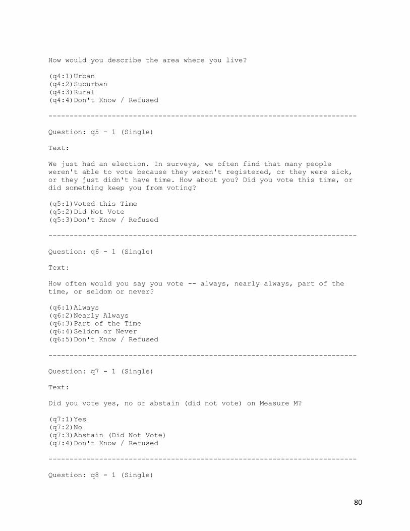
80
How would you describe the area where you live?
(q4:1)Urban
(q4:2)Suburban
(q4:3)Rural
(q4:4)Don't Know / Refused
-------------------------------------------------------------------------
Question: q5 - 1 (Single)
Text:
We just had an election. In surveys, we often find that many people
weren't able to vote because they weren't registered, or they were sick,
or they just didn't have time. How about you? Did you vote this time, or
did something keep you from voting?
(q5:1)Voted this Time
(q5:2)Did Not Vote
(q5:3)Don't Know / Refused
-------------------------------------------------------------------------
Question: q6 - 1 (Single)
Text:
How often would you say you vote -- always, nearly always, part of the
time, or seldom or never?
(q6:1)Always
(q6:2)Nearly Always
(q6:3)Part of the Time
(q6:4)Seldom or Never
(q6:5)Don't Know / Refused
-------------------------------------------------------------------------
Question: q7 - 1 (Single)
Text:
Did you vote yes, no or abstain (did not vote) on Measure M?
(q7:1)Yes
(q7:2)No
(q7:3)Abstain (Did Not Vote)
(q7:4)Don't Know / Refused
-------------------------------------------------------------------------
Question: q8 - 1 (Single)
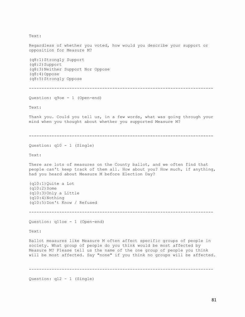
81
Text:
Regardless of whether you voted, how would you describe your support or
opposition for Measure M?
(q8:1)Strongly Support
(q8:2)Support
(q8:3)Neither Support Nor Oppose
(q8:4)Oppose
(q8:5)Strongly Oppose
-------------------------------------------------------------------------
Question: q9oe - 1 (Open-end)
Text:
Thank you. Could you tell us, in a few words, what was going through your
mind when you thought about whether you supported Measure M?
-------------------------------------------------------------------------
Question: q10 - 1 (Single)
Text:
There are lots of measures on the County ballot, and we often find that
people can't keep track of them all. How about you? How much, if anything,
had you heard about Measure M before Election Day?
(q10:1)Quite a Lot
(q10:2)Some
(q10:3)Only a Little
(q10:4)Nothing
(q10:5)Don't Know / Refused
-------------------------------------------------------------------------
Question: q11oe - 1 (Open-end)
Text:
Ballot measures like Measure M often affect specific groups of people in
society. What group of people do you think would be most affected by
Measure M? Please tell us the name of the one group of people you think
will be most affected. Say "none" if you think no groups will be affected.
-------------------------------------------------------------------------
Question: q12 - 1 (Single)
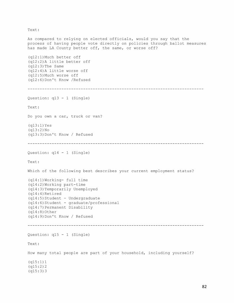
82
Text:
As compared to relying on elected officials, would you say that the
process of having people vote directly on policies through ballot measures
has made LA County better off, the same, or worse off?
(q12:1)Much better off
(q12:2)A little better off
(q12:3)The Same
(q12:4)A little worse off
(q12:5)Much worse off
(q12:6)Don't Know /Refused
-------------------------------------------------------------------------
Question: q13 - 1 (Single)
Text:
Do you own a car, truck or van?
(q13:1)Yes
(q13:2)No
(q13:3)Don't Know / Refused
-------------------------------------------------------------------------
Question: q14 - 1 (Single)
Text:
Which of the following best describes your current employment status?
(q14:1)Working- full time
(q14:2)Working part-time
(q14:3)Temporarily Unemployed
(q14:4)Retired
(q14:5)Student - Undergraduate
(q14:6)Student - graduate/professional
(q14:7)Permanent Disability
(q14:8)Other
(q14:9)Don't Know / Refused
-------------------------------------------------------------------------
Question: q15 - 1 (Single)
Text:
How many total people are part of your household, including yourself?
(q15:1)1
(q15:2)2
(q15:3)3
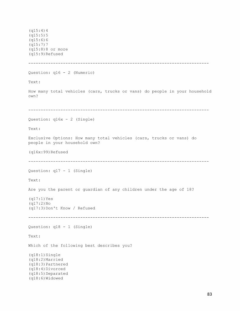
83
(q15:4)4
(q15:5)5
(q15:6)6
(q15:7)7
(q15:8)8 or more
(q15:9)Refused
-------------------------------------------------------------------------
Question: q16 - 2 (Numeric)
Text:
How many total vehicles (cars, trucks or vans) do people in your household
own?
-------------------------------------------------------------------------
Question: q16x - 2 (Single)
Text:
Exclusive Options: How many total vehicles (cars, trucks or vans) do
people in your household own?
(q16x:99)Refused
-------------------------------------------------------------------------
Question: q17 - 1 (Single)
Text:
Are you the parent or guardian of any children under the age of 18?
(q17:1)Yes
(q17:2)No
(q17:3)Don't Know / Refused
-------------------------------------------------------------------------
Question: q18 - 1 (Single)
Text:
Which of the following best describes you?
(q18:1)Single
(q18:2)Married
(q18:3)Partnered
(q18:4)Divorced
(q18:5)Separated
(q18:6)Widowed
84
(q18:7)Other
(q18:8)Refused
-------------------------------------------------------------------------
Question: q19 - 2 (Single)
Text:
What is your primary way of getting to work on most work days? In other
words, on a typical day, how do you travel for most of your commute?
(q19:01)Drive Alone
(q19:02)Carpool
(q19:03)Subway
(q19:04)Light Rail
(q19:05)Bus
(q19:06)Bicycle
(q19:07)Taxi/ Uber/Lyft
(q19:08)Walk
(q19:09)Work at Home
(q19:10)Commuter Rail
(q19:11)Other
(q19:12)Don't know / refused
-------------------------------------------------------------------------
Question: q20 - 2 (Single)
Text:
When you travel on a daily basis for purposes other than commuting to and
from work, how do you get around for most trips?
(q20:01)Drive Alone
(q20:02)Carpool
(q20:03)Subway
(q20:04)Light Rail
(q20:05)Bus
(q20:06)Bicycle
(q20:07)Taxi/Uber/Lyft
(q20:08)Walk
(q20:09)Other
(q20:10)Don't Know / Refused
-------------------------------------------------------------------------
Question: q21 - 1 (Single)
Text:
When you travel on a daily basis, how do you get around for MOST trips?
(q21:1)Drive Alone
85
(q21:2)Carpool
(q21:3)Subway
(q21:4)Light Rail
(q21:5)Bus
(q21:6)Taxi/Uber/Lyft
(q21:7)Bicycle
(q21:8)Walk
(q21:9)Don't Know / Refused
-------------------------------------------------------------------------
Question: q22 - 1 (Single)
Text:
How often do you ride a bicycle?
(q22:1)Often (more than three times a week)
(q22:2)Sometimes (1-3 times per week)
(q22:3)Rarely (a few times per month)
(q22:4)Almost never (a few times per year or less)
(q22:5)Don't Know / Refused
-------------------------------------------------------------------------
Question: q23 - 3 (Numeric)
Text:
In minutes, how long would it take you to walk to the public
transportation stop closest to your home? If you don't know, respond with
'don't know'.
-------------------------------------------------------------------------
Question: q23x - 4 (Single)
Text:
Exclusive Options: In minutes, how long would it take you to walk to the
public transportation stop closest to your home? If you don't know,
respond with 'don't know'.
(q23x:9999)Don't know
-------------------------------------------------------------------------
Question: q24 - 1 (Single)
Text:
How often do you use public transportation (bus, subway, light rail or
commuter rail)?
86
(q24:1)Often (once a week or more)
(q24:2)Sometimes (a few times a month)
(q24:3)Rarely (a few times a year)
(q24:4)I never use public transportation
(q24:5)Don't Know / Refused
-------------------------------------------------------------------------
Question: q25 - 1 (Single)
Text:
What sort of home do you live in?
(q25:1)Detached single family home
(q25:2)Attached single family home or duplex
(q25:3)Multi-Family (3 or more units)
(q25:4)Other
(q25:5)Don't Know / Refused
-------------------------------------------------------------------------
Question: q26 - 1 (Single)
Text:
Do you own or rent your home?
(q26:1)Own
(q26:2)Rent
(q26:3)Don't Know / Refused
-------------------------------------------------------------------------
Question: q27 - 1 (Single)
Text:
Does your current housing unit include an off-street parking space (in a
driveway, garage or other off-street slot)?
(q27:1)Yes
(q27:2)No
(q27:3)Don't Know / Refused
-------------------------------------------------------------------------
Question: q28 - 1 (Single)
Text:
Does your workplace provide free parking if you drive to work?
87
(q28:1)Yes
(q28:2)No
(q28:3)Don't Know / Refused
-------------------------------------------------------------------------
Question: q29 - 1 (Single)
Text:
How often does traffic congestion on the road slow down your daily travel?
(q29:1)Never
(q29:2)Once a week
(q29:3)Two or three times a week
(q29:4)Every day
(q29:5)Don't Know / Refused
-------------------------------------------------------------------------
Question: q30 - 1 (Single)
Text:
Now for a slightly different topic. Housing development is always a big
issue in Los Angeles County. On election day, some cities in LA County
voted on proposals to restrict new housing development, and especially to
restrict the density of housing in their cities. In general, do you
support or oppose building more housing, and increasing housing density,
in Los Angeles County?
(q30:1)Strongly support
(q30:2)Support
(q30:3)Neither Support Nor Oppose
(q30:4)Oppose
(q30:5)Strongly Oppose
(q30:6)Don't know / refused
-------------------------------------------------------------------------
Question: q31 - 1 (Single)
Text:
Do you support or oppose building more housing in your own neighborhood?
(q31:1)Strongly Support
(q31:2)Support
(q31:3)Neither Support Nor Oppose
(q31:4)Oppose
(q31:5)Strongly Oppose
(q31:6)Don't Know / Refused
-------------------------------------------------------------------------
88
Question: q32 - 1 (Single)
Text:
Still thinking about housing development, please tell us how much you
agree or disagree with the following statements. - New housing development
will make housing more affordable throughout LA County.
(q32:1)Strongly Agree
(q32:2)Agree
(q32:3)Neither Agree Nor Disagree
(q32:4)Disagree
(q32:5)Strongly Disagree
-------------------------------------------------------------------------
Question: q33 - 1 (Single)
Text:
Still thinking about housing development, please tell us how much you
agree or disagree with the following statements. - New housing development
will bring more cars and make congestion worse.
(q33:1)Strongly Agree
(q33:2)Agree
(q33:3)Neither Agree Nor Disagree
(q33:4)Disagree
(q33:5)Strongly Disagree
-------------------------------------------------------------------------
Question: q34 - 1 (Single)
Text:
Still thinking about housing development, please tell us how much you
agree or disagree with the following statements. - New housing development
will be expensive, and make housing less affordable.
(q34:1)Strongly Agree
(q34:2)Agree
(q34:3)Neither Agree Nor Disagree
(q34:4)Disagree
(q34:5)Strongly Disagree
-------------------------------------------------------------------------
Question: q35 - 1 (Single)
Text:
89
Still thinking about housing development, please tell us how much you
agree or disagree with the following statements. - New housing development
creates jobs, and helps LA County's economy.
(q35:1)Strongly Agree
(q35:2)Agree
(q35:3)Neither Agree Nor Disagree
(q35:4)Disagree
(q35:5)Strongly Disagree
-------------------------------------------------------------------------
Question: q36 - 1 (Single)
Text:
Still thinking about housing development, please tell us how much you
agree or disagree with the following statements. - New housing development
will make it easier for people to walk, bike and take public
transportation.
(q36:1)Strongly Agree
(q36:2)Agree
(q36:3)Neither Agree Nor Disagree
(q36:4)Disagree
(q36:5)Strongly Disagree
-------------------------------------------------------------------------
Question: q37 - 1 (Single)
Text:
Thinking about social problems like poverty, pollution and traffic
congestion, would you say that you generally believe the government has a
strong responsibility to step in and help solve these problems, or do you
generally believe problems like these will be solved when individuals step
up and change their own behavior?
(q37:1)Government has a responsibility to help solve them
(q37:2)Individuals need to take responsibility and change their behavior
(q37:3)Don't Know / Refused
-------------------------------------------------------------------------
Question: q38_1 - 1 (Numeric)
Text:
Let's switch back to transportation for a moment. Transportation is always
a big issue in LA County, and there are many ways we could improve our
transportation system. Please rank the following transportation priorities
from most to least important, with 1 being the priority you think is most
90
important, and 5 being the priority you think is least important. -
Improving and expanding our subways, light rail lines, and commuter trains
-------------------------------------------------------------------------
Question: q38_2 - 1 (Numeric)
Text:
Let's switch back to transportation for a moment. Transportation is always
a big issue in LA County, and there are many ways we could improve our
transportation system. Please rank the following transportation priorities
from most to least important, with 1 being the priority you think is most
important, and 5 being the priority you think is least important. -
Reducing freeway congestion, and making travel on our freeways faster
-------------------------------------------------------------------------
Question: q38_3 - 1 (Numeric)
Text:
Let's switch back to transportation for a moment. Transportation is always
a big issue in LA County, and there are many ways we could improve our
transportation system. Please rank the following transportation priorities
from most to least important, with 1 being the priority you think is most
important, and 5 being the priority you think is least important. -
Improving and expanding our bus service
-------------------------------------------------------------------------
Question: q38_4 - 1 (Numeric)
Text:
Let's switch back to transportation for a moment. Transportation is always
a big issue in LA County, and there are many ways we could improve our
transportation system. Please rank the following transportation priorities
from most to least important, with 1 being the priority you think is most
important, and 5 being the priority you think is least important. -
Adding bicycle lanes, and improving safety for biking and walking
-------------------------------------------------------------------------
Question: q38_5 - 1 (Numeric)
Text:
Let's switch back to transportation for a moment. Transportation is always
a big issue in LA County, and there are many ways we could improve our
91
transportation system. Please rank the following transportation priorities
from most to least important, with 1 being the priority you think is most
important, and 5 being the priority you think is least important. -
Improving traffic flow and reducing congestion on our streets and roads
-------------------------------------------------------------------------
Question: q39 - 1 (Single)
Text:
One issue that always gets a lot of attention is parking. Currently, when
developers build housing in LA County, cities require them to include
parking spaces for residents and visitors. These parking requirements can
be controversial, and some cities might remove them. Thinking about these
parking requirements, please tell us how much you agree or disagree with
the following statements: - Requiring developers to build parking reduces
the impact of development on the surrounding neighborhood.
(q39:1)Strongly Agree
(q39:2)Agree
(q39:3)Neither Agree nor Disagree
(q39:4)Disagree
(q39:5)Strongly Disagree
-------------------------------------------------------------------------
Question: q40 - 1 (Single)
Text:
One issue that always gets a lot of attention is parking. Currently, when
developers build housing in LA County, cities require them to include
parking spaces for residents and visitors. These parking requirements can
be controversial, and some cities might remove them. Thinking about these
parking requirements, please tell us how much you agree or disagree with
the following statements: - Requiring developers to build parking will
make people drive more.
(q40:1)Strongly Agree
(q40:2)Agree
(q40:3)Neither Agree nor Disagree
(q40:4)Disagree
(q40:5)Strongly Disagree
-------------------------------------------------------------------------
Question: q41 - 1 (Single)
Text:
One issue that always gets a lot of attention is parking. Currently, when
developers build housing in LA County, cities require them to include
92
parking spaces for residents and visitors. These parking requirements can
be controversial, and some cities might remove them. Thinking about these
parking requirements, please tell us how much you agree or disagree with
the following statements: - Requiring developers to build parking makes it
harder to build housing, and makes housing more expensive.
(q41:1)Strongly Agree
(q41:2)Agree
(q41:3)Neither Agree nor Disagree
(q41:4)Disagree
(q41:5)Strongly Disagree
-------------------------------------------------------------------------
Question: q42 - 1 (Single)
Text:
One issue that always gets a lot of attention is parking. Currently, when
developers build housing in LA County, cities require them to include
parking spaces for residents and visitors. These parking requirements can
be controversial, and some cities might remove them. Thinking about these
parking requirements, please tell us how much you agree or disagree with
the following statements: - Housing close to public transit should not be
required to include as much parking, because residents are less likely to
own cars.
(q42:1)Strongly Agree
(q42:2)Agree
(q42:3)Neither Agree nor Disagree
(q42:4)Disagree
(q42:5)Strongly Disagree
-------------------------------------------------------------------------
Question: q43_1 - 1 (Numeric)
Text:
Now we have just a couple more questions about transportation. Thinking
about public transportation in particular, people have different reasons
for wanting to expand LA County's public transit system. Regardless of
whether you support or oppose Measure M, which of the following do you
think are the best reasons to invest more in public transportation? Please
rank the reasons below, with 1 being the reason you think is most
important, and 4 being the reason you think is least important. - We
need to reduce traffic congestion on our roads
-------------------------------------------------------------------------
Question: q43_2 - 1 (Numeric)
Text:
93
Now we have just a couple more questions about transportation. Thinking
about public transportation in particular, people have different reasons
for wanting to expand LA County's public transit system. Regardless of
whether you support or oppose Measure M, which of the following do you
think are the best reasons to invest more in public transportation? Please
rank the reasons below, with 1 being the reason you think is most
important, and 4 being the reason you think is least important. - We
need to reduce air pollution and global warming
-------------------------------------------------------------------------
Question: q43_3 - 1 (Numeric)
Text:
Now we have just a couple more questions about transportation. Thinking
about public transportation in particular, people have different reasons
for wanting to expand LA County's public transit system. Regardless of
whether you support or oppose Measure M, which of the following do you
think are the best reasons to invest more in public transportation? Please
rank the reasons below, with 1 being the reason you think is most
important, and 4 being the reason you think is least important. - We
need to help lower-income people who depend on transit
-------------------------------------------------------------------------
Question: q43_4 - 1 (Numeric)
Text:
Now we have just a couple more questions about transportation. Thinking
about public transportation in particular, people have different reasons
for wanting to expand LA County's public transit system. Regardless of
whether you support or oppose Measure M, which of the following do you
think are the best reasons to invest more in public transportation? Please
rank the reasons below, with 1 being the reason you think is most
important, and 4 being the reason you think is least important. - We
need to create construction jobs from building new transit lines
-------------------------------------------------------------------------
Question: q44 - 1 (Single)
Text:
Some transportation officials argue that the best solution to LA County's
traffic congestion is to make driving more expensive at busy times. For
example, if we had tolls on our freeways that were higher when many people
wanted to drive, such as at rush hour, congestion would go down. Would
you support or oppose using tolls like this on LA County's freeways?
94
(q44:1)Strongly Support
(q44:2)Support
(q44:3)Neither Support Nor Oppose
(q44:4)Oppose
(q44:5)Strongly Oppose
-------------------------------------------------------------------------
Question: q45 - 1 (Single)
Text:
Still thinking about transportation, please tell us how much you agree or
disagree with the following statements. - My community would benefit from
more public transportation options.
(q45:1)Strongly Agree
(q45:2)Agree
(q45:3)Neither Agree Nor Disagree
(q45:4)Disagree
(q45:5)Strongly Disagree
-------------------------------------------------------------------------
Question: q46 - 1 (Single)
Text:
Still thinking about transportation, please tell us how much you agree or
disagree with the following statements. - I would like to drive less.
(q46:1)Strongly Agree
(q46:2)Agree
(q46:3)Neither Agree Nor Disagree
(q46:4)Disagree
(q46:5)Strongly Disagree
-------------------------------------------------------------------------
Question: q47 - 1 (Single)
Text:
Still thinking about transportation, please tell us how much you agree or
disagree with the following statements. - My life and daily routine would
change for the better if public transportation were faster and more
convenient.
(q47:1)Strongly Agree
(q47:2)Agree
(q47:3)Neither Agree Nor Disagree
(q47:4)Disagree
(q47:5)Strongly Disagree
95
-------------------------------------------------------------------------
Question: q48 - 1 (Single)
Text:
Still thinking about transportation, please tell us how much you agree or
disagree with the following statements. - My life and daily routine would
change for the better if our freeways and roads were less congested.
(q48:1)Strongly Agree
(q48:2)Agree
(q48:3)Neither Agree Nor Disagree
(q48:4)Disagree
(q48:5)Strongly Disagree
-------------------------------------------------------------------------
Question: q54 - 1 (Single)
Text:
Were you born in the United States?
(q54:1)Yes
(q54:2)No
(q54:3)Don't Know / Refused
-------------------------------------------------------------------------
Question: q55 - 1 (Single)
Text:
Generally speaking, do you think of yourself as a Republican, a Democrat,
an Independent, or what?
(q55:1)Republican
(q55:2)Democrat
(q55:3)Independent
(q55:4)Other
(q55:5)Don't Know / Refused
-------------------------------------------------------------------------
Question: q56 - 1 (Single)
Text:
Would you call yourself a strong Republican or a not very strong
Republican?
(q56:1)Strong Republican
96
(q56:2)Not Very Strong Republican
(q56:3)Don't Know / Refused
-------------------------------------------------------------------------
Question: q57 - 1 (Single)
Text:
Would you call yourself a strong Democrat or a not very strong Democrat?
(q57:1)Strong Democrat
(q57:2)Not Very Strong Democrat
(q57:3)Don't Know / Refused
-------------------------------------------------------------------------
Question: q58 - 1 (Single)
Text:
Do you think of yourself as closer to the Republican Party or to the
Democratic Party?
(q58:1)Republican
(q58:2)Democrat
(q58:3)Don't Know / Refused
-------------------------------------------------------------------------
Question: q59 - 1 (Single)
Text:
Where would you place yourself on the following scale?
(q59:1)Very Conservative
(q59:2)Conservative
(q59:3)Moderate
(q59:4)Liberal
(q59:5)Very Liberal
(q59:6)Don't Know / Refused