Measurement of Calibrated Recursive Analytic in the …...• Gas Tungsten Arc Welding (GTAW) • Analytic Model • Weld Penetration • Weld Pool • Three-Dimensional Vision (3D)

WELDING RESEARCH

WELDING JOURNAL / APRIL 2018, VOL. 97108-s

https://doi.org/10.29391/2018.97.010

Introduction

This work is a continuation of our recent efforts (Refs. 1,2) to establish the scientific foundation for monitoring howdeeply a developing weld pool has penetrated underneaththe workpiece during gas tungsten arc welding (GTAW).Since the depth of the weld pool is not directly measurable,various techniques, including vision sensing (Refs. 3–7),pool oscillation (Refs. 8–11), ultrasound (Refs. 12–16), andinfrared (Refs. 17–19) have been proposed to obtain indirect

measurements. Efforts have been taken to interpret themby characterizing the weld pool surface (such as width,length, and convexity) from vision sensing (Refs. 20–22),analyzing process parameters (such as current, voltage, andspeed) (Refs. 23–26), or modeling human welder responsesto the dynamic weld pool surface (Refs. 27–30) to bettercorrelate the measurements to the penetration of the weldpool. Analytic models have also been proposed to controlthe penetration as calibrated by online measurements (Ref.31), but the relation between the measurements and the an-alytic model parameters is empirical. In our recent efforts (Refs. 1, 2), a different approach was

taken with the hope that the penetration and measurementsmay be better correlated based on a more solid scientificfoundation. This approach used an analytic model to com-pute the temperature distribution and then calibrated it us-ing measured weld pool surface. To this end, Nguyen’s sin-gle-ellipsoidal stationary, heat-source based analytic solu-tion (Ref. 32) was used to provide an initial temperature dis-tribution in the workpiece. The computed weld pool radiusstationary welding was compared with that from the meas-urement. The temperature distribution was then shrunk/ex-panded through an adjustment ratio in the radius direction(x-y directions) such that the error of the computed radiuswith the measurement became zero. The calibrated tempera-ture distribution was then used to compute the increase inthe volume due to thermal expansion. The resultant volumewas then compared with that from the measurement on theweld pool surface. The temperature distribution wasshrunk/expanded again but in the depth direction such thatthe volume error also became zero. The temperature distri-bution was thus fully calibrated in all directions. The above-mentioned analytic model was developed, cali-brated, and verified under a given constant current and auniform preheating temperature. Its ability to predict thepenetration depth accurately has been verified through com-parison with the measured cross sections of welds. Whilethis calibrated analytic model may predict the penetrationdepth and be used to produce the desirable penetrationdepth, developing the weld pool including weld width andpenetration in desirable ways within the desired time re-

Measurement of Calibrated Recursive Analyticin the Gas Tungsten Arc Weld Pool Model

Temperature distribution is correlated to its history and newly applied arc energy

BY S. J. WU, H. M. GAO, W. ZHANG, AND Y. M. ZHANG

ABSTRACT

An analytic model based on a single-ellipsoidal stationaryheat source can estimate the penetration in gas tungsten arcwelding (GTAW) accurately with the calibration from the 3Dmeasurements of the weld pool surface. However, the com-putation needed for the integration associated with the ana-lytic model increases with time and when the current ischanged; its real-time application is no longer feasible. To ad-dress this challenge, the basic principles on which theanalytic model was derived were analyzed to rebuild a modi-fied analytic model. In this rebuilt model, the temperature dis-tribution was expressed into two terms: one as a function ofan earlier temperature distribution, and the other as afunction of the newly applied arc power. With this rebuilt ana-lytic model, a recursive solution was facilitated such that thecomputation does not increase/change as the welding timeincreases and the desirable real-time computation and cali-bration can be obtained. To further reduce the computationtime, a model was fit for the earlier distribution as given bydiscrete points such that its function can be analyticallyevaluated to minimize the needed online computation. Experi-ments were performed where cross sections of the weldswere used to verify the novel recursive model calibrated bythe measurements of the 3D weld pool surface.

KEYWORDS • Gas Tungsten Arc Welding (GTAW) • Analytic Model • Weld Penetration • Weld Pool • Three-Dimensional Vision (3D)

Wu/Zhang Supplementcorr.qxp_Layout 1 3/7/18 3:27 PM Page 108

WELDING RESEARCH

APRIL 2018 / WELDING JOURNAL 109-s

quires real-time adjustments on the arc power/current. Ana-lytic models thus need to derive for a varying current, andthis work is devoted to addressing this issue as a continua-tion of our recent efforts in using analytic computation andcalibration methods to correlate measurements to weld pen-etration based on a solid scientific foundation. Using the analytic model, the temperature distribution attf > 0 can be computed as an integral from the initial time tothe current time tf. Since the function to be integratedchanges with tf, the integration over the entire time period[0, tf] is computed each time as the time tf changes/goes. In-tegrations/computations in different times are not correlat-ed and the computation for the integration increased withthe time. For a given constant current, all the computationsmay be performed offline in advance and the computedtemperature distributions at different times are stored.However, when the current varies, computing and storingtemperature distributions in advance is no longer feasible. To address the challenge from the continuously increas-ing computation, the authors wondered if the temperaturedistribution may be analytically correlated to an earlier dis-tribution and newly applied current. With such a correla-tion, a recursive solution may be facilitated such that thecomputation does not increase or change with the time. Notonly can large storage be avoided, but also real-time compu-tation and calibration can be obtained. Obtaining this needed analytic correlation is challengingbecause the previous methods used for derivations are not ful-ly and directly applicable, in particular the constant currentand initial temperature field. To address this challenge, the au-thors first analyzed the basic principles that the previous deri-vations were based on and applied them to the new conditionsto derive an analytic model that works under varying current.Then the analytic model, also as an integration over time, wasdecomposed into integrations in two different time intervals.Further analysis led to the favorable result that they are sepa-rately determined by an earlier temperature distribution histo-ry and the newly applied arc energy. More excitingly, the authors analyzed the two terms andfound they are the spatial convolution of the earlier tempera-ture distribution with the heat source distribution and themultiplication of a fixed integration with the newly appliedcurrent (arc energy). While the fixed integration can be com-puted in advance, the spatial convolution cannot because the

earlier temperature distribution varies. Numerical evaluationof the convolution is still computationally intensive. To obtainan analytic solution for the convolution, the earlier tempera-ture distribution is used to fit an analytic description. Withthe analytic description for the earlier temperature distribu-tion, its convolution with the heat source distribution, givenanalytically, can be analytically solved to minimize the neededcomputation. This paper is organized as follows. In the “Analytic Mod-el” section, the analytic model for varying current is derived.The “Experimental Procedure” section describes the obser-vation system and experimental conditions. The calibratedpenetration and its experimental identification are shown inthe “Verification and Analysis” section. And, finally, conclu-sions are drawn in the “Conclusions” section.

Analytic Model

The analytic model to compute the temperature distribu-tion evolution T(x,y,z)t tf (the temperature distribution attime tf) for a point heat source is derived by Rosenthal (Ref.33). This derivation is enabled through the following ap-proximations/principles: 1) plate thickness being infinite; 2)heat transfer being conductive; 3) initial temperature beinguniform; and 4) effects of the continuous heat applied at thedifferent times being summable through the superpositionprinciple. The derivation starts with applying the superposi-tion principle to obtain the temperature distributionG(x,y,z)t as the unit response of the heat source is continu-ously applied in [0, t]:

G x,y,z( )t = 0

t�

1

4�a t��( )( )3/2�c�exp x

2 + y2 + z2

4a t��( ) d�

= 1�c

��

�� 0

t�

1

4�a t��( )( )3/2 �expx2 + y2 + z2

4a t� �( ) d�

= 1�c

��

��

g x ,y,z( )t��0

t� d� 1( )

Fig. 1 — Sketch of Goldak’s body heat source (Ref. 34). Fig. 2 — Monitoring of the weld pool surface using a low-power illumination laser.


WELDING RESEARCH

WELDING JOURNAL / APRIL 2018, VOL. 97110-s

where g(x,y,z)t = 1/(4at)3/2 exp [x2+y2+z2/]4at; a is the ther-mal diffusivity a k/c; and c are the density and specificheat, respectively; k is the thermal conductivity; and is thetime of heat source application. Despite the use of all thesearguable assumptions, Rosenthal’s derivation and the result-ant analytic solution have been widely accepted by the weld-ing community although its actual applicability is still sub-ject to verification for the specific applications. Further, for distributive heat source, the analytic solutionhas been enabled by the use of a single-ellipsoidal static heatsource

proposed by Goldak (Ref. 34) as illustrated in Fig. 1, where isthe effective heat-input coefficient that is chosen as 100% inthis study because the results will be calibrated after calcula-tion; V and I are welding voltage and welding current, respec-tively; and ah, bh, ch, are the single-ellipsoidal heat source pa-rameters. The temperature distribution under a distributive heatsource can be obtained by convoluting the point heat sourcesolution (Equation 1) with the heat distribution (Equation 2)to superposition spatially. After simplification, the followinganalytic solution for the temperature distribution can be ob-tained (Ref. 35):

T(x,y,z)t tf S(x,y,z) G(x,y,z)tf

where P V I is the power of the effective heat inputfrom the arc and

Equation 3 is for the temperature distribution in theworkpiece from a uniform initial room temperature underthe application of a constant distributive power source.However, for real-time control applications, the authors tar-get at the current I () (thus P ()) is adjusted according tothe feedback form the in-situ penetration depth in real-time. Equation 3 is thus not, at least not directly, applicable.Hence, deriving an analytic model that can suit for a variedcurrent/arc power that changes its value at a discrete time isnecessary for future optimization of the welding process.

Analytic Model with Varied Current

The superposition principle has been applied in obtain-ing Equations 1 and 3. Since the superposition principle isindependent from the input and the spatial convolution isindependent of time, the following solution under the vary-ing current/arc power can be directly obtained:

To obtain the desirable recursive solution, consider tf tk

+ t the next time temperature distribution is computed. Assuch, the present time tk is t earlier than tf tk + t and wewish to correlate the temperature distribution at tf tk + tto its history (temperature distribution) at tk and the newlyapplied power Ptk during [(tk,tk + t)]. Hence, the followingderivation is made:

= 3 3P�c� �

�0

tf�1

12a tf ��( )+ah2 12a tf ��( )+bh2 12a tf ��( )+ ch2

�exp � 3x2

12a tf ��( )+ ch2� 3y2

12a tf ��( )+ah2� 3z2

12a tf ��( )+bh2�

�

� d�

=0

tf� P �fx ,y ,z tf ��( )d� 3( )

fx ,y ,z t��( )= 3 3

�c� � 12a t��( )+ah2 12a t��( )+bh2 12a t��( )+ ch2

�exp � 3x2

12a t��( )+ ch2� 3y2

12a t��( )+ah2� 3z2

12a t��( )+bh2�

��

�

��

S x ,y,z( )= 6 3�� V �Iahbhch� �

�exp �3x2

ch2 � 3y

2

ah2 � 3z

2

bh2

�

��

��2( )

T x ,y,z( )t=tf = P0

tf� �( )�fx ,y ,z tf � �( )d� 3A( )

Fig. 4 — Measured diameter and convexity of the weld poolsurface from the verification experiment.Fig. 3 — Welding current used in the verification experiment.


WELDING RESEARCH


where Ptk = Vtk Itk is the effective power of the arc in (tk,tk + t). Since the current is not adjusted between two sam-pling instants, the arc power in the time interval (tk ,tk + t)is constant, as determined by the control algorithm at thesampling time tk , and is thus denoted by subscript tk. To understand the implication of decomposition (4), let’sexamine the second term first:

where Bx,y,z 0t {fx,y,z(t-t)t}dt is a constant, when t is

fixed, for a given point (x,y, z) and Qtk is the newly applied

arc energy during (tk, tk + 1). To see the nature of the firstterm, let’s examine the spatial convolution of the earliertemperature distribution T(x,y,z)tk and g(x,y,z)t:

By using the Gaussian integral, the above equation can besimplified as follows:

T(x,y,z)tk g(x,y,z)t

T x ,y,z( )tk+�t = P �( )�fx ,y ,z0

tk+�t

� tk +�t��( )d�

= P0

tk� �( )�fx ,y ,z tk +�t��( )d�

+ Ptktk

tk+�t� �fx ,y ,z tk +�t� �( )d�

= P0

tk� �( )�fx ,y ,z tk +�t��( )d�+ Ptk0

�t� �fx ,y ,z �t� �( )d� 4( )

Pt0

�t� k

�fx ,y ,z �t� �( )d�= Ptk�t{ } fx ,y ,z �t��( ) / �t{ }0

�t� d�

= Bx ,y ,zQtk 5( )

T x ,y,z( )tk � g x ,y,z( )�t = Q �( )�fx ,y ,z tk � �( )d�0

tk

��

��

��

�

1

4�a�t( )3/2 �expx2 + y2 + z2

4a�t

��

��

��

�

=3 3Q �( )

�c� � 12a tk ��( )+ah2 12a tk ��( )+bh2 12a tk ��( )+ ch2��+��0

tk�

�exp � 3u2

12a tk � �( )+ ch2� 3v2

12a tk � �( )+ah2� 3w2

12a tk � �( )+bh2�

��

�

��

� 1

4�a�t( )3/2 �exp �x�u( )2 + y� v( )2 + z�w( )2

4a�t

�

��

�

�� dudvdwd�

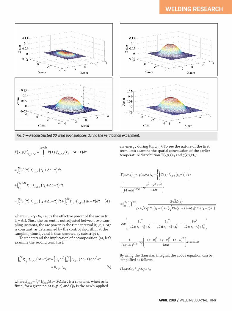
Fig. 5 — Reconstructed 3D weld pool surfaces during the verification experiment.


WELDING RESEARCH

WELDING JOURNAL / APRIL 2018, VOL.97112-s

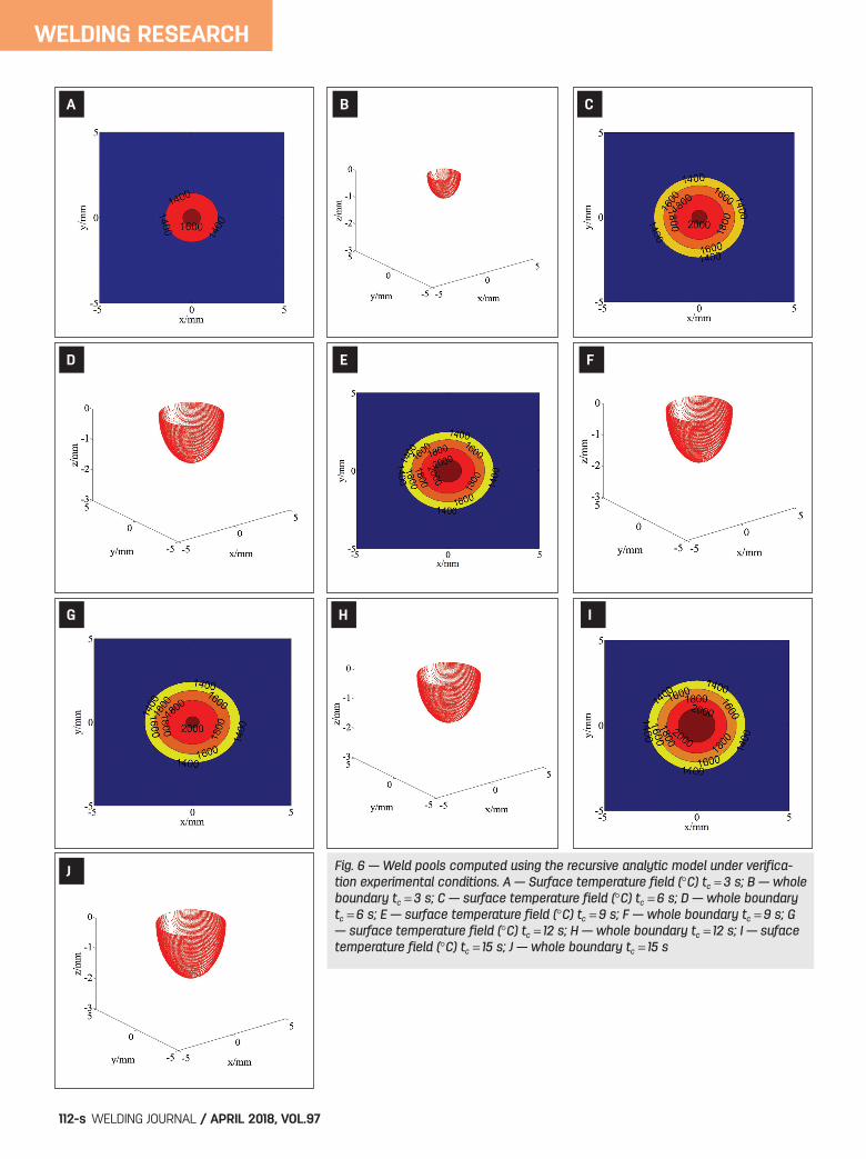
Fig. 6 — Weld pools computed using the recursive analytic model under verifica-tion experimental conditions. A — Surface temperature field (C) tc 3 s; B — wholeboundary tc 3 s; C — surface temperature field (C) tc 6 s; D — whole boundarytc 6 s; E — surface temperature field (C) tc 9 s; F — whole boundary tc 9 s; G— surface temperature field (C) tc 12 s; H — whole boundary tc 12 s; I — sufacetemperature field (C) tc 15 s; J — whole boundary tc 15 s

A B C

D E F

G

J

H I


WELDING RESEARCH


As such, another term is indeed the contribution fromthe earlier temperature distribution T(x,y,z) through its spa-tial convolution with g(x,y,z)t. Since g(x,y,z)t is a givenfunction of (x,y,z) when t is fixed, A is a given function ofthe temperature history T(x,y,z)tk. Hence,

T(x,y,z)tk1 A(T(x,y,z)tk) Bx,y,zQtk (7)

with the first term as a function of the earlier temperaturedistribution and second term as a function of newly appliedarc energy. Both functions also depend on t used, butwould only be (x,y,z) dependent when t is fixed.

Computation

While the computation for Bx,y,z 0t {fx,y,z(t - t)t}dt us-

ing a numerical method is straightforward and can be comput-

ed for each (x,y,z) of interest in advance, the computation ofA(T(x,y,z)tk) requires the knowledge of the varying T(x,y,z)tk,which is not available in advance. As a result, A(T(x,y,z)tk) mustbe computed in real-time each time. This is a challenging taskbecause A(T(x,y,z)tk) must be computed as the convolution ofthe calibrated T(x,y,z)tk), rather than the previously computedg(x,y,z)t, and the calibrated T(x,y,z)tk) will be given as a largeset of data at discrete points. Computing the three-dimension-al spatial convolution using a numerical computation is notfeasible for real-time applications. To overcome this difficulty, one may consider fittingT(x,y,z)tk into an analytic description whose convolution canbe solved analytically. To this end, the following descriptionis proposed for the temperature distribution:

where Ttop is an adjustable scale and (Kk1, Kk2, Kk3) are theshape parameters. This description is proposed because Ttop

can represent the peak temperature at the arc, and the de-creases in the temperature away from the center in the dif-ferent directions can be described similarly as the heatsource distribution. For identification purpose, this nonlin-ear model may be easily transformed into a linear equation

such that the linear least square estimate of (Ln(Ttop),- 1/K2

k1 - 1/K2k2, - 1/K2

k3)T can be obtained analytically to

=3 3Q �( )�c� �0

tk

�

� 1

12a tk+�t��( )+ah2 12a t

k+�t��( )+bh2 12a t

k+�t��( )+ ch2

�exp � 3x2

12a tk+�t��( )+ ch2 � 3y2

12a tk+�t��( )+ ah

2 � 3z2

12a tk+�t��( )+bh2

��

�

��d�

= Q �( )0

tk� �fx ,y ,z tk +�t��( )d� = A T x ,y,z( )tk( ) 6( )

T x ,y,z( )tk =Ttop �exp � x2

Kk1

2 � y2

Kk2

2 � z2

Kk23

�

��

�

�� 8( )

Ln T x ,y,z( )tk( )= Ln Ttop( )� x2

Kk1

2 � y2

Kk2

2 � z2

Kk32 9( )

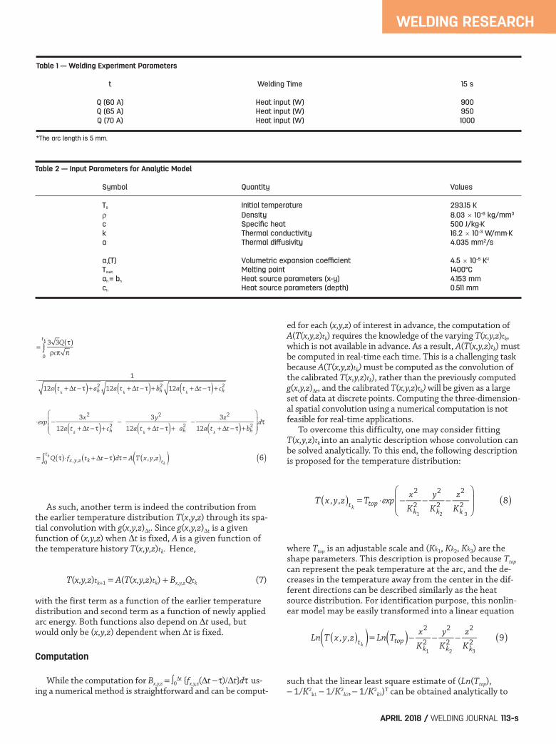
Table 1 — Welding Experiment Parameters

t Welding Time 15 s

Q (60 A) Heat input (W) 900 Q (65 A) Heat input (W) 950 Q (70 A) Heat input (W) 1000

*The arc length is 5 mm.

Table 2 — Input Parameters for Analytic Model

Symbol Quantity Values

T0 Initial temperature 293.15 K Density 8.03 × 10-6 kg/mm3

c Specific heat 500 J/kg·K k Thermal conductivity 16.2 × 10-3 W/mm·K a Thermal diffusivity 4.035 mm2/s

av(T) Volumetric expansion coefficient 4.5 × 10-5 K-1

Tmeit Melting point 1400°C ah = bh Heat source parameters (x-y) 4.153 mm ch Heat source parameters (depth) 0.511 mm


WELDING RESEARCH


calculate (Ttop, K2k1, K2

k2 , K2k3)T. (For stationary welding where

K2k1 K2

k2, the parameters can also be identified.) As such,Ttop exp( x2/K2

k1 y2/K2k2 z2/Kk3)2 becomes the analytic de-

scription of the earlier temperature distribution. Its convo-lution with g(x,y,z)t is

Subsequently, by evaluating and simplifying,

Hence, the transient temperature distribution can by re-cursively calucated when the welding current is varied.

Summary of the Recursive Analytic Model Calibratedby Measurements

In summary, the resultant analytic model that recursively

computes the temperature distribution is given by Equation4. The two terms in Equation 4 are given by Equations 5 and11, respectively. Further, Equation 11 requires parametersin the analytic description of the temperature distributionof Equation 8. These parameters are obtained by fitting theanalytic description of Equation 8 to the set of points thatrepresent the earlier temperature distribution. The resultantanalytic model is then calibrated by the measured 3D weldpool surface. The calibrated temperature distribution thenprovides the set of points to represent the “earlier tempera-ture distribution” for the next time.

Experimental Procedure

The measurement of the weld pool surface to be used forcalibration is obtained from an in-situ 3D weld pool surfacesensor developed at the University of Kentucky (Refs. 36, 37)as shown in Fig. 2. In this system, a 20-mW power illumina-tion laser with a 660-nm wavelength is used to project a 19 19 dot matrix structured light pattern on the weld pool sur-face. The mirror-like weld pool surface reflects the incidentdots following the law of reflection. The reflected dots are cap-tured by the imaging plane placed approximately 2 in. awayfrom the torch. The arc light is also reflected and captured bythe imaging plane, however, because its optic attenuation per-formance is obvious when the distance is increased, the re-flected dots can be obtained by image processing from the pic-tures captured by a CCD camera. By using a specific image pro-

A T x ,y,z( )tk( )=Ttop � Kk1

2

4a�t+Kk1

2

Kk2

2

4a�t+Kk2

2

Kk32

4a�t+Kk32

exp � x2

4a�t+Kk1

2 � y2

4a�t+Kk2

2 � z2

4a�t+Kk32

�

��

�

�� 11( )

A T x ,y,z( )tk( )= 1

(4�a�t)3/2 Ttot��+��

+��

+��

�exp � u2

Kk1

2 � v2

Kk2

2 � w2

Kk32

�

��

�

��

�exp xu( )2 + y� v( )2 + z�w( )2( )

4a�t

�

�

��

�

�

��dudvdw 10( )

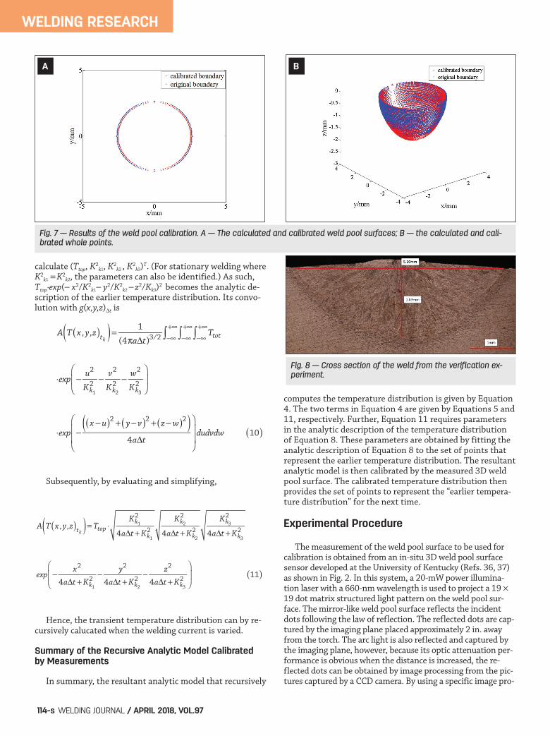
A B

Fig. 7 — Results of the weld pool calibration. A — The calculated and calibrated weld pool surfaces; B — the calculated and cali-brated whole points.

Fig. 8 — Cross section of the weld from the verification ex-periment.

.


WELDING RESEARCH


cessing and reconstruction algorithm (Ref. 38), a 3D weld poolsurface can be obtained in real time. Because the 3D weld pool surface shape (radius and convex-ity) is reconstructed in real-time, the elevation volume neededfor calibration is calculated by the following equation,

Vm Axoy H (12)

where Vm is the elevated volume from the measured weldpool surface, Axoy is the area of the weld pool surface in faceXOY, and H is the average elevation of the weld pool surface.

The average elevation above the workpiece surface is com-puted by averaging all the points inside the weld poolboundary including interpolated and original points, whichare more than 200 points in that area. With the available measurement of the 3D weld pool sur-face, the temperature distribution computed from the recur-sive solution can be calibrated similarly to the previous analyt-ic model under constant current (Ref. 1). That is, firstshrink/expand the recursively computed temperature distribu-tion T(x, y, z) in x-y directions such that T(xy*x, xy* y, z)matches the weld pool radius with that from the measured

A B

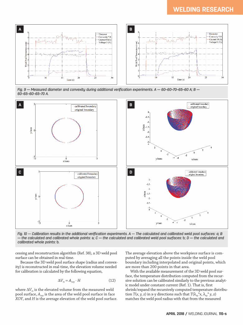
Fig. 9 — Measured diameter and convexity during additional verification experiments. A — 60–60–70–65–60 A; B —60–65–60–65–70 A.

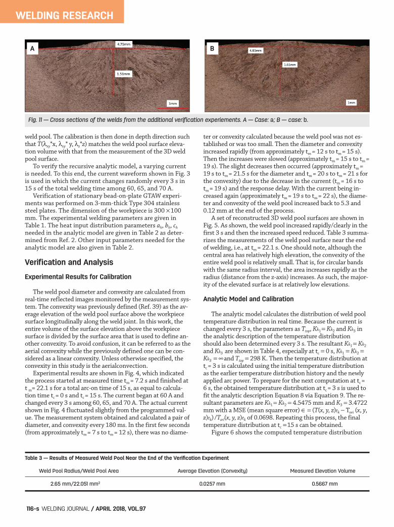
Fig. 10 — Calibration results in the additional verification experiments. A — The calculated and calibrated weld pool surfaces: a; B— the calculated and calibrated whole points: a; C — the calculated and calibrated weld pool surfaces: b; D — the calculated andcalibrated whole points: b.

A B

C D


WELDING RESEARCH


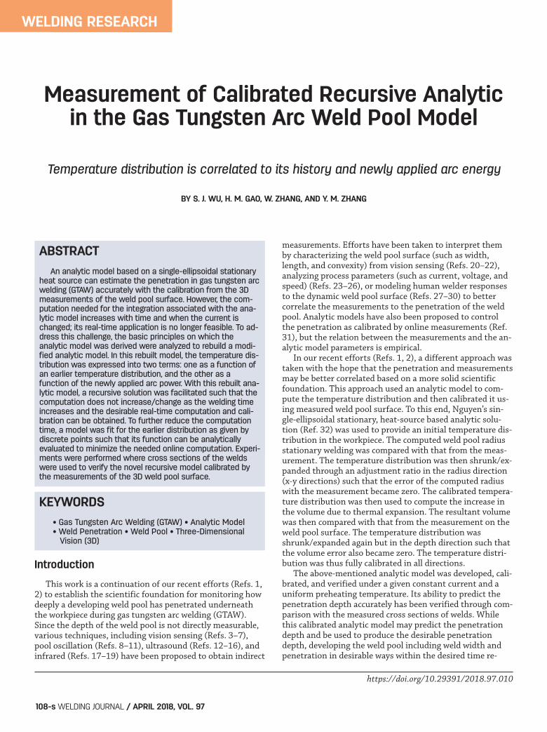
weld pool. The calibration is then done in depth direction suchthat T(xy*x, xy* y, z*z) matches the weld pool surface eleva-tion volume with that from the measurement of the 3D weldpool surface. To verify the recursive analytic model, a varying currentis needed. To this end, the current waveform shown in Fig. 3is used in which the current changes randomly every 3 s in15 s of the total welding time among 60, 65, and 70 A. Verification of stationary bead-on-plate GTAW experi-ments was performed on 3-mm-thick Type 304 stainlesssteel plates. The dimension of the workpiece is 300 100mm. The experimental welding parameters are given inTable 1. The heat input distribution parameters ah, bh, ch

needed in the analytic model are given in Table 2 as deter-mined from Ref. 2. Other input parameters needed for theanalytic model are also given in Table 2.

Verification and Analysis

Experimental Results for Calibration

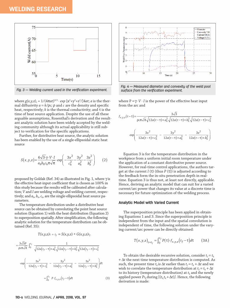
The weld pool diameter and convexity are calculated fromreal-time reflected images monitored by the measurement sys-tem. The convexity was previously defined (Ref. 39) as the av-erage elevation of the weld pool surface above the workpiecesurface longitudinally along the weld joint. In this work, theentire volume of the surface elevation above the workpiecesurface is divided by the surface area that is used to define an-other convexity. To avoid confusion, it can be referred to as theaerial convexity while the previously defined one can be con-sidered as a linear convexity. Unless otherwise specified, theconvexity in this study is the aerialconvection. Experimental results are shown in Fig. 4, which indicatedthe process started at measured time tm = 7.2 s and finished att m= 22.1 s for a total arc-on time of 15 s, as equal to calcula-tion time tc = 0 s and tc = 15 s. The current began at 60 A andchanged every 3 s among 60, 65, and 70 A. The actual currentshown in Fig. 4 fluctuated slightly from the programmed val-ue. The measurement system obtained and calculated a pair ofdiameter, and convexity every 180 ms. In the first few seconds(from approximately tm = 7 s to tm = 12 s), there was no diame-

ter or convexity calculated because the weld pool was not es-tablished or was too small. Then the diameter and convexityincreased rapidly (from approximately tm = 12 s to tm = 15 s).Then the increases were slowed (approximately tm = 15 s to tm =19 s). The slight decreases then occurred (approximately tm =19 s to tm = 21.5 s for the diameter and tm = 20 s to tm = 21 s forthe convexity) due to the decrease in the current (tm = 16 s totm = 19 s) and the response delay. With the current being in-creased again (approximately tm = 19 s to tm = 22 s), the diame-ter and convexity of the weld pool increased back to 5.3 and0.12 mm at the end of the process. A set of reconstructed 3D weld pool surfaces are shown inFig. 5. As shown, the weld pool increased rapidly/clearly in thefirst 3 s and then the increased speed reduced. Table 3 summa-rizes the measurements of the weld pool surface near the endof welding, i.e., at tm = 22.1 s. One should note, although thecentral area has relatively high elevation, the convexity of theentire weld pool is relatively small. That is, for circular bandswith the same radius interval, the area increases rapidly as theradius (distance from the z-axis) increases. As such, the major-ity of the elevated surface is at relatively low elevations.

Analytic Model and Calibration

The analytic model calculates the distribution of weld pooltemperature distribution in real time. Because the current ischanged every 3 s, the parameters as Ttop, Kk1 Kk2 and Kk3 inthe analytic description of the temperature distributionshould also been determined every 3 s. The resultant Kk1 Kk2

and Kk3 are shown in Table 4, especially at tc 0 s, Kk1 Kk2 Kk3 and Ttop 298 K. Then the temperature distribution attc = 3 s is calculated using the initial temperature distributionas the earlier temperature distribution history and the newlyapplied arc power. To prepare for the next computation at tc =6 s, the obtained temperature distribution at tc = 3 s is used tofit the analytic description Equation 8 via Equation 9. The re-sultant parameters are Kk1 Kk2 4.5475 mm and K3 3.4722mm with a MSE (mean square error) (T(x, y, z)tk Tori (x, y,z)tk)/Tori(x, y, z)tk of 0.0698. Repeating this process, the finaltemperature distribution at tc 15 s can be obtained. Figure 6 shows the computed temperature distribution

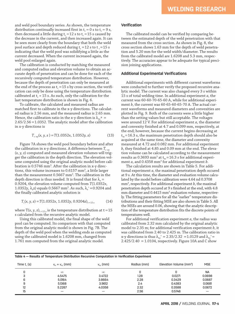
Fig. 11 — Cross sections of the welds from the additional verification experiements. A — Case: a; B — case: b.

Table 3 — Results of Measured Weld Pool Near the End of the Verification Experiment

Weld Pool Radius/Weld Pool Area Average Elevation (Convexity) Measured Elevation Volume

2.65 mm/22.051 mm2 0.0257 mm 0.5667 mm

A B


and weld pool boundary series. As shown, the temperaturedistribution continually increased first in tc = 0 s to tc = 9 s,then decreased a little during tc = 12 s to tc = 15 s caused bythe decrease in the current, and then increased again. It canbe seen more clearly from the boundary that both the weldpool surface and depth reduced during tc = 12 s to t c = 15 sindicating that the weld pool was solidifying a little as thecurrent decreased. When the current increased again, theweld pool enlarged again. The calibration is conducted by matching the measuredand computed radius and elevation volume to obtain an ac-curate depth of penetration and can be done for each of therecursively computed temperature distribution. However,because the depth of penetration can only be measured atthe end of the process as tc = 15 s by cross section, the verifi-cation can only be done using the temperature distributioncalibrated at tc = 15 s. As such, only the calibration for thelast temperature distribution is shown in Fig. 6. To calibrate, the calculated and measured radius arematched first to calibrate in the x-y directions. The calculat-ed radius is 2.56 mm, and the measured radius is 2.65 mm.Hence, the calibration ratio in the x-y direction is xy =2.65/2.56 = 1.0352. The analytic model after the calibrationin x-y directions is

Tc–xy(x, y, z ) = T(1.0352x, 1.0352y, z) (13)

Figure 7A shows the weld pool boundary before and afterthe calibration in x-y directions. A difference between Tc–xy

(x, y, z) computed and measured elevation volumes will trig-ger the calibration in the depth direction. The elevation vol-ume computed using the original analytic model before cali-bration is 0.5746 mm3. After the calibration in x-y direc-tions, this volume increases to 0.6157 mm3, a little largerthan the measurement 0.5667 mm3. The calibration in thedepth direction is thus needed. It is found that for z =0.9204, the elevation volume computed from T(1.0352x,1.0352y, zz) equals 0.5667 mm3. As such, z

= 0.9204 andthe finally calibrated analytic solution is

Tc(x, y, z) = T(1.0352x, 1.0352y, 0.9204z)t = 15 s (14)

where T(x, y, z)t = 15 s is the temperature distribution at t = 15s calculated from the recursive analytic model. Using this calibrated model, the final shape of the weldpool can be computed. Its comparison with that computedfrom the original analytic model is shown in Fig. 7B. Thedepth of the weld pool when the welding ends as computedusing the calibrated model is 1.6208 mm, changed from1.761 mm computed from the original analytic model.

Verification

The calibrated model can be verified by comparing be-tween the estimated depth of the weld penetration with thatmeasured from the cross section. As shown in Fig. 8, thecross section shows 1.63 mm for the depth of weld penetra-tion and 5.20 mm for the weld width/diameter. The resultsfrom the calibrated model are 1.6208 and 5.3 mm, respec-tively. The accuracies appear to be adequate for typical preci-sion joining applications.

Additional Experimental Verifications

Additional experiments with different current waveformswere conducted to further verify the proposed recursive ana-lytic model. The current was also changed every 3 s within15 s of total welding time. In additional experiment a, thecurrent was 60-60-70-65-60 A, while for additional experi-ment b, the current was 60-65-60-65-70 A. The actual cur-rent waveforms and measured diameters and convexities areplotted in Fig. 9. Both of the currents were a little higherthan the setting values but still acceptable. The voltageswere around 12 V. For additional experiment a, the diameterand convexity finished at 4.7 and 0.099 mm, respectively, atthe end; however, because the current begins decreasing attm = 16.3 s, the maximum penetration depth should also beacquired at the same time, the diameter and convexitymeasured at 4.72 and 0.082 mm. For additional experimentb, they finished at 4.85 and 0.09 mm at the end. The eleva-tion volume can be calculated according to the measurementresults as 0.3693 mm3 at tm = 16.3 s for additional experi-ment a, and 0.4358 mm3 for additional experiment b. The calculation results are shown in Table 5. For addi-tional experiment a, the maximal penetration depth occuredat 9 s. At this time, the diameter and evaluation volume calcu-lated by the model before calibration were 4.64 nd 0.3708mm3, respectively. For additional experiment b, the maximalpenetration depth occured at 9 s finished at the end, with 4.8mm diameter and 0.4415 mm3 evaluation volume, respective-ly. The fitting parameters for all the “earlier” temperature dis-tributions and their fitting MSE are also shown in Table 5. Allthe MSEs are around 0.06, showing that the analytic descrip-tion of the temperature distribution fits the discrete points oftemperatures well. For additional verification experiment a, the radius wascalibrated from 2.32 mm calculated by the original analyticmodel to 2.35 m; for additional verification experiment b, itwas calibrated from 2.40 to 2.425 m. The calibration ratio inx-y directions is thus xy

= 2.35/2.32 = 1.0129 and xy =

2.425/2.40 = 1.0104, respectively. Figure 10A and C show

WELDING RESEARCH


Table 4 — Results of Temperature Distribution Recursive Computation in Verification Experiment

Time tc (s) k1 = k2 (mm) k3 (mm) Radius (mm) Elevation Volume (mm3) MSE

0 ∞ ∞ 0 0 NA 3 4.5475 3.4722 1.28 0.0271 0.0698 6 5.0164 3.8664 2.28 0.3429 0.0687 9 5.1368 3.9612 2.4 0.4383 0.0681 12 5.2267 4.0358 2.32 0.3588 0.0672 15 — — 2.56 0.5746 —


the weld pool boundaries before and after the calibration inx-y directions. After the calibration in x-y directions, the ele-vation volume was increased from 0.3708 to 0.3804 mm3

and from 0.4415 to 0.4508 mm3, respectively, for a and b. Inthe subsequent calibration in the depth direction, the result-ant was z

0.9708 and 0.9667, respectively. The final cali-bration results are shown in Table 4. Using the calibration results, the weld pools were com-puted again. Figure 10B and D show the comparison of theweld pools before and after calibration. The penetration af-ter the calibration became 1.5154 and 1.5864 mm for casesa and b, respectively. The accuracy of the calibrated model can be verified bycomparing it with the measurement from the cross section. Asshown in Fig. 11A, the penetration measured from the crosssection of the weld for additional verification experiment awas 1.51 mm. It is very close to that calculated from the cali-brated model, i.e., 1.5154 mm. The error (1.51–1.5154)/1.51 0.36. From Fig. 11B, the measuredpenetration for additional verification experiment b is 1.61mm. The penetration computed from the calibrated model,1.5864 mm, is also very close to the measured penetration.The error (1.611.5864)/ 1.61 1.47. As such, the pro-posed calibration method is further considered experimentallyverified for its ability to accurately predict the depth of theweld penetration for other welding currents used.

Conclusions

The objective of this work was to continuously establish thescientific foundation to monitor how deeply a developing weldpool has penetrated underneath the workpiece during GTAW

as a follow-up to the authors’ recent efforts on the analyticmodel calibrated by the 3D measurements. To address thechallenge that the computation for the integration associatedwith the analytic model increases with time, a recursive solu-tion was derived such that the temperature distribution can becomputed from an earlier history and newly applied arc ener-gy. As a result, the computation needed to calculate the tem-perature distribution does not increase/change as the weldingtime increases. To further reduce the computation time, an an-alytic description is fit for the earlier distribution as given bydiscrete points such that the contribution of the temperaturedistribution to the present temperature distribution can beanalytically evaluated to minimize the needed online computa-tion. Verification experiments confirmed the calibrated recur-sive analytic model predicted the measured depths of weldsfrom cross sections accurately.

This work was funded in part by the National ScienceFoundation under grant NSF 1208420 and the China Schol-arship Council.

1. Wu, S., Gao, H., Zhang, W., and Zhang, Y. M. 2017. Analyticweld pool model calibrated by measurements – Part I. Welding Jour-nal 96(6): 193-s to 202-s. 2. Wu, S., Gao, H., Zhang, W., and Zhang, Y. M. Analytic weldpool model calibrated by measurements – Part II. (Accepted forpublication.)

WELDING RESEARCH


Table 5 — Temperature Distribution Parameters and Calculation Results for Additional Verification

Experiments(a) 60–60–70–65–60 A


0 ∞ ∞ 0 0 — 3 4.5475 3.4722 1.28 0.0271 0.0698 6 4.9699 3.8263 1.84 0.1201 0.0692 9 5.0626 3.8986 2.32 0.3708 0.069 12 5.1673 3.9863 2.24 0.3127 0.0678 15 — — 2.08 0.2166 —

(b) 60–65–60–65–70 A


0 ∞ ∞ 0 0 — 3 4.5475 3.4722 1.28 0.0271 0.0698 6 5.0371 3.8843 2.12 0.2380 0.0684 9 5.2114 4.0252 2.12 0.2268 0.0671 12 5.2322 4.0388 2.32 0.3589 0.0673 15 — — 2.40 0.4415 —

Table 6 — Calibration Results in Additional Verification Experiments

Current (A) xxyy zz Model

65 1.0129 0.9708 T (1.0129x, 1.0129y, 0.9708z) 60 1.0104 0.9667 T (1.0104x, 1.0104y, 0.9667z)

Acknowledgments

References


3. Mnich, C. 2004. Development of a synchronized high-speed,stereovision system for in situ weld pool measurement. MS thesis,Engineering Division, Colorado School of Mines. 4. Zhao, D. B., Yi, J. Q., et al. 2003. Extraction of three-dimension-al parameters for weld pool surface in pulsed GTAW with wire filler.Journal of Manufacturing Science and Engineering 125: 493–503.DOI:10.1115/1.1556400 5. Kovacevic, R., and Zhang, Y. M. 1996. Sensing free surface ofarc weld pool using specular reflection: Principle and analysis. Pro-ceedings of the Institution of Mechanical Engineers, Part B. Journal ofEngineering Manufacturing 210(6): 553–564. DOI:10.1243/PIME_PROC_1996_ 210_154_02 6. Zhang, Y. M., Song, H. S., and Saeed, G. 2006. Observation of adynamic specular weld pool surface. Measurement Science and Technol-ogy 17(6): L9–L12. DOI: 10.1088/0957-0233/17/6/L02 7. Song, H. S., and Zhang, Y. M. 2009. Error analysis of a three-di-mensional GTA weld pool surface measurement system. Welding Jour-nal 88(7): 141-s to 148-s. 8. Zacksenhouse, M., and Hardt, D. 1984. Weld pool impedanceidentification for size measurement and control. ASME Journal of Dy-namic Systems, Measurement, and Control 105(3): 179–184. DOI:10.1115/1.3140652 9. Anedenroomer, A. J. R., and den Ouden, G. 1998. Weld pool os-cillation as a tool for penetration sensing during pulsed GTA welding.Welding Journal 77(5): 181–187. 10. Hartman, D. A., DeLapp, D. R., Cook, G. E., and Barnett, R. J.1999. Intelligent fusion control throughout varying thermal regions.Proceedings of the IEEE Industry Applications Conference. DOI:10.1109/IAS.1999.800018 11. Yudodibroto, B., Hermans, M., Hirata, Y., and den Ouden, G.2004. Influence of filler wire addition on weld pool oscillation duringgas tungsten arc welding. Science and Technology of Welding and Joining9(2): 163–168. DOI: 10.1179/136217104225012274 12. Hardt, D. E. 1984. Ultrasonic measurement of weld penetra-tion. Welding Journal 63(9): 273-s to 285-s. 13. Carlson, N. M., and Johnson, J. A. 1988. Ultrasonic sensing ofweld pool penetration. Welding Journal 67(11): 239-s to 246-s. 14. Mi, B., and Ume, C. 2006. Real time weld penetration depthmonitoring with laser ultrasonic sensing system. Transactions ofASME: Journal of Manufacturing Science and Engineering 128(2):280–286. DOI: 10.1115/1.2137747 15. Kita, A. 2005. Measurement of weld penetration depth usingnon-contract ultrasound method. 2005. PhD dissertation, GeorgiaInstitute of Technology. pp. 22–28. 16. Dixon, S., Edwards, C., and Palmer, S. 1999. A laser-EMAT sys-tem for ultrasonic weld inspection. Ultrasonics 37(4): 273–281. DOI:10.1016/S0041-624X(99)00002-5 17. Chen, W., and Chin, B. A. 1990. Monitoring joint penetrationusing infrared sensing techniques. Welding Journal 69(4): 181-s to185-s. 18. Nagarajan, S., Chin, B. A., and Chen, W. 1992. Control of thewelding process using infrared aensor. IEEE Transactions on Roboticsand Automation 8(1): 86–93. DOI: 10.1109/70.127242 19. Wikle, H., Kottilingam, S., Zee, R., and Chin, B. 2001. Infraredsensing techniques for penetration depth control of the submergedarc welding process. Journal of Material Processing Technology 113(13):228–233. DOI: 10.1016/S0924-0136(01)00587-8 20. Vorman, A. R., and Brandt, H. 1976. Feedback control of GTAwelding using puddle width measurement. Welding Journal 55(9):742–749. 21. Ohshima, K., Yamamoto, M., Tanii, T., et. al. 1992. Digital con-trol of torch position and weld pool in MIG welding using image pro-cessing device. IEEE Transactions on Industry Applications 28(3):607–612. DOI: 10.1109/ 28.137446 22. Pietrzak, K. A., and Packer, S. M. 1994. Vision-based weld poolwidth control. Journal of Engineering for Industry-Transactions of ASME116(1): 86–92. DOI: 10.1115/ 1.2901813

23. Song, J. B., and Hardt, D. E. 1994. Dynamic modeling andadaptive control of the gas metal arc welding process. ASME J. Dy-namic Syst., Meas., Contr. 116(3): 405–413. DOI: 10.1115/1.2899235 24. Barnett, R. J., Cook, G. E., Damrongsak, D., et al. 1998.Through-the-arc sensing and control in pulsed gas metal arc welding.ASM Proceedings of the International Conference: Trends in Welding Re-search. Pine Mountain, Ga. 1068–1072. 25. Bicknell, A., Smith, J. S., and Lucas, J. 1994. Arc voltage sen-sor for monitoring of penetration in TIG welds. IEE Proceedings: Sci-ence, Measurement and Technology 141(6): 513–520. DOI: 10.1049/ip-smt:19941144 26. Wang, J. Y., Kusumoto, K., and Nezu, K. 2003. Microweld pen-etration monitoring techniques by arc sensing. Proceedings of the 2003IEEE/ASME International Conference on Advanced Intelligent Mecha-tronics 2: 1027–1030. DOI: 10.1109/AIM.2003.1225483 27. Liu, Y. K., Shao, Z., and Zhang, Y. M. 2014. Learning humanwelder movement in pipe GTAW: A virtualized welding approach.Welding Journal 93(10): 388-s to 398-s. 28. Liu, Y. K., Zhang, Y. M., and Kvidahl, L. 2014. Skilled humanwelder intelligence modeling and control: Part I – Modeling. WeldingJournal 93(2): 46-s to 52-s. 29. Liu, Y. K., Zhang, Y. M., and Kvidahl, L. 2014. Skilled humanwelder intelligence modeling and control: Part II – Analysis and con-trol applications. Welding Journal 93(5): 162-s to 170-s. 30. Liu, Y. K., Zhang, W. J., and Zhang, Y. M. 2013. Adaptive neu-ro-fuzzy inference system (ANFIS) modeling of human welder’s re-sponse to 3D weld pool surface in GTAW. Journal of ManufacturingScience and Engineering-Transactions of the ASME 135:0210101–02101011. 31. Bates, B. E., and. Hardt, D. E. 1985. A real-time calibrated ther-mal model for closed-loop weld bead geometry control. Journal of Dy-namic Systems, Measurements, and Control 107: 25–33.DOI:10.1115/1.3140703 32. Nguyen, N. T., Mai, Y. W., Simpson, S., et al. 2004. Analyticalapproximate solution for double ellipsoidal heat source in finite thickplate. Welding Journal 83(3): 82-s to 93-s. 33. Rosenthal, D. 1941. Mathematical theory of heat distributionduring welding and cutting. Welding Journal 20(5): 220-s to 234-s. 34. Goldak, J. A., Chakravarti, A., and Bibby, M. 1984. A new finiteelement model for welding heat sources. Metallurgical Transactions BVol. 15B, p. 299. DOI: 10.1007/ BF02667333 35. Eagar, T. W., and Tsai, N. S. 1983. Temperature fields producedby traveling distributed heat sources. Welding Journal 62(12): 346-s to355-s. 36. Saeed, G., and Zhang, Y. M. 2008. Weld pool surface depthmeasurement using a calibrated camera and structured light. Meas-urement Science and Technology 18: 2570–2578. DOI:10.1088/0957-0233/18/8/033 37. Song, H. S., and Zhang, Y. M. 2007. Three-dimensional recon-struction of specular surface for gas tungsten arc weld pool. Measure-ment Science & Technology 18: 3751–3767. DOI:10.1088/0957-0233/18/12/010 38. Liu, Y. K., Zhang, W. J., and Zhang, Y. M. 2015. Nonlinearmodeling for 3D weld pool characteristic parameters in GTAW. Weld-ing Journal 94(7): 231-s to 240-s. 39. Zhang, W. J., Liu, Y. K., Wang, X. W., and Zhang, Y. M.2012.Characterization of three-dimensional weld pool surface in gas tung-sten arc welding. Welding Journal 91(7): 195-s to 203-s.

WELDING RESEARCH


SHAO JIE WU is with the Harbin Institute of Technology, Harbin,China, and the University of Kentucky, Lexington, Ky. HONGMING GAO is with the Harbin Institute of Technology, Harbin,China. WEI ZHANG is with The Ohio State University, Columbus,Ohio. YU MING ZHANG ([email protected]) is with the Uni-versity of Kentucky, Lexington, Ky.


Documents

Measurement of Calibrated Recursive Analytic in the …...• Gas Tungsten Arc Welding (GTAW) • Analytic Model • Weld Penetration • Weld Pool • Three-Dimensional Vision (3D)