Measurement of gas gain fluctuations

M. Chefdeville, LAPP, AnnecyTPC Jamboree, Orsay, 12/05/2009

Overview• Introduction– Motivations, questions and tools

• Measurements– Energy resolution & electron collection efficiency

Micromegas-like mesh readout– Single electron detection efficiency and gas gain

TimePix readout

• Conclusion

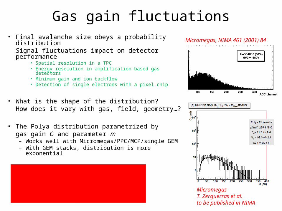
Gas gain fluctuations• Final avalanche size obeys a probability distribution

Signal fluctuations impact on detector performance

• Spatial resolution in a TPC• Energy resolution in amplification-based gas detectors• Minimum gain and ion backflow• Detection of single electrons with a pixel chip

• What is the shape of the distribution?How does it vary with gas, field, geometry…?

• The Polya distribution parametrized bygas gain G and parameter m– Works well with Micromegas/PPC/MCP/single GEM– With GEM stacks, distribution is more exponential

Micromegas, NIMA 461 (2001) 84

MicromegasT. Zerguerras et al.to be published in NIMA

= b, relative gain variance

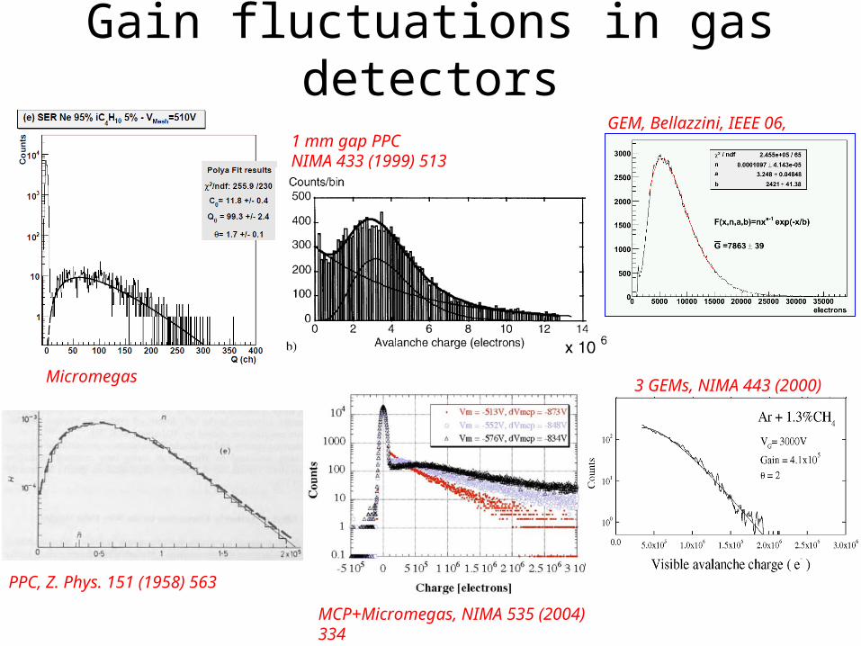
Gain fluctuations in gas detectors

Micromegas

1 mm gap PPCNIMA 433 (1999) 513

3 GEMs, NIMA 443 (2000) 164

GEM, Bellazzini, IEEE 06, SanDiego

PPC, Z. Phys. 151 (1958) 563

MCP+Micromegas, NIMA 535 (2004) 334

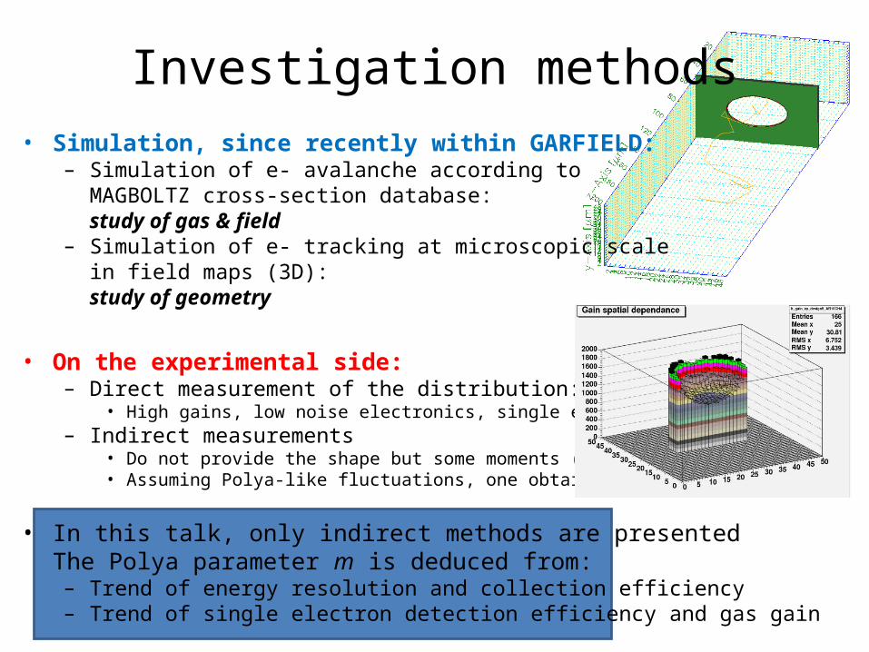
Investigation methods• Simulation, since recently within GARFIELD:

– Simulation of e- avalanche according toMAGBOLTZ cross-section database:study of gas & field

– Simulation of e- tracking at microscopic scalein field maps (3D):study of geometry

• On the experimental side:– Direct measurement of the distribution:

• High gains, low noise electronics, single electron source– Indirect measurements

• Do not provide the shape but some moments (variance)• Assuming Polya-like fluctuations, one obtains the shape

• In this talk, only indirect methods are presentedThe Polya parameter m is deduced from:– Trend of energy resolution and collection efficiency– Trend of single electron detection efficiency and gas gain

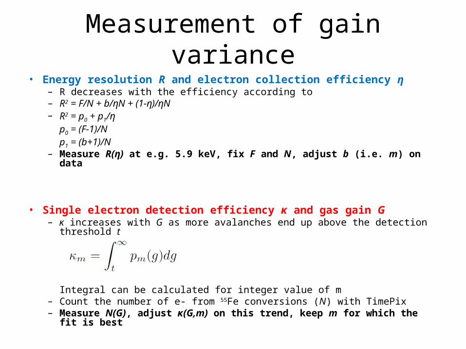
Measurement of gain variance• Energy resolution R and electron collection efficiency η

– R decreases with the efficiency according to– R2 = F/N + b/ηN + (1-η)/ηN– R2 = p0 + p1/η

p0 = (F-1)/Np1 = (b+1)/N

– Measure R(η) at e.g. 5.9 keV, fix F and N, adjust b (i.e. m) on data

• Single electron detection efficiency κ and gas gain G– κ increases with G as more avalanches end up above the detection threshold t

Integral can be calculated for integer value of m– Count the number of e- from 55Fe conversions (N) with TimePix– Measure N(G), adjust κ(G,m) on this trend, keep m for which the fit is best

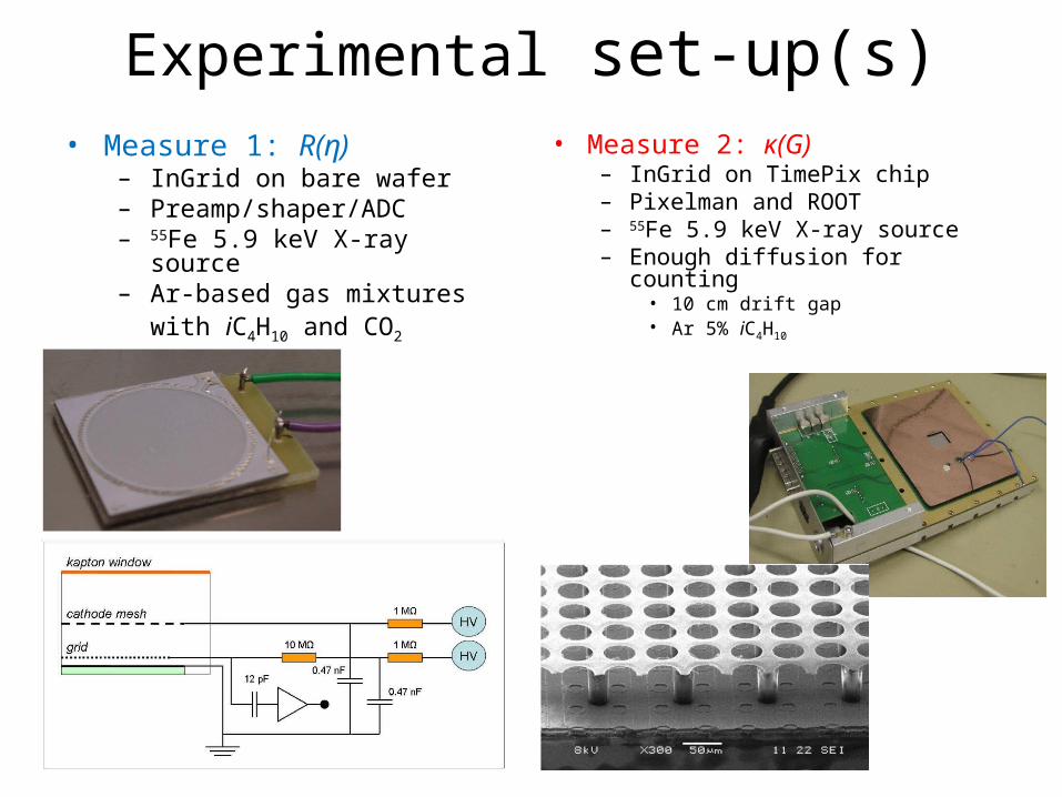
Experimental set-up(s)• Measure 1: R(η)

– InGrid on bare wafer– Preamp/shaper/ADC– 55Fe 5.9 keV X-ray source– Ar-based gas mixtures

with iC4H10 and CO2

• Measure 2: κ(G)– InGrid on TimePix chip– Pixelman and ROOT– 55Fe 5.9 keV X-ray source– Enough diffusion for counting

• 10 cm drift gap• Ar 5% iC4H10

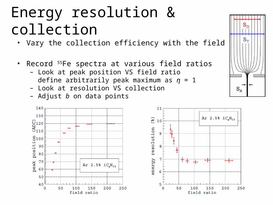
Energy resolution & collection• Vary the collection efficiency with the field ratio

• Record 55Fe spectra at various field ratios– Look at peak position VS field ratio

define arbitrarily peak maximum as η = 1– Look at resolution VS collection– Adjust b on data points

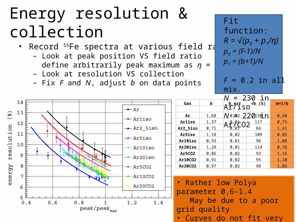
Energy resolution & collection• Record 55Fe spectra at various field ratios

– Look at peak position VS field ratiodefine arbitrarily peak maximum as η = 1

– Look at resolution VS collection– Fix F and N, adjust b on data points

Fit function:R = √(p0 + p1/η)p0 = (F-1)/Np1 = (b+1)/N

F = 0.2 in all mix.N = 230 in Ar/isoN = 220 in Ar/CO2

Gas b b_err √b (%) m=1/b

         

Ar 1,68 0,02 130 0,60

Ar1iso 1,37 0,01 117 0,73

Ar2_5iso 0,71 0,01 84 1,41

Ar5iso 1,18 0,02 109 0,85

Ar10iso 0,93 0,01 96 1,08

Ar20iso 1,29 0,01 114 0,78

Ar5CO2 0,86 0,02 93 1,16

Ar10CO2 0,91 0,02 95 1,10

Ar20CO2 0,97 0,02 98 1,03

• Rather low Polya parameter 0.6-1.4 May be due to a poor grid quality• Curves do not fit very well points Could let F or/and N free

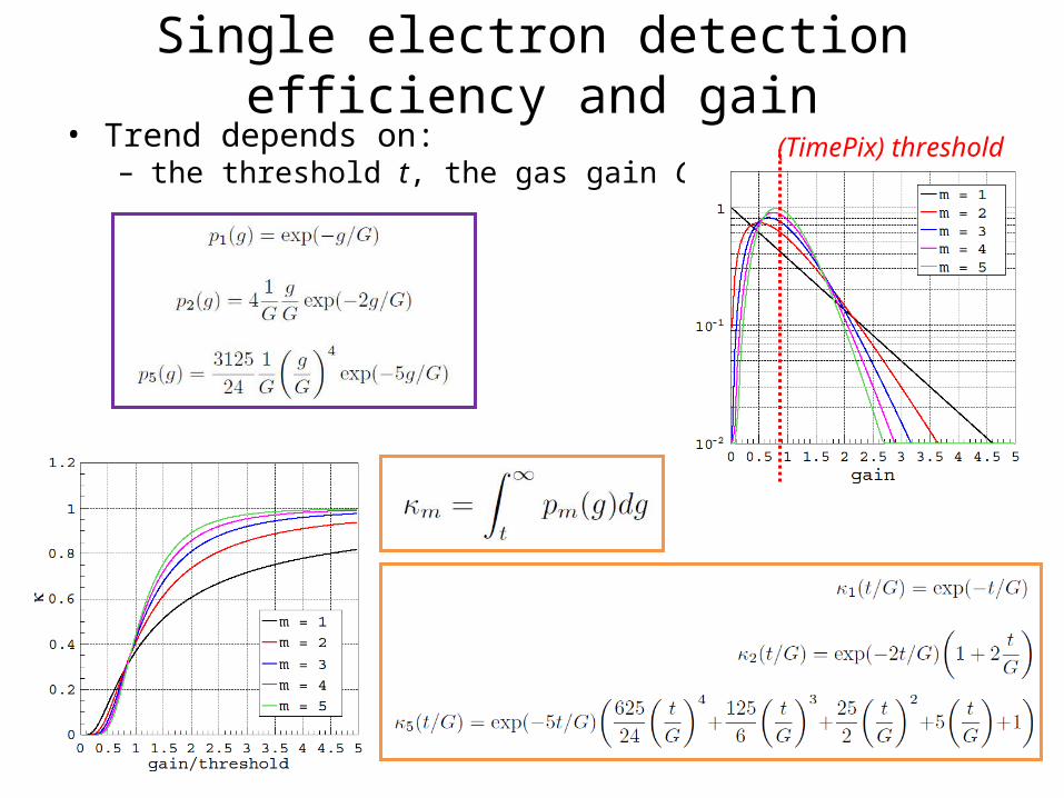
Single electron detection efficiency and gain• Trend depends on:

– the threshold t, the gas gain G and m(TimePix) threshold

Single electron detection efficiency and gain

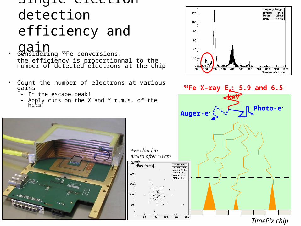
• Considering 55Fe conversions:the efficiency is proportionnal to the number of detected electrons at the chip

• Count the number of electrons at various gains– In the escape peak!– Apply cuts on the X and Y r.m.s. of the hits

55Fe X-ray E0: 5.9 and 6.5 keV

Photo-e-

TimePix chip

Auger-e-

55Fe cloud in Ar5iso after 10 cm drift

Single electron detection efficiency and gain

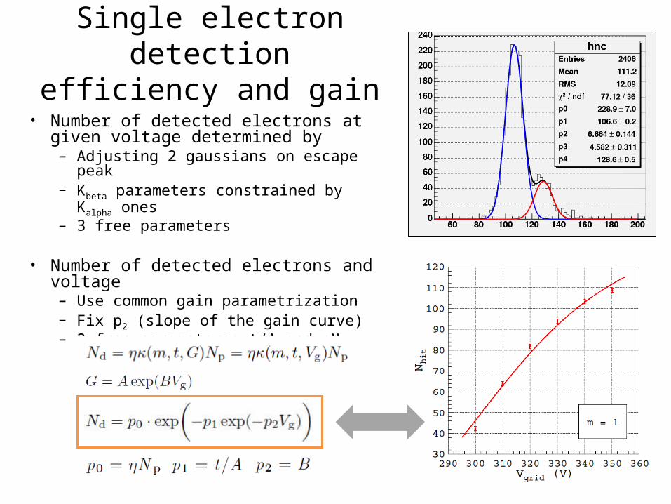
• Number of detected electrons at given voltage determined by– Adjusting 2 gaussians on escape peak– Kbeta parameters constrained by Kalpha ones– 3 free parameters

• Number of detected electrons and voltage– Use common gain parametrization– Fix p2 (slope of the gain curve)– 2 free parameters: t/A and ηN

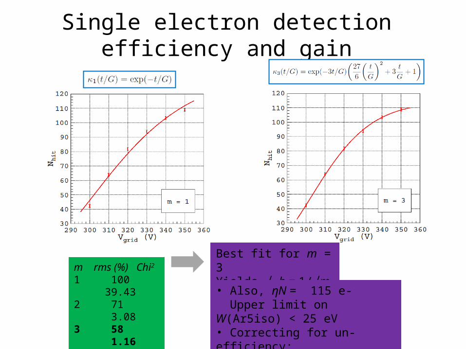
Single electron detection efficiency and gain

m rms (%) Chi2

1 100 39.432 71 3.083 58 1.164 50 1.415 45 1.60

Best fit for m = 3Yields √ b = 1/√m ~ 58 %

• Also, ηN = 115 e- Upper limit on W(Ar5iso) < 25 eV• Correcting for un-efficiency: Upper limit on F(Ar5iso) < 0.3

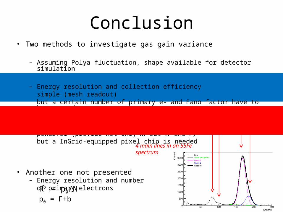
Conclusion• Two methods to investigate gas gain variance

– Assuming Polya fluctuation, shape available for detector simulation

– Energy resolution and collection efficiencysimple (mesh readout)but a certain number of primary e- and Fano factor have to be assumed

– Single e- detection efficiency and gainpowerful (provide not only m but W and F)but a InGrid-equipped pixel chip is needed

• Another one not presented– Energy resolution and number

of primary electronsR2 = p0/Np0 = F+b

4 main lines in an 55Fe spectrum