Measurement of Strain in the Left Ventricle during ... · PDF fileMeasurement of Strain in the Left Ventricle during Diastole with cine ... linear and undergoes finite deformation

BIO-04-1249 Veress, et al. 1

Measurement of Strain in the Left Ventricle during Diastole with cine-MRI and Deformable Image Registration

*Alexander I. Veress, +Grant T. Gullberg, *Jeffrey A. Weiss

*Department of Bioengineering, and Scientific Computing and Imaging Institute

University of Utah Salt Lake City, UT

+E. O. Lawrence Berkeley National Laboratory

Berkeley, CA

Final Version for Publication, Journal of Biomechanical Engineering July 26, 2005

Keywords: strain, left ventricle, deformable image registration, soft tissue mechanics, finite element, magnetic resonance imaging Corresponding Author: Jeffrey A. Weiss, Ph.D. Department of Bioengineering University of Utah 50 South Central Campus Drive, Room 2480 Salt Lake City, Utah 84112-9202 801-587-7833 [email protected]


ABSTRACT

The assessment of regional heart wall motion (local strain) can localize ischemic

myocardial disease, evaluate myocardial viability and identify impaired cardiac function due to

hypertrophic or dilated cardiomyopathies. The objectives of this research were to develop and

validate a technique known as Hyperelastic Warping for the measurement of local strains in the 5

left ventricle from clinical cine-MRI image datasets. The technique uses differences in image

intensities between template (reference) and target (loaded) image datasets to generate a body

force that deforms a finite element (FE) representation of the template so that it registers with the

target image. To validate the technique, MRI image datasets representing two deformation states

of a left ventricle were created such that the deformation map between the states represented in 10

the images was known. A beginning diastolic cine-MRI image dataset from a normal human

subject was defined as the template. A second image dataset (target) was created by mapping the

template image using the deformation results obtained from a forward FE model of diastolic

filling. Fiber stretch and strain predictions from Hyperelastic Warping showed good agreement

with those of the forward solution (R2 = 0.67 stretch, R2 = 0.76 circumferential strain, R2 = 0.75 15

radial strain and R2 = 0.70 in-plane shear). The technique had low sensitivity to changes in

material parameters (∆R2 = -0.023 fiber stretch, ∆R2 = -0.020 circumferential strain, ∆R2 = -0.005

radial strain, and ∆R2 = 0.0125 shear strain with little or no change in RMS error), with the

exception of changes in bulk modulus of the material. The use of an isotropic hyperelastic

constitutive model in the Warping analyses degraded the predictions of fiber stretch. Results 20

were unaffected by simulated noise down to an SNR of 4.0 (∆R2 = -0.032 fiber stretch, ∆R2 = -

0.023 circumferential strain, ∆R2 = -0.04 radial strain, and ∆R2 = 0.0211 shear strain with little or


no increase in RMS error). This study demonstrates that Warping in conjunction with cine-MRI

imaging can be used to determine local ventricular strains during diastole.

INTRODUCTION

Left ventricular (LV) wall function is typically evaluated by the measurement of global 5

measures of ventricular deformation such as ejection fraction, and by local estimates of wall

deformation such as wall motion and wall thickening. Techniques that have been employed

include 2-D Doppler echocardiography [1,2], cine-MRI [3] and radionuclide ventriculography

[4]. Global measures of ventricular function such as ejection fraction do not provide information

on the location of functional deficits. Wall motion and wall thickening analyses provide useful 10

local measures of wall function but are at best an indirect measure of local tissue contraction and

dilation.

The measurement of local wall deformation (strain) or fiber contraction/extension

(stretch) can provide insight into local myocardial pathologies such as ischemia. While tagged

MRI can measure local deformation [5], fiber stretch cannot be determined without a model 15

representing the mechanics of the myocardium [6]. Similarly, displacement measurements made

by tracking the epi- and endocardial surfaces with cine-MRI have been combined with an

anisotropic linear elasticity model to estimate fiber stretch and myocardial strain [7]. However,

myocardial tissue is non-linear and undergoes finite deformation [8]. Alternatively, the strain

tensor information may be reoriented to the fiber coordinate system. Tseng coregistered 20

diffusion tensor MR (fiber distribution) and strain rate MR to obtain fiber stretch estimates for

the mid-ventricle [9]. However, the strain tensor information was based on 2-D strain rate

measurements and was applied only to the mid-ventricle rather than the entire LV.


Hyperelastic Warping, a technique for deformable image registration, allows the

determination of local tissue deformation from pairs or sequences of medical image data [10-13].

Deformable image registration techniques determine a deformation map that registers a template

and target image. In Hyperelastic Warping, a discretized template image is defined as a

hyperelastic material governed by nonlinear continuum mechanics. This ensures that mappings 5

from template to target are diffeomorphic (one-to-one, onto, differentiable and invertible) [14].

The technique has been used to determine strain from sequences of images of deforming tissue

without the need for markers [10] or other fiducials such as MR tags, and in theory it can be used

with any type of unimodal image data.

The objectives of this study were to develop and validate the use of Hyperelastic Warping 10

for the extraction of high-resolution strain maps of the left ventricle from cine-MRI images. The

sensitivity of predictions to errors in material model selection, material parameters and simulated

noise in the image data was determined. The hypotheses were that 1) Hyperelastic Warping

could accurately predict the fiber stretch (final length/initial length along the local fiber

direction) and in-plane strain distributions during diastolic (passive) filling from cine-MRI image 15

datasets, 2) variations in the assumed material properties and constitutive model would have a

minimal effect on the predicted fiber stretch distribution and 3) the results of Warping cardiac

cine-MRI images would be relatively insensitive to noise in the image data.

MATERIALS AND METHODS 20

Finite Deformation Theory. A Lagrangian reference frame is assumed. The template and

target images have spatially varying scalar intensity fields, denoted by T and S, respectively. The


deformation map is ϕ(X) = x = X + u(X), where x are current (deformed) coordinates

corresponding to X and u(X) is the displacement field. F is the deformation gradient:

( )( )∂

=∂

XF X

Xϕ

. (1)

The change in density is related to F through the Jacobian, ( ) 0: detJ ρ ρ= =F , where 0ρ and

ρ are densities in the reference and deformed configurations, respectively. The positive 5

definite, symmetric left Cauchy-Green deformation tensor is T=C F F .

Variational Framework for Deformable Image Registration. Most deformable image

registration methods can be posed as the minimization of an energy functional E with two terms:

( ) ( ) ( ) ( )( ), , , ,dv dvE W U T SJ J

= +∫ ∫β β

X X Xϕ ϕ ϕ ϕ . (2)

W provides regularization and/or some constraint on the deformation map (e.g., one-to-one 10

mapping or no negative volumes), while U depends on the registration of the template (T) and

target (S) image data. β is the volume of integration in the deformed configuration.

The Euler-Lagrange equations are obtained by taking the first variation of E(ϕ) with

respect to the deformation ϕ in the direction η , denoted εη , where ε is an infinitesimal scalar,

and then letting 0ε → [15]. The first variation of the first term in (2) defines the forces per unit 15

volume from the regularization, while the second term in (2) gives rise to an image-based force

term:

( ) : 0W dv U dvGJ Jβ β

∂ ∂= ⋅ + ⋅ =

∂ ∂∫ ∫ϕ,η η ηϕ ϕ

. (3)

Equation (3) is a highly nonlinear function of the deformation ϕ . An incremental-

iterative solution method is necessary to obtain the deformation map ϕ that satisfies the 20


equation. The most common approach is based on Newton’s method. Assuming that a solution

*ϕ is known, a solution is sought at * + ∆uϕ where ∆u is a variation in the configuration (virtual

displacement). The linearization of (3) at *ϕ in the direction ∆u is defined as:

( ) ( ) ( )* : W U dv dvL G G DGJ Jβ β

∂ ∂⎛ ⎞= + ⋅ ∆ = ⋅ + + ⋅ + ⋅⎜ ⎟∂ ∂⎝ ⎠

∫ ∫u u∆∗ ∗ϕ

ϕ ,η ϕ ,η η ηϕ ϕ

D k , (4)

where 2

: U∂=

∂ ∂ϕ ϕk is the image stiffness and

2

: W∂=

∂ ∂ϕ ϕD is the regularization stiffness. 5

Particular Forms for W and U – Hyperelastic Warping. In hyperelastic Warping, a

spatial discretization of the template image is deformed into alignment with the target image.

The target image remains fixed with respect to reference configuration and does not change over

the course of the analysis. Assuming that T is not changed by the deformation it is represented

as T(X). The values of S at the material points associated with the deforming template change as 10

the template deforms with respect to the target; it is written as S(ϕ). In other words, from the

perspective of the material points associated with the template image, the target intensity changes

with deformation while the template intensity does not. The standard formulation uses a

Gaussian sensor model for the image energy [14]:

( ) ( ) ( )( )2,

2U T Sλ

= −X Xϕ ϕ . (5) 15

λ is a penalty parameter that enforces alignment of the template model with the target image. As

λ → ∞ , ( ) ( )( )20T S− →X ϕ , and the image energy converges to a finite, minimized value.

Hyperelastic Warping assumes that W is the hyperelastic strain energy from continuum

mechanics. Since W depends on C, which is independent of rotation, hyperelasticity provides an


objective (invariant under rotation) constitutive framework. With these specific assumptions,

equation (2) takes the form:

( ) ( ) ( ) ( )( ), ,dv dvE W U T SJ J

= −∫ ∫β β

X C Xϕ ϕ . (6)

The first variation of the first term in (6) yields the weak form of the momentum equations for

nonlinear solid mechanics (see, e.g., [15]). The first variation of the functional U in (5) gives 5

rise to the image-based force term:

( ) ( ) ( )( ) ( ),S

DU T Sλ∂⎡ ⎤

⋅ = − − ⋅⎢ ⎥∂⎣ ⎦X X

ϕϕ η ϕ η

ϕ. (7)

This term drives the template deformation based on pointwise differences in image intensity and

the gradient of the target intensity, evaluated at material points in the template model. A similar

computation for the term W leads to the weak form of the momentum equation (see, e.g., [16]): 10

( ) ( ) ( ): : 0S dvG DE dv T SJβ β

λ ⎡ ⎤∂= ⋅ = ∇ − − ⋅ =⎢ ⎥∂⎣ ⎦

∫ ∫ϕ,η ϕ η σ η ηϕ

. (8)

Here, “:” denotes the tensor inner product and σ is the 2nd order symmetric Cauchy stress tensor,

1 TWJ

∂=

∂F F

Cσ . (9)

Thus, the image-based forces are opposed by internal forces, arising from the constitutive model.

The linearization of equation (8) at *ϕ in the direction ∆u yields: 15

( ) ( )

( ) ( )

* :

: : ∆ : : ∆ ∆s s

S dvL G dv T SJ

dvdv dvJ

β β

β β β

λ ⎡ ⎤∂= ∇ − − ⋅⎢ ⎥∂⎣ ⎦

+ + + ⋅ ⋅

∫ ∫

∫ ∫ ∫u u u

∗ϕϕ,η σ η η

ϕ

η σ η η∇ ∇ ∇ ∇c k . (10)

Here, c is the 4th order spatial elasticity tensor [15] and [ ]s ⋅∇ is the symmetric gradient operator:


[ ] [ ] [ ]12

Ts

⎡ ⎤∂ ⋅ ∂ ⋅⎛ ⎞⋅ = +⎢ ⎥⎜ ⎟∂ ∂⎢ ⎥⎝ ⎠⎣ ⎦ϕ ϕ

∇ . (11)

The first two terms in the second line of equation (10) are geometric and material stiffnesses,

respectively, from computational mechanics [17]. The image stiffness (2nd order tensor) is:

( )2 2

: U S S ST S∂ ∂ ∂ ∂λ∂ ∂ ∂ ∂

⎡ ⎤⎛ ⎞⎛ ⎞ ⎛ ⎞= = ⊗ − −⎢ ⎥⎜ ⎟⎜ ⎟ ⎜ ⎟∂ ∂ ⎝ ⎠ ⎝ ⎠ ⎝ ⎠⎣ ⎦ϕ ϕ ϕ ϕ ϕ ϕ

k , (12)

where “⊗” represents the vector outer product operation. 5

FE Discretization: A FE mesh is constructed to correspond to all or part of the template

image. T is interpolated to the nodes of the FE mesh. As the mesh deforms, S is queried at the

current location of nodes in the template FE mesh. An isoparametric conforming FE

approximation is introduced for η and u∆ in equation (10):

( ) ( )nodes nodes

1 1

: | , : |e e

N N

e j j e j jj j

N NΩ Ω= =

= = ∆ = ∆ = ∆∑ ∑ξ u u ξ uη η η , (13) 10

where the subscript e specifies that variations are restricted to an element with domain Ωe, and

Nnodes is the number of element nodes. Eight-node hexahedral elements with three translational

degrees of freedom per node were used, so ( ) ( ) ( ) 1,1 1,1 1,1∈ − × − × −ξ is the bi-unit cube, and

Nj are the isoparametric shape functions. The gradients of η are discretized as

nodes nodes

1 1

,N N

L NLs j j j j

j j= =

= =∑ ∑η B η η B η∇ ∇ , (14) 15

where BL and BNL are the linear and nonlinear strain-displacement matrices in Voigt notation

[18]. For an assembled FE mesh, equation (10) becomes (in Voigt notation):

( ) ( )( ) ( ) ( )( )nodes nodes nodes

* * ext * int *

1 1 1

N N NR I

ji j i iij= = =

+ ⋅ ∆ = −∑ ∑ ∑K K u F Fϕ ϕ ϕ ϕ . (15)


Equation (15) is a system of linear equations. The term in parentheses on the left-hand side is

the (symmetric) tangent stiffness matrix. ∆u is the vector of unknown incremental nodal

displacements with length [ ]8 3 elN× × , where elN is the number of elements. extF is the

external force vector arising from equation (7), and intF is the internal force vector from the

stress divergence. The regularization stiffness arising from the hyperelastic energy is: 5

( ) ( )T TR NL NL L Ldv dv= +∫ ∫β β

K B σB B Bc . (16)

The image-based stiffness is:

JI T dv

β

= ∫K N Nk . (17)

An initial estimate of ∆u is obtained by inverting equation (15), and this solution is improved

iteratively using a quasi-Newton method [19]. 10

Solution Procedure and Augmented Lagrangian: In equation (6), the image data may be

treated as either a soft constraint, with the mechanics providing the “truth”, or as a hard

constraint, with the mechanics providing regularization, or as a combination. Indeed, equation

(5) is essentially a penalty function stating that the template and target image intensity fields

must be equal as → ∞λ . However, as λ is increased, KI becomes ill-conditioned, resulting in 15

inaccurate estimates for 1I−K , which leads to slowed convergence or divergence of the nonlinear

iterations. To circumvent this problem, the augmented Lagrangian method was used [20] . A

solution at a particular timestep is first obtained with a relatively small penalty λ. The image-

based body forces U∂ ∂ϕ are incrementally increased in a second iterative loop, resulting in

progressive satisfaction of the constraint. This algorithm allows the constraint to be satisfied to a 20


user-defined tolerance and avoids ill conditioning. Equation (8) is modified by addition of an

image-based force γ due to the augmentation:

( )* 0dvG GJβ

= + ⋅ =∫ ηϕ,η γ (18)

The augmented Lagrangian update procedure for timestep n+1 takes the form:

( )

( )

01

11 1 1

*1

11 1 1

0

DO for each augmentation WHILE TOL

Minimize with fixed using the BFGS method

Update mutipliers using

END DO

n n

k k kn n n

kn

kk kn n n

k

k

G

U

γ γ

γ γ γ

γ

γ γ ϕ

+

++ + +

+

++ + +

==

− >

= + ∂ ∂

(19) 5

Here, 01n+γ is the starting value for the multiplier vector at time n+1 before the beginning of

augmentations, k is the augmentation number and TOL is the tolerance for defining convergence

of the augmentations. This nested iteration procedure (Uzawa algorithm, [20]) converges

quickly because the multipliers γ are fixed during minimization of G*. For the present study,

augmentations were performed after λ was increased to the maximum value that could be used 10

without numerical ill conditioning. After this, the augmented Lagrangian method was used with

TOL = 0.20.

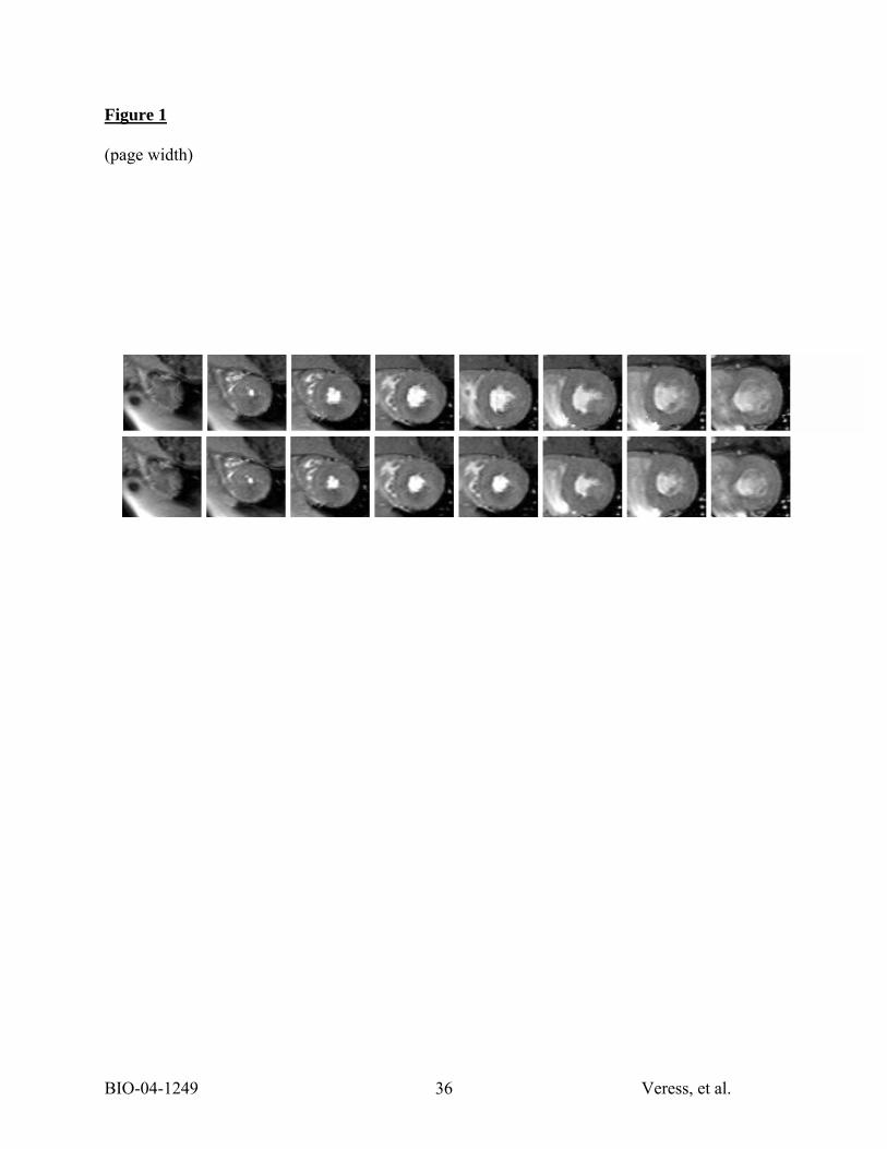
Cardiac Image Acquisition: To mimic typical clinical MR acquisition for patients with

cardiac pathologies, gated cine-MRI images of a normal male volunteer’s heart (35 years old) were

acquired on a 1.5T Siemens scanner using standard clinical settings (256×256 image matrix, 378 15

mm FOV, 10 mm slice thickness, 10 slices) (Figure 1). The MRI dataset corresponding to

beginning of diastole was designated as the template image. The template image was cropped to a

64×64 image matrix by 8 slices to focus on the heart.


FE Mesh Generation and Boundary Conditions. The boundaries of the LV were obtained

by manual segmentation of the epi- and endocardium from the template image. The 3-D FE model

was constructed to include the entire image domain, with the lumen and the tissue surrounding the

myocardium represented as an isotropic hyperelastic material with relatively soft properties

(modulus of elasticity E = 0.3 KPa and Poisson’s ratio ν = 0.3) so that the entire template image 5

could be mapped. The edges of the mesh were fixed, eliminating rigid motion.

Constitutive Model and Material Coefficients. The myocardium was represented as

transversely isotropic hyperelastic with fiber angle varying from –90o at the epicardial surface to

90o at the endocardial surface [21]. The model represented fibers in a neo-Hookean matrix:

21 2( 3) ( ) [ln( )]

2KW I F Jµ λ= − + +%% . (20) 10

1I% is the first deviatoric invariant of C [22], 0 0λ = ⋅ ⋅a C a% % is the deviatoric fiber stretch along

the local direction a0, µ is the shear modulus of the matrix and K is the bulk modulus. The fiber

stress-stretch behavior was represented as exponential, with no resistance to compressive load:

( )( )

2

23 4

0, 1,

exp 1 1 , 1.

F

F C C

λ λλ

λ λ λλ

∂= <

∂∂ ⎡ ⎤= − − ≥⎣ ⎦∂

% %%

% % %%

(21)

Here, C3 scales the stresses and C4 defines the fiber uncrimping rate. A description of the 15

constitutive model and its FE implementation can be found in Weiss et al. [23].

Material coefficients were determined by a nonlinear least squares fit of the constitutive

equation to published equibiaxial stress/strain curves [24] (µ = 2.10 KPa, C3 = 0.14 KPa, and C4

=22.0). A bulk modulus K of 160.00 KPa was chosen so that changes in relative volume were

under 5%, in other words the material would be nearly incompressible. The LV material 20

properties do not need to be exact for this analysis because stretch and strains from the forward


FE model were used as the “gold standard” for comparison to Warping results. A physiological

internal pressure was applied to the endocardial surface and a nonlinear FE analysis was

performed using NIKE3D [25]. Predictions of fiber stretch, circumferential, radial and in-plane

(radial-circumferential) shear strains were compared to values in the literature.

Creation of Synthetic Target Image: To validate Warping predictions of strain, a pair of 5

3D MRI image datasets representing two deformation states of the LV were used such that the

deformation map between the states represented in the images was known. A synthetic target

image was created by applying the displacement map of the forward FE model to the template

MRI image (Figure 1). These image datasets were used as the only input in the Warping

analysis; pressure boundary conditions were not applied. 10

Comparison of Synthetic End-diastolic Image with In Vivo End-diastolic image data set:

The simulated end-diastolic image data set (Target) and the in vivo end-diastolic image data set

were compared to determine the similarity of the images using two standard image similarity

measures that are independent of the image energy functional: the Hausdorff Distance [26] and

the Chamfer Distance [27]. These measures were also determined for the template image data 15

set and the in vivo image data set for comparison purposes. The Chamfer Distance is the average

distance (in pixels) for every edge point in one image to the nearest edge in the other. The

Hausdorff Distance [26] gives the maximum distance over all of the edge points in one image to

the nearest edge in the other image (it gives the distance for that edge which is farthest to the

nearest edge in the other image). The Hausdorff Distance gives the "worst case" of mismatch 20

between two images. It should be noted that the forward model, which the synthetic image data

set was based upon, was not designed to reproduce the deformation documented in the in vivo


image data set. Rather, it was designed to have deformation values during diastole that were

consistent with those reported in the literature.

Warping Model: The Warping FE model used the same geometry and material properties

as the forward FE model. The tether mesh was not included because it was only necessary to

determine deformation measures within the LV wall. Nodal values of fiber stretch, 5

circumferential, radial and shear strain were averaged for each image slice and compared with

values from the forward FE model. To assess transmural deformation, the same measures were

computed as a function of wall position. Scatter plots were generated to determine coefficients

of determination (R2) between Warping and forward FE model predictions. A Bland-Altman

analysis [28] was performed to assess agreement between the forward FE and Warping 10

predictions for the four measures of deformation. Absolute and percent RMS errors were

calculated using:

nodes2

forward Warp1nodes

1RMS error ( )N

iNε ε

=

= −∑ , (22)

and

nodes 2forward Warp

21 forward

( )percent RMS error

( )

N

i

ε εε=

−= ∑ . (23) 15

Here, forwardε represents a forward analysis strain value for a given node, Warpε is the predicted

strain value for the corresponding node in the Warping analysis and nodesN is the total number of

nodes in the elements representing the myocardial wall. For fiber stretch, percent RMS error

was calculated by first subtracting a value of 1.0 from the data to convert stretch to units of

strain. 20


Edge versus Wall Warping Solution: Since the Warping body force is based on image

intensity and gradient (Equation (7)), it was expected that predictions would be more accurate for

the endo- and epicardial boundaries in comparison to mid-wall. R2 values were calculated

between the strain/stretch Warping and FE predictions for nodes on the endo- and epicardial

surfaces. These R2 values were compared with values for the entire model on each image plane. 5

Sensitivity to Material Coefficients and Constitutive Model: To determine the sensitivity

of Warping to changes in material coefficients, µ and C3 were increased and decreased by 24%

of the baseline values, corresponding to the 95% confidence interval of the data in Humphrey et

al. [29]. To assess the importance of the fiber reinforcement, the constitutive model was changed

to an isotropic neo-Hookean model for the Warping simulations. Finally, the effect of the 10

material bulk modulus was assessed by increasing and decreasing K by a factor of 10.0 in the

Warping analysis. To measure the effect of the changes in material properties and the change in

material model, the R2 values, RMS errors and the percent RMS errors were determined for the

four measures of local strain between the Warping and forward FE model predictions.

Sensitivity to Image Noise: To assess the effects of noise on the Warping predictions, an 15

additive noise model was used to modify the images [30]. Random noise ( ),N i j was added to

the images ( ),I i j , where i and j represent pixel coordinates, to create a noisy image ( ),S i j :

( ) ( ) ( ), , ,S i j I i j N i j= + . (24)

( ),N i j was defined as the standard deviation Nσ of a zero mean normal probability distribution

for noise image intensities [30]. The signal to noise ratio (SNR) was defined as: 20

N

ISNRσσ

= . (25)


For the images used, Iσ = 42 gray levels. SNRs of 16, 8, 4, 1, and 0.5 were examined (Figure

3). The measures of deformation obtained from Warping using the noisy images were compared

with predictions from the forward FE model to determine the effect of SNR on the R2 values and

the associated RMS errors.

Sensitivity to the Addition of Intermediate Diastolic Image Data: To assess the effects of 5

the use of intermediate image data on the end-diastolic Warping predictions, additional image

data sets representing intermediate stages of diastolic filling were created in the manner detailed

using the forward FE model. Three intermediate target image data sets were used, representing

the first quarter of filling, mid-diastole and late diastole. Warping analyses were performed

using all of the immediate images, using only two intermediate image sets (mid-diastole and late 10

diastole), and using only a mid-point diastolic image added to determine the contribution of the

additional data to the overall accuracy of the end-diastolic solution.

Accuracy of Strain Predictions of Intermediate Diastolic Image Data: Warping analyses

were performed with each of the intermediate target images discussed in the previous section to

determine accuracy of the intermediate solutions. The Warping strain predictions were 15

compared with forward FE solution for the intermediate filling stages. The RMS errors and the

relative RMS errors were determined for each of these analyses and compared with the baseline

validation study.

RESULTS 20

Forward FE Model Predictions: Forward FE predictions of myocardial strains during

diastole were in good agreement with values in the literature (Table 1), demonstrating that the

images derived using the deformation map from the forward FE model provided a reasonable


surrogate for validation of Warping predictions. Circumferential strains were in excellent

agreement [7,31,32]. Endocardial and epicardial radial strains were comparable to values

reported by Omens [31] and somewhat less than those reported by others [7,32]. In-plane shear

strains were also generally consistent with results from Guccione [32] and Omens [31], while

Sinusas et al. [7] reported a very low in-plane shear strain. The forward FE model did not 5

predict a clear peak in the shear strain near the mid-wall. Average fiber stretch (Figure 6A, 1.09

± 0.01) was slightly lower than that reported by Tseng et al. [33] (1.12 ± 0.01) for the mid-

ventricle and by MacGowan et al. [34] (1.15) for the entire LV. Forward FE model prediction of

end-diastolic diameter was 46 mm which is consistent with values in the literature [35].

The Chamfer Distance between the synthetic target image data set and the in vivo end-10

diastolic image data was 1.49 mm, while the Hausdorff Distance was 5.75 mm. For comparison,

the Chamfer Distance and Hausdorff distance between the template image data set and the in

vivo end-diastolic image data set were 1.77 and 8.90 mm, respectively. Note that these

similarity measures cannot be computed between the deformed template and the target or in vivo

end-diastolic images since only the ventricular wall was discretized and tracked in the Warping 15

analyses.

Comparison of Forward FE and Warping Predictions: There was good qualitative and

quantitative agreement between forward and Warping predictions of fiber stretch (Figures 4 and

5A). The highest fiber stretch was 40-50% through the wall, decreasing toward the endo- and

epicardial surfaces. Fiber stretch was slightly higher at the endocardial surface than the 20

epicardial surface. The magnitudes of circumferential, radial and shear strain were highest at the

endocardial wall and decreased toward the epicardial surface (Figures 5B, 5C and 5D). There


was very good agreement between the forward FE and Warping predictions in terms of the

magnitudes of strains and their transmural variation for all four measures of local deformation.

Average fiber stretch and strains for the Warping and forward FE results had generally

higher standard deviations than averages for individual planes (Figure 5). Thus, variability

depicted in the overall average is partially due to variability between image planes. Differences 5

between axial locations are expected because of differences in LV geometry from apex to base.

There was a significant correlation between forward FE and Warping predictions for all

measures of strain (p<0.001 for all cases) (Figures 6A-D). Circumferential strain predictions had

the highest R2 value (R2 = 0.76), while fiber stretch predictions had the lowest (R2 = 0.67). The

Bland-Altman analyses indicated good agreement between the forward FE solution and the 10

Warping predictions with the strain measures (Figure 7B-D) showing no apparent bias (all

regression slopes ≤ 0.099). The stretch results (Figure 7A) indicated a slight tendency for the

Warping analysis to under-predict the stretch at low stretch values and over-predict the stretch at

high stretch values (regression line slope = 0.22).

Edge versus Wall Warping Solution: Predictions based on nodes on the epi- and 15

endocardial surfaces had slightly better correlation with forward FE results than those based on

all nodes in the model (Table 2). R2 values for in-plane strains (circumferential, radial, shear)

were consistently higher than for fiber stretch.

Sensitivity to Changes in Material Coefficients and Constitutive Model: Warping

predictions of fiber stretch and strain were insensitive to changes in the material parameters µ 20

and C3 (Table 3). When the constitutive model used in the Warping analysis was changed from

transversely isotropic to neo-Hookean, predictions for all four measures of strain were affected.

R2 values dropped from 1 to 10 points. The increases in percent RMS error ranged from 1%


(shear strain) to 10% (fiber stretch) and the increases in absolute RMS error ranged from 0.000

(shear strain) to 0.005 (fiber stretch) (Table 3). Predictions were also sensitive to changes in the

bulk modulus (K), depending on whether the material was made more or less compressible.

Increasing K by an order of magnitude resulted in a decrease in R2 for in-plane strains and

increases in both RMS error and percent RMS error. Decreasing K by an order of magnitude 5

resulted in severe degradation of the R2 values and resulted in substantial increases in RMS error

and percent RMS error for all measures of deformation.

Sensitivity to Image Noise: There was little change in the R2 values or RMS error

between forward FE and Warping predictions down to a SNR of 4.0. Decreases in the R2 values

and increases in RMS error was progressive for SNRs below 4.0 (Figure 8). 10

Addition of Intermediate Diastolic Image Data: The addition of intermediate image data

slightly improved the accuracy of the analyses. The overall change in RMS error for all

measures of strain were less than 0.03 with an associated improvement in relative RMS error of

less than 4%. The initial addition of a single mid-diastolic image produced the slight increase in

accuracy. The addition of the early diastolic image data and a late diastolic image data set did 15

not produce any further improvement in the accuracy of the predictions regardless of whether

Augmented Lagrangian analyses were performed at the intermediate image sets.

Accuracy of Strain Predictions of Intermediate Diastolic Image Data: The Warping

analyses on each of the intermediate image data sets showed that the accuracy of the

intermediate solutions themselves were comparable to the full diastolic validation solution 20

(Table 4) with similar values for RMS errors. The relative RMS errors showed increasing values

at the late diastolic and mid-diastole analyses with the highest relative RMS errors being found

in the early diastolic analysis due to the decreasing average deformation.


DISCUSSION

In the present study, minimization of the image-based energy was enforced in a “hard”

sense using an augmented Lagrangian technique, while a hyperelastic strain energy was used to

regularize the image registration. These approaches are considered to be major strengths of the 5

method. The use of a hyperelastic strain energy in combination with a FE discretization ensures

that deformations will be diffeomorphic (one-to-one, onto, and differentiable with a

differentiable inverse; see, e.g., [36]). Second, hyperelasticity is objective for large strains and

rotations, while previous use of solid mechanics-based regularizations were based on linear

elasticity [37-40], which is not objective and penalizes large strains and rotations. Finally, the 10

use of a realistic constitutive model for the LV ensures that deformation maps reflect the

behavior of an elastic material under finite deformation. In regions of the template model that

have large intensity gradients, large image-based forces will be generated and the solution will

be primarily determined by the image data. In regions that lack image texture or gradients,

image-based forces will be smaller and the predicted deformation will be more dependent on the 15

hyperelastic regularization (material model). A realistic representation of the material behavior

helps to improve predictions in these areas. Other techniques for image-based strain

measurement, such as optical flow [41] and texture correlation [42], use only an image-based

energy term. These techniques do not ensure physically reasonable deformations in regions that

lack image contrast or texture and they are sensitive to noise [42]. Further, there is no guarantee 20

that deformation maps will be diffeomorphic.

The points above can be examined in the context of comparisons between the forward FE

and Warping predictions. Generally, R2 values for fiber stretch and strains were slightly better


on the epicardial and endocardial surfaces than for the overall model (Table 2). This is

consistent with the notion that regions with high gradients in image intensity yield better results.

However, it is notable that predictions for the entire model (including locations within the

myocardial wall) were not much worse. The loss of accuracy for the mid-wall predictions do not

drop to unacceptable levels, particularly for the in-plane strain measurements. In fact, overall 5

predictions from Hyperelastic Warping correlated very well with forward FE predictions (Figure

6), and Warping predicted transmural gradients in strains and fiber stretch with good fidelity

(Figure 5). The worst correlation between forward FE and Warping was obtained for fiber

stretch (R2 = 0.67, Figure 6A). The image data used in this study had a 1 cm slice thickness,

which was likely the main factor that resulted in the lower correlations for fiber stretch. 10

Despite reasonable agreement with strain measurements in the literature, several

shortcomings of the forward FE model are worth noting. First, orthotropic material symmetry

may provide a more accurate representation of the passive material properties of myocardium

than transverse isotropy, since it can represent the laminar (sheet) organization of ventricular

myofibers and thus accommodate differences in transverse stiffness [43]. Second, the forward 15

FE model predicted mid-wall fiber stretches that were higher than those at the endo- and

epicardial surfaces (Figure 5A), while reported transmural fiber strains during diastole and

systole are generally uniform [7,33,44,45]. Most of these studies reported systolic strain

measurements with diastole as the reference configuration. Interestingly, in a canine study of

diastolic strains [6], a difference of 23% in fiber strain was reported between the inner wall of the 20

myocardium (~0.17) and the outer/mid-wall (~0.22). Similarly, MacGowan et al. [34] measured

a statistically significant difference in systolic fiber shortening between epicardium and

endocardium in normal human subjects. These studies suggest that forward FE predictions of


transmural fiber strain may be reasonable. Finally, although the FE model geometry was patient-

specific, the fiber angle distribution was idealized. Despite these shortcomings, it must be

emphasized that the most important aspects of the forward FE model were that it provided a

reasonable approximation of passive ventricular mechanics, the exact solution for the strains was

known, and a synthetic image dataset corresponding to that exact solution could be generated. A 5

similar approach to validation, based on forward FE predictions, has been used previously to

validate measurements of ventricular strain based on spline interpolation of MRI tissue tags [46].

Warping predictions of fiber stretch and strain were relatively insensitive to changes in

material properties with the exception of the bulk modulus. An order of magnitude increase in

the bulk modulus (K) of the material had little effect on the in plane strain predictions, however, 10

the fiber stretch predictions showed degradation. Decreasing K by an order of magnitude led to

unacceptable degradation of the predicted values and a substantial increase in RMS error. This

indicates that a reasonable estimation of the myocardium bulk modulus is necessary for accurate

predictions. The forward FE model, baseline Warping model and the model with increased bulk

modulus showed less than 5% change in relative volume, while the Warping model with 15

decreased bulk modulus resulted in volume changes up to 21% indicating that the material bulk

response had become quite compressible.

The use of an isotropic material model instead of a transversely isotropic material model

in the Warping simulations resulted in decreased R2 values with increased RMS errors. This was

likely due to the importance of the material model in regions of the template that have little 20

image texture or gradients. As mentioned earlier, these regions generate little image force to

deform the template model. Even with the appropriate material model and exact material

property definitions, areas with a high intensity gradient (epi- and endocardial surfaces) provide


slightly better predictions (average increase in R2 = 0.035) than those based on the entire wall

(Table 2). Whereas cine-MRI images provide some inhomogeneities within the myocardial wall

(Figure 1), Warping predictions based on imaging modalities such as CT, where the myocardial

wall intensity is homogenous, would depend on the geometry the accuracy of the material model

and parameters assigned to the Warping model. Future investigations should examine the ability 5

of Warping to predict strains in the myocardium with the presence of simulated

ischemic/infarcted regions.

Warping was relatively insensitive to image noise. The Warping analyses did not show a

decrease in the predicted R2.values nor an increase in RMS error down to SNR values of 4.0.

This suggests that the technique may be applicable to relatively noisy image modalities such as 10

positron emission tomography (PET) or single photon emission computed tomography (SPECT)

[47]. Previous work has suggested that the deformation distributions determined by Warping on

a PET image data set produces comparable results as those determined from cine-MRI image

data sets of the same patient [48]. However, further study and validation is necessary before

Warping can be used with PET image datasets. 15

Techniques that have been used to evaluate LV mechanical function can broadly be

categorized into those that determine global measures of LV deformation and those that

determine local measures of LV deformation. LV wall function is typically evaluated using 2-D

Doppler echocardiography by interrogating the LV from various views to obtain an estimate of

3-D segmental wall motion or wall thickening [2]. Additionally, 1-D M-mode Doppler has been 20

used to give estimates of myocardial thickening and strain. These echocardiographic

measurements can be subjective and experience dependent [49] and are not three dimensional.

Three dimensional echocardiography can provide full 3-D views of the LV, but can be limited to


certain acquisition windows that may lead to obstructed views of the LV. In a similar fashion to

echocardiography, cine-MRI has been used for wall motion and wall thickening analyses [3].

While not as convenient as echocardiography in the clinical setting, cine-MRI is fully three

dimensional and does not depend on specific interrogation windows to visualize the LV.

Radionuclide ventriculography is the most widely used technique for assessment of left 5

ventricular ejection fraction (LVEF) in heart failure [50]. In conjunction with global LVEF and

assessment of diastolic function, regional wall motion analysis has been used to study the effect

of drugs on the underlying pathophysiological process [4].

Although wall motion and wall thickening are useful measures of wall function, the

measurement of local strain or fiber contraction/extension (stretch) provides three dimensional 10

information on mechanical function of the myocardium. The most widely used technique for

quantifying local myocardial strain is MR tagging [51-53]. MR tagging relies on local

perturbation of the magnetization of the myocardium with selective radio-frequency (RF)

saturation to produce multiple, thin tag planes. The resulting magnetization lines, which persist

for up to 400 ms, can be used to track the deformation of the myocardium. The tags provide 15

fiducials for the calculation of strain. The primary strength of tagging is that in vivo,

noninvasive strain measurements are possible [54,55]. It can effectively track fast, repeated

motions in three dimensions. Further, to determine 3-D deformation, two to three orthogonal tag

sets must be acquired at all time instances [56]. The resolution of the deformation map

determined from tagging is dependent on the tag spacing rather than the resolution of the MRI 20

acquisition matrix, with an optimal tag spacing of 6 pixels [57]. Hyperelastic Warping offers the

flexibility of being able to be used on more than a single imaging modality. The spatial

resolution of hyperelastic Warping depends on the sampling of the template and target images


via the FE mesh discretization, which can be refined to equal or surpass the resolution of the MR

acquisition matrix. Depending on the textural quality of the image data, analyses using higher-

resolution spatial discretizations may or may not result in improved accuracy for strain

predictions.

Although an idealized fiber angle distribution was used in the validation analyses, more 5

accurate average or subject-specific fiber angles could be incorporated. Combining tagged

deformation data with a separate finite element model incorporating fiber structure has been

demonstrated by Tseng et al. [33]. While diffusion tensor MRI (DTMRI) has the potential to

provide patient-specific fiber distribution information, difficulties with long acquisition times

and motion artifacts make in vivo acquisition extremely difficult [58,59]. In cases where the 10

fiber distribution cannot be estimated, for example, where extensive remodeling due to

pathologies such as cardiomyopathy and myocardial infarction have taken place, fiber stretch

estimates based on population averages would likely not be reliable. Nevertheless, the

sensitivity studies (Table 3) suggest that reasonable predictions of diastolic strains may still be

possible in the absence of accurate data on the spatial distribution of fiber angles. 15

Several additional improvements in Hyperelastic Warping and other applications of the

technique are envisioned. Warping has the potential to be able to estimate the left ventricular

wall stress during diastolic filling. To estimate stress, accurate boundary conditions and

constitutive relations are critical. Estimates of intraventricular and intrathoracic pressure would

need to be added to the Warping analysis. The effects of residual stress would need to be 20

included, since even in the absence of contraction or intraventricular pressure, the myocardium is

not stress free [60,61]. Additionally, Hyperelastic Warping could be used to estimate material

coefficients for a constitutive model. Using both the image forces determined by the Warping


analysis and measurements or estimates of the physiological loading (e.g. intraventricular

pressure, intrathoracic pressure), the material property coefficients used to characterize the

passive myocardium could be estimated via a nonlinear optimization technique [62]. This

method would determine the configuration where the physiological loading and the material

behavior of the model would best reproduce the deformation documented in the images. The 5

accuracy of strain predictions from Hyperelastic Warping could be improved by using a priori

information regarding the location of distinct anatomical landmarks, such as the junctions

between the left and right ventricles. Since the technique is based on a FE discretization,

imposition of such displacement boundary conditions is straightforward.

The use of a time series of target images allowed for temporal tracking of diastolic 10

deformation with consistent accuracy throughout the filling phase. It appears that two images

provide reasonable accuracy to determine diastolic deformation since the use of multiple target

images did not result in improvement in the accuracy of diastolic deformation. However,

multiple target images would likely be necessary estimate strain during systole. Multiple targets

would allow the Warping model would follow a more realistic deformation path than that taken 15

during the analysis using two image data sets. However, preliminary tests for the use of Warping

to determine systolic deformation indicates that the Warping analysis of systolic deformation

may be prone to element inversion during the nonlinear iteration process, leading to a failure of

the analysis. This is not surprising given that systolic deformations involve generally larger

deformations. Further research is necessary to determine whether the Warping technique can be 20

applied to strain measurement during systole, and it is expected that it may be difficult to

determine some components of systolic strain such as transverse shear. Comparisons with other

techniques such as MR tagging would be useful to validate Warping predictions during systole.


It should be possible to use tagged MR images and standard cine MR images with

Hyperelastic Warping simultaneously. By including additional energy terms that forced

registration of the tag lines in a separate tagged dataset [63], Warping would provide additional

information to drive the registration based on the image data that could potentially improve

spatial resolution and accuracy that could be obtained by either technique if used alone. In 5

theory this approach could be applied to image data obtained via other modalities as well,

combining for instance one image functional based on MR images and another based on CT

images.

In summary, the results of this study indicate that Hyperelastic Warping can predict

simulated strain and fiber stretch distributions of the left ventricle during diastole from the 10

analysis of cine-MRI images acquired with scanner settings and image resolution that are typical

of those used clinically. Warping predictions of in-plane strains showed better agreement with

predictions from the forward FE model than the fiber stretch predictions. Warping predictions

were most accurate in regions of high intensity gradients such as the endo- or epicardial surfaces.

The material parameter/model sensitivity studies demonstrated that strain predictions are not 15

highly dependent on the material coefficients used to regularize the registration problem, with

the exception that a reasonable estimate of the bulk modulus of the material is needed. Warping

can accurately determine fiber stretch distribution in relatively noisy images, down to a SNR of

4.

20 ACKNOWLEDGMENTS

Financial support from NIH #R01-EB00121, NSF #BES-0134503, and by the U.S.

Department of Energy under contract #DE-AC03-76SF00098, is gratefully acknowledged. An


allocation of computer time was provided by the Center for High Performance Computing at the

University of Utah. The authors thank Gregory J. Klein for assistance with image acquisition.

REFERENCES

5 [1] D'Hooge, J., Konofagou, E., Jamal, F., Heimdal, A., Barrios, L., Bijnens, B., Thoen, J.,

Van de Werf, F., Sutherland, G., and Suetens, P., 2002, "Two-dimensional ultrasonic strain rate measurement of the human heart in vivo," Transactions on Ultrasonics, Ferroelectrics and Frequency Control, 49, pp. 281-286.

[2] Weidemann, F., Kowalski, M., D'Hooge, J., Bijnens, B., and Sutherland, G. R., 2001, 10 "Doppler myocardial imaging. A new tool to assess regional inhomogeneity in cardiac function," Basic Research in Cardiology, 96, pp. 595-605.

[3] Plein, S., Smith, W. H., Ridgway, J. P., Kassner, A., Beacock, D. J., Bloomer, T. N., and Sivananthan, M. U., 2001, "Qualitative and quantitative analysis of regional left ventricular wall dynamics using real-time magnetic resonance imaging: comparison with 15 conventional breath-hold gradient echo acquisition in volunteers and patients," Journal of Magnetic Resonance Imaging, 14, pp. 23-30.

[4] Lahiri, A., Rodrigues, E. A., Carboni, G. P., and Raftery, E. B., 1990, "Effects of chronic treatment with calcium antagonists on left ventricular diastolic function in stable angina and heart failure," Circulation, 81 (suppl III), pp. 130-138. 20

[5] McVeigh, E. R. and Zerhouni, E. A., 1991, "Noninvasive measurement of transmural gradients in myocardial strain with MR imaging," Radiology, 180, pp. 677-83.

[6] Takayama, Y., Costa, K. D., and Covell, J. W., 2002, "Contribution of laminar myofiber architecture to load-dependent changes in mechanics of LV myocardium," American Journal of Physiology-Heart and Circulation Physiology, 282, pp. H1510–H1520. 25

[7] Sinusas, A. J., Papdemetris, X., Constable, R. T., Dione, D. P., Slade, M. D., Shi, P., and Duncan, J. S., 2001, "Quantification of 3-D regional myocardial deformation: shape-based analysis of magnetic resonance images," American Journal of Physiology - Heart and Circulatory Physiology, 281, pp. H698-H714.

[8] Guccione, J. M. and McCulloch, A. D., 1993, "Mechanics of active contraction in cardiac 30 muscle: Part I-constitutive relations for fiber stress that describe deactivation," Journal of Biomechanical Engineering, 115, pp. 72-81.

[9] Tseng, W. Y., 2000, "Magnetic resonance imaging assessment of left ventricular function and wall motion," Journal of the Formosan Medical Association, 99, pp. 593-602.

[10] Weiss, J. A., Rabbitt, R. D., and Bowden, A. E., 1998, "Incorporation of medical image 35 data in finite element models to track strain in soft tissues," SPIE, 3254, pp. 477-484.

[11] Veress, A. I., Phatak, N., and Weiss, J. A., 2004, "Deformable image registration with Hyperelastic Warping," in The Handbook of Medical Image Analysis: Segmentation and Registration Models. Marcel Dekker, Inc., 270 Madison Avenue, New York.

[12] Rabbitt, R. D., Weiss, J. A., Christensen, G. E., and Miller, M. I., 1995, "Mapping of 40 hyperelastic deformable templates using the finite element method," SPIE, 2573, pp. 252-265.


[13] Veress, A. I., Weiss, J. A., Gullberg, G. T., Vince, D. G., and Rabbitt, R. D., 2003, "Strain measurement in coronary arteries using intravascular ultrasound and deformable images," Journal of Biomechanical Engineering, 124, pp. 734-741.

[14] Christensen, G. E., Rabbitt, R. D., and Miller, M. I., 1996, "Deformable templates using large deformation kinematics," IEEE Transactions on Image Processing, 5, pp. 1435-5 1447.

[15] Marsden, J. E. and Hughes, T. J. R., 1994, Mathematical Foundations of Elasticity. Dover, Minneola, New York.

[16] Simo, J. C. and Hughes, T. J. R., 1998, Computational Inelasticity. Springer, New York. [17] Bathe, K.-J., 1996, Finite Element Procedures. Prentice-Hall, New Jersey. 10 [18] Bathe, K.-J., 1982, Finite Element Procedures in Engineering Analysis. Prentice-Hall,

Englewood Cliffs. [19] Matthies, H. and Strang, G., 1979, "The solution of nonlinear finite element equations,"

International Journal for Numerical Methods in Engineering, 14, pp. 1613-1626. [20] Powell, M. J. D., 1969, A Method for Nonlinear Constraints in Minimization Problems in 15

Optimization. Academic Press, New York. [21] Berne, R. M. and Levy, M. N., 1998, Physiology. Mosby Year Book, St. Louis, MO. [22] Spencer, A., 1980, Continuum Mechanics. Longman, New York. [23] Weiss, J., Maker, B., and Govindjee, S., 1996, "Finite element implementation of

incompressible transversely isotropic hyperelasticity," Computer Methods in 20 Applications of Mechanics and Engineering, 135, pp. 107-128.

[24] Humphrey, J. D., Strumpf, R. K., and Yin, F. C., 1990, "Determination of a constitutive relation for passive myocardium: II. Parameter estimation," Journal of Biomechanical Engineering, 112, pp. 340-6.

[25] Maker, B. N., Ferencz, R. M., and Hallquist, J. O., 1990, "NIKE3D: A nonlinear, 25 implicit, three-dimensional finite element code for solid and structural mechanics," Lawrence Livermore National Laboratory Technical Report, UCRL-MA #105268.

[26] Huttenlocher, D. P., Klanderman, G. A., and Rucklidge, W. J., 1993, "Comparing images using the Hausdorff distance.," IEEE Transactions on Pattern Analysis and Machine Intelligence, 15, pp. 850-863. 30

[27] Jiang, H., Holton, K. S., and Robb, R. A., 1992, "Image registration of multimodality 3-D medical images by chamfer matching," Proc. SPIE Biomedical Image Processing and Three-Dimensional Microscopy, 1660, pp. 356-366.

[28] Bland, J. M. and Altman, D. G., 1986, "Statistical methods for assessing agreement between two methods of clinical measurement," Lancet, 1, pp. 307-10. 35

[29] Humphrey, J. D., Strumpf, R. K., and Yin, F. C., 1990, "Determination of a constitutive relation for passive myocardium: I. A new functional form," Journal of Biomechanical Engineering, 112, pp. 333-9.

[30] Gonzalez, R. C. and Woods, R. E., 1992, Digital Image Processing. Addison-Wesley Pub. Co., Reading, Mass. 40

[31] Omens, J. H., Farr, D. D., McCulloch, A. D., and Waldman, L. K., 1996, "Comparison of two techniques for measuring two-dimensional strain in rat left ventricles," American Journal of Physiology, 271, pp. H1256-61.

[32] Guccione, J. M. and McCulloch, A. D., 1993, "Mechanics of active contraction in cardiac muscle: Part II-constitutive relations for fiber stress that describe deactivation," Journal 45 of Biomechanical Engineering, 115, pp. 82-90.


[33] Tseng, W. Y., Reese, T. G., Weisskoff, R. M., Brady, T. J., and Wedeen, V. J., 2000, "Myocardial fiber shortening in humans: initial results of MR imaging," Radiology, 216, pp. 128-39.

[34] MacGowan, G. A., Shapiro, E. P., Azhari, H., Siu, C. O., Hees, P. S., Hutchins, G. M., Weiss, J. L., and Rademakers, F. E., 1997, "Noninvasive measurement of shortening in 5 the fiber and cross-fiber directions in the normal human left ventricle and in idiopathic dilated cardiomyopathy," Circulation, 15, pp. 535-41.

[35] Schvartzman, P. R., Fuchs, F. D., Mello, A. G., Coli, M., Schvartzman, M., and Moreira, L. B., 2000, "Normal values of echocardiographic measurements. A population-based study," Arquivos Brasileiros de Cardiologia, 75, pp. 111-114. 10

[36] Miller, M. I., Trouvé, A., and Younes, L., 2002, "On the metrics and Euler-Lagrange equations of computational anatomy," Annual Review of Biomedical Engineering, 4, pp. 375-405.

[37] Davatzikos, C., 1996, "Spatial normalization of 3D brain images using deformable models," Journal of Computer Assisted Tomography, 20, pp. 656-65. 15

[38] Bajcsy, R., Lieberson, R., and Reivich, M., 1983, "A computerized system for the elastic matching of deformed radiographic images to idealized atlas images," Journal of Computer Assisted Tomography, 7, pp. 618-625.

[39] Moshfeghi, M., 1994, "Three-dimensional elastic matching of volumes," IEEE Transactions on Image Processing, 3, pp. 128-138. 20

[40] Gee, J., Reivich, M., and Bajcsy, R., 1993, "Elastically deforming 3D atlas to match anatomical brain images," Journal of Computer Assisted Tomography, 17, pp. 225-236.

[41] Klein, G. J., Reutter, B. W., and Huesman, R. H., 1997, "Non-rigid summing of gated PET via optical flow," IEEE Transactions in Nuclear Science, 44, pp. 1509–1512.

[42] Gilchrist, C. L., Xia, J. Q., Setton, L. A., and Hsu, E. W., 2004, "High-resolution 25 determination of soft tissue deformations using MRI and first-order texture correlation," IEEE Transactions on Medical Imaging, 23, pp. 546-553.

[43] Usyk, T. P., Mazhari, R., and McCulloch, A. D., 2000, "Effect of laminar orthotropic myofiber architecture on regional stress and strain in the canine left ventricle," Journal of Elasticity, 61, pp. 143-164. 30

[44] Omens, J. H., May, K. D., and McCulloch, A. D., 1991, "Transmural distribution of three-dimensional strain in the isolated arrested canine left ventricle," American Journal of Physiology, 261, pp. H918-28.

[45] Costa, K. D., Holmes, J. W., and McCulloch, A. D., 2001, "Modeling cardiac mechanical properties in three dimensions," Philosophical Transactions of the Royal Society of 35 London Series A, 359, pp. 1233-50.

[46] Moulton, M. J., Creswell, L. L., Downing, S. W., Actis, R. L., Szabo, B. A., Vannier, M. W., and Pasque, M. K., 1996, "Spline surface interpolation for calculating 3-D ventricular strains from MRI tissue tagging," American Journal of Physiology, 270, pp. H281-97.

[47] Germano, G., Kiat, H., Kavanagh, P. B., Moriel, M., Mazzanti, M., Su, H. T., Van Train, 40 K. F., and Berman, D. S., 1995, "Automatic quantification of ejection fraction from gated myocardial perfusion SPECT," Journal of Nuclear Medicine, 36, pp. 2138-2147.

[48] Veress, A. I., Weiss, J. A., Klein, G. J., and Gullberg, G. T., 2002, "Quantification of 3D left ventricular deformation using Hyperelastic Warping: comparisons between MRI and PET imaging," Proceedings of Computers in Cardiology, pp. 709-712. 45


[49] Picano, E., Lattanzi, F., Orlandini, A., Marini, C., and L'Abbate, A., 1991, "Stress echocardiography and the human factor: the importance of being expert," Journal of the American College of Cardiology, 17, pp. 666-9.

[50] Cohn, J. N., Johnson, G., Ziesche, S., Cobb, F., Francis, G., Tristani, F., Smith, R., Dunkman, W. B., Loeb, H., and Wong, M., 1991, "A comparison of enalapril with 5 hydralazine-isosorbide dinitrate in the treatment of chronic congestive heart failure," New England Journal of Medicine, 325, pp. 303-310.

[51] Zerhouni, E. A., Parish, D. M., Rogers, W. J., Yang, A., and Shapiro, E. P., 1988, "Human heart: tagging with MR imaging--a method for noninvasive assessment of myocardial motion," Radiology, 169, pp. 59-63. 10

[52] Axel, L., Goncalves, R. C., and Bloomgarden, D., 1992, "Regional heart wall motion: two-dimensional analysis and functional imaging with MR imaging," Radiology, 183, pp. 745-50.

[53] McVeigh, E. R. and Atalar, E., 1992, "Cardiac tagging with breath-hold cine MRI," Magnetic Resonance Imaging, 28, pp. 318-27. 15

[54] Ungacta, F. F., Davila-Roman, V. G., Moulton, M. J., Cupps, B. P., Moustakidis, P., Fishman, D. S., Actis, R., Szabo, B. A., Li, D., Kouchoukos, N. T., and Pasque, M. K., 1998, "MRI-radiofrequency tissue tagging in patients with aortic insufficiency before and after operation," Annals of Thoracic Surgery, 65, pp. 943-50.

[55] Buchalter, M. B., Weiss, J. L., Rogers, W. J., Zerhouni, E. A., Weisfeldt, M. L., Beyar, 20 R., and Shapiro, E. P., 1990, "Noninvasive quantification of left ventricular rotational deformation in normal humans using magnetic resonance imaging myocardial tagging," Circulation, 81, pp. 1236-44.

[56] Ozturk, C. and McVeigh, E. R., 2000, "Four-dimensional B-spline based motion analysis of tagged MR images: introduction and in vivo validation," Physics in Medicine and 25 Biology, 45, pp. 1683-702.

[57] Atalar, E. and McVeigh, E., 1994, "Optimum tag thickness for the measurement of motion by MRI," IEEE Transactions on Medical Imaging, 13, pp. 152-160.

[58] Tseng, W. Y., Wedeen, V. J., Reese, T. G., Smith, R. N., and Halpern, E. F., 2003, "Diffusion tensor MRI of myocardial fibers and sheets: correspondence with visible cut-30 face texture," Journal of Magnetic Resonance Imaging, 17, pp. 31-42.

[59] Tseng, W. Y. I., Reese, T. G., Weisskoff, R. M., Brady, T. J., Dinsmore, R. E., and Wedeen, V. J., 1997, "Mapping myocardial fiber and sheet function in humans by magnetic resonance imaging (MRI)," Circulation, 96, pp. 1096-1096.

[60] Humphrey, J. D., 2002, Cardiovascular Solid Mechanics: Cells, Tissues and Organs. 35 Springer-Verlag, New York.

[61] Costa, K. D., May-Newman, K., Farr, D. D., O'Dell, W. G., McCulloch, A. D., and Omens, J. H., 1997, "Three-dimensional residual strain in midanterior canine left ventricle," American Journal of Physiology, 273, pp. H1968-76.

[62] Weiss, J. A., Gardiner, J. C., and Bonifasi-Lista, C., 2002, "Ligament material behavior is 40 nonlinear, viscoelastic and rate- independent under shear loading," Journal of Biomechanics, 35, pp. 943-50.

[63] Young, A. A., Kraitchman, D. L., Dougherty, L., and Axel, L., 1995, "Tracking and finite element analysis of stripe deformation in magnetic resonance tagging," IEEE Transactions on Medical Imaging, 14, pp. 413-421. 45


[64] Guccione, J. M., McCulloch, A. D., and Waldman, L. K., 1991, "Passive material properties of intact ventricular myocardium determined from a cylindrical model," Journal of Biomechanical Engineering, 113, pp. 42-55.

5


TABLES

Strain Component

Forward FE Model

Sinusas [7] Guccione [64] Omens [44]

Epi Endo Epi Endo Epi Endo Epi Endo Circumferential 0.22 0.07 0.15 0.07 0.15 0.09 0.22 0.05

Radial 0.14 0.09 0.25 0.15 0.34 0.19 0.18 0.12 In-plane Shear 0.08 0.03 > 0.02 0.06 0.01 0.03 0.02*

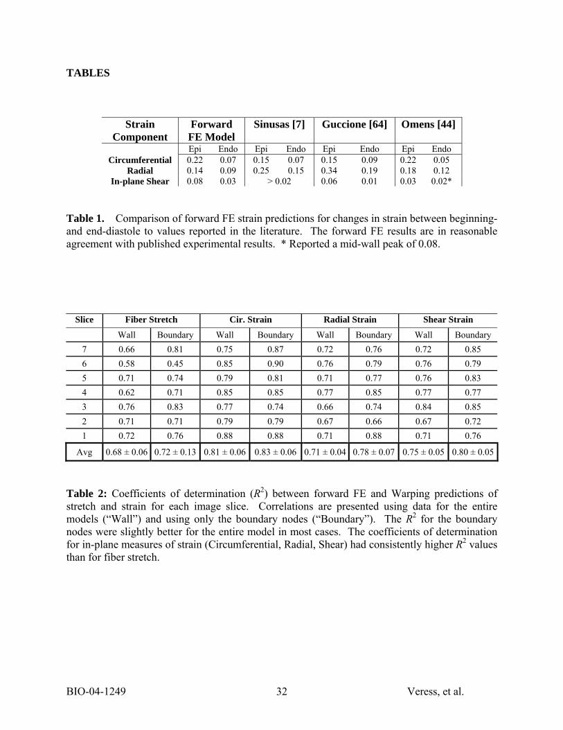
Table 1. Comparison of forward FE strain predictions for changes in strain between beginning- and end-diastole to values reported in the literature. The forward FE results are in reasonable agreement with published experimental results. * Reported a mid-wall peak of 0.08.

Slice Fiber Stretch Cir. Strain Radial Strain Shear Strain

Wall Boundary Wall Boundary Wall Boundary Wall Boundary 7 0.66 0.81 0.75 0.87 0.72 0.76 0.72 0.85 6 0.58 0.45 0.85 0.90 0.76 0.79 0.76 0.79 5 0.71 0.74 0.79 0.81 0.71 0.77 0.76 0.83 4 0.62 0.71 0.85 0.85 0.77 0.85 0.77 0.77 3 0.76 0.83 0.77 0.74 0.66 0.74 0.84 0.85 2 0.71 0.71 0.79 0.79 0.67 0.66 0.67 0.72 1 0.72 0.76 0.88 0.88 0.71 0.88 0.71 0.76

Avg 0.68 ± 0.06 0.72 ± 0.13 0.81 ± 0.06 0.83 ± 0.06 0.71 ± 0.04 0.78 ± 0.07 0.75 ± 0.05 0.80 ± 0.05

Table 2: Coefficients of determination (R2) between forward FE and Warping predictions of stretch and strain for each image slice. Correlations are presented using data for the entire models (“Wall”) and using only the boundary nodes (“Boundary”). The R2 for the boundary nodes were slightly better for the entire model in most cases. The coefficients of determination for in-plane measures of strain (Circumferential, Radial, Shear) had consistently higher R2 values than for fiber stretch.


Fiber Strain Circ. Strain Radial Strain Shear Strain

R2 RMS error

% RMS error R2 RMS

error % RMS

error R2 RMS error

% RMS error R2 RMS

error % RMS

error Baseline Warping 0.67 0.021 29 0.72 0.041 30 0.66 0.025 22 0.70 0.026 36

µ + 24% 0.65 0.021 30 0.69 0.044 32 0.65 0.025 23 0.71 0.026 36

µ - 24% 0.64 0.021 29 0.70 0.042 30 0.65 0.025 23 0.70 0.026 36

C3 + 24% 0.65 0.021 30 0.71 0.040 29 0.66 0.026 23 0.72 0.024 34

C3 - 24% 0.65 0.021 30 0.70 0.041 30 0.66 0.026 23 0.72 0.024 34 Neo-

Hookean 0.57 0.026 39 0.65 0.049 35 0.58 0.032 28 0.69 0.026 37

K*10 0.55 0.021 32 0.63 0.047 42 0.65 0.035 31 0.63 0.028 39

K/10 0.50 0.042 58 0.40 0.079 57 0.30 0.060 53 0.27 0.050 70

Table 3. Effect of changes in material coefficients and constitutive model on coefficients of determination (R2), RMS error (units of strain) and the percent RMS error between the Warping and forward FE predictions for the four measures of strain. “µ + 24%” indicates that results are for the 24% increase in µ the shear modulus.

Fiber Strain Circ. Strain Radial Strain Shear Strain Target Image Data

Set RMS error

% RMS error

RMS error

% RMS error

RMS error

% RMS error

RMS error

% RMS error

early diastolic image 0.017 60 0.034 62 0.025 87 0.023 120 mid-diastolic image 0.016 45 0.028 45 0.024 39 0.020 34 late diastolic image 0.018 34 0.036 54 0.025 35 0.021 31 end-diastolic image 0.021 29 0.041 30 0.025 22 0.026 36

Table 4. The accuracy of the analyses of the intermediate image data sets show similar error magnitudes for RMS error as found in the original validation study. The percent RMS error was found lowest for the end-diastolic study, with the percent RMS error increasing with decreasing average deformation. The percent RMS was the highest in the early diastolic analysis where the RMS error was found to be nearly the magnitude of the measured strain and in the case of the shear measurement the RMS error was larger than the measured shear strain.


FIGURE CAPTIONS

Figure 1: Target (top) and template (bottom) image datasets used in the Warping analysis. The

Target image dataset was created by mapping the template image dataset with displacements

determined from a forward FE simulation of passive diastolic filling.

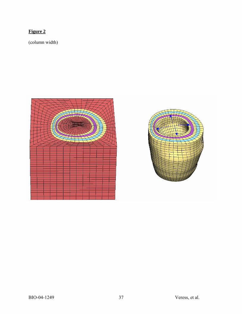
Figure 2: Left - Forward FE model used to create target image. Right – Detail of the LV. Blue

arrows represent the pressure load on the endocardial surface.

Figure 3: Effect of increasing levels of additive noise on the appearance of one slice from the

template image dataset. (A) SNR=0.5, (B) SNR=1, (C) SNR=4, (D) SNR=8, and (E) SNR=16.

Figure 4: Fiber stretch distribution for the forward FE (left) and Warping (right) analyses. The

fiber stretch distributions show good agreement between the FE and the Warping analyses.

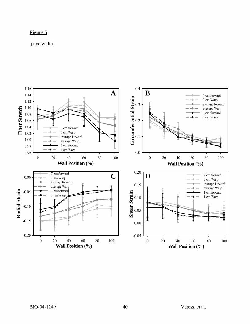
Figure 5: Forward and FE predictions of several measures of local wall deformation at end-

diastole as a function of distance through the myocardial wall (mean ± standard deviation). A –

local fiber stretch. B – circumferential Green-Lagrange strain. C – radial Green-Lagrange

strain. D – in-plane Green-Lagrange shear strain (circumferential/radial). 0% denotes

endocardial surface and 100% denotes epicardial surface. Results are presented for image cross-

sectional slices at 1 cm (light gray), 7 cm (dark gray) and as an average over all slices (black). 7

cm corresponds to the base of the LV and 1 cm is near the apex of the heart. Solid lines indicate

results for the forward FE model and dashed lines indicate results for Hyperelastic Warping.


Error bars show standard deviations. All values are referenced to the undeformed geometry

(beginning-diastole).

Figure 6: Scatter plots of forward FE versus Warping stretch/strains. A - fiber stretch. B -

circumferential strain. C - radial strain. D - in-plane shear strain. Symbols represent different

axial image slices. 7 cm corresponds to the base of the LV and 1 cm is near the apex of the

heart.

Figure 7: Bland-Altman plots of the validation stretch and strain comparison. A - fiber stretch.

B - circumferential strain. C - radial strain. D - in-plane shear strain. The plots show good

agreement between the forward and warping solutions. The central solid line indicates the mean

difference in the data while the heavy dashed lines indicate the boundary of ± 2 standard

deviations.

Figure 8: Effect of signal-to-noise ratio on A - coefficient of determination, and B - the RMS

error (units of strain) for the four measures of deformation.


Figure 1

(page width)


Figure 2

(column width)


Figure 3

(column width)

A B C D E


Figure 4

(column width)

1.16

0.90

Forward Warping


Figure 5

(page width)

Wall Position (%)0 20 40 60 80 100

Shea

r St

rain

-0.05

0.00

0.05

0.10

0.15

0.207 cm forward7 cm Warpaverage forwardaverage Warp1 cm forward1 cm Warp

Wall Position (%)0 20 40 60 80 100

Fibe

r St

retc

h

0.960.981.001.021.041.061.081.101.121.141.16

7 cm forward7 cm Warpaverage forwardaverage Warp1 cm forward1 cm Warp

Wall Position (%)0 20 40 60 80 100

Rad

ial S

trai

n

-0.20

-0.15

-0.10

-0.05

0.007 cm forward7 cm Warpaverage forwardaverage Warp1 cm forward1 cm Warp

Wall Position (%)0 20 40 60 80 100

Cir

cum

fere

ntia

l Str

ain

0.0

0.1

0.2

0.3

0.4

7 cm forward7 cm Warpaverage forwardaverage Warp1 cm forward1 cm Warp

A B

C D


Figure 6

(page width)

Figure 7

(column width)

Forward Shear Strain-0.05 0.00 0.05 0.10 0.15 0.20 0.25

War

ping

She

ar S

trai

n

-0.05

0.00

0.05

0.10

0.15

0.20

0.25

7 cm6 cm5 cm 4 cm3 cm2 cm1 cm

R2 = 0.70Slope = 0.91y-int = 0.008

Forward Radial Strain -0.25-0.20-0.15-0.10-0.050.000.05

War

ping

Rad

ial S

trai

n

-0.25

-0.20

-0.15

-0.10

-0.05

0.00

0.05


R2 = 0.75Slope = 0.95y-int = -0.01

Forward Fiber Stretch 0.95 1.00 1.05 1.10 1.15 1.20

War

ping

Fib

er S

tret

ch

0.95

1.00

1.05

1.10

1.15

1.20

7 cm6 cm5 cm4 cm3 cm2 cm 1 cm

R2 = 0.67Slope = 1.00y-int = -0.002

Forward Circumferential Strain-0.1 0.0 0.1 0.2 0.3 0.4 0.5W

arpi

ng C

ircu

mfe

rent

ial S

trai

n

-0.1

0.0

0.1

0.2

0.3

0.4

0.5


R2 = 0.76Slope = 0.97y-int = 0.02

A B

C D


Figure 7

(page width)

-0.1

-0.05

0

0.05

0.1

1 1.05 1.1 1.15

Stretch (λ )

Diff

eren

ce in

Str

etch

DifferenceMean DifferenceMean Diff. ± 2SD

-0.15-0.1

-0.050

0.050.1

0.15

-0.25 -0.2 -0.15 -0.1 -0.05 0

Radial Strain

Diff

eren

ce in

Str

ain

-0.15-0.1

-0.050

0.050.1

0.15

0 0.1 0.2 0.3 0.4

Shear Strain

Diff

eren

ce in

Str

ain

-0.15-0.1

-0.050

0.050.1

0.15

0 0.1 0.2 0.3 0.4

Circumferential Strain

Diff

ernc

e in

Str

ain

A B

C D


Figure 8

(column width)

S ig n a l-to -N o ise R a tioIn f 1 6 .0 8 .0 4 .0 2 .0 1 .0 0 .5

RM

S Er

ror

0 .0 1

0 .0 2

0 .0 3

0 .0 4

0 .0 5

0 .0 6

0 .0 7

0 .0 8S ig n a l-to -N o ise R a tio

In f 1 6 .0 8 .0 4 .0 2 .0 1 .0 0 .5

R2 Val

ue

0 .1

0 .2

0 .3

0 .4

0 .5

0 .6

0 .7

0 .8

S tre tc hC irc u m fe re n tia l S tra inR a d ia l S tra inS h e a r S tra in

A

B

Documents

Measurement of Strain in the Left Ventricle during ... · PDF fileMeasurement of Strain in the Left Ventricle during Diastole with cine ... linear and undergoes finite deformation